Accelerating Genetic Programming using GPUs

Abstract

Genetic Programming (GP), an evolutionary learning technique, has multiple applications in machine learning such as curve fitting, data modelling, feature selection, classification etc. GP has several inherent parallel steps, making it an ideal candidate for GPU based parallelization. This paper describes a GPU accelerated stack-based variant of the generational GP algorithm which can be used for symbolic regression and binary classification. The selection and evaluation steps of the generational GP algorithm are parallelized using CUDA. We introduce representing candidate solution expressions as prefix lists, which enables evaluation using a fixed-length stack in GPU memory. CUDA based matrix vector operations are also used for computation of the fitness of population programs. We evaluate our algorithm on synthetic datasets for the Pagie Polynomial (ranging in size from $4096$ to $16$ million points), profiling training times of our algorithm with other standard symbolic regression libraries viz. gplearn, TensorGP, KarooGP. In addition, using $6$ large-scale regression and classification datasets usually used for comparing gradient boosting algorithms, we run performance benchmarks on our algorithm and gplearn, profiling the training time, test accuracy, and loss. On an NVIDIA DGX-A100 GPU, our algorithm outperforms all the previously listed frameworks, and in particular, achieves average speedups of $119\times$ and $40\times$ against gplearn on the synthetic and large scale datasets respectively.

I Introduction

In recent years, there has been a widespread increase in the use of GPUs in the field of machine learning and deep learning, because of their ability to massively speedup the training of models. This is mainly due to the large parallel processing ability of GPUs, which can process multiple inputs using Single Instruction Multiple Data (SIMD) intrinsics. Genetic Programming (GP) belongs to a class of machine learning algorithms with several inherent parallel steps. As such, it is an ideal domain for GPU based parallelization.

GP as a technique involves the evolution of a set of programs based on the principles of genetics and natural selection. It is a generalized heuristic search technique, which searches for the best program optimizing a given fitness function. Because of it’s generalizability, the technique finds applications ranging from machine learning to code synthesis [1].

However, in practice, it is difficult to scale GP algorithms. Fitness evaluation of candidate programs in GP algorithms is a well-known bottleneck, and there are multiple previous attempts to overcome this problem - either through parallelization of the evaluation step , or by eliminating the need for fitness computations itself through careful initialization and controlled evolution [2].

In this paper, we introduce a parallelized version of the generational GP algorithm to solve symbolic regression problems. We use a stack-based GP model for program evaluation (inspired by [3]). Our algorithm can also be used to train binary classifiers, where the classifier output corresponds to the estimated equation of the decision boundary.

We evaluate our accelerated algorithm by providing execution time benchmarks for program evaluation. The same benchmarks are also run on other standard libraries like gplearn [4] and TensorGP [5], for comparing training speeds. We also study the effect of population size and dataset size on the final time taken for training. The benchmarks are run using synthetic datasets for the Pagie Polynomial [6] as well as $6$ large-scale regression and classification datasets usually used for the comparison of gradient boosting frameworks [7].

Our work has been implemented as an algorithm in cuML [8], a GPU accelerated machine learning library with an API inspired by the scikit-learn library [9].

The rest of this paper is organized as follows. Section II gives an overview of existing literature, and introduces the generational GP algorithm. It also discusses other existing GP frameworks and libraries. Section III presents our parallel algorithm to perform symbolic regression using genetic programming, along with some implementation details and challenges faced. Section IV describes our experimental setup and presents our benchmarking results. Finally Section V concludes the paper and outlines directions for further optimizations and future research.

II Background and Related Work

In this section, we describe in detail the generational GP algorithm [10, 11], which serves as a base for all of our parallelization experiments. Later on, we also give a brief description of some existing GP libraries.

Since the domain of our problem is symbolic regression, we note that the program for our GP system is a mathematical expression, represented as an expression tree. Each program comprises a list of functions (of varying arity) and terminals, where terminals collectively denote both variables and constants.

II-A The Generational GP Algorithm

The generational GP algorithm gives us a method to evolve candidate programs using the principles of natural selection. There are $3$ main steps involved in the algorithm.

1. Selection — In this step, we decide on a set of programs to evolve into the next generation, using a selection criterion.

2. Mutation — Before promoting the programs selected in the previous step to the next generation, we perform some genetic operations on them.

3. Evaluation — We again evaluate the mutated programs on the input dataset to recompute fitness scores.

The above $3$ steps are formalized in Algorithm 1.

Algorithm 1 The Generational GP Algorithm

1:procedure GP-FIT($dataset$)

2:     $curr\leftarrow$Initialize population

3:     Evaluate($curr,dataset$)

4:     repeat

5:         $next\leftarrow$ Select($curr$)

6:         $next\leftarrow$ Mutate($next$)

7:         Evaluate($next,dataset$)

8:         $curr\leftarrow next$

9:     until user defined termination criteria on $curr$ not met

10:     return $curr$$\triangleright$ The final generation of programs

11:end procedure

Koza [1] lists $3$ standard initialization techniques for GP programs. They are as follows.

• Full initialization — All trees in the current generation are dense, that is, all the terminals(variables or constants), are at a distance of max_depth from the root.

• Grow initialization — All trees grown in the current generation need not be dense, and some nodes that have not reached max_depth can also be terminals.

• Ramped half-and-half — Half of the population trees are initialized using the Full method, and the other half is initialized using the Grow method. (the common usage)

II-A1 Selection

Selection is the step where individual candidates from a given population are chosen for evolution into the next generation. According to Goldberg and Deb [12], the commonly used selection schemes in GP are as follows:

• Tournament selection — Winning programs are determined by selecting the best programs from a subset of the whole population(a tournament). Multiple tournaments are held until we have enough programs selected for the next generation.

• Proportionate selection — Probability of candidate program being selected for evolution is directly proportional to its fitness value in the previous generation

• Ranking selection — The population is first ranked according to fitness values, and then a proportionate selection is performed according to the imputed ranks.

• Genitor(or steady state) selection — The programs with high fitness are carried forward into the next generation. However, the programs with low fitness are replaced with mutated versions of the ones with higher fitness.

In the implementation of our algorithm, only parallel tournament selections are supported through the use of a CUDA kernel. This is in an effort to make our implementation consistent with gplearn [4], which also only implements tournament selection.

II-A2 Mutation

As discussed earlier, the winning programs after selection are not directly carried forward into the next generation. Rather, mutations or genetic operations are applied on the selected programs, in order to produce new offspring. Stephens [4] lists some commonly used mutation operations, which are as follows.

• Reproduction

• Point mutations

• Hoist mutations

• Subtree mutations

• Crossover mutations

In our code we provide support for all the above listed genetic operations, along with a modified version of the crossover operation to account for tree depth.

In Reproduction, as the name suggests, the current winning program is simply cloned into the next generation of programs.

In Point mutations, we modify randomly chosen nodes of a given parent program in place. In the context of symbolic regression, we replace terminals(variables or constants) with terminals, and functions with another functions of the same arity. This mutation has the effect of reintroducing extinct functions and variables into the population, helping maintain diversity.

In Hoist mutation, a random subtree from the winner of the tournament is taken. Another random subtree is selected from this subtree as a replacement for the first subtree from the program. This mutation serves to reduce bloating of programs(with respect to depth) with increase in number of generations.

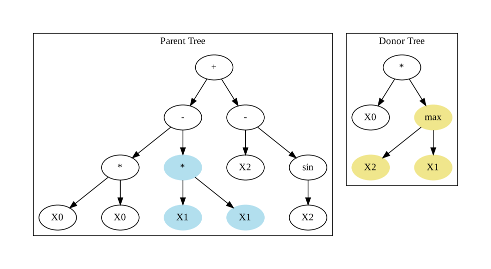
(a) The parent and donor expression trees, both selected through tournaments are shown here.

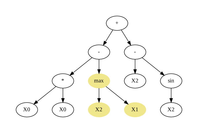
(b) The child expression tree after replacing a subtree of the parent with that of the donor.

Figure 1: Visualizing crossover mutations for a given parent and donor expression tree.

In Subtree mutation, we perform a crossover operation between the parent tree and a randomly generated program. Similar to point mutations, this also serves as a method to increase new terminals and extinct functions in the next generation of programs.

In Crossover mutation, the genetic information in $2$ programs of a given population are mixed. We first determine a parent and a donor program using $2$ separate tournaments. A random subtree of the parent program is then replaced with a subtree from the donor program. We show a sample visualization of the crossover operation in Figure 1.

Figure 1 can again be used to visualize subtree mutations. The only difference between crossover and subtree mutations is that in subtree mutations, the donor program in Figure 1(a) is now a randomly generated tree.

II-A3 Evaluation

Once the population for the next generation is decided after selection and mutation, the fitness of all programs in the new generation is recomputed. This step is the major bottleneck when scaling the generational GP algorithm to bigger datasets and bigger populations, as the evaluation is independent for every program and every row of the input dataset.

II-B Existing Libraries and Their Coverage

Table I (mostly reproduced from [13]) lists some common libraries used for genetic programming.

TABLE I: Some existing GP frameworks along with language and device support

Framework	Language	Compute Type
KarooGP	Python	CPU/GPU
TensorGP	Python	CPU/GPU
DEAP	Python	CPU
gplearn	Python	CPU
ECJ	Java	CPU

Among the libraries listed in Table I, both TensorG P[5] and KarooGP [14] use the TensorFlow python framework to perform fitness evaluation the GPU. However, while KarooGP uses TensorFlow’s graph execution model, where the computation graph is compiled into an optimized DAG, TensorGP uses TensorFlow’s eager execution model, where expressions are evaluated immediately without the overhead of graph construction. The GPU parallelization here is through the use of TensorFlow-based vectorization, and not the explicit use of CUDA.

DEAP [15] is another commonly used Evolutionary Computing framework in Python implements a parallelized version of the GP framework. However, it offers only CPU based parallelization.

Gplearn [4] is another Python framework which provides a method to build GP models for symbolic regression, classification and transformation using an API which is compatible with scikit-learn [9]. It also provides support for running the evolutionary process in parallel. The base code that is parallelized on GPUs in this paper is largely inspired by gplearn.

The ECJ Evolutionary Computing Toolkit [16] is a Java library for many popular EC algorithms, with an emphasis towards genetic programming. Almost all aspects of Algorithm 1 are governed by a hierarchy of user-provided parameter files and classes, and the framework itself is designed for large, heavyweight experimental needs. Using ECJ parameter files, it is also possible to define custom GP pipelines with user-defined evolution strategies.

III CUDA Accelerated Genetic Programming

This section presents the implementation details of our parallel algorithm to perform genetic programming using CUDA. We first talk about a way to represent programs on the GPU. This is then followed by a description of the device side data structures used. We then give an overview of our modified GP algorithm, describing GPU-side optimizations for the selection, and evaluation step in detail. We also include details about the fitness computation step which comes after the evaluation step. Finally, we talk about the various challenges faced during the implementation of the modified algorithm, and the workarounds to avoid these problems.

In this implementation, we use a fixed list of functions with a maximum arity of $2$. We assume that the input dataset and actual output provided for training already resides in GPU memory, and are stored in a column-major order format.

III-A Program Representation

We define a struct for a program containing the following components.

• An array of operators and operands of the underlying expression tree stored in Polish (prefix) notation.

• A length parameter corresponding to the total number of nodes in the expression tree.

• A raw fitness parameter containing the score of the current tree on the input data-set.

• The depth of the current expression tree.

LABEL:lst:programstruct shows the internal definition of the program struct used in our code. nodes is the prefix list used to store the nodes of the underlying expression tree. The content of nodes is decided through the mutation step. Evaluation and fitness computations are used for the computation of the raw_fitness_ field.

⬇

1struct program {

2 node *nodes; // underlying AST nodes

3 int len;

4 int depth;

5 float raw_fitness_; // fitness on input dataset

6 metric_t metric; // loss function type

7};

Listing 1: A simplified version of our code for the program struct, representing a single expression tree. This entire structure is copied over and evaluated on the GPU.

The entire population for a given generation is thus stored in an Array of Structures (AoS) format. The evaluation using a stack is almost similar to the way the Push3 system [17] evaluates GP programs, with the sole exception being the reverse iteration due to the prefix notation chosen for the trees.

Prefix notation was used for the representation of nodes to aid with the process of generating random programs, where we directly generate a valid prefix-list on the CPU.

III-B Device Side Data Structures

In order to perform tournament selection and evaluation on the GPU, we use the following device side data-structures.

• Philox Random Number Generator (RNG) — We use the Philox counter-based RNG [18] implemented in raft [8] to generate random global indices for tournament selection inside the selection kernel.

• Fixed size device stack — We define a fixed size stack using a custom class, implementing the push, pop methods as inline __host__ __device__ functions. To avoid global memory accesses and encourage register look-ups for internal stack slots, the push and pop operations are implemented using an unrolled loop over all the available slots.

Our kernels for both selection and program execution have been written in a way to eliminate any need for synchronization or barriers.

III-C The Parallel GP Algorithm

In this section, we again outline the individual steps of the generational GP Algorithm described in Section II-A. However, each step contains details specific to our implementation. For our implementation, the selection and evaluation steps are performed on the GPU, whereas mutations are carried out on the CPU.

Before performing any of the standard steps, we decide on the type of mutation through which the next generation program is produced. This mutation type selection is governed by user defined probabilities for the various types of mutations. This step is important, as we need to determine the exact number of selection tournaments to be run (as crossover mutations require $2$ tournaments to decide the parent and donor trees).

Once the required number of tournaments has been decided, we move on to the selection step.

III-C1 Selection

Tournament Selections are carried out in parallel using a CUDA kernel. For a given tournament size $k$, after computing the required number of tournaments, a kernel is launched, where each thread corresponds to a unique tournament. Each thread performs the following set of computations.

• Generate $k$ random program indices using a Philox RNG.

• Find the optimal index value among the $k$ indices with respect to fitness values (after accounting for both the criterion and the parsimony coefficient penalty).

• Record the optimal index computed in the previous step as the current thread’s winner.

Depending on the type of the loss function, the criterion can either favour smaller or larger fitness function values. The parsimony coefficient is another constant parameter used to control bloating of programs, by adding a penalty proportional to the length of candidate programs. For a given program $p$ with parsimony coefficient $c$ and a criterion favouring smaller fitness values, Equations 1 and 2 compute the adjusted fitness values used for computing optimal indices.

$$p.penalty =c~{}(p.len)$$ (1)

$$p.fitness =p.raw\_fitness+p.penalty$$ (2)

III-C2 Mutation

The mutation of programs takes place on the CPU itself. Since every program has its own specific mutation, a GPU based implementation would lead to significant warp divergence, especially when identifying sub-trees in a program (since a different length sub-tree would be selected for each program during crossover, subtree or hoist mutations).

We implement all the mutations mentioned in section II-A with a slight modification to the crossover operation in order to constrain the depth of the output tree. We call this modification a hoisted crossover. In a hoisted crossover operation, we initially perform a crossover between the parent tree and the donor tree. The selected subtree of the donor is then repeatedly hoisted onto the parent tree until the depth of the resultant tree is less than the maximum evaluation stack size.

This modification is necessary for our code since a stack of fixed size $m$ can only evaluate a tree of depth $m-1$ (assuming the maximum function arity is $2$).

At the end of mutations, we allocate and transfer the newly created programs onto GPU memory, in order to evaluate them on the input data-set. In order to save on device memory, we also deallocate the GPU memory of the previous population trees. Some of the challenges we faced due to the nested nature of program representation during the cudaMemcpy operations between host and device memory are listed in Section III-D.

III-C3 Evaluation

We divide the evaluation portion into $2$ steps, an execution step and a fitness metric computation step.

In the execution step, all programs in the new population are evaluated on the given data-set, to produce set of predicted values. If $n$ is the population size, and $m$ is the number of samples in the input dataset, then we launch an execution kernel with a 2D grid of dimension $(\left\lceil m/256\right\rceil,n)$ with $256$ threads per block. Each thread has its own device side stack which evaluates a prefix list based program on a specific row.

We note here that to avoid thread divergence in the execution kernel, it is important to ensure that each thread block executes on different rows of the same program. More details about this can be found in Section III-D.

In the fitness metric computation step, for every program, we compute fitness using a user-selected loss function. The inputs to the loss function are the program’s output values (from the execution step) and the actual outputs.

Since the fitness computation is the same for all programs, we computed loss for all programs in parallel on the GPU. The computation was structured as a $2$ step operation as follows.

• A matrix vector operation was used to compute row-wise loss for the input dataset, with the columns of the predicted value matrix corresponding to population programs. The actual output vector is broadcasted along all columns of the predicted value matrix in this step.

• For every column of the loss matrix computed in the previous step, a weighted sum reduction operation is carried out to get a vector containing final raw fitness values for all programs.

Both of the above steps were implemented using the linear algebra and statistics primitives present in the raft library [8]. In our implementation, weighted versions of the following $6$ standard loss functions were implemented:

• Mean Absolute Error (MAE)

• Mean Square Error (MSE)

• Root Mean Square Error (RMSE)

• Logistic Loss (binary loss only)

• Karl Pearson’s Correlation Coefficient

• Spearman’s Rank Correlation Coefficient

During the implementation of Spearman’s Rank Correlation, we used the thrust library from Nvidia to generate ranks for the given values. The Karl Pearson’s coefficient is then computed for the imputed ranks.

The default fitness function is set as MAE, in an effort to be consistent with gplearn [4].

III-D Challenges Faced

In this section, we briefly talk about some challenges faced during the implementation of our parallel GP algorithm.

III-D1 Thread divergence and Global Memory Access

In the evaluation step, during function computations in the execution phase, we check for equality of the current function with $33$ pre-defined functions, using if-else conditions on the node type.

Since CUDA executes statements using warps of $32$ threads in parallel, when it encounters an if-else block inside a kernel which is triggered only for a subset of the warp, both the if and else blocks are executed by all threads. During the execution of the if block, the threads which do not trigger the if condition are masked, but still consume resources, with the same behaviour exhibited for the else block. This increases the total execution time as both blocks are effectively processed by all warp threads.

To avoid this behaviour in our code, we ensure that within every thread-block of the execution kernel, all threads execute the same program. This ensures that all threads in a warp will always take the same branch during node identification, and thus avoid divergence during a single stack evaluation.

In the implementation of push and pop operations for the device side stack, we avoid trying a possible dereference using global memory index(the current number of elements in the stack) by using an unrolled loop for stack memory access. This is again safe from thread divergence because we ensure that within a thread-block, all threads evaluate the same program.

III-D2 Memory Transfers and Allocation

Since used an AoS representation for the list of programs and each program has a nested pointer for the list of nodes in it, we are forced to perform at least $2$ cudaMemcpy operations per program in a loop spanning the population size. One of the copy operations is for the list of program nodes, and the other copy is to capture the metadata about the nodes, and the other copy is for the program struct itself.

Since all our computations are ordered on a single CUDA stream, transferring programs back and forth the device in a loop slows down the overall time for training. However, in our experiments, we observed that the dominant contributor to execution time was the evaluation step, and not memory transfers.

IV Experimental Evaluation

In this section, we will describe the various experiments ran to evaluate the performance of our algorithm’s implementation(henceforth referred to as cuml) against the other GP libraries mentioned in Section II-B. In particular, we consider the gplearn [4], KarooGP [14] (only GPU), and TensorGP [5] (both CPU and GPU) libraries in our benchmarks.

We run $2$ sets of benchmarks on both synthetic and large-scale datasets. For the synthetic dataset benchmarks, we follow the framework laid out in [13] to compare evaluation times for all the above GP libraries on seven 2D regression datasets ranging in size from $4096$ to $16$ million points for an average over $10$ runs.

For the large-scale benchmarks, we consider $6$ real world datasets commonly used for the comparison of gradient boosting frameworks. We perform a detailed comparison of the performance of both gplearn and cuml on these datasets, profiling training time for an average over $3$ runs. Since gplearn was our reference for implementation, we used it for comparison with cuml on large-scale benchmarks. In addition, we also compare the test accuracy and loss for both libraries initialized with the same hyper-parameters.

Before exploring the benchmarks on the synthetic datasets, we note that field of GP, especially for symbolic regression suffers from a lack of standardized benchmarks. This problem is explored by a few studies [19], which attempt to quantify and list candidate GP problems. In our experiments, we follow the guidelines laid out in these studies.

All experiments were carried out in a compute cluster with the specifications listed in Table II.

TABLE II: Hardware and software setup for carrying out all experiments

Component	Specification
CPU model	Intel(R) Xeon(R) Silver 4110 @ 2.10GHz
GPU model	NVIDIA DGX-A100
CTK Version	11.2
# CPU cores	16
RAM	64 GB
OS	Ubuntu 20.04 LTS Server

IV-A Synthetic Benchmarks

Our synthetic benchmarks were motivated by [13], and follow a similar flow for testing execution times between different libraries. We also compare the variation of best fitness values for cuml with increasing dataset size.

IV-A1 Setup

In all symbolic regression runs, we try to approximate the Pagie Polynomial [6] over the domain $(x,y)\in[-5,5]^{2}$.

$$f(x,y)=\frac{1}{1+x^{-4}}+\frac{1}{1+y^{-4}}$$ (3)

We generate $7$ synthetic datasets by uniformly subsampling points from the domain $(x,y)\in[-5,5]\times[-5,5]$. The initial dataset is generated by subsampling a random square grid of dimensions $64\times 64=4096$ points from the domain. To generate the remaining datasets, the length of the grid is iteratively doubled until we subsample a grid of side $4096$ containing over $16$ million points.

TABLE III: Common parameters used for the synthetic dataset benchmarks

Parameter	Value
Runs	10
Number of Generations	50
Population size	50
Generation Method	Ramped Half and Half
Fitness Metric	RMSE
Crossover probability	0.7
Mutation probability	0.25
Reproduction probability	0.05
Function Set	$\{+,-,*,\div,\sin,\cos,\tan\}$

Table III lists some common parameters used for training GP models for all libraries. The Ramped Half and Half method was used for tree initialization in all libraries. Root Mean Square Error (RMSE) on the training dataset was chosen as the fitness metric for all population trees.

IV-A2 Experimental Results

A total of $320$ runs were performed across the $5$ different GP libraries to produce the results in this section. We compare the average execution time for $10$ runs for all synthetic datasets, followed by an analysis of the evolution of fitness for cuml.

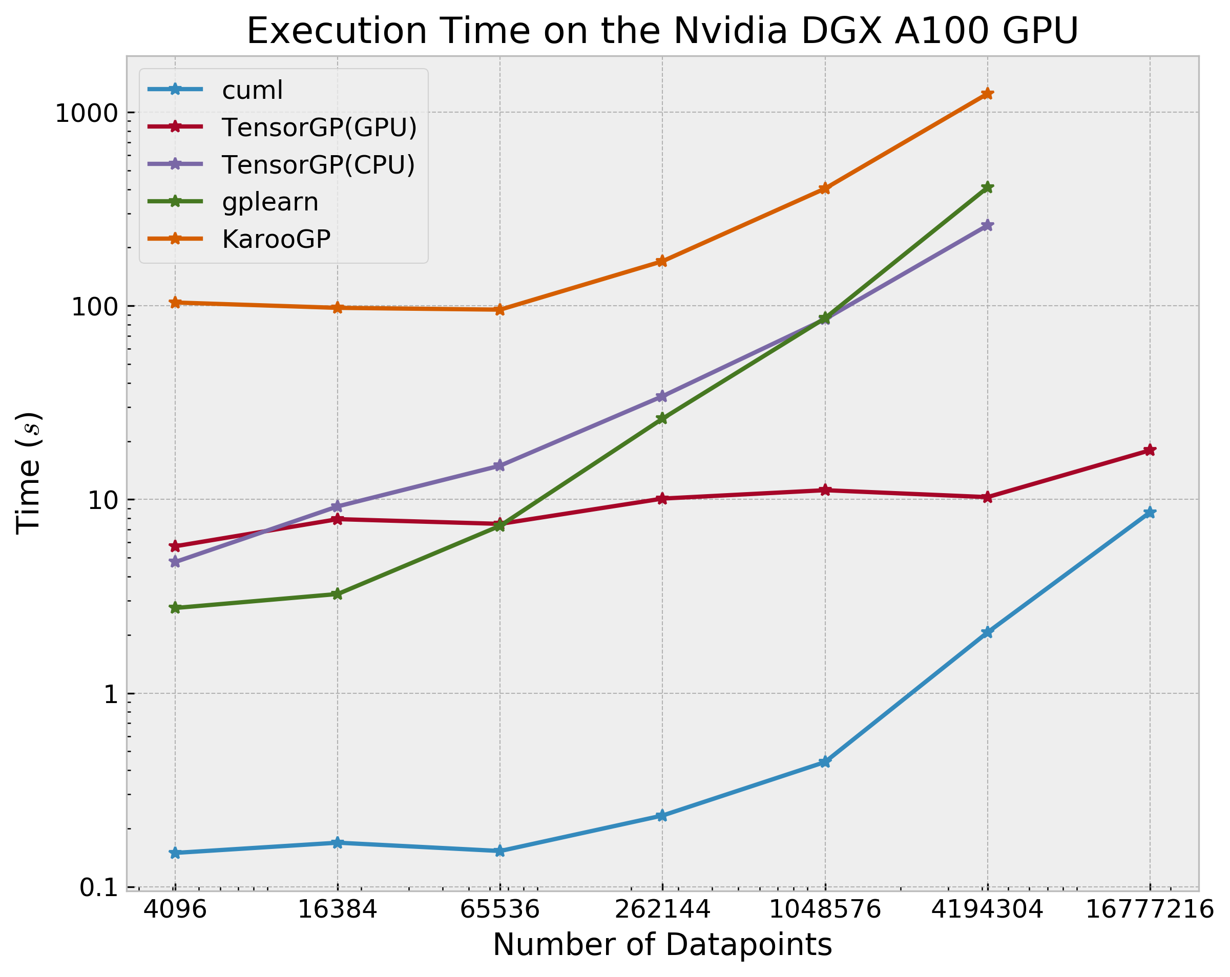
Figure 2: Log-Log Plot of Execution Time for various libraries (lower is better). The number of rows considered exponentially increases from $4096$ to over $16$ million.

Figure 2 showcases the variation of execution time with increasing dataset size for different datasets, averaged over $10$ runs on each dataset. The same average values are also recorded in Table IV.

TABLE IV: Table containing mean execution time (lower is better) for a GP run (averaged across $10$ runs) in seconds for different libraries. DNF denotes that the test did not finish within $2$ hours.

# Rows 4096 16384 65536 262144 1048576 4194304 16777216 cuml 0.150 0.169 0.153 0.233 0.441 2.057 8.579 TensorGP (GPU) 5.736 7.916 7.482 10.109 11.168 10.284 17.941 TensorGP (CPU) 4.757 9.215 14.953 34.158 85.380 260.114 DNF gplearn 2.753 3.250 7.320 26.167 86.369 408.217 DNF KarooGP 104.050 97.639 95.586 170.060 403.359 1245.424 DNF

From Table IV, we note that cuml takes $3$ seconds to train the $4$ million row dataset, whereas gplearn takes around $408$ seconds on the same input. When taking a mean average of runtime across all datasets and runs, we achieve an average speedup of $119\times$ in training time with respect to gplearn, with a maximum speedup of $135\times$ in the $4$ million row dataset.

Since KarooGP uses the TensorFlow graph execution model, it is possible that more time is spent in building and modifying the session graph in every generation compared to fitness evaluation.

From the graph in Figure 2, as well as Table IV, we see that the TensorGP (GPU) approach consistently outperforms gplearn, KarooGP and TensorGP (CPU) on datasets with more than $65536$ points. Since TensorGP (GPU) uses TensorFlow’s GPU backend with eager execution, time is not spent in building an optimized computation DAG for every program. This in turn increases the speed of parallel evaluation.

When comparing cuml to the rest of the libraries in Figure 2 and Table IV, we note that cuml is the fastest among all libraries on all inputs. cuml also outperforms TensorGP(GPU), since the algorithm batches the computation of fitness across the entire population and dataset.

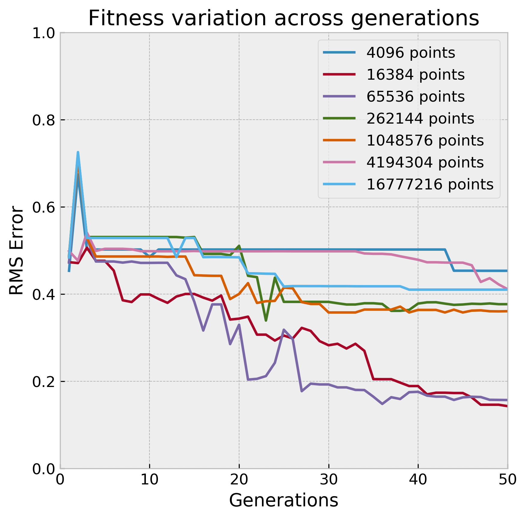
Figure 3: Variation of RMS error of with the number of generations for cuml on the synthetic datasets. The error value corresponds to the fitness value of the best tree in every generation.

For cuml, Figure 3 showcases the variation of the fitness score of the best tree in every generation for all datasets. It is easy to notice that the $1$ million row test set displays a consistently decreasing error with increasing number of generations. However, we notice that the overall fitness value does not decrease even with an increase in the total number of evaluation data points in the same domain.

Hence, we can conclude that bigger and more granular datasets do not help if we are performing symbolic regression to find the Pagie Polynomial, a result in line with [13].

IV-B Large-Scale Benchmarks

We run benchmarks on $6$ large datasets usually used for the comparison of gradient boosting frameworks. In particular, we consider the Airline [20], Credit card fraud [21], Higgs [7], and Epsilon [22] datasets for symbolic classification, and the Airline Regression [20] and YearPredictionMSD datasets [7] for symbolic regression.

IV-B1 Setup

Table V lists all the details of the datasets used in this benchmark. All the classification problems listed are binary classification problems. The train-test split for every dataset is done according to the descriptions provided for every dataset source.

We run this benchmark only on the cuml and gplearn library. Since cuml is a GPU accelerated re-implementation of gplearn, our aim is to achieve similar average test scores for both the libraries along with a decrease in training time.

TABLE V: All large-scale datasets considered for benchmarks.

Name Rows Columns Task Airline 115M 13 Classification Airline Regression 115M 13 Regression Fraud 285K 28 Classification Higgs 11M 28 Classification Year 515K 90 Regression Epsilon 500K 2000 Classification

To speed up the execution times for gplearn, every GP run was parallelized using $8$ jobs(using the Python joblib library).

Table VI lists all common parameters used for training GP models for both cuml and gplearn. RMS Error is again used as the fitness metric for all regression datasets, while Logistic loss is used as the fitness metric for all the binary classification datasets.

TABLE VI: Common parameters used for the large dataset benchmarks.

Parameter	Value
Runs	3
Number of Generations	50
Population size	35
Tournament size	4
Generation Method	Ramped Half and Half
Fitness Metric	RMSE / Logistic Loss
Crossover probability	0.7
Subtree mutation probability	0.1
Point mutation probability	0.1
Hoist mutation probability	0.05
Reproduction probability	0.05
Parsimony coefficient	0.01
Function Set	$\{+,-,*,\div,\sin,\cos,\tan\}$

IV-B2 Experimental Results

A total $36$ GP runs were performed on the cuml and gplearn to produce the results in this section. We compare the average training time taken by both libraries, followed by a comparison of results on the test dataset for both libraries.

Figure 4 showcases the variation of execution time for both cuml and gplearn for all the datasets listed in Table V. The same values can be found in Table VII.

From Table VII we find that cuml achieves a mean speedup of $40\times$ in training with respect to gplearn across all the datasets, with a maximum speedup of $713\times$ in the Epsilon dataset. The tremendous speedup observed in the Epsilon dataset (which has $2000$ columns) can be attributed to the coalesced memory access resulting from the column-major order storage of the input data in GPU memory. On the Airline and Airline regression datasets, $2$ datasets with more than $100$ million rows, cuml achieves an average speedup of $42\times$ and $32\times$ with respect to gplearn(parallelized using $8$ jobs) in training time.

TABLE VII: Table containing mean execution time (lower is better) for a GP run (averaged across $3$ runs) in seconds for both cuml and gplearn.

Dataset cuml gplearn Airline 50.088 2122.619 Airline Regression 55.935 1810.712 Epsilon 0.170 121.543 Fraud 0.264 19.448 Higgs 2.250 272.140 Year 0.248 26.444

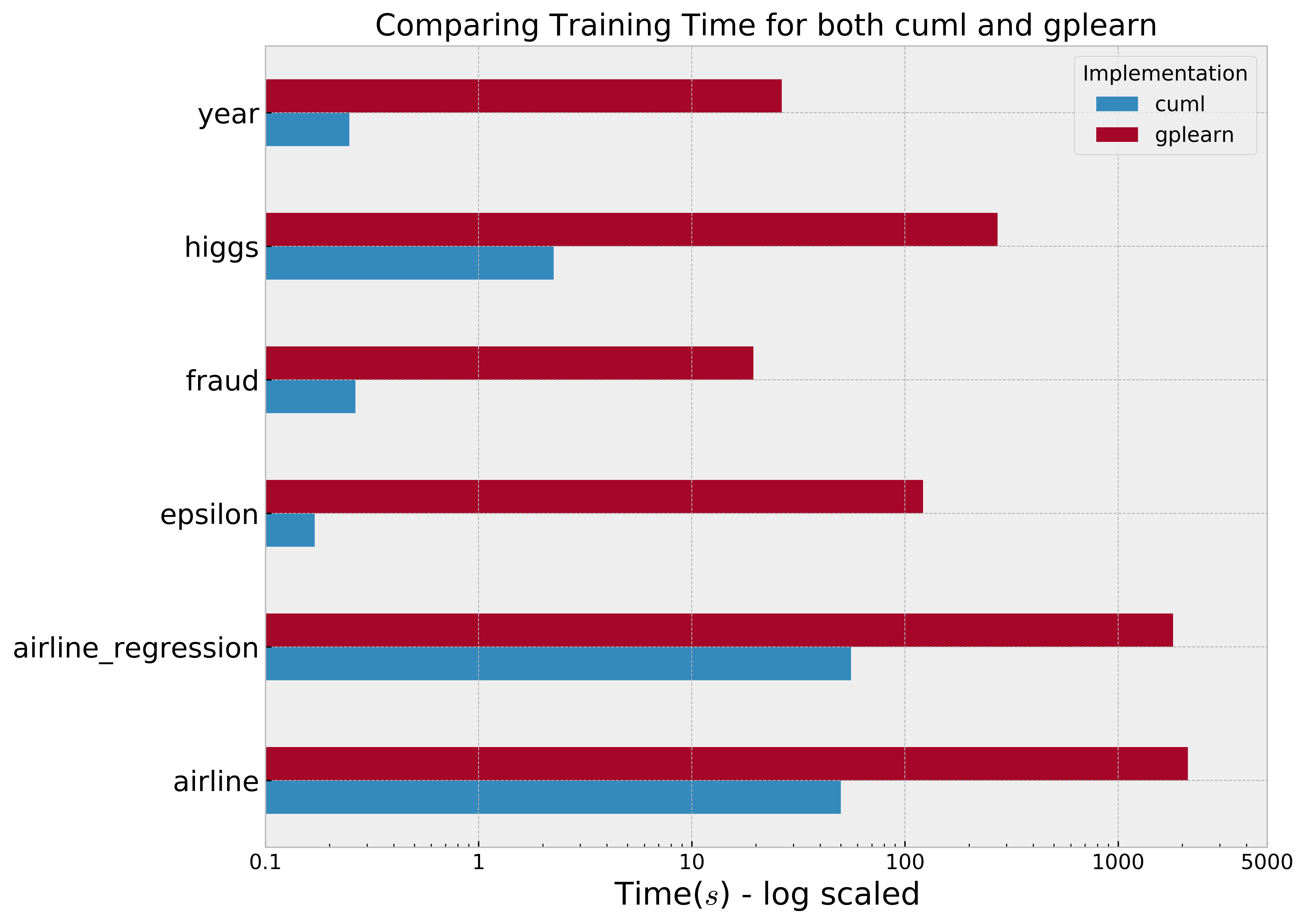
Figure 4: Bar graph showcasing the difference in training time for both cuml and gplearn (lower is better). A speedup in training time is observed for all datasets when using cuml.

Table VIII compares the symbolic classification accuracy on the test split of all classification datasets for both cuml and gplearn on the best program at the end of the GP run. We note that for all the datasets, the test accuracy for both the libraries lie with $5\%$ of each other, with cuml outperforming gplearn in the Higgs and Epsilon datasets.

TABLE VIII: Table containing classification accuracy values (normalized to $[0,1]$) on the test split of all datasets for both cuml and gplearn (higher is better).

Classification cuml gplearn Datasets Airline 0.474572 0.525428 Epsilon 0.560250 0.520487 Fraud 0.998280 0.998280 Higgs 0.567743 0.530103

Table IX compares the test RMS Error obtained at the end of the GP run for both gplearn and cuml. We again notice that the error values obtained for both libraries are almost the same, especially in the case of the Airline Regression dataset. For the Year prediction dataset, we see that cuml slightly outperforms the gplearn with respect to the test RMS error.

TABLE IX: Table containing RMS Error values on the test split of all datasets for both cuml and gplearn (lower is better).

Regression cuml gplearn Datasets Airline Regression 31.024 30.900 Year 825.138 840.209

We note that Tables VIII and IX do not allow to draw a conclusion on which library produces better results for symbolic regression in general. This is because the final fitness values achieved are highly sensitive to the initialization of programs, which is randomized. Rather, the only goal of the test metrics is to help us verify similar behaviour of fitness values across libraries on the same datasets, when initialized with the same training hyperparameters.

V SUMMARY AND FUTURE WORK

In this paper, we accelerated genetic programming based symbolic regression and classification on the GPU. We do this by parallelizing the selection and evaluation step of the generational GP algorithm. We introduce a prefix-list representation for expression trees, which are then evaluated using an optimized stack on the GPU. Fully vectorized routines for standard loss functions are also provided, which can be used as fitness functions during the training of a genetic population of programs. At the end of a run, our algorithm returns the entire set of evolved programs for all generations. The most optimal program from the last generation of programs can be used as a potential symbolic regressor or classifier.

Our experimental results using both synthetic and large scale datasets indicate that our implementation of genetic programming is significantly faster when compared to existing CPU and GPU parallelized frameworks. Performance benchmarks indicate that our implementation achieves an average speedup $119\times$ and $40\times$ against gplearn, a CPU parallelized GP library on the synthetic and large scale datasets respectively.

In the future, we are planning to add support for custom function sets and loss functions during GP runs. We are also planning to address the problem of multiple memory transfers between the CPU and the GPU by slightly modifying the underlying program representation without compromising on the stack based evaluation model for programs. In addition, we are also planning to implement a Python layer over the current CUDA/C++ based implementation of the algorithm.

This paper and the research behind this would not have been possible without the generous support of the NVIDIA AI Technology Center (NVAITC), which facilitated this collaborative work between NVIDIA and IIT Madras.

References

- [1] J. R. Koza, Genetic Programming: On the Programming of Computers by Means of Natural Selection. Cambridge, MA, USA: MIT Press, 1992.
- [2] J. A. Biles, “Autonomous genjam: eliminating the fitness bottleneck by eliminating fitness,” in Proceedings of the GECCO-2001 workshop on non-routine design with evolutionary systems, vol. 7. Morgan Kaufmann San Francisco, CA,, USA, 2001.
- [3] T. Perkis, “Stack-based genetic programming,” Proceedings of the First IEEE Conference on Evolutionary Computation. IEEE World Congress on Computational Intelligence, 1994.
- [4] T. Stephens. (2015) gplearn: Genetic programming in python, with a scikit-learn inspired api. [Online]. Available: https://github.com/trevorstephens/gplearn
- [5] F. Baeta, J. Correia, T. Martins, and P. Machado, “Tensorgp – genetic programming engine in tensorflow,” in Applications of Evolutionary Computation - 24th International Conference, EvoApplications 2021. Springer, 2021.
- [6] L. Pagie and P. Hogeweg, “Evolutionary consequences of coevolving targets,” Evol. Comput., vol. 5, no. 4, p. 401–418, Dec. 1997. [Online]. Available: https://doi.org/10.1162/evco.1997.5.4.401
- [7] D. Dua and C. Graff, “UCI machine learning repository,” 2017. [Online]. Available: http://archive.ics.uci.edu/ml
- [8] S. Raschka, J. Patterson, and C. Nolet, “Machine learning in python: Main developments and technology trends in data science, machine learning, and artificial intelligence,” arXiv preprint arXiv:2002.04803, 2020.
- [9] F. Pedregosa, G. Varoquaux, A. Gramfort, V. Michel, B. Thirion, O. Grisel, M. Blondel, P. Prettenhofer, R. Weiss, V. Dubourg, J. Vanderplas, A. Passos, D. Cournapeau, M. Brucher, M. Perrot, and E. Duchesnay, “Scikit-learn: Machine learning in Python,” Journal of Machine Learning Research, vol. 12, pp. 2825–2830, 2011.
- [10] R. Poli, W. B. Langdon, and N. F. McPhee, A field guide to genetic programming. Published via http://lulu.com and freely available at http://www.gp-field-guide.org.uk, 2008, (With contributions by J. R. Koza). [Online]. Available: http://www.gp-field-guide.org.uk
- [11] K. Staats, “Genetic programming applied to RFI mitigation in radio astronomy,” Master’s thesis, University of Cape Town, Dec. 2016.
- [12] D. E. Goldberg and K. Deb, “A comparative analysis of selection schemes used in genetic algorithms,” in Foundations of Genetic Algorithms, ser. Foundations of Genetic Algorithms, G. J. RAWLINS, Ed. Elsevier, 1991, vol. 1, pp. 69–93. [Online]. Available: https://www.sciencedirect.com/science/article/pii/B9780080506845500082
- [13] F. Baeta, J. Correia, T. Martins, and P. Machado, “Speed benchmarking of genetic programming frameworks,” GECCO ’21: Proceedings of the 2021 Genetic and Evolutionary Computation Conference, 2021.
- [14] K. Staats, E. Pantridge, M. Cavaglia, I. Milovanov, and A. Aniyan, “Tensorflow enabled genetic programming,” in Proceedings of the Genetic and Evolutionary Computation Conference Companion, ser. GECCO ’17. New York, NY, USA: Association for Computing Machinery, 2017, p. 1872–1879. [Online]. Available: https://doi.org/10.1145/3067695.3084216
- [15] F.-A. Fortin, F.-M. De Rainville, M.-A. Gardner, M. Parizeau, and C. Gagné, “DEAP: Evolutionary algorithms made easy,” Journal of Machine Learning Research, vol. 13, pp. 2171–2175, jul 2012.
- [16] S. Luke, “ECJ evolutionary computation library,” 1998, available for free at http://cs.gmu.edu/eclab/projects/ecj/.
- [17] L. Spector, J. Klein, and M. Keijzer, “The push3 execution stack and the evolution of control,” in Proceedings of the 7th Annual Conference on Genetic and Evolutionary Computation, ser. GECCO ’05. New York, NY, USA: Association for Computing Machinery, 2005, p. 1689–1696. [Online]. Available: https://doi.org/10.1145/1068009.1068292
- [18] J. K. Salmon, M. A. Moraes, R. O. Dror, and D. E. Shaw, “Parallel random numbers: As easy as 1, 2, 3,” in Proceedings of 2011 International Conference for High Performance Computing, Networking, Storage and Analysis, ser. SC ’11. New York, NY, USA: Association for Computing Machinery, 2011. [Online]. Available: https://doi.org/10.1145/2063384.2063405
- [19] J. McDermott, D. R. White, S. Luke, L. Manzoni, M. Castelli, L. Vanneschi, W. Jaskowski, K. Krawiec, R. Harper, K. De Jong, and U.-M. O’Reilly, “Genetic programming needs better benchmarks,” in Proceedings of the 14th Annual Conference on Genetic and Evolutionary Computation, ser. GECCO ’12. New York, NY, USA: Association for Computing Machinery, 2012, p. 791–798. [Online]. Available: https://doi.org/10.1145/2330163.2330273
- [20] E. Ikonomovska. (2009) Airline dataset:for evaluation of machine learning algorithms on non-stationary streaming real-world problems. [Online]. Available: http://kt.ijs.si/elena_ikonomovska/data.html
- [21] A. D. Pozzolo, O. Caelen, R. A. Johnson, and G. Bontempi, “Calibrating probability with undersampling for unbalanced classification,” in 2015 IEEE Symposium Series on Computational Intelligence, 2015, pp. 159–166.
- [22] TU Berlin, “Pascal challenge 2008,” 2008. [Online]. Available: https://www.csie.ntu.edu.tw/~cjlin/libsvmtools/datasets/binary.html#epsilon