Unidirectional Curved Surface Plasmon Polariton in a Radially Magnetized System

Abstract

Dynamic manipulation of the surface plasmon polariton (SPP) and wave steering are important in plasmonic applications. In this work, we excite a curved SPP in topological continua by applying a radial magnetic bias. We believe that it is a new technique to create a unidirectional SPP traveling along a curved trajectory. We also derive a Green’s function model for radially-biased plasma, applicable to curved SPPs. We compare the properties of unidirectional curved SPPs with the usual case when an axial bias is applied.

I INTRODUCTION

Different techniques can be applied to dynamically manipulate the propagation direction of the surface plasmon polariton (SPP). Directional SPPs can be excited by engineering the design of SPP launchers, for example designing metasurfaces [1], simple metallic gratings coated by nonlinear optical materials [2], asymmetric gratings, slits and resonators [3, 4], grooves with different depth and width [5], and changing the incident wave polarization [6]; see Refs. [7, 8] for comprehensive reviews. In these cases, even though the directionality is tunable, the excited SPPs still have a linear trajectory. However, they can be effectively guided along a curvature by applying graded index (GRIN) photonic crystals with a nonuniform refractive index [9] or patterned structures (e.g. [10]). In addition, 2D materials such as graphene, whose optical properties are electronically tunable, provide a good platform for directing SPPs along even right-angled curvatures [11]. Nonetheless, SPPs directed using these techniques are not inherently reflection-free. In this regard, Airy SPP beams and hook SPPs are known as self-bending and diffraction-free surface waves. They propagate along a parabolic trajectory. Airy beams are generated by applying a spatial light modulator (SLM) or a composite optical element with cubic phase. Illuminating Airy beams into a simple grating or applying a metasurface providing the required cubic phase, leads to excitation of Airy SPPs [12, 13]. Due to poor operation of SLM in the terahertz frequency range, a more complex mechanism is required to excite THz Airy SPPs. Surface plasmon polariton Bessel beams are another type of diffraction-free surface waves that are generated by a similar mechanism as Airy SPP beams, but they have a linear trajectory [14, 15]. Plasmonic hook beams are newly-discovered curved SPPs, which are generated using a simple asymmetric prism [16, 17]. However, their curved trajectory exists only in the near-field. Another possibility is an SPP vortex, which is an electromagnetic wave carrying orbital angular momentum. It is excited using spiral slits [18] or nanoslits that provide the required phase difference [19].

In this work, we use the concept of topological insulators to obtain a unidirectional SPP traveling in a circular path. We find that by applying a radial magnetic field bias, SPPs that travel along a curved trajectory are excited at the interface of the isotropic and radially biased plasma media. The excited SPPs are unidirectional and reflection-free. The surface waves are resistant to disorder because of their one-way propagation properties, which results in longer propagation even along, say, rough surfaces or surfaces with discontinuities. Their properties are tunable by the magnetic field intensity as well as frequency. The unidirectional curved SPP propagates on the surface of a homogeneous medium, and there is no need to apply a grating or other structural pattern with narrow bandwidth to steer SPPs in a circular path. As a result, better performance, higher power transmission and wider bandwidth are achievable.

In continuous plasmonic materials such as metals and semiconductors, a static magnetic field induces a gyrotropic response and results in non-reciprocity due to broken time reversal symmetry; the magnetized plasma is categorized as a photonic topological insulator (PTI). One of the most important aspects of PTIs is their ability to support unidirectional SPPs with unique properties, such as propagation in one direction, and protection from back-scattering and diffraction upon encountering a discontinuity [20, 21]. They are also characterized by an integer Chern invariant, indicating the number of topologically protected surface modes. This number cannot change except when the topology of the bulk bands is changed [22, 23, 24].

The properties of unidirectional SPPs have been widely studied in systems biased by an in-plane axial bias [25, 26, 27, 28]. In the well-known Voigt configuration, the SPPs travel along a straight line perpendicular to the in-plane axial magnetic bias vector at frequencies in the band gap above the plasma frequency [29, 30, 31]. However, in this work we realize that by applying a radial magnetic field, similar propagation behavior is observed in that frequency regime, i.e. SPPs tend to propagate perpendicular to the radial bias at the interface between gyrotropic and isotropic media. In fact, this new configuration suggests the excitation of SPPs with circular trajectory due to applying the radial bias. Hence, the SPP direction is steerable by rotation of the magnetic bias direction. Using this technique, SPPs can be effectively guided at right-angled bends. To analytically investigate the properties of the unidirectional curved SPPs, we derive a dyadic Green’s function (GF) for a radially magnetized plasma.

Dynamic manipulation of SPPs is of great interest. Like other types of curved SPPs, unidirectional curved SPPs can be used in applications such as plasmonic tweezers, particle manipulation, bio-plasmonic systems, switches and energy routing in plasmonic circuitry. Moreover, they can be used in design of nonreciprocal devices, such as plasmonic circulators or in generating hotspots [32, 33, 25].

In the following, we describe the curved topological SPPs and the required conditions for their excitation. Then, we explain our Green’s function model and model, and provide a comparison with the numerical results based on the finite element method using COMSOL. We discuss the effect of different parameters on properties of the azimuthally propagating SPPs. Finally, we propose an application for the curved SPPs.

II Curved Surface Plasmon Polaritons

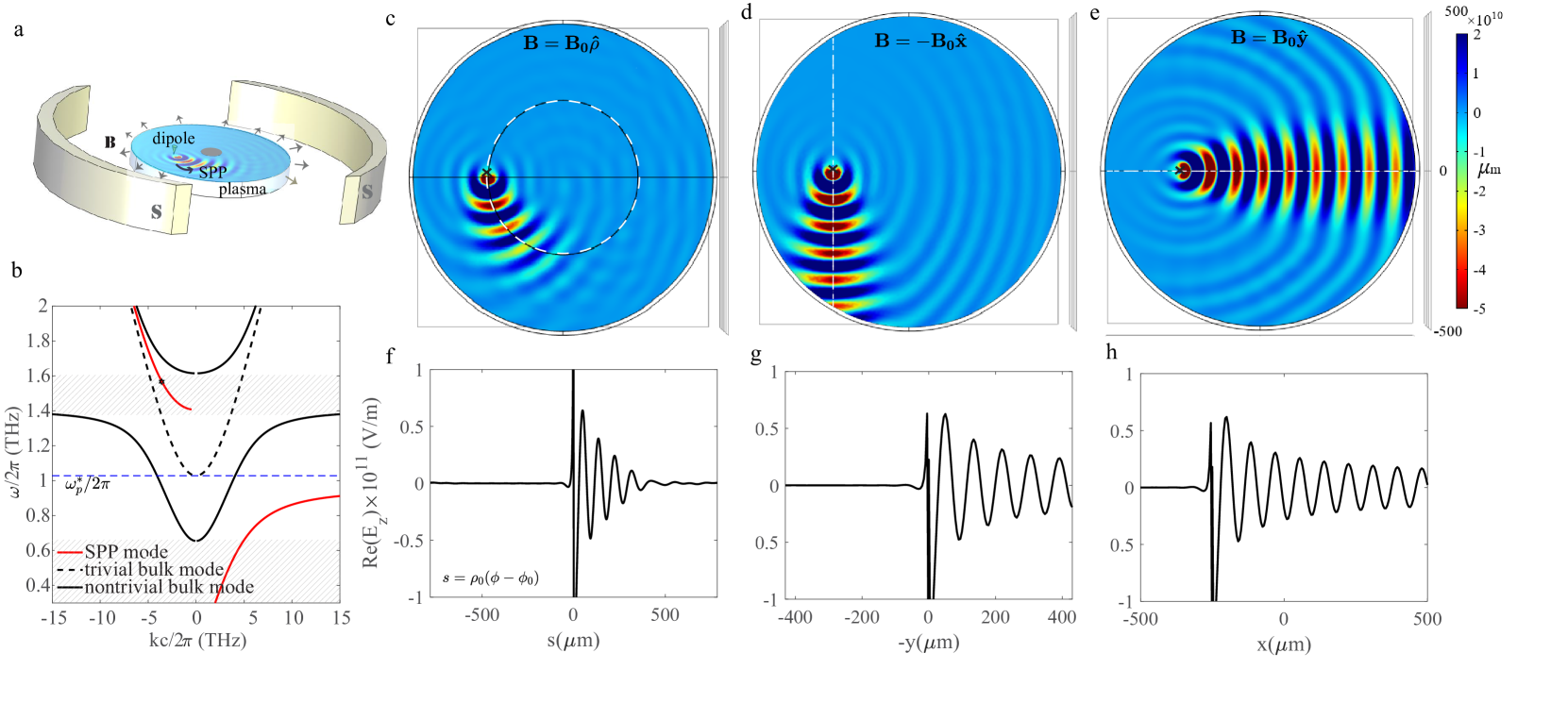
Figure 1: Unidirectional curved SPP vs. linear propagating SPP. (a) Geometry sketch (b) Bulk and SPP dispersion diagrams. The gray regions denote the band gaps. The electric field profile ($E_{z}$) of the SPP propagating at the interface of an isotropic medium and a plasma region magnetized by (c) a static radial bias $\mathbf{B}=B_{0}\mathbf{\hat{\rho}}$ that is centered on the origin, (d) an axial bias $\mathbf{B}=-B_{0}\mathbf{\hat{x}}$, and (e) an axial bias $\mathbf{B}=B_{0}\mathbf{\hat{y}}$. The SPPs are excited by a point source located at $(\rho_{0},\phi_{0},z)=(250\mu\text{m},\pi,0)$. (f,g,h) The electric field oscillation, respectively along the circular, vertical and horizontal trajectories shown by white dashed lines in (c,d,e). In (f), s is the arc length defined as $s=\rho_{0}cos(\phi-\phi_{0})$ where $\phi$ is the angle of the observation point with respect to the x-axis and $\rho_{0}$ is the radius of the dashed circle. The magnetized plasma is characterized by (1) where $n_{e}=3.6\times 10^{21}\text{m}^{-3},m^{\ast}=0.0175m_{0},\varepsilon_{\infty}=15.68,B_{0}=0.6\text{T}$, given $\omega_{p}^{\ast}=\omega_{p}/\sqrt{\varepsilon_{\infty}}=2\pi(1.03\text{THz}),\omega_{c}/\omega_{p}^{\ast}=0.93$ and $\Gamma=0.00015\omega_{p}$. The top region is metal with dielectric constant of $\varepsilon_{r}=-10^{4}$. The resonance frequency $f=1.567\text{THz}$ is within the upper band gap.

Consider a plasma medium consisting of $n_{e}$ free electrons with the effective mass of $m^{\ast}$ per volume, which is magnetized by a static magnetic field bias $\mathbf{B}_{c}=B_{0}\mathbf{\hat{b}}_{c}$ where $B_{0}$ is the magnetic field strength and $\mathbf{\hat{b}}_{c}$ is a unit vector along the direction of the magnetic field. In general, the material is characterized by a dielectric tensor [34]

$$\mathbf{\bar{\varepsilon}=}\varepsilon_{t}(\mathbf{\bar{I}-\hat{b}}_{c}\mathbf{\hat{b}}_{c})+i\varepsilon_{\text{g}}(\mathbf{\hat{b}}_{c}\times\mathbf{\bar{I}})+\varepsilon_{\text{a}}\mathbf{\hat{b}}_{c}\mathbf{\hat{b}}_{c}$$ (1)

where the permittivity elements are defined using a Drude model as

$$\varepsilon_{t}=\varepsilon_{\infty}-\frac{\omega_{p}^{2}(1+i\Gamma/\omega)}{(\omega+i\Gamma)^{2}-\omega_{c}^{2}},\text{ \ }\varepsilon_{a}=\varepsilon_{\infty}-\frac{\omega_{p}^{2}}{\omega(\omega+i\Gamma)},\text{ \ }$$

$$\varepsilon_{g}=\frac{\omega_{c}\omega_{p}^{2}}{\omega\left[\omega_{c}^{2}-(\omega+i\Gamma)^{2}\right]},$$ (2)

assuming the time harmonic variation of $e^{-i\omega t}$; $\omega_{p}=$ $\sqrt{n_{e}q_{e}^{2}/(m^{\ast}\varepsilon_{0})}$, $\omega_{c}=$ $-q_{e}B_{0}/m^{\ast}$ and $\Gamma=-q_{e}/\mu m^{\ast}$ are plasma, cyclotron, and collision frequencies, respectively, $q_{e}$ is the electron charge, $\varepsilon_{\infty}$ is high-frequency dielectric constant, and $\mu$ is the carrier mobility. In this work, we apply a uniform radial bias, $\mathbf{B}_{c}=B_{0}\mathbf{\hat{\rho}}$ to magnetize the plasma region. Figure 1a illustrates the geometry scheme of the system under study. It includes a plasma slab under radial bias, covered by an isotropic material. The radial bias can be practically implemented using concave permanent magnets. We assume that the plasma thickness is large, then the system is two half-spaces of gyrotropic/isotropic media. The plasma region is model by (1), where $\mathbf{\hat{b}}_{c}=\mathbf{\hat{\rho}}$ and $\mathbf{\bar{I}}$ is a dyadic tensor in polar coordinates with ($\mathbf{\hat{\rho},\hat{\phi},\hat{z}}$) unit basis. Next, we study the properties of the bulk modes propagating inside the radially magnetized plasma region. Then, we look for the SPPs excited at the interface of the isotropic/radially magnetized plasma media.

A plane wave propagating in the gyrotropic medium with the wave vector $\mathbf{k}=k_{\rho}\mathbf{\hat{\rho}}^{\prime}\mathbf{+}k_{z}\mathbf{\mathbf{\hat{z}}}$ satisfies the wave equation $\mathbf{k}\times\left(\mathbf{k\times E}\right)+k_{0}^{2}\mathbf{\bar{\varepsilon}}_{r}\cdot\mathbf{E=0}$. The non-zero solution of $\mathbf{E}$ exists only if $\left|k_{0}^{2}\mathbf{\bar{\varepsilon}}_{r}-k^{2}\mathbf{\bar{I}}+\mathbf{kk}\right|=0$. This determinant is the dispersion equation of the bulk modes propagating with an arbitrary direction in a gyrotropic medium. Consider an orthogonal coordinate system, having a unit vector along the magnetic bias as $\left\{\mathbf{\hat{k}}_{t},\mathbf{\hat{\rho},\hat{k}}_{t}\times\mathbf{\hat{\rho}}\right\}$. The wave vector in this coordinate is rewritten as $\mathbf{k=k}_{t}+q_{\rho}\mathbf{\hat{\rho}}$ with $\mathbf{k}_{t}=q_{\varphi}\mathbf{\hat{\phi}+}k_{z}\mathbf{\hat{z}}$, where $q_{\rho}=k_{\rho}\cos(\phi_{\mathbf{k}}-\phi_{\mathbf{b}})$ and $q_{\varphi}=k_{\rho}\sin(\phi_{\mathbf{k}}-\phi_{\mathbf{b}})$; $\phi_{\mathbf{k}}$ and $\phi_{\mathbf{b}}$ are the angle of the wave and bias vectors with respect to the $x$-axis, respectively. By plugging $\mathbf{\bar{\varepsilon}}$ and $\mathbf{k}$ into the above determinant, we derive

$$k_{t}^{2}=\frac{1}{2\varepsilon_{t}}\left[-\kappa\pm\sqrt{\kappa^{2}-4\varepsilon_{t}\nu}\right]\text{,}$$ (3)

where $\kappa=q_{\rho}^{2}(\varepsilon_{t}+\varepsilon_{a})+k_{0}^{2}\left(\varepsilon_{g}^{2}-\varepsilon_{t}(\varepsilon_{t}+\varepsilon_{a}\right))$, $\nu=\varepsilon_{a}\left(q_{\rho}^{2}-k_{0}^{2}\varepsilon_{t}\right)^{2}-\varepsilon_{a}\varepsilon_{g}^{2}k_{0}^{4}$, and $k_{t}^{2}=q_{\varphi}^{2}+k_{z}^{2}$. We look for the bulk modes propagating perpendicular to the bias. Thus, we set $q_{\rho}=0$ in (3) and determine two equations as $k_{1}^{2}=\varepsilon_{\text{eff}}k_{0}^{2}$ and $k_{2}^{2}=\varepsilon_{\text{a}}k_{0}^{2}$ where $\varepsilon_{\text{eff}}=(\varepsilon_{t}^{2}-\varepsilon_{g}^{2})/\varepsilon_{t}$, $\ k_{0}$ is the free space wave number, and $k_{j}^{2}=q_{\varphi}^{2}\mathbf{+}k_{zj}^{2}$, $j\in\left\{1,2\right\}$. These equations characterize the nontrivial TM modes with $E_{\varphi},E_{z},H_{\rho}$ (no electric field component along the bias vector) and trivial TE modes with $H_{\varphi},H_{z},E_{\rho}$ (no magnetic field component along the bias), respectively. The nontrivial modes are dependent to the magnetic bias, unlike the trivial modes. Note that in a cylindrical rode pure TE and pure TM modes exist only when the field configurations are symmetric and independent of $\phi$. Here, nontrivial TM and trivial TE modes have phase variation of $\exp(im\varphi)$. Therefore, they cannot be pure TE and TM modes; they are hybrid modes. A wave with $q_{\rho}=0$ is a traveling wave on a cylindrical shell, which can be decomposed into nontrivial TM and trivial TE modes in a radially magnetized system. It has a vortex-like behavior and its phase varies as $\exp(im\varphi)$. An electromagnetic vortex is a differentiated plane wave which can be generated by three homogeneous plane wave interference [35, 36].

Next, by enforcing continuity of the tangential components of the electric and magnetic fields of these particular bulk modes at the interface, we derive the SPP dispersion equation as

$$\frac{\sqrt{k_{s}^{2}-k_{0}^{2}\varepsilon_{r}}}{\varepsilon_{r}}+\frac{\sqrt{k_{s}^{2}-k_{0}^{2}\varepsilon_{\text{eff}}}}{\varepsilon_{\text{eff}}}=\frac{\varepsilon_{g}k_{s}}{\varepsilon_{t}\varepsilon_{\text{eff}}},$$ (4)

where $k_{s}=q_{\varphi}$ is the propagation constant of the surface wave and $\varepsilon_{r}$ is the effective permittivity of the isotropic region. This dispersion relation is the same as for axial bias in the Voight configuration. Figure 1b shows the dispersion diagrams of the nontrivial TM, trivial TE bulk modes, and the SPP modes. The shaded gray regions indicate bandgaps between the nontrivial bulk bands. Like usual topological plasma systems when an axial bias is applied, the SPPs crossing the nontrivial bandgaps are potentially topological. Their frequency response is asymmetric.

Then, We have simulate the system under study using COMSOL Multiphysics. The plasma region is characterized by parameters presented in [37, 38], and provided in the caption of Fig. 1, related to an undoped InSb crystal at moderate temperatures. The SPPs are excited by a point source located at the interface of the gyrotropic/isotropic media, operating at a frequency within the upper nontrivial bandgap. The electric field profile at the interface is shown in Fig. 1c. It shows the SPPs propagating counter clock-wise (CCW) on a circular path about the origin. There is no propagation in the opposite direction due to the unidirectional nature of the wave. So, the excited SPPs have a circular trajectory rather than a linear trajectory as a result of applying the radial bias.

For comparison, we obtain the field profile of the SPPs when the axial biases $\mathbf{\hat{b}}_{c}=-\mathbf{\hat{x}}$ and $\mathbf{\hat{b}}_{c}=\mathbf{\hat{y}}$ are applied (the usual cases). The results are shown in Figs. 1d and 1e. Here, the unidirectional SPPs have linear propagation. They are characterized by the same dispersion equation as Eq. 4, but with surface momentum $k_{s}=-q_{y}$ and $k_{s}=q_{x}$, respectively. Comparing Fig. 1c with Fig. 1d and Fig. 1e, the deviation of the SPPs from a straight line to a circular path is evident. In all cases, the SPPs tend to propagate perpendicular to the static bias. For that reason, in the radial bias system the surface plasmons gain orbital angular momentum and form curved SPPs.

The line graphs in Fig. 1f,g,h indicate the electric field oscillation along the circular, vertical and horizontal straight line traces shown by white dashed lines in the field profile plots. According to the period of the oscillation, the SPP wavelength for radial and axial bias cases are almost equal ($\lambda_{SPP}\simeq 84\mu m$). The obtained wavelength is consistent with the estimated value obtained from the dispersion diagram ($\lambda_{SPP}=2\pi/\text{Re}(k_{s})$). The SPPs have similar propagation properties, however, the decay rate of the curved SPP is much higher. We find that the curved SPPs are leaky modes, while the linear SPPs in the axially biased systems are confined propagating modes. The difference in results is due to the hybrid nature of the nontrivial and trivial bulk modes in the radially biased system. In fact, the curved SPPs excited at a resonance frequency within the upper nontrivial bandgap can be coupled to the trivial TE cylindrical bulk modes. This does not occur in an axially biased system, because in that case the trivial TE and nontrivial TM modes are orthogonal modes, and hence, the TE modes do not contribute to the excitation of the TM SPP. Consequently, the TM SPPs are confined modes at frequencies within the nontrivial bandgaps and their energy does not couple to the trivial TE mode.

III Dyadic Green’s Function for a radially magnetized plasma

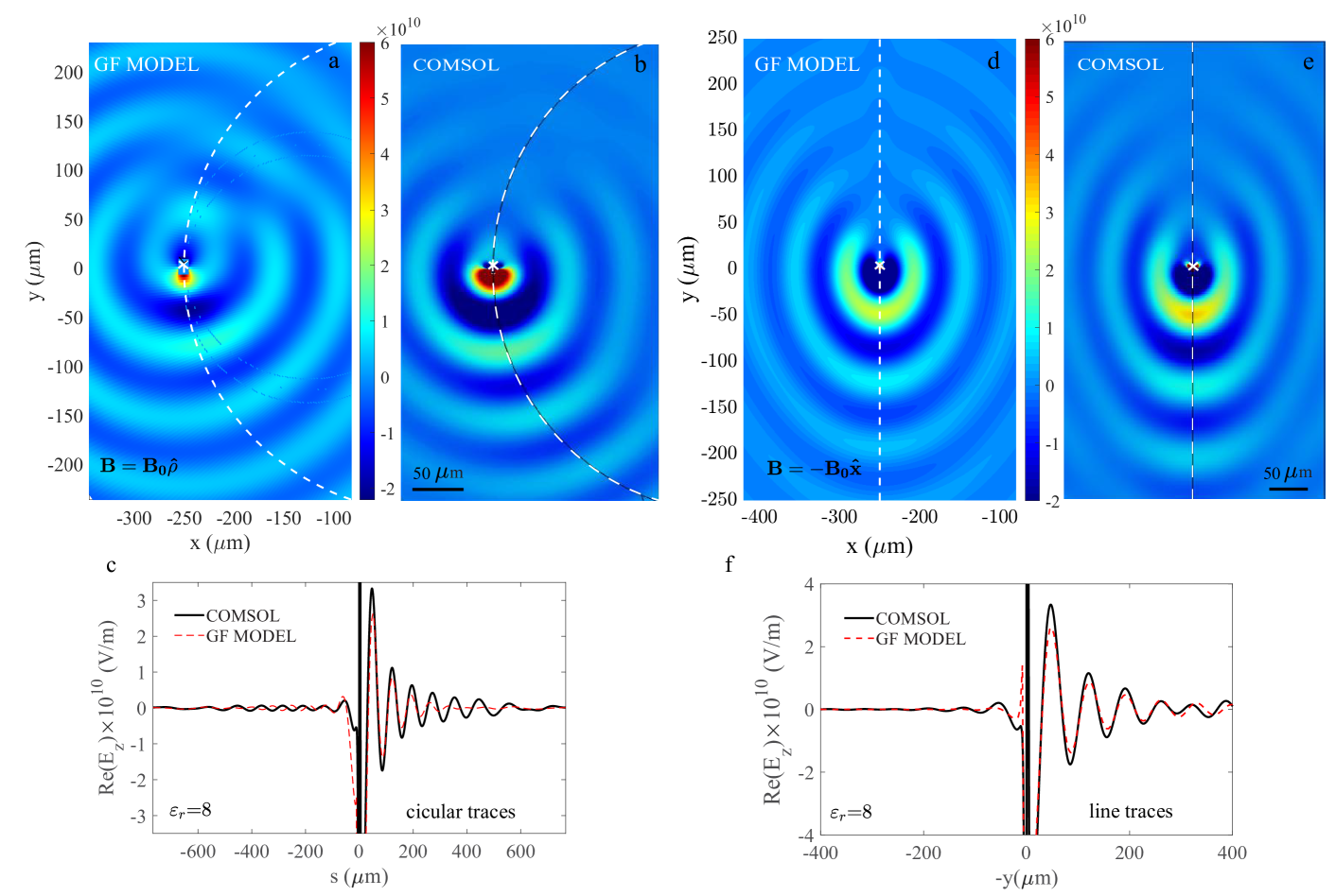
Figure 2: Electric field distribution ($E_{z}$) of the curved SPPs excited at the interface of dielectric/ radially magnetized plasma ($\mathbf{B}=B_{0}\mathbf{\hat{\rho}}$) media using (a) Green’s function model (14) and (b) a full-wave COMSOL simulation. The radial bias is centered on the origin and the dipole is located at $(250\mu\text{m},\pi,0)$. The observation points are on a plane with distance $z=0.003\lambda_{p}$ above the interface ($\lambda_{p}=2\pi/\omega_{p}$). (c) The electric field oscillation along the circular trajectories (white dashed semicircles). The electric field profile of the linear propagating SPPs excited at the interface of the dielectric/axially biased plasma ($\mathbf{B}=-B_{0}\mathbf{\hat{x}}$) using (d) GF model (e) COMSOL simulation. (f) The extracted data from dashed line trajectories. The magnetized plasma is characterized by (1) where $n_{e}=3.6\times 10^{21}\text{m}^{-3},m^{\ast}=0.0175m_{0},\varepsilon_{\infty}=15.68,B_{0}=0.6\text{T}$ and $\Gamma=0.00015\omega_{p}$. The dielectric constant of top region is $\varepsilon_{r}=8$. The resonance frequency is $f=1.567\text{THz}$.

Here, we analytically obtain the electric field of the curved SPPs in a radially magnetized system. They are excited by a point source at the interface of two half-space media where the $z<0$ region is filled by a radially magnetized plasma and the $z>0$ region is an isotropic material. The radial bias is centered on the origin and the dipole is located inside the isotropic region at $\mathbf{r}_{0}=(\rho_{0},\phi_{0},d)$. By doing a Green’s function (GF) analysis in a polar coordinate system, the tangential and normal components of the scattered field in the isotropic region at $\mathbf{r}=(\rho,\phi_{\mathbf{r}},z)$ due to a vertical dipole source with moment of $\mathbf{p=}\gamma\mathbf{\hat{z}}$ are governed by

$$\mathbf{E}_{||}^{s}(\mathbf{r})=\frac{1}{(2\pi)^{2}}\int_{0}^{\infty}\int_{0}^{2\pi}\mathbf{\bar{R}(q)\cdot}i\mathbf{q}\frac{\gamma e^{-\gamma_{0}(z+d)}}{2\varepsilon_{r}\varepsilon_{0}}e^{i\mathbf{q}\cdot\left(\mathbf{r}-\mathbf{r}_{0}\right)}qd\phi_{\mathbf{q}}dq$$ (5)

and

$$E_{z}^{s}(\mathbf{r})=\frac{-1}{(2\pi)^{2}}\int_{0}^{\infty}\int_{0}^{2\pi}C^{r}(\mathbf{q})\frac{\gamma e^{-\gamma_{0}(z+d)}}{2\gamma_{0}\varepsilon_{r}\varepsilon_{0}}e^{i\mathbf{q}\cdot\left(\mathbf{r}-\mathbf{r}_{0}\right)}qd\phi_{\mathbf{q}}dq$$ (6)

where $C^{r}(\mathbf{q})=\mathbf{q}\cdot\mathbf{\bar{R}(q)\cdot q}$ and $\mathbf{\bar{R}(q)}$ is a 2x2 reflection coefficient. The GF derivation details and quantities are defined in the appendix. Using these 2D Sommerfeld integrals, the field computation is very time consuming and it does not converge well. To solve this problem, we use a saddle point approximation and simplify (6) to a 1D integral as defined in (15). Then, using this Green’s function model, we generate the field density profile shown in Fig. 2a by computing the electric field of the observation points on a plane above the interface with local position ($\rho,\phi_{\mathbf{r}},z=0.003\lambda_{p}$), where $\lambda_{p}=2\pi/\omega_{p}$. The top region is a dielectric with $\varepsilon_{r}=8$. The plot shows one-way SPPs with CCW propagation on a circular path. For comparison, we generated Fig. 2b based on a numerical computation using COMSOL. The GF result is consistent with the numerical result. Then, the data are extracted from the circular traces shown by white dashed lines to generate the line graph in Fig. 2c. As shown, the results arising from the GF model are very close to the COMSOL results, which validates the accuracy of our GF model for radially biased system.

We also develop the GF model presented in [39, 40] for an axial bias along the $-x$ direction. For this case, the SPPs are propagating along a straight line. Figure 2d and 2e demonstrate the electric field density and Fig. 2g shows the SPP oscillation along the dashed line trajectories using axial GF model and COMSOL simulation.

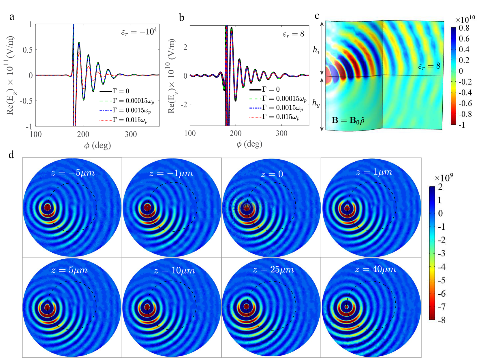
Figure 3: (a,b) Unidirectional curved SPPs by considering different amounts of dissipation (metal or dielectric on top) (c) A vertical cross-section view of the two-layer magnetized system ($h_{i}=h_{g}=200\mu\text{m}$). Energy leakage occurs in the dielectric region after several wavelengths of curved SPP propagation (d) Electric field density of the curved SPPs on the surfaces parallel to the interface located at different distances (z) from the interface $z=0$ ($\varepsilon_{r}=8$). $n_{e}=3.6\times 10^{21}\text{m}^{-3},m^{\ast}=0.0175m_{0},\varepsilon_{\infty}=15.68,B_{0}=0.6\text{T}$, $f=1.567\text{THz}$.

Figure 3a,b shows the unidirectional curved SPP oscillation along the circular path in the radially magnetized system by considering different amounts of dissipation when the top region is metal or dielectric. As shown, by reducing the loss, the magnitude increases and the curved SPPs propagate longer, as expected. However, even in a loss-less system the SPPs do not rotate on a full circle. They stop their orbital propagation on the surface after several SPP wavelengths of propagation and they radiate to the plasma or dielectric region. The leakage to the dielectric is illustrated in Fig. 3c, showing a vertical cross section of the system (including the dielectric and the radially magnetized plasma); a cut cylinder that is intersected by a plane. The curved SPP is leaky for this operating frequency, as discussed in Section I. In addition, for the case of dielectric on top, the mode lies within the light cone of the dielectric region. Figure 3d shows the electric field profile on surfaces parallel to the interface, located at different heights below and above the interface. In the plasma region and close to the surface, the SPPs spiral on a circle centered at the origin. In the dielectric region, they remain on this path at distances close to the interface. Moving farther vertically from the interface, SPPs spiral out of the circle. We also observed that SPPs are more confined to the surface when the top layer is a metal.

IV An application for curved SPPs

Waveguide bends connecting two straight waveguides are important components in plasmonic integrated circuits. Using unidirectional curved SPPs, a bent waveguide with minimal bending loss can be designed. We propose that a 90-degree circular bend magnetized by a radial bias can be used as a nonreciprocal plasmonic junction. As shown in Fig. 4a, the excited unidirectional SPPs steer from a straight line to a circular path through the 90 degree bend, resulting in reduction of the radiation loss due to the curvature of the waveguide junction. Black arrows indicate the magnetic bias vectors applied in each segment. It forms an optical nonreciprocal plasmonic junction, which allows power transmission only in one direction.

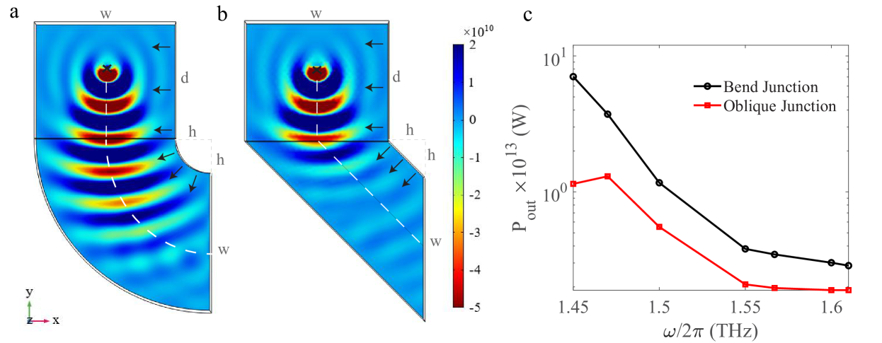
Figure 4: Electric field profile of the SPP propagating at the interface of metal/magnetized plasma, passing through (a) a $90^{\circ}$ circular bend junction under radial bias vs. (b) an oblique junction under $5\pi/4$ axial bias. (c) Output power vs. frequency. $n_{e}=3.6\times 10^{21}\text{m}^{-3},m^{\ast}=0.0175m_{0},\varepsilon_{\infty}=15.68,B_{0}=0.6\text{T}$, $\Gamma=0.00015\omega_{p}$, $\varepsilon_{r}=-10^{4}$, $f=1.567\text{THz},w=4h=360\mu\text{m},d=300\mu\text{m}.$

To provide a comparison to the axial-bias case, in Fig. 4b, two straight waveguides are connected by an oblique junction magnetized by an axial bias with angle of $5\pi/4$ radian. When unidirectional SPPs reach the input port of the oblique junction, they change direction and align themselves along a line perpendicular to the bias. That is because the unidirectional SPPs inherently tend to propagate perpendicular to the magnetic bias at frequencies within the nontrivial bandgap.

The surface power that flows through these two junctions are computed at the output ports for different operating frequencies within the upper bandgap and shown in Fig. 4c. The power is transmitted through the radially magnetized circular bend more than two times higher than the power transmitted through the oblique junction. In addition, the power transmission is significantly higher than an unbiased circular junction. In the circular bend with radial bias, the energy routing only occurs in one direction. By reversing the magnetic field direction, the energy is routed in the opposite direction.

V Conclusion

In conclusion, we obtained unidirectional curved SPPs by applying an in-plane radial magnetic bias in topological continua. In a magnetized system, the unidirectional SPP trajectories are steerable by the magnetic bias direction. We derived a Green’s function model for a radially magnetized system. The properties of unidirectional curved SPPs were compared to the linear SPP. Using unidirectional curved SPPs, a bent waveguide with minimal bending loss and nonreciprocal features was proposed for plasmonic integrated circuits.

VI Appendix

Here, we obtain the scattered field in a radially biased system based on a Green’s function analysis in polar coordinates. Consider two half-space isotropic/magnetized plasma media having an interface at $z=0$. An electric source with dipole moment of $\mathbf{p=}\gamma\mathbf{\hat{z}}$ is located at $\mathbf{r}_{0}=(\rho_{0},\phi_{0},d)$ in the isotropic region. The primary electric and magnetic fields are $\mathbf{E}^{p}(\mathbf{r})=(\varepsilon_{r}k_{0}^{2}\mathbf{I+\nabla\nabla})\cdot\mathbf{\pi}^{p}$ and $\mathbf{H}^{p}(\mathbf{r})=i\omega\varepsilon_{0}\varepsilon_{r}\mathbf{\nabla}\times\mathbf{\pi}^{p}$, where the Hertzian potential $\mathbf{\pi}^{p}$ is given by $\mathbf{\pi}^{p}(\mathbf{r})=g^{p}(\mathbf{r,r}_{0})\mathbf{p/}\varepsilon_{r}\varepsilon_{0}$. The primary Green’s function is

$$g^{p}(\mathbf{r,r}_{0}) = \frac{e^{-i\sqrt{\varepsilon_{r}}k_{0}\left|\mathbf{r-r}_{0}\right|}}{4\pi\left|\mathbf{r-r}_{0}\right|}$$

$$= \frac{1}{(2\pi)^{2}}\int_{0}^{\infty}\int_{0}^{2\pi}\frac{e^{-\gamma_{0}\left|z-d\right|}}{2\gamma_{0}}e^{i\mathbf{q}\cdot\left(\mathbf{r}-\mathbf{r}_{0}\right)}qd\phi_{\mathbf{q}}dq$$

where $\mathbf{q}\cdot\mathbf{r}=q\rho\cos(\phi_{\mathbf{q}}-\phi_{\mathbf{r}})$ and $\mathbf{q}\cdot\mathbf{r}_{0}=q\rho_{0}\cos(\phi_{\mathbf{q}}-\phi_{0})$ with $\left\{\phi_{\mathbf{q}},\phi_{\mathbf{r}},\phi_{0}\right\}$ denoting the angles $\mathbf{q}$, $\mathbf{r}$, and $\mathbf{r}_{0}$ make with the Cartesian unit vector $\mathbf{\hat{x}}$. The exponential factor is $\gamma_{0}=\sqrt{q^{2}-\varepsilon_{r}k_{0}^{2}}$, where $\varepsilon_{r}$ is the dielectric constant of the isotropic region ($z>0$). Using the Fourier transform pairs and nabla relations in a polar coordinate, we have

$$\mathbf{E}^{p}(\mathbf{r}) = \frac{\gamma g^{p}(\mathbf{r,r}_{0})}{\varepsilon_{r}\varepsilon_{0}}\left[\mathbf{\nabla}_{t}\partial_{z}+\left(\frac{\partial^{2}}{\partial z^{2}}+\varepsilon_{r}k_{0}^{2}\right)\mathbf{\mathbf{\hat{z}}}\right]$$ (8)

$$\mathbf{E}^{p}(z,\mathbf{q}) = \mathbf{E}_{||}^{p}+E_{z}^{p}\mathbf{\mathbf{\hat{z}}}$$ (9)

$$= \frac{\gamma g^{p}(z\mathbf{,q})}{\varepsilon_{r}\varepsilon_{0}}\left[i\mathbf{q}\partial_{z}+\left(\frac{\partial^{2}}{\partial z^{2}}+\varepsilon_{r}k_{0}^{2}\right)\mathbf{\mathbf{\hat{z}}}\right]$$

where $g^{p}(z\mathbf{,q})=e^{-i\mathbf{q}\cdot\mathbf{r}_{0}}e^{-\gamma_{0}\left|z-d\right|}/2\gamma_{0}$. The total field in the isotropic region is a superposition of the primary and scattered field, $\mathbf{E}^{(1)}(\mathbf{r})=\mathbf{E}^{p}(\mathbf{r})+\mathbf{E}^{s}(\mathbf{r})$. Let $\mathbf{\bar{R}}$ be a reflection tensor such that the tangential components of the scattered field at the interface are related to the tangential primary field as

$$\mathbf{E}_{||}^{s}(z\mathbf{,q})=\mathbf{E}_{||}^{s}(\mathbf{q})e^{-\gamma_{0}z}=\mathbf{\bar{R}(\mathbf{q})\cdot E}_{||}^{p}(0\mathbf{,q})e^{-\gamma_{0}z}.$$ (10)

Substitution of (9) gives

$$\mathbf{E}_{||}^{s}(z\mathbf{,q})=\mathbf{\bar{R}(q)}\cdot i\mathbf{q}\frac{\gamma}{2\varepsilon_{r}\varepsilon_{0}}e^{-\gamma_{0}(z+d)}e^{-i\mathbf{q}\cdot\mathbf{r}_{0}}.$$ (11)

According to the Gauss’s law for the scattered field $\mathbf{\nabla}\cdot\mathbf{E}^{s}=0$, the $z$ component of the scattered field is $E_{z}^{s}(\mathbf{r})=-\int\mathbf{\nabla}_{t}\cdot\mathbf{E}_{||}^{s}(\mathbf{r})dz$. Using (11) we have,

$$E_{z}^{s}(z\mathbf{,q}) = -i\mathbf{q}\cdot\mathbf{E}_{||}^{s}(\mathbf{q})\int e^{-\gamma_{0}z}dz$$ (12)

$$= \frac{-\gamma}{2\varepsilon_{r}\varepsilon_{0}\gamma_{0}}\mathbf{q}\cdot\mathbf{\bar{R}(q)\cdot q}e^{-\gamma_{0}(z+d)}e^{-i\mathbf{q}\cdot\mathbf{r}_{0}}.$$

Finally, by taking the spatial Fourier transform we have

$$\mathbf{E}_{||}^{s}(\mathbf{r})=\frac{1}{(2\pi)^{2}}\int_{0}^{\infty}\int_{0}^{2\pi}\mathbf{\bar{R}(q)}\cdot i\mathbf{q}\frac{\gamma e^{-\gamma_{0}(z+d)}}{2\varepsilon_{r}\varepsilon_{0}}e^{i\mathbf{q}\cdot\left(\mathbf{r}-\mathbf{r}_{0}\right)}qd\phi_{\mathbf{q}}dq$$ (13)

and

$$E_{z}^{s}(\mathbf{r})=\frac{1}{(2\pi)^{2}}\int_{0}^{\infty}\int_{0}^{2\pi}C^{r}(\mathbf{q})\frac{-\gamma}{\varepsilon_{r}\varepsilon_{0}}\frac{e^{-\gamma_{0}(z+d)}}{2\gamma_{0}}e^{i\mathbf{q}\cdot\left(\mathbf{r}-\mathbf{r}_{0}\right)}qd\phi_{\mathbf{q}}dq$$ (14)

where $C^{r}(\mathbf{q})=\mathbf{q}\cdot\mathbf{\bar{R}(q)\cdot q}$. Using the saddle point approximation, the last 2D Sommerfeld integral can be simplified as

$$E_{z}^{s}(\mathbf{r})=\int_{0}^{\infty}I(q)\frac{-\gamma e^{-\gamma_{0}(z+d)}}{2\varepsilon_{r}\varepsilon_{0}\gamma_{0}}qdq$$ (15)

where

$$I(q)=\frac{1}{(2\pi)^{2}}\sqrt{\frac{\pi}{2q\left|g(\phi_{\mathbf{s}})\right|}}\left[C^{r}(q,\phi_{\mathbf{s}})e^{iqg(\phi_{\mathbf{s}})}e^{i\pi\varsigma/4}\right.$$

$$\left.+C^{r}(q,\phi_{\mathbf{s}}-\pi)e^{-iqg(\phi_{\mathbf{s}})}e^{-i\pi\varsigma/4}\right]$$ (16)

with $g(\phi_{\mathbf{s}})=\rho\cos(\phi_{\mathbf{s}}-\phi_{\mathbf{r}})-\rho_{0}\cos(\phi_{\mathbf{s}}-\phi_{0})$, $\varsigma$ is the sign of $g"(\phi_{\mathbf{s}})$, and the saddle point is

$$\phi_{\mathbf{s}}=\tan^{-1}\left(\frac{\rho_{0}\sin(\phi_{0})-\rho\sin(\phi_{\mathbf{r}})}{\rho_{0}\cos(\phi_{0})-\rho\cos(\phi_{\mathbf{r}})}\right)$$ (17)

where $\phi_{\mathbf{s}}\in(0,\pi)$. Figure 5 shows that the approximated relation is matched with the exact solution.

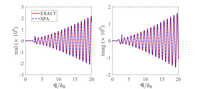
Figure 5: Saddle point approximation vs. exact solution (the integrand of (15) and (14), respectively, over $q$ variation) for $f=1.567\text{THz}$ at ($\rho=250\mu\text{m},\phi=5\pi/4,z=0.003\lambda_{p}$). $n_{e}=3.6\times 10^{21}\text{m}^{-3},m^{\ast}=0.0175m_{0},\varepsilon_{\infty}=15.68,B_{0}=0.6\text{T}$, and $\varepsilon_{r}=8$.

VI-A Reflection Tensor in a radially biased system

A plane wave in a gyrotropic medium satisfies the wave equation $\mathbf{k}\times\left(\mathbf{k\times E}\right)+k_{0}^{2}\mathbf{\bar{\varepsilon}}_{r}\cdot\mathbf{E=0}$. Consider a coordinate system, having a unit vector along the magnetic bias $\left\{\mathbf{\hat{k}}_{t},\mathbf{\hat{\rho},\hat{k}}_{t}\times\mathbf{\hat{\rho}}\right\},$ where $\mathbf{k=k}_{t}+q_{\rho}\mathbf{\hat{\rho}}$ with $\mathbf{k}_{t}=q_{\varphi}\mathbf{\hat{\phi}+}k_{z}\mathbf{\hat{z}}$. We define $q_{\rho}\equiv k_{\rho}\cos(\phi_{\mathbf{k}}-\phi_{b})$ and $q_{\varphi}\equiv k_{\rho}\sin\phi_{\mathbf{k}}-\phi_{b})$ where $q_{\rho},q_{\varphi}\in\left[-\infty,\infty\right]$. Note that the permittivity tensor is given in ($\mathbf{\hat{\rho},\hat{\phi},\hat{z}}$) polar basis which is related to ($\mathbf{\hat{\rho}{\acute{}},\hat{\phi}{\acute{}},\hat{z}}$) basis by projection relations of $\mathbf{\hat{\rho}{\acute{}}\cdot\hat{\rho}}\mathbf{=}\cos(\phi_{\mathbf{k}}-\phi_{b})$ and $\mathbf{\hat{\rho}{\acute{}}\cdot\hat{\phi}}\mathbf{=}\sin(\phi_{\mathbf{k}}-\phi_{b})$. Also, the permittivity elements are not spatially dependent. In the wave equation, the non-zero solution of $\mathbf{E}$ exists only if $\left|k_{0}^{2}\mathbf{\bar{\varepsilon}}_{r}-k^{2}\mathbf{\bar{I}}+\mathbf{kk}\right|=0$. The determinant is a general relation for dispersion equation of the bulk modes propagating in a gyrotropic medium in any arbitrary direction. By plugging $\mathbf{\bar{\varepsilon}}_{r}$ tensor and $\mathbf{k}$ into the dispersion relation, we obtain two solutions for $k_{z}$ as

$$k_{zj}=\sqrt{-q_{\varphi}^{2}+\frac{1}{2\varepsilon_{t}}\left[-\kappa\pm\sqrt{\kappa^{2}-4\varepsilon_{t}\nu}\right]}$$ (18)

for $j\in\left\{1,2\right\}$ where

$$\kappa = q_{\rho}^{2}(\varepsilon_{t}+\varepsilon_{a})+k_{0}^{2}\left(\varepsilon_{g}^{2}-\varepsilon_{t}(\varepsilon_{t}+\varepsilon_{a}\right)$$ (19)

$$\nu = \varepsilon_{a}\left(q_{\rho}^{2}-k_{0}^{2}\varepsilon_{t}\right)^{2}-\varepsilon_{a}\varepsilon_{g}^{2}k_{0}^{4}.$$ (20)

Hence, the field in the gyrotropic region ($z<0$) can be written as a superposition of two waves with the wave vectors $\mathbf{k}_{j}=\mathbf{k}_{tj}+q_{\rho}\mathbf{\hat{\rho}}$ where $\mathbf{k}_{tj}=$ $q_{\varphi}\mathbf{\hat{\phi}}+k_{zj}\mathbf{\hat{z}}$. The electric field vector in the selected coordinate is written as $\mathbf{E}_{j}=\mathbf{E}_{0j}e^{i\mathbf{k}_{j}\cdot\mathbf{r}}=\left[\alpha_{1}\mathbf{\hat{k}}_{tj}+\alpha_{2}\mathbf{\hat{\rho}}+\alpha_{3}\left(\mathbf{\hat{k}}_{tj}\times\mathbf{\hat{\rho}}\right)\right]e^{i\mathbf{k}_{j}\cdot\mathbf{r}}$. By plugging $\mathbf{E,}$ $\mathbf{k}$ and $\mathbf{\bar{\varepsilon}}_{r}$ into the wave equation, the unknown coefficients $\alpha_{i}$ are obtained. Then we have

$$\mathbf{E}_{0}\sim\mathbf{k}_{tj}+q_{\rho}\theta_{j}\mathbf{\hat{\rho}}+\Delta_{j}\left(\mathbf{k}_{tj}\times\mathbf{\hat{\rho}}\right)$$ (21)

where

$$\Delta_{j}\equiv\frac{i\varepsilon_{\text{g}}k_{0}^{2}}{\varepsilon_{\text{t}}k_{0}^{2}-k_{j}^{2}}\text{, \ \ \ }\theta_{j}\equiv\frac{-k_{tj}^{2}}{\varepsilon_{\text{a}}k_{0}^{2}-k_{tj}^{2}}$$ (22)

and the magnetic field is $\mathbf{H}=\left(\mathbf{k}\times\mathbf{E}\right)/\omega\mu_{0}$. In the isotropic region, the field can be expanded as $\mathbf{E}=\left[B_{1}\left(\mathbf{k}_{d}\times\mathbf{\hat{z}}\right)+B_{2}\mathbf{k}_{d}\times\left(\mathbf{k}_{d}\times\mathbf{\hat{z}}\right)\right]e^{i\mathbf{k}_{d}\cdot\mathbf{r}}$ where $\mathbf{k}_{d}=q_{\rho}\mathbf{\hat{\rho}}+q_{\varphi}\mathbf{\hat{\phi}}+k_{zd}\mathbf{\hat{z}}$ and $k_{d}=k_{0}^{2}\varepsilon_{r}$, taking into consideration the equality of the tangential momentum at the interface. Finally, we decompose the field vectors in both regions to their components in a regular polar coordinate system. Let $\mathbf{\bar{Y}}_{g\text{ }}$ and $\mathbf{\bar{Y}}_{0}$ be the admittance tensors in the gyrotropic and the isotropic regions, respectively. The tangential electric and magnetic field components are related as

$$\binom{-\eta_{0}H_{\varphi}}{\eta_{0}H_{\rho}}_{{}^{(2)}}=\mathbf{\bar{Y}}_{g\text{ }}\cdot\binom{E_{\rho}}{E_{\varphi}}_{{}^{(2)}}=\mathbf{\bar{Y}}_{g\text{ }}\cdot\mathbf{E}_{||}^{(2)}$$ (23)

and

$$\binom{-\eta_{0}H_{\varphi}}{\eta_{0}H_{\rho}}_{{}^{(1)}}=\pm\mathbf{\bar{Y}}_{0\text{ }}\cdot\binom{E_{\rho}}{E_{\varphi}}_{{}^{(1)}}=\pm\mathbf{\bar{Y}}_{0\text{ }}\cdot\mathbf{E}_{||}^{(1)}$$ (24)

with the $\pm$ sign indicates upward and downward propagating waves respectively and

$$\mathbf{\bar{Y}}_{0\text{ }} = \frac{1}{ik_{0}\gamma_{zd}}\left(\begin{array}[]{cc}-\gamma_{zd}^{2}+q_{\rho}^{2}&q_{\rho}q_{\varphi}\\ q_{\rho}q_{\varphi}&-\gamma_{zd}^{2}+q_{\varphi}^{2}\end{array}\right)$$ (27)

$$\mathbf{\bar{Y}}_{g\text{ }} = \frac{-1}{k_{0}\digamma}\left[\begin{array}[]{cc}\Lambda_{11}&\Lambda_{12}\\ \Lambda_{21}&\Lambda_{22}\end{array}\right]$$ (30)

have units of admittance where

$$\digamma = q_{\rho}\theta_{1}(q_{\varphi}-i\Delta_{2}\gamma_{z2})-q_{\rho}\theta_{2}(q_{\varphi}-i\Delta_{1}\gamma_{z1})$$ (31)

$$\Lambda_{11} = q_{\rho}\Phi_{1}(q_{\varphi}-i\Delta_{2}\gamma_{z2})-q_{\rho}\Phi_{2}(q_{\varphi}-i\Delta_{1}\gamma_{z1})$$ (32)

$$\Lambda_{12} = -\theta_{2}\Phi_{1}q_{\rho}^{2}+\theta_{1}\Phi_{2}q_{\rho}^{2}$$ (33)

$$\Lambda_{21} = \Delta_{1}k_{t1}^{2}(q_{\varphi}-i\Delta_{2}\gamma_{z2})-\Delta_{2}k_{t2}^{2}(q_{\varphi}-i\Delta_{1}\gamma_{z1})$$ (34)

$$\Lambda_{22} = -\theta_{2}\Delta_{1}k_{t1}^{2}q_{\rho}+\theta_{1}\Delta_{2}k_{t2}^{2}q_{\rho}$$ (35)

with $\Phi_{j}=\Delta_{j}q_{\varphi}\mathbf{-}i(\theta_{j}-1)\gamma_{zj}$, $\gamma_{zd}=$ $-ik_{zd}$, and $\gamma_{zj}=ik_{zj}$. In the isotropic region, $\mathbf{E}_{||}^{(1)}=\mathbf{E}_{||}^{p}+\mathbf{E}_{||}^{s}$ and $\mathbf{E}_{||}^{s}=\mathbf{\bar{R}(q)\cdot E}_{||}^{p}.$ By imposing the continuity of tangential fields at $z=0$, the reflection tensor is $\mathbf{\bar{R}}=(\mathbf{\bar{Y}}_{0\text{ }}+\mathbf{\bar{Y}}_{g\text{ }})^{-1}\cdot(\mathbf{\bar{Y}}_{0}-\mathbf{\bar{Y}}_{g})$.

Data Availability

The datasets generated during and/or analyzed during the current study are available from the corresponding author on reasonable request.

References

- [1] J. Lin, J. B. Mueller, Q. Wang, G. Yuan, N. Antoniou, X.-C. Yuan, and F. Capasso, “Polarization-controlled tunable directional coupling of surface plasmon polaritons,” Science, vol. 340, no. 6130, pp. 331–334, 2013.
- [2] J. Chen, Z. Li, X. Zhang, J. Xiao, and Q. Gong, “Submicron bidirectional all-optical plasmonic switches,” Scientific reports, vol. 3, no. 1, pp. 1–6, 2013.
- [3] F. López-Tejeira, S. G. Rodrigo, L. Martin-Moreno, F. J. García-Vidal, E. Devaux, T. W. Ebbesen, J. R. Krenn, I. Radko, S. I. Bozhevolnyi, M. U. González et al., “Efficient unidirectional nanoslit couplers for surface plasmons,” Nature Physics, vol. 3, no. 5, pp. 324–328, 2007.
- [4] Y. Liu, S. Palomba, Y. Park, T. Zentgraf, X. Yin, and X. Zhang, “Compact magnetic antennas for directional excitation of surface plasmons,” Nano letters, vol. 12, no. 9, pp. 4853–4858, 2012.
- [5] W. Yao, S. Liu, H. Liao, Z. Li, C. Sun, J. Chen, and Q. Gong, “Efficient directional excitation of surface plasmons by a single-element nanoantenna,” Nano letters, vol. 15, no. 5, pp. 3115–3121, 2015.
- [6] F. J. Rodríguez-Fortuño, G. Marino, P. Ginzburg, D. O’Connor, A. Martínez, G. A. Wurtz, and A. V. Zayats, “Near-field interference for the unidirectional excitation of electromagnetic guided modes,” Science, vol. 340, no. 6130, pp. 328–330, 2013.
- [7] F. Ding and S. I. Bozhevolnyi, “A review of unidirectional surface plasmon polariton metacouplers,” IEEE Journal of Selected Topics in Quantum Electronics, vol. 25, no. 3, pp. 1–11, 2019.
- [8] S. Wang, C. Zhao, and X. Li, “Dynamical manipulation of surface plasmon polaritons,” Applied Sciences, vol. 9, no. 16, p. 3297, 2019.
- [9] T. Zentgraf, Y. Liu, M. H. Mikkelsen, J. Valentine, and X. Zhang, “Plasmonic luneburg and eaton lenses,” Nature nanotechnology, vol. 6, no. 3, pp. 151–155, 2011.
- [10] T. J. Cui and X. Shen, “Thz and microwave surface plasmon polaritons on ultrathin corrugated metallic strips,” Terahertz Science and Technology, vol. 6, no. 2, pp. 147–164, 2013.
- [11] S. Pakniyat, S. Jam, A. Yahaghi, and G. W. Hanson, “Reflectionless plasmonic right-angled waveguide bend and divider using graphene and transformation optics,” Optics Express, vol. 29, no. 6, pp. 9589–9598, 2021.
- [12] P. Zhang, S. Wang, Y. Liu, X. Yin, C. Lu, Z. Chen, and X. Zhang, “Plasmonic airy beams with dynamically controlled trajectories,” Optics letters, vol. 36, no. 16, pp. 3191–3193, 2011.
- [13] F. Bleckmann, A. Minovich, J. Frohnhaus, D. N. Neshev, and S. Linden, “Manipulation of airy surface plasmon beams,” Optics letters, vol. 38, no. 9, pp. 1443–1445, 2013.
- [14] K. Xiao, S. Wei, C. Min, G. Yuan, S. Zhu, T. Lei, and X.-C. Yuan, “Dynamic cosine-gauss plasmonic beam through phase control,” Optics express, vol. 22, no. 11, pp. 13 541–13 546, 2014.
- [15] J. Lin, J. Dellinger, P. Genevet, B. Cluzel, F. de Fornel, and F. Capasso, “Cosine-gauss plasmon beam: a localized long-range nondiffracting surface wave,” Physical Review Letters, vol. 109, no. 9, p. 093904, 2012.
- [16] I. V. Minin, O. V. Minin, D. S. Ponomarev, and I. A. Glinskiy, “Photonic hook plasmons: a new curved surface wave,” Annalen der Physik, vol. 530, no. 12, p. 1800359, 2018.
- [17] I. V. Minin, O. V. Minin, I. A. Glinskiy, R. A. Khabibullin, R. Malureanu, A. Lavrinenko, D. Yakubovsky, V. Volkov, and D. Ponomarev, “Experimental verification of a plasmonic hook in a dielectric janus particle,” Applied Physics Letters, vol. 118, no. 13, p. 131107, 2021.
- [18] X. Zang, Y. Zhu, C. Mao, W. Xu, H. Ding, J. Xie, Q. Cheng, L. Chen, Y. Peng, Q. Hu et al., “Manipulating terahertz plasmonic vortex based on geometric and dynamic phase,” Advanced Optical Materials, vol. 7, no. 3, p. 1801328, 2019.
- [19] H. Kim, J. Park, S.-W. Cho, S.-Y. Lee, M. Kang, and B. Lee, “Synthesis and dynamic switching of surface plasmon vortices with plasmonic vortex lens,” Nano letters, vol. 10, no. 2, pp. 529–536, 2010.
- [20] M. G. Silveirinha, “Bulk-edge correspondence for topological photonic continua,” Physical Review B, vol. 94, no. 20, p. 205105, 2016.
- [21] K. Shastri, M. I. Abdelrahman, and F. Monticone, “Nonreciprocal and topological plasmonics,” in Photonics, vol. 8, no. 4. Multidisciplinary Digital Publishing Institute, 2021, p. 133.
- [22] M. G. Silveirinha, “Chern invariants for continuous media,” Physical Review B, vol. 92, no. 12, p. 125153, 2015.
- [23] C. Tauber, P. Delplace, and A. Venaille, “Anomalous bulk-edge correspondence in continuous media,” Physical Review Research, vol. 2, no. 1, p. 013147, 2020.
- [24] S. A. H. Gangaraj, M. G. Silveirinha, and G. W. Hanson, “Berry phase, berry connection, and chern number for a continuum bianisotropic material from a classical electromagnetics perspective,” IEEE journal on multiscale and multiphysics computational techniques, vol. 2, pp. 3–17, 2017.
- [25] S. A. H. Gangaraj, B. Jin, C. Argyropoulos, and F. Monticone, “Broadband field enhancement and giant nonlinear effects in terminated unidirectional plasmonic waveguides,” Physical Review Applied, vol. 14, no. 5, p. 054061, 2020.
- [26] F. Monticone, “A truly one-way lane for surface plasmon polaritons,” Nature Photonics, vol. 14, no. 8, pp. 461–465, 2020.
- [27] S. Pakniyat, A. M. Holmes, G. W. Hanson, S. A. H. Gangaraj, M. Antezza, M. G. Silveirinha, S. Jam, and F. Monticone, “Non-reciprocal, robust surface plasmon polaritons on gyrotropic interfaces,” IEEE Transactions on Antennas and Propagation, vol. 68, no. 5, pp. 3718–3729, 2020.
- [28] W. Zhang and X. Zhang, “Backscattering-immune computing of spatial differentiation by nonreciprocal plasmonics,” Physical Review Applied, vol. 11, no. 5, p. 054033, 2019.
- [29] A. R. Davoyan and N. Engheta, “Theory of wave propagation in magnetized near-zero-epsilon metamaterials: evidence for one-way photonic states and magnetically switched transparency and opacity,” Physical review letters, vol. 111, no. 25, p. 257401, 2013.
- [30] S. A. H. Gangaraj, A. Nemilentsau, and G. W. Hanson, “The effects of three-dimensional defects on one-way surface plasmon propagation for photonic topological insulators comprised of continuum media,” Scientific reports, vol. 6, no. 1, pp. 1–10, 2016.
- [31] Y. Liang, S. Pakniyat, Y. Xiang, J. Chen, F. Shi, G. Hanson, and C. Cen, “Tunable unidirectional surface plasmon-polaritons at the interface between gyrotropic and isotropic conductors,” Optica, vol. 8, 06 2021.
- [32] Y. Zhang, C. Min, X. Dou, X. Wang, H. P. Urbach, M. G. Somekh, and X. Yuan, “Plasmonic tweezers: for nanoscale optical trapping and beyond,” Light: Science & Applications, vol. 10, no. 1, pp. 1–41, 2021.
- [33] Y. Fang and M. Sun, “Nanoplasmonic waveguides: towards applications in integrated nanophotonic circuits,” Light: Science & Applications, vol. 4, no. 6, pp. e294–e294, 2015.
- [34] H. C. Chen, Theory of electromagnetic waves: a coordinate-free approach. McGraw-Hill New York, 1983.
- [35] J. Masajada and B. Dubik, “Optical vortex generation by three plane wave interference,” Optics Communications, vol. 198, no. 1-3, pp. 21–27, 2001.
- [36] J. Hannay and J. Nye, “A differentiated plane wave as an electromagnetic vortex,” Journal of Optics, vol. 17, no. 4, p. 045603, 2015.
- [37] S. Pakniyat, Y. Liang, Y. Xiang, C. Cen, J. Chen, and G. W. Hanson, “Indium antimonide—constraints on practicality as a magneto-optical platform for topological surface plasmon polaritons,” Journal of Applied Physics, vol. 128, no. 18, p. 183101, 2020.
- [38] Y. Liang, S. Pakniyat, Y. Xiang, F. Shi, G. W. Hanson, and C. Cen, “Temperature-dependent transverse-field magneto-plasmons properties in insb,” Optical Materials, vol. 112, p. 110831, 2021.
- [39] M. G. Silveirinha, S. A. H. Gangaraj, G. W. Hanson, and M. Antezza, “Fluctuation-induced forces on an atom near a photonic topological material,” Physical Review A, vol. 97, no. 2, p. 022509, 2018.
- [40] M. G. Silveirinha, “Optical instabilities and spontaneous light emission by polarizable moving matter,” Physical Review X, vol. 4, no. 3, p. 031013, 2014.