Equations of motion for cracked beams and shallow arches

Abstract.

Cracks in beams and shallow arches are modeled by massless rotational springs. First, we introduce a specially designed linear operator that ”absorbs” the boundary conditions at the cracks. Then the equations of motion are derived from the first principles using the Extended Hamilton’s Principle, accounting for non-conservative forces. The variational formulation of the equations is stated in terms of the subdifferentials of the bending and axial potential energies. The equations are given in their abstract (weak), as well as in classical forms.

1. Introduction

Modeling dynamic behavior of cracked beams and arches has important engineering applications. The main goal of this paper is to develop a rigorous mathematical framework for such problems.

The theory of uniform beams and shallow arches is well developed. An early exposition can be found in [1]. More general models in the multidimensional setting, and a literature survey are presented in [11]. A review for vibrating beams is given in [16]. Motion of uniform arches and a related parameter estimation problem are studied in [14]. These results are extended to point loads in [12]. The existence of a compact, uniform attractor is established in [13].

For a theory of cracked Bernoulli-Euler beams see [9]. A significant effort has been directed at the vibration analysis of cracked beams. Representation of a crack by a rotational spring has been proven to be accurate, and it is often used, see [4, 5] and the extensive bibliography there. Determination of the beam natural frequencies is discussed in [18, 19, 20]. S. Caddemi and his colleagues have further developed the theory using energy functions in [5]. Substantial reviews of cracked elements are presented in [6, 10, 8].

The transverse motion of a beam or an arch is described by the function $y(x,t),\,x\in[0,\pi],\,t\geq 0$, which represents the deformation of the beam/arch measured from the $x$-axis. For definiteness, the boundary conditions are of the hinged type

(1.1) $$y(0,t)=y^{\prime\prime}(0,t)=0,\quad y(\pi,t)=y^{\prime\prime}(\pi,t)=0,\quad t\in(0,T).$$

Other types of boundary conditions, can be treated similarly.

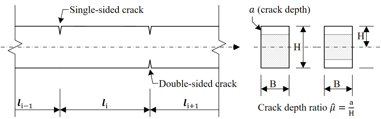
Figure 1. Crack parameters.

A crack is fully described by its position along the axis, and the crack depth ratio $\hat{\mu}$, as shown in Figure 1. According to the common practice in the field, see [7], a crack is modeled by a massless rotational spring. The spring flexibility $\theta=\theta(\hat{\mu})$ depends on the crack depth ratio $\hat{\mu}$, and on whether the crack is one-sided or two-sided, open or closed, and so on. The flexibility $\theta$ is equal to $0$ if there is no crack, and it increases with the crack depth. Explicit expressions for the functions $\theta(\hat{\mu})$ are provided in Section 3.

Remark 1.1.

The following discussion is applicable to both arches and beams, but to avoid repetitions we will refer just to arches.

Suppose that there are $m$ cracks along the length of the arch, located at $0<x_{1}<\dots<x_{m}<\pi$. For convenience, we denote $x_{0}=0$, and $x_{m+1}=\pi$. Consequently, the cracked arch is modeled as a collection of $m+1$ uniform arches over the intervals $l_{i}=(x_{i-1},x_{i}),\,i=1,\dots,m+1$, as shown in Figure 2(b).

We consider only the transverse motion of the arch, so its position can be described by the function $y=y(x,t)$, $0\leq x\leq\pi$, $t\geq 0$. The boundary conditions at the cracks enforce the continuity of the displacement field $y$, the bending moment $y^{\prime\prime}$, and the shear force $y^{\prime\prime\prime}$. Condition $y^{\prime}(x_{i}^{+},t)-y^{\prime}(x_{i}^{-},t)=\theta_{i}y^{\prime\prime}(x_{i}^{+},t)$ expresses the discontinuity of the arch slope at the $i$-th crack, where $\theta_{i}=\theta(\hat{\mu}_{i})$, see Figure 2(b).

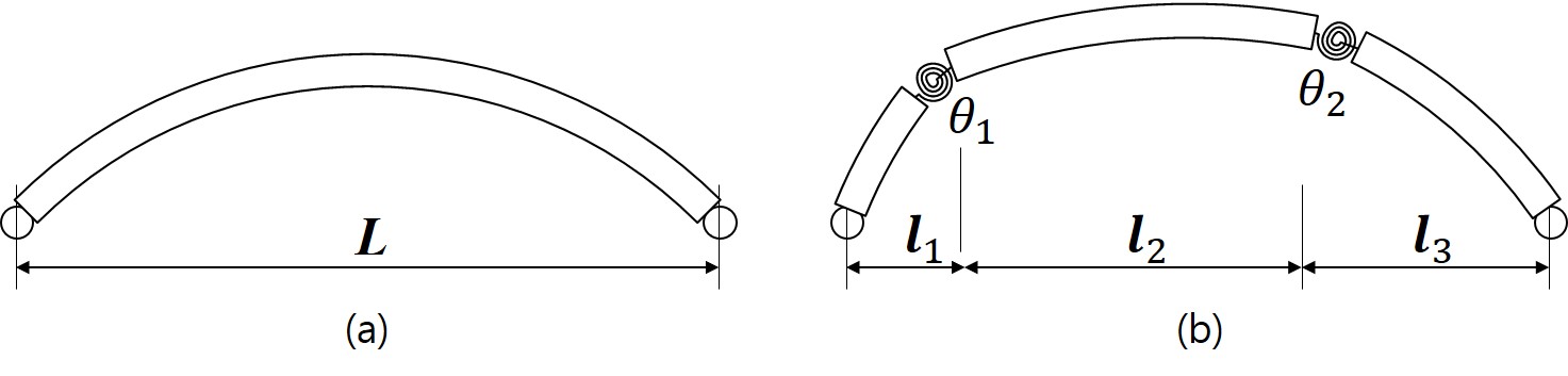
Figure 2. Beam or shallow arch: (a) uniform, (b) with two cracks.

To simplify the statement of the boundary conditions at the cracks, we introduce the notion of the jump $J[u](x)$ of a function $u=u(x)$ at any $x\in(0,\pi)$, as follows

(1.2) $$J[u](x)=u(x^{+})-u(x^{-}).$$

With this notation the conditions at the cracks (joint conditions) are

(1.3) $$J[y](x_{i},t)=0,\quad J[y^{\prime\prime}](x_{i},t)=0,\quad J[y^{\prime\prime\prime}](x_{i},t)=0,$$

and

(1.4) $$J[y^{\prime}](x_{i},t)=\theta_{i}y^{\prime\prime}(x_{i}^{+},t),$$

where $\theta_{i}=\theta(\hat{\mu}_{i})$, $i=1,2,\dots,m$ and $t\geq 0$. Note that $y^{\prime\prime}(x_{i}^{+},t)=y^{\prime\prime}(x_{i}^{-},t)$ by (1.3).

In Section 2 we review our recent results from [15] on the variational setting for cracked beams and arches. First, special Hilbert spaces $V,H_{0}^{1},H$ are defined satisfying

(1.5) $$V\subset H_{0}^{1}\subset H\subset(H_{0}^{1})^{\prime}\subset V^{\prime},$$

with continuous and dense embeddings. These spaces are broad enough to contain continuous functions with discontinuous derivatives at the joint points.

Then we introduce the operator $\mathcal{A}:V\to V^{\prime}$, by

(1.6) $$\langle\mathcal{A}u,v\rangle_{V}=\sum_{i=1}^{m+1}(u^{\prime\prime},v^{\prime\prime})_{i}+\sum_{i=1}^{m}\frac{1}{\theta}_{i}J[u^{\prime}](x_{i})J[v^{\prime}](x_{i}),$$

for any $u,v\in V$, where $J[u^{\prime}](x)=u^{\prime}(x^{+})-u^{\prime}(x^{-})$.

Our main result in [15] is that the solution $u$ of the equation $\mathcal{A}u=f$ in $H$ satisfies the joint conditions, including (1.4). Thus the operator $\mathcal{A}$ ”absorbs” the boundary conditions, as expected of the weak formulation of the steady state problem. This result allows us to mathematically justify the existence of the eigenvalues and the eigenfunctions of $\mathcal{A}$.

In Section 3 we consider relevant physical quantities, including the potential energy $U_{b}$, due to bending, and the potential energy $U_{a}$, due to the axial force. This is the only section in the paper, that contains physical variables. Their non-dimensional equivalents are used in all the other sections.

Typically, equations of motion are derived from the Hamilton’s Principle $\delta I=0$, which seeks the stationary paths of the action $I$. A closer examination of this statement in the framework of the Hilbert spaces reveals the importance of the subdifferential $\partial\phi$ of a convex lower-semicontinuous function $\phi$. The potential energies $U_{b}$, and $U_{a}$ are two examples of such functions.

Section 4 presents a brief review of these concepts. One can view the subdifferential, which can be multi-valued, as a generalization of the derivative. For example, let $\phi(x)=|x|,\,x\in{\mathbb{R}}$. Then $\partial\phi(x)=-1$, for $x<0$, $\partial\phi(x)=1$, for $x>0$, and $\partial\phi(0)=[-1,1]$. Geometrically, it means that the ”tangent” line to the graph of $\phi$ at $x=0$ can have any slope between $-1$ and $1$. We conclude Section 4 by deriving various expressions for the subdifferentials $\partial U_{b}$, and $\partial U_{a}$. In particular, we show that $\partial U_{b}=\mathcal{A}$.

Section 5 uses the Extended Hamilton’s Principle, which accommodates non-conservative forces, to derive the equations of motion. It contains our main result: the abstract equation of motion for cracked beams and arches is

(1.7) $$\ddot{y}+\partial U_{b}(y)+\partial U_{a}(y)+c_{d}\dot{y}=p,$$

where $\dot{y},\ddot{y}$ denote the time derivatives.

For beams, it is assumed that the influence of the axial force can be neglected. This case is considered in Section 6. The abstract equation for cracked beams is

(1.8) $$\ddot{y}+\mathcal{A}y+c_{d}\dot{y}=p.$$

If the beam contains no cracks, then (1.8) becomes $\ddot{y}+y^{\prime\prime\prime\prime}+c_{d}\dot{y}=p$, which is consistent with the classical Euler-Bernoulli theory.

Our main result in Section 7 is that the ”classical” equation for a cracked shallow arch is

$$\ddot{y}+y^{\prime\prime\prime\prime}$$

$$-\frac{1}{\pi}\left(\beta+\frac{1}{2}\int_{0}^{L}|y^{\prime}(x,t)|^{2}\,dx\right)\left(y^{\prime\prime}+\sum_{i=1}^{m}\theta_{i}y^{\prime\prime}(x_{i},t)\delta(x-x_{i})\right)+c_{d}\dot{y}=p,$$

where $\delta=\delta(x)$ is the delta function.

Motion in viscous media results in the additional term $\mu\mathcal{A}\dot{y}$, $\mu>0$ in the governing equations. Such a case is referred to as the strong damping motion. If the viscous effects are neglected ($\mu=0$), we have the weak damping case.

2. Variational setting for cracked beams and arches

This section contains a brief review of our results from [15], to which we refer for further details. Let $H$ be the Hilbert space

(2.1) $$H=\bigoplus_{i=1}^{m+1}L^{2}(l_{i}).$$

Let the inner product and the norm in $L^{2}(l_{i})$ be denoted by $(\cdot,\cdot)_{i}$ and $|\cdot|_{i}$ correspondingly. The inner product and the norm in $H$ are defined by

(2.2) $$(u,v)_{H}=\sum_{i=1}^{m+1}(u,v)_{i},\quad|u|^{2}_{H}=\sum_{i=1}^{m+1}|u|^{2}_{i}.$$

Consider the Sobolev space $H^{2}(a,b)$ on a bounded interval $(a,b)\subset{\mathbb{R}}$, and let $u\in H^{2}(a,b)$. Then $u,u^{\prime}$ are continuous functions on $[a,b]$, up to a set of measure zero, and $u^{\prime\prime}\in L^{2}(a,b)$. Therefore, for such $u$, we will always assume that $u,u^{\prime}\in C[a,b]$.

Define the linear space

(2.3) $$V=\left\{u\in\bigoplus_{i=1}^{m+1}H^{2}(l_{i})\,:\,u(0)=u(\pi)=0,\ J[u](x_{i})=0,\ i=1,\dots,m\right\}.$$

We interpret $u\in V$ as a continuous function on $[0,\pi]$, such that $u(0)=u(\pi)=0$, with $u^{\prime}\in L^{2}(0,\pi)$, i.e. $u\in H_{0}^{1}(0,\pi)$. Furthermore, $u|_{l_{i}}\in H^{2}(l_{i})$, and $u^{\prime}|_{l_{i}}\in C[x_{i-1},x_{i}]$ for $i=1,2,\dots,m+1$.

Define the inner product on $V$ by

(2.4) $$((u,v))_{V}=\sum_{i=1}^{m+1}(u^{\prime\prime},v^{\prime\prime})_{i}+\sum_{i=1}^{m}J[u^{\prime}](x_{i})J[v^{\prime}](x_{i}),\quad\text{for any}\ u,v\in V,$$

where $(u^{\prime\prime},v^{\prime\prime})_{i}=\int_{l_{i}}u^{\prime\prime}(x)v^{\prime\prime}(x)\,dx$.

The corresponding norm in $V$ is

(2.5) $$\|u\|_{V}^{2}=\sum_{i=1}^{m+1}|u^{\prime\prime}|^{2}_{i}+\sum_{i=1}^{m}|J[u^{\prime}](x_{i})|^{2},\quad\text{for any}\ u\in V,$$

where $|\cdot|_{i}$ is the norm in $L^{2}(l_{i})$. It can be shown that $V$ is a Hilbert space.

At this time we introduce the Hilbert space $H_{0}^{1}=H_{0}^{1}(0,\pi)$, with the inner product and the norm given by

(2.6) $$(u,v)_{1}=(u^{\prime},v^{\prime})_{H},\quad\|u\|_{1}^{2}=|u^{\prime}|_{H}^{2},\quad u,v\in H_{0}^{1}.$$

The norm in $(H_{0}^{1})^{\prime}$ will be denoted by $\|\cdot\|_{-1}$. It can be shown that the identity embedding $i:V\to H_{0}^{1}$ is linear, continuous, with a dense range in $H_{0}^{1}$. Furthermore, it is compact.

This allows us to define the Gelfand triple $V\subset H\subset V^{\prime}$, with the pairing $\langle\cdot,\cdot\rangle_{V}$ between $V$ and $V^{\prime}$ extending the inner product in $H$. This means that given $f\in H=H^{\prime}\subset V^{\prime}$, and $v\in V$, we have $\langle f,v\rangle_{V}=(f,v)_{H}$.

Also, we have

(2.7) $$V\subset H_{0}^{1}\subset H\subset\left(H_{0}^{1}\right)^{\prime}\subset V^{\prime},$$

with dense embeddings. Furthermore, the embeddings $V\subset H_{0}^{1}\subset H$ are compact.

Now we can introduce the operator $\mathcal{A}:V\to V^{\prime}$ that ”absorbs” the junction boundary conditions. This operator is central to the variational setting of problems for cracked beams and arches.

Definition 2.1.

Define the operator $\mathcal{A}$ on $V$ by

(2.8) $$\langle\mathcal{A}u,v\rangle_{V}=\sum_{i=1}^{m+1}(u^{\prime\prime},v^{\prime\prime})_{i}+\sum_{i=1}^{m}\frac{1}{\theta}_{i}J[u^{\prime}](x_{i})J[v^{\prime}](x_{i}),$$

for any $u,v\in V$. We will also write $\langle\mathcal{A}u,v\rangle$ for $\langle\mathcal{A}u,v\rangle_{V}$, if it does not cause a confusion.

Recall, that a linear operator $A:V\to V^{\prime}$ is called coercive, if there exists $c>0$, such that $\langle Au,u\rangle\geq c\|u\|^{2}_{V}$ for any $u\in V$. We have

Lemma 2.2.

Let $\mathcal{A}$ be defined by (2.8). Then $\mathcal{A}$ is a symmetric, continuous, linear, and coercive operator from $V$ onto $V^{\prime}$.

As was mentioned in Section 1, functions $u=u(x)$ modeling an arch with cracks are expected to satisfy certain boundary conditions. For convenience, we restate them here:

(2.9) $$u(0)=u(\pi)=0,\quad u^{\prime\prime}(0)=u^{\prime\prime}(\pi)=0,$$

and

(2.10) $$J[u](x_{i})=0,\quad J[u^{\prime\prime}](x_{i})=0,\quad J[u^{\prime\prime\prime}](x_{i})=0,\quad J[u^{\prime}](x_{i})=\theta_{i}u^{\prime\prime}(x_{i}^{+}),$$

for $i=1,\dots,m$.

The next theorem is the main result of this section.

Theorem 2.3.

Let the domain of $\mathcal{A}$ be $D(\mathcal{A})=\{v\in V:\mathcal{A}v\in H\}$.

1. If $u\in D(\mathcal{A})$, then $u|_{l_{i}}\in H^{4}(l_{i})$, $\mathcal{A}u=u^{\prime\prime\prime\prime}$ a.e. on $l_{i}$, $i=1,\dots,m+1$, and $u$ satisfies conditions (2.9)–(2.10).

2. Let $f\in H$, then equation $\mathcal{A}u=f$ in $V^{\prime}$ has a unique solution $u\in D(\mathcal{A})$.

Remark. The fact that $u^{\prime\prime\prime\prime}=f$ a.e. on $(0,\pi)$ in Theorem 2.3 does not imply that $u\in H^{4}(0,\pi)$. This is similar to the fact that the strong derivative $p^{\prime}$ of a step function $p$ on $(0,\pi)$ is zero a.e. on $(0,\pi)$. However, $p\not\in H^{1}(0,\pi)$.

Finally in this section we discuss the eigenvalues and the eigenfunctions of the operator $\mathcal{A}$. It was shown in Lemma 2.2 that $\mathcal{A}$ is a continuous, linear, symmetric, and coercive operator from $V$ onto $V^{\prime}$. Following [21, Section 2.2.1], $\mathcal{A}$ can also be considered as an unbounded operator in $H$.

Since the embedding $V\subset H$ is compact, the standard spectral theory for Sturm-Liouville boundary value problems is applicable. The eigenfunctions belong to $H$. Therefore, by Theorem 2.3, they are in the domain $D(\mathcal{A})\subset V$, thus continuous on $[0,\pi]$, and satisfy conditions (2.9)–(2.10).

We summarize these results in the following lemma.

Lemma 2.4.

Let $\mathcal{A}$ be the operator defined in (2.8). Then

1. There exists an increasing sequence of its real positive eigenvalues
   $\lambda^{4}_{1},\lambda^{4}_{2},\dots$, with $\lim_{k\to\infty}\lambda^{4}_{k}=\infty$.

2. The corresponding eigenfunctions $\varphi_{k}\in D(\mathcal{A})\subset V$, $k\geq 1$, and they satisfy the junction conditions (2.9)–(2.10).

3. The eigenfunctions $\varphi_{k}$ satisfy $\mathcal{A}\varphi_{k}=\lambda^{4}_{k}\varphi_{k}$ in $H$, $k\geq 1$. That is, $\varphi_{k}^{\prime\prime\prime\prime}(x)=\lambda^{4}_{k}\varphi_{k}(x)$ a.e. on every interval $l_{i}$, $i=1,\dots,m+1$.

4. The set $\{\varphi_{k}\}_{k=1}^{\infty}$ is a complete orthonormal basis in $H$.

An efficient method for a computational determination of the eigenvalues and the eigenfunctions of $\mathcal{A}$ (Modified Shifrin’s method) is discussed in [15].

3. Physical parameters and their non-dimensional equivalents

This is the only section in the paper that uses physical variables. All the other sections use their non-dimensional equivalents. Since both the physical variables and their equivalents use the same notation, such an arrangement helps to avoid confusing them. The physical variables are contained in Table 1 together with their units. Recall that the newton $N=kg\cdot m\cdot s^{-2}$ is the unit of force.

$L$	Length of bar	$m$
$T$	Final time	$s$
$y$	Bar deflection	$m$	$y=y(x,t)$
$p$	Transverse load/unit of length	$N\cdot m^{-1}$	$p=p(x,t)$
$c_{d}$	Damping coefficient	$kg\cdot m^{-1}s^{-1}$
$\kappa$	Bar curvature	$m^{-1}$
$\rho$	Volume mass density	$kg\cdot m^{-3}$
$E$	Young’s modulus	$N\cdot m^{-2}$
$A$	Cross-sectional area	$m^{2}$
$I$	Area moment of inertia	$m^{4}$
$r$	Radius of gyration	$m$	$r=\sqrt{I/A}$
$\omega_{0}$	$t$-scale	$s^{-1}$
$\omega$	Natural frequency	$s^{-1}$
$k$	Spring stiffness	$N\cdot m/rad$
$\theta$	Flexibility	$m$	$\theta=EI/k$
$T_{k}$	Kinetic energy	$J=N\cdot m$
$U_{a}$	Potential energy for axial force	$J$
$U_{b}$	Potential energy due to bending	$J$
$M$	Bending moment magnitude	$N\cdot m$
$S_{0}$	Initial tensile axial force	$N$
$S_{1}$	Tensile force due to deflection	$N$
$N$	Total axial force	$N$	$N=S_{0}+S_{1}$
$\mathcal{L}$	Lagrangian	$J$	$\mathcal{L}=T_{k}-U_{b}-U_{a}$
$\mathcal{W}_{ext}$	External work	$J$
$\mathcal{W}_{d}$	Dissipative work	$J$
$\mathcal{W}_{nc}$	Non-conservative work	$J$	$\mathcal{W}_{nc}=\mathcal{W}_{d}+\mathcal{W}_{ext}$
$e_{I}$	Energy normalization factor	$J$
$\beta$	Axial force renormalization	$1$
$\hat{\mu}$	Crack depth ratio	$1$
$\mu$	Normalized dynamic viscosity	$1$

Table 1. Nomenclature

To use the Extended Hamilton’s Principle we need to derive the Lagrangian $\mathcal{L}=T_{k}-U=T_{k}-U_{b}-U_{a}$, where $U_{b},U_{a}$ and $T_{k}$ are the potential and the kinetic energies. Also, we need the non-conservative external work $\mathcal{W}_{nc}$, which is the sum of the external work $\mathcal{W}_{ext}$ due to the load $p$, and the dissipative work $\mathcal{W}_{d}$ due to the damping force $\mathcal{F}_{d}$.

Let $y(x,t)$, $0\leq x\leq L$, be the position of the arch at the time $t\geq 0$. As usual, the dots denote the time derivatives, and the primes denote the spatial ones. For the kinetic energy we have

(3.1) $$T_{k}(y)=\frac{\rho A}{2}\int_{0}^{L}|\dot{y}(x,t)|^{2}\,dx.$$

The external work $\mathcal{W}_{ext}$ by the non-conservative load $p(x,t)$ is

(3.2) $$\mathcal{W}_{ext}(y)=\int_{0}^{L}p(x,t)y(x,t)\,dx.$$

The dissipative force $\mathcal{F}_{d}(x,t)=-c_{d}\dot{y}(x,t)$, $c_{d}\geq 0$ is a uniformly distributed viscous damping force acting only in the transverse direction. So, the dissipative work $\mathcal{W}_{d}$ done by the force is given by

(3.3) $$\mathcal{W}_{d}(y)=\int_{0}^{L}\mathcal{F}_{d}(x,t)y(x,t)\,dx=-c_{d}\int_{0}^{L}\dot{y}(x,t)y(x,t)\,dx.$$

The potential energy is

(3.4) $$U(y)=U_{b}(y)+U_{a}(y),$$

where $U_{b}$ is the potential energy due to the bending, and $U_{a}$ is the potential energy due to the axial force. The particular form of these terms depends on the presence of cracks and other factors.

To simplify the notations the $t$-dependency of $y$ is suppressed, if it does not cause a confusion.

Beam. Suppose that we have a uniform beam with no cracks, as shown in Figure 2(a). The magnitude $M(x)$ of the bending moment vector $\vec{M}(x)$ of the beam at any point $x\in(0,L)$ is given by $M(x)=EI\kappa(x)$, where $\kappa(x)$ is the curvature of the beam at $x$. Assuming $|y^{\prime}|\ll 1$, we get $\kappa(x)=y^{\prime\prime}(x)$, and $M(x)=EIy^{\prime\prime}(x)$. Accordingly, the bending potential energy of the beam is given by

(3.5) $$U_{b}(y)=\frac{EI}{2}\int_{0}^{L}(y^{\prime\prime})^{2}\,dx.$$

Now suppose that the beam has cracks as in Section 1, and in Figure 2(b). The cracks are at $0<x_{1}<\dots<x_{m}<L$. The standard approach to modeling a crack is to represent it as a massless rotational spring with the spring constant $k$, and the flexibility $\theta$.

The spring constant $k$ relates the torque ($N\cdot m$) to the angle of rotation. In our case this relationship takes the form $EIy^{\prime\prime}(x)=kJ[y^{\prime}](x)$, or $J[y^{\prime}](x)=\theta y^{\prime\prime}(x)$, where

(3.6) $$\theta=\frac{EI}{k}.$$

Thus the unit of the flexibility $\theta$ is $m$.

If the beam has a rectangular cross-section, as shown in Figure 1, then the area moment of inertia $I$ of the rectangle can be computed explicitly, and (3.6) can be simplified further. If the crack is double-sided, then by [19, Eq. (2.8)-(2.10)], the expression for the flexibility $\theta$ becomes

(3.7) $$\theta=6\pi H\hat{\mu}^{2}(0.535-0.929\hat{\mu}+3.500\hat{\mu}^{2}-3.181\hat{\mu}^{3}+5.793\hat{\mu}^{4}),$$

where $H$ is the half-height of the beam cross-section, and $\hat{\mu}=a/H$.

If the crack is single-sided, then by [19, Eq. (2.8)-(2.10)]

(3.8) $$\theta=6\pi H\hat{\mu}^{2}(0.6384-1.035\hat{\mu}+3.7201\hat{\mu}^{2}-5.1773\hat{\mu}^{3}+7.553\hat{\mu}^{4}-7.332\hat{\mu}^{5}),$$

where $H$ is the entire height of the beam cross-section, and $\hat{\mu}=a/H$.

The potential energy of the rotational spring with the spring constant $k$ is

$$U_{crack}=\frac{1}{2}k\alpha^{2},$$

where $\alpha$ is the angle of twist from its equilibrium position in radians. Since $J[y^{\prime}](x)\approx\alpha$ for small jumps in the slope of the beam, we conclude that the total bending potential energy of the cracked beam with $m$ cracks is

(3.9) $$U_{b}(y)=\frac{EI}{2}\int_{0}^{L}(y^{\prime\prime})^{2}\,dx+\frac{EI}{2}\sum_{i=1}^{m}\frac{1}{\theta_{i}}|J[y^{\prime}](x_{i})|^{2}.$$

Shallow arch. First, consider the uniform case. Following [22], the axial force $N$ in the uniform arch shown in Figure 2(a) is represented as the sum of two components $N=S_{0}+S_{1}$, where $S_{0}$ is the initial axial tensile force, and $S_{1}$ is the axial tensile force due to deflection. That is, the force is positive if it is tensile, and negative if it is compressing. The value of $S_{0}$ is assumed to be given, and the unknown force $S_{1}$ can be found through the deflection $y=y(x)$ as follows.

Let $\Delta L$ be the elongation of the arch due to the deflection. By the definition of the Young’s modulus $E$

(3.10) $$S_{1}=EA\frac{\Delta L}{L}.$$

The elongation is

(3.11) $$\Delta L =\int_{0}^{L}\sqrt{1+|y^{\prime}(x)|^{2}}\,dx-L$$

$$\approx\int_{0}^{L}\left(1+\frac{1}{2}|y^{\prime}(x)|^{2}\right)dx-L=\frac{1}{2}\int_{0}^{L}|y^{\prime}(x)|^{2}\,dx.$$

Then

(3.12) $$S_{1}=\frac{EA}{2L}\int_{0}^{L}|y^{\prime}(x)|^{2}\,dx.$$

The potential energy $U_{a}$ due to the axial force $N$ is

(3.13) $$U_{a}(y)=\frac{EA}{2L}(\Delta L^{*})^{2},$$

where $\Delta L^{*}=\frac{NL}{EA}$ is the elongation of the arch caused by the total axial force $N=S_{0}+S_{1}$. Therefore

(3.14) $$U_{a}(y)=\frac{L}{2EA}(S_{0}+S_{1})^{2}=\frac{L}{2EA}\left(S_{0}+\frac{EA}{2L}\int_{0}^{L}|y^{\prime}(x)|^{2}\,dx\right)^{2}.$$

Now suppose that the arch has cracks as in Section 1, and in Figure 2(b). To derive its axial potential energy $U_{a}(y)$, note that there exists a sequence of smooth functions $u_{n}$, such that $u_{n}\to y$ in $H^{1}_{0}(0,L)$, as $n\to\infty$. For such functions, the potential energy $U_{a}(u_{n})$ is given by the expression in (3.14), i.e.

(3.15) $$U_{a}(u_{n})=\frac{L}{2EA}\left(S_{0}+\frac{EA}{2L}\int_{0}^{L}|u_{n}^{\prime}(x)|^{2}\,dx\right)^{2},\quad n=1,2,\dots$$

Because of the continuity of this functional on $H^{1}_{0}(0,L)$, we conclude that we can pass to the limit in (3.15), as $n\to\infty$, to get

(3.16) $$U_{a}(y)=\frac{L}{2EA}\left(S_{0}+\frac{EA}{2L}\int_{0}^{L}|y^{\prime}(x)|^{2}\,dx\right)^{2},$$

i.e. the same expression as (3.14), even for an arch with cracks.

Non-dimensional variables. Now we find the non-dimensional equivalents for the above physical quantities. Define the $t$-scale $\omega_{0}$, and the radius of gyration $r$ by

(3.17) $$\omega_{0}=\left(\frac{\pi}{L}\right)^{2}\sqrt{\frac{EI}{\rho A}},\quad r=\sqrt{\frac{I}{A}}.$$

Then make the change of variables

(3.18) $$x\leftarrow\frac{\pi x}{L},\quad y\leftarrow\frac{y}{r},\quad p\leftarrow\frac{p}{EIr}\left(\frac{L}{\pi}\right)^{4},\quad t\leftarrow\omega_{0}t,\quad c_{d}\leftarrow\frac{c_{d}}{\rho A\omega_{0}}.$$

Temporarily distinguish the notation for the original physical variables by assigning them the $o$ subscript, and their non-dimensional equivalents by assigning them the $n$ subscript. For example, (3.18) transformation for $t$ says that $t_{n}=\omega_{0}t_{o}$. Then

(3.19) $$y_{o}(x_{o},t_{o})=ry_{n}(x_{n},t_{n})=ry_{n}\left(\frac{\pi x_{o}}{L},\omega_{0}t_{o}\right).$$

Therefore

(3.20) $$y_{o}^{\prime}(x_{o},t_{o})=r\frac{\pi}{L}y_{n}^{\prime}(x_{n},t_{n}),\quad y_{o}^{\prime\prime}(x_{o},t_{o})=r\left(\frac{\pi}{L}\right)^{2}y_{n}^{\prime\prime}(x_{n},t_{n}),$$

and

(3.21) $$\dot{y}_{o}(x_{o},t_{o})=r\omega_{0}\dot{y}_{n}(x_{n},t_{n}),\quad\ddot{y}_{o}(x_{o},t_{o})=r\omega_{0}^{2}\ddot{y}_{n}(x_{n},t_{n}).$$

Let the energy normalization factor $e_{I}$ be defined by

(3.22) $$e_{I}=\frac{L}{\pi}\rho Ar^{2}\omega_{0}^{2}=\frac{L}{\pi}\rho I\omega_{0}^{2}=\left(\frac{\pi}{L}\right)^{3}r^{2}EI.$$

Then the kinetic energy $T_{k,o}$ from (3.1) is transformed according to

(3.23) $$T_{k,o}(y_{o}) =\frac{\rho A}{2}\int_{0}^{L}|\dot{y}_{o}(x_{o},t_{o})|^{2}\,dx_{o}=\frac{L}{\pi}\rho Ar^{2}\omega_{0}^{2}\frac{1}{2}\int_{0}^{\pi}|\dot{y}_{n}(x_{n},t_{n})|^{2}\,dx_{n}$$

$$=e_{I}\frac{1}{2}|\dot{y}_{n}|_{H}^{2}=e_{I}T_{k,n}(y_{n}).$$

Consistent with the definition of the flexibility $\theta$ in (3.6), we use the transformation $\theta\leftarrow\pi\theta/L$. Therefore, for the bending potential energy (3.9) we have

(3.24) $$U_{b,o}(y_{o})=\frac{EI}{2}\int_{0}^{L}|y^{\prime\prime}_{o}(x_{o})|^{2}\,dx_{o}+\frac{EI}{2}\sum_{i=1}^{m}\frac{1}{\theta_{i,o}}|J[y^{\prime}_{o}](x_{i,o})|^{2}$$

$$=\left(\frac{\pi}{L}\right)^{3}r^{2}EI\left[\frac{1}{2}\int_{0}^{\pi}|y^{\prime\prime}_{n}(x_{n})|^{2}\,dx_{n}+\frac{1}{2}\sum_{i=1}^{m}\frac{1}{\theta_{i,n}}|J[y^{\prime}_{n}](x_{i,n})|^{2}\right]$$

$$=e_{I}U_{b,n}(y_{n}).$$

The potential energy $U_{a}$ due to the axial force is given by (3.16). After the substitution (3.18) we get

$$U_{a,o}(y_{o})=\frac{L}{2EA}\left(S_{0}+\frac{EA}{2L}r^{2}\frac{\pi}{L}\int_{0}^{\pi}|y^{\prime}_{n}(x_{n})|^{2}\,dx_{n}\right)^{2}$$

$$=\frac{L}{2EA}\frac{(EA)^{2}\pi^{2}r^{2}r^{2}}{L^{4}}\left(\frac{L^{2}S_{0}}{EA\pi r^{2}}+\frac{1}{2}\int_{0}^{\pi}|y^{\prime}_{n}(x_{n})|^{2}\,dx_{n}\right)^{2}$$

$$=\frac{e_{I}}{2\pi}\left(\beta+\frac{1}{2}\int_{0}^{\pi}|y^{\prime}_{n}(x_{n})|^{2}\,dx_{n}\right)^{2},$$

where the non-dimensional $\beta\in{\mathbb{R}}$ is a renormalization of the axial force $S_{0}$.

Similarly, we conclude that $\mathcal{W}_{ext}$, and $\mathcal{W}_{d}$ are transformed by (3.18) into their non-dimensional equivalents in the same way:

(3.25) $$T_{k}\leftarrow\frac{T_{k}}{e_{I}},\quad U_{a}\leftarrow\frac{U_{a}}{e_{I}},\quad U_{b}\leftarrow\frac{U_{b}}{e_{I}},\quad\mathcal{W}_{ext}\leftarrow\frac{\mathcal{W}_{ext}}{e_{I}},\quad\mathcal{W}_{d}\leftarrow\frac{\mathcal{W}_{d}}{e_{I}}.$$

Therefore, the expressions for the non-dimensional quantities are

(3.26) $$T_{k}(y)=\frac{1}{2}|\dot{y}|^{2}_{H},\quad\mathcal{W}_{ext}(y)=(p,y)_{H},\quad\mathcal{W}_{d}(y)=-c_{d}(\dot{y},y)_{H},$$

(3.27) $$U_{b}(y)=\frac{1}{2}\left(|y^{\prime\prime}|^{2}_{H}+\sum_{i=1}^{m}\frac{1}{\theta}_{i}|J[y^{\prime}](x_{i})|^{2}\right),$$

(3.28) $$U_{a}(y)=\frac{1}{2\pi}\left(\beta+\frac{1}{2}|y^{\prime}|^{2}_{H}\right)^{2},$$

where $\beta\in{\mathbb{R}}$.

Natural beam frequencies. Equation of harmonic transverse oscillations $v=v(x)$ of a uniform beam defined on interval $(0,L)$ is

(3.29) $$EIv^{\prime\prime\prime\prime}(x)=\omega^{2}\rho Av(x),\quad 0<x<L.$$

For a cracked beam, equation (3.29) is satisfied on every subinterval $(x_{i-1},x_{i})$, $i=1,\dots,m+1$.

Using the transformations to the non-dimensional variables (3.17)–(3.21), we get

$$EIr\left(\frac{\pi}{L}\right)^{4}v_{n}^{\prime\prime\prime\prime}(x_{n},t_{n})=\omega^{2}\rho Arv_{n}(x_{n},t_{n}),$$

where $v_{n}(x_{n},t_{n})$ is $v(x,t)$ in the new (non-dimensional) variables. Dropping the subscript $n$, we obtain the equation for $v$ in the non-dimensional quotients

$$v^{\prime\prime\prime\prime}=\omega^{2}\left(\frac{L}{\pi}\right)^{4}\frac{\rho A}{EI}v.$$

Comparing this equation with the definition of the eigenvalues and the eigenfunctions $\varphi_{k}^{\prime\prime\prime\prime}=\lambda_{k}^{4}\varphi_{k}$, we conclude that the natural beam frequencies are given by

(3.30) $$\omega_{k}=\lambda_{k}^{2}\left(\frac{\pi}{L}\right)^{2}\sqrt{\frac{EI}{\rho A}},\quad k\geq 1.$$

4. Convex functions and subdifferentials

Subdifferentials provide the proper mathematical framework for the abstract formulation of equations of motion. Following [3, Section 1.2], let $X$ be a Hilbert space. A function $\phi:X\to(-\infty,+\infty]$ is called proper and convex on $X$, if $\phi$ is not identically $+\infty$, and

(4.1) $$\phi((1-\lambda)x+\lambda y)\leq(1-\lambda)\phi(x)+\lambda\phi(y),$$

for any $x,y\in X$, and $\lambda\in[0,1]$. The function $\phi$ is called lower-semicontinuous on $X$, if every level set $\{x\in X:\phi(x)\leq c\},\,c>-\infty$, is closed in $X$.

Given a proper, convex, lower-semicontinuous function $\phi$ on $X$, the subdifferential $\partial\phi:X\to X^{\prime}$ is defined by

(4.2) $$\partial\phi(x)=\{x^{*}\in X^{\prime}\ :\ \phi(y)\geq\phi(x)+\langle x^{*},y-x\rangle\},$$

for any $y\in X$. Thus $\partial\phi\subset X\times X^{\prime}$.

In general, $\partial\phi$ does not have to be defined everywhere on $X$. Furthermore, the mapping $x\to\partial\phi(x)\subset X^{\prime}$ can be multi-valued. Geometrically, if $\partial\phi(x)$ is single-valued at $x\in X$, then $y\to\phi(x)+\langle\partial\phi(x),y-x\rangle$ is the tangent plane to the graph of $\phi$ at $x$.

Let $D(\phi)=\{x\in X:\phi(x)<\infty\}$, and $D(\partial\phi)=\{x\in X:\partial\phi(x)\not=\emptyset\}$. Note that if $x\in D(\partial\phi)$, then $x\in D(\phi)$. Indeed, $\phi$ is a proper function. Therefore $D(\phi)\not=\emptyset$. Choose $y\in D(\phi)$, and $x^{*}\in\partial\phi(x)$. Then $\phi(x)\leq\phi(y)-\langle x^{*},y-x\rangle<\infty$, as claimed.

Let $f:X\to{\mathbb{R}}$. The directional derivative $f^{\prime}(x;y)$ of $f$ at $x\in X$ in the direction $y\in X$ is defined by

(4.3) $$f^{\prime}(x;y)=\lim_{\alpha\to 0+}\frac{f(x+\alpha y)-f(x)}{\alpha}.$$

A function $f$ is said to be Gâteaux differentiable at $x\in X$, if there exists $(\nabla f)(x)\in X^{\prime}$, such that

(4.4) $$f^{\prime}(x;y)=\langle\nabla f(x),y\rangle,$$

for any $y\in X$. The linear functional $(\nabla f)(x)$ is called the Gâteaux derivative of $f$ at $x\in X$.

If the convergence in (4.3) is uniform in $y$ on bounded subsets, then $f$ is said to be Fréchet differentiable.

The Gâteaux differentiability of $f$ is a more restrictive condition, than $f$ is having a subdifferential. The following lemma is proved in [3, Section 1.2]:

Lemma 4.1.

If $\phi$ is convex and Gâteaux differentiable at $x\in X$, then $\partial\phi(x)=\nabla\phi(x)$, and $\partial\phi(x)$ is a singleton.

Recall that an operator $A:X\to X^{\prime}$ is called symmetric, if $\langle Au,v\rangle=\langle Av,u\rangle$, for any $u,v\in D(A)$.

Theorem 4.2.

Let $X$ be a Hilbert space, and $A:X\to X^{\prime}$ be a linear, continuous, and symmetric operator, such that $D(A)=X$, and $\langle Au,u\rangle\geq 0$ for any $u\in X$. Then function $\phi:X\to{\mathbb{R}}$ defined by

(4.5) $$\phi(u)=\frac{1}{2}\langle Au,u\rangle,\quad u\in X,$$

is convex, proper, and lower-semicontinuous on $X$. Moreover, it is Fréchet differentiable on $X$ with $\nabla\phi(u)=\partial\phi(u)=Au$ for any $u\in X$, and $D(\phi)=D(\partial\phi)=X$.

Proof.

To see that $\varphi$ is convex, let $0\leq\lambda\leq 1$, and $u,v\in X$. Then

$$\phi(\lambda u+(1-\lambda)v)=\frac{1}{2}\left[\lambda^{2}\langle Au,u\rangle+2\lambda(1-\lambda)\langle Au,v\rangle+(1-\lambda)^{2}\langle Av,v\rangle\right]$$

$$=\frac{1}{2}\left[\lambda\langle Au,u\rangle+(1-\lambda)\langle Av,v\rangle-\lambda(1-\lambda)\langle A(u-v),(u-v)\rangle\right]$$

$$\leq\lambda\phi(u)+(1-\lambda)\phi(v).$$

Since $A$ is continuous, function $\phi$ is continuous on $X$. In particular, it is lower-semicontinuous on $X$. From the continuity of $A$, we have $\|Av\|_{X^{\prime}}\leq C\|v\|_{X}$, for some $C>0$. Since

$$\phi(v)-\phi(u)-\langle Au,v-u\rangle=\frac{1}{2}\langle A(v-u),v-u\rangle,$$

we conclude that

(4.6) $$|\phi(v)-\phi(u)-\langle Au,v-u\rangle|\leq\frac{C}{2}\|v-u\|_{X}^{2}.$$

Therefore $Au=(\nabla\phi)(u)$ is the Gâteaux (even Fréchet) derivative of $\phi$ at $u\in X$, and $\partial\phi=A$ is its single-valued subdifferential, with $D(\partial\phi)=D(\varphi)=X$. ∎

Example 4.3.

Let $V$ be the Hilbert space defined in (2.3), and $\mathcal{A}$ be the linear operator defined in (2.8). Let

(4.7) $$\varphi(u)=\frac{1}{2}\langle\mathcal{A}u,u\rangle,\quad u\in V.$$

By Theorem 4.2 with $X=V$, function $\varphi:V\to{\mathbb{R}}$ is proper, convex, and lower-semicontinuos on $V$. Furthermore, $D(\partial\varphi)=V$, and $\partial\varphi(u)=\mathcal{A}u$, for any $u\in V$.

For a general $u\in V$, the expression for $\partial\varphi(u)\in V^{\prime}$ is complicated. However, if we assume that $u$ is somewhat more regular, then we can get a simpler expression for it.

Suppose that $u\in D(\mathcal{A})\subset V$. Then, by Theorem 2.3, we have $\mathcal{A}u=u^{\prime\prime\prime\prime}$ a.e. on every interval $l_{i}$, $i=1,\dots,m+1$. Thus, we can say that $\partial\varphi(u)=u^{\prime\prime\prime\prime}$ a.e. on every such interval.

Suppose further, that $u\in H_{0}^{1}(0,\pi)\cap H^{4}(0,\pi)\subset D(\mathcal{A})$. Then $u^{\prime\prime\prime\prime}\in L^{2}(0,\pi)$, and $u^{\prime}$ is smooth. Thus $J[u^{\prime}](x_{i})=0$ for any $i=1,\dots,m$, and we have

(4.8) $$\langle\partial\varphi(u),v\rangle=\langle\mathcal{A}u,v\rangle=\int_{0}^{\pi}u^{\prime\prime}(x)v^{\prime\prime}(x)\,dx=\int_{0}^{\pi}u^{\prime\prime\prime\prime}(x)v(x)\,dx,$$

for any $v\in V$. Therefore, in this case $\partial\varphi(u)=u^{\prime\prime\prime\prime}$ a.e. on $[0,\pi]$.

Example 4.4.

Let $H_{0}^{1}=H_{0}^{1}(0,\pi)$ be the Hilbert space defined in (2.6), and $\langle\cdot,\cdot\rangle_{1}$ be the duality pairing between $H_{0}^{1}$ and $(H_{0}^{1})^{\prime}$. Let $\mathcal{B}$ be the linear operator defined by

(4.9) $$\langle\mathcal{B}u,v\rangle_{1}=(u^{\prime},v^{\prime})_{H},\quad u,v\in H_{0}^{1}.$$

Then $\mathcal{B}:H_{0}^{1}\to(H_{0}^{1})^{\prime}$ is continuous, symmetric and coercive on $H_{0}^{1}$. In particular, $\mathcal{B}$ is positive, and its range is $(H_{0}^{1})^{\prime}$.

Let

(4.10) $$\psi(u)=\frac{1}{2}\langle\mathcal{B}u,u\rangle,\quad u\in H_{0}^{1}.$$

Theorem 4.2 is applicable with $X=H_{0}^{1}$, and $A=\mathcal{B}$. We conclude that the function $\psi:H_{0}^{1}\to{\mathbb{R}}$ is proper, convex, and lower-semicontinuos on $H_{0}^{1}$. Furthermore, $D(\partial\psi)=H_{0}^{1}$, and $\partial\psi(u)=\mathcal{B}u\in(H_{0}^{1})^{\prime}$, for any $u\in H_{0}^{1}$.

As in Example 4.3, a simpler expression for the subdifferential $\partial\psi(u)$ can be obtained assuming an additional regularity of $u\in H_{0}^{1}$.

Suppose that $u\in V\subset H_{0}^{1}$. Then we have

(4.11) $$\langle\mathcal{B}u,v\rangle_{1} =(u^{\prime},v^{\prime})_{H}=\int_{0}^{\pi}u^{\prime}(x)v^{\prime}(x)\,dx=$$

$$-\sum_{i=1}^{m}J[u^{\prime}(x_{i})]v(x_{i})-\sum_{i=1}^{m+1}(u^{\prime\prime},v)_{i},$$

for any $v\in H_{0}^{1}$. Therefore, in this case,

(4.12) $$\partial\psi(u)=\mathcal{B}u=-\sum_{i=1}^{m}J[u^{\prime}](x_{i})\delta(x-x_{i})-u^{\prime\prime},$$

where $\delta(x-a),\,a\in[0,\pi]$ is the element of $(H_{0}^{1})^{\prime}$, defined by $\langle\delta(x-a),v\rangle_{1}=v(a)$, for any $v\in H_{0}^{1}$.

Suppose further, that $u\in D(\mathcal{A})\subset V$. Then, by Theorem 2.3, $u$ satisfies conditions (2.9)–(2.10). In particular, $J[u^{\prime}](x_{i})=\theta_{i}u^{\prime\prime}(x_{i})$. Thus, with this additional assumption on $u$, we have

(4.13) $$\partial\psi(u)=\mathcal{B}u=-\sum_{i=1}^{m}\theta_{i}u^{\prime\prime}(x_{i})\delta(x-x_{i})-u^{\prime\prime},$$

which is still an element of $(H_{0}^{1})^{\prime}$.

5. Extended Hamilton’s principle

To derive the governing equations for beams and arches, we use the Extended Hamilton’s Principle, which accommodates non-conservative forces, see [17].

The Principle states that the motion $y=y(x,t)$ of the system gives a stationary value to the action of the system, i.e. to the integral

(5.1) $$I(y)=\int_{t_{1}}^{t_{2}}(\mathcal{L}+\mathcal{W}_{nc})\,dt,$$

where the Lagrangian $\mathcal{L}=T_{k}-U$ is the difference between the kinetic energy $T_{k}$ and the potential energy $U=U_{b}+U_{a}$. The term $\mathcal{W}_{nc}=\mathcal{W}_{d}+\mathcal{W}_{ext}$ for the non-conservative external work $\mathcal{W}_{nc}$ is the sum of the external work $\mathcal{W}_{ext}$, due to the load $p$, and the dissipative work $\mathcal{W}_{d}$, due to a damping force $\mathcal{F}_{d}$.

Thus (5.1) becomes

(5.2) $$I(y)=\int_{t_{1}}^{t_{2}}\left(T_{k}(y)-U_{b}(y)-U_{a}(y)+\mathcal{W}_{d}(y,\dot{y})+\mathcal{W}_{ext}(y)\right)\,dt,$$

where the components of the action are given in (3.26)–(3.28).

The traditional way of expressing the fact that the motion of the system gives a stationary value to the functional $I$ defined in (5.2), is to say that its variation $\delta I=0$. Let us examine this statement in more detail within the framework of the Hilbert spaces.

Recall that the Hilbert spaces $V,H_{0}^{1}$, and $H$ were defined in Section 2. Define

$$W=\{y\ :\ y\in L^{2}(0,T;V),\ \dot{y}\in L^{2}(0,T;H),\ \ddot{y}\in L^{2}(0,T;V^{\prime})\},$$

where the derivatives are taken in the sense of distributions, [21, Chapter 2]. This is a Hilbert space with the standard inner product and the norm.

Given $\eta\in W$, the directional derivative $I^{\prime}(y,\eta)$ is defined by

(5.3) $$I^{\prime}(y,\eta)=\lim_{\alpha\to 0+}\frac{I(y+\alpha\eta)-I(y)}{\alpha},$$

which is consistent with (4.3).

The Gâteaux derivative $\nabla I(y)$ (if exists) is an element of the dual $W^{\prime}$, such that

(5.4) $$I^{\prime}(y,\eta)=\langle\nabla I(y),\eta\rangle_{W},$$

for any $\eta\in W$, see Section 4, and [3, Section 1.2].

Functional $I$ has a stationary value at $y$ means that $\nabla I(y)=0$, which gives the meaning to the infinitesimal variation equation $\delta I=0$.

To derive the governing equation, one has to transform the stationary value equation $\nabla I(y)=0$ into a more explicit form by computing the directional derivatives of $I$ along the specially chosen $\eta\in W$.

Let $\eta(x,t)=\zeta(t)v(x)$, where $\zeta:[t_{1},t_{2}]\to{\mathbb{R}}$ is a smooth function satisfying $\zeta(t_{1})=\zeta(t_{2})=0$, and $v\in V$.

To obtain $\nabla I(y)$, we compute the corresponding directional derivatives for every term in (5.2) for the same $\eta=\zeta v$. First, notice that

(5.5) $$T_{k}(y+\alpha\eta)-T_{k}(y)=\alpha(\dot{y},v)_{H}\dot{\zeta}+\frac{\alpha^{2}}{2}|\dot{\zeta}|^{2}\,|v|_{H}^{2}.$$

By the definition of the directional derivative, $T_{k}^{\prime}(y,\eta)=\int_{t_{1}}^{t_{2}}(\dot{y},v)_{H}\dot{\zeta}\,dt$. Integrating by parts in $t$, and using $\zeta(t_{1})=\zeta(t_{2})=0$, we get

(5.6) $$T_{k}^{\prime}(y,\eta)=\int_{t_{1}}^{t_{2}}(\dot{y}(t),v)_{H}\dot{\zeta}(t)\,dt=-\int_{t_{1}}^{t_{2}}\langle\ddot{y}(t),v\rangle_{V}\zeta(t)\,dt.$$

Similarly,

(5.7) $$\mathcal{W}_{ext}^{\prime}(y,\eta)=\int_{t_{1}}^{t_{2}}(p(t),v)_{H}\zeta(t)\,dt,$$

where the dependency of $p=p(x,t)$ on $x$ is suppressed.

The work $\mathcal{W}_{d}$ done by the non-conservative force $\mathcal{F}_{d}$ is not covered by the classical Hamilton’s Principle. To accommodate such a case, the Principle is extended by introducing the Rayleigh’s dissipation functional, for which the action is defined in a non-variational manner, see [17] for details. In our case it implies that

(5.8) $$\mathcal{W}_{d}^{\prime}(y,\eta)=-c_{d}\int_{t_{1}}^{t_{2}}(\dot{y}(t),v)_{H}\zeta(t)\,dt.$$

The expressions for the potential energies $U_{b}$ and $U_{a}$ depend on whether the system is a beam or an arch, and on the presence of cracks. They are given in (3.27)–(3.28). In every case, $U_{b}(u)$ is a convex, lower-semicontinuous function on $V$, and $U_{a}(u)$ is a convex, lower-semicontinuous function on $H_{0}^{1}$. Therefore they admit subdifferentials $\partial U_{b}$ and $\partial U_{a}$, on $V$ and $H_{0}^{1}$ correspondingly, see Section 4.

If $U_{b}$ and $U_{a}$ are Gateaux differentiable, then the subdifferentials are equal to their Gateaux derivatives. Thus, we have for $\eta=\zeta v$

(5.9) $$U_{b}^{\prime}(y,\eta) =\int_{t_{1}}^{t_{2}}\langle\partial U_{b}(y(t)),v\rangle_{V}\zeta(t)\,dt,$$

(5.10) $$U_{a}^{\prime}(y,\eta) =\int_{t_{1}}^{t_{2}}\langle\partial U_{a}(y(t)),v\rangle_{1}\zeta(t)\,dt.$$

The stationary value equation $\nabla I(y)=0$, for $I(y)$ given by (5.2), implies

(5.11) $$0=(\nabla I(y),\eta)_{W}=I^{\prime}(y,\eta)\\ =\int_{t_{1}}^{t_{2}}\left[(-c_{d}\dot{y}+p(t),v)_{H}-\langle\ddot{y}+\partial U_{b}(y(t)),v\rangle_{V}-\langle\partial U_{a}(y(t)),v\rangle_{1}\right]\zeta(t)\,dt.$$

Since $\zeta$ is an arbitrary smooth function on $[t_{1},t_{2}]$, we get

$$(-c_{d}\dot{y}+p(t),v)_{H}-\langle\ddot{y}+\partial U_{b}(y(t)),v\rangle_{V}-\langle\partial U_{a}(y(t)),v\rangle_{1}=0,$$

for any $v\in V$, and almost any $t\in[0,T]$. This can further be written as

(5.12) $$\langle-\ddot{y}-\partial U_{b}(y(t))-\partial U_{a}(y(t))-c_{d}\dot{y}+p(t),v\rangle_{V}=0.$$

Thus (5.12) implies the following main result: equation

(5.13) $$\ddot{y}+\partial U_{b}(y)+\partial U_{a}(y)+c_{d}\dot{y}=p,$$

is the abstract governing equation of the system in $V^{\prime}$, a.e. for $t\in[0,T]$. Note: $\partial U_{b}:V\to V^{\prime}$, and $\partial U_{a}:H_{0}^{1}\to(H_{0}^{1})^{\prime}$.

6. Beam equation

Uniform beam. Suppose that we have a uniform beam with no cracks, as shown in Figure 2(a). The classical Euler-Bernoulli beam theory [16] assumes that the beam motion is due mainly to its bending, while the influence of the axial force is negligible. Thus we let $U_{a}=0$.

By (3.27) the bending potential energy of the uniform beam is given by

(6.1) $$U_{b}(y)=\frac{1}{2}|y^{\prime\prime}|^{2}_{H}.$$

Define operator $\mathcal{A}:V\to V^{\prime}$ by

(6.2) $$\langle\mathcal{A}u,v\rangle=(u^{\prime\prime},v^{\prime\prime})_{H},$$

for any $u,v\in V$. The operator $\mathcal{A}$ is linear, symmetric, and coercive on $V$. Then

(6.3) $$U_{b}(u)=\frac{1}{2}\langle\mathcal{A}u,u\rangle,$$

for any $u\in V$. By Theorem 4.2, $U_{b}$ is a convex, lower-semicontinuous function on $V$. Furthermore, $\partial U_{b}(u)=\mathcal{A}u$. From (5.13), the abstract Uniform Beam equation in $V^{\prime}$ is

(6.4) $$\ddot{y}+\mathcal{A}y+c_{d}\dot{y}=p.$$

Assume that $u\in D(\mathcal{A})$. By Example 4.3, $\mathcal{A}u=u^{\prime\prime\prime\prime}$ for such $u$. Therefore, with this assumption, equation (6.4) can be written as

(6.5) $$\ddot{y}+y^{\prime\prime\prime\prime}+c_{d}\dot{y}=p,$$

which is the classical Euler-Bernoulli form of the Beam equation for beams without cracks. To obtain this equation in physical variables, reverse the substitutions in Section 3.

Beam with cracks. Now suppose that the beam has cracks as in Section 1, and in Figure 2(b). Continuing with the classical Euler-Bernoulli beam theory we disregard the axial force, and let $U_{a}=0$.

By (3.27), the bending potential energy of the cracked beam with $m$ cracks is

(6.6) $$U_{b}(y)=\frac{1}{2}\left(|y^{\prime\prime}|^{2}_{H}+\sum_{i=1}^{m}\frac{1}{\theta}_{i}|J[y^{\prime}](x_{i})|^{2}\right).$$

Arguing as in Example 4.3, we get that $U_{b}$ is a convex, lower-semicontinuous function on $V$.

Define operator $\mathcal{A}:V\to V^{\prime}$ as in equation (2.8), i.e.

(6.7) $$\langle\mathcal{A}u,v\rangle=\sum_{i=1}^{m+1}(u^{\prime\prime},v^{\prime\prime})_{i}+\sum_{i=1}^{m}\frac{1}{\theta}_{i}J[u^{\prime}](x_{i})J[v^{\prime}](x_{i}),$$

for any $u,v\in V$. By Lemma 2.2, the operator $\mathcal{A}$ is linear, symmetric, and coercive on $V$. Then

(6.8) $$U_{b}(u)=\frac{1}{2}\langle\mathcal{A}u,u\rangle,$$

for any $u\in V$.

By Theorem 4.2, $\partial U_{b}(u)=\mathcal{A}u$. Therefore the abstract equation for the beam with cracks is

(6.9) $$\ddot{y}+\mathcal{A}y+c_{d}\dot{y}=p,$$

which is satisfied in $V^{\prime}$, a.e. for $t\in[0,T]$.

Furthermore, using Example 4.3, if $u\in D(\mathcal{A})$, then $u$ satisfies the boundary conditions of the problem, i.e. (2.9) and (2.10), as well as $\mathcal{A}u=u^{\prime\prime\prime\prime}$ a.e. on every interval $l_{i}$, $i=1,\dots,m+1$.

Then equation (6.9) can be written as

(6.10) $$\ddot{y}+y^{\prime\prime\prime\prime}+c_{d}\dot{y}=p.$$

We can call it the classical Beam equation for beams with cracks. While this equation looks the same as the Beam equation for beams with no cracks (6.5), its abstract formulation (6.9) uses the operator $\mathcal{A}$ defined by (6.7), rather than by (6.2). In particular, $y(\cdot,t)\in V$, a.e. $t\in[0,T]$.

Strong damping. Viscous effects on the beam and arch motion are discussed in [2, 11]. Considerations based on the Voigt model for viscoelasticity result in the additional term $\mu\mathcal{A}\dot{y}$ in the governing equations. Here $\mu>0$ is a non-dimensional normalized dynamic viscosity coefficient.

If such a term is present, we refer to the model as having the strong damping. Otherwise, if $\mu=0$, the model is for the weak damping. In particular, equations (6.9) and (6.10) describe the weak beam damping motion case. The corresponding non-dimensional abstract and classical equations in the presence of the strong damping $\mu>0$ are

(6.11) $$\ddot{y}+\mathcal{A}y+\mu\mathcal{A}\dot{y}+c_{d}\dot{y}=p,$$

and

(6.12) $$\ddot{y}+y^{\prime\prime\prime\prime}+\mu\dot{y}^{\prime\prime\prime\prime}+c_{d}\dot{y}=p.$$

7. Arch equation

Uniform shallow arch. The potential energy for the arch contains the term $U_{a}$, due to the axial force. By (3.28)

(7.1) $$U_{a}(y)=\frac{1}{2\pi}\left(\beta+\frac{1}{2}|y^{\prime}|^{2}_{H}\right)^{2}.$$

To compute the subdifferential of $U_{a}$, note that for $u\in V$,

(7.2) $$\partial U_{a}(u)=\frac{1}{\pi}\left(\beta+\frac{1}{2}|y^{\prime}|^{2}_{H}\right)\partial\psi(u),$$

where $\psi$ is

(7.3) $$\psi(u)=\frac{1}{2}|u^{\prime}|^{2}_{H}=\frac{1}{2}\langle\mathcal{B}u,u\rangle,\quad u\in V,$$

see Example 4.4. Since there are no cracks in the arch, we have $\partial\psi(u)=-u^{\prime\prime}$, per (4.12).

Using the subdifferential $\partial U_{b}(u)=\mathcal{A}u$, for $\mathcal{A}$ defined by (6.2), the abstract form of the uniform shallow arch equation is

(7.4) $$\ddot{y}+\mathcal{A}y-\frac{1}{\pi}\left(\beta+\frac{1}{2}|y^{\prime}|^{2}_{H}\right)y^{\prime\prime}+c_{d}\dot{y}=p,$$

in $V^{\prime}$, a.e. on $[0,T]$.

Its classical form is

(7.5) $$\ddot{y}+y^{\prime\prime\prime\prime}-\frac{1}{\pi}\left(\beta+\frac{1}{2}\int_{0}^{\pi}|y^{\prime}(x,t)|^{2}\,dx\right)y^{\prime\prime}+c_{d}\dot{y}=p,$$

cf. [22, eq. (6)].

Arch with cracks. Now suppose that the arch has cracks as in Section 1, and in Figure 2(b). Its axial potential energy $U_{a}(y)$ has the same expression as (7.1), even if the arch has cracks.

However, the subdifferential $\partial U_{a}(u)$ is different from the one in the smooth case. It has been computed in Example 4.4 as

(7.6) $$\partial\psi(u)=\mathcal{B}u=-\sum_{i=1}^{m}J[u^{\prime}](x_{i})\delta(x-x_{i})-u^{\prime\prime},$$

for $u\in V$. The bending potential $U_{b}$ is given by (6.6). Then its subdifferential $\partial U_{b}(u)=\mathcal{A}u$, and we get from (5.13) that

(7.7) $$\ddot{y}+\mathcal{A}y-\frac{1}{\pi}\left(\beta+\frac{1}{2}|y^{\prime}|^{2}_{H}\right)\left(\sum_{i=1}^{m}J[y^{\prime}](x_{i})\delta(x-x_{i})-y^{\prime\prime}\right)+c_{d}\dot{y}=p,$$

is the abstract equation for a shallow arch with cracks in $V^{\prime}$, a.e. $t\in[0,T]$.

Then, assuming that the function $y$ is smooth as discussed in Example 4.4, we can use (4.13) for the subdifferential $\partial U_{a}(u)$, and $\partial U_{b}(u)=\mathcal{A}u=u^{\prime\prime\prime\prime}$. This results in

(7.8) $$\ddot{y}+y^{\prime\prime\prime\prime}$$

$$-\frac{1}{\pi}\left(\beta+\frac{1}{2}|y^{\prime}|^{2}_{H}\right)\left(\sum_{i=1}^{m}\theta_{i}y^{\prime\prime}(x_{i},t)\delta(x-x_{i})-y^{\prime\prime}\right)+c_{d}\dot{y}=p,$$

which can be called the ”classical” form of the shallow arch equation with cracks. These equations are also referred to as describing the weak arch damping motion.

Strong damping. Equations (7.7) and (7.8) describe the weak arch damping $\mu=0$ motion case. The corresponding non-dimensional abstract and ”classical” equations in the presence of the strong damping $\mu>0$ are

(7.9) $$\ddot{y}+\mathcal{A}y+\mu\mathcal{A}\dot{y}-\frac{1}{\pi}\left(\beta+\frac{1}{2}|y^{\prime}|^{2}_{H}\right)\left(\sum_{i=1}^{m}J[y^{\prime}](x_{i})\delta(x-x_{i})-y^{\prime\prime}\right)+c_{d}\dot{y}=p,$$

and

(7.10) $$\ddot{y}+y^{\prime\prime\prime\prime}+\mu\dot{y}^{\prime\prime\prime\prime}$$

$$-\frac{1}{\pi}\left(\beta+\frac{1}{2}|y^{\prime}|^{2}_{H}\right)\left(\sum_{i=1}^{m}\theta_{i}y^{\prime\prime}(x_{i},t)\delta(x-x_{i})-y^{\prime\prime}\right)+c_{d}\dot{y}=p,$$

see Section 6.

References

• [1] J.M Ball. Initial-boundary value problems for an extensible beam. Journal of Mathematical Analysis and Applications, 42(1):61 – 90, 1973.
• [2] J.M. Ball. Stability theory for an extensible beam. Journal of Differential Equations, 14(3):399 – 418, 1973.
• [3] V. Barbu. Nonlinear Differential Equations of Monotone Type in Banach Spaces. Springer-Verlag, New York, 2010.
• [4] S. Caddemi and I. Calio. Exact closed-form solution for the vibration modes of the Euler–Bernoulli beam with multiple open cracks. Journal of Sound and Vibration, 327(3):473 – 489, 2009.
• [5] S. Caddemi and A. Morassi. Multi-cracked Euler-Bernoulli beams: Mathematical modeling and exact solutions. International Journal of Solids and Structures, 50(6):944 – 956, 2013.
• [6] F. Cannizzaro, A. Greco, S. Caddemi, and I. Calio. Closed form solutions of a multi-cracked circular arch under static loads. International Journal of Solids and Structures, 121:191 – 200, 2017.
• [7] M.N. Cerri and G.C. Ruta. Detection of localised damage in plane circular arches by frequency data. Journal of Sound and Vibration, 270(1):39 – 59, 2004.
• [8] T.G. Chondros, A.D. Dimarogonas, and J. Yao. A continuous cracked beam vibration theory. Journal of Sound and Vibration, 215(1):17 – 34, 1998.
• [9] S. Christides and A.D.S. Barr. One-dimensional theory of cracked Bernoulli-Euler beams. International Journal of Mechanical Sciences, 26(11):639–648, 1984.
• [10] A.D. Dimarogonas. Vibration of cracked structures: a state of the art review. Engineering Fracture Mechanics, 55(5):831 – 857, 1996.
• [11] E. Emmrich and M. Thalhammer. A class of integro-differential equations incorporating nonlinear and nonlocal damping with applications in nonlinear elastodynamics: Existence via time discretization. Nonlinearity, 24(9):2523–2546, jul 2011.
• [12] S. Gutman and J. Ha. Shallow arches with weak and strong damping. Journal of the Korean Mathematical Society, 54:945–966, 05 2017.
• [13] S. Gutman and J. Ha. Uniform attractor of shallow arch motion under moving points load. Journal of Mathematical Analysis and Applications, 464(1):557 – 579, 2018.
• [14] S. Gutman, J. Ha, and S. Lee. Parameter identification for weakly damped shallow arches. Journal of Mathematical Analysis and Applications, 403(1):297 – 313, 2013.
• [15] J. Ha, S. Gutman, and S. Shon. Variational setting for cracked beams and shallow arches. arXiv:2110.06406, 2021.
• [16] S. M. Han, H. Benaroya, and T. Wei. Dynamics of transversely vibrating beams using four engineering theories. Journal of Sound and Vibration, 225(5):935 – 988, 1999.
• [17] Jinkyu Kim, Gary F. Dargush, and Young-Kyu Ju. Extended framework of Hamilton’s principle for continuum dynamics. International Journal of Solids and Structures, 50(20):3418 – 3429, 2013.
• [18] H.P. Lin, S.C. Chang, and J.D. Wu. Beam vibrations with an arbitrary number of cracks. Journal of Sound and Vibration, 258(5):987 – 999, 2002.
• [19] W.M. Ostachowicz and M. Krawczuk. Analysis of the effect of cracks on the natural frequencies of a cantilever beam. Journal of Sound and Vibration, 150(2):191 – 201, 1991.
• [20] E.I. Shifrin and R. Ruotolo. Natural frequencies of a beam with an arbitrary number of cracks. Journal of Sound and Vibration, 222(3):409 – 423, 1999.
• [21] R. Temam. Infinite-Dimensional Dynamical Systems in Mechanics and Physics. Applied Mathematical Sciences. Springer New York, 1997.
• [22] S. Woinowsky-Krieger. The effect of axial force on the vibration of hinged bars. Journal of Applied Mechanics, 17:35 – 36, 1950.