Stability of invertible, frustration-free ground states against large perturbations
Abstract
A gapped ground state of a quantum spin system has a natural length scale set by the gap. This length scale governs the decay of correlations. A common intuition is that this length scale also controls the spatial relaxation towards the ground state away from impurities or boundaries. The aim of this article is to take a step towards a proof of this intuition. We assume that the ground state is frustration-free and invertible, i.e. it has no long-range entanglement. Moreover, we assume the property that we are aiming to prove for one specific kind of boundary condition; namely open boundary conditions. This assumption is also known as the ”local topological quantum order” (LTQO) condition. With these assumptions we can prove stretched exponential decay away from boundaries or impurities, for any of the ground states of the perturbed system. In contrast to most earlier results, we do not assume that the perturbations at the boundary or the impurity are small. In particular, the perturbed system itself can have long-range entanglement.
1 Informal statement of the result
Since a full ab initio statement of our assumptions and theorem requires quite some setup and definitions, we first state some simplified assumptions and the result, freely using terminology that is probably known to most of our readers. We consider a spin system on a finite discrete set , say, a subset of . We define a Hamiltonian where both terms and are local Hamiltonians, i.e. sums of local terms with decaying rapidly in . We assume moreover the following properties:
-
1.
The spatial support of is confined to a region with arbitrary size. Crucially, we do not assume that the terms are small.
-
2.
The Hamiltonian has a ground state that is invertible. This means there is an auxiliary state such that is connected to a product state by a locally generated unitary, i.e. it is automorphically equivalent to a product state.
-
3.
is frustration-free, i.e. the local terms are all minimized by the state .
-
4.
The open boundary restrictions (OBC) for balls with radius have a spectral gap above the ground state sector, that decays no faster than an inverse polynomial in , as .
-
5.
The ground states of the open boundary restrictions for balls satisfy the so-called ‘local topological quantum order’ (LTQO) condition: Their local restrictions to a set approach the local restriction of the state , quasi-exponentially fast, as .
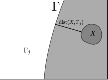
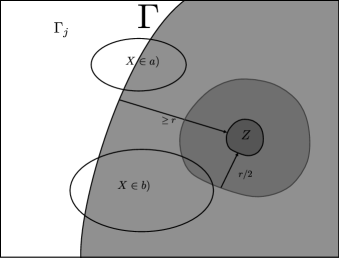
The result is that local restrictions of any ground state of approach the local restriction of fast, as a function of the distance to the impurity or boundary region , see also Figure 1.
Informal claim on local stability: There is a stretching exponent and finite constant such that, for any ground state of , and for any local observable supported in with ,
As far as we can see, there is no natural sense in which resembles , other than what is expressed in this claim. In particular, is not necessarily the unique ground state, it has in general no gap111Actually, our assumptions do not explicitly require a global gap for either, but such a gap is there in spirit because of the invertibility assumption, and we have left it in the abstract to fix thoughts., no short range entanglement properties and it is not frustration-free. To illustrate this, in particular the possibility of long-range entanglement, we consider and we imagine that at each site there is a qubit, i.e. a two-dimensional Hilbert space, with base states . The Hamiltonian is where acts at site , as and . This Hamiltonian has a unique ground state that is a product, namely . The perturbation is chosen as with some and a two-qubit operator acting on sites and . Because of the very small prefactor , this perturbation satisfies any reasonable locality requirement. By taking , the perturbed system has 4-fold ground state degenerary. By taking to be minus the rank-1 projector on the entangled Bell state , the perturbed system has a unique ground state that has maximal entanglement between qubits and .
1.1 Discussion
1.1.1 Spectral stability of the ground state sector
The above result should be contrasted with recent work on the stability of the spectral gap against locally small perturbations. That recent work can be split in two classes. The first class concerns systems where the unperturbed ground state is a product, see [1, 2, 3, 4, 5, 6, 7]. The second class is based on the so-called Bravyi-Hastings-Michalakis (BHM) argument which applies to frustration-free ground states, see [8, 9, 10, 11]. Both classes are eventually based on some form of spectral perturbation theory applied to the ground state sector. In all of the above cases, one also obtains some form of locality for the action of small perturbations, captured by the slogan ‘local perturbations perturb locally’, see also [12, 13].
Our result is different in spirit, as our perturbations are not assumed to be small, but we obtain only information about the perturbed ground states in regions far away from the region where the perturbation acts. On the other hand, and in contrast to the quoted works, our result relies crucially on the variational principle and so it holds only for ground states (or ceiling states). One should realize that it is not only the proof of the results in [8, 9, 10] that does not apply in our case, but also the results should not be expected, as already stressed above through an example.
1.1.2 Role of the invertibility assumption
If one drops the invertibility assumption, then the claim on local stability in Section 1 can no longer hold. To see this, one can consider the two-dimensional toric code model [14, 15] on a large square . This model is frustration-free and with appropriate boundary conditions, there is a unique groundstate . The OBC restrictions always have a spectral gap that is bounded below by a positive constant, and the topological order condition holds. However, the state is not invertible, regardless of boundary conditions. The lack of invertibility is associated with anyonic excitations that are created in pairs. By choosing a boundary condition that fixes a single anyon excitation at the boundary of a region , one forces a partner anyon to be present somewhere in the interior of , see Figure 2. In this case, there will be multiple ground states, labelled by the position of the partner anyon. Since can be arbitrarily far from the boundary, the claim on local stability does not hold.
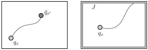
Of course, the large degeneracy of ground states is not a robust feature of the model. Indeed, if one adds a small global perturbation to the model, which will in general give the hitherto static anyons some mobility (see e.g. [16]), then the degeneracy will be lifted and the unique ground state will correspond to a delocalized anyon. In this case, the claim on local stability is still violated because the ground state now differs locally from by an amount that is an inverse polynomial in the volume .
1.1.3 Remaining assumptions, extensions, and related results
As argued above, the invertibility assumption can not be dropped. We can also not drop the LTQO condition. Consider for example acting on the chain of qubits (as the example immediately below the informal claim). We take the classical Ising Hamiltonian such that its ground states exhibits spontaneous symmetry breaking, with ground states and . The term breaks the symmetry at the boundary, so that has a unique ground state . In that case our result does not hold, as we see by taking . The LTQO assumption fails to hold since in the interior of , the symmetry remains unbroken and the OBC restrictions in the interior also have as ground states. Of course, one could imagine replacing the LTQO condition by some form of translation invariance of the Hamiltonian , ruling out the above example.
Apart from this, we do not see that the other assumptions are fundamentally necessary, though they are necessary for our proof. However, a mild extension of our result seems within reach: we hope that techniques introduced within the BHM argument, see Section 1.1.1, could allow to generalize our result in the following way: If we were to tighten our assumptions so that the local gap , i.e. the local gap is uniformly bounded from below, then the result should also hold for Hamiltonians of the type where and its ground state satisfy the tightened assumptions, is a Hamiltonian with the same locality restrictions as and , and is a small parameter.
Results similar to ours have recently been obtained independently in [17], as a corollary to [4]. The result of [17, 4] yields full exponential decay and requires no explicit frustration freeness, but it is restricted to weakly interacting spins, i.e. perturbations of products. Instead, our result relies on the automorphic equivalence of the unperturbed ground state to a product state, possibly upon adjoining an auxiliary state. Both results need hence an underlying product structure. Another line of research that is loosely connected to ours, concerns stability at nonzero temperature in spatial dimension 1, see [18, 19].
Acknowledgements
W.D.R thanks Marius Schütz and Simone Warzel for collaboration and discussions of many years ago that proved crucial for the present paper. We thank two anonymous referees for very constructive remarks that allowed us to substantially improve the paper, in particular concerning the necessity of the assumptions. M.F. was supported in part by the NSF under grant DMS-1907435. W.D.R. was supported in part by the FWO under grant G098919N. S.B. was upported by NSERC of Canada.
2 Setup
2.1 Preliminaries
2.1.1 Spatial structure
We consider a finite graph , equipped with the graph distance . Let be the ball of radius centered at . The graph is assumed to have a finite dimension , i.e. there is a such that
For reasons of recognizability, we refer to vertices as ‘sites’. To every site is associated a finite-dimensional Hilbert space and we define the total Hilbert space and the algebra of bounded operators on . For any , we have the Hilbert space and the algebra . We use the usual embedding given by . As is customary, we will identify with and say that is supported in .
2.1.2 Locality
We write for the strictly positive naturals and we let be a class of functions of quasi-exponential decay. The class is defined by the following two conditions.
-
1.
is non-increasing.
-
2.
For every , there exists such that .
Note that the same class of functions is obtained by setting , which is used often in the proofs. To express the locality properties of Hamiltonians, we consider collections of local terms , sometimes called ’interactions’, and we endow them with a family of norms, parametrized by :
The locality property is then expressed by the finiteness of for some .
2.1.3 Trace norms
We denote by the trace on the Hilbert space , and we abbreviate , i.e. the trace on the global Hilbert space . We recall the trace norm on , defined by
We then denote by the partial trace , satisfying for any . Since we will often use trace norms of operators resulting from the partial trace we introduce a short-hand notation:
Nonnegative operators on that have unit trace , are called density matrices and we write for . For , we write for the pure density matrix equal to the orthogonal projector on .
2.2 Spaces and Hamiltonian
The Hamiltonian and the perturbation are written as
| (1) |
The perturbation is spatially restricted to a region in a mild sense
Then, we assume, for the collections ,
for some .
2.3 Assumptions
Our first assumption states that the Hamiltonian has a frustration free ground state , i.e. is an eigenvector of with eigenvalue equal to ( is the spectrum). Our conventions are such that this eigenvalue is .
Assumption 1 (Frustration-free ground state).
All the terms are nonnegative: . There is a such that for any . We denote by the corresponding density matrix.
We note that the frustration free property depends on the way the Hamiltonian is written as a sum of local terms, i.e. on the interaction. Next, we introduce ‘open boundary condition’ (OBC) restrictions of ,
Just as the frustration free property, the notion of OBC restriction depends on the interaction. We let be the orthogonal projector on . Since , it holds that
and hence also
The following assumption has come to be known as ‘Local Topological Quantum Order’ (LTQO) but, in our case, it is better described as the property that the density matrix of any ground state of the OBC Hamiltonian looks similar to the global ground state in the deep interior of . Recall that is the ball or radius centered at .
Assumption 2 (OBC-regularity).
There is and such that, for any and ,
Let us briefly comment on the precise form of the above bound. We have in mind, roughly, that any differs from only through the presence of boundary modes. One realization of this would be that any such is of the form with a sum of terms supported near the boundary of . This would indeed lead to the bound above with chosen such that .
The next assumption concerns the local gap of OBC Hamiltonians. Let
be the spectral gap of .
Assumption 3 (Local Gap).
There are such that, for any
This assumption 3 might be misleading. In most examples of models with gapped frustration-free ground states, that we are aware of, OBC restrictions have a gap that is actually bounded below in , and the physical edge modes are found as ground states of , i.e. the eigenvalue at will typically be degenerate. In that case, the genuine restriction is not so much assumption 3 but rather assumption 2 which describes the kernel .
2.3.1 Invertibility
Let be with finite-dimensional Hilbert spaces. We will now consider the tensor product which we denote by
The superscript reminds us of the fact that this is not a tensor product between disjoint spatial regions, but between the ‘original’ Hilbert space and an ‘auxiliary’ Hilbert space. This is helpful because we also view again as a tensor product over sites
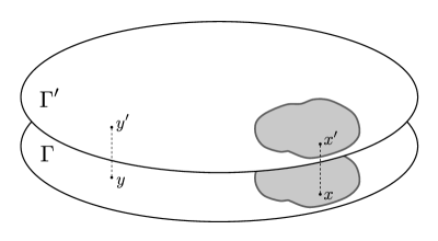
The local structure of the space is analogous to the one of , except that now the dimension of the on-site spaces is larger, see Figure 3. We consistently put a prime on algebras derived from , and we put a tilde on algebras derived from , i.e. and are subalgebras of operators supported in . We also copy the definition of collections of local operators and their norms , simply replacing by . The next assumption expresses that the state has no long-range entanglement. Loosely speaking, one could describe this assumption as ‘upon adjoining an auxiliary state , is automorphically equivalent to a product state’ [12, 20].
Assumption 4 (Invertibility).
There are collections of local operators , indexed by , such that
-
1.
and is measurable, for any .
-
2.
for some .
-
3.
There is a product state and a state such that
where .
We say that is an ‘inverse’ to .
The ‘invertibility’ assumption roughly corresponds to states that do not have anyonic excitations. Examples of invertible states are: symmetry protected topological states (SPT’s) [21, 22, 23], states characterized by an integer quantum Hall effect [24], etc.. We refer to the extensive literature for a more thorough discussion. The motivation for considering the type of spatial decay expressed by the class is because this corresponds to the decay one can prove for the spectral flow connecting ground states of a uniformly gapped Hamiltonian, by the technique of (quasi-)adiabatic continuation, see [20, 12].
2.4 Result
We say that a unit vector is a ground state of the perturbed Hamiltonian if is an eigenvector of with eigenvalue equal to . Recall that is the density matrix associated to , the distinghuished ground state of the unperturbed Hamiltonian , and is the density matrix associated to . By a ‘constant’, we mean a quantity that can depend only on , the numbers and . In particular, constants can not depend on the sizes and .
Theorem 1.
For any , there is a constant such that, for any ground state of , and any , with ,
To connect this theorem to the informal claim on stability in Section 1, note that the left hand side is equal to with .
3 Proof of Theorem 1
We define some additional notation to be used in this section. For regions , we define the fattening
(we will simply write when no confusion is possible) and the boundary
We use constants as introduced just before Theorem 1, i.e. depending on a number of fixed parameters. Sometimes we write to indicate that can additionally depend on a parameter . We also use the generic notation for a function in that depends possibly on those same fixed parameters. Just as the constants , the precise function can change from line to line. In the same vein, we also use to denote a polynomial that depends only on the fixed parameters.
3.1 Stitching maps
Recall that is the global ground state density matrix of the unperturbed Hamiltonian . We say that a family of maps , indexed by , are stitching maps if the they satisfy the following properties.
Definition 1.
Stitching maps with are trace-preserving completely positive maps iff. there is an such that, for any and any density matrices on ,
-
1.
-
2.
-
3.
To state this in a rough way, stitching maps are such that and further
The stitching maps will be used for regions that are far away from the perturbation region .
The purpose of the invertibility assumption 4 is precisely to ensure the existence of stitching maps, as we show now. Recall that is the enlarged Hilbert space.
Proposition 1.
We first construct the appropriate unitaries featuring in Proposition 1. To that end, we introduce the truncated interactions by
with as given in assumption 4. We let be the unitary defined analogously to in the invertibility assumption 4, but with replaced by . We then set
and we observe that
| (3) |
for some . This shows that satisfies property 3) of definition 1. The full proof of Proposition 1, i.e. the verifications of properties 1) and 2) of definition 1, uses some standard terminology and locality estimates that are not needed in the rest of our proof, hence we postpone them to the appendices, but we do state the relevant locality property of the unitary operators . To that end, let us introduce the conditional expectation, for any ,
Lemma 1.
For any regions and , with as defined above,
| (4) |
and
| (5) |
The same estimates hold• as well if we exchange and .
The proof of Lemma 1 follows from well-known considerations based on Lieb-Robinson bounds, and it is sketched in Appendix B. Finally, the proof of properties 1) and 2) of definition 1 is an intuitive consequence of Lemma 1. This proof is given in Appendix A.
3.1.1 Action of a stitching map at the stitch
We will now establish a property of stitching maps, which we will henceforth denote by , that relies crucially on the OBC-regularity assumption 2. It makes explicit that stitching maps are ‘seamless’, i.e. they do not introduce errors at the cut . Recall that is the ground state projector corresponding to the OBC restriction and let .
Proposition 2.
Let be the pure density matrix associated to some . Consider a set and balls for some site . Then (recall that is a polynomial),
Proof.
Since will be fixed, we drop it and write . Let us denote and remark that . If , then the required bound is trivial, hence we assume . We split
We will treat these terms separately, i,e. find bounds on
The term
Since ,
and we can define
the pure density matrix , satisfying .
By the properties of definition 1, we get the equality and first inequality in
whereas the last inequality follows from the OBC regularity assumption 2. By the frustration-free property, , and thus the above inequality yields . Since , this implies
The term
Here we have
and since is trace-preserving,
The term
Since is pure, we can write
and we note that . To estimate , we use Lemma 2 below to get
The second inequality follows from the bound for the term above.
Lemma 2.
For an orthogonal projector , a trace-conserving CP map and , we have
Proof.
Introducing the adjoint map , the first inequality reads
It follows from positivity of and the Cauchy-Schwarz inequality. ∎
The term
The bound and its proof are analogous to the case of .
The claim of the lemma follows by adding the bounds on for .
∎
3.2 A bound on the energy increase due to stitching
If we apply the stitching map to a pure density matrix , we expect its energy (associated to ) to decrease in the far interior of and to remain unchanged far outside . Around the stitch , the energy can of course increase. In the present section we prove that this energy increase is upper bounded by the energy of around the stitch. We make this precise in Lemma 3. The proof is based largely on Proposition 2 that allows us to convert a bound on the energy to a bound on the local deviation from .
Lemma 3.
Let be a pure density matrix, i.e. for some , and let for some region . Then
Proof.
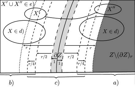
We split the class of contributing the left hand side222The condition appearing in the statement of the lemma, is actually irrelevant for its validity. in disjoint classes :
-
-
-
and .
-
and .
-
and and .
We will now estimate, with ,
| (6) |
-
class
The first inequality follows from non-negativity of . The second from property 1) of definition 1 and the third from . Then we use and the rapid decay of to absorb a polynomial factor in .
-
class
The first inequality is property 1) of definition 1, the rest is analogous to case above.
-
class
The first and second inequality is by nonnegativity of . The third inequality uses for , i.e. the frustration freeness of assumption 1, and . The fourth inequality uses Proposition 2. The fifth inequality is by the local gap assumption 3. The sixth inequality follows because any is included in at most a number of balls with radius . For the last inequality, we use and we absorbed the polynomial in .
-
class
The first inequality follows from . Then we use analogous reasoning as for class .
-
class
The reasoning is analogous to that for class and class .
∎
The previous Lemma 3 was only concerned with the unperturbed Hamiltonian . We now state an analogous estimate for the Hamiltonian .
Lemma 4.
Let be a density matrix and let be a set such that . Then
| (7) |
Proof.
We estimate
. We split the sets into two disjoint classes:
We estimate the contribution of each class and we get in each case the desired bound.
-
class
We use property 1 of definition 1 to get the first inequality. The last inequality follows by the rapid decay of and the fact that has finite dimension .
-
class
The first inequality follows because unless . In the last inequality, we again absorbed a polynomial factor in .
∎
3.3 Isoperimetry
From now on, we assume that with a ground state of . In particular, this means that the following inequality holds:
| (8) |
We will use Lemma’s 3 and 4 to relate the energy in a region to the energy around , which explains the title of this subsection. We again choose the region to be far away from : with . By Lemma 4, we can discard in the above inequality at small cost, and we obtain
| (9) |
We split this inequality as
| (10) |
from which we get
Lemma 5.
Proof.
Let us now put Lemma 5 to use. We will consider a sequence of regions chosen as concentric balls , with fixed and to be specified. We note that
and we abbreviate
Then, the inequality in Lemma 5 reads
| (11) |
Note also that provided that . Our strategy will be to establish a lower bound on , depending on , and then eventually use the a priori upper bound
to get an upper bound on . Proceeding in this way, we obtain
Lemma 6.
Let with the center of the balls above. Then, for any
Proof.
We choose for with the largest integer that is smaller than . Using inequality (11) and we obtain
| (12) |
where we also updated the function compared to (11). We will now use a Grönwall-type inequality. Multiplying the inequality (12) by and summing over yields
which implies
and hence, choosing ,
To estimate the sum on the right hand side, we bound and estimate
Using in addition the a priori bound , we get
To optimize the inequality we let grow with , namely . For and , we can find such that and we get hence
which is the claim of the lemma, since .
∎
Proof of Theorem 1.
We recall that with a ground state of . By the local gap assumption 3, we have
and by Lemma 6, we then get, for any ,
| (13) |
From (13) we get, with and for large enough, , and setting , we get . From this one bounds ( is the global trace norm)
Since , the OBC regularity assumption 2 allows us to bound
with a polynomial. We choose . Then we get, for any
This yields the statement of Theorem 1. ∎
Appendix A Appendix: Locality properties of CP maps
We establish some vocabulary that is helpful for the proof of Proposition 1.
A.1 Completely positive maps
We consider completely positive (CP) maps acting from to , with finite-dimensional Hilbert spaces. We need identity-preserving CP maps and trace-preserving CP maps, which are dual to each other. Let be an identity preserving CP map, then the adjoint trace-preserving CP map is defined by
From the Russo–Dye theorem, it follows that identity preserving CP maps are contracting w.r.t. operator norm: and trace-preserving CP maps are contracting w.r.t trace norm with , cf. the notation in Section 2.1.3.
A.2 Conditional expectations
Let us consider a bipartite finite-dimensional Hilbert space . For any density matrix on , we can define the conditional expectation
Note that is an identity-preserving CP map and that its range is which is naturally identified with . Its adjoint is
| (14) |
Let be the density matrix on , i.e. corresponds to the tracial state on . The case where is or for some , and is of special signficance to us and we denote the corresponding conditional expectation simply by . This is consistent with the usage of the symbol in Lemma 1.
A.3 Almost locality preserving CP maps
We consider identity-preserving CP maps , acting between (subalgebras of) , i.e. there is a spatial structure. We say that preserves almost locality if there exists such that,
| (15) |
where is the conditional expectation using the tracial state on , as discussed above. A useful property is that, if preserve almost locality (say, with functions ) then so does . Indeed, for ,
| (16) | ||||
| (17) | ||||
| (18) |
Using that are norm-contracting and almost locality preserving, and that the image of is in , the error terms are bounded as
Since and also is norm-contracting, we verify that the overall error term is of the form , and hence indeed preserves almost locality.
A.4 Verification of properties 1) and 2) of definition 1
We study the the trace-preserving map , defined in Proposition 1, via its adjoint , an identity-preserving CP map. We decompose with the identity-preserving CP maps given below.
-
:
-
:
-
:
with the density matrix on .
-
:
-
:
-
:
with the density matrix on .
Each of the maps preserves almost locality, i.e. satisfies (15). This is immediate for with , whereas for it is a consequence of the bound (4) in Lemma 1. Hence, by duality, we obtain that the locality property (19) is satisfied for , the map from Proposition 1. We then write, for any density matrices ,
| (20) |
The first two terms on the right-hand side are bounded in -norm by (19) with . The last term is bounded as
where we used in particular contractivity of . This yields property 2) of definition 1. To check property 1) of definition 1, we compare the action of on with far from with the action of the identity map. By the bound (5) in Lemma 1, we have,
The verification of property 1) now follows by similar reasoning as for property 2).
Appendix B Appendix: Locality estimates
We review the standard propagation bounds that are necessary for the proof of Lemma 1. These bounds go back to [25] but we use the recent formulation in [26]. There are a few differences in our treatment compared to [26]. Most importantly, we have an underlying finite graph equipped with the graph distance, and we always assume that this graph has a finite spatial dimension as defined in Section 2.1.1.
B.1 Norms on interactions
In the main text, we defined a family of norms with . In [26], as in many preceding works, another family of norms is used, which we introduce now. Namely, one defines so-called -functions as functions satisfying
-
1.
is non-increasing.
-
2.
There is such that, for all ,
-
3.
There is such that, for each , .
Strictly speaking, the latter two properties are of course empty for a finite graph , but we have in mind that these properties holds for constants that can be chosen uniform in . This is consistent with the conventions used in the main text, as explained in Section 2.4.
Then we can define a family of corresponding norms on interactions.
(Note that we use the symbol to distinghuish these norms from the norms in the main text). If we work with functions decaying faster than polynomials, one can switch back and forth between the norms and , as we state in the next lemma. In stating the comparison, we write meaning that (The functions in the main text are defined on whereas the functions are defined on .)
Lemma 7.
For any , there is an -function in such that
For any -function , there is a such that
To prove this, we need the following observation
Lemma 8.
Let be a function such that for any , then there is an -function such that for any .
Proof.
We say a function is logarithmically superadditive if
| (21) |
Following [27], we define the following transformation of functions :
This transformation has the following properties
-
1.
is logarithmically superadditive.
-
2.
If , then . In particular, .
-
3.
If is logarithmically superadditive, then .
Let now satisfy the assumption of the lemma and put with such that . Then, we put
and . Then is an -function (such properties are extensively discussed in [26]) and, by property 2) above, . It remains to show that has sufficiently rapid decay. Since and , we can find such that . Since , is logarithmically superadditive, we have
Therefore, and hence have indeed sufficiently rapid decay and we conclude that . ∎
Proof of Lemma 7.
To get the first claim we observe
| (22) | ||||
| (23) | ||||
| (24) |
In order to have the last expression dominated by , we need to choose the -function such that . The possibility of doing this was argued in Lemma 8. For the second claim, we write
In order to have the last expression dominated by , we need to choose such that, for all , , and hence,
The function is not necessarily non-increasing, which is remedied by setting
We can now check that as it inherits the rapid decay from . ∎
We call the set of interactions with finite -norm and , with a (possibly infinite) interval, the set of time-dependent interactions , with finite norm
and such that is measurable for all . Pointwise addition of interactions makes and into Banach spaces w.r.t. the norm .
B.2 Locally generated automorphisms
Let and let with . We let be the dynamics (a family of automorphisms or ) generated by the family acting from time to time , in the sense that
Since is finite, the existence and uniqueness of this dynamics follows from elementary facts on matrix-valued ODE’s. For , one often abbreviates
as we did in the main text. We first state a version of the Lieb-Robinson bound, using the language introduced in Section 2.1.
Theorem 2 (Lieb-Robinson bound).
Let , and let with . Let with . Then
This is a slightly weakened form of Theorem 3.1 in [26], except for two details. Our graph is finite and we allow our time-dependent interaction to be composed of measurable functions for any . Inspection of the proof in [26] confirms that this is all what is needed.
The Lieb-Robinson bound does not directly address the question how to write the evolved observable as a sum of local terms. A natural way to do this is to use the conditional expectation as defined in Section 3.1. If , then we can write
| (25) |
where the maps are defined as
and we recall that . We see that the terms corresponding to in the sum in (25) are supported on the fattened sets . The Lieb-Robinson bound can then be used to provide bounds on the right-hand side of (25) via the following standard lemma, whose proof we omit.
Lemma 9.
For any ,
B.2.1 Evolution of interactions
Let be an interaction and recall that we associate to it a Hamiltonian
Let now be as above, i.e. a time-dependent interaction, determining a family of autormorphisms . We can use these autormorphisms to obtain a new Hamiltonian by transforming into . It is very intuitive that this Hamiltonian can again be expressed as a sum of local terms with good decay properties in the size of the support, i.e. we can express the Hamiltonian as the Hamiltonian corresponding to an new interaction that we then view as a time-evolved interaction . A priori, there are multiple ways to define since there are multiple ways to represent an operator as a sum of local terms. For convenience, we follow [26] and set
using the operators introduced above. This definition has the following convenient properties
-
1.
.
-
2.
If is anchored in a set , then is also anchored in .
-
3.
If the -functions are in , then there is an -function depending only on , such that
(26)
The first two properties follow immediately from the definitions. The third property is derived starting from the Lieb-Robinsin bound. For details we refer to [26], where one can find explicit choices for .
This enables us to define many new time-dependent interactions in Lemma 10. To set the stage, we first define the ”commutator” of two interactions as
We note that if either one of is anchored in a set , then the commutator is also anchored in . Then we can establish
Lemma 10.
Let be time-dependent interactions in , respectively, with . Then the following interactions are in , with and depending only on (for item 1)) and on (for items 2,3),
-
1.
-
2.
-
3.
The time-dependent interaction in item 1) satisfies
| (27) |
The time-dependent interaction in item 3) satisfies
| (28) |
Sketch of proof.
First, one verifies that the newly defined time-dependent interactions satisfy the measurability condition, using that do so. Then, the bound on follows directly from (26). The identities (27) and (28) follow by direct computation. The bound on follows by combining all the previous items, i.e. the fact that commutators, time-evolution and inverse time-evolution map into for certain . ∎
On our way to prove Lemma 1, we first state the following observation concerning the unitary family introduced in the proof of Proposition 1 in the main text.
Lemma 11.
There is an -function and a time-dependent interaction such that
| (29) |
Moreover, is anchored in .
Proof.
We recall the time-dependent interactions . These were defined as having a finite norm, with . By Lemma 7, we find an -function such that have a finite -norm. From the definition of , we deduce that
We set
and we note that is anchored in , for any . Now we invoke item 3) of Lemma 10, with , to conclude that there is , given by
such that . Since commutators and time-evolution preserve the property of being anchored in a set, we conclude that , just as , is anchored in . ∎
B.3 Proof of Lemma 1
For convenience we restate Lemma 1:
Lemma 12 (repetition of Lemma 1).
For any regions and , with as in Lemma 11 above,
| (30) |
and
| (31) |
The same estimates hold as well if we exchange and .
To get the bound (30), we invoke Lemma 11 and Lemma 9 to relate conditional expectations to commutators. Then, we use the Lieb-Robinson bound (Theorem 2) for the dynamics :
The last expression between brackets is estimated as , since and the spatial dimension is finite.
Let us now turn to (31). By the Heisenberg equation,
Therefore, we can bound
The third line follows because is supported in and is anchored in . The expression in the last line is dominated by upon using that , that the spatial dimension is finite, and bounding by a constant.
References
- [1] Wojciech De Roeck and Marius Schütz. “An exponentially local spectral flow for possibly non-self-adjoint perturbations of non-interacting quantum spins, inspired by kam theory”. \hrefhttps://dx.doi.org/10.1007/s11005-016-0913-zLetters in Mathematical Physics 107, 505–532 (2017).
- [2] Simone Del Vecchio, Jürg Fröhlich, Alessandro Pizzo, and Stefano Rossi. “Lie-schwinger block-diagonalization and gapped quantum chains: analyticity of the ground-state energy”. \hrefhttps://dx.doi.org/10.1016/j.jfa.2020.108703Journal of Functional Analysis 279, 108703 (2020).
- [3] Juerg Froehlich and Alessandro Pizzo. “Lie–schwinger block-diagonalization and gapped quantum chains”. \hrefhttps://dx.doi.org/10.1007/s00220-019-03613-2Communications in Mathematical Physics 375, 2039–2069 (2020).
- [4] DA Yarotsky. “Ground states in relatively bounded quantum perturbations of classical lattice systems”. \hrefhttps://dx.doi.org/10.1007/s00220-005-1456-9Communications in mathematical physics 261, 799–819 (2006).
- [5] Nilanjana Datta, Roberto Fernández, and Jürg Fröhlich. “Low-temperature phase diagrams of quantum lattice systems. i. stability for quantum perturbations of classical systems with finitely-many ground states”. \hrefhttps://dx.doi.org/10.1007/BF02179651Journal of statistical physics 84, 455–534 (1996).
- [6] Christian Borgs, R Koteckỳ, and D Ueltschi. “Low temperature phase diagrams for quantum perturbations of classical spin systems”. \hrefhttps://dx.doi.org/10.1007/BF02101010Communications in mathematical physics 181, 409–446 (1996).
- [7] Matthew F Lapa and Michael Levin. “Stability of ground state degeneracy to long-range interactions” (2021). \hrefhttp://arxiv.org/abs/2107.1139arXiv:2107.11396.
- [8] Sergey Bravyi, Matthew B Hastings, and Spyridon Michalakis. “Topological quantum order: stability under local perturbations”. \hrefhttps://dx.doi.org/10.1063/1.3490195Journal of mathematical physics 51, 093512 (2010).
- [9] Spyridon Michalakis and Justyna P Zwolak. “Stability of frustration-free hamiltonians”. \hrefhttps://dx.doi.org/10.1007/s00220-013-1762-6Communications in Mathematical Physics 322, 277–302 (2013).
- [10] Bruno Nachtergaele, Robert Sims, and Amanda Young. “Quasi-locality bounds for quantum lattice systems. part ii. perturbations of frustration-free spin models with gapped ground states”. In Annales Henri Poincaré. \hrefhttps://dx.doi.org/10.1007/s00023-021-01086-5Volume 23, pages 393–511. Springer (2022).
- [11] Bruno Nachtergaele, Robert Sims, and Amanda Young. “Stability of the bulk gap for frustration-free topologically ordered quantum lattice systems” (2021). \hrefhttp://arxiv.org/abs/2102.0720arXiv:2102.07209.
- [12] Sven Bachmann, Spyridon Michalakis, Bruno Nachtergaele, and Robert Sims. “Automorphic equivalence within gapped phases of quantum lattice systems”. \hrefhttps://dx.doi.org/10.1007/s00220-011-1380-0Communications in Mathematical Physics 309, 835–871 (2012).
- [13] Wojciech De Roeck and Marius Schütz. “Local perturbations perturb—exponentially–locally”. \hrefhttps://dx.doi.org/10.1063/1.4922507Journal of Mathematical Physics 56, 061901 (2015).
- [14] Alexei Kitaev. “Anyons in an exactly solved model and beyond”. \hrefhttps://dx.doi.org/10.1016/j.aop.2005.10.005Annals of Physics 321, 2–111 (2006).
- [15] Alexei Kitaev and Chris Laumann. “Topological phases and quantum computation”. Exact methods in low-dimensional statistical physics and quantum computing, Lecture Notes of the Les Houches Summer SchoolPages 101–125 (2009). url: \hrefhttps://arxiv.org/pdf/0904.2771.pdfarxiv.org/pdf/0904.2771.pdf.
- [16] Bruno Nachtergaele and Nicholas E Sherman. “Dispersive toric code model with fusion and defusion”. \hrefhttps://dx.doi.org/10.1103/PhysRevB.101.115105Physical Review B 101, 115105 (2020).
- [17] Joscha Henheik, Stefan Teufel, and Tom Wessel. “Local stability of ground states in locally gapped and weakly interacting quantum spin systems”. \hrefhttps://dx.doi.org/10.1007/s11005-021-01494-yLetters in Mathematical Physics 112, 1–12 (2022).
- [18] Matthew B Hastings. “Quantum belief propagation: An algorithm for thermal quantum systems”. \hrefhttps://dx.doi.org/10.1103/PhysRevB.76.201102Physical Review B 76, 201102 (2007).
- [19] Kohtaro Kato and Fernando GSL Brandao. “Quantum approximate markov chains are thermal”. \hrefhttps://dx.doi.org/10.1007/s00220-019-03485-6Communications in Mathematical Physics 370, 117–149 (2019).
- [20] Matthew B Hastings and Xiao-Gang Wen. “Quasiadiabatic continuation of quantum states: The stability of topological ground-state degeneracy and emergent gauge invariance”. \hrefhttps://dx.doi.org/10.1103/PhysRevB.72.045141Physical review b 72, 045141 (2005).
- [21] Daniel S Freed. “Anomalies and invertible field theories”. In Proc. Symp. Pure Math. Volume 88, pages 25–46. (2014). url: \hrefhttps://arxiv.org/pdf/1404.7224.pdfarxiv.org/pdf/1404.7224.pdf.
- [22] A. Kitaev. “On the classification of short-range entangled states”. http://scgp.stonybrook.edu/video_portal/video.php?id=2010.
- [23] Zheng-Cheng Gu and Xiao-Gang Wen. “Tensor-entanglement-filtering renormalization approach and symmetry-protected topological order”. \hrefhttps://dx.doi.org/10.1103/PhysRevB.80.155131Physical Review B 80, 155131 (2009).
- [24] Anton Kapustin and Nikita Sopenko. “Hall conductance and the statistics of flux insertions in gapped interacting lattice systems”. \hrefhttps://dx.doi.org/10.1063/5.0022944Journal of Mathematical Physics 61, 101901 (2020).
- [25] E.H. Lieb and D.W. Robinson. “The finite group velocity of quantum spin systems”. \hrefhttps://dx.doi.org/10.1007/978-3-662-10018-9_25Commun. Math. Phys. 28, 251–257 (1972).
- [26] Bruno Nachtergaele, Robert Sims, and Amanda Young. “Quasi-locality bounds for quantum lattice systems. i. lieb-robinson bounds, quasi-local maps, and spectral flow automorphisms”. \hrefhttps://dx.doi.org/10.1063/1.5095769Journal of Mathematical Physics 60, 061101 (2019).
- [27] A. Bruckner. “Minimal superadditive extensions of superadditive functions”. Pacific J. Math. 10, 1155–1162 (1960). url: \hrefhttps://msp.org/pjm/1960/10-4/pjm-v10-n4-s.pdf#page=51msp.org/pjm/1960/10-4/pjm-v10-n4-s.pdf#page=51.
