Asymptotics of cut distributions and robust modular inference using Posterior Bootstrap

Abstract

Bayesian inference provides a framework to combine an arbitrary number of model components with shared parameters, allowing joint uncertainty estimation and the use of all available data sources. However, misspecification of any part of the model might propagate to all other parts and lead to unsatisfactory results. Cut distributions have been proposed as a remedy, where the information is prevented from flowing along certain directions. We consider cut distributions from an asymptotic perspective, find the equivalent of the Laplace approximation, and notice a lack of frequentist coverage for the associate credible regions. We propose algorithms based on the Posterior Bootstrap that deliver credible regions with the nominal frequentist asymptotic coverage. The algorithms involve numerical optimization programs that can be performed fully in parallel. The results and methods are illustrated in various settings, such as causal inference with propensity scores and epidemiological studies.

1 Introduction

1.1 Cutting feedback in Bayesian models

Bayesian models are often built of different components or “modules”, which can represent different sources of information about the studied phenomenon. Standard Bayesian inference relies on samples from the posterior distribution over the joint model combining all modules, and this approach is optimal when the model is well-specified [Zellner, 1988, Bissiri et al., 2016]. In many applications, however, the analyst suspects that some or all modules may be misspecified. Such cases motivate departures from the joint model. In particular, it may be beneficial to cut the flow of information from the module that we put less trust in, to the ones that we trust more.

The issue described above often arises in pharmacology. Pharmacokinetics-pharmacodynamics (PK/PD) models combine data from two sources. They have a PK component, considering the body’s effect on a drug, and a PD module, focusing on the effect the drug has on the body. Pharmacokinetics is believed to be better understood scientifically, which gives researchers more trust in the PK part of the model, while PD components are often suspected to be misspecified. Therefore, instead of relying on the full model, researchers doing PK/PD analysis often first fit the PK model, and then use the estimated parameters as input for the PD module, thus cutting the feedback from the PD component to the PK one [Zhang et al., 2003a, b, Lunn et al., 2009]. We will refer to this approach as modular Bayesian inference, but it is also known in the literature as “modularized” approach [Liu et al., 2009] or “cutting feedback” [Plummer, 2015]. In econometrics similar situations are commonly tackled with “two-stage” procedures [Murphy and Topel, 2002].

Apart from the PK/PD models, the modular approach is commonly used in econometrics, for example, when errors from one regression model are used as a covariate in another model. It has also been useful for epidemiological models [Maucort-Boulch et al., 2008], studies on health effects of air pollution [Blangiardo et al., 2011], analysis of computer models and meta-analysis [Liu et al., 2009]. Another situation where two-stage estimation is routinely used is Bayesian inference based on a dataset where missing data were first imputed, e.g. with “multiple imputation” [Little, 1992, Rubin, 2004, Zhou and Reiter, 2010].

Furthermore, cutting feedback is an established practice in causal inference. To estimate the average treatment effect from observational data, the user needs to account for confounding variables in the dataset, which can be done using propensity scores. Recall that in randomized trials the treatment assignment happens before the outcome is known, whereas in observational studies propensity scores are used to compensate for the lack of randomized treatment assignment. This, apart from potential misspecification, is another reason for choosing the two-step approach. The first stage of the analysis aims to estimate propensity scores, given a set of covariates but not using the outcome, whereas the second stage focuses on estimating the treatment effect on the outcome, given the covariates and stratified by propensity scores. As shown by Zigler et al. [2013], performing the full Bayesian inference is possible, but leads to bias in the estimation of causal effects; see also Zigler [2016]. A review of various applications of modular inference is presented in Jacob et al. [2017].

Throughout the paper we will write $y_{1},\ldots,y_{n}\sim f(y|\theta)$ to denote that observations $y_{1},\ldots,y_{n}$ are independent and identically distributed according to a distribution with density $f(y|\theta)$. Formally, we will study the following model:

$$x_{1,1},\ldots,x_{1,n_{1}} \sim f_{1}(x_{1}|\theta_{1}), \theta_{1} \sim\pi_{1}(\theta_{1}),\quad\theta_{1}\in\Theta_{1}\subseteq\mathbb{R}^{d_{1}},$$ (1)

$$x_{2,1},\ldots,x_{2,n_{2}} \sim f_{2}(x_{2}|\theta_{1},\theta_{2}), \theta_{2} \sim\pi_{2}(\theta_{2}),\quad\theta_{2}\in\Theta_{2}\subseteq\mathbb{R}^{d_{2}}.$$

In the first module the likelihood $f_{1}$ depends only on $\theta_{1}$, whereas the second likelihood $f_{2}$ depends both on $\theta_{1}$ and $\theta_{2}$. Distributions $\pi_{i}$ denote the priors on $\theta_{i}$, for $i=1,2$. The analyst may alternatively consider the prior distribution in the second module as dependent on $\theta_{1}$, that is, to define it as $\pi_{2}(\theta_{2}|\theta_{1})$; the findings of the present article are easily adapted to that more general setup. By $x_{i,1:n_{i}}$, $i=1,2$, we denote the vector of observations $x_{i,1},\ldots,x_{i,n_{i}}$.

The full posterior distribution associated with model (1) is given by

$$\begin{split}\pi(\theta_{1},\theta_{2}&|x_{1,1:n_{1}},x_{2,1:n_{2}})\propto\pi_{1}(\theta_{1})\prod_{j=1}^{n_{1}}f_{1}(x_{1,j}|\theta_{1})\pi_{2}(\theta_{2})\prod_{j=1}^{n_{2}}f_{2}(x_{2,j}|\theta_{1},\theta_{2}).\end{split}$$ (2)

The marginal distribution of $\eqref{eq:full_posterior}$ with respect to $\theta_{1}$ is then

$$\pi(\theta_{1}|x_{1,1:n_{1}},x_{2,1:n_{2}})\propto\pi(\theta_{1}|x_{1,1:n_{1}})\pi(x_{2,1:n_{2}}|\theta_{1}),$$

where

$$\pi(x_{2,1:n_{2}}|\theta_{1})=\int\prod_{j=1}^{n_{2}}f_{2}(x_{2,j}|\theta_{1},\theta_{2})\pi_{2}(\theta_{2})\mathrm{d}\theta_{2}$$

is called the feedback term of $x_{2,1:n_{2}}$ on $\theta_{1}$. The modular approach removes that feedback, by defining the “cut” posterior as

$$\pi_{\text{cut}}(\theta_{1},\theta_{2})\propto\frac{\pi(\theta_{1},\theta_{2}|x_{1,1:n_{1}},x_{2,1:n_{2}})}{\pi(x_{2,1:n_{2}}|\theta_{1})}.$$ (3)

Under the cut posterior, the inference on $\theta_{1}$ is based only on the first module and the first marginal is

$$\pi_{1,\text{cut}}(\theta_{1})\propto\pi(\theta_{1}|x_{1,1:n_{1}}).$$ (4)

As shown in Lemma 1 of [Yu et al., 2021], the cut posterior $\pi_{\text{cut}}(\theta_{1},\theta_{2})$ minimizes the Kullback–Leibler divergence between the families of densities $q(\theta_{1},\theta_{2})$ having $\pi_{1,\text{cut}}$ as their marginal distribution with respect to $\theta_{1}$, and the full posterior $\pi(\theta_{1},\theta_{2})$.

Both Jacob et al. [2017] and Yu et al. [2021] propose data-driven methods to assess whether to cut feedback or not. Carmona and Nicholls [2020] extend the modular methodology to “semi-modular” inference (SMI), where the user can regulate the amount of feedback passed on from the second module to the first one.

1.2 Computational challenges of Bayesian modular inference

Drawing samples from the cut posterior is challenging due to the intractable constant $\pi(x_{2,1:n_{2}}|\theta_{1})$ in the denominator of (3). As a result there is no known way of designing a Markov chain directly targeting the cut posterior distribution, and Plummer [2015] showed that the cut function implemented in the OpenBUGS software [Spiegelhalter et al., 2007] does not converge to the cut posterior in (3). Typically, sampling for Bayesian modular inference involves two stages, where the user first runs an MCMC algorithm targeting (4). Then, for each $\theta_{1}$ from the (possibly thinned) chain, the user runs a chain targeting

$$\pi_{2}(\theta_{2}|\theta_{1},x_{2,1:n_{2}})\propto\pi_{2}(\theta_{2})\prod_{j=1}^{n_{2}}f_{2}(x_{2,j}|\theta_{1},\theta_{2}).$$

This approach, in its simplest form, is often costly and rather inconvenient as it involves many MCMC runs at the second stage, each targeting a different distribution depending on $\theta_{1}$, and thus requires tedious diagnostics of convergence. Finding more convenient and more accurate computational methods for modular Bayesian inference is an active area of research. The unbiased MCMC approach developed in Jacob et al. [2020] uses the lack-of-bias property to remove the need to monitor convergence of each chain in the second stage. The user obtains unbiased estimators of functionals with respect to $\pi_{\text{cut}}$. An alternative approach was proposed by Liu and Goudie [2020], who designed an adaptive MCMC method that asymptotically approximates the cut posterior (3). Variational inference for modular inference is developed in Yu et al. [2021].

1.3 Related work

The topic of Bayesian inference under model misspecification has attracted a lot of attention in recent years. Consider a generic Bayesian model,

$$x_{1},\ldots,x_{n}\sim f(x|\theta),\quad\theta\sim\pi(\theta),\quad\theta\in\Theta\subseteq\mathbb{R}^{d}.$$ (5)

We assume that observations $x_{1},\ldots,x_{n}$ are generated from a distribution with density $p^{*}$, which does not necessarily correspond to $f(x|\theta)$ for any $\theta\in\Theta$. We therefore allow for misspecification of model (5). We define the maximum likelihood estimator $\hat{\theta}=\arg\max_{\theta\in\Theta}\sum_{i=1}^{n}\log f(x_{i}|\theta)$ and the pseudo-true parameter $\theta^{*}=\arg\max_{\theta\in\Theta}E_{p^{*}}\log f(X|\theta)$. We also define information matrices $I^{*}$ and $J^{*}$ as

$$I^{*}=E_{p^{*}}\left\{\frac{\partial\log f(X|\theta^{*})}{\partial\theta}\left(\frac{\partial\log f(X|\theta^{*})}{\partial\theta}\right)^{T}\right\},\quad J^{*}=-E_{p^{*}}\left\{\frac{\partial^{2}\log f(X|\theta^{*})}{\partial\theta\partial\theta^{T}}\right\}.$$

The Bernstein–von Mises result for misspecified models [Kleijn and Van der Vaart, 2012] states that the limiting distribution of $\sqrt{n}(\theta-\hat{\theta})$, where $\theta$ is drawn from the posterior, is $N\left\{0,J^{*-1}\right\}$. For comparison, standard asymptotic theory states that $\sqrt{n}(\hat{\theta}-\theta^{*})$ converges to $N\left\{0,J^{*-1}I^{*}J^{*-1}\right\}$. Therefore, Bayesian inference in the misspecified scenario yields misleading uncertainty estimations in the sense that credible sets are not valid confidence sets. Robust approaches, such as power posteriors [Grünwald, 2012, Bissiri et al., 2016, Grünwald and van Ommen, 2017] or BayesBag [Huggins and Miller, 2019, 2020] are aimed at correcting the uncertainty around the mean. Another approach to addressing misspecification is based on Weighted Likelihood Bootstrap [Newton, 1991, Newton and Raftery, 1994] and its extensions [Lyddon et al., 2018, 2019, Fong et al., 2019, Newton et al., 2020, Nie and Ročková, 2020, Pompe, 2021].

The methodology that we propose in Section 3 builds on Posterior Bootstrap via prior penalization [Newton et al., 2020, Pompe, 2021], which we review briefly below. Drawing a sample $\tilde{\theta}$ from Posterior Bootstrap for model (5) relies on computing

$$\tilde{\theta}=\arg\max_{\theta\in\Theta}\sum_{i=1}^{n}w_{i}f(x_{i}|\theta)+w_{0}^{T}\log\pi(\theta),\quad w_{1},\ldots,w_{n}\sim\text{Exp}(1).$$ (6)

If the prior $\pi(\theta)$ factorizes as $\prod_{i=1}^{d}\pi_{i}(\theta_{i})$, hyperparameter $w_{0}$ is treated as a vector and $w_{0}^{T}\log\pi(\theta)=\sum_{i=1}^{d}w_{0,i}\log\pi_{i}(\theta_{i})$ for $w_{0}=(w_{0,1},\ldots,w_{0,d})$. Otherwise $w_{0}$ is a non-negative real number.

Note that this is slightly different than what is called the Posterior Bootstrap in Lyddon et al. [2018], Fong et al. [2019]. In Section 3.3 we will also consider the version of Posterior Bootstrap proposed by Fong et al. [2019].

The appeal of methods based on Weighted Likelihood Bootstrap discussed above is that the asymptotic distribution of $\sqrt{n}(\tilde{\theta}-\hat{\theta})$ is $N\left\{0,J^{*-1}I^{*}J^{*-1}\right\}$, so credible sets are asymptotically valid confidence sets even under misspecification [Lyddon et al., 2019]. Computationally the samples can be obtained by solving optimization programs in parallel, using readily-available optimization methods for a wide range of models.

We emphasize that the methods mentioned above correct for misspecification in a different way than cut posteriors. For example the Posterior Bootstrap and BayesBag concentrate asymptotically on the same mean as the standard posterior, but with a possibly different covariance matrix. The modular approach, on the other hand, can shift the location of the posterior distribution. Moreover, while the aforementioned methods take a semi-automatic approach to correcting for misspecification, modularization directly takes advantage of the user’s understanding of the working model and of its potential flaws. As we demonstrate later in this paper, in certain settings combining Posterior Bootstrap with cutting feedback provides further benefits over using either of these approaches.

1.4 Contribution

The remaining part of this paper is organized as follows. In Section 2 we find the equivalent of the Laplace approximation for the cut posterior, and compare it to the asymptotic distribution of two-stage point estimators. We notice that the credible sets of the cut posterior may not asymptotically be the confidence sets in the frequentist sense. The difference between these two asymptotic results may stem from two sources. Firstly, like in one-stage inference, it may result from model misspecification. Secondly, it may come from both modules relying on the same dataset, as cut posteriors fail to account for the correlation between the two likelihoods. In Section 3 we propose an approach to sampling in modular inference, called Posterior Bootstrap for Modular Inference (PBMI), which extends the ideas from Weighted Likelihood Bootstrap and Posterior Bootstrap. We prove that it helps overcome the above issue by ensuring that asymptotically the credible sets have the nominal coverage, as well as discuss the asymptotic prediction properties of PBMI and those of cut posteriors. The proposed algorithms involve computations that can easily be distributed over parallel processors. In Section 4 we illustrate our methodology with toy and real data examples, including an epidemiological model [Maucort-Boulch et al., 2008, Plummer, 2015] and a causal inference study measuring the effect of the labour training on the post-intervention income [LaLonde, 1986, Dehejia and Wahba, 1999]. We conclude with a discussion in Section 5, where we summarize advantages and limitations of our approach, and indicate potential future research directions.

2 Asymptotics of Bayesian versus point estimation in modular settings

We obtain and compare the asymptotic distributions in modular inference, as the number of observations goes to infinity, of maximum likelihood and Bayesian approaches. We work with model (1) and allow for possible misspecification. We assume that for $i=1,2$ observations $x_{i,1},\ldots,x_{i,n_{i}}$ are independent and identically distributed with density $p_{i}^{*}$. We define the maximum likelihood estimators $\hat{\theta}_{1}$ and $\hat{\theta}_{2}$ as

$$\hat{\theta}_{1}=\arg\max_{\theta_{1}}\sum_{j=1}^{n_{1}}\log f_{1}(x_{1,j}|\theta_{1}),\quad\hat{\theta}_{2}=\arg\max_{\theta_{2}}\sum_{j=1}^{n_{2}}\log f_{2}(x_{2,j}|\hat{\theta}_{1},\theta_{2}).$$

Similarly, we define pseudo-true parameters as follows

$${\theta}_{1}^{*}=\arg\max_{\theta_{1}}E_{p_{1}^{*}}\log f_{1}(X_{1}|\theta_{1}),\quad{\theta}_{2}^{*}=\arg\max_{\theta_{2}}E_{p_{2}^{*}}\log f(X_{2}|{\theta}_{1}^{*},\theta_{2}).$$

Note that we define these maximizers separately for each module, so $(\hat{\theta}_{1},\hat{\theta}_{2})$ is in general different from the maximum likelihood estimator for the full model, given by

$$(\theta_{1,\text{MLE}},\theta_{2,\text{MLE}})=\arg\max_{\theta_{1},\theta_{2}}\left\{\sum_{j=1}^{n_{1}}\log f_{1}(x_{1,j}|\theta_{1})+\sum_{j=1}^{n_{2}}\log f_{2}(x_{2,j}|\theta_{1},\theta_{2})\right\}.$$

While the standard posterior for the full model concentrates asymptotically around $(\theta_{1,\text{MLE}},\theta_{2,\text{MLE}}),$ the cut posterior concentrates around $(\hat{\theta}_{1},\hat{\theta}_{2})$. We will prove the latter result formally later in this section. This justifies a statement we made in Section 1.3: cutting feedback has a potential of shifting the asymptotic mean, which is not possible in more automatic robust inference approaches, such as power posteriors or Weighted Likelihood Bootstrap.

Let us also define the following matrices:

$$I_{1}^{*}= E_{p_{1}^{*}}\left\{\frac{\partial\log f_{1}(X_{1}|\theta_{1}^{*})}{\partial\theta_{1}}\left(\frac{\partial\log f_{1}(X_{1}|\theta_{1}^{*})}{\partial\theta_{1}}\right)^{T}\right\}$$

$$J_{1}^{*}= -E_{p_{1}^{*}}\left\{\frac{\partial^{2}\log f_{1}(X_{1}|\theta_{1}^{*})}{\partial\theta_{1}\partial\theta_{1}^{T}}\right\}$$

$$I_{2}^{*}= E_{p_{2}^{*}}\left\{\frac{\partial\log f_{2}(X_{2}|\theta_{1}^{*},\theta_{2}^{*})}{\partial\theta_{2}}\left(\frac{\partial\log f_{2}(X_{2}|\theta_{1}^{*},\theta_{2}^{*})}{\partial\theta_{2}}\right)^{T}\right\}$$

$$J_{2}^{*}= -E_{p_{2}^{*}}\left\{\frac{\partial^{2}\log f_{2}(X_{2}|\theta_{1}^{*},\theta_{2}^{*})}{\partial\theta_{2}\partial\theta_{2}^{T}}\right\}$$

$$R_{I}^{*}= E_{p^{*}}\left\{\frac{\partial\log f_{1}(X_{1}|\theta_{1}^{*})}{\partial\theta_{1}}\left(\frac{\partial\log f_{2}(X_{2}|\theta_{2}^{*},\theta_{1}^{*})}{\partial\theta_{2}}\right)^{T}\right\}$$

$$R_{J}^{*}= -E_{p_{2}^{*}}\left\{\frac{\partial^{2}\log f_{2}(X_{2}|\theta_{1}^{*},\theta_{2}^{*})}{\partial\theta_{1}\partial\theta_{2}^{T}}\right\}.$$

The theoretical results we state in this section, as well as asymptotic results we present in Section 3 for Posterior Bootstrap for Modular Inference, hold under standard regularity conditions, which we state explicitly in Appendix A.1. They are analogous to the regularity conditions considered typically for asymptotic normality of maximum likelihood estimators, as well as to conditions used for example by Lyddon et al. [2019], Pompe [2021] to obtain asymptotic results about Weighted Likelihood Bootstrap and its extensions.

We consider two distinct scenarios.

Scenario 1. We consider model (1), assuming that the datasets $x_{1,1,}\ldots,x_{1,n_{1}}$ and $x_{2,1}\ldots,x_{2,n_{2}}$ are generated independently, that is

$$p^{*}(x_{1,1:n_{1}},x_{2,1:n_{2}})=p_{1}^{*}(x_{1,1:n_{1}})p_{2}^{*}(x_{2,1:n_{2}}).$$

Scenario 2. We consider model (1), assuming that $n_{1}=n_{2}=n$. We assume that observations $(x_{1,j},x_{2,j})$ for $j=1,\ldots,n$ are generated i.i.d. with density $p^{*}$ and

$$p^{*}(x_{1,j},x_{2,j})\neq p_{1}^{*}(x_{1,j})p_{2}^{*}(x_{2,j}),\quad j=1,\ldots,n.$$ (7)

In Sections 2.1 and 2.2 we discuss in more detail Scenario 1 and Scenario 2 respectively, and present asymptotic results for the associated point estimators. In Section 2.3 we present the equivalent of the Laplace approximation for the cut posterior (3) under any of the two scenarios.

2.1 Scenario 1

Scenario 1 refers to situations where the data come from independent sources, such as the “biased data” example, introduced by Liu et al. [2009] and analysed later by Jacob et al. [2017], Carmona and Nicholls [2020]. Suppose we are given a good quality dataset $x_{1:1:n_{1}}\sim N(\theta_{1},1)$ and our task is to estimate $\theta_{1}$. We also have access to another dataset, of worse quality, as we suspect the data is biased. The second module is given by $x_{2:1:n_{2}}\sim N(\theta_{1}+\theta_{2},1)$, where $\theta_{1}$ represents the same location as in the first module, and $\theta_{2}$ represents the “bias”. This example was used by Liu et al. [2009] to show that in certain cases it is beneficial to use a modular approach rather than a joint model. We analyse this example in more detail in Section 4.2.

Proposition 1 gives the asymptotic distribution of $(\hat{\theta}_{1},\hat{\theta}_{2})$ under Scenario 1. The working assumptions are listed in Appendix A.1.

Proposition 1.

Consider Scenario 1 and assume that the number of observations in both modules goes to infinity at rates such that $n_{1}/n_{2}\to\alpha$ for some $\alpha>0$. Then $\sqrt{n_{2}}(\hat{\theta}_{1}-\theta^{*}_{1},\hat{\theta}_{2}-\theta^{*}_{2})$ converges in distribution to $N(0,\Sigma)$, where

$$\Sigma=\begin{pmatrix}1/\alpha S_{1}&-1/\alpha S_{1}R_{J}^{*}J_{2}^{*-1}\\ -1/\alpha J_{2}^{*-1}R_{J}^{*T}S_{1}&J_{2}^{*-1}\left(I_{2}^{*}+R_{J}^{*T}1/\alpha S_{1}R_{J}^{*}\right)J_{2}^{*-1}\end{pmatrix}$$ (8)

and $S_{1}=J_{1}^{*-1}I_{1}^{*}J_{1}^{*-1}$.

The proof follows directly by repeating the steps from Section 4 of Murphy and Topel [2002]. The only difference between the two settings is that Murphy and Topel [2002] did not take into account potential misspecification of the modules, thus having $I_{1}^{*}=J_{1}^{*}$ and $I_{2}^{*}=J_{2}^{*}$.

2.2 Scenario 2

This scenario represents situations where datasets feeding both modules contain measurements of the same individuals. Scenario 2 is common for example in causal inference with propensity scores. We next introduce formally some basic definitions related to propensity scores.

Let $Z$ denote the binary treatment variable, such that $Z_{i}=1$ if treatment has been given to individual $i$, and $Z_{i}=0$ otherwise. By $Y_{i}$ we denote the outcome variable for individual $i$, and we let $X_{i}=(X_{i1},\ldots X_{ip})$ be the vector of covariates. The object of causal inference is the estimation of the influence of  $Z$ onto  $Y$. To estimate the treatment effect from observational studies, the propensity score methodology can be used to compensate for the lack of randomization of the treatment assignment. The propensity score is defined as $P(Z_{i}=1|X_{i})$ [Rosenbaum and Rubin, 1983]. Note that some approaches extend the propensity score methodology to continuous treatment variables [Imai and Van Dyk, 2004, Hirano and Imbens, 2004].

The first module of the cut model estimates propensity scores via regressing $Z_{i}$ on covariates $X_{i}$. The second module entails regressing the outcome $Y_{i}$ on propensity scores and $Z_{i}$. That is $Z_{1:n}$ plays the role of $x_{1,1:n}$ in model (1), and $Y_{1:n}$ plays the role of $x_{2,1:n}$. A standard assumption made in causal inference with propensity scores is unconfoundedness, which stipulates that

$$Y(z)\perp\!\!\!\perp Z|X,\quad z=0,1,$$ (9)

where $Y(z)$ is the potential outcome that would have been observed under treatment $z$ (see, for example, Antonelli et al. [2020]). Condition (9) means that $X$ contains all common causes of treatment $Z$ and outcome $Y$, and that there are no unmeasured confounders. Note that under this condition we would in fact be in Scenario 1. However, in practice the researchers can rarely be sure that all confounders have been included, which is why settings with missing confounders are of great interest in the literature [McCandless et al., 2012, Bonvini and Kennedy, 2021]. Having unmeasured confounders implies that we are under Scenario 2. We illustrate our PBMI methodology with an example from causal inference with propensity scores in Section 4.3.

The result presented below is an analogue of Proposition 1 under Scenario 2.

Proposition 2.

Consider Scenario 2. We define $S_{2}=R_{I}^{*T}J_{1}^{*-1}R_{J}^{*}+R_{J}^{*T}J_{1}^{*-1}R_{I}^{*}$ and $S_{3}=J_{1}^{*-1}R_{I}^{*}J_{2}^{*-1}-S_{1}R_{J}^{*}J_{2}^{*-1}$. Then as $n$ in model (7) goes to infinity, $\sqrt{n}(\hat{\theta}_{1}-\theta^{*}_{1},\hat{\theta}_{2}-\theta^{*}_{2})$ converges in distribution to $N(0,\tilde{\Sigma})$, where

$$\begin{split}\tilde{\Sigma}=\begin{pmatrix}S_{1}&S_{3}\\ S_{3}^{T}&J_{2}^{*-1}\left(I_{2}^{*}+R_{J}^{*T}S_{1}R_{J}^{*}-S_{2}\right)J_{2}^{*-1}\end{pmatrix}\end{split}$$ (10)

for $S_{1}$ defined in Proposition 1.

The proof again follows directly by repeating the arguments presented in Section 4 of [Murphy and Topel, 2002].

2.3 Laplace approximation for the cut posterior

Proposition 3 presents the asymptotic result for Bayesian modular inference, under any of the two scenarios defined above. The proof can be found in Appendix A.2.

Proposition 3.

Consider model (1) and suppose that $n_{1}$ and $n_{2}$ go to infinity at rates such that $n_{1}/n_{2}\to\alpha$ for some $\alpha>0$. Then under regularity conditions for $(\theta_{1},\theta_{2})$ drawn from the cut posterior (3), the limiting distribution of $\sqrt{n_{2}}(\theta_{1}-\hat{\theta}_{1},\theta_{2}-\hat{\theta}_{2})$ is $N(0,\Sigma_{B})$, where

$$\Sigma_{B}=\begin{pmatrix}1/\alpha J_{1}^{*-1}&-1/\alpha J_{1}^{*-1}R_{J}^{*}J_{2}^{*-1}\\ -1/\alpha J_{2}^{*-1}R_{J}^{*T}J_{1}^{*-1}&J_{2}^{*-1}+1/\alpha J_{2}^{*-1}R_{J}^{*T}J_{1}^{*-1}R_{J}^{*}J_{2}^{*-1}\end{pmatrix}.$$ (11)

The difference between asymptotic covariance matrices appearing in Propositions 1 and 2 and Proposition 3 results from two sources. First, as in standard Bayesian inference, there is a difference between the asymptotic posterior variance and the “sandwich” variance associated with valid confidence intervals. The second difference appears under Scenario 2, since the cut posterior does not take into account the correlation between the likelihoods of the two modules, and as a result the matrix $R_{I}^{*}$ does not appear in the limiting covariance matrix. This means that, unlike in standard one-stage Bayesian inference, cut posteriors may not provide the correct frequentist coverage even when each of the modules is well-specified.

We mainly focus in this paper on the situations where $n_{1}/n_{2}\to\alpha>0$. However, other asymptotic regimes, such as $n_{2}=o(n_{1})$, are also of interest. This may be relevant, for example, when the second module is a regression model with covariates estimated from the first module. An example of such a setting is the epidemiological study of Maucort-Boulch et al. [2008], which we consider in Section 4.4.

3 Methodology and theoretical results

3.1 Algorithms and asymptotic results for modular inference

To address the issues outlined above, we design a methodology based on Posterior Bootstrap [Pompe, 2021], which we further call Posterior Bootstrap for Modular Inference (PBMI). We will consider separately the two scenarios outlined in Section 2.

We note that the asymptotic distributions elicited in the previous section (Propositions 1 and 2) could be approximated directly by multivariate Normal distributions, plugging $\hat{\theta}_{1}$ and $\hat{\theta}_{2}$ as the mean and, for the variance, using sample averages to approximate expectations with respect to $p_{1}^{*}$ and $p_{2}^{*}$ in the definitions of the various matrices appearing in $\Sigma$ and $\tilde{\Sigma}$. Our methodology presented below is asymptotically first-order equivalent, but comes with additional benefits. Firstly, it allows the user to incorporate prior information. Secondly, it does not require the direct approximation of covariance matrices, which may be cumbersome for complex models.

When the datasets for both modules are generated independently, that is, we are under Scenario 1, we propose to use Algorithm 1. A single iteration of this algorithm relies on performing Posterior Bootstrap twice: for the first module, and then for the second module, given the sample $\tilde{\theta}_{1}$ drawn for the first module.

Algorithm 1 Posterior Bootstrap for Modular Inference (PBMI) for Scenario 1

1:for k = 1, …, N do $\triangleright$ (in parallel)

2:     Draw $(w_{1}^{(k)},\ldots,w_{n_{1}}^{(k)})\sim\text{Exp}(1)$.

3:      Set $\tilde{\theta}_{1}^{(k)}=\arg\max_{\theta_{1}}\left\{\sum_{j=1}^{n_{1}}w_{j}^{(k)}\log f_{1}(x_{1,j}|\theta_{1})+w_{0}^{T}\log\pi_{1}\left(\theta_{1}\right)\right\}$.

4:     Draw $(v_{1}^{(k)},\ldots,v_{n_{2}}^{(k)})\sim\text{Exp}(1)$.

5:      Set $\tilde{\theta}_{2}^{(k)}=\arg\max_{\theta_{2}}\left\{\sum_{j=1}^{n_{2}}v_{j}^{(k)}\log f_{2}(x_{2,j}|\tilde{\theta}_{1}^{(k)},\theta_{2})+v_{0}^{T}\log\pi_{2}(\theta_{2})\right\}$.

6:end for

7:return Sample $\{(\tilde{\theta}_{1}^{(k)},\ \tilde{\theta}_{2}^{(k)})\}_{k=1}^{N}$.

For Scenario 2 we propose Algorithm 2, which also requires performing Posterior Bootstrap twice at each iteration. The difference between the two procedures is that in Algorithm 2 at any given iteration we use the same set of weights $w_{1},\ldots,w_{n}$ at both sampling stages. By $p^{PB}_{\text{cut}}$ we denote the density of the output of Algorithm 1 or Algorithm 2, under Scenario 1 or Scenario 2, respectively.

Algorithm 2 Posterior Bootstrap for Modular Inference (PBMI) for Scenario 2

1:for k = 1, …, N do $\triangleright$ (in parallel)

2:     Draw $(w_{1}^{(k)},\ldots,w_{n}^{(k)})\sim\text{Exp}(1)$.

3:      Set $\tilde{\theta}_{1}^{(k)}=\arg\max_{\theta_{1}}\left\{\sum_{j=1}^{n}w_{j}^{(k)}\log f_{1}(x_{1,j}|\theta_{1})+w_{0}^{T}\log\pi_{1}\left(\theta_{1}\right)\right\}$.

4:      Set $\tilde{\theta}_{2}^{(k)}=\arg\max_{\theta_{2}}\left\{\sum_{j=1}^{n}w_{j}^{(k)}\log f_{2}(x_{2,j}|\tilde{\theta}_{1}^{(k)},\theta_{2})+v_{0}^{T}\log\pi_{2}(\theta_{2})\right\}$.

5:end for

6:return Sample $\Big{\{}(\tilde{\theta}_{1}^{(k)},\ \tilde{\theta}_{2}^{(k)})\Big{\}}_{k=1}^{N}$.

Let us summarize the main properties of these algorithms. Firstly, they are presented for a model built of two modules, but can be easily extended to more modules, by adding more optimization steps. In both algorithms the “for loop” can be executed fully in parallel and the cost of each iteration scales linearly with the number of modules. Recall from Section 1 that Bayesian modular approaches can be considered more computationally demanding than standard Bayesian ones, due to the difficulty in intractable feedback terms in the definition of the cut distribution. However, the situation is different with the Posterior Bootstrap: modular inference is as easy as standard inference with the Posterior Bootstrap, the only difference is the addition of an optimization program for each module. The following results establish asymptotic properties of Algorithm 1 under Scenario 1 and of Algorithm 2 under Scenario 2, respectively.

Theorem 1.

Consider Scenario 1 and suppose that $n_{1}$ and $n_{2}$ go to infinity at rates such that $n_{1}/n_{2}\to\alpha$ for some $\alpha>0$. Assume that $(\tilde{\theta}_{1},\tilde{\theta}_{2})$ is drawn from Algorithm 1 and that the regularity conditions hold. Then for any Borel set $A\subseteq\mathbb{R}^{d_{1}+d_{2}}$ we have

$$P\left\{\sqrt{n_{2}}(\tilde{\theta}_{1}-\hat{\theta}_{1},\tilde{\theta}_{2}-\hat{\theta}_{2})\in A\big{|}x_{1,1:n_{1}},x_{2,1:n_{2}}\right\}\to P(Z\in A),$$

where $Z\sim N(0,\Sigma)$ for $\Sigma$ given by (8), with probability going to 1 with respect to $x_{1,1:n_{1}},x_{2,1:n_{2}}$.

Theorem 2.

Consider Scenario 2. Assume that $(\tilde{\theta}_{1},\tilde{\theta}_{2})$ is drawn from Algorithm 2 and that the regularity conditions hold. Then as $n\to\infty$ for any Borel set $A\subseteq\mathbb{R}^{d_{1}+d_{2}}$ we have

$$P\left\{\sqrt{n}(\tilde{\theta}_{1}-\hat{\theta}_{1},\tilde{\theta}_{2}-\hat{\theta}_{2})\in A\big{|}x_{1,1:n},x_{2,1:n}\right\}\to P(Z\in A),$$

where $Z\sim N(0,\tilde{\Sigma})$ for $\tilde{\Sigma}$ given by (10), with probability going to 1 with respect to $x_{1,1:n},x_{2,1:n}$.

The above theorems show that under both scenarios introduced in Section 2 our methodology provides credible sets that are (asymptotically) confidence sets. In the case of Scenario 2, the difference between results obtained using Algorithm 2 and Bayesian cut posteriors is that Algorithm 2 accounts for the dependence between the likelihoods by using the same weights at both stages of inference. The proofs are presented in Appendix A.3.

In some cases the user may not know whether their model corresponds to Scenario 1 or 2. For example, when using causal inference with propensity scores, researchers do not usually know whether all confounders have been observed or not. In Algorithm 2 using the same weights serves the purpose of recovering $R_{I}^{*}$ in the asymptotic covariance matrix, which is clear upon inspection of the proof of Theorem 2. Therefore, when both modules are based on the same dataset (like in causal inference with propensity scores), and the user does not know whether condition

$$p^{*}(x_{1,j})=p_{1}^{*}(x_{1,j})p_{2}^{*}(x_{2,j}),\quad j=1,\ldots,n,$$ (12)

is satisfied, then Algorithm 2 should be used. Under condition (12) we have $R_{I}^{*}=0$, and hence Algorithms 1 and 2 asymptotically give first order-equivalent results. If however condition (12) does not hold, using Algorithm  1 the user risks falsely setting $R_{I}^{*}=0$, as would be done under cut posteriors (see Section 2.3). We illustrate it on a toy example in Section 4.1.

3.2 Prediction under Posterior Bootstrap for Modular Inference

The results presented above show the advantage of Posterior Bootstrap in modular inference regarding the coverage of confidence sets, but it may also be of interest to analyse its properties from the point of view of prediction

The work done by T. Fushiki [Fushiki, 2005, 2010] laid the foundations for comparing the predictive properties of various versions of bootstrapping methods with those of Bayesian inference, for a simple Bayesian model (5). In particular, these papers consider the following risk function (which we define using the notation introduced in Section 1.3):

$$E_{x_{1:n}}\left[D_{KL}\left\{p^{*}||\hat{p}(\cdot|x_{1:n})\right\}\right]=\int p^{*}(x_{1:n})\int p^{*}(x_{n+1})\log\frac{p^{*}(x_{n+1})}{\hat{p}(x_{n+1}|x_{1:n})}\mathrm{d}x_{n+1}\mathrm{d}x_{1:n},$$ (13)

where $\hat{p}(\cdot|x_{1:n})$ is the predictive distribution given data $x_{1:n}$ under a given method of inference.

Weighted Likelihood Bootstrap turns out to outperform asymptotically Bayesian inference in terms of prediction as long as $J^{*}\neq I^{*}$ for model (5), that is, asymptotically the empirical risk (13) is smaller under Weighted Likelihood Bootstrap [Fushiki, 2005, 2010]. A careful inspection of the proof shows Posterior Bootstrap, used for model (5), shares this advantageous property of Weighted Likelihood Bootstrap. Thus, a simple corollary from this fact is that Posterior Bootstrap approach yields better prediction for the first module in model (1). In Proposition 4 below we obtain the value of the expected risk (13) for the second module, under the cut Bayesian approach, and under PBMI.

Let $\hat{p}_{B}$ and $\hat{p}_{PB}$ denote the predictive distribution on $x_{2,n_{2}+1}$ given $x_{1,1:n_{1}},x_{1,1:n_{2}}$ under the modular Bayesian approach, and under Algorithm 1 or Algorithm 2, given Scenario 1 or Scenario 2, respectively. We define

$$\begin{split}a_{B}=&\lim_{n_{2}\to\infty}n_{2}\int(\theta-\hat{\theta})\pi_{\text{cut}}(\theta|x_{1,1:n_{1}},x_{2,1:n_{2}})\mathrm{d}\theta,\\ a_{PB}=&\lim_{n_{2}\to\infty}n_{2}\int(\theta-\hat{\theta})p^{PB}_{\text{cut}}(\theta|x_{1,1:n_{1}},x_{2,1:n_{2}})\mathrm{d}\theta,\end{split}$$

where the above limits are taken in probability with respect to $x_{1,1:n_{1}},x_{2,1:n_{2}}$. In particular $a_{B}$ and $a_{PB}$ are deterministic. We also introduce matrices

$$\begin{split}I_{f_{2}}^{*}=E_{p_{2}^{*}}\left\{\frac{\partial\log f_{2}(x_{2}|\theta_{1}^{*},\theta_{2}^{*})}{\partial\theta}\left(\frac{\partial\log f_{2}(x_{2}|\theta_{1}^{*},\theta_{2}^{*})}{\partial\theta}\right)^{T}\right\},\quad J_{f_{2}}^{*}=-E_{p_{2}^{*}}\left\{\frac{\partial^{2}\log f_{2}(x_{2}|\theta_{1}^{*},\theta_{2}^{*})}{\partial\theta\partial\theta^{T}}\right\}.\end{split}$$ (14)

Proposition 4.

Let $\Sigma_{B}$ be the asymptotic covariance matrix for Bayesian modular inference given by (11). Then under regularity conditions the risk associated with $\hat{p}_{B}$ is asymptotically expanded as

$$\begin{split}&{E}_{p^{*}}\left[D_{KL}\left\{p_{2}^{*}||\hat{p}_{B}(\cdot|x_{1,1:n_{1}},x_{2,1:n_{2}})\right\}\right]=E_{p^{*}}\left[D_{KL}\left\{p_{2}^{*}||f_{2}(\cdot|\hat{\theta}_{1},\hat{\theta}_{2})\right\}\right]\\ &\quad-{E}_{p_{2}^{*}}\left\{\frac{\partial\log f_{2}(x_{2,n_{2}+1}|{\theta}_{1}^{*},{\theta}_{2}^{*})}{\partial\theta}\right\}\frac{a_{B}}{n_{2}}-\frac{1}{2n_{2}}\text{tr}\left\{\left(I_{f_{2}}^{*}-J_{f_{2}}^{*}\right\}\Sigma_{B}\right)+o(n_{2}^{-1}).\end{split}$$ (15)

Suppose that the assumptions of Theorem 1 are satisfied and let $\Sigma_{PB}$ be given by (8), or consider the assumptions of Theorem 2 and let $\Sigma_{PB}$ be given by (10). In any of the two cases the risk associated with $\hat{p}_{PB}$ is asymptotically expanded as

$$\begin{split}&{E}_{p^{*}}\left[D_{KL}\left\{p_{2}^{*}||\hat{p}_{PB}(\cdot|x_{1,1:n_{1}},x_{2,1:n_{2}})\right\}\right]=E_{p^{*}}\left[D_{KL}\left\{p_{2}^{*}||f_{2}(\cdot|\hat{\theta}_{1},\hat{\theta}_{2})\right\}\right]\\ &\quad-{E}_{p_{2}^{*}}\left\{\frac{\partial\log f_{2}(x_{2,n_{2}+1}|{\theta}_{1}^{*},{\theta}_{2}^{*})}{\partial\theta}\right\}\frac{a_{PB}}{n_{2}}-\frac{1}{2n_{2}}\text{tr}\left\{\left(I_{f_{2}}^{*}-J_{f_{2}}^{*}\right\}\Sigma_{PB}\right)+o(n_{2}^{-1}).\end{split}$$ (16)

The proof of the above result largely relies on following the steps of Shimodaira [2000] and we report it in Appendix A.4. One may be wondering how the risk for the second module under PBMI (16) compares with that under Bayesian inference (15). It turns out any of the two approaches may be better, depending on the example at hand. In Appendix A.4 we show an example illustrating this phenomenon.

3.3 Incorporating prior information

Even though the choice of hyperparameters $w_{0}$ and $v_{0}$ does not affect the first order asymptotic approximation expressed in Theorems 1 and 2, it plays a role in calibrating the impact of the priors. We propose to follow the strategy developed by Pompe [2021] for one-stage Posterior Bootstrap, guided by Edgeworth expansions. If the priors on $\theta_{1}$ and $\theta_{2}$ factorize, we propose setting $w_{0}$ and $v_{0}$ as follows:

$$w_{0}=\text{diag}\left(I_{1}^{*1/2}J_{1}^{*-1}I_{1}^{*1/2}\right),\quad v_{0}=\text{diag}\left(I_{2}^{*1/2}J_{2}^{*-1}I_{2}^{*1/2}\right).$$ (17)

Otherwise we set

$$w_{0}=\text{tr}\left(I_{1}^{*1/2}J_{1}^{*-1}I_{1}^{*1/2}\right),\quad v_{0}=\text{tr}\left(I_{2}^{*1/2}J_{2}^{*-1}I_{2}^{*1/2}\right).$$

Since matrices $I_{i}^{*}$ and $J_{i}^{*}$ are rarely known, in practice we use their empirical approximations. Note that the choice of $w_{0}$ and $v_{0}$ is important in case of informative priors. When the prior is vague and meant to represent lack of prior information about the parameter, we can for simplicity set these values to 0 or 1.

As discussed by Pompe [2021], Posterior Bootstrap with prior penalization cannot be used with priors that are infinite on the boundary of the set, as the maximum in equation (6) would always be attained at the boundary of the set, regardless of the weights $w_{1},\ldots,w_{n}$ and the data. An example of such a prior is the Dirichlet distribution $\text{Dir}(\alpha_{1},\ldots,\alpha_{k})$, where any of the components $\alpha_{j}$ is smaller than 1. In these cases, an alternative way of incorporating prior information is via so-called pseudosamples generated from the prior predictive distribution [Fong et al., 2019]. Meaningful and theoretically justified calibration of the the impact of the prior in Posterior Bootstrap with pseudosamples is possible for conjugate priors. At the same time, one should be cautious when using this method with non-conjugate priors, in particular weakly informative ones. In such cases Posterior Bootstrap with pseudosamples often yields unstable results that distort the inference; see Sections 4 and 6 of [Pompe, 2021] for a related discussion.

4 Illustrations

4.1 Toy example

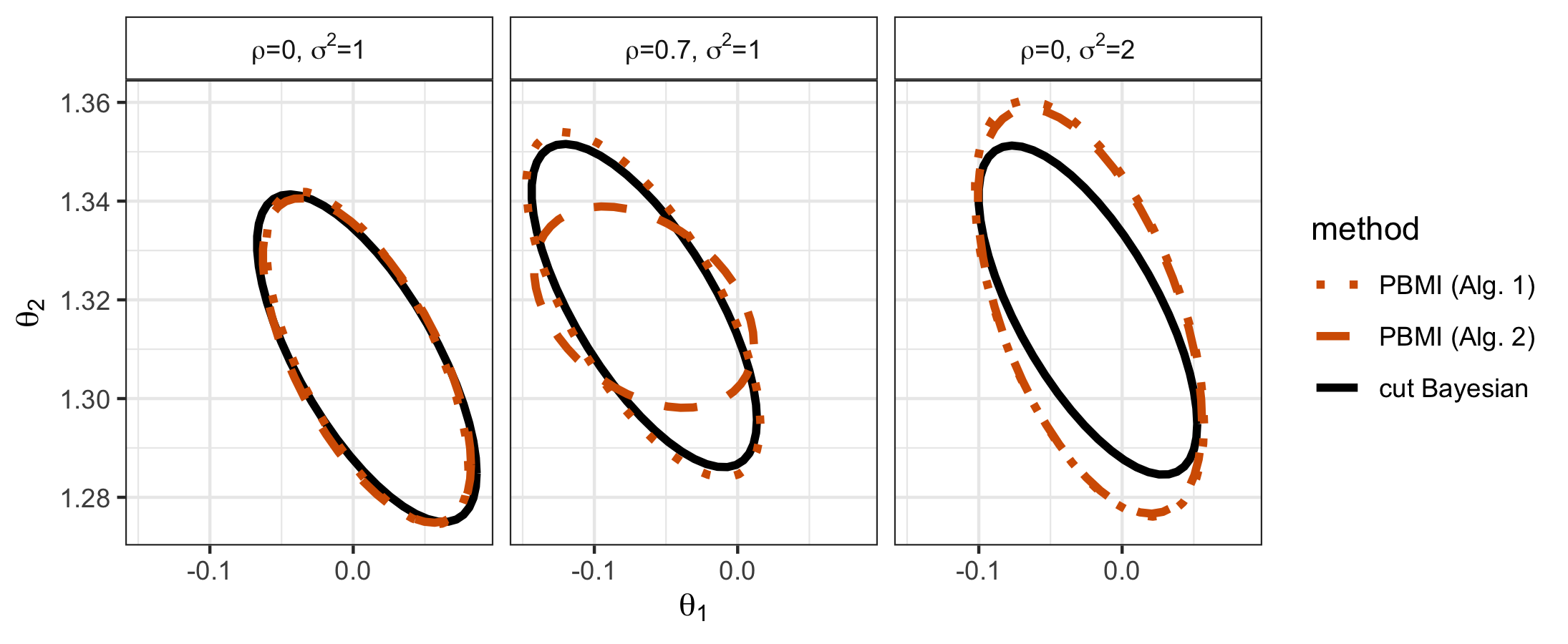
Figure 1: Density contours, corresponding to the 95% mass region, for samples obtained using PBMI (Algorithm 1 and Algorithm 2) and Bayesian modular inference for model (18). We considered three settings, depending on the choice of $\rho$ and $\sigma^{2}$ in the data-generating mechanism. Each plot is based on $N=2000$ samples.

We consider the following model:

$$\begin{split}z_{i}&\sim N(\theta_{1},1),\quad i=1,\ldots,n\\ y_{i}&\sim N(\theta_{1}+\theta_{2}x_{i},1),\quad i=1,\ldots,n.\end{split}$$ (18)

Independent $N(0,10^{2})$ priors are set on $\theta_{1}$ and $\theta_{2}$. We generate $x_{1},\ldots,x_{n}\sim N(3,1)$ with $n=800$. The observations $(z_{i},y_{i})$ are generated from the bivariate Normal distribution with mean $(0,1+x_{i})$ and covariance matrix

$$\begin{pmatrix}1&\rho\\ \rho&\sigma^{2}\end{pmatrix}.$$

We consider three different settings, depending on the values of $\rho$ and $\sigma^{2}$. Note that setting $\rho=0$ makes $z_{i}$ and $y_{i}$ independent, as in Scenario 1; setting $\sigma^{2}\neq 1$ makes the second module misspecified.

Figure 1 presents results for these three settings, under Bayesian modular inference and under PBMI. Since both modules have the same number of observations, in case of PBMI we used both Algorithm 1 and Algorithm 2 in order to compare the results. In the first scenario, depicted in the leftmost panel, both modules are well-specified and there is no dependence between datasets $z_{1},\ldots,z_{n}$ and $y_{1},\ldots,y_{n}$. As expected from Proposition 3 and Theorems 1 and 2, all three methods provide very similar results. Note that the distributions on $\theta_{2}$ are located around $4/3$, since the distribution on $\theta_{1}$ is located around zero, and since $y_{i}$ is centered around $4$ and $x_{i}$ around $3$.

The middle panel illustrates a situation when both modules separately are well-specified, while the whole model is misspecified, as it does not represent correctly the correlation between the error terms. We notice that the cut posterior fails to account for correlation between the considered likelihoods, and so does Algorithm 1. Algorithm 2 has the capacity to adjust for it, thanks to the use of the same weights at both sampling stages. The rightmost panel shows that Posterior Bootstrap corrects the uncertainty when the second module is misspecified.

4.2 Biased data

We revisit the biased data example of Liu et al. [2009], introduced in Section 2.1:

$$\begin{split}x_{1,i}&\sim N(\theta_{1},1),\quad i=1,\ldots,n_{1},\\ x_{2,i}&\sim N(\theta_{1}+\theta_{2},1),\quad i=1,\ldots,n_{2}.\end{split}$$ (19)

The priors for $\theta_{1}$ and $\theta_{2}$ are independent $N(0,1)$ and $N(0,0.1^{2})$. The data $x_{1,1:n_{1}}$ and $x_{2:1:n_{2}}$ is generated independently, from distributions $N(0,\sigma_{1}^{2})$ and $N(1,\sigma_{2}^{2})$, respectively. Thus the magnitude of the “bias” parameter $\theta_{2}$ is poorly anticipated a priori. In what follows we consider different settings, depending on the values of $\sigma_{1}^{2},\sigma_{2}^{2},n_{1}$ and $n_{2}$.

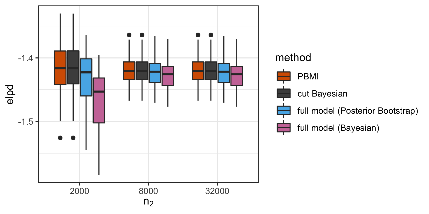
Figure 2: Boxplots of elpd values obtained for model (19). Each plot is based on 50 datasets generated with $\sigma_{1}^{2}=1$, $\sigma_{2}^{2}=0.5$, $n_{2}$ presented on the $x$-axis and $n_{1}=n_{2}/10$. We use $N=2000$ samples drawn using each method.

Here we assume that the interest lies in the prediction using the first module, that is, prediction on $x_{1,n_{1}+1}$. To this end we empirically measured the expected log pointwise predictive density for a new dataset (elpd) [Bernardo and Smith, 2009, Gneiting and Raftery, 2007, Vehtari et al., 2017]. Recall that, using notation from model (5), and denoting the new dataset by $\tilde{x}_{1},\ldots,\tilde{x}_{n}$, elpd is defined as

$$\text{elpd}=\sum_{i=1}^{n}\int p^{*}(\tilde{x}_{i})\log\hat{p}(\tilde{x}_{i}|x_{1:n})\textrm{d}\tilde{x}_{i},$$ (20)

where $\hat{p}$ is the predictive distribution under a given method of inference.

We used four different methods: PBMI (Algorithm 1), cut posterior, joint model using Bayesian inference and joint model with Posterior Bootstrap. We set $\sigma_{1}^{2}=1$ and $\sigma_{2}^{2}=0.5$, and considered different values of $n_{2}$ while keeping $n_{1}/n_{2}=1/10$. The results are presented in Figure 2. We notice that Posterior Bootstrap outperforms Bayesian inference on the full model yielding higher elpd, the best results are however achieved by PBMI and cut posteriors. We do not observe a significant difference between the latter two because the first module is well-specified.

The fact that the prior on $\theta_{2}$ is strongly informative motivates also an analysis of the choice of hyperparameter $v_{0}$. Moreover, the interpretation of $(\theta_{1},\theta_{2})$ does not change depending on $\sigma_{1}^{2}$ and $\sigma_{2}^{2}$, so it is justified to compare our samples drawn from PBMI to results obtained using the cut posterior for the correct model,

$$\begin{split}x_{1,i}&\sim N(\theta_{1},\sigma_{1}^{2}),\quad i=1,\ldots,n_{1},\\ x_{2,i}&\sim N(\theta_{1}+\theta_{2},\sigma_{2}^{2}),\quad i=1,\ldots,n_{2}.\end{split}$$ (21)

According to formula (17) we should set $w_{0}=\sigma_{1}^{2}$ and $v_{0}=\sigma_{2}^{2}$. In order to check empirically which value of $v_{0}$ yields results closest to the ones obtained with a Bayesian modular approach with the correct distribution (21), we measured Kolmogorov–Smirnov dissimilarity between samples $\theta_{2}$ from the cut posterior for the correct model (21) and samples obtained using PBMI (see Figure 3). Recall that Kolmogorov–Smirnov dissimilarity measures the maximum distance between two empirical cumulative distribution functions. The plots in Figure 3 confirm that setting $v_{0}$ according to formula (17) yields the best performance on this example.

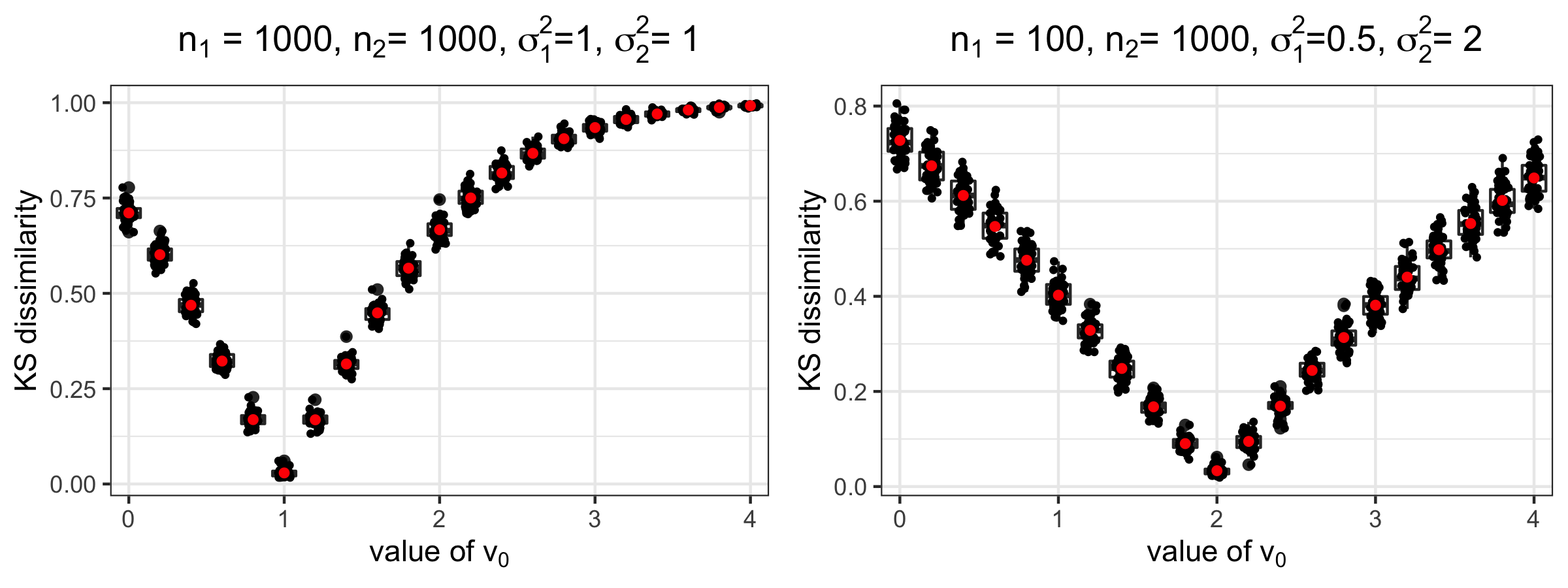
Figure 3: Kolmogorov–Smirnov dissimilarity between samples $\theta_{2}$ from the cut posterior for the correct model (21) and samples obtained using PBMI (Algorithm 1) for model (19). We consider two different settings of $\sigma_{1}^{2},\sigma_{2}^{2},n_{1}$ and $n_{2}$. Each plot is based on 50 simulated datasets and $N=2000$ samples drawn using each method.

4.3 Causal inference with propensity scores

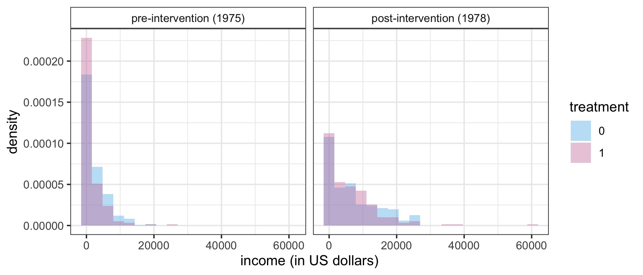
Figure 4: Histograms of income of the participants of the study, pre-intervention (left panel) and post-intervention (right panel) for the treated and the non-treated group.

To illustrate the performance of Algorithm 2 on causal inference models described in Section 2.2, we revisit the example studied extensively by LaLonde [1986] and later by Dehejia and Wahba [1999], who measured the effect of a labour training for the post-intervention income. The dataset comes from National Supported Work Demonstration and the Population Survey of Income Dynamics, and is currently available as the lalonde dataset in MatchIt R package. The treatment assignment was not randomized, in particular the assignment to the intervention was highly dependent on the pre-intervention income (see Figure 4).

Following Dehejia and Wahba [1999], we define the first module as a logistic regression with treatment as the dependent variable, and the following covariates: age, age squared, number of years of schooling, race (black, Hispanic or white) an indicator for being married, an indicator for whether the individual has a high school degree, income in 1974 and income in 1975. We standardized all continuous variables so that they have mean 0 and variance 1. The second module is a linear regression model, where the outcome variable $Y_{i}$ is the income of individual $i$ after the intervention (in 1978), standardized to have expectation 0 and variance 1. The dependent variables are the indicator of treatment and quintiles of propensity scores, obtained in the first part of the model. To this end, we will write $\text{ps}_{i}=k$ to denote that the propensity score of individual $i$ falls into the $k$th quintile. Using the notation from Section 2.2, we can summarize this model as follows:

$$\begin{split}\text{logit}P(Z_{i}=1|X_{i})=&\beta_{1,0}+\beta_{1,1}X_{i,1}+\ldots+\beta_{1,p}X_{i,p}\\ Y_{i}=&\beta_{\text{treat}}Z_{i}+\beta_{2,0}+\sum_{k=2}^{5}\beta_{2,k}\delta_{k}(\text{ps}_{i})+\epsilon,\quad\epsilon\sim N(0,\sigma^{2}),\end{split}$$ (22)

where $\delta_{k}(\text{ps}_{i})=1$ when $\text{ps}_{i}=k$ and 0 otherwise. Since the dependent variable has many zeros, as shown in Figure 4, we suspect that the second module is misspecified.

We compare the results obtained using Bayesian modular inference with those obtained using our Algorithm 2. In case of Bayesian inference, we used vague priors for all parameters involved, that is, $\beta_{1,1},\ldots,\beta_{1,p}$ in the logistic regression in the first module, as well as parameters $\beta$ and $\sigma$ in the linear regression in the second module. In case of PBMI we set $w_{0}=v_{0}=0$. The parameter of particular interest is $\beta_{\text{treat}}$, depicted in Figure 5. We notice that PBMI yields more narrow credible intervals around the mean, suggesting that the intervention had a positive impact on the income with increased certainty.

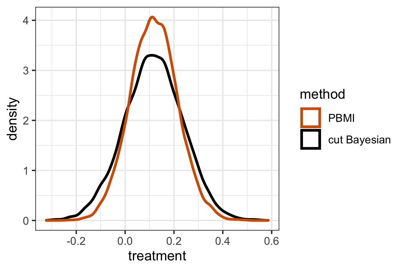
Figure 5: Density plot of $\beta_{\text{treat}}$ drawn from the cut posterior under model (22), and from Algorithm 2. Each plot is based on $N=10000$ samples.

4.4 Epidemiological study

The example we present below comes originally from Maucort-Boulch et al. [2008], who investigated the international correlation between human papillomavirus (HPV) prevalence and cervical cancer incidence. It was used as an example in Plummer [2015], Jacob et al. [2017, 2020], Carmona and Nicholls [2020].

Cervical cancer is known to be caused by around 20 “high-risk” types of HPV. This epidemiological study considers two modules, based on two different data sources. The high-risk HPV prevalence dataset was obtained via a series of surveys carried out in 13 different countries. Incidence data come from cancer registries in the same populations. In each population $i$, for $i=1,\ldots,13$, we let $Z_{i}$ be the number of women infected with high-risk HPV in a sample of size $n_{1,i}$ from the same population. Moreover, the outcome $Y_{i}$ denotes the number of cancer cases arising from $T_{i}$ woman-years of follow-up. We consider the following model.

$$\begin{split}Z_{i}\sim&\text{Binomial}(n_{1,i},\theta_{1,i})\\ \log\mu_{i}=&\theta_{2,1}+\theta_{2,2}\theta_{1,i}+T_{i}\\ Y_{i}\sim&\text{Poisson}(\mu_{i}).\end{split}$$ (23)

We set independent priors $\theta_{1,i}\sim\text{Beta}(1,1)$ for $i=1,\ldots,13$. The prior for $\theta_{2}$ is $\theta_{2,1}\sim N(0,10^{3})$, $\theta_{2,2}\sim N(0,10^{3})$. As mentioned by Plummer [2015], the log-linear relationship $\log\mu_{i}=\theta_{2,1}+\theta_{2,2}\theta_{1,i}+T_{i}$ is speculative, which suggests the misspecification of the second module.

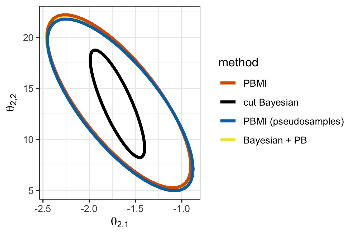
Figure 6: Density contour plots, corresponding to the 95% mass region, for $(\theta_{2,1},\theta_{2,2})$ in model (23) obtained using four different methods. We used Algorithm 1 (PBMI), PBMI where at the first stage the prior information is incorporated via pseudosamples (PBMI pseudosamples), a combination of Bayesian inference at the first stage and Posterior Bootstrap at the second stage (Bayesian+PB), and Bayesian modular inference (cut Bayesian). Each plot is based on $N=5000$ samples.

It is worth emphasizing that the small number of countries considered in this study ($n_{2}=13$) casts some doubts on whether the estimators have reached their asymptotic regime. Moreover, in this kind of studies, where the first module is based on individual-level data, whereas the second module is build around country-level data, the number of observations at the first level will be an order of magnitude larger than the number of countries. In particular, this setting does not correspond to any of the cases considered in Theorems 1 and 2.

We nevertheless applied PBMI to this example, using a slightly modified version of Algorithm 1, where at the first stage of inference we use separate Posterior Bootstrap procedures to draw $\tilde{\theta}_{1,i}$ for $i=1,\ldots,13$. We also applied to this model a version of PBMI where instead of penalization we use the pseudosamples strategy to incorporate the prior information in the first module. Note that the use of pseudosamples is justified thanks to conjugacy of the Beta prior. Finally, since we believe the first module is well-specified, and the use of conjugate priors allows for drawing directly samples from the Bayesian posterior, we combined the use of Bayesian inference for the first module with Posterior Bootstrap, given the draws of $\theta_{1,i}$, $i=1,\ldots,13$, for the second module. We compared the above approaches to the standard Bayesian modular inference. To sample from the cut posterior, we first drew directly 5000 samples from the posterior distribution for the first module, and then for each of these samples we ran a Markov chain targeting the posterior associated with the second module given $\theta_{1}$. We assumed that the burn-in period of 5000 was enough for each chain to reach stationarity.

In Figure 6 we present results obtained for $(\theta_{2,1},\theta_{2,2})$ using the four methods described above. We notice that the credible regions for the cut distribution are much smaller than the credible regions under any of the other methods. It is worth pointing out that credible regions under PBMI may be either narrower, as in Figure 6, or wider, as in Figure 5, than credible regions derived from cut posteriors.

We also calculated elpd (20) for PBMI and the cut posterior, using leave-one-out cross-validation. The results were -9.22 for the cut posterior and -6.27 for PBMI. In summary, these results suggest that Posterior Bootstrap corrects for misspecification of the second module by adjusting the uncertainty, and outperforms the cut posterior in terms of prediction.

5 Discussion

The proposal of this article participates in an emerging range of alternatives to standard Bayesian inference, designed to retain the benefits of fully probabilistic approaches while addressing the issue of model misspecification, and specifically here the setting of models built of multiple modules [Liu et al., 2009, Jacob et al., 2017, Leonelli et al., 2018, Goudie et al., 2019, Manderson and Goudie, 2020].

The main contributions of this work are two-fold. Firstly, we found the Laplace approximation of the cut posteriors and explained its lack of the appropriate frequentist coverage. As a remedy to this issue, we designed Posterior Bootstrap for Modular Inference, and proved its theoretical properties, regarding inference and prediction. In particular, we showed that its credible regions are asymptotically confidence sets in the frequentist sense. Our methodology is robust to misspecification and allows for performing the computations fully in parallel. Even though each of the module in this article was presented as a non-hierarchical model, our approach can be extended to certain types of hierarchical models, following the strategies developed by Pompe [2021]. Moreover, the methodology could be extended to more than two modules.

Our methodology inherits the limitations of Weighted Likelihood Bootstrap and Posterior Bootstrap. In particular, performing optimization typically involves computing gradients, therefore Posterior Bootstrap is not well-suited for distributions defined on discrete or mixed state spaces. Moreover, only asymptotic theory is known for methods based on Posterior Bootstrap. However, there are recent approaches looking into establishing finite sample properties of methods based on Weighted Likelihood Bootstrap [Walker, 2021].

In asymptotic regimes, an alternative to our methodology would be to obtain the Normal distributions in Propositions 1 and 2, by replacing the asymptotic covariance matrices by empirical estimates. Our approach allows the use of prior knowledge and does not require computing information matrices, but a thorough comparison of these types of approaches would be of interest, perhaps using higher-order asymptotics.

Acknowledgements

We thank Judith Rousseau and Chris Carmona for feedback and helpful discussions. EP is supported by the EPSRC and MRC Centre for Doctoral Training in Next Generation Statistical Science: the Oxford-Warwick Statistics Programme, EP/L016710/1, and the Clarendon Fund.

Appendix A Proofs of theoretical results

A.1 Assumptions

Following [Newton, 1991, Lyddon et al., 2019, Pompe, 2021] we consider the following regularity conditions. The data-generating distributions of $x_{1,1:n_{1}}$ and $x_{2,1:n_{2}}$ are denoted by $P_{1}^{*}$ and $P_{2}^{*}$.

Assumption 1.

(Log likelihood functions). The log likelihood functions $\ell_{1}(x_{1},\theta_{1})=\log f_{1}(x_{1}|\theta_{1})$ and $\ell_{2}(x_{2},\theta_{1},\theta_{2})=\log f_{2}(x_{2}|\theta_{1},\theta_{2})$ are measurable and bounded from above, with $E_{p_{1}^{*}}\big{|}\ell_{1}(X_{1},\theta_{1})\big{|}<\infty$, $E_{p_{2}^{*}}\big{|}\ell_{2}(X_{2},\theta_{1},\theta_{2})\big{|}<\infty$ for all $\theta_{1}\in\Theta_{1}$, $\theta_{2}\in\Theta_{2}$.

Assumption 2.

(Identifiability). There exists a unique maximizing parameter value

$$\theta_{1}^{*}=\arg\max_{\theta_{1}\in\Theta_{1}}\mathbb{E}_{p_{1}^{*}}\left\{\ell_{1}(X_{1},\theta_{1})\right\}.$$

Moreover, there is an open ball $B\subseteq\Theta_{1}$ containing $\theta_{1}^{*}$ such that for each $\theta_{1}\in B$ we have a unique maximizer

$$\theta_{2}^{*}(\theta_{1})=\arg\max_{\theta_{2}\in\Theta_{2}}\mathbb{E}_{p_{2}^{*}}\left\{\ell_{2}(X_{2},\theta_{1},\theta_{2})\right\}.$$

Furthermore, for all $\delta>0$ there exists an $\epsilon>0$ such that

$$\lim_{n\to\infty}P_{1}^{*}\left[\sup_{\|\theta_{1}-\theta_{1}^{*}\|\geq\delta}\frac{1}{n}\sum_{j=1}^{n}\left\{\ell_{1}(X_{1,j},\theta)-\ell_{1}(X_{1,j},\theta_{1}^{*})\right\}\leq-\epsilon\right]=1,$$ (24)

and

$$\lim_{n\to\infty}P_{2}^{*}\left[\sup_{\|(\theta_{1}-\theta_{1}^{*},\theta_{2}-\theta_{2}^{*})\|\geq\delta}\frac{1}{n}\sum_{j=1}^{n}\left\{\ell_{2}(X_{2,j},\theta_{1},\theta_{2})-\ell_{2}(X_{2,j},\theta_{1}^{*},\theta_{2}^{*})\right\}\leq-\epsilon\right]=1.$$ (25)

Assumption 3.

(Smoothness of the log likelihood function). There is an open ball $B_{1}\subseteq\Theta_{1}$ containing $\theta_{1}^{*}$ such that $\ell_{1}(x_{1},\theta_{1})$ is three times continuously differentiable with respect to $\theta_{1}\in B_{1}$ almost surely on $x_{1}$ with respect to $P_{1}^{*}$. Moreover, there is an open ball $B_{2}\subseteq\Theta_{2}$ containing $\theta_{2}^{*}$ such that $\ell_{2}(x_{2},\theta_{1},\theta_{2})$ is three times continuously differentiable with respect to $\theta_{1}$ and $\theta_{2}$ for $(\theta_{1},\theta_{2})\in B_{1}\times B_{2}$, almost surely on $x_{2}$ with respect to $P_{2}^{*}$.

We additionally impose certain moment conditions on the partial derivatives. There exist measurable functions $G_{k}$ for $k=1,\ldots,6$ such that for $(\theta_{1},\theta_{2})\in B_{1}\times B_{2}$ we have

$$\Big{|}\frac{\partial\ell_{1}(x_{1},\theta_{1})}{\partial\theta_{j}}\Big{|} \leq G_{1}(x_{1}), 1\leq j\leq d_{1}, \mathbb{E}_{p_{1}*}\left\{G_{1}(X_{1})^{4}\right\} <\infty,$$

$$\Big{|}\frac{\partial^{2}\ell_{1}(x_{1},\theta_{1})}{\partial\theta_{j}\partial\theta_{k}}\Big{|} \leq G_{2}(x_{1}), 1\leq j\leq k\leq d_{1}, \mathbb{E}_{p_{1}*}\left\{G_{2}(X_{1})^{4}\right\} <\infty,$$

$$\Big{|}\frac{\partial^{3}\ell_{1}(x_{1},\theta_{1})}{\partial\theta_{j}\partial\theta_{k}\partial\theta_{l}}\Big{|} \leq G_{3}(x_{1}), 1\leq j\leq k\leq l\leq d_{1} \mathbb{E}_{p_{1}*}\left\{G_{3}(X_{1})\right\} <\infty$$

$$\Big{|}\frac{\partial\ell_{2}(x_{2},\theta_{1},\theta_{2})}{\partial\theta_{j}}\Big{|} \leq G_{4}(x_{2}), 1\leq j\leq(d_{1}+d_{2}), \mathbb{E}_{p_{2}*}\left\{G_{1}(X_{2})^{4}\right\} <\infty,$$

$$\Big{|}\frac{\partial^{2}\ell_{2}(x_{2},\theta_{1},\theta_{2})}{\partial\theta_{j}\partial\theta_{k}}\Big{|} \leq G_{5}(x_{2}), 1\leq j\leq k\leq(d_{1}+d_{2}), \mathbb{E}_{p_{2}*}\left\{G_{5}(X_{2})^{4}\right\} <\infty,$$

$$\Big{|}\frac{\partial^{3}\ell_{2}(x_{2},\theta_{1},\theta_{2})}{\partial\theta_{j}\partial\theta_{k}\partial\theta_{l}}\Big{|} \leq G_{6}(x_{2}), 1\leq j\leq k\leq l\leq(d_{1}+d_{2}), \mathbb{E}_{p_{2}*}\left\{G_{6}(X_{2})\right\} <\infty,$$

where in the above equations $\theta_{m}$, $m=1,\ldots,d_{1}+d_{2}$, denotes the $m$-th coordinate of vector $\theta=(\theta_{1},\theta_{2})$.

Assumption 4.

(Positive definiteness of information matrices and linear independence of partial derivatives). For $B_{i}$ like in Assumption 3, $i=1,2$, the matrices $I_{i}$ and $J_{i}$ defined as

$$I_{1}(\theta_{1})= \mathbb{E}_{p_{1}^{*}}\left\{\frac{\partial\ell_{1}(X_{1},\theta_{1})}{\partial\theta_{1}}\left(\frac{\partial\ell_{1}(X_{1},\theta_{1})}{\partial\theta_{1}}\right)^{T}\right\}, J_{1}(\theta_{1})= -\mathbb{E}_{p_{1}^{*}}\left\{\frac{\partial^{2}\ell_{1}(X_{1},\theta_{1})}{\partial\theta_{1}\partial\theta_{1}^{T}}\right\},$$

$$I_{2}(\theta_{1},\theta_{2})= \mathbb{E}_{p_{2}^{*}}\left\{\frac{\partial\ell_{2}(X_{2},\theta_{1},\theta_{2})}{\partial\theta_{2}}\left(\frac{\partial\ell_{2}(X_{2},\theta_{1},\theta_{2})}{\partial\theta_{2}}\right)^{T}\right\}, J_{2}(\theta_{1},\theta_{2})= -\mathbb{E}_{p_{2}^{*}}\left\{\frac{\partial^{2}\ell_{2}(X_{2},\theta_{1},\theta_{2})}{\partial\theta_{2}\partial\theta_{2}^{T}}\right\},$$

are positive definite for $\theta_{i}\in B_{i}$ with all elements finite.

Assumption 5.

(Smoothness of log prior density). For $i=1,2$ the function $\log\pi_{i}(\theta_{i})$ is measurable, upper-bounded on $\Theta_{i}$, and three times continuously differentiable at $\theta_{i}^{*}$.

We note that (24) implies that $\hat{\theta}_{1}$ converges to $\theta_{1}^{*}$, like in standard asymptotic analysis for one module. To show that $\hat{\theta}_{2}$ converges to $\theta_{2}^{*}$, we notice that

$$\frac{1}{n}\sum_{j=1}^{n}\left\{\ell_{2}(X_{2,j},\hat{\theta}_{1},\hat{\theta}_{2})-\ell_{2}(X_{2,j},\theta_{1}^{*},\theta_{2}^{*})\right\}$$

$$= \frac{1}{n}\sum_{j=1}^{n}\left\{\ell_{2}(X_{2,j},\hat{\theta}_{1},\hat{\theta}_{2})-\ell_{2}(X_{2,j},\hat{\theta}_{1},\theta_{2}^{*})\right\}+\frac{1}{n}\sum_{j=1}^{n}\left\{\ell_{2}(X_{2,j},\hat{\theta}_{1},{\theta}_{2}^{*})-\ell_{2}(X_{2,j},{\theta}_{1}^{*},\theta_{2}^{*})\right\}.$$

Thus by equation (25), the fact that $\hat{\theta}_{1}$ converges to $\theta_{1}^{*}$, and the smoothness of $\ell_{2}$ with respect to $\theta_{1}$ in the neighbourhood of $\theta_{1}^{*}$ we infer that $\hat{\theta}_{2}$ converges to $\theta_{2}^{*}$.

To show that $(\tilde{\theta}_{1},\tilde{\theta}_{2})$ converges to $(\theta_{1}^{*},\theta_{2}^{*})$, we can therefore follow the steps of Newton [1991].

A.2 Proof of Proposition 3

Proof.

In this proof we will use the fact that, as noticed by Plummer [2015], there are two equivalent ways of defining cut posteriors. The first one relies on writing its density in the form (3). Alternatively, one can define the cut posterior for $(\theta_{1},\theta_{2})$ through its sampling scheme: we first sample $\theta_{1}$ from $\pi(\theta_{1}|x_{1,1:n_{1}})$, and then $\theta_{2}$ given $\theta_{1}$ from $\pi(\theta_{2}|x_{2,1:n_{2}},\theta_{1})$.

We will now follow standard steps to obtain the Laplace approximation of posterior densities, utilizing the Taylor expansion of the logarithm of the density; see for example Van der Vaart [2000]. Firstly, the second definition above justifies why we choose $(\hat{\theta}_{1},\hat{\theta}_{2})$ as the centring point. The assumptions listed in Section A.1 ensure that the incurred error in the Taylor expansion is small enough so that $\sqrt{n_{2}}(\theta_{1}-\hat{\theta}_{1},\theta_{1}-\hat{\theta}_{1})$ converges in distribution to a Normal distribution. It remains to find the limiting covariance matrix $\Sigma_{B}$.

We have

$$\log\pi_{\text{cut}}(\theta_{1},\theta_{2})= \sum_{j=1}^{n_{1}}\log f_{1}(x_{1,j}|\theta_{1})+\sum_{j=1}^{n_{2}}\log f_{2}(x_{2,j}|\theta_{1},\theta_{2})+\log\pi_{1}(\theta_{1})+\log\pi_{2}(\theta_{2})$$

$$\quad-\log\int\prod_{j=1}^{n_{2}}f_{2}(x_{2,j}|\theta_{1},\theta_{2})\pi_{2}(\theta_{2})d\theta_{2}.$$

We thus obtain

$$-\frac{1}{n_{2}}\frac{\partial^{2}\log\pi_{\text{cut}}(\hat{\theta}_{1},\hat{\theta}_{2})}{\partial\theta_{2}\partial\theta_{2}^{T}}=-\frac{1}{n_{2}}\sum_{j=1}^{n_{2}}\frac{\partial^{2}\log f_{2}(x_{2,j}|\hat{\theta}_{1},\hat{\theta}_{2})}{\partial\theta_{2}\partial\theta_{2}^{T}},$$

and

$$-\frac{1}{n_{2}}\frac{\partial^{2}\log\pi_{\text{cut}}(\hat{\theta}_{1},\hat{\theta}_{2})}{\partial\theta_{1}\partial\theta_{2}^{T}}=-\frac{1}{n_{2}}\sum_{j=1}^{n_{2}}\frac{\partial^{2}\log f_{2}(x_{2,j}|\hat{\theta}_{1},\hat{\theta}_{2})}{\partial\theta_{1}\partial\theta_{2}^{T}},$$

which converge in distribution to $J_{2}^{*}$ and $R_{J}$, respectively. Therefore

$$\Sigma_{B}^{-1}=\begin{pmatrix}A&R_{J}^{*}\\ R_{J}^{*T}&J_{2}^{*}\end{pmatrix}$$

for some matrix $A$. To find this matrix, we use the formula for inverting a block matrix,

$$\Sigma_{B}=\begin{pmatrix}(A-R_{J}^{*}J_{2}^{*-1}R_{J}^{T})^{-1}&-(A-R_{J}^{*}J_{2}^{*-1}R_{J}^{*T})^{-1}R_{J}^{*}J_{2}^{*-1}\\ -J_{2}^{*-1}R_{J}^{*T}(A-R_{J}^{*}J_{2}^{*-1}R_{J}^{*T})^{-1}&J_{2}^{*-1}+J_{2}^{*-1}R_{J}^{*T}(A-R_{J}^{*}J_{2}^{*-1}R_{J}^{*T})^{-1}R_{J}^{*}J_{2}^{*-1}\end{pmatrix}.$$

Recall that $\theta_{1}$ is drawn from $\pi(\theta_{1}|x_{1,1:n_{1}})$, so the limiting distribution of $\sqrt{n_{1}}(\theta_{1}-\hat{\theta}_{1})$ is $N(0,J_{1}^{*-1})$. Therefore we must have

$$(A-R_{J}^{*}J_{2}^{*-1}R_{J}^{*T})^{-1}=\frac{1}{\alpha}J_{1}^{*-1},$$

which provides the expression of $A$ and completes the proof. ∎

A.3 Proofs of Theorems 1 and 2

We first present the proof of Theorem 1. We will then use a similar reasoning to prove Theorem 2.

Proof.

Let $\ell_{1}(x_{1,j},\theta_{1})=\log f_{1}(x_{1,j}|\theta_{1})$ and $\ell_{2}(x_{2,j},\theta_{1},\theta_{2})=\log f_{2}(x_{2,j}|\theta_{1},\theta_{2})$. We also define

$$L_{1}^{w}(\theta_{1})=\sum_{j=1}^{n_{1}}w_{j}\ell_{1}(x_{1,j},\theta_{1})+w_{0}^{T}\log\pi_{1}(\theta_{1})$$

and

$$L_{2}^{v}(\theta_{1},\theta_{2})=\sum_{j=1}^{n_{2}}v_{j}\ell_{2}(x_{2,j},\theta_{1},\theta_{2})+v_{0}(\theta_{1})\log\pi_{2}(\theta_{2}).$$

Then

$$0=\frac{\partial L_{1}^{w}(\tilde{\theta}_{1})}{\partial\theta_{1}}=\frac{\partial L_{1}^{w}(\hat{\theta}_{1})}{\partial\theta_{1}}+\frac{\partial^{2}L_{1}^{w}(\hat{\theta}_{1})}{\partial\theta_{1}\partial\theta_{1}^{T}}(\tilde{\theta}_{1}-\hat{\theta}_{1})+O_{P}\left(n_{2}\|\tilde{\theta}_{1}-\hat{\theta}_{1}\|^{2}\right)$$

and therefore

$$-\frac{1}{\sqrt{n_{2}}}\frac{\partial L_{1}^{w}(\hat{\theta}_{1})}{\partial\theta_{1}}=\frac{1}{n_{2}}\frac{\partial^{2}L_{1}^{w}(\hat{\theta}_{1})}{\partial\theta_{1}\partial\theta_{1}^{T}}\sqrt{n_{2}}(\tilde{\theta}_{1}-\hat{\theta}_{1})+O_{P}\left(\sqrt{n_{2}}\|\tilde{\theta}_{1}-\hat{\theta}_{1}\|^{2}\right).$$ (26)

For the second module we have

$$0=\frac{\partial L_{2}^{v}(\tilde{\theta}_{1},\tilde{\theta}_{2})}{\partial\theta_{2}}=\frac{\partial L_{2}^{v}(\hat{\theta}_{1},\hat{\theta}_{2})}{\partial\theta_{2}}+\frac{\partial^{2}L_{2}^{v}(\hat{\theta}_{1},\hat{\theta}_{2})}{\partial\theta_{1}^{T}\partial\theta_{2}}(\tilde{\theta}_{1}-\hat{\theta}_{1})+\frac{\partial^{2}L_{2}^{v}(\hat{\theta}_{1},\hat{\theta}_{2})}{\partial\theta_{2}\partial\theta_{2}^{T}}(\tilde{\theta}_{2}-\hat{\theta}_{2})+O_{P}\left(n_{2}\|\tilde{\theta}-\hat{\theta}\|^{2}\right),$$

where $\tilde{\theta}=(\tilde{\theta}_{1},\tilde{\theta}_{2})$ and $\hat{\theta}=(\hat{\theta}_{1},\hat{\theta}_{2})$. Similarly, we have

$$-\frac{1}{\sqrt{n_{2}}}\frac{\partial L_{2}^{v}(\hat{\theta}_{1},\hat{\theta}_{2})}{\partial\theta_{2}}-\frac{1}{n_{2}}\frac{\partial^{2}L_{2}^{v}(\hat{\theta}_{1},\hat{\theta}_{2})}{\partial\theta_{1}^{T}\partial\theta_{2}}\sqrt{n_{2}}(\tilde{\theta}_{1}-\hat{\theta}_{1})=\frac{\partial^{2}L_{2}^{v}(\hat{\theta}_{1},\hat{\theta}_{2})}{\partial\theta_{2}\partial\theta_{2}^{T}}\frac{\sqrt{n_{2}}}{n_{2}}(\tilde{\theta}_{2}-\hat{\theta}_{2})+O_{P}\left(\sqrt{n_{2}}\|\tilde{\theta}-\hat{\theta}\|^{2}\right).$$ (27)

Note that

$$-\frac{1}{n_{2}}\frac{\partial^{2}L_{1}^{w}(\hat{\theta}_{1})}{\partial\theta_{1}\partial\theta_{1}^{T}},\quad-\frac{1}{n_{2}}\frac{\partial^{2}L_{2}^{v}(\hat{\theta}_{1},\hat{\theta}_{2})}{\partial\theta_{1}^{T}\partial\theta_{2}},\quad-\frac{1}{n_{2}}\frac{\partial^{2}L_{2}^{v}(\hat{\theta}_{1},\hat{\theta}_{2})}{\partial\theta_{2}\partial\theta_{2}^{T}}$$

converge in probability to $\alpha J_{1}^{*}$, $R_{J}^{*T}$ and $J_{2}^{*}$, respectively. Therefore using (26) and (27) we get that

$$\begin{split}\sqrt{n_{2}}(\tilde{\theta}_{2}-\hat{\theta}_{2})=&J_{2}^{*-1}\frac{1}{\sqrt{n_{2}}}\frac{\partial L_{2}^{v}(\hat{\theta}_{1},\hat{\theta}_{2})}{\partial\theta_{2}}-J_{2}^{*-1}R_{J}^{*T}\sqrt{n_{2}}(\tilde{\theta}_{1}-\hat{\theta}_{1})+O_{P}\left(\sqrt{n_{2}}\|\tilde{\theta}-\hat{\theta}\|^{2}\right)\\ =&J_{2}^{*-1}\frac{1}{\sqrt{n_{2}}}\frac{\partial L_{2}^{v}(\hat{\theta}_{1},\hat{\theta}_{2})}{\partial\theta_{2}}-J_{2}^{*-1}R_{J}^{*T}J_{1}^{*-1}\frac{1}{\alpha\sqrt{n_{2}}}\frac{\partial L_{1}^{w}(\hat{\theta}_{1})}{\partial\theta_{1}}+O_{P}\left(\sqrt{n_{2}}\|\tilde{\theta}-\hat{\theta}\|^{2}\right).\end{split}$$ (28)

We will now find the asymptotic distribution of

$$\left(\frac{1}{\sqrt{n_{2}}}\frac{\partial L_{1}^{w}(\hat{\theta}_{1})}{\partial\theta_{1}},\frac{1}{\sqrt{n_{2}}}\frac{\partial L_{2}^{v}(\hat{\theta}_{1},\hat{\theta}_{2})}{\partial\theta_{2}}\Big{|}x_{1,1:n_{1}},x_{2,1:n_{2}}\right).$$ (29)

Since

$$\sum_{j=1}^{n_{1}}\frac{\partial\ell_{1}(x_{1,j},\hat{\theta}_{1})}{\partial\theta_{1}}=0,\quad\sum_{j=1}^{n_{2}}\frac{\partial\ell_{2}(x_{2,j},\hat{\theta}_{1},\hat{\theta}_{2})}{\partial\theta_{2}}=0$$

we have

$$\frac{\partial L_{1}^{w}(\hat{\theta}_{1})}{\partial\theta_{1}}=\sum_{j=1}^{n_{1}}\frac{(w_{j}-1)\partial\ell_{1}(x_{1,j},\hat{\theta}_{1})}{\partial\theta_{1}}+w_{0}^{T}\frac{\partial\log\pi_{1}(\hat{\theta}_{1})}{\partial\theta_{1}}.$$

Similarly,

$$\frac{\partial L_{2}^{v}(\hat{\theta}_{1},\hat{\theta}_{2})}{\partial\theta_{2}}=\sum_{j=1}^{n_{2}}\frac{(v_{j}-1)\partial\ell_{2}(x_{2,j},\hat{\theta}_{1},\hat{\theta}_{2})}{\partial\theta_{2}}+v_{0}^{T}\frac{\partial\log\pi_{2}(\hat{\theta}_{2})}{\partial\theta_{2}}.$$

Therefore, applying the central limit theorem we get that the asymptotic distribution of (29) is Normal with mean 0 and covariance matrix

$$\begin{pmatrix}\alpha I_{1}^{*}&0\\ 0&I_{2}^{*}\end{pmatrix},$$

due to independence of $w_{1:n_{1}}$ and $v_{1:n_{2}}$. Finally, using Slutsky’s theorem, we get that the asymptotic distribution of $\sqrt{n_{2}}(\tilde{\theta}_{1}-\hat{\theta}_{1},\tilde{\theta}_{2}-\hat{\theta}_{2})$ given $x_{1,1:n_{1}},x_{2,1:n_{2}}$ is Normal with mean 0 and covariance matrix (8). ∎

In what follows we present the proof of Theorem 2.

Proof.

We let $\ell_{1}(x_{1,j},\theta_{1})=\log f_{1}(x_{1,j}|\theta_{1})$ and $\ell_{2}(x_{2,j},\theta_{1},\theta_{2})=\log f_{2}(x_{2,j}|\theta_{1},\theta_{2})$. We also define

$$L_{1}^{w}(\theta_{1})=\sum_{j=1}^{n}w_{j}\ell_{1}(x_{1,j},\theta_{1})+w_{0}^{T}\log\pi_{1}(\theta_{1})$$

and

$$L_{2}^{w}(\theta_{1},\theta_{2})=\sum_{j=1}^{n}w_{j}\ell_{2}(x_{2,j},\theta_{1},\theta_{2})+v_{0}^{T}\log\pi_{2}(\theta_{2}).$$

We can repeat the proof of Theorem 1 until (28), replacing $n_{1}$ and $n_{2}$ with $n$, and $v_{j}$ with $w_{j}$. Similarly to that proof, we have

$$\frac{\partial L_{1}^{w}(\hat{\theta}_{1})}{\partial\theta_{1}}=\sum_{j=1}^{n}\frac{(w_{j}-1)\partial\ell_{1}(x_{1,j},\hat{\theta}_{1})}{\partial\theta_{1}}+w_{0}^{T}\frac{\partial\log\pi_{1}(\hat{\theta}_{1})}{\partial\theta_{1}},$$

and

$$\frac{\partial L_{2}^{w}(\hat{\theta}_{1},\hat{\theta}_{2})}{\partial\theta_{2}}=\sum_{j=1}^{n}\frac{(w_{j}-1)\partial\ell_{2}(x_{2,j},\hat{\theta}_{1},\hat{\theta}_{2})}{\partial\theta_{2}}+v_{0}^{T}\frac{\partial\log\pi_{2}(\hat{\theta}_{2})}{\partial\theta_{2}}.$$

Therefore, applying the central limit theorem and the law of large numbers we get that the asymptotic distribution of

$$\left(\frac{1}{\sqrt{n}}\frac{\partial L_{1}^{w}(\hat{\theta}_{1})}{\partial\theta_{1}},\frac{1}{\sqrt{n}}\frac{\partial L_{2}^{w}(\hat{\theta}_{1},\hat{\theta}_{2})}{\partial\theta_{2}}\Big{|}x_{1,1:n},x_{2,1:n}\right)$$

is Normal with mean 0 and covariance matrix

$$\begin{pmatrix}I_{1}^{*}&R_{I}^{*}\\ R_{I}^{*T}&I_{2}^{*}\end{pmatrix},$$

since random variables $(w_{j}-1)$ for $j=1,\ldots,n$ are i.i.d. with expectation 0 and variance 1. This completes the proof. ∎

A.4 Prediction under Posterior Bootstrap for Modular Inference versus Bayesian modular inference

In what follows we first prove Proposition 4. We then design an example showing that each of the two approaches, Bayesian modular inference and PBMI, may yield better prediction for $x_{2,n_{2}+1}$, depending on the exact setting.

Proof.

In order to simplify the notation, we will denote in this proof $(x_{1,1:n_{1}},x_{2,1:n_{2}})$ by $x$, and $x_{2,n_{2}+1}$ by $x_{2}$. Moreover, by $p^{*}$ we will denote the density of the true underlying distribution of $x$. Analogously to (13), we define the risk associated with prediction for the second module, as

$$E_{p^{*}}\left[D_{KL}\left\{p_{2}^{*}||\hat{p}(\cdot|x)\right\}\right]=\int p^{*}(x)\left\{\int p_{2}^{*}(x_{2})\log\frac{p_{2}^{*}(x_{2})}{\hat{p}(x_{2}|x)}\mathrm{d}x_{2}\right\}\mathrm{d}x,$$

for a predictive distribution $\hat{p}$, which in our case will be either $\hat{p}_{B}$ or $\hat{p}_{PB}$. Firstly, notice that

$$E_{p^{*}}\left[D_{KL}\left\{p_{2}^{*}||\hat{p}(\cdot|x)\right\}\right]=-\int p^{*}(x)\left\{\int p_{2}^{*}(x_{2})\log{\hat{p}(x_{2}|x)}\mathrm{d}x_{2}\right\}\mathrm{d}x+c,$$ (30)

where the constant $c$ does not depend on the prediction method.

In order to find asymptotic expansions of $E_{p^{*}}\left[D_{KL}\left\{p_{2}^{*}||\hat{p}_{B}(\cdot|x)\right\}\right]$ and $E_{p^{*}}\left[D_{KL}\left\{p_{2}^{*}||\hat{p}_{PB}(\cdot|x)\right\}\right]$ up to $o(n_{2}^{-1})$, we will follow the steps of [Fushiki, 2010] and [Shimodaira, 2000]. We have

$$\hat{p}_{B}(x_{2}|x)=\int f_{2}(x_{2}|\theta_{1},\theta_{2})\pi_{\text{cut}}(\theta|x)\mathrm{d}\theta$$ (31)

and

$$\hat{p}_{PB}(x_{2}|x)=\int f_{2}(x_{2}|\theta_{1},\theta_{2})p^{PB}_{\text{cut}}(\theta|x)\mathrm{d}\theta.$$

We start by expanding asymptotically equation (31) around $(\hat{\theta}_{1},\hat{\theta}_{2})$. Setting $\theta=(\theta_{1},\theta_{2})$, we have

$$\hat{p}_{B}(x_{2}|x)= f_{2}(x_{2}|\hat{\theta}_{1},\hat{\theta}_{2})\int\pi_{\text{cut}}(\theta|x)\mathrm{d}\theta$$

$$\quad+\frac{\partial f_{2}(x_{2}|\hat{\theta}_{1},\hat{\theta}_{2})}{\partial\theta}\int(\theta-\hat{\theta})\pi_{\text{cut}}(\theta|x)\mathrm{d}\theta$$

$$\quad+\int(\theta-\hat{\theta})^{T}\frac{\partial^{2}f_{2}(x_{2}|\hat{\theta}_{1},\hat{\theta}_{2})}{\partial\theta\partial\theta^{T}}(\theta-\hat{\theta})\pi_{\text{cut}}(\theta|x)\mathrm{d}\theta+o_{P}(n_{2}^{-1})$$

$$= f_{2}(x_{2}|\hat{\theta}_{1},\hat{\theta}_{2})+\frac{\partial f_{2}(x_{2}|\hat{\theta}_{1},\hat{\theta}_{2})}{\partial\theta}\int(\theta-\hat{\theta})\pi_{\text{cut}}(\theta|x)\mathrm{d}\theta$$

$$\quad+\frac{1}{2n}\text{tr}\left\{\frac{\partial^{2}f_{2}(x_{2}|\hat{\theta}_{1},\hat{\theta}_{2})}{\partial\theta\partial\theta^{T}}\Sigma_{B}\right\}+o_{P}(n_{2}^{-1}),$$

and therefore

$$\begin{split}\hat{p}_{B}(x_{2}|x)=&f_{2}(x_{2}|\hat{\theta}_{1},\hat{\theta}_{2})\Bigg{[}1+\frac{\partial\log f_{2}(x_{2}|\hat{\theta}_{1},\hat{\theta}_{2})}{\partial\theta}\int(\theta-\hat{\theta})\pi_{\text{cut}}(\theta_{1},\theta_{2}|x)\mathrm{d}\theta_{1}\mathrm{d}\theta_{2}\\ &+\quad\frac{1}{2n}\text{tr}\left\{\frac{1}{f_{2}(x_{2}|\hat{\theta}_{1},\hat{\theta}_{2})}\frac{\partial^{2}f_{2}(x_{2}|\hat{\theta}_{1},\hat{\theta}_{2})}{\partial\theta\partial\theta^{T}}\Sigma_{B}\right\}\Bigg{]}+o_{P}(n_{2}^{-1}).\end{split}$$

Following Shimodaira [2000], we will use the identity

$$\frac{1}{g}\frac{\partial^{2}g}{\partial\theta\partial\theta^{T}}=\frac{\partial\log g}{\partial\theta}\frac{\partial\log g}{\partial\theta^{T}}+\frac{\partial^{2}\log g}{\partial\theta\partial\theta^{T}}.$$

Applying this identity, and the Taylor expansion of $\log(1+y)$ around $y=0$, we get

$$\begin{split}\log\hat{p}_{B}(x_{2}|x)=&\log f_{2}(x_{2}|\hat{\theta}_{1},\hat{\theta}_{2})+\frac{\partial\log f_{2}(x_{2}|\hat{\theta}_{1},\hat{\theta}_{2})}{\partial\theta}\int(\theta-\hat{\theta})\pi_{\text{cut}}(\theta_{1},\theta_{2}|x)\mathrm{d}\theta_{1}\mathrm{d}\theta_{2}\\ &+\quad\frac{1}{2n_{2}}\text{tr}\left[\left\{I_{f_{2}}^{\hat{\theta}}(x_{2})-J_{f_{2}}^{\hat{\theta}}(x_{2})\right\}\Sigma_{B}\right]+o_{P}(n_{2}^{-1}),\end{split}$$

where

$$I_{f_{2}}^{\theta}(x_{2})=\frac{\partial\log f_{2}(x_{2}|\theta_{1},\theta_{2})}{\partial\theta}\left(\frac{\partial\log f_{2}(x_{2}|\theta_{1},\theta_{2})}{\partial\theta}\right)^{T},\quad J_{f_{2}}^{\theta}(x_{2})=-\frac{\partial^{2}\log f_{2}(x_{2}|\theta_{1},\theta_{2})}{\partial\theta\partial\theta^{T}}.$$

Finally, we use equality (30) to get that

$${E}_{p^{*}}\left[D_{KL}\left\{p_{2}^{*}||\hat{p}_{B}(\cdot|x)\right\}\right]= E_{p^{*}}\left[D_{KL}\left\{p_{2}^{*}||f_{2}(\cdot|\hat{\theta}_{1},\hat{\theta}_{2})\right\}\right]-{E}_{p_{2}^{*}}\left\{\frac{\partial\log f_{2}(x_{2}|{\theta}_{1}^{*},{\theta}_{2}^{*})}{\partial\theta}\right\}\frac{a_{B}}{n_{2}}$$

$$\quad-\frac{1}{2n_{2}}\text{tr}\left\{\left(I_{f_{2}}^{*}-J_{f_{2}}^{*}\right)\Sigma_{B}\right\}+o(n_{2}^{-1}),$$

for matrices $I_{f_{2}}^{*}$ and $J_{f_{2}}^{*}$ defined in (14). Performing analogous calculations for Posterior Bootstrap, we obtain

$${E}_{p^{*}}\left[D_{KL}\left\{p_{2}^{*}||\hat{p}_{PB}(\cdot|x)\right\}\right]= E_{p^{*}}\left[D_{KL}\left\{p_{2}^{*}||f_{2}(\cdot|\hat{\theta}_{1},\hat{\theta}_{2})\right\}\right]-{E}_{p_{2}^{*}}\left\{\frac{\partial\log f_{2}(x_{2}|{\theta}_{1}^{*},{\theta}_{2}^{*})}{\partial\theta}\right\}\frac{a_{PB}}{n_{2}}$$

$$\quad-\frac{1}{2n_{2}}\text{tr}\left\{\left(I_{f_{2}}^{*}-J_{f_{2}}^{*}\right\}\Sigma_{PB}\right)+o(n_{2}^{-1}),$$

which completes the proof. ∎

As mentioned earlier, we will now use the above expansions to show that Posterior Bootstrap in some settings yields asymptotically better prediction for the second module, whereas in other settings Bayesian modular inference performs better. Let us consider the following misspecified model:

$$\begin{split}x_{1,1:n}&\sim N(\theta_{1},1),\quad\theta_{1}\sim N(0,1),\\ x_{2,1:n}&\sim N\left((\theta_{1},\theta_{2}),\Sigma_{1}\right),\quad\theta_{2}\sim N(0,1),\end{split}$$ (32)

where

$$\Sigma_{1}=\begin{pmatrix}4/3&-2/3\\ -2/3&4/3\end{pmatrix}\quad\text{and therefore}\quad\Sigma_{1}^{-1}=\begin{pmatrix}1&0.5\\ 0.5&1\end{pmatrix}.$$

In fact the data are generated independently according to

$$\begin{split}x_{1,1:n}\sim N(0,\sigma^{2}),\quad x_{2,1:n}\sim N(0,\Sigma_{2})\end{split}$$ (33)

where

$$\Sigma_{2}=\Sigma_{1}\begin{pmatrix}0.8&0.3\\ 0.3&0.8\end{pmatrix}\Sigma_{1}.$$

We consider below different scenarios for the value of $\sigma$.

Firstly, note that $(\theta_{1}^{*},\theta_{2}^{*})=(0,0)$, and that the pseudo-true parameter for $\theta_{1}$ with respect to $f_{2}$ is also equal to 0, thus

$$E_{p_{2}^{*}}\left\{\frac{\partial\log f_{2}(x_{2}|{\theta}_{1}^{*},{\theta}_{2}^{*})}{\partial\theta}\right\}=0.$$

Consequently

$$E_{p^{*}}\left[D_{KL}\left\{p_{2}^{*}||\hat{p}_{PB}(\cdot|x)\right\}\right]-E_{p^{*}}\left[D_{KL}\left\{p_{2}^{*}||\hat{p}_{B}(\cdot|x)\right\}\right]$$

$$= \frac{1}{2n}\text{tr}\left\{\left(I_{f_{2}}^{*}-J_{f_{2}}^{*}\right)\left(\Sigma_{B}-\Sigma_{PB}\right)\right\}+o(n^{-1}).$$

For this example we have

$$I_{f_{2}}^{*}=\begin{pmatrix}0.8&0.3\\ 0.3&0.8\end{pmatrix},\quad J_{f_{2}}^{*}=\begin{pmatrix}1&0.5\\ 0.5&1\end{pmatrix}$$

and $R_{J}^{*}=0.5$. Thus $J_{1}^{*-1}=1$, $J_{2}^{*-1}=1$, $I_{1}^{*}=\sigma^{2}$ and $I_{1}^{*}=2.5$. We also have

$$\Sigma_{B}=\begin{pmatrix}1&-0.5\\ -0.5&1.25\end{pmatrix},\quad\Sigma_{PB}=\begin{pmatrix}\sigma^{2}&-0.5\sigma^{2}\\ -0.5\sigma^{2}&0.8+0.25\sigma^{2}.\end{pmatrix}$$

Since

$$I_{f_{2}}^{*}-J_{f_{2}}^{*}=\begin{pmatrix}-0.2&-0.2\\ -0.2&-0.2\end{pmatrix},$$

we have $\text{tr}\{(I_{f_{2}}^{\theta^{*}}-J_{f_{2}}^{\theta^{*}})\Sigma_{B}\}=-0.25$. As for the corresponding trace for prediction based on Posterior Bootstrap, for $\sigma=1$ we have $\text{tr}\{(I_{f_{2}}^{\theta^{*}}-J_{f_{2}}^{\theta^{*}})\Sigma_{PB}\}=-0.21$, whereas for $\sigma=2$ the value of the trace is -0.36.

To summarize, we have shown that Algorithm 1 in model (32) does not necessarily yield asymptotically better prediction for the second module than Bayesian inference, and that it depends on the value of $\sigma^{2}$ in the data-generating mechanism (33).

References

- Antonelli et al. [2020] J. Antonelli, G. Papadogeorgou, and F. Dominici. Causal Inference in high dimensions: A marriage between Bayesian modeling and good frequentist properties. Biometrics, 2020.
- Bernardo and Smith [2009] J. M. Bernardo and A. F. Smith. Bayesian theory, volume 405. John Wiley & Sons, 2009.
- Bissiri et al. [2016] P. G. Bissiri, C. C. Holmes, and S. G. Walker. A general framework for updating belief distributions. Journal of the Royal Statistical Society: Series B (Statistical Methodology), 78(5):1103–1130, 2016.
- Blangiardo et al. [2011] M. Blangiardo, A. Hansell, and S. Richardson. A Bayesian model of time activity data to investigate health effect of air pollution in time series studies. Atmospheric Environment, 45(2):379–386, 2011.
- Bonvini and Kennedy [2021] M. Bonvini and E. H. Kennedy. Sensitivity analysis via the proportion of unmeasured confounding. Journal of the American Statistical Association, pages 1–11, 2021.
- Carmona and Nicholls [2020] C. Carmona and G. Nicholls. Semi-Modular Inference: enhanced learning in multi-modular models by tempering the influence of components. In International Conference on Artificial Intelligence and Statistics, pages 4226–4235. PMLR, 2020.
- Dehejia and Wahba [1999] R. H. Dehejia and S. Wahba. Causal effects in nonexperimental studies: Reevaluating the evaluation of training programs. Journal of the American statistical Association, 94(448):1053–1062, 1999.
- Fong et al. [2019] E. Fong, S. Lyddon, and C. Holmes. Scalable nonparametric sampling from multimodal posteriors with the posterior bootstrap. In International Conference on Machine Learning, pages 1952–1962. PMLR, 2019.
- Fushiki [2005] T. Fushiki. Bootstrap prediction and Bayesian prediction under misspecified models. Bernoulli, 11(4):747–758, 2005.
- Fushiki [2010] T. Fushiki. Bayesian bootstrap prediction. Journal of statistical planning and inference, 140(1):65–74, 2010.
- Gneiting and Raftery [2007] T. Gneiting and A. E. Raftery. Strictly proper scoring rules, prediction, and estimation. Journal of the American statistical Association, 102(477):359–378, 2007.
- Goudie et al. [2019] R. J. Goudie, A. M. Presanis, D. Lunn, D. De Angelis, and L. Wernisch. Joining and splitting models with Markov melding. Bayesian analysis, 14(1):81, 2019.
- Grünwald [2012] P. Grünwald. The Safe Bayesian. In International Conference on Algorithmic Learning Theory, pages 169–183. Springer, 2012.
- Grünwald and van Ommen [2017] P. Grünwald and T. van Ommen. Inconsistency of Bayesian inference for misspecified linear models, and a proposal for repairing it. Bayesian Analysis, 12(4):1069–1103, 2017.
- Hirano and Imbens [2004] K. Hirano and G. W. Imbens. The propensity score with continuous treatments. Applied Bayesian modeling and causal inference from incomplete-data perspectives, 226164:73–84, 2004.
- Huggins and Miller [2019] J. H. Huggins and J. W. Miller. Robust inference and model criticism using bagged posteriors. arXiv preprint arXiv:1912.07104, 2019.
- Huggins and Miller [2020] J. H. Huggins and J. W. Miller. Robust and reproducible model selection using bagged posteriors. arXiv preprint arXiv:2007.14845, 2020.
- Imai and Van Dyk [2004] K. Imai and D. A. Van Dyk. Causal inference with general treatment regimes: Generalizing the propensity score. Journal of the American Statistical Association, 99(467):854–866, 2004.
- Jacob et al. [2017] P. E. Jacob, L. M. Murray, C. C. Holmes, and C. P. Robert. Better together? Statistical learning in models made of modules. arXiv preprint arXiv:1708.08719, 2017.
- Jacob et al. [2020] P. E. Jacob, J. O’Leary, and Y. F. Atchadé. Unbiased Markov chain Monte Carlo methods with couplings. Journal of the Royal Statistical Society: Series B (Statistical Methodology), 82(3):543–600, 2020.
- Kleijn and Van der Vaart [2012] B. J. K. Kleijn and A. W. Van der Vaart. The Bernstein-von-Mises theorem under misspecification. Electronic Journal of Statistics, 6:354–381, 2012.
- LaLonde [1986] R. J. LaLonde. Evaluating the econometric evaluations of training programs with experimental data. The American economic review, pages 604–620, 1986.
- Leonelli et al. [2018] M. Leonelli, M. J. Barons, and J. Q. Smith. A conditional independence framework for coherent modularized inference. arXiv preprint arXiv:1807.10628, 2018.
- Little [1992] R. J. Little. Regression with missing X’s: a review. Journal of the American Statistical Association, 87(420):1227–1237, 1992.
- Liu et al. [2009] F. Liu, M. Bayarri, and J. Berger. Modularization in Bayesian analysis, with emphasis on analysis of computer models. Bayesian Analysis, 4(1):119–150, 2009.
- Liu and Goudie [2020] Y. Liu and R. J. Goudie. Stochastic Approximation Cut Algorithm for Inference in Modularized Bayesian Models. arXiv preprint arXiv:2006.01584, 2020.
- Lunn et al. [2009] D. Lunn, N. Best, D. Spiegelhalter, G. Graham, and B. Neuenschwander. Combining MCMC with ‘sequential’PKPD modelling. Journal of Pharmacokinetics and Pharmacodynamics, 36(1):19–38, 2009.
- Lyddon et al. [2018] S. Lyddon, S. Walker, and C. C. Holmes. Nonparametric learning from Bayesian models with randomized objective functions. In Advances in Neural Information Processing Systems, pages 2071–2081, 2018.
- Lyddon et al. [2019] S. Lyddon, C. Holmes, and S. Walker. General Bayesian updating and the loss-likelihood bootstrap. Biometrika, 106(2):465–478, 2019.
- Manderson and Goudie [2020] A. A. Manderson and R. J. Goudie. A numerically stable algorithm for integrating Bayesian models using Markov melding. arXiv preprint arXiv:2001.08038, 2020.
- Maucort-Boulch et al. [2008] D. Maucort-Boulch, S. Franceschi, and M. Plummer. International correlation between human papillomavirus prevalence and cervical cancer incidence. Cancer Epidemiology and Prevention Biomarkers, 17(3):717–720, 2008.
- McCandless et al. [2012] L. C. McCandless, S. Richardson, and N. Best. Adjustment for missing confounders using external validation data and propensity scores. Journal of the American Statistical Association, 107(497):40–51, 2012.
- Murphy and Topel [2002] K. M. Murphy and R. H. Topel. Estimation and inference in two-step econometric models. Journal of Business & Economic Statistics, 20(1):88–97, 2002.
- Newton [1991] M. A. Newton. The weighted likelihood bootstrap and an algorithm for prepivoting. PhD thesis, University of Washington, 1991.
- Newton and Raftery [1994] M. A. Newton and A. E. Raftery. Approximate Bayesian inference with the weighted likelihood bootstrap. Journal of the Royal Statistical Society: Series B (Methodological), 56(1):3–26, 1994.
- Newton et al. [2020] M. A. Newton, N. G. Polson, and J. Xu. Weighted Bayesian bootstrap for scalable posterior distributions. Canadian Journal of Statistics, 2020.
- Nie and Ročková [2020] L. Nie and V. Ročková. Bayesian Bootstrap Spike-and-Slab LASSO. arXiv preprint arXiv:2011.14279, 2020.
- Plummer [2015] M. Plummer. Cuts in Bayesian graphical models. Statistics and Computing, 25(1):37–43, 2015.
- Pompe [2021] E. Pompe. Introducing prior information in Weighted Likelihood Bootstrap with applications to model misspecification. arXiv preprint arXiv:2103.14445, 2021.
- Rosenbaum and Rubin [1983] P. R. Rosenbaum and D. B. Rubin. The central role of the propensity score in observational studies for causal effects. Biometrika, 70(1):41–55, 1983.
- Rubin [2004] D. B. Rubin. Multiple imputation for nonresponse in surveys, volume 81. John Wiley & Sons, 2004.
- Shimodaira [2000] H. Shimodaira. Improving predictive inference under covariate shift by weighting the log-likelihood function. Journal of statistical planning and inference, 90(2):227–244, 2000.
- Spiegelhalter et al. [2007] D. Spiegelhalter, A. Thomas, N. Best, and D. Lunn. OpenBUGS user manual. Version, 3(2):2007, 2007.
- Van der Vaart [2000] A. W. Van der Vaart. Asymptotic statistics, volume 3. Cambridge university press, 2000.
- Vehtari et al. [2017] A. Vehtari, A. Gelman, and J. Gabry. Practical Bayesian model evaluation using leave-one-out cross-validation and WAIC. Statistics and computing, 27(5):1413–1432, 2017.
- Walker [2021] S. G. Walker. On an Asymptotic Distribution for the MLE. arXiv preprint arXiv:2106.06597, 2021.
- Yu et al. [2021] X. Yu, D. J. Nott, and M. S. Smith. Variational inference for cutting feedback in misspecified models. arXiv preprint arXiv:2108.11066, 2021.
- Zellner [1988] A. Zellner. Optimal information processing and Bayes’s theorem. The American Statistician, 42(4):278–280, 1988.
- Zhang et al. [2003a] L. Zhang, S. L. Beal, and L. B. Sheiner. Simultaneous vs. sequential analysis for population PK/PD data I: best-case performance. Journal of pharmacokinetics and pharmacodynamics, 30(6):387–404, 2003a.
- Zhang et al. [2003b] L. Zhang, S. L. Beal, and L. B. Sheiner. Simultaneous vs. sequential analysis for population PK/PD data II: robustness of methods. Journal of pharmacokinetics and pharmacodynamics, 30(6):405–416, 2003b.
- Zhou and Reiter [2010] X. Zhou and J. P. Reiter. A note on Bayesian inference after multiple imputation. The American Statistician, 64(2):159–163, 2010.
- Zigler [2016] C. M. Zigler. The Central Role of Bayes’ Theorem for Joint Estimation of Causal Effects and Propensity Scores. The American Statistician, 70(1):47–54, 2016.
- Zigler et al. [2013] C. M. Zigler, K. Watts, R. W. Yeh, Y. Wang, B. A. Coull, and F. Dominici. Model feedback in Bayesian propensity score estimation. Biometrics, 69(1):263–273, 2013.