Interactions of the doubly charmed state $T_{cc}^{+}$ with a hadronic medium

Abstract

We investigate the absorption and production processes of this new state in a hadronic medium, considering the reactions $T_{cc}^{+}\pi,T_{cc}^{+}\rho\rightarrow D^{(*)}D^{(*)}$ and the corresponding inverse reactions. We use effective field Lagrangians to account for the couplings between light and heavy mesons, and give special attention to the form factors in the vertices. We calculate here for the first time the $T_{cc}^{+}-D-D^{*}$ form factor derived from QCD sum rules. The results are also obtained by testing widely utilized empirical form factors. The absorption cross sections are found to be larger than the production ones. We compare our results with the only existing estimate of these quantities, presented in a work of J. Hong, S. Cho, T. Song and S. H. Lee, in which the authors employed the quasi-free approximation. We find cross sections which are one order of magnitude smaller.

I Introduction

Very recenlty the LHCb collaboration has reported the observation of a narrow peak in the $D^{0}D^{0}\pi^{+}$-mass spectrum in proton-proton $(pp)$ collisions with statistical significance of more than $10\,\sigma$ LHCb:2021vvq ; LHCb:2021auc . By using an amplitude model based on the Breit-Wigner formalism, this peak has been fitted to one resonance with a mass of approximately $3875\mbox{ MeV}$ and quantum numbers $J^{P}=1^{+}$. Its minimum valence quark content is $cc\bar{u}\bar{d}$, giving it the unequivocal status of the first observed unconventional hadron with two heavy quarks of the same flavor. According to the data, its binding energy with respect to the $D^{*+}D^{0}$ mass threshold is $273\pm 61\pm 5_{-14}^{+11}$ keV and the decay width is $410\pm 165\pm 43_{-38}^{+18}$ keV. These values are consistent with the expected properties for a $T_{cc}^{+}$ isoscalar tetraquark ground state with $J^{P}=1^{+}$.

Even before the experimental discovery of this doubly charmed tetraquark state, there was a debate concerning its fundamental aspects, such as its decay/formation mechanisms and underlying structure  Gelman:2002wf ; Janc:2004qn ; Vijande:2003ki ; Navarra:2007yw ; Vijande:2007rf ; Ebert:2007rn ; Lee:2009rt ; Yang:2009zzp ; Hong:2018mpk ; Hudspith:2020tdf ; Cheng:2020wxa ; Qin:2020zlg . Its discovery obviously stimulated the appearance of more studies employing different theoretical approaches Agaev:2021vur ; Dong:2021bvy ; Agaev:2021vur ; Dong:2021bvy ; Huang:2021urd ; Li:2021zbw ; Ren:2021dsi ; Xin:2021wcr ; Yang:2021zhe ; Meng:2021jnw ; Ling:2021bir ; Fleming:2021wmk ; Jin:2021cxj ; Azizi:2021aib ; Hu:2021gdg . In particular, several works have investigated the implications of the $T_{cc}^{+}$ structure (hadron molecule or compact tetraquark) for the observables. However, a compelling understanding of the nature of the $T_{cc}^{+}$ is still lacking.

In order to determine the internal structure of the $T_{cc}^{+}$ state, more detailed experimental data and theoretical studies are necessary. In this context, heavy-ion collisions appear as a promising environment, where charm quarks are copiously produced. The search for exotic charm hadrons in heavy-ion collisions has already started and the $X(3872)$ has been observed by the CMS and LHCb collaborations. In these collisions there is a phase transition from nuclear matter to the quark-gluon plasma (QGP), i.e. the locally thermalized state of deconfined quarks and gluons. The QGP expands, cools down and hadronizes, forming a gas of hadrons. When this last transition takes place, heavy quarks coalesce to form multiquark bound states at the end of the QGP phase. Next, the multiquark states interact with other hadrons in the course of the hadronic phase. They can be destroyed in collisions with the comoving light mesons, or produced through the inverse processes  Chen:2007zp ; ChoLee1 ; XProd1 ; XProd2 ; UFBaUSP1 ; MartinezTorres:2017eio ; Abreu:2017cof ; Abreu:2018mnc ; LeRoux:2021adw . The final yields depend on the hadronic interactions which, in turn, depend on the spatial configuration of the multiquark systems. Therefore, the evaluation of the interaction cross sections of the $T_{cc}$ with light mesons is a crucial ingredient for the interpretation of the data. While the hadronic interactions of the $X(3872)$ have been addressed in several papers, there is only one work, Hong:2018mpk , where the $T_{cc}$ - light meson cross section was calculated. In Ref. Hong:2018mpk the authors treated the $T_{cc}$ as a loosely bound state of a $D$ and a $D^{*}$. In this approach it seems natural to use the quasi-free approximation, in which the charm mesons are taken to be on-shell and their mutual interaction and binding energy are neglected. In the quasi-free approximation the $T_{cc}$ is absorbed when a pion from hadron gas interacts with the $D$ or with the $D^{*}$. In each of these interactions the other heavy meson is a spectator. The advantage of this approach is that the only dynamical ingredient is the $D^{*}\,D\,\pi$ Lagrangian, which is well-known. On the other hand, the role of the quantum numbers of the $D^{*}\,D$ bound state is neglected. Moreover, some possible final states are not included. Clearly the subject deserves further investigation and this is the main purpose of this work.

It is important to emphasize that in the long time limit, the collisions mentioned above will drive the exotic charm mesons to chemical equilibrium, at which point, the only relevant parameters are the particle mass, the temperature and the charm fugacity. In equilibrium, we can neglect the microscopic dynamics and calculate the particle abundances with the statistical hadronization model (SHM) shm1 ; shm2 . This model reproduces very well most of the hadron multiplicities. For exotic particles there are no multiplicity measurements yet. If they are produced by quark coalescence, their yields in the beginning of the hadron gas phase can be very different from the equilibrium values. Whether or not equilibrium will be reached in the fireball lifetime, depends on the microscopic cross sections. In LeRoux:2021adw , for example, it was shown that, in the case of the $K^{*}$, the equilibration time could change by a factor 2 for different choices of the cross sections. This motivates us to study the microscopic dynamics of $T^{+}_{cc}$ production.

In what follows we will evaluate the hadronic effects on the $T_{cc}^{+}$ state. The processes involving its suppression by the interaction with light mesons, as well as their inverse (production) ones, are investigated within an effective approach, looking especially the issue of the form factors in the couplings.

The paper is organized as follows. In Section II we describe the effective formalism. Section III is devoted to the theory of form factors and their functional form employed in this work. In Section IV we present and analyze the results obtained. Finally, Section V is devoted to the concluding remarks.

II Framework

We are interested in the interactions of the $T_{cc}^{+}$ state with the surrounding hadronic medium composed of the lightest pseudoscalar and vector mesons, i.e. $\pi$ and $\rho$ mesons, respectively. Because of their large multiplicity (mainly the pions) with respect to other light hadrons, the reactions involving them are expected to provide the main contributions. In Fig. 1 we show the lowest-order Born diagrams contributing to each process, without the specification of the particle charges.

Figure 1: Diagrams contributing to the following process (without specification of the charges of the particles): $T_{cc}\pi\rightarrow DD$ [(a) and (b)], $T_{cc}\pi\rightarrow D^{*}D^{*}$ [(c) and (d)], $T_{cc}\rho\rightarrow D^{*}D$ [(e) and (f)], $T_{cc}\pi\rightarrow DD^{*}$ [(g)], $T_{cc}\rho\rightarrow DD$ [(h) and (i)] and $T_{cc}\rho\rightarrow D^{*}D^{*}$ [(j) and (k)]. The particle charges are not specified.

To calculate the respective cross sections related to the reactions in Fig. 1, we make use of the effective hadron Lagrangian approach. Accordingly, for the diagrams $(a)-(f)$ we employ the effective Lagrangians involving $\pi$, $\rho$, $D$ and $D^{*}$ mesons given by Chen:2007zp ; ChoLee1 ; XProd1 ; XProd2 ; UFBaUSP1 ,

$${\mathcal{L}}_{\pi DD^{*}} = ig_{\pi DD^{*}}D_{\mu}^{*}\vec{\tau}\cdot\left(\bar{D}\partial^{\mu}\vec{\pi}-\partial^{\mu}\bar{D}\vec{\pi}\right)+h.c.,$$

$$\mathcal{L}_{\rho DD} = ig_{\rho DD}(D\vec{\tau}\partial_{\mu}\bar{D}-\partial_{\mu}D\vec{\tau}\bar{D})\cdot\vec{\rho}^{\mu},$$

$$\mathcal{L}_{\rho D^{*}D^{*}} = ig_{\rho D^{*}D^{*}}\left[(\partial_{\mu}D^{*\nu}\vec{\tau}\bar{D}^{*}_{\nu}-D^{*\nu}\vec{\tau}\partial_{\mu}\bar{D}^{*}_{\nu})\cdot\vec{\rho}^{\mu}\right.$$ (1)

$$+(D^{*\nu}\vec{\tau}\cdot\partial_{\mu}\vec{\rho}_{\nu}-\partial_{\mu}D^{*\nu}\vec{\tau}\cdot\vec{\rho}_{\nu})\bar{D}^{*\mu}$$

$$+\left.D^{*\mu}(\vec{\tau}\cdot\vec{\rho}^{\nu}\partial_{\mu}\bar{D}^{*}_{\nu}-\vec{\tau}\cdot\partial_{\mu}\vec{\rho}^{\nu}\bar{D}^{*}_{\nu})\right],$$

where $\vec{\tau}$ are the Pauli matrices in the isospin space; $\vec{\pi}$ and $\vec{\rho}$ denote the pion and $\rho$-meson isospin triplets; and $D^{(\ast)}=(D^{(\ast)0},D^{(\ast)+})$ represents the isospin doublet for the pseudoscalar (vector) $D^{(\ast)}$ meson. The coupling constants $g_{\pi DD^{*}},g_{\rho DD}$ and $g_{\rho D^{*}D^{*}}$ are determined from the decay width of $D^{\ast}$ and from the relevant symmetries, having the following values Chen:2007zp ; ChoLee1 : $g_{\pi DD^{*}}=6.3$ and $g_{\rho DD}=g_{\rho D^{*}D^{*}}=2.52$.

In the case of the diagrams $(g)-(k)$ in Fig. 1, the vertices involving light and heavy-light mesons are anomalous, and can be described in terms of a gauged Wess-Zumino action psipi-oh . Explicitly, they are

$$\mathcal{L}_{\pi D^{*}D^{*}} = -g_{\pi D^{*}D^{*}}\varepsilon^{\mu\nu\alpha\beta}\partial_{\mu}D_{\nu}^{*}\pi\partial_{\alpha}\bar{D}_{\beta}^{*},$$

$$\mathcal{L}_{\rho DD^{*}} = -g_{\rho DD^{*}}\varepsilon^{\mu\nu\alpha\beta}(D\partial_{\mu}\rho_{\nu}\partial_{\alpha}\bar{D}_{\beta}^{*}+\partial_{\mu}D_{\nu}^{*}\partial_{\alpha}\rho_{\beta}\bar{D}),$$

with $\epsilon_{0123}=+1$. The coupling constants $g_{\pi D^{*}D^{*}}$ and $g_{\rho DD^{*}}$ have the following values psipi-oh : $g_{\pi D^{*}D^{*}}=9.08\mbox{ GeV}^{-1}$ and $g_{\rho DD^{*}}=2.82\mbox{ GeV}^{-1}$.

In this study, we assume that the $T_{cc}^{+}$ is a bound state of $D^{*}D$, with quantum numbers $I(J^{P})=0(1^{+})$. Therefore, the effective Lagrangian describing the interaction between the $T_{cc}$ and the $DD^{*}$ pair is given by Ling:2021bir ,

$$\mathcal{L}_{T_{cc}} = ig_{T_{cc}DD^{*}}T_{cc}^{\mu}D_{\mu}^{*}D.$$ (3)

In the expression above, $T_{cc}$ denotes the field associated to $T_{cc}^{+}$ state; this notation will be used henceforth. Also, the $D_{\mu}^{*}D$ means the $D_{\mu}^{*+}D^{0}$ and $D_{\mu}^{*0}D^{+}$ components, although we do not distinguish them here since we will use isospin-averaged masses. The coupling constant $g_{T_{cc}DD^{*}}$ will be discussed in the next section.

The effective Lagrangians introduced above allow us to determine the amplitudes of the processes shown in Fig. 1. They are given by

$$\mathcal{M}_{T_{cc}\pi\rightarrow DD} = \mathcal{M}_{T_{cc}^{+}}^{(a)}+\mathcal{M}_{T_{cc}^{+}}^{(b)},$$

$$\mathcal{M}_{T_{cc}\pi\rightarrow D^{*}D^{*}} = \mathcal{M}_{T_{cc}^{+}}^{(c)}+\mathcal{M}_{T_{cc}^{+}}^{(d)},$$

$$\mathcal{M}_{T_{cc}\rho\rightarrow D^{*}D} = \mathcal{M}_{T_{cc}^{+}}^{(e)}+\mathcal{M}_{T_{cc}^{+}}^{(f)},$$

$$\mathcal{M}_{T_{cc}\pi\rightarrow DD^{*}} = \mathcal{M}_{T_{cc}^{+}}^{(g)},$$

$$\mathcal{M}_{T_{cc}\rho\rightarrow DD} = \mathcal{M}_{T_{cc}^{+}}^{(h)}+\mathcal{M}_{T_{cc}^{+}}^{(i)},$$

$$\mathcal{M}_{T_{cc}\rho\rightarrow D^{*}D^{*}} = \mathcal{M}_{T_{cc}^{+}}^{(j)}+\mathcal{M}_{T_{cc}^{+}}^{(k)},$$ (4)

where the explicit expressions are

$$\mathcal{M}_{T_{cc}^{+}}^{(a)} \equiv g_{T_{cc}DD^{*}}g_{\pi DD^{*}}\epsilon_{1}^{\mu}\frac{1}{t–m_{D^{*}}^{2}}$$

$$\times\left(-g_{\mu\nu}+\frac{(p_{1}–p_{3})_{\mu}(p_{1}–p_{3})_{\nu}}{m_{D^{*}}^{2}}\right)(p_{2}+p_{4})^{\nu},$$

$$\mathcal{M}_{T_{cc}^{+}}^{(b)} \equiv -g_{T_{cc}DD^{*}}g_{\pi DD^{*}}\epsilon_{1}^{\mu}\frac{1}{u–m_{D^{*}}^{2}}$$

$$\times\left(-g_{\mu\nu}+\frac{(p_{1}–p_{4})_{\mu}(p_{1}–p_{4})_{\nu}}{m_{D^{*}}^{2}}\right)(p_{2}+p_{3})^{\nu},$$

$$\mathcal{M}_{T_{cc}^{+}}^{(c)} \equiv -g_{T_{cc}DD^{*}}g_{\pi DD^{*}}\epsilon_{1}^{\mu}\epsilon_{4}^{\nu}\epsilon_{3\mu}^{*}\frac{1}{t–m_{D}^{2}}(2p_{2}-p_{4})_{\nu},$$

$$\mathcal{M}_{T_{cc}^{+}}^{(d)} \equiv -g_{T_{cc}DD^{*}}g_{\pi DD^{*}}\epsilon_{1}^{\mu}\epsilon_{3}^{\nu}\epsilon_{4\mu}^{*}\frac{1}{u–m_{D}^{2}}(2p_{2}-p_{3})_{\nu},$$

$$\mathcal{M}_{T_{cc}^{+}}^{(e)} \equiv -g_{T_{cc}DD^{*}}g_{\rho DD}\epsilon_{1}^{\mu}\epsilon_{2}^{\nu}\epsilon_{3\mu}^{*}\frac{1}{t–m_{D}^{2}}(2p_{4}–p_{2})_{\nu},$$

$$\mathcal{M}_{T_{cc}^{+}}^{(f)} \equiv -g_{T_{cc}DD^{*}}g_{\rho D^{*}D^{*}}\epsilon_{1}^{\mu}\epsilon_{2}^{\alpha}\epsilon_{3}^{*\beta}\frac{1}{u–m_{D^{*}}^{2}}$$

$$\times\left(-g_{\mu\nu}+\frac{(p_{1}–p_{4})_{\mu}(p_{1}–p_{4})_{\nu}}{m_{D^{*}}^{2}}\right)$$

$$\times((2p_{3}–p_{2})_{\alpha}g_{\beta}^{\nu}–(p_{3}+p_{2})^{\nu}g_{\alpha\beta}+(2p_{2}–p_{3})_{\beta}g_{\alpha}^{\nu}),$$

and

$$\mathcal{M}_{T_{cc}^{+}}^{(g)} \equiv g_{\pi D^{*}D^{*}}g_{T_{cc}DD^{*}}\epsilon_{1}^{\mu}\epsilon_{4}^{\alpha}\frac{1}{t–m_{D^{*}}^{2}}\varepsilon_{\mu\nu\alpha\beta}p_{2}^{\nu}p_{4}^{\beta},$$

$$\mathcal{M}_{T_{cc}^{+}}^{(h)} \equiv g_{\rho DD^{*}}g_{T_{cc}DD^{*}}\epsilon_{1}^{\mu}\epsilon_{2\alpha}^{*}\frac{1}{t–m_{D^{*}}^{2}}$$

$$\times\left(-g_{\mu\nu}+\frac{(p_{1}–p_{3})_{\mu}(p_{1}–p_{3})_{\nu}}{m_{D^{*}}^{2}}\right)\varepsilon^{\nu\alpha\beta\gamma}p_{2\beta}p_{4\gamma},$$

$$\mathcal{M}_{T_{cc}^{+}}^{(i)} \equiv -g_{\rho DD^{*}}g_{T_{cc}DD^{*}}\epsilon_{1}^{\mu}\epsilon_{2\alpha}^{*}\frac{1}{u–m_{D^{*}}^{2}}$$

$$\times\left(-g_{\mu\nu}+\frac{(p_{1}–p_{4})_{\mu}(p_{1}–p_{4})_{\nu}}{m_{D^{*}}^{2}}\right)\varepsilon^{\nu\alpha\beta\gamma}p_{2\beta}p_{3\gamma},$$

$$\mathcal{M}_{T_{cc}^{+}}^{(j)} \equiv -g_{\rho DD^{*}}g_{T_{cc}DD^{*}}\epsilon_{1}^{\mu}\epsilon_{3\mu}^{*}\epsilon_{2}^{\nu}\epsilon_{4}^{\alpha}\frac{1}{t–m_{D}^{2}}\varepsilon_{\nu\alpha\beta\gamma}p_{2}^{\beta}p_{4}^{\gamma},$$

$$\mathcal{M}_{T_{cc}^{+}}^{(k)} \equiv g_{\rho DD^{*}}g_{T_{cc}DD^{*}}\epsilon_{1}^{\mu}\epsilon_{4\mu}^{*}\epsilon_{2}^{\nu}\epsilon_{3}^{\alpha}\frac{1}{u–m_{D}^{2}}\varepsilon_{\nu\alpha\beta\gamma}p_{2}^{\beta}p_{3}^{\gamma}.$$ (6)

In the above equations, $p_{1}$ and $p_{2}$ are the momenta of initial state particles, while $p_{3}$ and $p_{4}$ are those of final state particles; $\epsilon_{i}^{\mu}\equiv\epsilon^{\mu}(p_{i})$ is the polarization vector related to the respective vector particle $i$; $t$ and $u$ are the Mandelstam variables, which together with the $s$-variable they are defined as: $s=(p_{1}+p_{2})^{2},t=(p_{1}-p_{3})^{2},$ and $u=(p_{1}-p_{4})^{2}$.

We define the total isospin-spin-averaged cross section in the center of mass (CM) frame for the processes in Eq. (4) as

$$\sigma_{ab\rightarrow cd}=\frac{1}{64\pi^{2}s}\frac{|\vec{p}_{cd}|}{|\vec{p}_{ab}|}\int d\Omega\overline{\sum_{S,I}}|\mathcal{M}_{ab\rightarrow cd}|^{2},$$ (7)

where $ab\rightarrow cd$ designates the reaction according to Eq. (4); $\sqrt{s}$ denotes the CM energy; $|\vec{p}_{ab}|$ and $|\vec{p}_{cd}|$ are the three-momenta of initial and final particles in the CM frame, respectively; $d\Omega=d\phi d(\cos{(\theta)})$ is the solid angle measure; the symbol $\overline{\sum_{S,I}}$ stands for the sum over the spins and isospins of the particles, weighted by the isospin and spin degeneracy factors of the two particles forming the initial state, i.e. XProd1

$$\overline{\sum_{S,I}}|\mathcal{M}_{ab\rightarrow cd}|^{2} \to \frac{1}{g_{a}}\frac{1}{g_{b}}\sum_{S,I}|\mathcal{M}_{ab\rightarrow cd}|^{2},$$ (8)

with $g_{a}=(2I_{a}+1)(2S_{a}+1)$ and $g_{b}=(2I_{b}+1)(2S_{b}+1)$ are the degeneracy factors of the particles in the initial state. In the present analysis we do not consider isospin violation.

The cross sections of the inverse processes, in which $T_{cc}^{+}$ is produced, can be calculated using the detailed balance relation, i.e.

$$g_{a}g_{b}|\vec{p}_{ab}|^{2}\sigma_{ab\rightarrow cd}(s)=g_{c}g_{d}|\vec{p}_{cd}|^{2}\sigma_{cd\rightarrow ab}(s).$$ (9)

Finally, in the implementation of the numerical calculations another ingredient should be brought into play.To avoid the artificial increase of the amplitudes with the CM energy, we must include a form factor for each vertex present in a given diagram. This is the subject of the next section.

III Form Factors and Couplings

The theory of form factors is the theory of three-point (or four-point) correlation functions associated with a generic vertex of three mesons $M_{1}$, $M_{2}$ and $M_{3}$. A three-point correlation function, which depends on the external 4-momenta $p$ and $p^{\prime}$ is given by:

$$\Gamma(p,p^{\prime}) = \int d^{4}x\,d^{4}y\,e^{ip^{\prime}.x}\,e^{-i(p-p^{\prime}).y}$$ (10)

$$\times\langle 0|T\{j_{3}(x)j_{2}^{\dagger}(y)j_{1}^{\dagger}(0)\}|0\rangle$$

where the $T$ is the time-ordered product and the current $j_{i}$ represents states with the quantum numbers of the meson $i$. This correlation function is evaluated in two ways. In the first one, we consider that the currents are composed by quarks and write them in terms of their flavor and color content with the correct quantum numbers. This is the QCD description of the correlator, also known as OPE (Operator Product Expansion) description. In the second way, we write the correlation function in terms of matrix elements of hadronic states which can be extracted from experiment, or calculated with lattice QCD or estimated with effective Lagrangians. In this second approach we never talk about quarks and use all the available experimental information concerning the masses and decay properties of the relevant mesons. This is the hadronic description of the correlator, also known as Phenomenological description. After performing the two evaluations of the correlation function separately, we identify one description with the other, obtaining an equation. In this equation the form factor, i.e. the function $g_{M_{1}\,M_{2}\,M_{3}}(p,p^{\prime})$, is the unknown, which is determined in terms of the QCD parameters (quark masses and couplings) and also in terms of the meson masses and decay constants. This procedure can be implemented in lattice QCD. In its analytic (and approximated) version it is called QCD sum rules (QCDSR)svz ; rry . In Ref. bcnn11 all the form factors required for the present calculation were computed in QCDSR, except for the $T_{cc}-D-D^{*}$ form factor, which will be calculated in the next subsection.

III.1 The $T_{cc}-D-D^{*}$ Form Factor

In this section we use QCDSR to study the $T_{cc}$ form factor in the vertex $T^{+}_{cc}D^{0}{D}^{*+}$, considering $T_{cc}$ as a four-quark state. The form factor in the vertex $T^{+}_{cc}D^{+}{D}^{*0}$ is, of course, the same. Assuming that the quantum numbers of the $T_{cc}$ are $J^{P}=1^{+}$, the interpolating field for $T_{cc}^{+}$ is given by Navarra:2007yw :

$$j_{\mu}=i(c_{a}^{T}C\gamma_{\mu}c_{b})(\bar{u}_{a}\gamma_{5}C\bar{d}_{b}^{T})\;,$$ (11)

where $a,~{}b$ are color indices, and $C$ is the charge conjugation matrix.

The QCDSR calculation of the vertex $T_{cc}^{+}D^{0}{D}^{*+}$ is based on the three-point function given by:

$$\Pi_{\alpha\mu}(p,p^{\prime},q)=\int d^{4}x~{}d^{4}y~{}e^{ip^{\prime}.x}~{}e^{iq.y}~{}\Pi_{\alpha\mu}(x,y),$$ (12)

with

$$\Pi_{\alpha\mu}(x,y)=\langle 0|T[j_{\alpha}^{D^{*}}(x)j_{5}^{D}(y)j_{\mu}^{\dagger}(0)]|0\rangle,$$ (13)

where $p=p^{\prime}+q$ and the interpolating fields for $D^{0}$ and $D^{*+}$ are given by:

$$j_{5}^{D}=i\bar{u}_{a}\gamma_{5}c_{a},\mbox{ and }j_{\alpha}^{D^{*}}=\bar{d}_{a}\gamma_{\alpha}c_{a}.$$ (14)

In order to evaluate the phenomenological side of the sum rule we insert intermediate states for $T_{cc}$, $D$ and $D^{*}$ into Eq.(12). We get:

$$\Pi_{\alpha\mu}^{(phen)}(p,p^{\prime},q)={-i\lambda_{T_{cc}}m_{D^{*}}f_{D^{*}}f_{D}m^{2}_{D}~{}g_{T_{cc}DD^{*}}(q^{2})\over m_{c}(p^{2}-m_{T_{cc}}^{2})({p^{\prime}}^{2}-m_{D^{*}}^{2})(q^{2}-m_{D}^{2})}$$ (15)

$$\times \left(-g_{\alpha\lambda}+{p^{\prime}_{\alpha}p^{\prime}_{\lambda}\over m_{D^{*}}^{2}}\right)\left(-g_{\mu}^{\lambda}+{p_{\mu}p^{\lambda}\over m_{T_{cc}}^{2}}\right)+\cdots\;,$$

where the dots stand for the contribution of all possible excited states. The form factor, $g_{T_{cc}DD^{*}}(q^{2})$, is defined as the generalization of the on-mass-shell matrix element, $\langle D^{*}\,D\,|\,T_{cc}\rangle$, for an off-shell $D$ meson:

$$\langle D^{*}(p^{\prime})D(q)|T_{cc}(p)\rangle=g_{T_{cc}DD^{*}}(q^{2})\varepsilon^{*}_{\lambda}(p^{\prime})\varepsilon^{\lambda}(p),$$ (16)

where $\varepsilon_{\mu}(p),~{}\varepsilon_{\alpha}(p^{\prime})$ are the polarization vectors for $T_{cc}$ and $D^{*}$ mesons respectively. In deriving Eq. (15) we have used the definitions:

$$\langle 0|j_{\alpha}^{D^{*}}|D^{*}(p^{\prime})\rangle = m_{D^{*}}f_{D^{*}}\varepsilon_{\alpha}(p^{\prime}),$$

$$\langle 0|j_{5}^{D}|D(q)\rangle = {f_{D}m^{2}_{D}\over m_{c}},$$

$$\langle T_{cc}(p)|j_{\mu}|0\rangle = \lambda_{T_{cc}}\varepsilon_{\mu}^{*}(p).$$ (17)

The definition of the above matrix elements is a matter of convention. The definition in the second line is the usual one, adopted for example, in Eq. (5) of Ref. kho95 . However, it is also possible to include the quark mass in the definition of the current, as it was done in Eq. (2.4) of the recent paper kho21 .

As discussed refs. Dias:2013xfa , large partial decay widths are expected when the coupling constant is obtained from QCDSR in the case of multiquark states which contain the same number of valence quarks as the number of valence quarks in the final state. This happens because, although the initial current, Eq. (11), has a non-trivial color structure, it can be rewritten as a sum of molecular type currents with trivial color configuration through a Fierz transformation. To avoid this problem we follow Ref. Dias:2013xfa , and consider in the OPE side of the sum rule only the diagrams with non-trivial color structure, which are called color-connected (CC) diagrams. Isolating the $p^{\prime}_{\mu}p^{\prime}_{\alpha}$ structure in Eq. (15) we have Dias:2013xfa :

$$\Pi^{(OPE)} = {-im_{c}\langle\bar{q}g\sigma.Gq\rangle\over 48\sqrt{2}\pi^{2}}\left[{1\over m_{c}^{2}-q^{2}}\int_{0}^{1}d\alpha{\alpha(2+\alpha)\over m_{c}^{2}-(1-\alpha){p^{\prime}}^{2}}\right.$$ (18)

$$- \left.{1\over m_{c}^{2}-{p^{\prime}}^{2}}\int_{0}^{1}d\alpha{\alpha(2+\alpha)\over m_{c}^{2}-(1-\alpha)q^{2}}\right].$$

where $\langle\bar{q}g\sigma.Gq\rangle$ is the mixed quark-gluon condensate. Equating $\Pi_{\alpha\mu}^{(phen)}(p,p^{\prime},q)$ to $\Pi^{(OPE)}(p,p^{\prime},q)$, using the euclidean four-momenta ($P^{2}=-p^{2}$, ${P^{\prime}}^{2}=-{p^{\prime}}^{2}$) and performing a single Borel transformation on both momenta $P^{2}={P^{\prime}}^{2}\rightarrow M^{2}$, we get the sum rule:

$${1\over Q^{2}+m_{D}^{2}}\left[A\left(e^{-m_{D^{*}}^{2}/M^{2}}-e^{-m_{T_{cc}}^{2}/M^{2}}\right)+B~{}e^{-s_{0}/M^{2}}\right]=$$ (19)

$${m_{c}\langle\bar{q}g\sigma.Gq\rangle\over 48\sqrt{2}\pi^{2}}\left[{1\over m_{c}^{2}+Q^{2}}\int_{0}^{1}d\alpha{\alpha(2+\alpha)\over 1-\alpha}~{}e^{-m_{c}^{2}\over\alpha(1-\alpha)M^{2}}\right]$$

$$- \left.e^{-m_{c}^{2}/M^{2}}\int_{0}^{1}d\alpha{\alpha(2+\alpha)\over m_{c}^{2}+(1-\alpha)Q^{2}}\right],$$

where $Q^{2}=-q^{2}$ is the euclidean four momentum of the off-shell $D$ meson, $s_{0}$ is the continuum threshold parameter for $T_{cc}$,

$$A={g_{T_{cc}DD^{*}}(Q^{2})\,\lambda_{T_{cc}}\,f_{D^{*}}\,f_{D}m_{D}^{2}\over m_{c}\,m_{D^{*}}\,(m_{T_{cc}}^{2}-m_{D^{*}}^{2})},$$ (20)

and $B$ is a parameter introduced to take into account single pole contributions associated with pole-continuum transitions, which are not suppressed when only a single Borel transformation is done in a three-point function sum rule io1 . In the numerical analysis we use the following values for quark masses and QCD condensates bcnn11 :

$$m_{c}(m_{c})=(1.23\pm 0.05)\,\mbox{ GeV},$$

$$\langle\bar{q}q\rangle=-(0.23\pm 0.03)^{3}\,\mbox{ GeV}^{3},$$

$$\langle\bar{q}g\sigma.Gq\rangle=m_{0}^{2}\langle\bar{q}q\rangle,$$

$$m_{0}^{2}=0.8\,\mbox{ GeV}^{2}.$$ (21)

We use the experimental values for $m_{D}$ and $m_{D^{*}}$ Zyla:2020zbs and we take $f_{D}$ and $f_{D^{*}}$ from Ref. bcnn11 :

$$m_{D}=1.869~{}\mbox{ GeV},\;\;f_{D}=(0.18\pm 0.02)~{}\mbox{ GeV},$$

$$m_{D^{*}}=2.01~{}\mbox{ GeV},\;\;f_{D^{*}}=(0.24\pm 0.02)~{}\mbox{ GeV}.$$ (22)

The meson-current coupling, $\lambda_{T_{cc}}$, defined in Eq.(17), can be determined from the two-point sum rule Navarra:2007yw : $\lambda_{T_{cc}}=(2.2\pm 0.3)\times 10^{-2}~{}\mbox{ GeV}^{5}$, and we take the mass of the $T_{cc}$ from LHCb:2021auc : $m_{T_{cc}}=(3874.817\pm 0.061)$ MeV. For the continuum threshold we use $s_{0}=(m_{T_{cc}}+\Delta s_{0})^{2}$, with $\Delta s_{0}=(0.5\pm 0.1)~{}\mbox{ GeV}$. One can use Eq. (19) and its derivative with respect to $M^{2}$ to eliminate $B$ from Eq. (19) and to isolate $g_{T_{cc}DD^{*}}(Q^{2})$. A good Borel window is determined when the parameter to be extracted from the sum rule is as much independent of the Borel mass as possible. Analysing $g_{T_{cc}DD^{*}}(Q^{2})$, as a function of both $M^{2}$ and $Q^{2}$, we find a very good Borel stability in the region $2.2\leq M^{2}\leq 2.8$ GeV². Fixing $M^{2}=2.6$ GeV² we can extract the $Q^{2}$ dependence of the $g_{T_{cc}DD^{*}}(Q^{2})$ form factor. Since the coupling constant is defined as the value of the form factor at the meson pole: $Q^{2}=-m^{2}_{D}$, we need to extrapolate the form factor for a region of $Q^{2}$ where the QCDSR are not valid. This extrapolation can be done by parametrizing the QCDSR results for $g_{T_{cc}DD^{*}}(Q^{2})$ with the help of an exponential form:

$$g_{T_{cc}DD^{*}}(Q^{2})=g_{T_{cc}DD^{*}}\,e^{-g(Q^{2}+m^{2}_{D})},$$ (23)

with $g=0.076~{}\mbox{GeV}^{-2}$. For other values of the Borel mass, in the range $2.2\leq M^{2}\leq 2.8$ GeV², the results are equivalent. We get for the coupling constant:

$$g_{T_{cc}DD^{*}}=g_{T_{cc}DD^{*}}(-m^{2}_{D})=(1.7\pm 0.2)~{}~{}\mbox{GeV}.$$ (24)

The uncertainty in the coupling constant comes from variations in $s_{0}$, $\lambda_{T_{cc}},~{}f_{D},~{}f_{D^{*}}$, $\langle\bar{q}g\sigma.Gq\rangle$ and $m_{c}$.

In order to evaluate the diagrams shown in Fig. 1 we need the form factors in the vertices $D\pi D^{*}$, $D\rho D$, $D^{*}\rho D^{*}$, $D^{*}\pi D^{*}$ and $D\rho D^{*}$. All these form factors have been calculated with QCDSR bcnn11 and could be parametrized with the following forms:

$$I)\,\,\,\,g_{M_{1}M_{2}M_{3}}=\frac{A}{Q^{2}+B}$$ (25)

and

$$II)\,\,\,\,g_{M_{1}M_{2}M_{3}}=A\,e^{-(Q^{2}/B)}$$ (26)

where $M_{1}$ is the off-shell meson in the vertex and $Q^{2}$ is its euclidean four momentum. The parameters $A$ and $B$ are given in Table 1.

$M_{1}$ $M_{2}$ $M_{3}$	Form	A	B
$D\pi D^{*}$	I	126	11.9
$D\rho D$	I	37.5	12.1
$D^{*}\rho D^{*}$	II	4.9	13.3
$D^{*}\pi D^{*}$	II	4.8	6.8
$D\rho D^{*}$	I	234	44

Table 1: Parameters for the form factors in the $M_{1}$ $M_{2}$ $M_{3}$ vertex. The meson $M_{1}$ is off-shell.

III.2 Empirical Formulas

The QCDSR method used in the previous section has an important limitation. It is restricted to multiquark systems in a compact configuration. As it can be seen in (10) and (11) all the quark fields in the current are defined at the same space-time point. This is a good approximation for tetraquarks. If the multiquark system was in a meson-meson molecular configuration, the distance between the quarks would have to be included explicitly (through a path-ordered gauge connection). This would increase considerably the difficulty of the calculation and, so far, has not yet been incorporated in the QCDSR method. For this reason (and also for simplicity) several authors have used empirical form factors with simple monopole, dipole, exponential or gaussian forms. Some of these form factors rely on a molecular picture of the multiquark system. Along this line, the best we can do is to estimate the systematic uncertainty related to the form factors. To this end we have tried several functional forms, which were already used in the literature, and varied the corresponding cutoff parameters. After several tests, we have decided to consider two extreme cases. The first is the “softest” form factor given by the Gaussian form Abreu:2018mnc :

$$F = \exp{\left(-\frac{(q^{2}-m_{ex}^{2})^{2}}{\Lambda^{4}}\right)},$$ (27)

where $q$ is the four-momentum of the exchanged particle of mass $m_{ex}$ for a vertex involving a $t$- or $u$-channel meson exchange. As discussed in Abreu:2018mnc , this form factor corresponds to the limit of the form $[n\Lambda^{4}/(n\Lambda^{4}+(p^{2}-m_{ex}^{2}))^{2}]^{n}$ when $n\rightarrow\infty$. The cutoff $\Lambda$ is chosen to be in the range $m_{min}<\Lambda<m_{max}$, where $m_{min}$ ($m_{max}$) is the mass of the lightest (heaviest) particle entering or exiting the vertices. The second is the “hardest” form factor given by the monopole-like  Hong:2018mpk expression:

$$F = \frac{\Lambda^{2}}{\Lambda^{2}+\vec{q}^{2}},$$ (28)

where $\vec{q}$ is the momentum of the exchanged particle in a $t$- or $u$-channel in the center of mass frame. In Ref. Hong:2018mpk the authors make use of a monopole form factor with $\Lambda=1.0$ GeV, while in Ref. ChoLee1 the same form factor with $\Lambda=2.0$ GeV is employed in the analysis of the $X(3872)$ state. In what follows we will also use this functional form and vary the cut-off in this range.

Having specified the form factors we need to fix the coupling constants. The vertices shown in Fig. 1 involve ordinary mesons, except for the $T_{cc}DD^{*}$ vertex, in which the coupling strength is sensitive to the structure of the $T_{cc}$, being thus different for tetraquarks and molecules. In the last subsection we have seen how to obtain $g_{T_{cc}DD^{*}}$ for tetraquarks. For molecules, it was estimated in Ref. Ling:2021bir and it was found to be $g_{T_{cc}DD^{*}}=6.17-6.40\mbox{ GeV}$.

IV Results and Discussion

The evaluation of the doubly-charmed state absorption and production cross sections will be done in this Section with the isospin-averaged masses for the light and heavy mesons reported in Ref. Zyla:2020zbs : $m_{\pi}=137.28\mbox{ MeV},$ $m_{\rho}=775.38\mbox{ MeV},$ $m_{\bar{D}}=1867.24\mbox{ MeV}$ and $m_{\bar{D}^{*}}=2008.56\mbox{ MeV};$ for the $T_{cc}^{+}$ we use $m_{T_{cc}}=3874.75\mbox{ MeV}$  LHCb:2021vvq ; LHCb:2021auc .

IV.1 Empirical Formulas

Here we employ the empirical form factors introduced in preceding Section. The cut-off $\Lambda$ of these functional forms is chosen to be in the range $2.5-3.5\mbox{ GeV}$ and $1.0-2.0\mbox{ GeV}$ in the case of the Gaussian and monopole form factors, respectively. In this kind of calculation the cut-off is the most important source of uncertainty. Because we use a range of values (instead of a single number) for $\Lambda$, our results will be given with uncertainty bands. We note that the uncertainty associated with the cut-off is much larger than the one related to the coupling constant, which is not shown in the plots. In spite of these uncertainties we can still draw conclusions from our calculations.

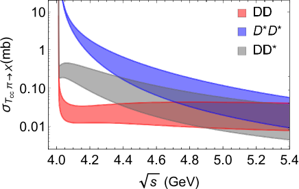
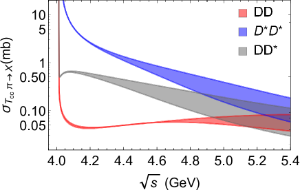
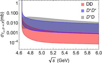
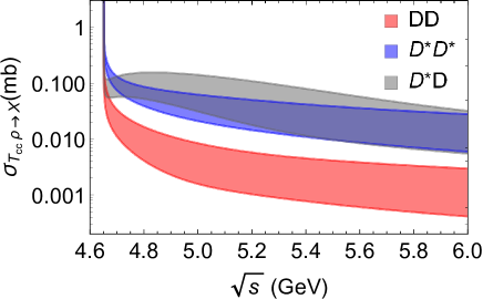
Figure 2: Cross sections for the absorption processes $T_{cc}^{+}\pi\rightarrow D^{(*)}D^{(*)}$ (top panels) and $T_{cc}^{+}\rho\rightarrow D^{(*)}D^{(*)}$ (bottom panels), as functions of the CM energy $\sqrt{s}$. Plots in left and right panels: obtained by using monopole and Gaussian form factors, Eqs. (27) and (28) respectively. Upper and lower limits of the band are obtained taking the upper and lower limits of the cutoff for each corresponding form factor ($1-2$ GeV and $2.5-3.5$ GeV for the monopole and Gaussian form factors, respectively).

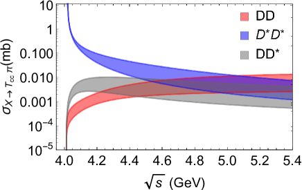
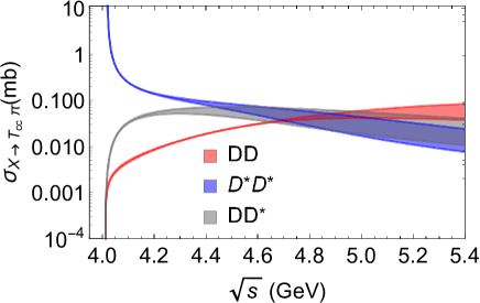
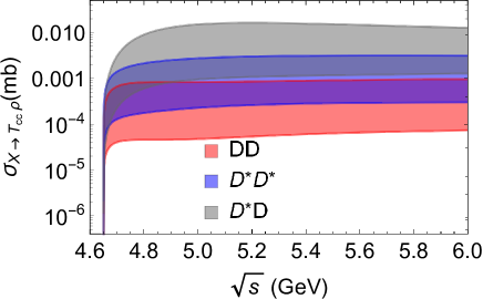
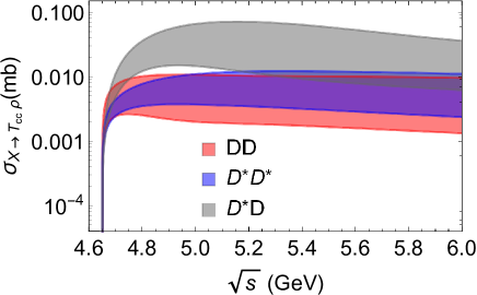
Figure 3: Cross sections as functions of the CM energy $\sqrt{s}$ for the respective inverse (production) processes displayed in Fig. 2, i.e. $D^{(*)}D^{(*)}\rightarrow T_{cc}^{+}\pi$ (top panels) and $D^{(*)}D^{(*)}\rightarrow T_{cc}^{+}\rho$ (bottom panels), obtained via the detailed balance relation. Plots in left and right panels: obtained by using monopole and Gaussian form factors, Eqs. (27) and (27) respectively. Upper and lower limits of the band are obtained taking the upper and lower limits of the cutoff for each corresponding form factor ($1-2$ GeV and $2.5-3.5$ GeV for the monopole and Gaussian form factors, respectively).

Plots of the cross sections as functions of the CM energy $\sqrt{s}$ for the $T_{cc}^{+}$-absorption by pion or $\rho$ mesons are shown in Fig. 2, using monopole and Gaussian form factors defined respectively in Eqs. (27) and (28). Upper and lower limits of the bands are obtained taking the upper and lower limits of the cutoff for each corresponding form factor, i.e. $1-2$ GeV and $2.5-3.5$ GeV for the monopole and Gaussian form factors, respectively.

Since all these absorption cross sections are exothermic (except the one for $T_{cc}\pi\rightarrow D^{*}D^{*}$), they become very large at the threshold. We note that in the region close to the threshold the corresponding curves obtained with and without form factors are almost indistinguishable (we do not display another Figure proving this for the sake of conciseness).

The results suggest that within the range $4.05\leq\sqrt{s}\leq 4.5\mbox{ GeV}$, $\sigma_{T_{cc}\pi\rightarrow X}\,(X=DD,DD^{*},D^{*}D^{*})$ have distinct magnitudes, being of order of $\sim 10^{-3}-1\mbox{ mb}$. Close to the threshold, $\sigma_{T_{cc}\pi\rightarrow DD}$ is suppressed with respect to the other processes, at least by one order of magnitude. However, at higher CM energies ($5\leq\sqrt{s}\leq 5.5\mbox{ GeV}$), all the processes have closer magnitudes.

Looking now at the absorption processes by a $\rho$ meson, which occur at higher thresholds, the $\sigma_{T_{cc}\rho\rightarrow D^{*}D,D^{*}D^{*}}$ are the biggest at moderate energies, while the cross section for $DD$ final states is the smallest. When we compare the different dissociation processes at a given CM energy, for instance $\sqrt{s}=5\mbox{ GeV}$, we observe that $\sigma_{T_{cc}\pi\rightarrow X}$ are greater than the respective $\sigma_{T_{cc}\rho\rightarrow X}$ by about one order of magnitude. These findings allow to quantitatively estimate how big is the contribution coming from the doubly-charmed state absorption by a pion with respect to the other reactions.

Now let us move on to the $T_{cc}^{+}$-production cross sections, which are shown in Fig. 3 as functions of the CM energy, again using both monopole and Gaussian form factors. Except for $\sigma_{D^{*}D^{*}\rightarrow T_{cc}\pi}$, they are endothermic, with magnitudes of the order $\sim 10^{-3}-10^{-1}\mbox{ mb}$ in the case of Gaussian form factor, within the range of CM energies considered. For the monopole, the magnitudes are even smaller. In general, the comparison with the outputs reported in Fig. 2 reveals that both $T_{cc}\pi$ and $T_{cc}\rho$ absorption cross sections are greater than the respective production ones.

IV.2 Form factors from QCDSR

Now we employ the form factors given by Eqs. (23), (25) and (26), obtained within the QCDSR approach. The bands in the figures express the uncertainty in the coupling constant $g_{T_{cc}DD^{*}}$ shown in Eq. (24).

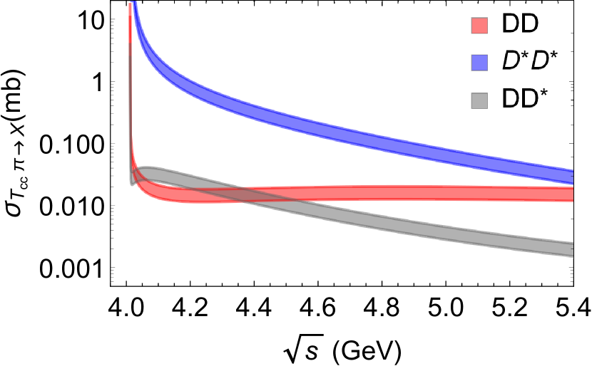
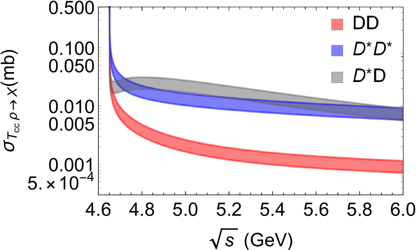
Figure 4: Cross sections for the absorption processes $T_{cc}^{+}\pi\rightarrow D^{(*)}D^{(*)}$ (top panel) and $T_{cc}^{+}\rho\rightarrow D^{(*)}D^{(*)}$ (bottom panel), as functions of the CM energy $\sqrt{s}$, taking the form factors obtained within the QCDSR approach.

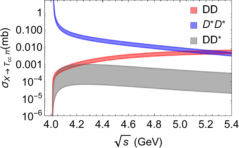
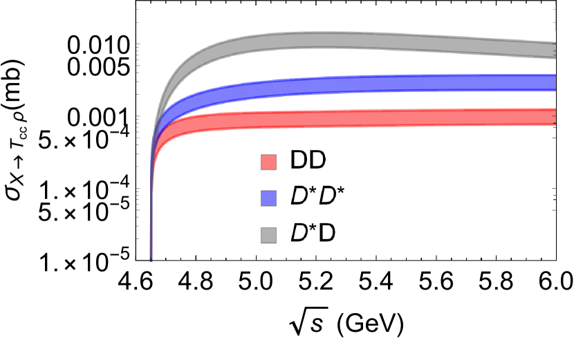
Figure 5: Cross sections as functions of the CM energy $\sqrt{s}$ for the production processes $D^{(*)}D^{(*)}\rightarrow T_{cc}^{+}\pi$ (top panel) and $D^{(*)}D^{(*)}\rightarrow T_{cc}^{+}\rho$ (bottom panel), taking the form factors obtained within the QCDSR approach.).

Figs. 4 and  5 show the plots of the cross sections as functions of the CM energy $\sqrt{s}$ for the $T_{cc}^{+}$-absorption and production by pion or $\rho$ mesons. Some qualitative features found in the preceding subsection (with the empirical form factors) are reproduced. Close to the threshold, cross section $\sigma_{T_{cc}\pi\rightarrow D^{*}D^{*}}$ is greater than the cross sections for other processes. Also, at $\sqrt{s}=5\mbox{ GeV}$, most of cross sections $\sigma_{T_{cc}\pi\rightarrow X}$ are greater than the respective $\sigma_{T_{cc}\rho\rightarrow X}$, although this difference is less pronounced in the present case. Most importantly, both $T_{cc}\pi$ and $T_{cc}\rho$ absorption cross sections are greater than the respective production ones.

There are some differences between the empirical and the QCDSR approach. For example, some reactions in Figs. 4 and  5 have greater magnitudes while others have smaller magnitudes when compared to the corresponding ones in  2 and  3. This is mainly due to the fact that in the QCDSR approach each vertex in a given diagram has a distinct form factor with a specific parametrization according to Eqs. (23)-(26) and Table 1.

Finally, in Fig. 6 we compare our results with those obtained in Ref. Hong:2018mpk . As it can be seen from the figure, our cross sections are significantly smaller than those found in Hong:2018mpk . In comparison to the effective Lagrangian adopted here, in the quasi-free approximation the $T_{cc}^{+}$ is “too easy to destroy”. Part of this difference can be attributed to the couplings and uncertainties associated to the form factors used in each work.

In Fig. 6 we can observe that the results obtained with the empirical and the QCDSR form factors are not so different. This is not unexpected, since the form factors are calibrated with coupling constants, which, in some vertices, were the same and derived from QCDSR. So, in fact, most of the difference in the cross sections comes from how the form factor decreases with increasing $Q^{2}$.

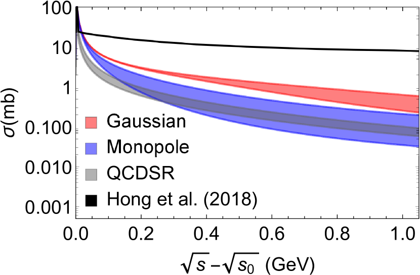
Figure 6: Sum of the cross sections for the processes obtained in this work ($T_{cc}\pi\rightarrow DD+DD^{*}+D^{*}D^{*}$) and in Ref. Hong:2018mpk ($T_{cc}\pi\rightarrow D\pi+D^{*}\pi$ ), as a function of the CM energy $\sqrt{s}$ above the threshold energy $\sqrt{s_{0}}$ of each process. The legend denotes the respective functional form of form factors used to calculate the cross sections.

In the end, the final results contain large uncertainties, but they still carry valuable information. Despite all uncertainties, it remains true that $T_{cc}$ absorption is stronger than its creation. This result is not surprising and a similar dominance of absorption over production was found in the case of $J/\psi$, $\Upsilon$, and other multiquark states such as the $X(3872)$ and $Z_{b}$.

Once the vacuum cross sections are known, the next step is to compute the thermal cross sections, which are convolutions of the vacuum cross sections with thermal momentum distributions of the colliding particles. In this approach, the temperature of the hadron gas (which is in the range 100 - 200 MeV) determines the collision energy. When we perform this thermal average, the kinematical configurations close to the thresholds are highly suppressed. Hence the strong threshold enhancement (or suppression) observed in all the figures above have little significance for applications to heavy ion collisions.

V Concluding remarks

The purpose of this work has been to study, from an effective framework, the interactions of the doubly charmed tetraquark state $T_{cc}^{+}$ with light mesons in the hadron gas phase. Their absorption and production processes have been computed, deserving special attention to the role of the form factor of the $T_{cc}-D-D^{*}$ coupling, obtained from QCD sum rules.

The results suggest sizeable cross sections for the considered processes. Moreover, the $T_{cc}^{+}$ absorption in a hadron gas appears to be more important than its production. On the other hand, when compared with the other existing estimate, our approach suggests much smaller $T_{cc}^{+}$ absorption cross sections than those of Ref. Hong:2018mpk , based on the quasi-free approximation.

The obtained $T_{cc}^{+}$ production and absorption cross sections will be crucial for a comprehensive analysis of the evolution of the $T_{cc}^{+}$ abundance in heavy ion collisions. This is another observable useful to shed light on the $T_{cc}^{+}$ internal structure. This study is in progress and we expect to publish it soon.

References

• (1) R. Aaij et al. [LHCb], [arXiv:2109.01038 [hep-ex]].
• (2) R. Aaij et al. [LHCb], [arXiv:2109.01056 [hep-ex]].
• (3) B. A. Gelman and S. Nussinov, Phys. Lett. B 551, 296 (2003).
• (4) D. Janc and M. Rosina, Few Body Syst. 35, 175 (2004).
• (5) J. Vijande, F. Fernandez, A. Valcarce and B. Silvestre-Brac, Eur. Phys. J. A 19, 383 (2004).
• (6) F. S. Navarra, M. Nielsen and S. H. Lee, Phys. Lett. B 649, 166 (2007).
• (7) J. Vijande, E. Weissman, A. Valcarce and N. Barnea, Phys. Rev. D 76, 094027 (2007).
• (8) D. Ebert, R. N. Faustov, V. O. Galkin and W. Lucha, Phys. Rev. D 76, 114015 (2007).
• (9) S. H. Lee and S. Yasui, Eur. Phys. J. C 64, 283 (2009).
• (10) Y. Yang, C. Deng, J. Ping and T. Goldman, Phys. Rev. D 80, 114023 (2009).
• (11) J. Hong, S. Cho, T. Song and S. H. Lee, Phys. Rev. C 98, 014913 (2018).
• (12) R. J. Hudspith, B. Colquhoun, A. Francis, R. Lewis and K. Maltman, Phys. Rev. D 102, 114506 (2020).
• (13) J. B. Cheng, S. Y. Li, Y. R. Liu, Z. G. Si and T. Yao, Chin. Phys. C 45, 043102 (2021).
• (14) Q. Qin, Y. F. Shen and F. S. Yu, Chin. Phys. C 45, 103106 (2021).
• (15) S. S. Agaev, K. Azizi and H. Sundu, [arXiv:2108.00188 [hep-ph]].
• (16) X. K. Dong, F. K. Guo and B. S. Zou, [arXiv:2108.02673 [hep-ph]].
• (17) Y. Huang, H. Q. Zhu, L. S. Geng and R. Wang, Phys. Rev. D 104, 116008 (2021).
• (18) N. Li, Z. F. Sun, X. Liu and S. L. Zhu, Chin. Phys. Lett. 38, 092001 (2021).
• (19) H. Ren, F. Wu and R. Zhu, [arXiv:2109.02531 [hep-ph]].
• (20) Q. Xin and Z. G. Wang, [arXiv:2108.12597 [hep-ph]].
• (21) G. Yang, J. Ping and J. Segovia, [arXiv:2109.04311 [hep-ph]].
• (22) L. Meng, G. J. Wang, B. Wang and S. L. Zhu, Phys. Rev. D 104, 051502 (2021).
• (23) X. Z. Ling, M. Z. Liu, L. S. Geng, E. Wang and J. J. Xie, [arXiv:2108.00947 [hep-ph]].
• (24) S. Fleming, R. Hodges and T. Mehen, [arXiv:2109.02188 [hep-ph]].
• (25) Y. Jin, S. Y. Li, Y. R. Liu, Q. Qin, Z. G. Si and F. S. Yu, [arXiv:2109.05678 [hep-ph]].
• (26) K. Azizi and U. Özdem, [arXiv:2109.02390 [hep-ph]].
• (27) Y. Hu, J. Liao, E. Wang, Q. Wang, H. Xing and H. Zhang, [arXiv:2109.07733 [hep-ph]].
• (28) L. W. Chen, C. M. Ko, W. Liu and M. Nielsen, Phys. Rev. C 76, 014906 (2007); F. S. Navarra, M. Nielsen, M. E. Bracco, M. Chiapparini and C. L. Schat, Phys. Lett. B 489, 319 (2000); F. S. Navarra, M. Nielsen and M. E. Bracco, Phys. Rev. D 65, 037502 (2002).
• (29) S. Cho and S. H. Lee, Phys. Rev. C 88, 054901 (2013); M. E. Bracco, M. Chiapparini, F. S. Navarra and M. Nielsen, Phys. Lett. B 659, 559 (2008).
• (30) A. Martinez Torres, K. P. Khemchandani, F. S. Navarra, M. Nielsen and L. M. Abreu, Phys. Rev. D 90, 114023 (2014); A. Martinez Torres, K. P. Khemchandani, F. S. Navarra, M. Nielsen and L. M. Abreu, Acta Phys. Pol. B Proc. Supp. 8, 247 (2015).
• (31) L. M. Abreu, K. P. Khemchandani, A. Martinez Torres, F. S. Navarra and M. Nielsen, Phys. Lett. B 761, 303 (2016).
• (32) L. M. Abreu, K. P. Khemchandani, A. Martinez Torres, F. S. Navarra, M. Nielsen and A. L. Vasconcellos, Phys. Rev. D 95, 096002 (2017).
• (33) A. Martínez Torres, K. P. Khemchandani, L. M. Abreu, F. S. Navarra and M. Nielsen, Phys. Rev. D 97, 056001 (2018).
• (34) L. M. Abreu, K. P. Khemchandani, A. Martínez Torres, F. S. Navarra and M. Nielsen, Phys. Rev. C 97, 044902 (2018).
• (35) L. M. Abreu, F. S. Navarra and M. Nielsen, Phys. Rev. C 101, 014906 (2020).
• (36) C. Le Roux, F. S. Navarra and L. M. Abreu, Phys. Lett. B 817, 136284 (2021).
• (37) A. Andronic, P. Braun-Munzinger, M. K. Köhler, K. Redlich and J. Stachel, Phys. Lett. B 797, 134836 (2019).
• (38) A. Andronic, P. Braun-Munzinger, M. K. Köhler, A. Mazeliauskas, K. Redlich, J. Stachel and V. Vislavicius, JHEP 07, 035 (2021).
• (39) S. G. Matinyan and B. Müller, Phys. Rev. C 58, 2994 (1998); Y. Oh, T. Song and S. H. Lee, Phys. Rev. C 63, 034901 (2001); F. Carvalho, F. O. Duraes, F. S. Navarra and M. Nielsen, Phys. Rev. C 72, 024902 (2005); B. Osorio Rodrigues, M. E. Bracco, M. Nielsen and F. S. Navarra, Nucl. Phys. A 852, 127 (2011).
• (40) M.A. Shifman, A.I. and Vainshtein and V.I. Zakharov, Nucl. Phys. B 147, 385 (1979).
• (41) L.J. Reinders, H. Rubinstein and S. Yazaki, Phys. Rept. 127, 1 (1985).
• (42) M.E. Bracco, M. Chiapparini, F.S. Navarra and M. Nielsen, Prog. Part. Nucl. Phys.  67, 1019 (2012).
• (43) V. M. Belyaev, V. M. Braun, A. Khodjamirian and R. Ruckl, Phys. Rev. D 51, 6177 (1995).
• (44) A. Khodjamirian, B. Melić, Y. M. Wang and Y. B. Wei, JHEP 03, 016 (2021).
• (45) J. M. Dias, F. S. Navarra, M. Nielsen and C. M. Zanetti, Phys. Rev. D 88, 016004 (2013).
• (46) B.L. Ioffe and A.V. Smilga, Nucl. Phys. B 232, 109 (1984).
• (47) P. A. Zyla et al. [Particle Data Group], PTEP 2020, 083C01 (2020).