Making the computation of approximations of invariant measures and its attractors for IFS and GIFS, through the deterministic algorithm, tractable

Abstract

We present algorithms to compute approximations of invariant measures and its attractors for IFS and GIFS, using the deterministic algorithm in a tractable way, with code optimization strategies and use of data structures and search algorithms. The results show that these algorithms allow the use of these (G)IFS in a reasonable running time.

2010 MSC Classification]Primary: 28A80, 28A33, 37M25; Secondary: 37C70, 54E35, 65S05, 68P05, 68P10

1 Introduction

The Hutchinson–Barnsley theory for IFS seek to establish the existence of an unique attractor set, invariant by the fractal operator, and an unique measure of probability with support on the attractor, invariant by the Markov operator. Those objects are of paramount importance in the extensive applications in several fields of pure and applied sciences.

There are mainly three types of algorithms to approximate the attractor and the invariant measure. The deterministic one, where and initial set or measure is iterated by the respective operators approximating the attractor or the invariant measure w.r.t. the appropriated topology, see Bar ; BDEG for classical IFS and JMS16 for GIFS. The discrete one, is similar to the deterministic but an initial step is to introduce a discrete version of the space, an $\varepsilon$-net, and a discrete version of the operator, which is then iterated in the same fashion as the deterministic one producing a discrete set close to the attractor and a discrete measure which is close to the invariant one, GN ; GMN ; COS21 . For the last, we have several variations of the original chaos game algorithm introduce by M. Barnsley, Bar , where an initial point is iterated choosing, according to some probability, the function to be used. As the process goes on its orbit approximates the attractor set.

As can be seen in MM3 ; GN ; GMN and COS20 ; COS21 the discrete algorithms exhibit a good performance, but require a lot of technical detail to its implementation. On the other hand deterministic algorithms are easy to describe and implement, in its naive version, but they are impractical computationally. Our aim is to improve this feature.

As described in the sequel, we are interested in deterministic algorithms for IFS and GIFS that require a search for a given value over very large sets of points. A case where it occurs is the approximation of the invariant measure for an IFS or GIFS by iterating the Markov operator from a single point of mass. This task is particularly hard for Idempotent IFS and GIF due its nature.

There are many search algorithms that are tailored to perform geometric scans of a region to locate an specific point, and they all use some form of hierarchical partitioning of the region. In our case, algorithms that deal with discrete representations of the points (for instance, line or column ordering of pixels) are not suited. Instead, we have opted to use a rectangular, regular partition of the region into four quadrants, which leads to the use of quadtrees, a well-known data structure (see Finkel1974 , HS1984 , HS1988 and SHP2011 , to cite just a few). This is coupled with a fast indexing function to locate quadrants of ever diminishing area, whose limits bracket the point being sought for.

The paper is organized as follows. Section 2 recalls the Hutchinson–Barnsley theory. In Section 3 we state the deterministic algorithm for IFS, followed by the introduction of our quadtree-based search algorithm on Section 4. The natural extension of these algorithms to GIFS is given on Section 6. Finally, we conclude with our remarks on Section 7.

2 The Hutchinson–Barnsley theory

For the convenience of the reader, we will now recall a few basic facts on Iterated Function Systems (IFS for short) and Generalized Iterated Function Systems (GIFS for short).
Let $(X,d)$ be a complete, Haussdorf metric space. By an IFS with probabilities we mean a triple $\mathcal{S}=(X,(\phi_{j})_{j=1}^{L},(p_{j})_{j=1}^{L})$ so that $\phi_{j}:X\to X$ and $(X,(\phi_{j})_{j=1}^{L})$ is an IFS and $p_{1},...,p_{L}\geq 0$ with $\sum_{j=1}^{L}p_{j}=1$. Since IFS are widely known in the literature we will avoid to repeat those definitions for GIFS because they are almost equal, except by the fact that $\phi_{j}:X\times X\to X$. Each IFS $\mathcal{S}=(X,(\phi_{j})_{j=1}^{L})$ generates the Hutchinson–Barnsley operator $F_{\mathcal{S}}:\mathcal{K}(X)\to\mathcal{K}(X)$, where $\mathcal{K}(X)$ is the set of nonempty compact sets of $X$, defined by $\displaystyle\forall_{K\in\mathcal{K}(X)}\;F_{\mathcal{S}}(K):=\bigcup_{j=1}^{L}\phi_{j}(K).$ A set $A_{\mathcal{S}}\in\mathcal{K}(X)$ is called the attractor of the IFS $\mathcal{S}$, if $A_{\mathcal{S}}=F_{\mathcal{S}}(A_{\mathcal{S}})$ and for every $K\in\mathcal{K}(X)$, the sequence of iterations $F_{\mathcal{S}}^{(n)}(K)\to A_{\mathcal{S}}$ w.r.t. the Hausdorff metric.
Each IFSp generates also the map $M_{\mathcal{S}}:\mathcal{P}(X)\to\mathcal{P}(X)$, called the Markov operator, which adjust to every $\mu\in\mathcal{P}(X)$, the measure $M_{\mathcal{S}}(\mu)$ defined by $\displaystyle M_{\mathcal{S}}(\mu)(B)=\sum_{j=1}^{L}p_{j}\mu\left(\phi_{j}^{-1}(B)\right)$, for any Borel set $B\subset X$.
By an invariant measure of an IFSp $\mathcal{S}$ we mean a (necessarily unique) measure $\mu_{\mathcal{S}}\in\mathcal{P}(X)$ which satisfies $\mu_{\mathcal{S}}=M_{\mathcal{S}}(\mu_{\mathcal{S}})$ and such that for every $\mu\in\mathcal{P}(X)$, the sequence of iterates $M^{k}_{\mathcal{S}}(\mu)$ converges to $\mu_{\mathcal{S}}$ with respect to the Monge–Kantorovich distance. The Markov operator $M_{\mathcal{S}}$, is also characterized by

$$\int_{X}f\;dM_{\mathcal{S}}(\mu)=\sum_{j=1}^{L}p_{j}\int_{X}f\circ\phi_{j}\;d\mu,$$ (1)

for every IFSp $\mathcal{S}$ and every continuous map $f:X\to\mathbb{R}$. The following result is known (see, for example (Hut, , Section 4.4)).

Theorem 2.1.

Each IFSp on a complete metric space consisting of Banach contractions admits an invariant measure.

The Lemma 5.1, from COS21 , is the basis for the deterministic algorithm, Algorithm 1. Starting with an initial measure of probability $\mu=\delta_{x_{0}}\in\mathcal{P}(X)$, each iteration produces a new measure $M_{\mathcal{S}}(\mu),M_{\mathcal{S}}^{2}(\mu),...$, converging to the invariant measure, whose weight in each point of the support, described below, requires to compute the weights of all points which has the same image. Additionally, the set of supporting points describe the deterministic algorithm to approximate de attractor. If for some $N\geq 1$ we have $M_{\mathcal{S}}^{N}(\mu)=\sum_{i=1}^{m}v_{i}\delta_{y_{i}}\in\mathcal{P}(X)$, that is, each $v_{i}\geq 0$ and $\sum_{i=1}^{m}v_{i}=1$, then

$$\operatorname{supp}(M_{\mathcal{S}}^{N+1}(\mu))=\{\phi_{j}(y_{i}):j=1,...,L,\;i\in\{1,...,m\}\}$$ (2)

and enumerating this set by $\{z_{1},...,z_{m^{\prime}}\}$, we have:

$$M_{\mathcal{S}}^{N+1}(\mu)=\sum_{r=1}^{m^{\prime}}v^{\prime}_{r}\delta_{z_{r}},$$ (3)

where $\displaystyle v^{\prime}_{r}=\sum_{\phi_{j}(y_{i})=z_{r}}p_{j}v_{i}$.
In other words, the discrete algorithm starts with a product set $D_{0}=\{(x_{0},1)\}$ which is the initial value and, at each iteration, the set $D_{N}=\{(y_{1},v_{1}),...,(y_{m},v_{m})\}$ is updated by the application of the Markov operator producing the new set

$$D_{N+1}=\{(z_{1},v^{\prime}_{1}),...,(z_{m^{\prime}},v^{\prime}_{m^{\prime}})\},$$

obtained by the updating rule (3). The first coordinates of $D_{N}$, given by $\operatorname{supp}(M_{\mathcal{S}}^{N+1}(\mu))$ approximate the attractor set $A_{\mathcal{S}}$, and the second coordinates $\{v^{\prime}_{1},...,v^{\prime}_{m^{\prime}}\}$, gives the value at each point of the discrete probability $M_{\mathcal{S}}^{N}(\mu)$ approximating the invariant probability $\mu_{\mathcal{S}}$.
For a GIFS the updating rule is almost the same, if $M_{\mathcal{S}}^{N}(\mu)=\sum_{i=1}^{m}v_{i}\delta_{y_{i}}\in\mathcal{P}(X)$, that is, each $v_{i}\geq 0$ and $\sum_{i=1}^{m}v_{i}=1$, then

$$\operatorname{supp}(M_{\mathcal{S}}^{N+1}(\mu))=\{\phi_{j}(y_{i_{0}},y_{i_{1}}):j=1,...,L,\;i_{0},i_{1}\in\{1,...,m\}\}$$ (4)

and enumerating this set by $\{z_{1},...,z_{m^{\prime}}\}$, we have:

$$M_{\mathcal{S}}^{N+1}(\mu)=\sum_{r=1}^{m^{\prime}}v^{\prime}_{r}\delta_{z_{r}},$$ (5)

where $\displaystyle v^{\prime}_{r}=\sum_{\phi_{j}(y_{i_{0}},y_{i_{1}})=z_{r}}p_{j}v_{i_{0}}v_{i_{1}}$.
In MZ and more recently in dacunha2021fuzzyset there was considered the following version in the context of idempotent measures. Let $\mathbb{R}_{{\rm max}}:=\mathbb{R}\cup\{-\infty\}$ be the extended set of real numbers. Consider the operations $x\oplus y=\max\{x,y\}$ and $x\odot y=x+y$. Then we define the max-plus semiring $S$ as the algebraic structure $S=(\mathbb{R}_{{\rm max}},\oplus,\odot)$. A functional $\mu:C(X)\to\mathbb{R}$ satisfying

1. $\mu(\lambda)=\lambda$ for all $\lambda\in\mathbb{R}$ (normalization);

2. $\mu(\lambda\odot\psi)=\lambda\odot\mu(\psi)$, for all $\lambda\in\mathbb{R}$ and $\psi\in C(X)$;

3. $\mu(\varphi\oplus\psi)=\mu(\varphi)\oplus\mu(\psi)$, for all $\varphi,\psi\in C(X)$,

is called an idempotent probability measure (or Maslov measure), Z ; Zai . A key idea is the density of an idempotent probability measure introduced in Kol88 . If $\lambda:X\to[-\infty,0]$ is upper semicontinuous and $\lambda(x)=0$ for some $x\in X$, then the map $\displaystyle\mu_{\lambda}=\bigoplus_{x\in X}\lambda(x)\odot\delta_{x}$ is an idempotent measure, that is, $\mu_{\lambda}\in I(X)$. The density $\lambda_{\mu}$ of $\mu\in I(X)$ is uniquely determined.
Let $\mathcal{S}=(X,(\phi_{j})_{j=1}^{m})$ be an IFS and $(q_{j})_{j=1}^{L}$ is a family of real numbers so that $q_{j}\leq 0$ for $j=1,...,L$ and, $\displaystyle\bigoplus_{j=1,...,L}q_{j}=0$. Then we call the triple $\mathcal{S}_{\operatorname{mp}}=(X,(\phi)_{j=1}^{L},(q_{j})_{j=1}^{L})$ as a max-plus normalized IFS (which is the idempotent analogous of the IFSp). Each max-plus normalized IFS $\mathcal{S}_{\operatorname{mp}}=(X,(\phi_{j})_{j=1}^{L},(q_{j})_{j=1}^{L})$ generates the map $M_{\mathcal{S}}:I(X)\to I(X)$, called as the idempotent Markov operator, which adjust to every $\mu\in I(X)$, the idempotent measure $M_{\mathcal{S}}(\mu)$ defined by:

$$M_{\mathcal{S}}(\mu):=\bigoplus_{j=1}^{L}q_{j}\odot(I(\phi_{j})(\mu))$$

that is, for every $\psi\in C(X)$, $M_{\mathcal{S}}(\mu)({\psi})=\bigoplus_{j=1}^{L}q_{j}\odot\mu({\psi}\circ\phi_{j})$, because $I(\phi_{j})(\mu)(\psi):=\mu({\psi}\circ\phi_{j})$.
By an invariant idempotent measure of a max-plus normalized IFS $\mathcal{S}_{\operatorname{mp}}$ we mean the unique measure $\mu_{\mathcal{S}}\in I(X)$ which satisfies

$$\mu_{\mathcal{S}}=M_{\mathcal{S}}(\mu_{\mathcal{S}})$$

and such that for every $\mu\in I(X)$, the sequence of iterates $M^{(n)}_{\mathcal{S}}(\mu)$ converges to $\mu_{\mathcal{S}}$ with respect to the $\tau_{p}$ topology on $I(X)$.
We say that a max-plus normalized IFS $\mathcal{S}_{\operatorname{mp}}$ is Banach contractive, if the underlying IFS ${\mathcal{S}}$ is contractive. The main result of MZ , that is (MZ, , Theorem 1), states that:

Theorem 2.2.

Each Banach contractive max-plus normalized IFS $\mathcal{S}_{\operatorname{mp}}$ on a complete metric space generates the unique invariant idempotent measure $\mu_{\mathcal{S}}$.

We notice that Theorem 2.2 was extended in several ways in our recent works dacunha2021fuzzyset and dacunha2021existence .

Now we give a description of the Idempotent Markov operator acting on a finite measure, which is an application of Lemma 5.5 from dacunha2021fuzzyset . For $\mu=\bigoplus_{x\in X}\lambda(x)\odot\delta_{x}\in I(X)$, we have that

$$M_{\mathcal{S}}(\mu)=\bigoplus_{y\in X}\lambda_{\mathcal{S}}(y)\odot\delta_{y}$$

where

$$\lambda_{\mathcal{S}}(y)=\left\{\begin{array}[]{cc}\max\{q_{j}+\lambda(x):j=1,...,L,\;x\in\phi^{-1}_{j}(y)\},&\mbox{if}\;y\in\bigcup_{j=1}^{L}\phi_{j}(X)\\ -\infty,&\mbox{otherwise}\end{array}\right..$$

Analogously to the classic IFS, if we start with a singleton $\mu=\delta_{x_{0}}\in I(X)$, the deterministic method consists in to iterate $M_{\mathcal{S}}(\mu),M_{\mathcal{S}}^{2}(\mu),...$ which are also discrete measures with support in a discrete set, converging to the invariant one:
In the above frame, if for some $N\geq 1$ we have $M_{\mathcal{S}}^{N}(\mu)=\bigoplus_{i=1}^{m}v_{i}\odot\delta_{y_{i}}\in I(X)$, that is, each $v_{i}\leq 0$ and $\bigoplus_{i=1}^{m}v_{i}=0$, then

$$\operatorname{supp}(M_{\mathcal{S}}^{N+1}(\mu))=\{\phi_{j}(y_{i}):j=1,...,L,\;i=\{1,...,m\}\}$$ (6)

and enumerating this set by $\{z_{1},...,z_{m^{\prime}}\}$, we have:

$$M_{\mathcal{S}}^{N+1}(\mu)=\bigoplus_{r=1}^{m^{\prime}}v^{\prime}_{r}\odot\delta_{z_{r}},$$ (7)

where $\displaystyle v^{\prime}_{r}=\max_{\phi_{j}(y_{i})=z_{r}}q_{j}+v_{i}$.
In other words, the discrete algorithm starts with a direct product set $D_{0}=\{(x_{0},1)\}$ which is the initial value and, at each iteration, the set $D_{N}=\{(y_{1},v_{1}),...,(y_{m},v_{m})\}$ is updated by the application of the idempotent Markov operator producing the new set

$$D_{N+1}=\{(z_{1},v^{\prime}_{1}),...,(z_{m^{\prime}},v^{\prime}_{m^{\prime}})\},$$

obtained by the updating rule (7). The first coordinates of $D_{N}$, given by $\operatorname{supp}(M_{\mathcal{S}}^{N+1}(\mu))$ approximate the attractor set $A_{\mathcal{S}}$, and the second coordinates $\{v^{\prime}_{1},...,v^{\prime}_{m^{\prime}}\}$, gives the value at each point of the discrete probability $M_{\mathcal{S}}^{N}(\mu)$ approximating the invariant idempotent probability $\mu_{\mathcal{S}}$.
For an Idempotent GIFS, if $M_{\mathcal{S}}^{N}(\mu)=\bigoplus_{i=1}^{m}v_{i}\odot\delta_{y_{i}}\in I(X)$, that is, each $v_{i}\leq 0$ and $\bigoplus_{i=1}^{m}v_{i}=0$, then

$$\operatorname{supp}(M_{\mathcal{S}}^{N+1}(\mu))=\{\phi_{j}(y_{i_{0}},y_{i_{1}}):j=1,...,L,\;i_{0},i_{1}\in\{1,...,m\}\}$$ (8)

and enumerating this set by $\{z_{1},...,z_{m^{\prime}}\}$, we have:

$$M_{\mathcal{S}}^{N+1}(\mu)=\bigoplus_{r=1}^{m^{\prime}}v^{\prime}_{r}\odot\delta_{z_{r}},$$ (9)

where $\displaystyle v^{\prime}_{r}=\max_{\phi_{j}(y_{i_{0}},y_{i_{1}})=z_{r}}q_{j}+v_{i_{0}}+v_{i_{1}}$.
For additional facts on Hutchinson–Barnsley theory for IFS see Bar . For additional facts on idempotent IFS see Z ; MZ ; Zai . We will not state the analogous facts for GIFS to avoid repetitions; these can be found in GMM ; Mi ; MM ; MM1 .

3 Deterministic Algorithm for IFS

The standard deterministic algorithm to compute an approximation of both the attractor and the associated invariant measure for an IFS, or an Idempotent IFS, is given in the Algorithm 1. To avoid extra technicalities we will work with 2D contained in a rectangle $[a\mathchar 24635\relax\;b]\times[c\mathchar 24635\relax\;d]$.

A number $N$ of iterations is set and a set of $L$ functions $\phi_{i}:\mathbb{R}^{2}\rightarrow\mathbb{R}^{2}$, $1\leq i\leq L$ which describe the attractor is given. The iterations are started over a single point with coordinates $(x,y)$ such that $a\leq x\leq b$ and $c\leq y\leq b$ and some property $p$ associated with that point (say, $p=0$). The output is an array $D$ of triplets $(x,y,p)$. The number of triplets stored in $D$ is referred to by $D.n$.

Algorithm 1 Deterministic Algorithm for IFS

1:function Deterministic_IFS(input: $N,L,x,y,p$; output: $D$)

2:$N$, number of iterations

3:$L$, number of $\phi_{i}$ functions

4:$(x,y)$, coordinates of initial point

5:$p$, some property of the initial point

6:$D$, array of $(x,y,p)$ triplets Local: $T$, array of $(x,y,p)$ triplets

7:     $D.n\leftarrow 1$

8:     $D[D.n]\leftarrow(x,y,p)$

9:     for $i\leftarrow 1$ to $N$ do

10:         $T.n\leftarrow 0$ // initialize the number of triplets stored in $T$

11:         for $j\leftarrow 1$ to $L$ do

12:              for $k\leftarrow 1$ to $D.n$ do

13:                  $(u,v)\leftarrow\phi_{j}(D[k].x,D[k].y)$

14:                  initialize $r$ with some appropriate value

15:                  search for $(u,v)$ in $T$

16:                  if $(u,v)$ is not in $T$ then

17:                       $T.n\leftarrow T.n+1$

18:                       $T[T.n]\leftarrow(u,v,r)$

19:                  else

20:                       // $m$ is the index in $T$ such that $T[m].(x,y)=(u,v)$

21:                       update the value of $p$ in the triplet $T[m]$ (using $r$)

22:                  end if

23:              end for

24:         end for

25:         $D\leftarrow T$

26:     end for

27:end function

The algorithm is written as it would be suitable to compute the invariant measure whose support is the attractor. To this end, a search (line 15 of Algorithm 1) for a point $(u,v)$ that has been produced from a point $D[k]$ produced in the previous iteration, with an associated property $r$, is made over the points being produced in the current iteration (which are stored on a local array $T$ of triplets $(x,y,p)$ similar to $D$). If $(u,v)$ is found on $T$, then its associated property $p$ is modified, dependent on how the measure is defined: that could be expressed as the maximum between, or a sum involving $p$ and $r$.

We note that $p$ is updated (Algorithm 1, line 21) according to Equation (3) (for classic IFS) and to Equation (7) (for idempotent IFS). For the latter, the variable $r$ is initialized with $p_{j}+D[k].p$ and the update is $T[m].p\leftarrow\max(T[m].p,r)$.

Of course, if one does not wish to compute such a measure, then the algorithm becomes much simpler: there is no need to perform any searches and it is just a matter of applying the $\phi_{i}$ functions over the set of points produced at the previous iteration.

The main issue arising with Algorithm 1 (or, indeed, with its simpler version) is that the number of points produced at each iteration grow considerably, to a point where it becomes impracticable to execute it in a reasonable time, or simply the amount of memory required to store the points in the arrays $D$ and $T$ is not available. Another issue, one that becomes much more noticeable as the iterations proceed, is the number of operations required to search for $(u,v)$ in $T$.

4 Optimizing Algorithm 1 using a better search algorithm

As seen above, the use of a linear search leads to an overall cost in terms of the number of searches that is exponential in nature. It is not possible to reduce this exponential growth, because it is the very essence of Algorithm 1; however, we can make it more tractable if a better search algorithm is employed. This may allow, for instance, to perform one more iteration in Algorithm 1, and that may be just enough to obtain a good image of the attractor, or a more refined value for the measure being computed.

Since an IFS produces an image that is fractal in nature and it has a contractivity property, the attractor is a compact set, meaning that the points generated along the iterations will all fall within a suitable rectangular region $X=[a\mathchar 24635\relax\;b]\times[c\mathchar 24635\relax\;d]$ in $\mathbb{R}^{2}$ such that any point with coordinates $(x,y)$ along the Cartesian axes satisfy $a\leq x\leq b$ and $c\leq y\leq b$, a hierarchical subdivision of the rectangular region is well indicated to help one to obtain a faster search algorithm. This leads to the use of a quadtree to organize the points and ease searching for one, as the search can be done only on the regions where a particular point resides, discarding all the others.

Given the intervals $[a\mathchar 24635\relax\;b]$ and $[c\mathchar 24635\relax\;d]$, we proceed by computing their midpoints $m_{x}$ and $m_{y}$. With these six values the limits of four quadrants can be defined, as in Figure 1. Each quadrant is then assigned a two-bit Gray code, in which the code between two neighbouring quadrants (i.e. those that share a common edge) differs by just one bit. Thus, the quadrants are enumerated from $0$ to $3$.

Figure 1: Dividing a region into four quadrants; each quadrant is uniquely identified by a two-bit Gray code.

We now define the function $Q(x,y)$ which gives the quadrant number as follows:

$$Q(x,y) = 2i(y,c,d)+i(x,a,b)$$ (10)

$$i(v,\alpha,\beta) = \left\{\begin{array}[]{cc}0,&\frac{v-\alpha}{\beta-\alpha}<\frac{1}{2}\\ 1,&\emph{otherwise}\end{array}\right.,\alpha\leq v\leq\beta$$ (13)

where $0\leq Q(x,y)\leq 3$. Therefore, any point within the region may be attributed to a unique quadrant (we may also refer to the value returned by $Q(x,y)$ in terms of its related two-bit Gray code).

The quadtree data structure is made up of nodes associated to quadrants. Its root node, of course, refers to the region $X$ as defined before. Each node stores the values $a,b,c,d$ along the $x$ and $y$ axes that define the quadrant region. If there are any points within its region, the node will also store an array of integer values $I$ with at most $n_{\max}$ entries. This array contains the indices of the points stored in $T$ (on Algorithm 1) which belong to the quadrant.

The node may also hold four node sons, in case it has been divided when trying to insert a point on the quadtree. This will happen whenever a node $K$ was supposed to hold a point $(x,y)$ for which $Q(x,y)=k$, but the array $I_{K}$ has no more free entries. In this case, the node is subdivided into four sons, by the midpoints of $[a\mathchar 24635\relax\;b]$ and $[c\mathchar 24635\relax\;d]$, as in Figure 1. The points associated to node(quadrant) $K$ are redistributed among its sons and, finally, the point that was being inserted (and caused the subdivision) is assigned to one of its sons, recursively. Only leaf nodes (i.e. nodes without sons) have the array $I$ and any search for a point $(x,y)$ occurs only on a leaf node.

These ideas are presented in Algorithm 2. We also present Algorithm 3, which is a modification of Algorithm 1 to use the quadtree data structure.

Algorithm 2 Quadtree search and insert

1:function Quadtree_Search_and_Insert(input: $Q,u,v,r$; output: $D$)

2:$Q$, a quadtree node

3:$(u,v)$, coordinates of point to search

4:$r$, some property of the point to search

5:$D$, array of $(x,y,p)$ triplets

6:     if node $Q$ has sons then

7:         $i\leftarrow Q(u,v)$

8:         Quadtree_Search_and_Insert($Q.sons[i],u,v,r,D$)

9:     else

10:         $f\leftarrow 0$

11:         for $j\leftarrow 1$ to $Q.I.n$ do

12:              // linear search for $(u,v)$ on $Q.I$

13:              if $u=D[Q.I[j]].x$ AND $v=D[Q.I[j]].y$ then

14:                  update the value of $p$ in the triplet $D[Q.I[j]]$ (using $r$)

15:                  $f\leftarrow 1$

16:                  break

17:              end if

18:         end for

19:         if $f=0$ then

20:              // if $(u,v)$ was not found on $Q.I$

21:              if $Q.I.n<n_{\max}$ then

22:                  // if there are free entries available on $Q.I$,

23:                  // add $(u,v)$ to $D$ and its index to $Q.I$

24:                  $D.n\leftarrow D.n+1$

25:                  $D[D.n]\leftarrow(u,v,r)$

26:                  $Q.I.n\leftarrow Q.I.n+1$

27:                  $Q.I[Q.I.n]\leftarrow D.n$

28:              else

29:                  divide node $q$ into four sons

30:                  for $j\leftarrow 1$ to $Q.I.n$ do

31:                       // distribute the indices of $Q$ among its sons

32:                       $i\leftarrow Q(D[q.I[j]].x,D[q.I[j]].y)$

33:                       $Q.sons[i].I.n\leftarrow Q.sons[i].I.n+1$

34:                       $Q.sons[i].I[Q.sons[i].I.n]\leftarrow Q.I[j]$

35:                  end for

36:                  // insert $(u,v,r)$ into the appropriate son of $Q$

37:                  $i\leftarrow Q(u,v)$

38:                  Quadtree_Search_and_Insert($Q.sons[i],u,v,r,D$)

39:              end if

40:         end if

41:     end if

42:end function

Algorithm 3 Deterministic Algorithm for IFS with quadtree-based search

1:function Deterministic_IFS_quadtree(input: $N,L,x,y,p$; output: $D$)

2:$N$, number of iterations

3:$L$, number of $\phi_{i}$ functions

4:$(x,y)$, coordinates of initial point

5:$p$, some property of the initial point

6:$D$, array of $(x,y,p)$ triplets Local: $T$, array of $(x,y,p)$ triplets Local: $R$, root node of quadtree

7:     $D.n\leftarrow 1$

8:     $D[D.n]\leftarrow(x,y,p)$

9:     for $i\leftarrow 1$ to $N$ do

10:         $T.n\leftarrow 0$ // initialize the number of triplets stored in $T$

11:         create root node of quadtree, $R$

12:         for $j\leftarrow 1$ to $L$ do

13:              for $k\leftarrow 1$ to $D.n$ do

14:                  $(u,v)\leftarrow\phi_{j}(D[k].x,D[k].y)$

15:                  initialize $r$ with some appropriate value

16:                  Quadtree_Search_and_Insert($R,u,v,r,T$)

17:              end for

18:         end for

19:         $D\leftarrow T$

20:     end for

21:end function

We give now an example of the workings of Algorithm 2. Consider a fractal within the region $[0,1]^{2}$, that at an iteration $i$ the number of points $n_{i}$ generated by Algorithm 1 (marked as circles) is $n_{i}=13$ and that $n_{\max}=2$, as shown in Figure 2. Now suppose the point $(x,y)=(0.1,0.425)$ (marked as a square) is to be looked for on the quadtree shown in the picture, which has height $h=2$.

Since the root node has sons, computing $Q(0.1,0.425)$ gives quadrant $00$ (i.e. son $0$ of the root) as the next node to be traversed on the quadtree. Upon visiting this node, since it also has sons, again $Q(0.1,0.425)$ is computed but this time (since the values of $b$ and $c$ of son $0$ of the root are different from those of the root node) it gives quadrant $10$ (i.e. son $2$ of son $0$ of the root). Now, since this is a leaf node, point $(0.1,0.425)$ is searched for on its array $I$ and either will be found or will be added to $I$ otherwise. Therefore, searching for a point on the quadtree is equivalent to traversing a list of $h$ nodes and then performing a linear search when at most $n_{\max}$ comparisons will be made.

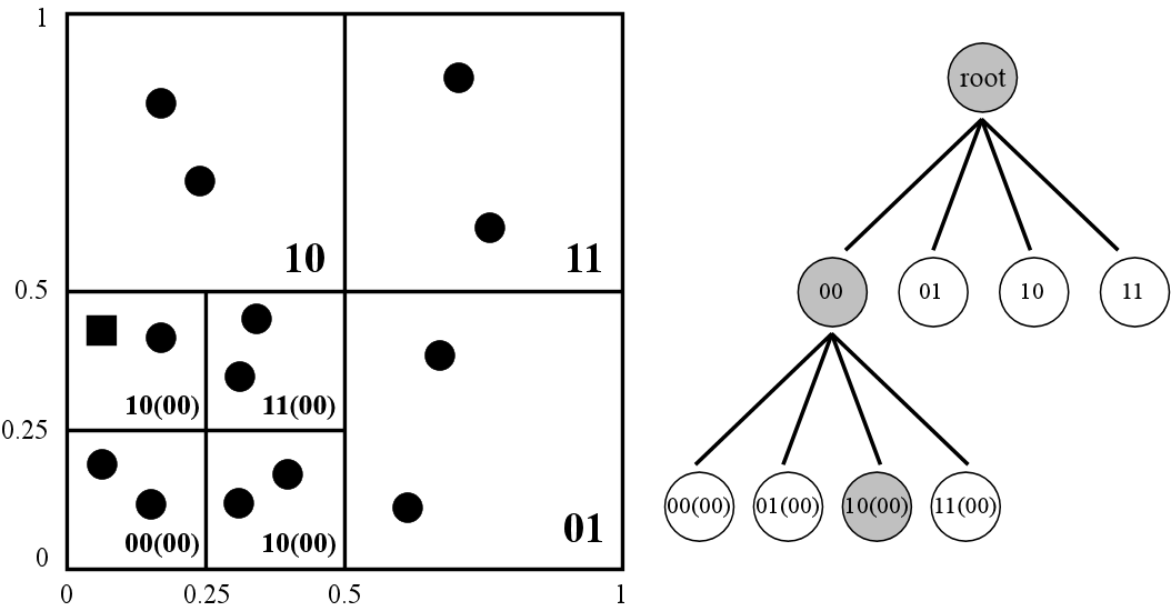
Figure 2: Looking for point $(x,y)=(0.1,0.425)$ (black square) on the quadtree; nodes traversed on the quadtree during the search are marked in grey. Quadrant number is indicated in two-bit Gray code; number in brackets indicate the number of the parent quadrant.

4.1 Algorithm 3 in practice

To illustrate the mechanics of Algorithm 3, we consider the classic geometric fractal, Maple Leaf, defined by $L=4$ functions $\phi_{i}$:

Example 4.1.

Maple Leaf:

$$\left\{\begin{array}[]{ll}\phi_{1}(x,y)=&(0.8x+0.1,0.8y+0.04)\\ \phi_{2}(x,y)=&(0.5x+0.25,0.5y+0.4)\\ \phi_{3}(x,y)=&(0.355x-0.355y+0.266,0.35x+0.355y+0.078)\\ \phi_{4}(x,y)=&(0.355x+0.355y+0.378,-0.355x+0.355y+0.434)\end{array}\right.$$

on the region $X=[0,1]^{2}$, with $p_{1}=0$, $p_{2}=-7$, $p_{3}=-3$ and $p_{4}=-7$.

Figure 3 shows the quadtrees placed over the image obtained from the points generated by Algorithm 3. In this example, we used $n_{\max}=64$. Since the number of points generated at the end of each iteration $i\geq 1$ is $4^{i}$, only after the fifth iteration there will be node divisions, as can be seen in the images. Note also that there may be points generated in an iteration that are already stored, hence the difference in the number of points after the tenth iteration ($1048534$) instead of the expected $4^{10}=1048576$.

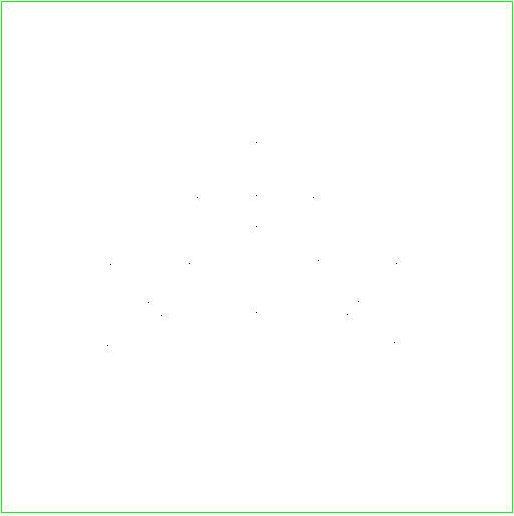
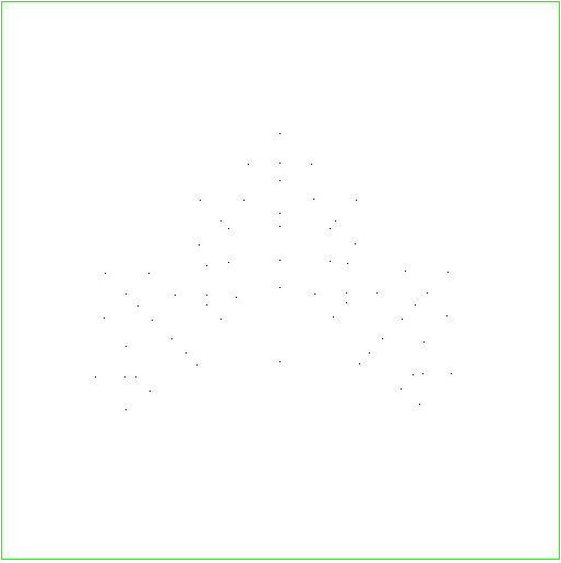
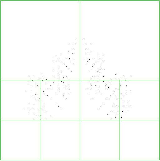
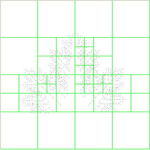
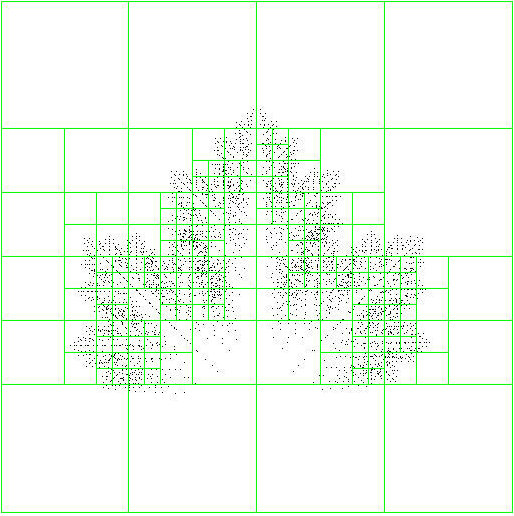
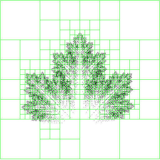
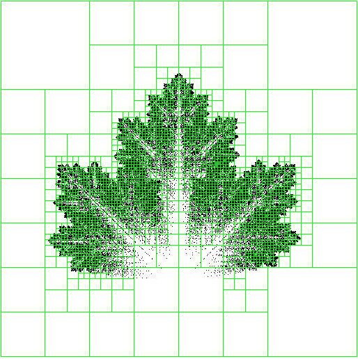
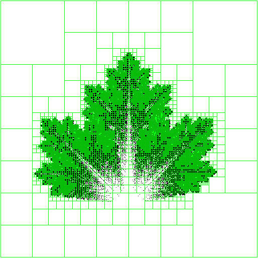
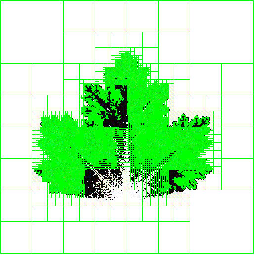
Figure 3: The quadtrees placed over the Maple Leaf fractal, $n_{\max}=64$: from top to bottom, left to right, the images ($512\times 512$ pixels) show the points generated from iteration $1$ ($n=4$ points) to $10$ ($n=1048534$ points).

To llustrate further, we consider an example with a different distribution of points across the region, showing in Figure 4 the quadtrees placed over the fractal.

Example 4.2.

This example is based on a very well-known fractal, the Barnsley Fern. It is defined by

$$\left\{\begin{array}[]{ll}\phi_{1}(x,y)=&(0.856x+0.0414y+0.07,-0.0205x+0.858y+0.147)\\ \phi_{2}(x,y)=&(0.244x-0.385y+0.393,0.176x+0.224y+0.102)\\ \phi_{3}(x,y)=&(-0.144x+0.39y+0.527,0.181x+0.259y-0.014)\\ \phi_{4}(x,y)=&(0.486,0.031x+0.216y+0.05)\end{array}\right.$$

on the region $X=[0,1]^{2}$, with $p_{1}=-11$, $p_{2}=-7$, $p_{3}=0$ and $p_{4}=0$.

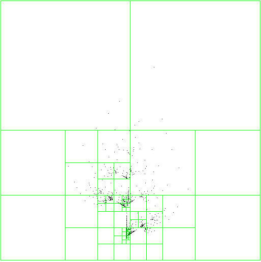
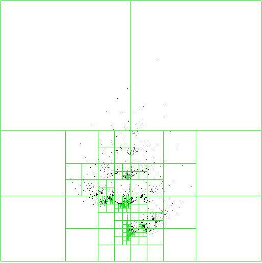
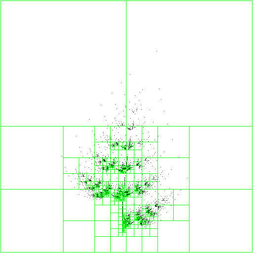
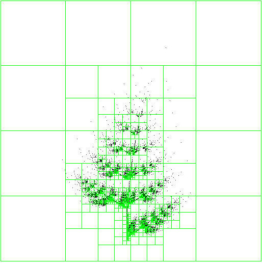
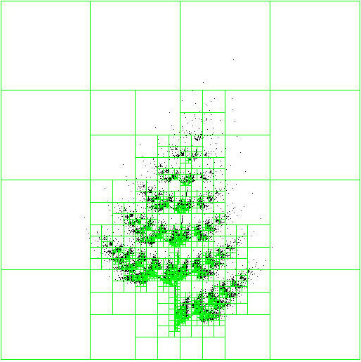
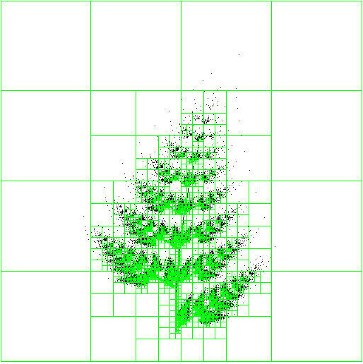
Figure 4: The quadtrees placed over the Barnsley Fern fractal, $n_{\max}=64$: from top to bottom, left to right, the images ($512\times 512$ pixels) show the points generated from iteration $1$ ($n=4$ points) to $10$ ($n=1014270$ points).

It should be clear from the previous discussion that $n_{\max}$ plays an important role in Algorithm 2. First, consider that this algorithm traverses the quadtree along a distinct path, visiting only the nodes computed by $Q(u,v)$, until reaching a leaf node (we remember that the height of a (quad)tree is the maximum distance of any node from the root). When this leaf node is visited, then a linear search for $(u,v)$ (of complexity $O\left(n_{\max}\right)$, line 11 of the algorithm) is made over the points on $D$ that are referred to by the node (indices of entries of $D$ stored on $I$). If $(u,v)$ is found, then $p$ is updated as in Algorithm 1.

If the linear search fails, then $(u,v)$ will be stored in $D$ and its index on $D$ is stored on $I$, if there are available entries on $I$; otherwise, the node is divided into four sons, the points assigned to it are distributed among its sons and Algorithm 2 is called recursively to store $(u,v)$ on one of its sons (which in itself may cause further node divisions).

If $n_{\max}$ is small then, for a given number $n$ of distinct points generated during an iteration (line 9 on Algorithm 3), there will be many subdivisions of the nodes on the quadtree, increasing its height, but the linear searches will make few comparison tests. Conversely, a larger $n_{\max}$ value reduces the height of the quadtree, but increases the cost of the linear search on a leaf node.

To ascertain the behaviour of Algorithm 3, we made a number of runs of our implementation written in Fortran 2003 compiled with gfortran 10.2.0 with -O3 optimization on a computer with an Intel Core i5-6400T 2.20 GHz processor and 6 GB of DDR3 RAM. The examples used were the Maple Leaf defined earlier and the Barnsley Fern.

Table 1 shows the quadtree height, $h$, at the end of $N=10$ iterations, and the execution time (in seconds) of our implementation of Algorithm 3. For the sake of comparison, we also present the execution time (in seconds) of our implementation of Algorithm 1, using a linear search. We note that the number of points generated after $10$ iterations was $n=1048534$ for the Maple Leaf and $n=1014270$ for the Barnsley Fern. It is evident from the data presented that, a) the use of the quadtree provides an execution time that is over $400$ times faster and b) there is an optimal value for $n_{\max}$, namely $64$, for which the least execution time was obtained, among the values used for $n_{\max}$.

Table 1: Maximum quadtree height and execution times of Algorithm 3.

	Algorithm 1	Algorithm 3
Example	Time [s]	$n_{\max}$	$h$	Time [s]
Maple Leaf	468.600	2	17	1.8610
		4	14	1.4590
		8	12	1.2660
		16	12	1.1920
		32	11	1.1120
		64	10	1.1000
		128	9	1.2200
		256	9	1.1730
		512	8	1.2900
		1024	8	1.5600
Barnsley Fern	483.479	2	26	2.3840
		4	25	1.7740
		8	24	1.4530
		16	23	1.2850
		32	22	1.2120
		64	21	1.1780
		128	20	1.1830
		256	19	1.2430
		512	17	1.4140
		1024	13	1.7570

Finally, to show an example of what we are actually interested in computing with IFSs, we present in Figure 5 the approximation of the attractor and the greyscale image representing the invariant measure for the Maple Leaf and Barnsley Fern idempotent IFSs. For more details, we refer the reader to (COS21, , Lemma 5.1).

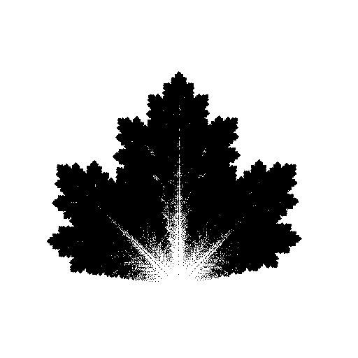
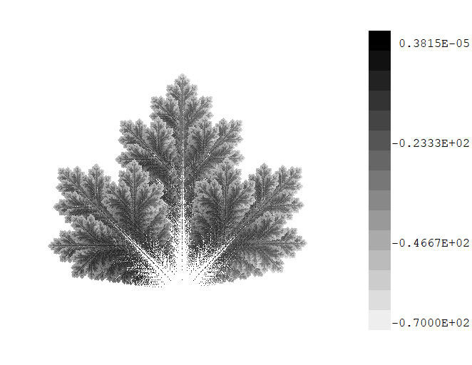
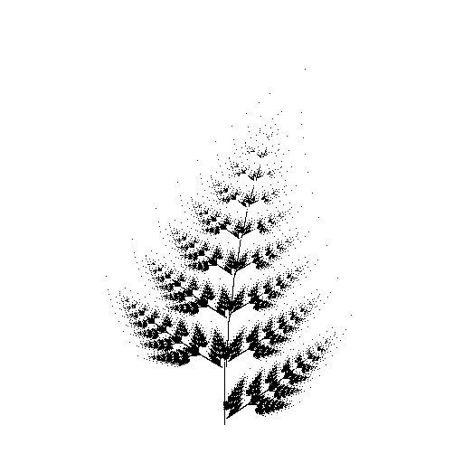
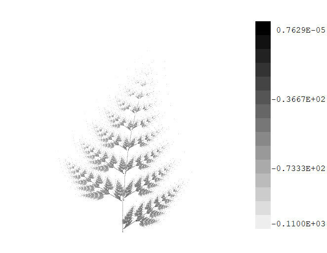
Figure 5: The approximation of the attractor and the greyscale representation of the invariant measure for the Maple Leaf (top) and Barnsley Fern (bottom) idempotent IFSs.

5 Complexity analysis of the deterministic IFS algorithms

To establish the complexity of Algorithm 1, we introduce the notation $n_{i}$, which is the number of points produced in each iteration, with $n_{0}=1$ (i.e. for the initial point). We assume that the search in line 15 of Algorithm 1 always fails, meaning that the searched-for point $(u,v)$ will always be stored in $T$ and therefore $n_{i-1}<n_{i}$ (that will give an upper-bound on the number of points generated at each iteration). Typically, one has sequences $n_{i}=L^{i}$.

Writing the expression for the total number of searches $S_{IFS}$ made in the algorithm, we obtain

$$S_{IFS}=\sum_{i=1}^{N}{\sum_{j=1}^{L}{\sum_{k=1}^{n_{i-1}}{f_{k}}}}$$ (14)

where $f_{k}$ is the number of comparison tests made on a search over a set of $n_{k}$ values. If a linear search is used, then $f_{k}\in O\left(n_{k}\right)$. In the worst case, $f_{k}=n_{k}$ and Equation (14) reduces to

$$S_{IFS}=-{\frac{N{L}^{2}}{L-1}}+\frac{L^{2}}{L-1}\sum_{i=1}^{N}{L^{L^{i-1}}}\simeq-{\frac{N{L}^{2}}{L-1}}+\frac{L^{2}}{L-1}L^{L^{N-1}}$$ (15)

where the summation is dropped since the term $L^{L^{N-1}}$ dominates the summation asymptotically as $N\rightarrow\infty$ and, therefore, $S_{IFS}\in O\left(L^{L^{N}}\right)$.

We note that the quadtree-based search has a complexity $O\left(n_{\max}\right)$. This is because the path traversed from the root to a leaf node during a search has at most length $h$ (there may be paths with shorter lengths, it depends on the distribution of points generated along the iterations - see Figure 3) and a linear search of at most $n_{\max}$ elements is carried out on a leaf node.

If we choose $n_{\max}=64$ and take $f(k)=n_{\max}$ in Equation (14), then Algorithm 3 has a total number of searches given as

$$S_{IFSq}=\frac{64\left({L}^{N+1}-L\right)}{L-1}\in O\left(L^{N}\right).$$ (16)

and, therefore,

$$S_{IFSq}\ll S_{IFS}.$$ (17)

6 Extension to Generalized IFS

The ideas presented in the previous sections extend naturally to Generalized IFSs. An algorithm to compute the attractor of a deterministic IFS is given in Algorithm 4, with a similar notation to that of Algorithm 1, and its version using a quadtree is given in Algorithm 5. They differ from the IFS algorithms in that the $\phi_{i}$ functions are now $\phi_{i}:\mathbb{R}^{4}\rightarrow\mathbb{R}^{2}$, $1\leq i\leq L$, and also that the set of points at each iteration is obtained by two nested loops of length $D.n$, leading to $(D.n)^{2}$ points being produced (at most); this is what makes GIFS costlier to compute than an IFS, since the number of generated points at each iteration grows much more rapidly.

Also, we note that the updates of $p$ on Algorithm 4, line 22 and on Algorithm 2, line 14 are made according to Equation (5) (for classic GIFS) and to Equation (9) (for idempotent GIFS).

Algorithm 4 Deterministic Algorithm for GIFS

1:function Deterministic_GIFS(input: $N,L,x,y,p$; output: $D$)

2:$N$, number of iterations

3:$L$, number of $\phi_{i}$ functions

4:$(x,y)$, coordinates of initial point

5:$p$, some property of the initial point

6:$D$, array of $(x,y,p)$ triplets Local: $T$, array of $(x,y,p)$ triplets

7:     $D.n\leftarrow 1$

8:     $D[D.n]\leftarrow(x,y,p)$

9:     for $i\leftarrow 1$ to $N$ do

10:         $T.n\leftarrow 0$ // initialize the number of triplets stored in $T$

11:         for $j\leftarrow 1$ to $L$ do

12:              for $k\leftarrow 1$ to $D.n$ do

13:                  for $l\leftarrow 1$ to $D.n$ do

14:                       $(u,v)\leftarrow\phi_{j}(D[k].x,D[k].y,D[l].x,D[l].y)$

15:                       initialize $r$ with some appropriate value

16:                       search for $(u,v)$ in $T$

17:                       if $(u,v)$ is not in $T$ then

18:                           $T.n\leftarrow T.n+1$

19:                           $T[T.n]\leftarrow(u,v,r)$

20:                       else

21:                           // $m$ is the index in $T$ such that $T[m].(x,y)=(u,v)$

22:                           update the value of $p$ in the triplet $T[m]$ (using $r$)

23:                       end if

24:                  end for

25:              end for

26:         end for

27:         $D\leftarrow T$

28:     end for

29:end function

Algorithm 5 Deterministic Algorithm for GIFS with quadtree-based search

1:function Deterministic_GIFS_quadtree(input: $N,L,x,y,p$; output: $D$)

2:$N$, number of iterations

3:$L$, number of $\phi_{i}$ functions

4:$(x,y)$, coordinates of initial point

5:$p$, some property of the initial point

6:$D$, array of $(x,y,p)$ triplets Local: $T$, array of $(x,y,p)$ triplets Local: $R$, root node of quadtree

7:     $D.n\leftarrow 1$

8:     $D[D.n]\leftarrow(x,y,p)$

9:     for $i\leftarrow 1$ to $N$ do

10:         $T.n\leftarrow 0$ // initialize the number of triplets stored in $T$

11:         create root node of quadtree, $R$

12:         for $j\leftarrow 1$ to $L$ do

13:              for $k\leftarrow 1$ to $D.n$ do

14:                  for $l\leftarrow 1$ to $D.n$ do

15:                       $(u,v)\leftarrow\phi_{j}(D[k].x,D[k].y,D[l].x,D[l].y)$

16:                       initialize $r$ with some appropriate value

17:                       Quadtree_Search_and_Insert($R,u,v,r,T$)

18:                  end for

19:              end for

20:         end for

21:         $D\leftarrow T$

22:     end for

23:end function

Once again, we will use two examples, defined below, to illustrate the functioning of the GIFS algorithms.

Example 6.1.

This example uses the GIFS $\mathcal{G}$ appearing in (JMS16, , Example 16). The IFS is defined by

$$\left\{\begin{array}[]{ll}\phi_{1}((x_{1},y_{1}),(x_{2},y_{2}))=&(0.25x_{1}+0.2y_{2},0.25y_{1}+0.2y_{2})\\ \phi_{2}((x_{1},y_{1}),(x_{2},y_{2}))=&(0.25x_{1}+0.2x_{2},0.25y_{1}+0.1y_{2}+0.5)\\ \phi_{3}((x_{1},y_{1}),(x_{2},y_{2}))=&(0.25x_{1}+0.1x_{2}+0.5,0.25y_{1}+0.2y_{2}))\end{array}\right.$$

on the region $X=[0,1]^{2}$, with $q_{1}=-2$, $q_{2}=0$ and $q_{3}=0$.

Example 6.2.

This example comes from (COS21, , Example 11.6). The IFS is defined by

$$\left\{\begin{array}[]{ll}\phi_{1}((x_{1},y_{1}),(x_{2},y_{2}))=&(0.2x_{1}+0.25x_{2}+0.04y_{2},0.16y_{1}-0.14x_{2}+0.20y_{2}+1.3)\\ \phi_{2}((x_{1},y_{1}),(x_{2},y_{2}))=&(0.2x_{1}-0.15y_{1}-0.21x_{2}+0.15y_{2}+1.3,\\ &0.25x_{1}+0.15y_{1}+0.25x_{2}+0.17)\\ \phi_{3}((x_{1},y_{1}),(x_{2},y_{2}))=&(0.355x_{1}+0.355y_{1}+0.378,\\ &-0.355x_{1}+0.355y_{1}+0.434-0.03y_{2})\end{array}\right.$$

on the region $X=[-0.1,2.1]^{2}$, with $q_{1}=-1$, $q_{2}=0$ and $q_{3}=-7$.

In Table 2 we present the execution times obtained with our Fortran 2003 implementations of Algorithm 4 and Algorithm 5. The number of points generated after $4$ iterations was $n=2011229$ for Example 6.1 and $n=13994321$ for Example 6.2.

Note that this enormous amount of points in the latter made us being unable to run Algorithm 4 in less than 12 hours of execution time, whereas with Algorithm 5 it is possible to quickly obtain a solution. Again, we notice that $n_{\max}=64$ provides the smallest execution time for both examples.

Table 2: Maximum quadtree height and execution times of Algorithm 5.

	Algorithm 4	Algorithm 5
Example	Time [s]	$n_{\max}$	$h$	Time [s]
6.1	3055.7301	2	27	5.3230
		4	27	3.8130
		8	17	3.3790
		16	14	3.1530
		32	12	3.0860
		64	11	3.0600
		128	11	3.4380
		256	10	3.5110
		512	9	4.1260
		1024	1	5.4640
6.2	N/A	2	26	155.6610
		4	25	19.0220
		8	24	16.1720
		16	23	13.6780
		32	22	13.1010
		64	21	12.7690
		128	20	13.8220
		256	19	14.3010
		512	17	16.4830
		1024	13	21.0930

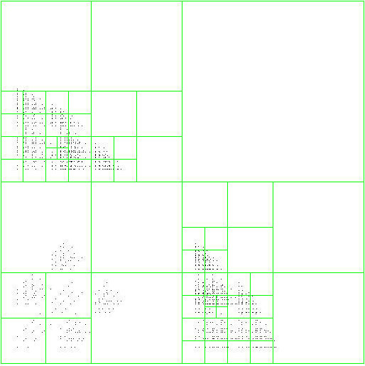
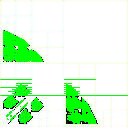
Figure 6: The quadtrees placed over the fractal for Example 6.1, $n_{\max}=64$: from top to bottom, left to right, the images ($512\times 512$ pixels) show the points generated from iteration $1$ ($n=3$ points) to $4$ ($n=2011229$ points).

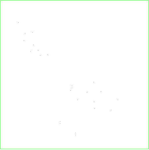
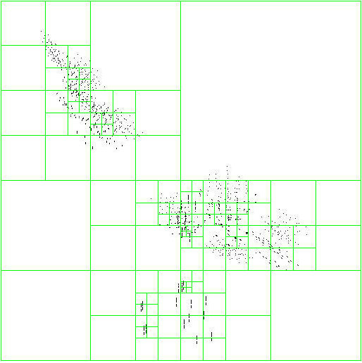
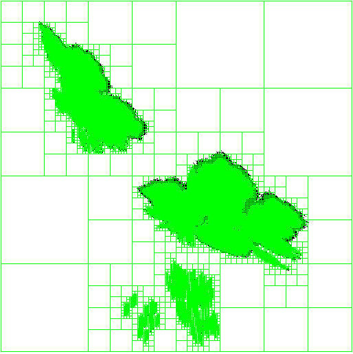
Figure 7: The quadtrees placed over the fractal for Example 6.2, $n_{\max}=64$: from top to bottom, left to right, the images ($512\times 512$ pixels) show the points generated from iteration $1$ ($n=3$ points) to $4$ ($n=13994321$ points).

As in Section 4.1, we present in Figure 8 the approximation of the attractor and the greyscale image representing the invariant measure for idempotent GIFSs.

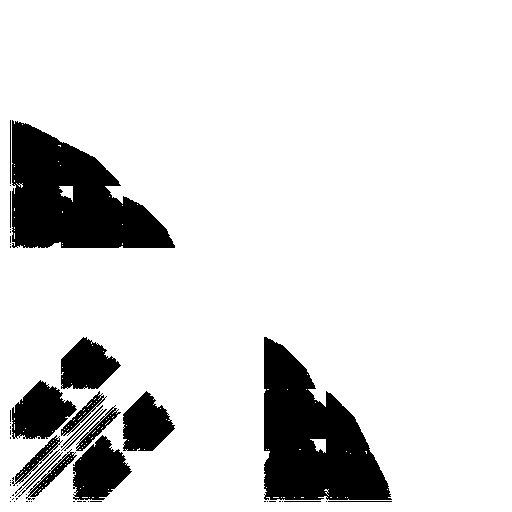
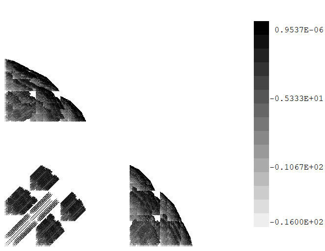
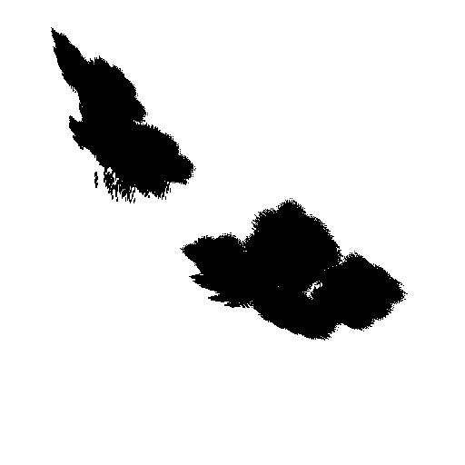
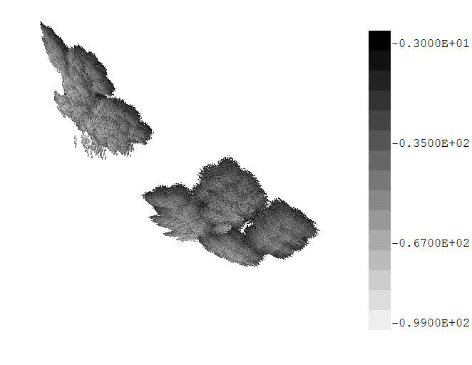
Figure 8: The approximation of the attractor and the greyscale representation of the invariant measure for Example 6.1 (top) and Example 6.2 (bottom) idempotent GIFSs.

6.1 Complexity analysis

Under the same hypotheses assumed for Algorithm 1, the total number of searches $S_{GIFS}$ made in Algorithm 4 is given by

$$S_{GIFS}=\sum_{i=1}^{N}{\sum_{j=1}^{L}{\sum_{k=1}^{n_{i-1}}{\sum_{l=1}^{n_{i-1}}{f_{k}}}}}$$ (18)

and, assuming linear searches are used, it reduces to

$$S_{GIFS}=\frac{L^{2}-L^{2}L^{N}}{(L-1)^{2}}+\frac{1}{L-1}\sum_{i=1}^{N}{L^{i+1}\,\left(L^{L^{i-1}}\right)}$$ (19)

and, since $L^{N+1}\,\left(L^{L^{N-1}}\right)$ dominates the summation, we may write

$$S_{GIFS}\simeq\frac{L^{2}-L^{2}L^{N}}{(L-1)^{2}}+\frac{1}{L-1}\left(L^{N+1}\,L^{L^{N-1}}\right)\in O\left(L^{L^{N}+N}\right).$$ (20)

For Algorithm 5, the total number of searches made, assuming $n_{\max}=64$ as before (see Section 5), is given by

$$S_{GIFSq}=\frac{64}{L^{2}-1}\left(\frac{\left(L^{2}\right)^{N+1}-L^{2}}{L}\right)\in O(L^{2N})$$ (21)

and, therefore,

$$S_{GIFSq}\ll S_{GIFS}.$$ (22)

7 Concluding remarks

We have presented a description of the deterministic algorithm used to compute approximations of invariant measures and its attractors for IFS and GIFS, as well as a quadtree-based search algorithm that allows the use of these (G)IFS in a reasonable running time. The results presented show that our approach is effective in turning the deterministic algorithms for G(IFS) tractable.

Funding

This research received no specific grant from any funding agency in the public, commercial, or not-for-profit sectors.

Conflict of interest

The authors declare that they have no conflict of interest.

References

- \bibcommenthead
- (1) Barnsley, M.F.: Fractals Everywhere. Academic Press, Inc., Boston, MA (1988)
- (2) Barnsley, M.F., Demko, S.G., Elton, J.H., Geronimo, J.S.: Invariant measures for Markov processes arising from iterated function systems with place-dependent probabilities. Ann. Inst. H. Poincaré Probab. Statist. 24(3), 367–394 (1988)
- (3) Jaros, P., Maślanka, Ł., Strobin, F.: Algorithms generating images of attractors of generalized iterated function systems. Numerical Algorithms 73(2), 477–499 (2016). https://doi.org/10.1007/s11075-016-0104-0
- (4) Galatolo, S., Nisoli, I.: An elementary approach to rigorous approximation of invariant measures. SIAM Journal on Applied Dynamical Systems 13(2), 958–985 (2014)
- (5) Galatolo, S., Monge, M., Nisoli, I.: Rigorous approximation of stationary measures and convergence to equilibrium for iterated function systems. Journal of Physics A: Mathematical and Theoretical 49(27), 274001 (2016). https://doi.org/10.1088/1751-8113/49/27/274001
- (6) da Cunha, R.D., Oliveira, E.R., Strobin, F.: A multiresolution algorithm to approximate the Hutchinson measure for IFS and GIFS. Communications in Nonlinear Science and Numerical Simulation 91, 105423 (2020). https://doi.org/10.1016/j.cnsns.2020.105423
- (7) Miculescu, R., Mihail, A., Urziceanu, S.-A.: A new algorithm that generates the image of the attractor of a generalized iterated function system. Numerical Algorithms 83(4), 1399–1413 (2020). https://doi.org/10.1007/s11075-019-00730-w
- (8) da Cunha, R.D., Oliveira, E.R., Strobin, F.: A multiresolution algorithm to generate images of generalized fuzzy fractal attractors. Numerical Algorithms 86(1), 223–256 (2021). https://doi.org/10.1007/s11075-020-00886-w
- (9) Finkel, R.A., Bentley, J.L.: Quad trees a data structure for retrieval on composite keys. Acta Informatica 4(1), 1–9 (1974). https://doi.org/10.1007/BF00288933
- (10) Samet, H.: The Quadtree and Related Hierarchical Data Structures. ACM Comput. Surv. 16(2), 187–260 (1984). https://doi.org/10.1145/356924.356930
- (11) Samet, H.: An Overview of Quadtrees, Octrees, and Related Hierarchical Data Structures. In: Earnshaw, R.A. (ed.) Theoretical Foundations of Computer Graphics and CAD, pp. 51–68. Springer, Berlin, Heidelberg (1988)
- (12) Har-peled, S.: Geometric Approximation Algorithms. American Mathematical Society, USA (2011)
- (13) Hutchinson, J.: Fractals and self-similarity. Indiana University Mathematics Journal 30(5), 713–747 (1981)
- (14) Mazurenko, N., Zarichnyi, M.: Invariant idempotent measures. Carpathian Math. Publ. 10(1), 172–178 (2018)
- (15) da Cunha, R.D., Oliveira, E.R., Strobin, F.: Fuzzy-set approach to invariant idempotent measures (2021)
- (16) Zarichnyi, M.M.: Spaces and maps of idempotent measures. Izv. Math. 74(3), 481–499 (2010)
- (17) Zaitov, A.A.: On a metric of the space of idempotent probability measures. Applied General Topology 21(1), 35–51 (2020). https://doi.org/10.4995/agt.2020.11865
- (18) Kolokoltsov, V.N., Maslov, V.P.: General form of endomorphisms in the space of continuous functions with values in a numerical commutative semiring (with the operation ). Dokl. Akad. Nauk SSSR 295(2), 283–287 (1987)
- (19) da Cunha, R.D., Oliveira, E.R., Strobin, F.: Existence of invariant idempotent measures by contractivity of idempotent Markov operators (2021)
- (20) Georgescu, F., Miculescu, R., Mihail, A.: Invariant measures of Markov operators associated to iterated function systems consisting of -max-contractions with probabilities. Indagationes Mathematicae 30(1), 214–226 (2019)
- (21) Miculescu, R.: Generalized Iterated Function Systems with Place Dependent Probabilities. Acta Applicandae Mathematicae 130(1), 135–150 (2014). https://doi.org/%****␣arxiv.tex␣Line␣1025␣****10.1007/s10440-013-9841-4
- (22) Mihail, A., Miculescu, R.: Generalized IFSs on noncompact spaces. Fixed Point Theory and Applications 2010(1), 584215 (2010). https://doi.org/10.1155/2010/584215
- (23) Mihail, A., Miculescu, R.: Applications of Fixed Point Theorems in the Theory of Generalized IFS. Fixed Point Theory and Applications 2008(1), 312876 (2008). https://doi.org/10.1155/2008/312876