Tightening geometric and dynamical constraints on dark energy and gravity:
galaxy clustering, intrinsic alignment and kinetic Sunyaev-Zel’dovich effect

Abstract

Conventionally, in galaxy surveys, cosmological constraints on the growth and expansion history of the universe have been obtained from the measurements of redshift-space distortions and baryon acoustic oscillations embedded in the large-scale galaxy density field. In this paper, we study how well one can improve the cosmological constraints from the combination of the galaxy density field with velocity and tidal fields, which are observed via the kinetic Sunyaev-Zel’dovich (kSZ) and galaxy intrinsic alignment (IA) effects, respectively. For illustration, we consider the deep galaxy survey by Subaru Prime Focus Spectrograph, whose survey footprint perfectly overlaps with the imaging survey of the Hyper Suprime-Cam and the CMB-S4 experiment. We find that adding the kSZ and IA effects significantly improves cosmological constraints, particularly when we adopt the non-flat cold dark matter model which allows both time variation of the dark energy equation-of-state and deviation of the gravity law from general relativity. Under this model, we achieve $31\%$ improvement for the growth index $\gamma$ and $>35\%$ improvement for other parameters except for the curvature parameter, compared to the case of the conventional galaxy-clustering-only analysis. As another example, we also consider the wide galaxy survey by the Euclid satellite, in which shapes of galaxies are noisier but the survey volume is much larger. We demonstrate that when the above model is adopted, the clustering analysis combined with kSZ and IA from the deep survey can achieve tighter cosmological constraints than the clustering-only analysis from the wide survey.

I Introduction

The baryon acoustic oscillations (BAO) Peebles and Yu (1970); Sunyaev and Zeldovich (1970); Eisenstein and Hu (1998) and redshift-space distortions (RSD) Peebles (1980); Kaiser (1987); Hamilton (1998) imprinted in large-scale galaxy distribution have been widely used as powerful tools to constrain the expansion and growth history of the Universe. Measurements of these signals enable galaxy clustering from redshift surveys to be one of the most promising probes to clarify the origin of the late-time cosmic acceleration, which could be explained by dark energy or modification of gravity Peacock et al. (2001); Tegmark et al. (2004); Eisenstein et al. (2005); Okumura et al. (2008); Guzzo et al. (2008); Weinberg et al. (2013); Aubourg et al. (2015); Okumura et al. (2016); Alam et al. (2017); Suyu et al. (2018); Alam et al. (2021). Upcoming spectroscopic galaxy surveys, including the Subaru Prime Focus Spectrograph (PFS) Takada et al. (2014), the Dark Energy Spectroscopic Instrument (DESI) DESI Collaboration et al. (2016), the Euclid space telescope Laureijs et al. (2011); Capak et al. (2019); Euclid Collaboration et al. (2020), and the Nancy Grace Roman Space Telescope Spergel et al. (2013a, b); Eifler et al. (2021), aim to constrain the dark energy equation-of-state and deviation of the gravitational law from general relativity (GR) with a precision at the sub-percent level.

In order to maximize the information encoded in the galaxy distribution in the large-scale structure (LSS) and to constrain cosmological parameters as tightly as possible, one needs to effectively utilize synergies between galaxy redshift surveys and other observations. In this respect, there is a growing interest of using two effects below as new probes of the LSS to improve cosmological constraints, complementary to the conventional galaxy clustering analysis. The first is the kinetic Sunyaev-Zel’dovich (kSZ) effect Sunyaev and Zeldovich (1980); Ostriker and Vishniac (1986), which can be observed via the measurement of cluster velocities by a synergy between galaxy surveys and cosmic microwave background (CMB) experiments. Theoretical and forecast studies suggest that kSZ measurements could provide robust tests of dark energy and modified gravity theories on large scales Hernández-Monteagudo et al. (2006); Okumura et al. (2014); Mueller et al. (2015); Sugiyama et al. (2016, 2017); Zheng (2020). The kSZ effect has been detected through the cross-correlations of CMB data with galaxy positions from various redshift surveys Hand et al. (2012); De Bernardis et al. (2017); Sugiyama et al. (2018); Planck Collaboration et al. (2018); Li et al. (2018); Calafut et al. (2021); Chaves-Montero et al. (2021); Chen et al. (2022).

The second probe is intrinsic alignment (IA) of galaxy shapes with the surrounding large-scale matter density field. The IA was originally proposed as a source of systematic effects on the measurement of the cosmological gravitational lensing Croft and Metzler (2000); Heavens et al. (2000); Lee and Pen (2000); Pen et al. (2000); Catelan et al. (2001); Jing (2002); Hirata and Seljak (2004); Heymans et al. (2004); Mandelbaum et al. (2006); Hirata et al. (2007); Okumura et al. (2009); Okumura and Jing (2009); Blazek et al. (2011); Singh et al. (2015). However, since the spatial correlation of IA follows the gravitational tidal field induced by the LSS, it contains valuable information and is considered as a cosmological probe complimentary to the galaxy clustering Schmidt and Jeong (2012); Faltenbacher et al. (2012); Chisari and Dvorkin (2013); Chisari et al. (2016); Okumura and Taruya (2020); Okumura et al. (2020); Taruya and Okumura (2020); Masaki et al. (2020); Akitsu et al. (2021a, b). Ongoing and future galaxy surveys focus on observing LSS at higher redshifts, $z>1$, at which the emission line galaxies (ELG) would be an ideal tracer of the LSS Laureijs et al. (2011); Takada et al. (2014); Tonegawa et al. (2015); Okada et al. (2016); Dawson et al. (2016); DESI Collaboration et al. (2016). Although IA has not yet been detected for ELG Mandelbaum et al. (2006, 2011); Tonegawa et al. (2018); Tonegawa and Okumura (2022), recent work Shi et al. (2021) has proposed an effective estimator to determine the IA of dark-matter halos using ELG, enhancing the signal-to-noise ratio at a statistically significant level. In any case, the accurate determination of galaxy shapes is of critical importance for IA to be a powerful tool to constrain cosmology. Thus, the synergy between imaging and spectroscopic surveys is essential because the accurate galaxy shapes and positions are determined from the former and latter, respectively.

In this paper, using the Fisher matrix formalism, we simultaneously analyze the velocity and tidal fields observed by the kSZ and IA effects, respectively, together with galaxy clustering. The combination of galaxy clustering with either IA or kSZ has been studied in earlier studies (e.g., Mueller et al., 2015; Sugiyama et al., 2017; Taruya and Okumura, 2020). This is the first joint analysis of these three probes and we want to see if cosmological constraints can be further improved by combining the combination. We emphasize that the question we want to address is not trivial at all because these probes utilize the information embedded in the same underlying matter fluctuations. Nevertheless, a key point is that these different probes suffer from different systematic effects, and can be in practice complementary to each other, thus used as a test for fundamental observational issues, such as the Hubble tension Verde et al. (2019), if the constraining power of each probe is similar. Furthermore, analyzing the kSZ and IA simultaneously enables us to study the correlation of galaxy orientations in phase space as proposed in our recent series of work Okumura et al. (2017, 2018, 2019); Okumura and Taruya (2020); Okumura et al. (2020). For our forecast, we mainly consider the PFS-like deep galaxy survey Takada et al. (2014) which overlaps with the imaging survey of the Hyper Suprime-Cam (HSC) Miyazaki et al. (2012); Aihara et al. (2018) and the CMB Stage-4 experiment (CMB-S4) Abazajian et al. (2016). To see how the cosmological gain by adding the IA and kSZ effects to galaxy clustering can be different for different survey geometries, we also analyze the Euclid-like wide galaxy survey Laureijs et al. (2011); Euclid Collaboration et al. (2020).

The rest of this paper is organized as follows. In section II we briefly summarize geometric and dynamic quantities to be constrained. Section III presents power spectra of galaxy density, velocity and ellipticity fields and their covariance matrix. We perform a Fisher matrix analysis and present forecast constraints in section IV, with some details further discussed in section V. Our conclusions are given in section VI. Appendix A describes the CMB prior used in this paper. In appendix B, we present conservative forecast constraints by restricting the analysis to large scales where linear perturbation theory is safely applied.

II Preliminaries

II.1 Distances

The comoving distance to a galaxy at redshift $z$, $\chi(z)$, is given by

$$\chi(z)=\int^{z}_{0}\frac{cdz^{\prime}}{H(z^{\prime})}\,,$$ (1)

with $c$ being the speed of light. The function $H(z)$ is the Hubble parameter which describes the expansion rate of the universe. Writing it as $H(z)=H_{0}E(z)$, we define the present-day value of the Hubble parameter by $H_{0}\equiv H(z=0)$, which is often characterized by the dimensionless Hubble constant, $h$, as $H_{0}=100\,h\,{\rm km~{}s}^{-1}{\rm Mpc}^{-1}$. Then the time-dependent function $E(z)$ is obtained from the Friedmann equation, and is expressed in terms of the (dimensionless) density parameters. In this paper, we consider the universe whose cosmic expansion is close to that in the standard cosmological model, with the dark energy having the time-varying equation of state. Allowing also the non-flat geometry, the function $E(z)$ is given by

$$E^{2}(z) = \Omega_{\rm m}(1+z)^{3}+\Omega_{K}(1+z)^{2}$$ (2)

$$+ \Omega_{\rm DE}(1+z)^{3(1+w_{0}+w_{a})}\exp{\left[-3w_{a}\frac{z}{1+z}\right]},$$

where $\Omega_{\rm m}$, $\Omega_{\rm DE}$ and $\Omega_{K}$ are the present-day energy density fractions of matter, dark energy and curvature, respectively, with $\Omega_{\rm m}+\Omega_{\rm DE}+\Omega_{K}=1$. In equation (2), the time-varying equation-of-state parameter for dark energy, denoted by $w(z)$, is assumed to be described by a commonly used and well tested parameterization Chevallier and Polarski (2001); Linder (2003):

$$w(z)=w_{0}+w_{a}\frac{z}{1+z}=w_{0}+w_{a}(1-a),$$ (3)

where $a=(1+z)^{-1}$ is the scale factor, and $w_{0}$ and $w_{a}$ characterize the constant part and the amplitude of time variation of the dark energy equation of state, respectively (see e.g., Ref. Colgáin et al. (2021), which studied how the different parameterization of $w(z)$ affects the constraining power of the deviation of a cosmological constant.)

The angular diameter distance, $D_{\rm A}(z)$, is given as

$$D_{\rm A}(z)=(1+z)^{-1}\frac{c}{H_{0}}S_{K}\left(\frac{\chi(z)}{c/H_{0}}\right),$$ (4)

where

$$S_{K}(x)=\left\{\begin{array}[]{lll}\sin{\left(\sqrt{-\Omega_{K}}x\right)}/\sqrt{-\Omega_{K}}&&\Omega_{K}<0,\\ x&&\Omega_{K}=0,\\ \sinh{\left(\sqrt{\Omega_{K}}x\right)}/\sqrt{\Omega_{K}}&&\Omega_{K}>0.\\ \end{array}\right.$$ (8)

Negative and positive values of $\Omega_{K}$ correspond to the closed and open universe, respectively. The geometric quantities, $D_{\rm A}(z)$ and $H(z)$, are the key quantities we directly constrain from the measurement of the BAO imprinted in the power spectra.

II.2 Perturbations

Density perturbations for a given component $i$ ($i=\{\rm m,g\}$ for matter and galaxies, respectively) are defined by the density contrast from the mean $\bar{\rho}_{i}(z)$,

$$\delta_{i}(\bm{x};z)\equiv\rho_{i}(\bm{x};z)/\bar{\rho}_{i}(z)-1.$$ (9)

Throughout the paper, we assume the linear relation for the galaxy bias with which the galaxy density fluctuation $\delta_{g}$ is related to the matter fluctuation $\delta_{m}$ through $\delta_{g}=b_{g}\,\delta_{m}$ Kaiser (1984). Then, an important quantity to characterize the evolution of the density perturbation is the growth rate parameter, defined as

$$f(z)=-\frac{d\ln D(z)}{d\ln(1+z)}=\frac{d\ln D(a)}{d\ln a},$$ (10)

where $D(z)$ is the linear growth factor of the matter perturbation, $D(z)=\delta_{m}(\bm{x};z)/\delta_{m}(\bm{x};0)$. The parameter $f$ quantifies the cosmological velocity field and the speed of structure growth, and thus is useful for testing a possible deviation of the gravity law from GR Guzzo et al. (2008). For this purpose, it is common to parameterize the $f$ parameter as

$$f(z)=\left[\Omega_{\rm m}(z)\right]^{\gamma},$$ (11)

where $\Omega_{\rm m}(z)=\Omega_{\rm m}(1+z)^{3}/E^{2}(z)$ is the time-dependent matter density parameter and the index $\gamma$ specifies a model of gravity, e.g., $\gamma\approx 6/11$ for the case of GR Peebles (1980); Linder (2005).

It is known that a class of modified gravity models exactly follows the same background evolution as in the $\Lambda$CDM model. However, the evolution of density perturbations can be different in general (see, e.g., Ref. Matsumoto et al. (2020) for degeneracies between the expansion and growth rates for various gravity models). Thus, it is crucial to simultaneously constrain the expansion and growth rate of the universe to distinguish between modified gravity models.

III Power spectra and the Fisher matrix

In this paper, we consider three cosmological probes observed in redshift space, i.e., density, velocity and ellipticity (tidal) fields. While nonlinearity of the density field has been extensively studied and a precision modeling of its redshift-space power spectrum has been developed (e.g., Peacock and Dodds, 1994; Scoccimarro, 2004; Taruya et al., 2010; Okumura et al., 2015), the understanding of the nonlinearities of velocity and tidal fields are relatively poor. However, there are several numerical and theoretical studies discussed beyond the linear theory, among which a systematic perturbative treatment has been also exploited (See, e.g., Refs. Okumura et al. (2014); Sugiyama et al. (2016, 2017) and Blazek et al. (2015, 2019); Vlah et al. (2020) for the nonlinear statistics of velocity and tidal fields, respectively). It is thus expected that a reliable theoretical template of their power spectra would be soon available, and an accessible range of their templates can reach, at least, at the weakly nonlinear regime. Hence, in our analysis, we consider the weakly nonlinear scales of $k\leq 0.2\,h\,{\rm Mpc}^{-1}$, as our default setup. Nevertheless, in order for a robust and conservative cosmological analysis, we do not use the shape information of the underlying matter power spectrum, which contains ample cosmological information but is more severely affected by the nonlinearities. That is, our focus in this paper is the measurements of BAO scales and RSD imprinted in the power spectra, and through the geometric and dynamical constraints on $D_{\rm A}(z)$, $H(z)$ and $f(z)$, we further consider cosmological constraints on models beyond the $\Lambda$ cold dark matter ($\Lambda$CDM) model. In appendix B, we perform a more conservative forecast by restricting th analysis to large scales, $k\leq 0.1\,h\,{\rm Mpc}^{-1}$, where linear perturbation theory predictions can be safely applied.

In what follows, we discuss how well one can maximize the cosmological information obtained from the BAO and RSD measurements, based on the linear theory predictions. While the linear-theory based template is no longer adequate at weakly nonlinear scales, the signal and information contained in the power spectrum can be in general maximized as long as we consider the Gaussian initial condition. In this respect, the results of our analysis presented below may be regarded as a theoretical upper bound on the cosmological information one can get. Furthermore, we assume a plane-parallel approximation for the cosmological probes Szalay et al. (1998); Szapudi (2004), taking the $z$-axis to be the line-of-sight direction. While properly taking into account the wide-angle effect provides additional cosmological constraints (see, e.g., Refs. Taruya et al. (2020), Castorina and White (2020); Shiraishi et al. (2020); Shiraishi et al. (2021a) and Shiraishi et al. (2021b) for the studies of the wide-angle effects on density, velocity and ellipticity fields, respectively), we leave the inclusion of this effect to our analysis as future work.

III.1 Density, velocity and ellipticity fields

In this subsection, based on the linear theory description, we write down the explicit relation between cosmological probes observed in redshift space to the matter density field. First, the density field of galaxies in redshift space, which we denote by $\delta_{g}^{S}$, is a direct observable in galaxy redshift surveys, and in Fourier space, it is related to the underlying density field of matter in real space on large scales, through $\delta_{g}^{S}(\bm{k};z)=K_{g}(\mu;z)\delta_{m}(\bm{k};z)$. The factor $K_{g}$ is the so-called linear Kaiser factor given by Kaiser (1987); Hamilton (1992); Okumura and Jing (2011),

$$K_{g}(\mu;z)=b_{g}(z)+f(z)\mu^{2},$$ (12)

where $b_{g}$ is the galaxy bias and $\mu$ is the directional cosine between the wavevector and line-of-sight direction, $\mu=\hat{\bm{k}}\cdot\hat{\bm{z}}$, with a hat denoting a unit vector. Note that setting $f$ to zero, the above equation is reduced to the Fourier counterpart of $\delta_{g}$ in equation (9).

Next, the cosmic velocity field is related to the density field through the continuity equation Fisher (1995); Strauss and Willick (1995). The observable through the kSZ effect is the line-of-sight component of the velocity, $v_{\parallel}$, and in linear theory, we have (in Fourier space) $v_{\parallel}(\bm{k};z)=if(z)\mu aH\delta_{m}(\bm{k};z)/k$. To be precise, the kSZ effect measures the temperature distortion of CMB, $\delta T$, detected at the position of foreground galaxies. It is explicitly written in Fourier space as $\delta T(\bm{k};z)=(T_{0}\tau/c)v_{\parallel}(\bm{k};z)=iK_{v}(\bm{k};z)\delta_{m}(k;z)$, where

$$K_{v}(k,\mu;z)=\frac{T_{0}\tau}{c}\frac{f(z)\mu aH(z)}{k}~{},$$ (13)

with $\tau$ being the optical depth. Since the distance to tracers of the velocity field is measured by redshift, the observed velocity field is affected by RSD, similarly to the density field in redshift space. Unlike the density field, however, the RSD contribution to the redshift-space velocity field appears at higher order Okumura et al. (2014). Thus, at leading order, the velocity field traced in redshift space coincides with that in real space in linearized theory, $v_{\parallel}^{S}=v_{\parallel}$. Note that the kSZ effect, which appears as secondary CMB anisotropies, is given by a line-of-sight integral of the velocity field, and thus the expression of Eq. (13) is just an approximation. We discuss the validity of this approximation in section V.3.

An alternative way to measure the velocity field $v_{\parallel}$ without observing the temperature distortion is to use velocity surveys, which enable us to uniquely constrain $f(z)$ Strauss and Willick (1995). We, however, do not consider observables from peculiar velocity surveys. The main reason is that these observations are limited to the nearby universe ($z\approx 0$) while we consider joint constraints with other probes from a single observation of the LSS. Thus, throughout this paper we refer the velocity field as the temperature distortion $\delta T$.

Table 1: Statistics and their abbreviations considered for given probes. Note that when two fields, $A$ and $B$, are considered, we use not only the auto-correlations ($P_{AA}$ and $P_{BB}$) but also the cross correlation, $P_{AB}$.

Probes	Statistics	Abbreviations	No. of	Parameters $\{\theta_{\alpha}\}$
			parameters $N_{\theta}$	nuisance	geometric/dynamical
Clustering	$P_{gg}$	$g$	4	$b\sigma_{8}$	$f\sigma_{8},H,D_{\rm A}$
kSZ	$P_{vv}$	$v$	4	$\tau$	$f\sigma_{8},H,D_{\rm A}$
IA	$P_{EE}$	$E$	3	$A_{\rm IA}$	$H,D_{\rm A}$
Clustering+IA	$P_{gg}+P_{EE}+P_{gE}$	$g+E$	5	$b\sigma_{8},A_{\rm IA}$	$f\sigma_{8},H,D_{\rm A}$
Clustering+kSZ	$P_{gg}+P_{vv}+P_{gv}$	$g+v$	5	$b\sigma_{8},\tau$	$f\sigma_{8},H,D_{\rm A}$
IA+kSZ	$P_{EE}+P_{vv}+P_{vE}$	$v+E$	5	$A_{\rm IA},\tau$	$f\sigma_{8},H,D_{\rm A}$
Clustering+IA+kSZ	$P_{gg}+P_{EE}+P_{vv}+P_{gE}+P_{gv}+P_{vE}$	$g+v+E$	6	$b\sigma_{8},A_{\rm IA},\tau$	$f\sigma_{8},H,D_{\rm A}$

Finally, we use ellipticities of galaxies as a tracer of the tidal field. The two-component ellipticity of galaxies is defined as

$$\gamma_{(+,\times)}(\bm{x};z)=\frac{1-q}{1+q}\left(\cos{(2\phi_{x})},\sin{(2\phi_{x})}\right),$$ (14)

where $\phi_{x}$ is the position angle of the major axis relative to the reference axis, defined on the plane normal to the line-of-sight direction, and $q$ is the minor-to-major axis ratio of a galaxy shape. We set $q$ to zero for simplicity Okumura et al. (2009). As a tracer of LSS, a leading-order description of the ellipticity field is to relate $\gamma_{(+,\times)}$ linearly to the tidal gravitational field, known as the linear alignment (LA) model Catelan et al. (2001); Hirata and Seljak (2004); Okumura et al. (2019); Okumura and Taruya (2020). In Fourier space, this is given by

$$\gamma_{(+,\times)}(\bm{k};z)=b_{K}(z)\left(k_{x}^{2}-k_{y}^{2},2k_{x}k_{y}\right)\frac{\delta_{m}(\bm{k};z)}{k^{2}}.$$ (15)

Just like the velocity field, the ellipticity field is not affected by RSD in linear theory Okumura and Taruya (2020). We then define E-/B-modes, $\gamma_{(E,B)}$, which are the rotation-invariant decomposition of the ellipticity field Crittenden et al. (2002),

$$\gamma_{E}(\bm{k};z)+i\gamma_{B}(\bm{k};z)=e^{-2i\phi_{k}}\left\{\gamma_{+}(\bm{k};z)+i\gamma_{\times}(\bm{k};z)\right\},$$ (16)

where $\phi_{k}$ is the azimuthal angle of the wavevector projected on the celestial sphere (Note that $\phi_{k}$ has nothing to do with the directional cosine of the wavevector, and thus $\phi_{k}\neq\cos^{-1}{\mu}$). By writing $\gamma_{(E,B)}(\bm{k};z)=K_{(E,B)}(\mu;z)\delta_{m}(\bm{k};z)$, we have $K_{B}=0$ and

$$K_{E}(\mu;z)=b_{K}(z)(1-\mu^{2}).$$ (17)

In Eq. (15) or (16), the parameter $b_{K}$ quantifies the response of individual galaxy shapes to the tidal field of LSS, and it is conventionally characterized by introducing the parameter $A_{\rm IA}$ as follows (e.g., Schmitz et al., 2018; Kurita et al., 2021):

$$b_{K}(z)=0.01344A_{\rm IA}(z)\Omega_{\rm m}/D(z).$$ (18)

Note that the parameter $A_{\rm IA}$ generally depends on properties of the given galaxy population as well as redshift. The analysis of numerical simulations, however, demonstrated that for fixed galaxy/halo properties, $A_{\rm IA}$ is nearly redshift-independent Kurita et al. (2021). We thus treat $A_{\rm IA}$ as a constant throughout this paper.

III.2 Linear power spectra of the three fields

As summarized in the previous subsection, the three cosmological fields, i.e. density, velocity and ellipticity, are related to the matter field linearly through the coefficients, $K_{g}$, $K_{v}$ and $K_{E}$, respectively. Provided their explicit expressions, we can analytically compute the auto-power spectra of these fields and their cross-power spectra. There are in total six power spectra measured in redshift space, each of which exhibits anisotropies characterized by the $\mu$ dependence Ballinger et al. (1996); Seo and Eisenstein (2003); Matsubara (2004); Okumura and Taruya (2020). Writing these spectra as $P_{ij}(\bm{k};z)=P_{ij}(k,\mu;z)$ with $i,j=\{g,v,E\}$, they are expressed in a concise form as,

$$P_{ij}(k,\mu;z) =K_{i}(k,\mu;z)K_{j}(k,\mu;z)P_{\rm lin}(k;z),$$ (19)

where $P_{\rm lin}(k;z)$ is the linear power spectrum of matter fluctuation in real space. The normalization of the density fluctuation is characterized by the $\sigma_{8}$ parameter, defined by the linear RMS density fluctuation within a sphere of radius $8h^{-1}$Mpc, and thus $P_{\rm lin}(k;z)\propto\sigma_{8}^{2}(z)$. While each of the three auto-power spectra, $P_{gg}$, $P_{vv}$ and $P_{EE}$, can be measured from each of the three individual probes, namely galaxy clustering, kSZ and IA, respectively, the cross-power spectra become measurable only when two probes are simultaneously made available. Particularly, the correlation between velocity and ellipticity fields, $P_{vE}$, has been proposed recently by our earlier studies and it can be probed by the joint analysis of the kSZ (or peculiar velocities) and IA effects Okumura et al. (2017, 2018, 2019); Okumura and Taruya (2020); Okumura et al. (2020); van Gemeren and Chisari (2020). Table 1 summarizes all the statistics used in this paper.

To measure the power spectra, the observed galaxy positions measured with redshift and angular position need to be converted into the comoving positions by introducing a reference cosmology, with a help of equations (1) and (4). An apparent mismatch between the reference and true cosmology causes a geometric distortion in the measured power spectra, which is yet another anisotropy known as the Alcock-Paczynski (AP) effect Alcock and Paczynski (1979). This AP effect has been extensively investigated for the galaxy power spectrum in redshift space Ballinger et al. (1996); Matsubara and Suto (1996); Seo and Eisenstein (2003); Blazek et al. (2014). The AP effect on the kSZ and IA statistics has been studied relatively recently by Refs. Sugiyama et al. (2017) and Taruya and Okumura (2020), respectively. In all of the six power spectra, $P_{ij}$, their observable counterpart $P_{ij}^{\rm obs}$ are related to the true ones through the relation,

$$P_{ij}^{{\rm obs}}\left(k_{\perp}^{\rm fid},k_{\parallel}^{{\rm fid}};z\right)=\frac{H(z)}{H^{\rm fid}(z)}\left\{\frac{D_{\rm A}^{\rm fid}(z)}{D_{\rm A}(z)}\right\}^{2}P_{ij}\left(k_{\perp},k_{\parallel};z\right),$$ (20)

where $k_{\perp}$ and $k_{\parallel}$ are the wavenumber perpendicular and parallel to the line of sight, $(k_{\perp},k_{\parallel})=k(\sqrt{1-\mu^{2}},\mu)$. The quantities $D_{\rm A}^{\rm fid}(z)$ and $H^{\rm fid}(z)$ are the angular diameter distance and expansion rate computed from fiducial cosmological parameters in the reference cosmology, and $k_{\parallel}^{\rm fid}=k_{\parallel}H^{\rm fid}(z)/H(z)$ and $k_{\perp}^{\rm fid}=k_{\perp}\,D_{\rm A}(z)/D_{\rm A}^{\rm fid}(z)$. The prefactor $\frac{H(z)}{H^{\rm fid}(z)}\left\{\frac{D_{\rm A}^{\rm fid}(z)}{D_{\rm A}(z)}\right\}^{2}$ accounts for the difference in the cosmic volume in different cosmologies.

As formulated above, $K_{g}$, $K_{v}$ and $K_{E}$ respectively contain two $(b,f)$, two $(\tau,f)$, and one $(A_{\rm IA})$ parameters, and all the power spectra depend on $(H,D_{\rm A})$ through the AP effect (see table 1). Thus, we have six parameters in total, $\theta_{\alpha}=(b\sigma_{8},A_{\rm IA}\sigma_{8},\tau,f\sigma_{8},H,D_{\rm A})$, among which the first three are nuisance parameters that we want to marginalize over. The latter three parameters carry the cosmological information which characterize the growth of structure and geometric distances, and are determined by measuring the anisotropies in the power spectra.

III.3 Covariance matrix

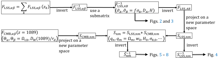
Figure 1: Flowchart of our Fisher matrix analysis from dynamical and geometric constraints to cosmological parameter constraints. The Fisher matrices of the LSS probes, namely galaxy clustering, IA and kSZ, are given for each redshift bin $z_{k}$ at the upper left. The Fisher matrix from the CMB prior is given at the lower left.

Writing all the power spectra obtained from the galaxy clustering, kSZ and IA as
$P_{a}=(P_{gg},P_{EE},P_{vv},P_{gE},P_{gv},P_{vE})$, we will below examine several forecast analysis with a different number of power spectra, which we denote by $N_{P}$. Specifically, depending on how many probes are simultaneously available, we consider seven possible cases with $N_{P}=1$, $3$ or $6$, summarized in table 1. Correspondingly, the covariance matrix ${\rm Cov}_{ab}$ becomes a $N_{P}\times N_{P}$ matrix, defined as ${\rm Cov}_{ab}(k,\mu;z)=\left\langle P_{a}P_{b}\right\rangle-\left\langle P_{a}\right\rangle\left\langle P_{b}\right\rangle$, for a given wavevector, ${\bf k}=(k,\mu)$. The full $6\times 6$ Gaussian covariance matrix reads

$${\rm Cov}_{ab}(k,\mu;z)=\left[\begin{array}[]{cccccc}2\{\widetilde{P}_{gg}\}^{2}&2\{P_{gE}\}^{2}&2\{P_{gv}\}^{2}&2\widetilde{P}_{gg}P_{gE}&2\widetilde{P}_{gg}P_{gv}&2P_{gv}P_{gE}\\ 2\{P_{gE}\}^{2}&2\{\widetilde{P}_{EE}\}^{2}&2\{P_{vE}\}^{2}&2P_{gE}\widetilde{P}_{EE}&2P_{gE}P_{vE}&2\widetilde{P}_{EE}P_{vE}\\ 2\{P_{gv}\}^{2}&2\{P_{vE}\}^{2}&2\{\widetilde{P}_{vv}\}^{2}&2P_{gv}P_{vE}&2\widetilde{P}_{vv}P_{gv}&2P_{vE}\widetilde{P}_{vv}\\ 2\widetilde{P}_{gg}P_{gE}&2P_{gE}\widetilde{P}_{EE}&2P_{gv}P_{vE}&\widetilde{P}_{gg}\widetilde{P}_{EE}+\{P_{gE}\}^{2}&\widetilde{P}_{gg}P_{vE}+P_{gE}P_{gv}&P_{gv}\widetilde{P}_{EE}+P_{gE}P_{vE}\\ 2\widetilde{P}_{gg}P_{gv}&2P_{gE}P_{vE}&2\widetilde{P}_{vv}P_{gv}&\widetilde{P}_{gg}P_{vE}+P_{gE}P_{gv}&\widetilde{P}_{gg}\widetilde{P}_{vv}+\{P_{gv}\}^{2}&P_{gE}\widetilde{P}_{vv}+P_{gv}P_{vE}\\ 2P_{gv}P_{gE}&2\widetilde{P}_{EE}P_{vE}&2P_{vE}\widetilde{P}_{vv}&P_{gv}\widetilde{P}_{EE}+P_{gE}P_{vE}&P_{gE}\widetilde{P}_{vv}+P_{gv}P_{vE}&\widetilde{P}_{EE}\widetilde{P}_{vv}+\{P_{vE}\}^{2}\\ \end{array}\right]~{},$$ (27)

where $\widetilde{P}_{ii}=\widetilde{P}_{ii}(k,\mu;z)$ denotes an auto-power spectrum ($i=\{g,v,E\}$) including the shot noise. Assuming the Poisson shot noise, we have

$$\widetilde{P}_{gg}=P_{gg}+\frac{1}{n_{g}},$$ (28)

$$\widetilde{P}_{vv}=P_{vv}+\left(1+R_{N}^{2}\right)\left(\frac{T_{0}\tau}{c}\right)^{2}\frac{(faH\sigma_{d})^{2}}{n_{v}},$$ (29)

$$\widetilde{P}_{EE}=P_{EE}+\frac{\sigma_{\gamma}^{2}}{n_{\gamma}},$$ (30)

where the quantities $n_{g}$, $n_{v}$ and $n_{\gamma}$ are the number density of the galaxies obtained from galaxy clustering, kSZ and IA observations, respectively. Though different notations are explicitly used for these three samples, $n_{g}=n_{v}=n_{\gamma}$ when one considers a single galaxy population for the analysis. When one uses a single galaxy population as a tracer of the density, velocity and ellipticity fields, there should be a shot noise contribution in the cross correlations. Such a noise term, however, vanishes because $\langle v_{\parallel}\rangle=0$ Sugiyama et al. (2017) and $\langle\gamma_{E}\rangle=0$ Taruya and Okumura (2020).

In the shot noise terms of $P_{vv}$ and $P_{EE}$, there appear factors $\sigma_{d}=\sqrt{\langle v_{\parallel}^{2}\rangle}$ and $\sigma_{\gamma}=\sqrt{\langle\gamma_{E}^{2}\rangle}$, which respectively represent the velocity dispersion and shape noise of galaxies, respectively. Using perturbation theory, $\sigma_{d}$ can be evaluated as

$$\sigma_{d}^{2}=\frac{1}{3}\int\frac{d^{3}q}{(2\pi)^{3}}\frac{P_{\theta\theta}(q;z)}{q^{2}}=\frac{1}{6\pi^{2}}\int dqP_{\theta\theta}(q;z),$$ (31)

where $P_{\theta\theta}$ is the power spectrum of velocity divergence. In the limit of linear theory, we have $P_{\theta\theta}=P_{{\rm lin}}$, and in the standard cosmological model, it is predicted to give $aH\sigma_{d,{\rm lin}}\simeq 600D(z)~{}{\rm km}/{\rm s}$ Vlah et al. (2012), and hence $faH\sigma_{d,{\rm lin}}\simeq 600f(z)D(z)\approx 300~{}{\rm km}/{\rm s}$ over the redshift considered in this work. Finally, the parameter $R_{N}$ is the inverse signal-to-noise ratio of the kSZ temperature fluctuations Sugiyama et al. (2017). The rms noise for the kSZ measurement of the CMB-S4 experiment is $\left\langle\delta T\right\rangle\sim 2\mu K$, leading to $R_{N}\sim 10$ Sugiyama et al. (2017).

Note that considering only the Gaussian contribution of the covariance matrix (equation (27)) may underestimate the statistical errors. Particularly, the kSZ effect generally suffers from a correlated non-Gaussian noise due to the residual foreground contamination, e.g., cosmic infrared background and thermal SZ effect (see e.g., Bobin et al., 2014; Planck Collaboration et al., 2018). Though our focus is on relatively large scales and we adopt the Gaussian covariance, such non-Gaussian contributions need to be taken into account for a more realistic forecast study.

III.4 Fisher matrix formalism

To quantify the constraining power for the dynamical and geometric parameters above and cosmological parameters, we use the Fisher matrix formalism. Although forecast studies with the Fisher matrix have been widely performed in cosmology, there is a limited number of relevant works that consider the kSZ and IA observations to constrain cosmology, specifically through the RSD and AP effect. One is the paper by Sugiyama, Okumura & Spergel Sugiyama et al. (2017), who discussed a benefit of using kSZ observations. Another paper is Taruya & Okumura Taruya and Okumura (2020), who demonstrated that combining galaxy clustering with IA observations is beneficial and improves geometric and dynamical constraints. The present paper complements these two previous works, and further put forward the forecast study by combining all three probes.

Given a set of parameters to be estimated, $\{\theta_{\alpha}\}$, where $\alpha=1,\cdots,N_{\theta}$, and provided a set of observed power spectra $\{P_{a}\}$, the Fisher matrix is evaluated with

$$F_{\alpha\beta}= \frac{V_{s}}{4\pi^{2}}\int^{k_{\rm max}}_{k_{\rm min}}dkk^{2}\int^{1}_{-1}d\mu$$

$$\times\sum_{a,b=1}^{N_{P}}\frac{\partial P_{a}(k,\mu)}{\partial\theta_{\alpha}}\left[{\rm Cov}^{-1}\right]_{ab}\frac{\partial P_{b}(k,\mu)}{\partial\theta_{\beta}},$$ (32)

where $V_{s}$ is the comoving survey volume for a given redshift range, $z_{\min}\leq z\leq z_{\max}$, and $k_{\rm min}$ and $k_{\rm max}$ are respectively the minimum and maximum wavenumbers used for cosmological data analysis, the former of which is specified with the survey volume by $k_{\rm min}=2\pi/V_{s}^{1/3}$. Note that for the analysis using a single probe ($N_{P}=1$), namely when we consider either of $P_{gg}$, $P_{EE}$ or $P_{vv}$, the covariance matrix ${\rm Cov}_{ab}$ is reduced to the power spectrum squared (see equation (27)).

Provided the Fisher matrix, the expected errors on the parameters of interest, marginalizing over other parameters, are computed by inverting the Fisher matrix and constructing the $\overline{N}_{\vartheta}\times\overline{N}_{\vartheta}$ submatrix $\overline{\bm{F}}$; for example, when one wants to evaluate the two-dimensional error contours for a specific pair of parameters, $\vartheta_{A}\in\,\theta_{\alpha}$ $(A=1,2)$, the $2\times 2$ submatrix is constructed with $C_{AB}\equiv[\overline{\bm{F}}]^{-1}_{AB}$ $(A,B=1,2)$. Also, the one-dimensional marginalized error on a parameter $\vartheta_{A}$ is obtained from $\sigma_{A}^{2}\equiv[\overline{\bm{F}}]^{-1}_{AA}$ (see, e.g., Ref. Seo and Eisenstein (2003) for details).

Although our original Fisher matrix is given for the parameters $\{\theta_{\alpha}\}$ determined from the AP effect and RSD, the model-independent geometric and dynamical constraints are translated into specific cosmological model constraints by projecting the matrix into a new parameter space of interest,

$$S_{nm}=\sum_{\alpha,\beta}^{N_{\theta}}\frac{\partial\theta_{\alpha}}{\partial q_{n}}F_{\alpha\beta}\frac{\partial\theta_{\beta}}{\partial q_{m}},$$ (33)

where $\{q_{n}\}$ is the set of parameters in the new parameter space ($n=1,\cdots,N_{q}$), i.e., non-flat $w_{0}w_{a}\gamma$ CDM model and others in our case (see section IV.2), and $\bm{S}$ is thus a $N_{q}\times N_{q}$ matrix. Once again, the uncertainties of the parameters can be obtained by taking the submatrix, e.g., $C_{AB}\equiv[\overline{\bm{S}}]^{-1}_{AB}$, $\sigma_{A}^{2}\equiv[\overline{\bm{S}}]^{-1}_{AA}$, etc.

For a further discussion on the performance of the constraining power on multiple parameters, we compute the Figure-of-merit (FoM) defined by

$${\rm FoM}=\left\{{\rm det}(\overline{\bm{F}})\right\}^{1/\overline{N}_{\vartheta}},\ \ \ \ \ \ \ {\rm FoM}=\left\{{\rm det}(\overline{\bm{S}})\right\}^{1/\overline{N}_{\varrho}},$$ (34)

where quantities with the bar, $\overline{\bm{F}}$ and $\overline{\bm{S}}$, denote $\overline{N}_{\vartheta}\times\overline{N}_{\vartheta}$ and $\overline{N}_{\varrho}\times\overline{N}_{\varrho}$ submatrices of $\bm{F}$ and $\bm{S}$ ($\overline{N}_{\vartheta}<N_{\theta},\overline{N}_{\varrho}<N_{q}$), respectively, constructed through the inversion described above. In the definition provided in Ref. Albrecht et al. (2006), $\overline{N}_{\vartheta}=\overline{N}_{\varrho}=2$ and the obtained FoM describes the inverse of the area of the error contour in the marginalized parameter plane for two parameters. Here, the FoM is defined for an arbitrary number of parameters, and the obtained value corresponds to a mean radius of the $\overline{N}_{\vartheta}$ (or $\overline{N}_{\varrho}$) dimensional volume of the errors.

Table 2: Expected volume, number density and bias of emission line galaxies for given redshift ranges, $z_{\min}\leq z\leq z_{\max}$ of the deep (PFS-like) survey, taken from Ref. Takada et al. (2014).

Redshift		Volume $V_{s}$	$10^{4}n$	Bias
$z_{\rm min}$	$z_{\rm max}$	($h^{-3}{\rm Gpc}^{3}$)	$(h^{3}{\rm Mpc}^{-3})$	$b_{g}$
0.6	0.8	$0.59$	$1.9$	$1.18$
0.8	1.0	$0.79$	$6.0$	$1.26$
1.0	1.2	$0.96$	$5.8$	$1.34$
1.2	1.4	$1.09$	$7.8$	$1.42$
1.4	1.6	$1.19$	$5.5$	$1.50$
1.6	2.0	$2.58$	$3.1$	$1.62$
2.0	2.4	$2.71$	$2.7$	$1.78$

IV Results

In this section, we present geometric and dynamical constraints on cosmological parameters based on the Fisher matrix analysis of galaxy clustering, IA and kSZ effects. In figure 1, we summarizes the steps of the analysis of this section graphically, motivated by figure 2 of Ref. Seo and Eisenstein (2003).

IV.1 Setup

To jointly analyze the galaxy clustering, IA and kSZ, we need to use data from galaxy surveys and CMB experiments: positions and shapes of galaxies are respectively used to quantify clustering and IA from a galaxy survey, while the velocity field is inferred by observing the CMB temperature distortion at the angular position of each galaxy.

Table 3: Same as table 2 but for the wide (Euclid-like) survey, taken from Ref. Euclid Collaboration et al. (2020).

Redshift		Volume $V_{s}$	$10^{4}n$	Bias
$z_{\rm min}$	$z_{\rm max}$	($h^{-3}{\rm Gpc}^{3}$)	$(h^{3}{\rm Mpc}^{-3})$	$b_{g}$
0.9	1.1	$7.94$	$6.86$	$1.46$
1.1	1.3	$9.15$	$5.58$	$1.61$
1.3	1.5	$10.05$	$4.21$	$1.75$
1.5	1.8	$16.22$	$2.61$	$1.90$

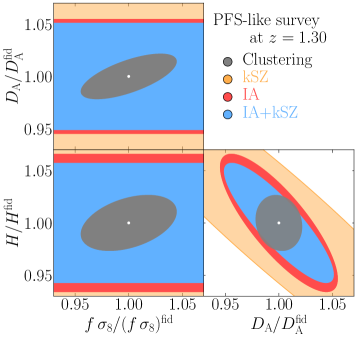
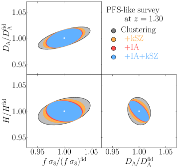
Figure 2: Two-dimensional $1\sigma$ error contours on the geometric distances, $D_{\rm A}(z)$ and $H(z)$, and the linear growth rate $f(z)\sigma_{8}(z)$, expected from the wide (PFS-like) survey. Since there are seven redshift bins, we here show the result for the central redshift bin, $1.2<z<1.4$, as an example. Left panel: Constraints from each of the clustering, kSZ and IA, and the combination of the latter two. Right panel: Similar to the left panel but joint constraints from the combination of kSZ, IA and galaxy clustering. Note that the joint constraints obtained from clustering and IA (red contours) almost overlap with those from clustering, IA and kSZ (blue contours).

As we mentioned in section I, there are a number of planned spectroscopic galaxy surveys aiming at constraining cosmology with a high precision. These surveys are generally categorized into the two types: (narrow but) deep surveys and (shallow but) wide surveys. In the Fisher matrix analysis below, we consider the Subaru PFS and Euclid as examples of deep and wide surveys, respectively, both of which target emission line galaxies (ELG) as a tracer of the LSS. Tables 2 and 3 show the redshift range, survey volume, and number density and bias of the ELG samples for the PFS Takada et al. (2014) and Euclid Euclid Collaboration et al. (2020), respectively. Ref. Shi et al. (2021) has proposed an estimator to directly detect IA of host halos using the observation of the ELGs. In the forecast analysis presented below, we consider that the power spectra related to the IA are measured with this estimator. Following the result of Ref. Shi et al. (2021), we set the fiducial value of the IA amplitude to $A_{\rm IA}=18$, assuming its redshift independence. The PFS galaxy sample provides high-quality shape information thanks to the imaging survey of the HSC Miyazaki et al. (2012); Aihara et al. (2018), and we thus set the shape noise, $\sigma_{\gamma}$, to $\sigma_{\gamma}=0.2$ for the deep survey Hikage et al. (2019). For the wide survey, following Ref. Euclid Collaboration et al. (2020), we set it to $\sigma_{\gamma}=0.3$. We will discuss the effect of changing the fiducial values of $A_{\rm IA}$ and $\sigma_{\gamma}$ in section V.

Similarly to the forecast study of the kSZ effect in Ref. Sugiyama et al. (2017), we consider CMB-S4 Abazajian et al. (2016) as a CMB experiment for the expected observation of the kSZ effect. While the angular area of the PFS is completely overlapped with that of the CMB-S4, the half of the Euclid area is covered by the CMB-S4 Euclid Collaboration et al. (2022). Thus, when considering the statistics related to the kSZ effect, namely $P_{vv}$, $P_{gv}$ and $P_{vE}$, in the wide survey, the elements of the covariance matrix for these statistics are multiplied by two. Furthermore, the values of $k_{\min}$ for these terms become larger by the factor of $2^{1/3}$. We choose $R_{\rm N}=10$ as our fiducial choice, following Ref. Sugiyama et al. (2017). For the velocity dispersion, we use the liner theory value as a fiducial value, $\sigma_{v}=\sigma_{v,{\rm lin}}$. The combination of $(1+R_{\rm N}^{2})\sigma_{v}^{2}$ contributes to the shot noise of the kSZ power spectrum. We will test the effect of these choices in section V.

In the following analysis, we assume the spatially flat $\Lambda$CDM model as our fiducial model Planck Collaboration et al. (2016a): $\Omega_{\rm m}=1-\Omega_{\rm DE}=0.315$, $\Omega_{K}=0$, $w_{0}=-1$, $w_{a}=0$, $H_{0}=67.3~{}[{\rm km/s/Mpc}]$ and the present-day value of $\sigma_{8}$, $\sigma_{8,0}\equiv\sigma_{8}(z=0)$, to be $\sigma_{8,0}=0.8309$. For computation of the linear power spectrum in equation (19), $P_{\rm lin}(k;z)$, we use the publicly-available CAMB code Lewis et al. (2000). When we consider the model which allows deviation of the structure growth from GR prediction, we set the fiducial value of $\gamma$ in equation (11) to be consistent with GR, $\gamma=0.545$.

Finally, the maximum wavenumber of the power spectra used for the cosmological analysis with the Fisher matrix is set to $k_{\rm max}=0.2\,h$ Mpc^-1. While forecast results with this choice, presented below as our main results, give tight geometrical and dynamical constraints, we also consider in Appendix B a conservative choice of $k_{\rm max}=0.1\,h\,{\rm Mpc}^{-1}$, and discuss its impact on the parameter constraints.

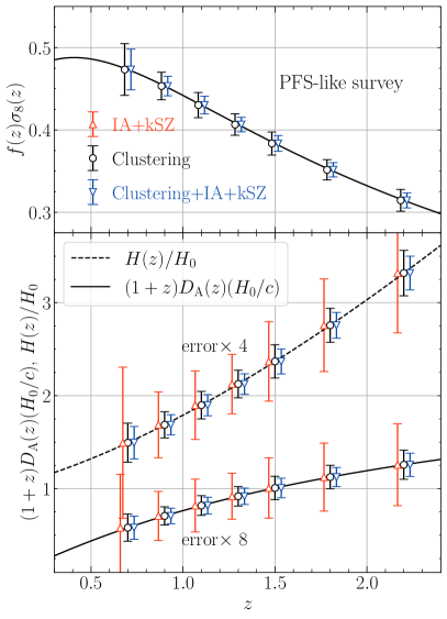
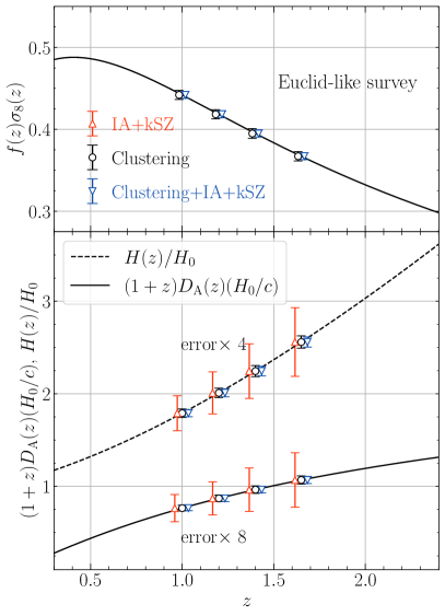
Figure 3: Left set: one-dimensional marginalized errors on the growth rate $f(z)\sigma_{8}(z)$ (upper panel) and geometric distances (lower panel), $D_{A}(z)$ and $H(z)$, expected from the deep (PFS-like) survey. Right set: same as the left set but the result expected from wide (Euclid-like) survey. The errors on $H$ and $D_{\rm A}$ are multiplied by 4 and 8, respectively, for illustration.

IV.2 Geometric and dynamical constraints

Let us first look at model-independent dynamical and geometric constraints, namely the constraints on $f(z)\sigma_{8}(z)$, $D_{\rm A}(z)$ and $H(z)$, expected from the upcoming Subaru PFS survey. From the original Fisher matrix which includes these parameters in addition to nuisance parameters, as summarized in table 1, we obtain the marginalized constraints as described in section III.4.

The left panel of figure 2 shows the two-dimensional $1\sigma$ error contours on $f\sigma_{8}$, $D_{\rm A}$ and $H$ normalized by their fiducial values, which are obtained individually from galaxy clustering ($P_{gg}$), kSZ ($P_{vv}$) and IA ($P_{EE}$). Since the PFS is a deep survey and has seven redshift bins at $0.6<z<2.4$ (see Table 2), we here plot the result for the central redshift bin, $1.2<z<1.4$, where the number density of galaxies is the largest. Note that the left panel of figure 2 does not consider any cross correlation between different probes, namely $P_{gE}$, $P_{gv}$ and $P_{vE}$ (see table 1). As clearly shown in the figure, using either $P_{EE}$ or $P_{vv}$ cannot constrain the growth rate. This is because the intrinsic galaxy shapes themselves are insensitive to RSD in linear theory and the kSZ only constrains the combination of $f\sigma_{8}$ and $\tau$ without imposing any prior on $\tau$. Nevertheless, each single measurement of kSZ and IA can give meaningful constraints on $D_{\rm A}$ and $H$. Then, including the cross correlation, the combination of the two probes, namely $P_{vv}$ and $P_{EE}$ as well as $P_{vE}$, improves the constraint on $(D_{\rm A},H)$, depicted as the blue contour.

Interestingly, the constraining power on $D_{\rm A}$ and $H$, when combining kSZ and IA, can become tighter, and for the one-dimensional marginalized error, the precision on each parameter achieves a few percent level. Although the galaxy clustering still outperforms the kSZ and IA observations, systematic effects in each probe come to play differently (e.g., galaxy bias, shape noises and optical depth), and in this respect, the geometric constraints from the kSZ and IA are complementary as alternatives to those from the galaxy clustering. Thus, constraining the geometric distances with kSZ and/or IA effects would help addressing recent systematics-related issues such as the Hubble tension.

The right panel of figure 2 shows the result similar to the left panel, but the joint constraints combining kSZ and/or IA with galaxy clustering. Compared to the results from the single probe, the constraints are indeed improved, as previously demonstrated in Refs. Sugiyama et al. (2017) (clustering+kSZ) and Taruya and Okumura (2020) (clustering+IA). Here we newly show that the combination of all three probes, characterized by the six power spectra, can further tighten the constraints on both the geometric distances and growth of structure. The results imply that adding any of these power spectra can extract independent cosmological information even though they measure the same underlying matter field. The left panel of figure 3 summarizes the one-dimensional marginalized errors on $f\sigma_{8}$, $D_{\rm A}$ and $H$ expected from the deep (PFS-like) survey, plotted as a function of $z$ over $0.6<z<2.4$. Over all redshifts studied here, adding the information from kSZ and IA measurements does improve the geometric and dynamical constraints.

Table 4: Summary of the cosmological models investigated in the forecast study.

Model	No. of free	Parameters $\{q_{n}\}$			CMB prior	Result
	parameters $N_{q}$	Flat	Non-flat	MG		(Fig.)
$w_{0}$ flat	4	$\Omega_{\rm m},H_{0},w_{0},\sigma_{8}$	$-$	$-$	$-$	4
$w_{0}w_{a}$ flat	5	$\Omega_{\rm m},H_{0},w_{0},w_{a},\sigma_{8}$	$-$	$-$	Yes	5
$w_{0}w_{a}$ non-flat	6	$\Omega_{\rm m},H_{0},w_{0},w_{a},\sigma_{8}$	$\Omega_{K}$	$-$	Yes	6
$w_{0}w_{a}\gamma$ flat	6	$\Omega_{\rm m},H_{0},w_{0},w_{a},\sigma_{8}$	$-$	$\gamma$	Yes	7
$w_{0}w_{a}\gamma$ non-flat	7	$\Omega_{\rm m},H_{0},w_{0},w_{a},\sigma_{8}$	$\Omega_{K}$	$\gamma$	Yes	8

IV.3 Cosmological parameter constraints

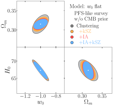
Figure 4: Cosmological constraints on the $w_{0}$ flat model expected from the deep (PFS-like) survey without relying on the CMB prior. In each panel, contours show the $1\sigma$ confidence levels, with the amplitude parameter today, $\sigma_{8,0}=\sigma_{8}(0)$, marginalized over. Note that the joint constraints obtained from clustering and IA (red contours) are almost entirely behind those from clustering, IA and kSZ (blue contours).

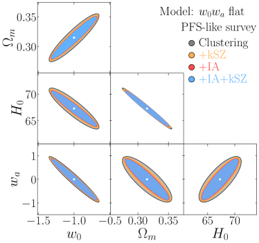
Figure 5: Cosmological constraints on the $w_{0}w_{a}$ flat model expected from the deep (PFS-like) survey. Unlike figure 4, CMB prior information is added here. In each panel, contours show the $1\sigma$ confidence levels, with the amplitude parameter today, $\sigma_{8,0}=\sigma_{8}(0)$, marginalized over. The joint constraints obtained from clustering and IA (red contours) are almost entirely behind those from clustering, IA and kSZ (blue contours).

Provided the model-independent geometric and dynamical constraints estimated from the original Fisher matrix in section IV.2, we further discuss specific cosmological model constraints listed in Table 4. In what follows, except the $w_{0}$ flat CDM model, we add the CMB prior information to constrain cosmological parameters and follow the conventional approach adopted in the data analysis of BOSS Eisenstein et al. (2005); Percival et al. (2007); Beutler et al. (2017), which do not use the information of the full-shape power spectra. To be precise, we introduce the following scaling parameters:

$$\alpha_{\parallel}=\frac{H(z)r_{d}}{H^{\rm fid}(z)r_{d}^{\rm fid}},\ \ \ \ \ \ \alpha_{\perp}=\frac{D_{\rm A}(z)r_{d}^{\rm fid}}{D_{\rm A}^{{\rm fid}}(z)r_{d}},$$ (35)

where the quantity $r_{d}$ is the sound horizon scale at the drag epoch $z_{d}$ when photons and baryons are decoupled Eisenstein and Hu (1998), given by

$$r_{d}=\int^{\infty}_{z_{d}}\frac{c_{s}(z)}{H(z)}dz,$$ (36)

with $c_{s}$ being the sound speed in the photon-baryon fluid. We then redefine the fiducial wavenumbers $k_{\parallel}$ and $k_{\perp}$, which appear in Eq. (20), as $k_{\parallel}^{\rm fid}=k_{\parallel}/\alpha_{\parallel}$ and $k_{\perp}^{\rm fid}=k_{\perp}\alpha_{\perp}$. With this parameterization, the original expression for the power spectrum at Eq. (20), taking the AP effect into account, is recast as

$$P_{ij}^{{\rm obs}}\left(k_{\perp}^{\rm fid},k_{\parallel}^{{\rm fid}};z\right)=\left(\frac{r_{d}^{\rm fid}}{r_{d}}\right)^{3}\frac{\alpha_{\parallel}}{\alpha_{\perp}^{2}}P_{ij}\left(k_{\perp},k_{\parallel};z\right),$$ (37)

where the prefactor $(r_{d}^{\rm fid}/r_{d})^{3}(\alpha_{\parallel}/\alpha_{\perp}^{2})$ is equivalent to that in equation (20). Note that the dimensionless quantities $r_{d}/D_{\rm A}$ and $Hr_{d}$ are related to the actual BAO scales measurable from galaxy surveys, i.e., angular separation and redshift width of the acoustic scales. In this respect, with the form given in equation (37), we are assuming that the main contribution to the AP effect comes from the BAO. As discussed in Ref. Beutler et al. (2017), the uncertainty on the $r_{d}$ measurement from the Planck experiment is only at the level of $\sim 0.2$ per cent Planck Collaboration et al. (2016a) and fixing $r_{d}$ in equation (37) has a negligible effect on our cosmological parameter estimation. Based on this argument, we approximately set the pre-factor $(r_{d}^{\rm fid}/r_{d})^{3}$ to unity for the Fisher matrix analysis below.

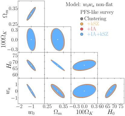
Figure 6: Same as figure 5 but for the $w_{0}w_{a}$ non-flat model.

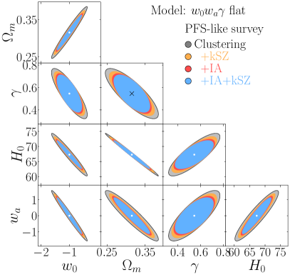
Figure 7: Same as figure 5 but for the $w_{0}w_{a}\gamma$ flat model.

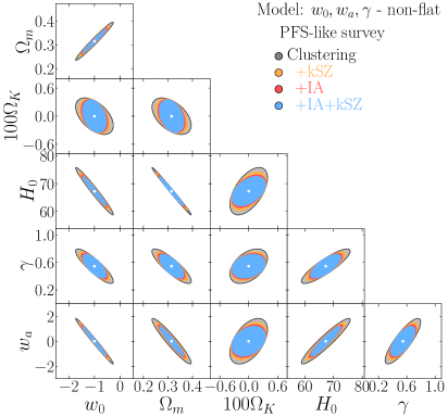
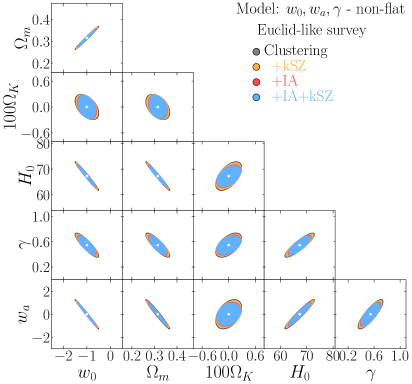
Figure 8: Top: Same as figure 5 but for the $w_{0}w_{a}\gamma$ non-flat model from the deep (PFS-like) survey. Bottom: Similar to the top panel but from the wide (Euclid-like) survey.

Table 5: Fractional marginalized errors on cosmological parameters, $\sigma/\theta^{\rm fid}$, for the four specific models. The CMB prior information is added for all the results here. Since the fiducial values of $w_{a}$ and $\Omega_{K}$ are zero, we show the absolute errors, $\sigma$. Since the absolute errors on $\Omega_{K}$ are small, we show the errors multiplied by 100.

			Deep (PFS-like) survey					Wide (Euclid-like) survey
			Clustering					Clustering
Model	$\sigma/\theta^{\rm fid}$		only	+kSZ	+IA	+IA+kSZ		only	+kSZ	+IA	+IA+kSZ
$w_{0},w_{a}$	$\Omega_{\rm m}$		0.0850	0.0813	0.0765	0.0746		0.0590	0.0578	0.0559	0.0555
flat	$w_{0}$		0.230	0.224	0.213	0.208		0.164	0.163	0.157	0.156
	$w_{a}$		0.638	0.613	0.584	0.569		0.455	0.450	0.438	0.434
	$H_{0}$		0.0383	0.0363	0.0338	0.0329		0.0257	0.0251	0.0241	0.0239
$w_{0},w_{a}$	$\Omega_{\rm m}$		0.0877	0.0841	0.0788	0.0767		0.0592	0.0580	0.0561	0.0556
non-flat	$w_{0}$		0.240	0.232	0.220	0.214		0.164	0.163	0.157	0.156
	$w_{a}$		0.665	0.634	0.600	0.583		0.457	0.452	0.440	0.437
	$H_{0}$		0.0415	0.0397	0.0370	0.0360		0.0262	0.0256	0.0247	0.0244
	$100\Omega_{K}$		0.231	0.229	0.223	0.222		0.162	0.161	0.161	0.161
$w_{0},w_{a},\gamma$	$\Omega_{\rm m}$		0.1459	0.1244	0.1075	0.0990		0.1004	0.0955	0.0840	0.0804
flat	$w_{0}$		0.415	0.359	0.314	0.288		0.288	0.272	0.245	0.234
	$w_{a}$		1.036	0.907	0.804	0.743		0.761	0.715	0.655	0.625
	$H_{0}$		0.0691	0.0585	0.0501	0.0458		0.0452	0.0429	0.0374	0.0358
	$\gamma$		0.271	0.238	0.217	0.202		0.193	0.182	0.169	0.161
$w_{0},w_{a},\gamma$	$\Omega_{\rm m}$		0.1679	0.1380	0.1162	0.1055		0.1114	0.1039	0.0884	0.0836
non-flat	$w_{0}$		0.484	0.400	0.340	0.307		0.330	0.304	0.264	0.248
	$w_{a}$		1.202	1.004	0.865	0.786		0.841	0.774	0.686	0.646
	$H_{0}$		0.0833	0.0682	0.0571	0.0516		0.0548	0.0510	0.0430	0.0404
	$100\Omega_{K}$		0.258	0.245	0.234	0.230		0.194	0.189	0.182	0.179
	$\gamma$		0.304	0.256	0.228	0.210		0.231	0.212	0.191	0.179

Now, the model-independent parameters in our original Fisher matrix, combining all three probes, become $\theta_{\alpha}=(b\sigma_{8},A_{\rm IA}\sigma_{8},\tau,f\sigma_{8},\alpha_{\parallel},\alpha_{\perp})$, and the marginalized constraints on $\vartheta_{A}=(f\sigma_{8},\alpha_{\perp},\alpha_{\parallel})$ are evaluated for each $z$-slice by constructing the $3\times 3$ sub-matrix $\overline{\bm{F}}_{\rm LSS}(z_{k})$. Summing up these sub-matrices over all the redshift bins, i.e., $\overline{\bm{F}}_{{\rm LSS}}=\sum_{k}\overline{\bm{F}}_{{\rm LSS}}(z_{k})$, we project it into a new parameter space to test the model-dependent cosmological parameters $q_{n}$ through equation (33). The most general model considered in our analysis is the $w_{0}w_{a}\gamma$ non-flat model, with $q_{n}=(\Omega_{\rm m},w_{0},w_{a},H_{0},\Omega_{K},\gamma,\sigma_{8,0})$. All the cosmological models we consider in this paper are summarized in table 4.

Let us show our main results for the deep, PFS-like survey below. Figures 4 – 7 and the top panel of figure 8 plot the expected two-dimensional constraints on pairs of model parameters for different cosmological models. Also, table 5 and figure 9 summarize the one-dimensional marginalized constraints. We will discuss all the results in detail in the rest of this subsection. Except for figure 4, all the following results are obtained adding the CMB prior information, as detailed in Appendix A. Thus, the constraints are obtained from the combination of the Fisher matrices of the LSS and CMB, $\bm{S}=\bm{S}_{\rm LSS}+\bm{S}_{\rm CMB}$. For all cases, the nuisance parameters characterizing the power spectrum normalization on each probe namely $b\sigma_{8}$, $\tau$, and $A_{\rm IA}\sigma_{8}$, are marginalized over. Comparisons of the obtained constraints with those from the wide, Euclid-like survey will be presented in section V.1.

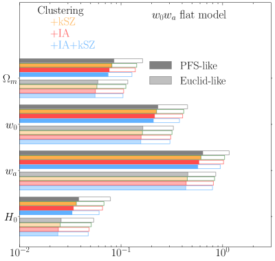
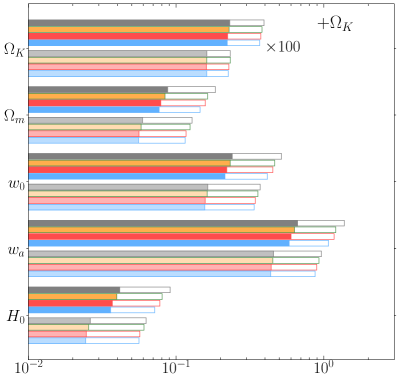
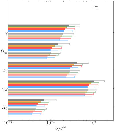
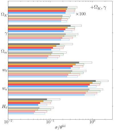
Figure 9: Marginalized $1\sigma$ errors on cosmological parameters, relative to their corresponding fiducial values, $\sigma/\theta^{\rm fid}$. The darkly and lightly filled bars show the errors from the deep (PFS-like) and wide (Euclid-like) surveys, respectively. The top-left and top-right panels are for the $w_{0}w_{a}$ flat and non-flat models, respectively. Similarly, the bottom-left and bottom-right panels are for $w_{0}w_{a}\gamma$ flat and non-flat models, respectively. The CMB prior information is added for all the results here. Since the fiducial values of $w_{a}$ and $\Omega_{K}$ are zero, we show the absolute errors, $\sigma$. Since the absolute errors on $\Omega_{K}$ are small, we show the errors multiplied by 100. The hollow bars are similar with the filled bars but based on the conservative analysis with the scales of $k\leq 0.1\,h\,{\rm Mpc}^{-1}$ (see appendix B).

Figure 4 shows the case for the $w_{0}$ flat model, in which we vary $q_{n}=(\Omega_{m},w_{0},H_{0},\sigma_{8,0})$. Only for this model, we do not add the CMB prior and use LSS probes as our primary data set. As shown in Ref. Taruya and Okumura (2020), adding IA to galaxy clustering significantly improves the constraints. If the kSZ measurement is added, one can achieve a similar (but slightly weaker) improvement. Simultaneously analyzing galaxy clustering with kSZ and IA, the constraint on each cosmological parameter gets even tighter, by $15-21\%$, compared to the clustering-only constraints.

In figure 5, adding the CMB prior information, we show an extension of the parameter space by allowing the time-varying dark energy equation-of-state, which is the $w_{0}w_{a}$ flat model described by the parameters $q_{n}=(\Omega_{\rm m},w_{0},w_{a},H_{0},\sigma_{8,0})$. Here, the improvement by adding IA is not so significant compared to the former case, due mainly to a dominant contribution from the CMB prior, consistent with the result of Ref.  Taruya and Okumura (2020). However, combining the galaxy clustering with both kSZ and IA measurements, we can improve the constraints further, for example, on $w_{a}$ by $\sim 11\%$, as shown in table 5 and figure 9. Figure 6 examines the case with non-zero $\Omega_{K}$, by introducing another degree of freedom in the parameter space on top of the $w_{0}w_{a}$ flat model. Note that based on the BAO experiments at high $z$, a best achievable precision on $\Omega_{K}$, limited by the cosmic variance, has been studied in detail in Ref. Takada and Doré (2015). In our forecast, the spatial curvature has already been tightly constrained by the CMB prior. Thus, the resulting constraints are similar with those of the model with $\Omega_{K}=0$ in figure 5.

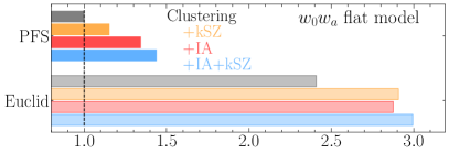
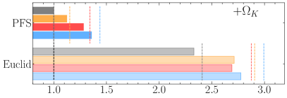
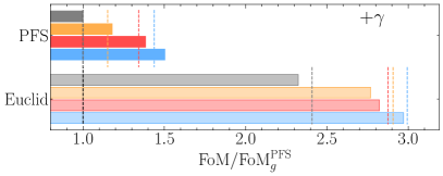
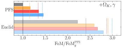
Figure 10: FoM of cosmological impact for clustering only (gray), clustering $+$ kSZ (yellow), clustering $+$ IA (red) and clustering $+$ IA $+$ kSZ (blue). The upper-left and upper-right panels are the results for the $w_{0}w_{a}$ flat and non-flat models, respectively. Similarly, the lower-left and lower-right panels are the results for the $w_{0}w_{a}\gamma$ flat and non-flat models, respectively. The CMB prior information is added for all the results here. In each panel, the values of FoM are normalized by that for the PFS survey with clustering-only analysis. The yellow, red and blue vertical lines indicate the FoM values obtained in the upper-left panel for comparison.

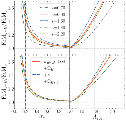
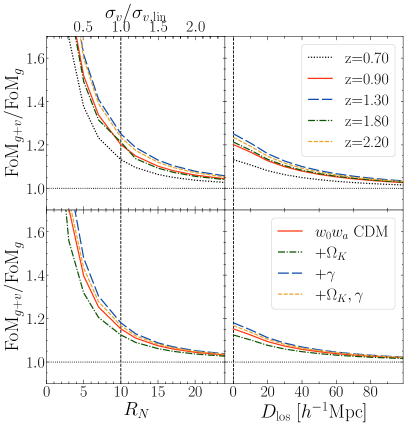
Figure 11: Relative impact of combining IA (left set) and kSZ (right set) on the parameter constraints, defined by the ratio of figure-of-merit, ${\rm FoM}_{g+E}/{\rm FoM}_{g}$ and ${\rm FoM}_{g+v}/{\rm FoM}_{g}$, respectively. The subscripts of $g$, $g+E$ and $g+v$ denote the FoM expected from galaxy clustering only, the combination of clustering and IA, and that of clustering and kSZ, respectively. Upper panels show the results for geometric distances and structure growth, $D_{\rm A}$, $H$, $f\sigma_{8}$, derived from each redshift slice of the PFS survey. Results at $z=1.1$ and $z=1.5$ are not shown here because they are almost equivalent to those at $z=0.9$. Bottom panels are the results for cosmological parameters, with $\sigma_{8,0}$ marginalized over. In all cases, the vertical dashed lines indicate the default parameter setup (see Sec. IV.1).

Now, allowing the deviation of growth of structure from the GR prediction, characterized by the parameter $\gamma$, we test and constrain both the cosmic expansion and gravity law, shown in figure 7 and the top panel of figure 8. Figure 7 considers the $w_{0}w_{a}\gamma$ flat model, in which the spatial curvature is kept flat. The resulting constraints from the clustering-only analysis are generally weaker than the case of $w_{0}w_{a}$ non-flat model despite the fact that the number of parameters remains unchanged. The main reason comes from the newly introduced parameter $\gamma$, which can be constrained only through the measurement of the growth rate, and is strongly degenerated with $\Omega_{\rm m}$. Nevertheless, adding the information from the observations of kSZ and/or IA, the constraints get significantly tighter, and combining all three probes, the achievable precision is improved by $25\%$ for $\gamma$, and $\sim 30\%$ for other parameters, as shown in table 5 and figure 9. In the top panel of figure 8, the significance of combining all three probes is further enhanced in $w_{0}w_{a}\gamma$ non-flat model, where we have seven parameters of $q_{n}=(\Omega_{\rm m},\Omega_{K},w_{0},w_{a},H_{0},\gamma,\sigma_{8,0})$. As a result, compared to the clustering-only analysis, the simultaneous analysis with the clustering, IA and kSZ further improves the constraints by $31\%$ for $\gamma$ and $>35\%$ for others except for $\Omega_{K}$ (see table 5 and figure 9).

V Discussion

V.1 Deep vs wide surveys

So far, we have considered the PFS survey as a representative example of deep galaxy surveys. Here, we discuss how the constraining power of kSZ and IA measurements depends on types of galaxy surveys. For this purpose, we perform the forecast analysis for the Euclid survey as an example of wide galaxy survey. The right panel of figure 3 presents geometric and dynamical constraints from the Euclid-like survey. Though the redshift range for the Euclid is narrower than that for the PFS, the constraints on $f\sigma_{8}$, $D_{\rm A}$ and $H$ at each redshift bin are much tighter due to the large survey volumes (see table 3). Cosmological constraints are thus expected to be stronger as well. To see it quantitatively, let us utilize the FoM introduced in equation (34). Here, we marginalize over the amplitude parameter today, $\sigma_{8,0}$, via the inversion of the $N_{q}\times N_{q}$ Fisher matrix, $\bm{S}$ (see equation (33)). The size of the matrix $\overline{\bm{S}}$ is thus ($N_{q}-1)\times(N_{q}-1)$. Indeed, the FoM for cosmological parameters from the wide survey is always better, roughly by a factor of two, than that from the PFS. The comparison is shown for the four cosmological models in figure 10.

Constraints on each cosmological parameter is made with the projection of the Fisher matrix. The forecast results from the Euclid survey are summarized in the right hand side of table 5 and figure 9. If one uses only the information of clustering, constraints from the wide survey considered here are always tighter than those from the deep survey, by $25-40\%$. Then one can improve the constraints by the joint analysis of clustering, IA and kSZ, similarly to the analysis of deep galaxy surveys. However, the improvement of the cosmological constraints are not so significant as the case of the deep survey. It is particularly prominent if we consider the model which allows the $\gamma$ parameter to vary. For example, in the $w_{0}w_{a}\gamma$ flat model, while the improvement of cosmological parameters for the deep survey is $25-34\%$, that for the wide survey is $17-21\%$. It could be due to the fact that the $\gamma$ parameter is constrained from the redshift dependence of the measured growth rate $f(z)$ at various redshifts, and thus the constraining power in the wide survey does not gain as much as that in a deep survey by combining with additional probes of kSZ and IA. As a result, if we perform a joint analysis of galaxy clustering together with kSZ and IA for a deep survey, the constraining power can be as strong as the conventional clustering-only analysis for a wide survey even though the FoM for the wide survey is twice as large. More interestingly, in the most general $w_{0}w_{a}\gamma$ non-flat model, even the deep survey with the combination of IA and clustering can have the constraining power as strong as the the wide survey, as shown in table 5 and figure 9. If one combines all the three probes in the deep survey, the constraints become stronger than the conventional clustering analysis in the wide survey. We also show the two-dimensional error contours of the cosmological parameters from the wide survey in the bottom panel of figure 8 which can be compared to those from the deep survey in the top panel. These results clearly demonstrate the importance of considering the IA and kSZ effects.

V.2 Choices of fiducial survey parameters

The results of our Fisher matrix analyses in section IV and V.1 rely on the specific setup based on the upcoming surveys. Among several potential concerns in the actual observations, the expected amplitude and error of kSZ and IA statistics are less certain than those of galaxy clustering. Specifically, the benefit of the IA statistics largely depends on the fiducial setup of the parameters $\sigma_{\gamma}$ and $A_{\rm IA}$, while that of the kSZ statistics is affected by the choice of $\sigma_{v}$ and $R_{N}$. In this subsection, we discuss the robustness of the benefit combining the IA and kSZ data set with the galaxy clustering. To elucidate this, allowing the parameters $\sigma_{\gamma}$, $A_{\rm IA}$, and $R_{N}$ (or $\sigma_{v}$) to vary, we estimate the FoM, defined by equation (34).

Figure 11 shows the ratio of the FoM for the combined data set of galaxy clustering and IA (or kSZ) to that for the galaxy clustering alone, ${\rm FoM}_{g+E}/{\rm FoM}_{g}$ (or ${\rm FoM}_{g+v}/{\rm FoM}_{g}$). The rightmost panels of the figure will be discussed in the next subsection. The upper panels plot the results for the geometric and dynamical constraints, i.e., $D_{\rm A}$, $H$ and $f\sigma_{8}$ at each redshift slice. On the other hand, lower panels show the FoM for the cosmological parameters. As seen in the upper panels, the benefit of combining kSZ and/or IA statistics increases with the number density of galaxies, e.g., $10^{4}n=1.9,6.0,7.8,3.1$, and $2.7$ $[h^{3}{\rm Mpc}^{-3}]$ at $z=0.7,0.9,1.3,1.8$, and $2.2$ (see Table 2). Note that the results in the lower panels are obtained by adding the CMB prior information, with the fluctuation amplitude, $\sigma_{8,0}$, marginalized over. Thus, the number of cosmological parameters used to compute the FoM in equation (34) is $N_{p}=4,5,5$ and $6$ for the red, green, blue and yellow curves, respectively. As expected from the results in section IV.3, the impact of combining IA or kSZ on the improvement of cosmological parameters is more significant for the models varying $\gamma$ and less significant for that varying $\Omega_{K}$. Even with the suppressed amplitude of ellipticity/velocity fields or enhanced shape noise by a factor of 2, one can still expect a fruitful benefit from the combination of galaxy clustering with IA/kSZ. In particular, adopting the $w_{0}w_{a}\gamma$ non-flat model, the improvement on each parameter reaches $\sim 20\%$, compared to the case with galaxy clustering data alone.

V.3 Effect of line-of-sight structures on kSZ statistics

In this paper, as in previous works (e.g., Hand et al., 2012), we considered that the kSZ effect is observed in a three-dimensional space, and statistical properties of the measured velocity fields are described by the three-dimensional matter power spectrum through equations (19) with (13). However, the contribution of the kSZ effect to CMB anisotropies is in general given by a line-of-sight integral of the velocity field. Thus, unless we use massive galaxy groups or clusters as a tracer of the velocity field, the measured kSZ signals would be affected by other velocity components arising predominantly from diffuse and extended sources that may not fairly trace the large-scale matter flow, hence leading to a suppression of the three-dimensional power spectra Hernández-Monteagudo et al. (2015). To see this effect, we approximate the impact of the line-of-sight integral by introducing a multiplicative Gaussian smoothing kernel with the typical correlation length $D_{\rm los}$, $G_{\parallel}(k_{\parallel};D_{\rm los})=e^{-k_{\parallel}^{2}D_{\rm los}^{2}/2}$. The kSZ distortion field, $\delta T(\bm{k})$, is then modulated as $\delta T(\bm{k})\rightarrow\delta T(\bm{k})G_{\parallel}(k_{\parallel};D_{\rm los})$. Accordingly, the power spectra that include the velocity field, $P_{gv}(\bm{k}),P_{vE}(\bm{k})$ and $P_{vv}(\bm{k})$, are modulated as $P_{gv}(\bm{k})G_{\parallel}(k_{\parallel};D_{\rm los})$, $P_{vE}(\bm{k})G_{\parallel}(k_{\parallel};D_{\rm los})$, and $P_{vv}(\bm{k})G_{\parallel}^{2}(k_{\parallel};D_{\rm los})$, respectively. It is not trivial how the line-of-sight structure affects the velocity dispersion, $\sigma_{d}^{2}$, which appears in the shot noise contribution (see equation (29)). Although such a structure may introduce additional noise contribution to the one modeled by equation (31), we assume for simplicity that the velocity dispersion remains unchanged, as we have already seen the impact of the increased velocity dispersion on FoM in left panels of figure 11.

The rightmost panels of figure 11 show the ratio of the FoM for the combined data set of galaxy clustering and kSZ to that for the galaxy clustering alone, ${\rm FoM}_{g+v}/{\rm FoM}_{g}$, as a function of the smearing length, $D_{\rm los}$. Note that in estimating the FoM, we consider that the damping function $G$ is not a properly modeled factor, and for a conservative estimate, we do not take into account the AP effect of this function. The fractional gain of the FoM by adding kSZ decreases with increasing $D_{\rm los}$, as expected. However, even with such a conservative setting, we can still expect $5-10\%$ improvements at typical values of $D_{\rm los}$, $D_{\rm los}\sim 40-60~{}h^{-1}\,{\rm Mpc}$.

As another example, let us also consider the case where the velocity dispersion including the diffuse/extended components is modeled by the line-of-sight integral just like the kSZ power spectra themselves. In such a case, the expression of the velocity dispersion in equation (31) is modulated as

$$\sigma_{d}^{2} =\int\frac{d^{3}q}{(2\pi)^{3}}\frac{\mu^{2}P_{\theta\theta}(q;z)}{q^{2}}G_{\parallel}^{2}(q\mu;D_{\rm los})$$

$$=\frac{1}{6\pi^{2}}\int^{\infty}_{0}dqP_{\theta\theta}(q)\left\{-\frac{3e^{-q^{2}D_{\rm los}^{2}}}{2q^{2}D_{\rm los}^{2}}+\frac{3\sqrt{\pi}{\rm erf}(qD_{\rm los})}{4q^{3}D_{\rm los}^{3}}\right\}$$

$$=\frac{1}{6\pi^{2}}\int^{\infty}_{0}dqP_{\theta\theta}(q)\left(1-\frac{3}{5}q^{2}D_{\rm los}^{2}+\frac{3}{14}q^{4}D_{\rm los}^{4}-\cdots\right),$$ (38)

where ${\rm erf}(x)$ is the error function and the third equality is derived by the Taylor expansion. Adopting the estimation of the velocity dispersion given above, we find that the fractional gain of adding the kSZ effect is almost unchanged, a few per cent, at $D_{\rm los}=50h^{-1}\,{\rm Mpc}$, compared to the undamped case ($D_{\rm los}=0h^{-1}\,{\rm Mpc}$).

Throughout this paper, we have considered the “homogeneous” kSZ effect, which arises when the reionization process is complete Sunyaev and Zeldovich (1980); Ostriker and Vishniac (1986). However, on top of that, there is a residual kSZ effect due to the “patchy” (or inhomogeneous) reionization, which arises during the process of reionization, from the proper motion of ionized bubbles around emitting sources, and it can be an additional source of the noise for the kSZ signal Aghanim et al. (1996). The contribution of the patchy kSZ effect becomes significant at small scales, $\ell\sim k\chi>1000$ Aghanim et al. (1996); Planck Collaboration et al. (2016b), while our analysis focuses the data only up to quasi-nonlinear scales, $k\leq 0.2h\,{\rm Mpc}^{-1}$. Thus in our analysis we safely ignore this effect. However, when we perform a more aggressive analysis including higher-$k$ modes, this patchy reionization effect needs to be properly taken into account.

V.4 Contribution of gravitational lensing to IA statistics

So far, we have considered the observation of IA as one of the cosmological probes ignoring the lensing effect. In principle, the shape of the galaxies, projected onto the sky, can be very sensitive to the lensing effect, and has been extensively used to detect and measure the cosmic shear signals. This implies that unless properly modeling it, the lensing effect on the E-mode ellipticity may be regarded as a potential systematics that can degrade the geometric and dynamical constraints. Nevertheless, one important point in the present analysis using the IA is that, in contrast to the conventional lensing analysis, one gets access to the cosmological information from the three-dimensional power spectrum. In this subsection, we discuss a quantitative impact of the lensing contribution on the observations of IA, particularly focusing on the three-dimensional power spectrum of E-mode ellipticity.

In the presence of the lensing effect, the observed E-mode ellipticity defined in the three-dimensional Fourier space, $\gamma_{\rm E}(\bm{k};z)$, is divided into two pieces, $\gamma_{\rm E}=\gamma_{\rm E}^{\rm(I)}+\gamma_{\rm E}^{\rm(GL)}$. Here the former is originated from the IA, and the latter represents the lens-induced ellipticity. Then the (auto) E-mode power spectrum measured at a redshift $z$ is expressed as

$$P_{EE}(\bm{k};z)=P_{EE}^{\rm(I)}(\bm{k};z)+P_{EE}^{\rm(GL)}(\bm{k};z).$$ (39)

Note that in principle, there exists the cross talk between IA and lensing, i.e., the gravitational shear–intrinsic ellipticity correlation. However, such a cross talk becomes non-vanishing only if we take the correlation between different $z$-slices. Since the geometric and dynamical constraints considered in this paper are obtained from individual $z$-slices, the relevant quantity to be considered is only the E-mode lensing spectrum, $P_{EE}^{\rm(GL)}$.

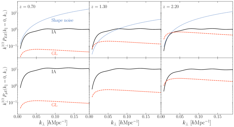
Figure 12: Impact of lensing effects on the auto power spectra of E-mode ellipticity $P_{EE}$ (upper row) and cross power spectra between density and E-mode ellipticity $P_{gE}$ (lower row), at $z=0.7$ (left), $1.30$ (middle), and $2.20$ (right), which are the lowest, central and highest redshift bins of the PFS survey, respectively. To highlight the most significant lensing impact, the power spectra shown here are the results with $k_{\parallel}=0$, and the results multiplied by $k_{\perp}^{3/2}$ are plotted as function of the transverse wavenumber, $k_{\perp}$. The red-dashed lines represent the lensing contributions (i.e., $P_{EE}^{\rm(GL)}$ and $P_{\mu E}^{\rm(GL)}$ in upper and lower panels, respectively), which are computed from equations (41) and (42), adopting the top-hat survey window ($P_{EE}^{\rm(GL)}$). The redshift bin size, $\Delta z=z_{\max}-z_{\min}$, is $\Delta z=0.2$ for $z=0.7$ and $1.3$, and $\Delta z=0.4$ for $z=2.2$. The black-solid lines are the un-lensed power spectra, $P_{EE}^{\rm(I)}$ (upper) and $P_{gE}^{\rm(I)}$ (lower), originated purely from the IA and clustering. In upper panels, we also show the non-vanishing noise contribution (see equation (30)), depicted as blue-dotted lines.

Similarly, the observed density field is altered by gravitational lensing, known as the magnification effect. By denoting the observed galaxy density field as $\delta_{\rm obs}$, one can decompose it into the intrinsic density and the term due to magnification, $\delta_{\rm obs}=\delta_{g}+\delta_{\mu}$. Then the cross power spectrum between galaxy density and ellipticity fields, $P_{gE}$, is expressed as

$$P_{gE}(\bm{k};z)=P_{gE}^{\rm(I)}(\bm{k};z)+P_{\mu E}^{\rm(GL)}(\bm{k};z),$$ (40)

where the first term is the cross power spectrum between intrinsic density and ellipticity fields considered so far, and the second term represents the lens-induced cross-power spectrum. Again, there are also cross-talk terms, the galaxy density–lensing shear $P_{gE}^{\rm(GL)}$ and magnification–intrinsic ellipticity $P_{\mu E}^{\rm(I)}$ correlations. Furthermore, the lens-induced ellipticities would be correlated with the kSZ, leading to a non-zero contamination to $P_{vE}$. Since we consider the correlation functions in individual $z$-slices, these cross-talks are negligible in our analysis.

Under the Limber approximation, $P_{EE}^{\rm(GL)}$ and $P_{\mu E}^{\rm(GL)}$ are analytically expressed as an integral of the comoving distance (e.g. Matsubara, 2000; Hui et al., 2008):

$$P_{EE}^{\rm(GL)}(\bm{k};\,z)= \left(\frac{3}{2}\frac{\Omega_{\rm m}H_{0}^{2}}{c^{2}}\right)^{2}|W_{\parallel}(k_{\parallel})|^{2}$$

$$\times\int_{0}^{\infty}d\chi^{\prime}\bigl{\{}w\bigl{(}\chi^{\prime};\chi(z)\bigr{)}\bigr{\}}^{2}\Bigl{\{}\frac{\chi(z)}{\chi^{\prime}}\Bigr{\}}^{2}$$

$$\ \ \ \ \ \ \ \ \times P_{\rm lin}\left(\frac{\chi(z)}{\chi^{\prime}}k_{\perp};\,z(\chi^{\prime})\right),$$ (41)

$$P_{\mu E}^{\rm(GL)}(\bm{k};z)= 2(\alpha_{s}-1)P_{EE}^{\rm(GL)},$$ (42)

where $\alpha_{s}$ is the logarithmic slope of the cumulative galaxy luminosity function and the lensing kernel $w(\chi^{\prime};\chi)$ is given by $w(\chi^{\prime};\chi)=(\chi-\chi^{\prime})\chi^{\prime}/\{a(\chi^{\prime})\,\chi\}\,\Theta(\chi-\chi^{\prime})$ with $\Theta(x)$ being the Heaviside step function. The function $W_{\parallel}(k_{\parallel})$ is the Fourier counterpart of the survey window function along the line-of-sight direction, $W_{\parallel}(x_{\parallel})$. Equation (42) coincides with equation (15) of Ref. Hui et al. (2008), ignoring the transverse survey window function $W_{\perp}$. Since our analysis targets spectroscopic surveys with an accurate redshift determination provided for each sample, we assume a top-hat window function,

$$W_{\parallel}(x_{\parallel})=1/\sqrt{L},\ \ \ \text{if}\ \ \bar{\chi}-L/2<x_{\parallel}<\bar{\chi}+L/2,$$ (43)

and $W_{\parallel}(x_{\parallel})=0$ otherwise. Here $L$ is the radial comoving size which corresponds to the redshift bin, given by $L=\chi(z_{\max})-\chi(z_{\min})\simeq(z_{\max}-z_{\min})\,c/H(z)$ (see table 2 for the values of $z_{\max}$ and $z_{\min}$ for each redshift bin). This top-hat window leads to $|W_{\parallel}(k_{\parallel})|^{2}=(4/Lk_{\parallel}^{2})\{\sin{(k_{\parallel}L/2)}\}^{2}$ in Fourier space. This means that the lensing contribution becomes maximum at $k_{\parallel}\ll 1$, yielding $|W_{\parallel}|^{2}\sim L$.

Figure 12 shows $P_{EE}$ (upper row) and $P_{gE}$ (lower row) at $z=0.7$, $1.30$, and $2.20$, which are the lowest, central and highest redshift bins of the PFS survey, respectively. The power spectra shown here are the results with $k_{\parallel}=0$ to highlight the maximum lensing contributions, $P_{EE}^{\rm(GL)}$ (eq. 41) and $P_{\mu E}^{\rm(GL)}$ (eq. 42). As increasing $z$, the amplitude of $P_{EE}^{\rm(GL)}$ depicted as red dashed lines in the upper row, gets larger. However, apart from the shape noise, the signal coming from the IA always dominates the E-mode power spectrum. Furthermore, the amplitude of $P_{EE}^{\rm(GL)}$ is always smaller than the shape noise expected from our fiducial setup of $\sigma_{\gamma}=0.2$, depicted as blue dotted lines. On the other hand, for the power spectrum $P_{gE}$, the amplitude is controlled by the additional parameter $\alpha_{s}$ (eq. (42)), which depends on magnitude and redshift of a given galaxy sample. We adopt the typical values of $\alpha_{s}$, $\alpha_{s}=2,2.5,$ and $3$ for $z=0.7$, $1.30$, and $2.20$, respectively (e.g., Joachimi et al., 2011). Due to the extra redshift dependence on $\alpha_{s}$, the lensing contribution to $P_{\mu E}^{\rm(GL)}$ increases faster toward higher $z$ that to $P_{EE}^{\rm(GL)}$. Nevertheless, the lensing contribution is still subdominant, and we can clearly detect the BAO signal even for the case of $k_{\parallel}=0$.

Taking the lens-induced $E$-mode ellipticity and galaxy density fields to be systematic errors, we have repeated the Fisher matrix analysis, for which the lens-induced auto power spectrum of $E$-mode and cross power spectrum of magnification and $E$-mode are included in the covariance at Eq. (27). We then confirmed that the changes in the estimated errors are negligibly small. Furthermore, instead of the top-hat filter function, we have examined another filter, the Gaussian window function, given by $|W_{\parallel}(k_{\parallel})|^{2}=\sqrt{4\pi\Sigma^{2}}\,\exp(-k_{\parallel}^{2}\Sigma^{2})$ in Fourier space. If we assume $\Sigma=L/\sqrt{4\pi}$, the contribution becomes almost equivalent to the case with the top-hat window Hui et al. (2008). If we choose a wider window, e.g., $\Sigma=L$, the amplitude of the lens-induced power spectrum becomes $\sqrt{4\pi}\sim 3.5$ times larger. Even in that case, changes in the statistical error on each parameter are still negligible, $<1\%$, namely at most the last digits of the values quoted in table 5 are modulated.

Hence, we conclude that the lensing effect on the observations of the IA gives a sub-dominant contribution to $P_{EE}$ and $P_{gE}$ as long as we consider spectroscopic surveys, and it hardly changes the cosmological constraints.

VI Conclusions

In this paper, based on the Fisher matrix analysis, we have shown that combining IA and kSZ statistics with the conventional galaxy clustering statistics substantially improves the geometric and dynamical constraints on cosmology. As a representative of deep galaxy surveys for the forecast study, we considered the Subaru PFS, whose angular area perfectly overlaps with those from the HSC survey and the CMB-S4 experiment. We found that even without the galaxy clustering, observations of IA and kSZ enable us to constrain $D_{\rm A}$ and $H$, with the achievable precision down to a few percent. This demonstrated that constraining the geometric distances with kSZ and IA effects would help addressing recent systematics-related issues such as the Hubble tension.

For cosmological parameter estimations, a relative merit of adding kSZ and IA statistics to the galaxy clustering depends on cosmological models. We found that the improvement of combining kSZ and IA to clustering statistics is maximized if we simultaneously constrain the time-varying dark energy equation-of-state parameter $w(a)=w_{0}+(1-a)w_{a}$ and the growth index $\gamma$ characterizing the modification of gravity in a non-flat universe ($w_{0}w_{a}\gamma$ non-flat model). In such a model, with the CMB prior information from the Planck experiment, the PFS-like deep survey is shown to improve the constraints by $31\%$ for $\gamma$ and $>35\%$ for others except the prior-dominated constraint on $\Omega_{K}$.

To see the gain of adding IA and kSZ for a different survey setup, we have also performed the Fisher matrix analysis for the Euclid-like wide galaxy survey, whose survey area is partly overlapped by half with the CMB-S4 experiment on the sky. Due to the large volume, such a wide survey can give tighter constraints on $f$, $D_{\rm A}$ and $H$ at each redshift bin. However, when considering the cosmological models which vary the growth index parameter, a deep survey is more effective than a wide survey, and can get tighter constraints. As a result, in the $w_{0}w_{a}\gamma$ non-flat model, by combining kSZ and IA measurements with the clustering measurement, cosmological constraints from the PFS-like deep survey can be tighter than those with the conventional clustering-only measurement from the Euclid-like wide survey. Finally, we have also discussed the potential impact of the lensing effect on the observation of IA and line-of-sight structures on the kSZ statistics, the former of which can systematically change the IA auto-power spectrum, $P_{EE}$ (see equation (40)). However, even for the deep survey considered, the lens-induced ellipticity is shown to give a negligible contribution as long as we consider the three-dimensional power spectrum, and hence the cosmological parameter estimated from the IA data is hardly changed. For the kSZ statistics, even with a large correlation length of $D_{\rm LOS}\sim 40-60\,h^{-1}$ Mpc, the impact of the line-of-sight structures on the cosmological parameters is fairly small as long as we consider a joint analysis with the galaxy clustering.

Table 6: Same as table 5 but one-dimensional fractional marginalized errors on cosmological parameters, $\sigma/\theta^{\rm fid}$, when only the data up to the linear scales $k_{\max}=0.1\,h\,{\rm Mpc}^{-1}$ are used.

			Deep survey					Wide survey
			Clustering					Clustering
Model	$\sigma/\theta^{\rm fid}$		only	+kSZ	+IA	+IA+kSZ		only	+kSZ	+IA	+IA+kSZ
$w_{0},w_{a}$	$\Omega_{\rm m}$		0.163	0.142	0.138	0.128		0.117	0.111	0.106	0.105
flat	$w_{0}$		0.452	0.415	0.404	0.377		0.327	0.317	0.309	0.303
	$w_{a}$		1.162	1.047	1.021	0.952		0.857	0.833	0.813	0.795
	$H_{0}$		0.0785	0.0679	0.0657	0.0608		0.0538	0.0509	0.0484	0.0475
$w_{0},w_{a}$	$\Omega_{\rm m}$		0.185	0.163	0.158	0.145		0.128	0.124	0.117	0.115
non-flat	$w_{0}$		0.518	0.465	0.452	0.415		0.371	0.358	0.344	0.337
	$w_{a}$		1.377	1.206	1.175	1.077		0.964	0.928	0.896	0.874
	$H_{0}$		0.0912	0.0805	0.0777	0.0715		0.0626	0.0607	0.0568	0.0560
	$100\Omega_{K}$		0.394	0.382	0.375	0.368		0.233	0.233	0.227	0.226
$w_{0},w_{a},\gamma$	$\Omega_{\rm m}$		0.277	0.187	0.179	0.150		0.170	0.152	0.135	0.126
flat	$w_{0}$		0.786	0.557	0.535	0.447		0.485	0.446	0.400	0.368
	$w_{a}$		1.862	1.359	1.310	1.107		1.222	1.140	1.032	0.948
	$H_{0}$		0.1360	0.0910	0.0867	0.0721		0.0795	0.0708	0.0623	0.0580
	$\gamma$		0.499	0.375	0.370	0.326		0.349	0.323	0.300	0.259
$w_{0},w_{a},\gamma$	$\Omega_{\rm m}$		0.345	0.217	0.207	0.169		0.243	0.208	0.168	0.151
non-flat	$w_{0}$		0.986	0.633	0.605	0.492		0.718	0.616	0.507	0.447
	$w_{a}$		2.410	1.583	1.521	1.248		1.792	1.547	1.291	1.133
	$H_{0}$		0.1722	0.1080	0.1027	0.0838		0.1212	0.1033	0.0834	0.0747
	$100\Omega_{K}$		0.439	0.392	0.384	0.371		0.305	0.285	0.259	0.247
	$\gamma$		0.559	0.386	0.380	0.329		0.459	0.397	0.343	0.284

In this paper, focusing specifically on the measurements of geometric and dynamical distortions, we have shown that the combination of both IA and kSZ with galaxy clustering is beneficial. Note, however, that the present analysis using only the BAO and RSD information is not as powerful as that using the full shape of the the underlying matter power spectrum. Although one advantage in the present analysis is that the systematics arising from the nonlinearity is less severe and hence conservative, it would be highly desirable for more tighter cosmological constraints, in particular on the neutrino masses, to make use of the full shape information Boyle and Komatsu (2018). Indeed, the analysis with the full shape of the power spectrum has been performed in the conventional galaxy clustering analysis Okumura et al. (2008); Ivanov et al. (2020); d’Amico et al. (2020); Philcox et al. (2020); Kobayashi et al. (2022). However, the analysis with full-shape information needs a proper nonlinear modeling, and compared to the modeling of the nonlinearities for clustering statistics, less studies have been made for velocity and ellipticity statistics (e.g., Okumura et al., 2014; Blazek et al., 2019; Vlah et al., 2020). Thus, before we extend our joint analysis of density, velocity and ellipticity fields to include the full-shape spectra, we need to develop models of nonlinear power spectra for the velocity and ellipticity fields and test them with numerical simulations. Such analytical and numerical analyses will be performed in future work.

Appendix A CMB prior

In this Appendix, we describe the CMB prior information added to the Fisher matrix of the LSS probes (see figure 1). In the analysis presented in this paper, the CMB prior information is used to estimate the forecast constraints on cosmological parameters, except for the minimal cosmological model ($w_{0}$ flat model).

First of all, our primary interest is how the geometric and dynamical constraints derived from the BAO and RSD measurements can be used to test cosmological models, with the power spectra of each LSS probe characterized by Eq. (37). For this purpose, we specifically use the information determined mainly from the CMB acoustic scales. We follow Ref. Aubourg et al. (2015) and use the information on $\omega_{\rm cb}\equiv\Omega_{\rm cb}h^{2}$ and $D_{\rm M}(1090)/r_{\rm d}$, fixing the energy density of neutrinos $\omega_{\nu}$ and baryon $\omega_{\rm b}$ respectively to $\omega_{\nu}=6.42\times 10^{-4}$ and $\omega_{\rm b}=0.022284$, the former of which corresponds to the total mass of $\sum{m_{\nu}}=0.06$ [eV]. Here, the $\Omega_{\rm cb}$ is the density parameter of CDM and baryons, i.e., $\Omega_{\rm cb}=\Omega_{\rm c}+\Omega_{\rm b}$. The quantity $D_{\rm M}(z)=(1+z)D_{\rm A}(z)$ is the comoving angular diameter distance Hogg (1999), and $r_{d}$ is the sound horizon at the drag epoch, for which we use the numerically calibrated approximation:

$$r_{\rm d}\simeq\frac{55.124\exp{\left[-72.3(\omega_{\nu}+0.0006)^{2}\right]}}{\omega_{\rm cb}^{0.25351}\omega_{\rm b}^{0.12807}}~{}{\rm Mpc},$$ (44)

with $\omega_{\nu}$ and $\omega_{\rm b}$ kept fixed to the values mentioned above. Ref. Aubourg et al. (2015) found that the acoustic scale information on the data vector $\Theta_{\alpha}=(\omega_{\rm cb},D_{\rm M}(1090)/r_{\rm d})$ can be described by a Gaussian likelihood with mean and covariance (see also Ivanov et al. (2020)):

$$\mu_{\Theta}=\left(0.1386,\,94.33\right),$$ (45)

$$C_{\Theta}=\begin{pmatrix}7.452\times 10^{-6}&-3.605\times 10^{-5}\\ -3.605\times 10^{-5}&0.004264\end{pmatrix}.$$ (46)

The inverse of this error matrix is the Fisher matrix, $\bm{F}_{{\rm CMB}}=\bm{C}_{\Theta}^{-1}$, shown in the lower left of the flowchart in figure 1. It is then converted to the Fisher matrix for a given cosmological model of interest, $\bm{S}_{{\rm CMB}}$, through equation (33). We have also tried another CMB prior used in our early study Taruya and Okumura (2020), based on Seo & Eisenstein Seo and Eisenstein (2003), and confirmed that our forecast results almost remain unchanged.

Appendix B Forecast results with the conservative cutoff of $k_{\max}=0.1h{\rm Mpc}^{-1}$

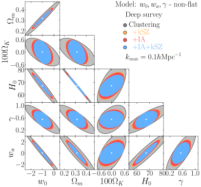
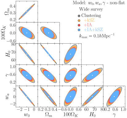
Figure 13: Cosmological constraints on the $w_{0}w_{a}\gamma$ non-flat model from the deep (Top ) and wide (Bottom) surveys. These results are similar with figure 8 but using the conservative range of data of $k_{\max}=0.1\,h\,{\rm Mpc}^{-1}$.

In sections IV and V, forecast constraints on cosmological parameters, including the geometric distances and growth of structure, were derived focusing on the upcoming deep and wide galaxy surveys, PFS and Euclid, respectively. In doing so, one important assumption was that the linear theory template for the power spectra is applicable to the weakly nonlinear scales, setting the maximum wavenumber to $k_{\rm max}=0.2\,h$ Mpc^-1 for all the three LSS probes. While our analysis is still conservative in the sense that we only use the geometric and dynamical information obtained from the BAO and RSD measurements, restricting the data to the linear scales of $k\leq 0.1\,h\,{\rm Mpc}^{-1}$ would yield a more conservative and robust forecast results, and no intricate modeling of the nonlinear systematics needs to be developed. In this appendix, repeating the Fisher matrix analysis but with $k_{\rm max}=0.1\,h$ Mpc^-1, we summarize the forecast constraints on cosmological parameters.

First we consider the deep survey. The left half of table 6 summarizes the one-dimensional marginalized errors on cosmological parameters, which are compared to results with $k_{\rm max}=0.2\,h$ Mpc^-1 listed in the left half of table 5. The results are also shown visually as the hollow bars in figure 9. The expected errors obtained from the clustering-only analysis with $k_{\rm max}=0.1\,h$ Mpc^-1 are roughly twice as large as those with $k_{\rm max}=0.2\,h$ Mpc^-1. Interestingly, however, the fractional gain of the cosmological power by adding the kSZ and/or IA measurements is more significant for the conservative analysis with $k_{\max}=0.1\,h\,{\rm Mpc}^{-1}$. For instance, in the most general model considered in this paper, namely the $w_{0}w_{a}\gamma$ non-flat model (see table 4), the improvements by $48\%$ and $41\%$, relative to the clustering-only analysis are respectively achieved for the constraints on $w_{a}$ and $\gamma$. These are compared to the relative improvements by $35\%$ and $31\%$ in the cases with $k_{\max}=0.2\,h\,{\rm Mpc}^{-1}$.

Let us then compare the forecast results for the deep survey with those for the wide galaxy survey. As seen in the right side of table 6 (see also the hollow bars in figure 9), the constraining power of the clustering-only analysis from the wide survey is $25-40\%$ stronger than that from the deep survey. This is more or less the same as the case with the aggressive cutoff of $k_{\max}=0.2\,h\,{\rm Mpc}^{-1}$. However, one notable point is that the benefit of combining the IA and kSZ measurements is more significant for the deep survey than that for the wide survey. In particular, in the $w_{0}w_{a}\gamma$ non-flat model, combining either IA or kSZ with clustering in the deep survey can beat the constraining power of the wide survey. For illustration, in figure 13, the expected two-dimensional error contours on the cosmological parameters are shown in the $w_{0}w_{a}\gamma$ non-flat model. This figure is similar with figure 8, but here we adopt the conservative cut, $k_{\max}=0.1\,h\,{\rm Mpc}^{-1}$, instead of $0.2\,h\,{\rm Mpc}^{-1}$. Clearly, the relative impact of combining IA and kSZ is rather large for the deep survey, manifesting tighter constraints not only on the growth index but also on other parameters including the curvature parameter.

References

- Peebles and Yu (1970) P. J. E. Peebles and J. T. Yu, Astrophys. J. 162, 815 (1970).
- Sunyaev and Zeldovich (1970) R. A. Sunyaev and Y. B. Zeldovich, Ap&SS 7, 3 (1970).
- Eisenstein and Hu (1998) D. J. Eisenstein and W. Hu, Astrophys. J. 496, 605 (1998), eprint arXiv:astro-ph/9709112.
- Peebles (1980) P. J. E. Peebles, The large-scale structure of the universe (Princeton, N.J., Princeton Univ. Press, 1980).
- Kaiser (1987) N. Kaiser, Mon. Not. Roy. Astron. Soc. 227, 1 (1987).
- Hamilton (1998) A. J. S. Hamilton, Linear Redshift Distortions: a Review (1998), vol. 231 of Astrophysics and Space Science Library, p. 185.
- Peacock et al. (2001) J. A. Peacock, S. Cole, P. Norberg, C. M. Baugh, J. Bland-Hawthorn, T. Bridges, R. D. Cannon, M. Colless, C. Collins, W. Couch, et al., Nature (London) 410, 169 (2001), eprint arXiv:astro-ph/0103143.
- Tegmark et al. (2004) M. Tegmark, M. A. Strauss, M. R. Blanton, K. Abazajian, S. Dodelson, H. Sandvik, X. Wang, D. H. Weinberg, I. Zehavi, N. A. Bahcall, et al., Phys. Rev. D 69, 103501 (2004), eprint arXiv:astro-ph/0310723.
- Eisenstein et al. (2005) D. J. Eisenstein, I. Zehavi, D. W. Hogg, R. Scoccimarro, M. R. Blanton, R. C. Nichol, R. Scranton, H. Seo, M. Tegmark, Z. Zheng, et al., Astrophys. J. 633, 560 (2005), eprint arXiv:astro-ph/0501171.
- Okumura et al. (2008) T. Okumura, T. Matsubara, D. J. Eisenstein, I. Kayo, C. Hikage, A. S. Szalay, and D. P. Schneider, Astrophys. J. 676, 889-898 (2008), eprint 0711.3640.
- Guzzo et al. (2008) L. Guzzo, M. Pierleoni, B. Meneux, E. Branchini, O. Le Fèvre, C. Marinoni, B. Garilli, J. Blaizot, G. De Lucia, A. Pollo, et al., Nature (London) 451, 541 (2008), eprint 0802.1944.
- Weinberg et al. (2013) D. H. Weinberg, M. J. Mortonson, D. J. Eisenstein, C. Hirata, A. G. Riess, and E. Rozo, Phys. Rept. 530, 87 (2013), eprint 1201.2434.
- Aubourg et al. (2015) É. Aubourg, S. Bailey, J. E. Bautista, F. Beutler, V. Bhardwaj, D. Bizyaev, M. Blanton, M. Blomqvist, A. S. Bolton, J. Bovy, et al., Phys. Rev. D 92, 123516 (2015), eprint 1411.1074.
- Okumura et al. (2016) T. Okumura, C. Hikage, T. Totani, M. Tonegawa, H. Okada, K. Glazebrook, C. Blake, P. G. Ferreira, S. More, A. Taruya, et al., Publ. Astron. Soc. Japan 68, 38 (2016), eprint 1511.08083.
- Alam et al. (2017) S. Alam, M. Ata, S. Bailey, F. Beutler, D. Bizyaev, J. A. Blazek, A. S. Bolton, J. R. Brownstein, A. Burden, C.-H. Chuang, et al., Mon. Not. Roy. Astron. Soc. 470, 2617 (2017), eprint 1607.03155.
- Suyu et al. (2018) S. H. Suyu, T.-C. Chang, F. Courbin, and T. Okumura, Space Sci. Rev. 214, 91 (2018), eprint 1801.07262.
- Alam et al. (2021) S. Alam, M. Aubert, S. Avila, C. Balland, J. E. Bautista, M. A. Bershady, D. Bizyaev, M. R. Blanton, A. S. Bolton, J. Bovy, et al., Phys. Rev. D 103, 083533 (2021), eprint 2007.08991.
- Takada et al. (2014) M. Takada, R. S. Ellis, M. Chiba, J. E. Greene, H. Aihara, N. Arimoto, K. Bundy, J. Cohen, O. Doré, G. Graves, et al., Publ. Astron. Soc. Japan 66, R1 (2014), eprint 1206.0737.
- DESI Collaboration et al. (2016) DESI Collaboration, A. Aghamousa, J. Aguilar, S. Ahlen, S. Alam, L. E. Allen, C. Allende Prieto, J. Annis, S. Bailey, C. Balland, et al., arXiv e-prints arXiv:1611.00036 (2016), eprint 1611.00036.
- Laureijs et al. (2011) R. Laureijs, J. Amiaux, S. Arduini, J. L. Auguères, J. Brinchmann, R. Cole, M. Cropper, C. Dabin, L. Duvet, A. Ealet, et al., arXiv e-prints arXiv:1110.3193 (2011), eprint 1110.3193.
- Capak et al. (2019) P. Capak, J.-C. Cuillandre, F. Bernardeau, F. Castander, R. Bowler, C. Chang, C. Grillmair, P. Gris, T. Eifler, C. Hirata, et al., arXiv e-prints arXiv:1904.10439 (2019), eprint 1904.10439.
- Euclid Collaboration et al. (2020) Euclid Collaboration, A. Blanchard, S. Camera, C. Carbone, V. F. Cardone, S. Casas, S. Clesse, S. Ilić, M. Kilbinger, T. Kitching, et al., Astron. Astrophys. 642, A191 (2020), eprint 1910.09273.
- Spergel et al. (2013a) D. Spergel, N. Gehrels, J. Breckinridge, M. Donahue, A. Dressler, B. S. Gaudi, T. Greene, O. Guyon, C. Hirata, J. Kalirai, et al., ArXiv e-prints (2013a), eprint 1305.5422.
- Spergel et al. (2013b) D. Spergel, N. Gehrels, J. Breckinridge, M. Donahue, A. Dressler, B. S. Gaudi, T. Greene, O. Guyon, C. Hirata, J. Kalirai, et al., arXiv e-prints arXiv:1305.5425 (2013b), eprint 1305.5425.
- Eifler et al. (2021) T. Eifler, M. Simet, E. Krause, C. Hirata, H.-J. Huang, X. Fang, V. Miranda, R. Mandelbaum, C. Doux, C. Heinrich, et al., Mon. Not. Roy. Astron. Soc. (2021), eprint 2004.04702.
- Sunyaev and Zeldovich (1980) R. A. Sunyaev and I. B. Zeldovich, Mon. Not. Roy. Astron. Soc. 190, 413 (1980).
- Ostriker and Vishniac (1986) J. P. Ostriker and E. T. Vishniac, Astrophys. J. Lett. 306, L51 (1986).
- Hernández-Monteagudo et al. (2006) C. Hernández-Monteagudo, L. Verde, R. Jimenez, and D. N. Spergel, Astrophys. J. 643, 598 (2006), eprint astro-ph/0511061.
- Okumura et al. (2014) T. Okumura, U. Seljak, Z. Vlah, and V. Desjacques, J. Cosmol. Astropart. Phys. 5, 003 (2014), eprint 1312.4214.
- Mueller et al. (2015) E.-M. Mueller, F. de Bernardis, R. Bean, and M. D. Niemack, Astrophys. J. 808, 47 (2015), eprint 1408.6248.
- Sugiyama et al. (2016) N. S. Sugiyama, T. Okumura, and D. N. Spergel, J. Cosmol. Astropart. Phys. 7, 001 (2016), eprint 1509.08232.
- Sugiyama et al. (2017) N. S. Sugiyama, T. Okumura, and D. N. Spergel, J. Cosmol. Astropart. Phys. 1, 057 (2017), eprint 1606.06367.
- Zheng (2020) Y. Zheng, Astrophys. J. 904, 48 (2020), eprint 2001.08608.
- Hand et al. (2012) N. Hand, G. E. Addison, E. Aubourg, N. Battaglia, E. S. Battistelli, D. Bizyaev, J. R. Bond, H. Brewington, J. Brinkmann, B. R. Brown, et al., Physical Review Letters 109, 041101 (2012), eprint 1203.4219.
- De Bernardis et al. (2017) F. De Bernardis, S. Aiola, E. M. Vavagiakis, N. Battaglia, M. D. Niemack, J. Beall, D. T. Becker, J. R. Bond, E. Calabrese, H. Cho, et al., J. Cosmol. Astropart. Phys. 3, 008 (2017), eprint 1607.02139.
- Sugiyama et al. (2018) N. S. Sugiyama, T. Okumura, and D. N. Spergel, Mon. Not. Roy. Astron. Soc. 475, 3764 (2018), eprint 1705.07449.
- Planck Collaboration et al. (2018) Planck Collaboration, N. Aghanim, Y. Akrami, M. Ashdown, J. Aumont, C. Baccigalupi, M. Ballardini, A. J. Banday, R. B. Barreiro, N. Bartolo, et al., Astron. Astrophys. 617, A48 (2018), eprint 1707.00132.
- Li et al. (2018) Y.-C. Li, Y.-Z. Ma, M. Remazeilles, and K. Moodley, Phys. Rev. D 97, 023514 (2018), eprint 1710.10876.
- Calafut et al. (2021) V. Calafut, P. A. Gallardo, E. M. Vavagiakis, S. Amodeo, S. Aiola, J. E. Austermann, N. Battaglia, E. S. Battistelli, J. A. Beall, R. Bean, et al., Phys. Rev. D 104, 043502 (2021), eprint 2101.08374.
- Chaves-Montero et al. (2021) J. Chaves-Montero, C. Hernández-Monteagudo, R. E. Angulo, and J. D. Emberson, Mon. Not. Roy. Astron. Soc. 503, 1798 (2021), eprint 1911.10690.
- Chen et al. (2022) Z. Chen, P. Zhang, X. Yang, and Y. Zheng, Mon. Not. Roy. Astron. Soc. 510, 5916 (2022), eprint 2109.04092.
- Croft and Metzler (2000) R. A. C. Croft and C. A. Metzler, Astrophys. J. 545, 561 (2000), eprint astro-ph/0005384.
- Heavens et al. (2000) A. Heavens, A. Refregier, and C. Heymans, Mon. Not. Roy. Astron. Soc. 319, 649 (2000), eprint astro-ph/0005269.
- Lee and Pen (2000) J. Lee and U.-L. Pen, Astrophys. J. Lett. 532, L5 (2000), eprint astro-ph/9911328.
- Pen et al. (2000) U.-L. Pen, J. Lee, and U. Seljak, Astrophys. J. Lett. 543, L107 (2000), eprint astro-ph/0006118.
- Catelan et al. (2001) P. Catelan, M. Kamionkowski, and R. D. Blandford, Mon. Not. Roy. Astron. Soc. 320, L7 (2001), eprint astro-ph/0005470.
- Jing (2002) Y. P. Jing, Mon. Not. Roy. Astron. Soc. 335, L89 (2002), eprint astro-ph/0206098.
- Hirata and Seljak (2004) C. M. Hirata and U. Seljak, Phys. Rev. D 70, 063526 (2004), eprint astro-ph/0406275.
- Heymans et al. (2004) C. Heymans, M. Brown, A. Heavens, K. Meisenheimer, A. Taylor, and C. Wolf, Mon. Not. Roy. Astron. Soc. 347, 895 (2004), eprint astro-ph/0310174.
- Mandelbaum et al. (2006) R. Mandelbaum, C. M. Hirata, M. Ishak, U. Seljak, and J. Brinkmann, Mon. Not. Roy. Astron. Soc. 367, 611 (2006), eprint astro-ph/0509026.
- Hirata et al. (2007) C. M. Hirata, R. Mandelbaum, M. Ishak, U. Seljak, R. Nichol, K. A. Pimbblet, N. P. Ross, and D. Wake, Mon. Not. Roy. Astron. Soc. 381, 1197 (2007), eprint astro-ph/0701671.
- Okumura et al. (2009) T. Okumura, Y. P. Jing, and C. Li, Astrophys. J. 694, 214 (2009), eprint 0809.3790.
- Okumura and Jing (2009) T. Okumura and Y. P. Jing, Astrophys. J. Lett. 694, L83 (2009), eprint 0812.2935.
- Blazek et al. (2011) J. Blazek, M. McQuinn, and U. Seljak, J. Cosmol. Astropart. Phys. 5, 10 (2011), eprint 1101.4017.
- Singh et al. (2015) S. Singh, R. Mandelbaum, and S. More, Mon. Not. Roy. Astron. Soc. 450, 2195 (2015), eprint 1411.1755.
- Schmidt and Jeong (2012) F. Schmidt and D. Jeong, Phys. Rev. D 86, 083513 (2012), eprint 1205.1514.
- Faltenbacher et al. (2012) A. Faltenbacher, C. Li, and J. Wang, Astrophys. J. Lett. 751, L2 (2012), eprint 1112.0503.
- Chisari and Dvorkin (2013) N. E. Chisari and C. Dvorkin, J. Cosmol. Astropart. Phys. 12, 029 (2013), eprint 1308.5972.
- Chisari et al. (2016) N. E. Chisari, C. Dvorkin, F. Schmidt, and D. N. Spergel, Phys. Rev. D 94, 123507 (2016), eprint 1607.05232.
- Okumura and Taruya (2020) T. Okumura and A. Taruya, Mon. Not. Roy. Astron. Soc. 493, L124 (2020), eprint 1912.04118.
- Okumura et al. (2020) T. Okumura, A. Taruya, and T. Nishimichi, Mon. Not. Roy. Astron. Soc. 494, 694 (2020), eprint 2001.05302.
- Taruya and Okumura (2020) A. Taruya and T. Okumura, Astrophys. J. Lett. 891, L42 (2020), eprint 2001.05962.
- Masaki et al. (2020) S. Masaki, T. Nishimichi, and M. Takada, Mon. Not. Roy. Astron. Soc. 496, 483 (2020), eprint 2003.10052.
- Akitsu et al. (2021a) K. Akitsu, T. Kurita, T. Nishimichi, M. Takada, and S. Tanaka, Phys. Rev. D 103, 083508 (2021a), eprint 2007.03670.
- Akitsu et al. (2021b) K. Akitsu, Y. Li, and T. Okumura, J. Cosmol. Astropart. Phys. 2021, 041 (2021b), eprint 2011.06584.
- Tonegawa et al. (2015) M. Tonegawa, T. Totani, H. Okada, M. Akiyama, G. Dalton, K. Glazebrook, F. Iwamuro, T. Maihara, K. Ohta, I. Shimizu, et al., Publ. Astron. Soc. Japan 67, 81 (2015), eprint 1502.07900.
- Okada et al. (2016) H. Okada, T. Totani, M. Tonegawa, M. Akiyama, G. Dalton, K. Glazebrook, F. Iwamuro, K. Ohta, N. Takato, N. Tamura, et al., Publ. Astron. Soc. Japan 68, 47 (2016), eprint 1504.05592.
- Dawson et al. (2016) K. S. Dawson, J.-P. Kneib, W. J. Percival, S. Alam, F. D. Albareti, S. F. Anderson, E. Armengaud, É. Aubourg, S. Bailey, J. E. Bautista, et al., Astron. J. 151, 44 (2016), eprint 1508.04473.
- Mandelbaum et al. (2011) R. Mandelbaum, C. Blake, S. Bridle, F. B. Abdalla, S. Brough, M. Colless, W. Couch, S. Croom, T. Davis, M. J. Drinkwater, et al., Mon. Not. Roy. Astron. Soc. 410, 844 (2011), eprint 0911.5347.
- Tonegawa et al. (2018) M. Tonegawa, T. Okumura, T. Totani, G. Dalton, K. Glazebrook, and K. Yabe, Publ. Astron. Soc. Japan 70, 41 (2018), eprint 1708.02224.
- Tonegawa and Okumura (2022) M. Tonegawa and T. Okumura, Astrophys. J. Lett. 924, L3 (2022), eprint 2109.14297.
- Shi et al. (2021) J. Shi, K. Osato, T. Kurita, and M. Takada, Astrophys. J. 917, 109 (2021), eprint 2104.12329.
- Verde et al. (2019) L. Verde, T. Treu, and A. G. Riess, Nature Astronomy 3, 891 (2019), eprint 1907.10625.
- Okumura et al. (2017) T. Okumura, T. Nishimichi, K. Umetsu, and K. Osato, arXiv e-prints arXiv:1706.08860 (2017), eprint 1706.08860.
- Okumura et al. (2018) T. Okumura, T. Nishimichi, K. Umetsu, and K. Osato, Phys. Rev. D 98, 023523 (2018), eprint 1807.02669.
- Okumura et al. (2019) T. Okumura, A. Taruya, and T. Nishimichi, Phys. Rev. D 100, 103507 (2019).
- Miyazaki et al. (2012) S. Miyazaki, Y. Komiyama, H. Nakaya, Y. Kamata, Y. Doi, T. Hamana, H. Karoji, H. Furusawa, S. Kawanomoto, T. Morokuma, et al., in Ground-based and Airborne Instrumentation for Astronomy IV (2012), vol. 8446 of Proc. SPIE, p. 84460Z.
- Aihara et al. (2018) H. Aihara, N. Arimoto, R. Armstrong, S. Arnouts, N. A. Bahcall, S. Bickerton, J. Bosch, K. Bundy, P. L. Capak, J. H. H. Chan, et al., Publ. Astron. Soc. Japan 70, S4 (2018), eprint 1704.05858.
- Abazajian et al. (2016) K. N. Abazajian, P. Adshead, Z. Ahmed, S. W. Allen, D. Alonso, K. S. Arnold, C. Baccigalupi, J. G. Bartlett, N. Battaglia, B. A. Benson, et al., arXiv e-prints arXiv:1610.02743 (2016), eprint 1610.02743.
- Chevallier and Polarski (2001) M. Chevallier and D. Polarski, International Journal of Modern Physics D 10, 213 (2001), eprint gr-qc/0009008.
- Linder (2003) E. V. Linder, Phys. Rev. Lett. 90, 091301 (2003), eprint astro-ph/0208512.
- Colgáin et al. (2021) E. Ó. Colgáin, M. M. Sheikh-Jabbari, and L. Yin, arXiv e-prints arXiv:2104.01930 (2021), eprint 2104.01930.
- Kaiser (1984) N. Kaiser, Astrophys. J. Lett. 284, L9 (1984).
- Linder (2005) E. V. Linder, Phys. Rev. D 72, 043529 (2005), eprint arXiv:astro-ph/0507263.
- Matsumoto et al. (2020) J. Matsumoto, T. Okumura, and M. Sasaki, J. Cosmol. Astropart. Phys. 2020, 059 (2020), eprint 2005.09227.
- Peacock and Dodds (1994) J. A. Peacock and S. J. Dodds, Mon. Not. Roy. Astron. Soc. 267, 1020 (1994), eprint arXiv:astro-ph/9311057.
- Scoccimarro (2004) R. Scoccimarro, Phys. Rev. D 70, 083007 (2004), eprint arXiv:astro-ph/0407214.
- Taruya et al. (2010) A. Taruya, T. Nishimichi, and S. Saito, Phys. Rev. D 82, 063522 (2010), eprint 1006.0699.
- Okumura et al. (2015) T. Okumura, N. Hand, U. Seljak, Z. Vlah, and V. Desjacques, Phys. Rev. D 92, 103516 (2015), eprint 1506.05814.
- Blazek et al. (2015) J. Blazek, Z. Vlah, and U. Seljak, J. Cosmol. Astropart. Phys. 8, 015 (2015), eprint 1504.02510.
- Blazek et al. (2019) J. A. Blazek, N. MacCrann, M. A. Troxel, and X. Fang, Phys. Rev. D 100, 103506 (2019).
- Vlah et al. (2020) Z. Vlah, N. E. Chisari, and F. Schmidt, J. Cosmol. Astropart. Phys. 1, 025 (2020), eprint 1910.08085.
- Szalay et al. (1998) A. S. Szalay, T. Matsubara, and S. D. Landy, Astrophys. J. Lett. 498, L1 (1998), eprint astro-ph/9712007.
- Szapudi (2004) I. Szapudi, Astrophys. J. 614, 51 (2004), eprint astro-ph/0404477.
- Taruya et al. (2020) A. Taruya, S. Saga, M.-A. Breton, Y. Rasera, and T. Fujita, Mon. Not. Roy. Astron. Soc. 491, 4162 (2020), eprint 1908.03854.
- Castorina and White (2020) E. Castorina and M. White, Mon. Not. Roy. Astron. Soc. 499, 893 (2020), eprint 1911.08353.
- Shiraishi et al. (2020) M. Shiraishi, T. Okumura, N. S. Sugiyama, and K. Akitsu, Mon. Not. Roy. Astron. Soc. 498, L77 (2020), eprint 2005.03438.
- Shiraishi et al. (2021a) M. Shiraishi, T. Okumura, and K. Akitsu, J. Cosmol. Astropart. Phys. 2021, 039 (2021a), eprint 2009.04355.
- Shiraishi et al. (2021b) M. Shiraishi, A. Taruya, T. Okumura, and K. Akitsu, Mon. Not. Roy. Astron. Soc. 503, L6 (2021b), eprint 2012.13290.
- Hamilton (1992) A. J. S. Hamilton, Astrophys. J. Lett. 385, L5 (1992).
- Okumura and Jing (2011) T. Okumura and Y. P. Jing, Astrophys. J. 726, 5 (2011), eprint 1004.3548.
- Fisher (1995) K. B. Fisher, Astrophys. J. 448, 494 (1995), eprint arXiv:astro-ph/9412081.
- Strauss and Willick (1995) M. A. Strauss and J. A. Willick, Phys. Rept. 261, 271 (1995), eprint arXiv:astro-ph/9502079.
- Crittenden et al. (2002) R. G. Crittenden, P. Natarajan, U.-L. Pen, and T. Theuns, Astrophys. J. 568, 20 (2002), eprint astro-ph/0012336.
- Schmitz et al. (2018) D. M. Schmitz, C. M. Hirata, J. Blazek, and E. Krause, J. Cosmol. Astropart. Phys. 2018, 030 (2018), eprint 1805.02649.
- Kurita et al. (2021) T. Kurita, M. Takada, T. Nishimichi, R. Takahashi, K. Osato, and Y. Kobayashi, Mon. Not. Roy. Astron. Soc. 501, 833 (2021), eprint 2004.12579.
- Ballinger et al. (1996) W. E. Ballinger, J. A. Peacock, and A. F. Heavens, Mon. Not. Roy. Astron. Soc. 282, 877 (1996), eprint arXiv:astro-ph/9605017.
- Seo and Eisenstein (2003) H.-J. Seo and D. J. Eisenstein, Astrophys. J. 598, 720 (2003), eprint astro-ph/0307460.
- Matsubara (2004) T. Matsubara, Astrophys. J. 615, 573 (2004), eprint arXiv:astro-ph/0408349.
- van Gemeren and Chisari (2020) I. R. van Gemeren and N. E. Chisari, Phys. Rev. D 102, 123507 (2020).
- Alcock and Paczynski (1979) C. Alcock and B. Paczynski, Nature (London) 281, 358 (1979).
- Matsubara and Suto (1996) T. Matsubara and Y. Suto, Astrophys. J. Lett. 470, L1+ (1996), eprint arXiv:astro-ph/9604142.
- Blazek et al. (2014) J. Blazek, U. Seljak, Z. Vlah, and T. Okumura, J. Cosmol. Astropart. Phys. 4, 001 (2014), eprint 1311.5563.
- Vlah et al. (2012) Z. Vlah, U. Seljak, P. McDonald, T. Okumura, and T. Baldauf, J. Cosmol. Astropart. Phys. 11, 009 (2012), eprint 1207.0839.
- Bobin et al. (2014) J. Bobin, F. Sureau, J. L. Starck, A. Rassat, and P. Paykari, Astron. Astrophys. 563, A105 (2014), eprint 1401.6016.
- Albrecht et al. (2006) A. Albrecht, G. Bernstein, R. Cahn, W. L. Freedman, J. Hewitt, W. Hu, J. Huth, M. Kamionkowski, E. W. Kolb, L. Knox, et al., arXiv e-prints astro-ph/0609591 (2006), eprint astro-ph/0609591.
- Hikage et al. (2019) C. Hikage, M. Oguri, T. Hamana, S. More, R. Mandelbaum, M. Takada, F. Köhlinger, H. Miyatake, A. J. Nishizawa, H. Aihara, et al., Publ. Astron. Soc. Japan 71, 43 (2019), eprint 1809.09148.
- Euclid Collaboration et al. (2022) Euclid Collaboration, S. Ilić, N. Aghanim, C. Baccigalupi, J. R. Bermejo-Climent, G. Fabbian, L. Legrand, D. Paoletti, M. Ballardini, M. Archidiacono, et al., Astron. Astrophys. 657, A91 (2022), eprint 2106.08346.
- Planck Collaboration et al. (2016a) Planck Collaboration, P. A. R. Ade, N. Aghanim, M. Arnaud, M. Ashdown, J. Aumont, C. Baccigalupi, A. J. Banday, R. B. Barreiro, J. G. Bartlett, et al., Astron. Astrophys. 594, A13 (2016a), eprint 1502.01589.
- Lewis et al. (2000) A. Lewis, A. Challinor, and A. Lasenby, Astrophys. J. 538, 473 (2000), eprint arXiv:astro-ph/9911177.
- Percival et al. (2007) W. J. Percival, S. Cole, D. J. Eisenstein, R. C. Nichol, J. A. Peacock, A. C. Pope, and A. S. Szalay, Mon. Not. Roy. Astron. Soc. 381, 1053 (2007), eprint 0705.3323.
- Beutler et al. (2017) F. Beutler, H.-J. Seo, S. Saito, C.-H. Chuang, A. J. Cuesta, D. J. Eisenstein, H. Gil-Marín, J. N. Grieb, N. Hand, F.-S. Kitaura, et al., Mon. Not. Roy. Astron. Soc. 466, 2242 (2017), eprint 1607.03150.
- Takada and Doré (2015) M. Takada and O. Doré, Phys. Rev. D 92, 123518 (2015), eprint 1508.02469.
- Hernández-Monteagudo et al. (2015) C. Hernández-Monteagudo, Y.-Z. Ma, F. S. Kitaura, W. Wang, R. Génova-Santos, J. Macías-Pérez, and D. Herranz, Phys. Rev. Lett. 115, 191301 (2015), eprint 1504.04011.
- Aghanim et al. (1996) N. Aghanim, F. X. Desert, J. L. Puget, and R. Gispert, Astron. Astrophys. 311, 1 (1996), eprint astro-ph/9604083.
- Planck Collaboration et al. (2016b) Planck Collaboration, R. Adam, N. Aghanim, M. Ashdown, J. Aumont, C. Baccigalupi, M. Ballardini, A. J. Banday, R. B. Barreiro, N. Bartolo, et al., Astron. Astrophys. 596, A108 (2016b), eprint 1605.03507.
- Matsubara (2000) T. Matsubara, Astrophys. J. Lett. 537, L77 (2000), eprint astro-ph/0004392.
- Hui et al. (2008) L. Hui, E. Gaztañaga, and M. Loverde, Phys. Rev. D 77, 063526 (2008), eprint 0710.4191.
- Joachimi et al. (2011) B. Joachimi, R. Mandelbaum, F. B. Abdalla, and S. L. Bridle, Astron. Astrophys. 527, A26 (2011), eprint 1008.3491.
- Boyle and Komatsu (2018) A. Boyle and E. Komatsu, J. Cosmol. Astropart. Phys. 2018, 035 (2018), eprint 1712.01857.
- Ivanov et al. (2020) M. M. Ivanov, M. Simonović, and M. Zaldarriaga, J. Cosmol. Astropart. Phys. 2020, 042 (2020), eprint 1909.05277.
- d’Amico et al. (2020) G. d’Amico, J. Gleyzes, N. Kokron, K. Markovic, L. Senatore, P. Zhang, F. Beutler, and H. Gil-Marín, J. Cosmol. Astropart. Phys. 2020, 005 (2020), eprint 1909.05271.
- Philcox et al. (2020) O. H. E. Philcox, M. M. Ivanov, M. Simonović, and M. Zaldarriaga, J. Cosmol. Astropart. Phys. 2020, 032 (2020), eprint 2002.04035.
- Kobayashi et al. (2022) Y. Kobayashi, T. Nishimichi, M. Takada, and H. Miyatake, Phys. Rev. D 105, 083517 (2022), eprint 2110.06969.
- Hogg (1999) D. W. Hogg, arXiv e-prints astro-ph/9905116 (1999), eprint astro-ph/9905116.