GGCHEMPY: A pure Python-based gas-grain chemical code for efficient simulation of interstellar chemistry^∗

Abstract

In this paper, we present a new gas-grain chemical code for interstellar clouds written in pure Python (GGCHEMPY). By combining with the high-performance Python compiler Numba, GGCHEMPY is as efficient as the Fortran-based version. With the Python features, flexible computational workflows and extensions become possible. As a showcase, GGCHEMPY is applied to study the general effects of three-dimensional projection on molecular distributions using a two-core system which can be easily extended for more complex cases. By comparing the molecular distribution differences between two overlapping cores and two merging cores, we summarized the typical chemical differences such as, N2H+, HC3N, C2S, H2CO, HCN and C2H, which can be used to interpret 3-D structures in molecular clouds.

1 Introduction

The observations of molecular lines are useful tools to study the physical and chemical processes of star-forming regions such as, chemistry in the cold stage of dark clouds ($\sim 10$ K), warm-chemistry in the warm-up stage of hot molecular cores ($\sim 10-300$ K), and shock-derived and high-temperature chemistry in molecular outflows (a few 1000 K) (e.g. Herbst & van Dishoeck 2009; Bally 2016; Jørgensen et al. 2020). To understand the chemical processes, several astro-chemical codes using rate equation method have been developed for pure gas-phase reactions (e.g. McElroy et al. 2013; Wakelam 2014), gas-phase reactions and accretion/desorption processes related to dust grains (e.g Maret & Bergin 2015), full gas-grain processes with dust surface reactions (e.g. Hasegawa et al. 1992; Hasegawa & Herbst 1993b; Garrod & Herbst 2006; Garrod et al. 2008; Semenov et al. 2010; Grassi et al. 2014; Ge et al. 2016a, b, 2020a, 2020b; Ruaud et al. 2016; Holdship et al. 2017).

Generally, the astrochemical model is a single-point one (0-D) with fixed physical parameters and a chemical reaction network. It can be applied to 1-D, 2-D and 3-D cases by sampling points with corresponding physical parameters of a complex physical structure which may need multiple steps to prepare a model for a specific case. Thus, the simplicity of the use of the code becomes an important point. Another point is that the codes written in Fortran/C are dependent on the compiler and the libraries installed in the computer system, such as the ordinary differential equation (ODE) solvers: ODEPACK in Fortran or CVODE in C. For example, some Fortran codes developed with gfortran may report errors when compiled by the Intel Fortran compiler (ifort) due to some minor syntax differences. Moreover, users should pre-build their computer environments which vary among different operating systems (Linux/Windows/Mac OS). This may be not good for some astronomers because that $\sim 63\pm 4$% astronomers have not taken any computer-science courses at an undergraduate or graduate level as reported by a survey of astronomers (Bobra et al. 2020). Therefore, a simple but powerful astro-chemistry code is desired.

With increasing Python users in astronomy (see e.g. $\sim 67\pm 2$% reported by Momcheva & Tollerud 2015 and $\sim 66$% by Bobra et al. 2020), the Python programming language is likely a good choice to solve the above issues due to its flexible syntax and power package organization, which makes Python to be system-independent. In this work, we present a gas-grain chemical code written in pure Python (GGCHEMPY) to fetch the flexible features of Python and to reach comparable speed to the existing Fortran version by using Python package Numba which translates Python functions to optimized machine code at runtime using the industry-standard low level virtual machine (LLVM) compiler library. As a showcase, GGCHEMPY is applied to discuss the three-dimensional projection effects of molecular cloud cores on molecular distributions using a two-core system with typical physical conditions of Planck galactic cold clumps (PGCCs). This serves as a complementary work of Ge et al. (2020b) which discusses the molecular projection effects in a complex and specific PGCC G224.4-0.6.

This paper is organized as follows. Section 2 describes the gas-grain code GGCHEMPY. In Section 3, the GGCHEMPY code is applied to discuss a more general projection effect on molecular distributions. Finally, a summary is given in Section 4.

2 Chemical model and code

In this section, we describe the Gas-Grain CHEMistry code written in pure Python (GGCHEMPY). It was developed on basis of the gas-grain chemical processes described in literature (e.g. Hasegawa et al. 1992; Semenov et al. 2010) and the Fortran 90 version of GGCHEM that have been used for various chemical problems in interstellar clouds (e.g Ge et al. 2016a, b; Tang et al. 2019; Ge et al. 2020a, b).

2.1 Chemical model

In the model, the gas-grain chemical processes include gas-phase reactions and dust surface reactions which linked through accretion and desorption processes of neutral species (e.g. Hasegawa et al. 1992; Semenov et al. 2010). The gas-grain reaction network from Semenov et al. (2010) is updated and used in this work. Beside the thermal and cosmic-ray-induced desorption processes (Hasegawa & Herbst 1993a), the reactive desorption (Garrod et al. 2007; Minissale et al. 2016) and CO and H2 self-shielding (Lee et al. 1996) are implemented.

The GGCHEMPY code simulates the gas-grain chemical processes by solving the Ordinary Differential Equations (ODEs) of a species $i$ in gas-phase:

$$\frac{\mathrm{d}n_{i}}{\mathrm{d}t}=\sum_{l,m}k_{lm}n_{l}n_{m}-n_{i}\sum_{i\neq l}k_{l}n_{l}+k_{i}^{\mathrm{des}}n_{i}^{s}-k_{i}^{\mathrm{acc}}n_{i},$$ (1)

and the corresponding neutral species on dust surface

$$\frac{\mathrm{d}n_{i}^{s}}{\mathrm{d}t}=\sum_{l,m}k_{lm}^{s}n_{l}^{s}n_{m}^{s}-n_{i}^{s}\sum_{i\neq l}k_{l}^{s}n_{l}^{s}-k_{i}^{\mathrm{des}}n_{i}^{s}+k_{i}^{\mathrm{acc}}n_{i},$$ (2)

where $n$ is the number density of species and $k$ is the reaction rate coefficient. The superscripts ’s’, ’des’ and ’acc’ indicate surface species, desorption process and accretion process respectively. The formulas to compute reaction rate coefficient can be found in paper of Semenov et al. (2010). The Python package scipy.integrate.ode is used to do the integration using the backward-differentiation formulas (BDF) method.

2.2 Usage and benchmark of GGCHEMPY

To avoid duplication of variable name when being combined with other codes (such as radiation transferring code), GGCHEMPY is modularized into Python classes. There are seven attributes of ggchempylib.ggchempy: gas, dust, ggpars, elements, species, reactions, iswitch. Thus, physical and chemical properties can be defined separately in the classes such as gas temperature gas.T, dust temperature dust.T, species mass species.mass etc. The class ggpars is used to store common parameters, such as constants, parameters for reaction network, parameters for ODEs, controls of time steps etc. The class iswitch is used to switch on some functions, such as H2 and CO self-shielding (Lee et al. 1996) (iswitch.iSS=1) and reactive desorption from Garrod et al. (2007) (iswitch.iNTD=1) or Minissale et al. (2016) (iswitch.iNTD=2). To switch off a function, just pass ”0” to the class.

The GGCHEMPY code can be downloaded from https://github.com/JixingGE/GGCHEMPY. To install GGCEHMPY, type the following command on the terminal:
python setup.py build
python setup.py install
After installation, GGCHEMPY can be activated via a graphical user interface (GUI) or Python script. To use the GUI, just type run_GUI() after importing it from GGCHEMPY (e.g. from ggchempylib import run_GUI). Three necessary steps are needed to run a model in a python script:

• Import necessary functions, such as from ggchempylib import ggchempy

• Set parameters according to your model in the python script

• Run the code by typing ggchempy.run(modelname)

GGCHEMPY works by calling init_ggchem() to initialize reaction network according to your input parameters. Then it computes reaction rate coefficients for all reactions by calling compute_reaction_rate_coefficients(). Finally, to solve the ODEs, BDF method from scipy.integrate.ode is used to do the integration. Here, the Numba decorator @numba.jit(nopython=True) is added to the Python functions fode(y,t) and fjac(y,t) to accelerate the integration of ODEs, which need massive calculations and loops. The modeled results will be saved into "out/DC.dat" if modelname="DC" and ggchempy.ggpars.outdir="out/". The modeled results can also be directly passed to a Python dictionary (DC) for analysis/plot in the same Python script by typing e.g. DC=ggchempy.run("DC").

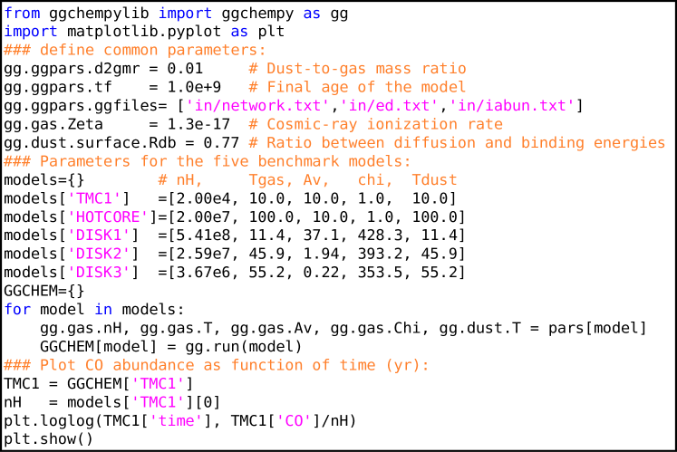
Figure 1: An exemplar python script to use GGCHEMPY to compute five benchmark chemical models and explore the results.

The benchmark of the GGCHEMPY code was successfully made with the five models from Semenov et al. (2010) using the Python script shown in Fig. 1. A laptop with Linux system and Intel i7-3612QM (4 cores, 2.1 GHz) was used. The Python version is 3.8.5. For one model, GGCHEMPY can finish within about 10 seconds which is comparable to the Fortran version, see Fig 2. The benchmark results and screenshot of GUI and the full documents can be found on the GGCHEMPY webpage.

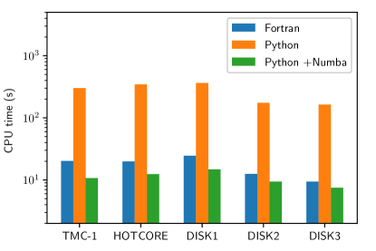
Figure 2: Comparison of CPU times used by the Fortran code (GGCHEM, blue) and GGCHEMPY (without (orange) and with Numba (green)) for the five benchmark models of TMC1, HOTCORE, DISK1, DISK2 and DISK3.

3 A showcase: three-dimensional projection effects

As a showcase in this section, GGCHEMPY is applied to combine with physical models to study general three-dimensional projection effects on molecules (TDPEs). The TDPE was proposed by Ge et al. (2020b) for a Planck galactic cold clump (PGCC) G224.4-0.6 with four cores interpreted from observations which is a special one constrained by observed molecules of N2H+, HC3N and C2S. The MHD simulation of filamentary molecular clouds made by Li & Klein 2019 could also support the TDPEs. Considering the TDPEs could commonly exist in space, we explore a more general TDPE with more molecules. In addition, the chemical differences between the overlapping cores and the merging cores are not explored yet which are important for interpreting observations and are also the goals in this section.

To study general TDPEs, typical physical conditions of PGCCs are adopted because that

• The PGCCs have typical conditions of $T_{\rm dust}\sim 7-20$ K and $N_{\rm H_{2}}\sim 10^{20}-5\times 10^{22}$ cm^-2 (e.g. Planck Collaboration et al. 2011a, b, 2016; Wu et al. 2012; Mannfors et al. 2021). They have been continuously studied via observations by many projects (e.g. Wu et al. 2012; Liu et al. 2012, 2018; Tatematsu et al. 2017; Tang et al. 2018, 2019; Yi et al. 2018; Eden et al. 2019; Dutta et al. 2020; Sahu et al. 2021; Yi et al. 2021; Wakelam et al. 2021) with notable molecular peak offsets from continuum peaks, such as N2H+, HC3N and C2S in samples of PGCCs (Tatematsu et al. 2017, 2021) and C2H in a PGCC G168.72-15.48 (Tang et al. 2019). Therefore, they are ideal sources to verify the TDPEs through observations.

• The typical physical conditions of PGCCs provide observable information for our large JCMT project SPACE in which one of the scientific goals is to verify the TDPEs through observable molecular distributions.

In the following sections, physical models are described in Section 3.1. We describe spherical core with the Plummer-like physical structure in Section 3.1.1 which is used as a basic unit to build the following two-core systems: two overlapping cores along line-of-sight in Section 3.1.2 and a face-on two merging cores in Section 3.1.3 as a comparison. Results and discussions are shown in Section 3.3 and 3.4 respectively. Considering the complexity of 3-D structures and the purpose of the showcase, we do not explore more parameter space, such as the variation of parameters to build a Plummer-like core, the viewing angle of the two merging cores etc. To facilitate the comparison with the two-overlapping-cores model, we only consider the orientation of the two-merging-cores model when both cores are in the same sky plane and we call it ”face-on”.

3.1 Physical models

3.1.1 Spherical cloud core (SCC)

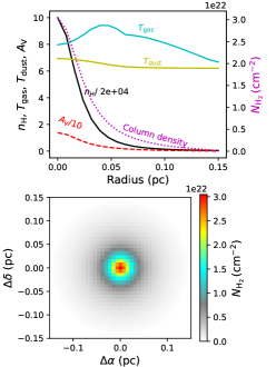
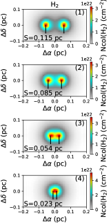
Figure 3: Left-top: radial profiles of density (cm^-3), extinction (mag), gas and dust temperatures (K). Left-bottom: H2 column density map. Right: H2 column density maps of two overlapping cores with different separations ($S$, values shown with labels and marked by vertical lines) from top to bottom for S1 to S4, which serve as continuum maps. Right panels with limited ranges of axes to show central part.

For a spherical cloud core, we use the 1-D radial density profile described by the Plummer-like function (Plummer 1911)

$$n(r)=\frac{n_{c}}{(1+(r/r_{c})^{2})^{p/2}}$$ (3)

where $n_{c}$ is the central density, $r_{c}$ is the central flat region and $p$ is the pow-law index.

We set the needed parameters by Eq.(3) according to the following physical conditions of PGCCs. For PGCCs in $\lambda$ Orionis cloud, Orion A and B, Yi et al. (2018) reported the cloud cores with [$R=0.08$ pc, $n_{\rm H}=(2.9\pm 0.4)\times 10^{5}$ cm^-3], [$R=0.11$ pc, $n_{\rm H}=(3.8\pm 0.5)\times 10^{5}$ cm^-3] and [$R=0.16$ pc, $n_{\rm H}=(15.6\pm 1.8)\times 10^{5}$ cm^-3] in which $R$ is the radius of the core. For PGCCs in the L1495 dark cloud, Tang et al. (2018) derived central densities of $n_{c}\sim 1.3\times 10^{4}-1.8\times 10^{5}$ cm^-3 with $r_{c}\sim 0.01-0.1$ and outer radius of $R\sim 0.06-1.0$ pc. Considering the above parameters derived from observations, we set $n_{c}$, $r_{c}$ and $R$ in our model to be $2\times 10^{5}$ cm^-3, 0.025 pc and $0.15$ pc respectively. The $p$ value is set to be 3.0 which is an intermediate one (e.g. $p\sim 1.5-4.3$ for the four PGCCs used in the work of Ge et al. (2020b)).

We sample 20 radial points with a resolution of $1628$ AU for the 1-D radial physical profile. Thus, a cube with $39\times 39\times 39$ points is built for a spherical cloud core by interpolating on the 1-D physical profile. The 2-D column density map $N_{\rm H_{2}}(x,y)$ is obtained by integrating along the line of the sight ($z$). In Fig. 3, the left-top and left-bottom panels show the radial physical profiles and the H2 column density map respectively, showing that the values at the center and edge are about $3.06\times 10^{22}$ and $2.95\times 10^{20}$ cm^-2 respectively.

The visual extinction is estimated using the relation to H2 column density $N_{\rm H_{2}}(r)$ (Güver & Özel 2009) via

$$A_{\rm V}=N_{\rm H_{2}}(r)/2.21\times 10^{21},$$ (4)

Here we neglect the mutual shielding effects between the two cores. The extinctions vary from $\sim 13.80$ mag (center) to $\sim 0.13$ mag (edge). The radial gas and dust temperatures are estimated using the formulas from Goldsmith (2001), considering cooling and heating processes of molecules and the effects of coupling between the gas and the grains. The extinction and temperature profiles are shown in the left-top panel of Fig. 3.

3.1.2 Two overlapping cloud cores (TOCC)

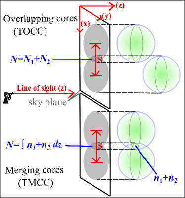
Figure 4: Sketches of the two overlapping cloud core model (TOCC, upper part) and the two face-on merging cloud core model (TMCC, lower part). $n$ and $N$ are number density and column density respectively.

To study the TDPEs, we adopt a simple model with two same spherical cores with an adjustable separation ($S$) on the sky plane (see the upper part of Fig. 4). The H2 column density map of the two overlapping cloud cores (hereafter TOCC) is reached by summing the column density maps of the two cores with an assumption of optically thin and an adjustable separation ($S$): $N_{\rm H_{2}}=\int_{-R}^{+R}n_{1}(x,y,z)dz+\int_{-R}^{+R}n_{2}(x,y,z)dz$, where $z$ is the line-of-sight direction. Four $S$ values are adopted and shown with labels together with the H2 column density maps in the right panels of Fig. 3. The modeled peak values of H2 column density is about $3-5\times 10^{22}$ cm^-2 which is consistent with the lower limits ($2.5\times 10^{22}$ cm^-2) derived from a sample of PGCCs (Yi et al. 2018).

3.1.3 Two merging cloud cores (TMCC)

We also build a model with two merging cloud cores at the same sky-plane to compare the chemical differences with the TOCC model (see the lower part of Fig. 4). Since the gravitational stability of such a system is not the concern of this work, the physical models will stay unchanged during the chemical model evolution. At the merged part, the gas densities are first summed before running chemical models which results in a H2 column density map with $N_{\rm H_{2}}=\int_{-R}^{+R}(n_{1}(x,y,z)+n_{2}(x,y,z))dz$. For estimating the visual extinction, we simply calculate six values from six directions at each grid point and adopt the minimum one but timing a factor of 2.0 to match the one derived from Eq.(4)) along the line of sight.

3.2 Chemical structure

To simulate the chemical structures of the above physical models, GGCHEMPY is called as a Python module. For an SCC model, chemical models with 20 radial points can be finished within CPU time of about $200=20\times 10$ seconds. For the TOCC model, two same chemical structures of the SCC model can be used with an adjustable separation under the optically thin assumption. However, for the TMCC model, a large number of single-point chemical models are needed to build a 3-D chemical structure because that the densities should be first summed at the merged parts. For example, about 14 days is needed for a 3-D grid of $39\times 78\times 39$ with 10 seconds for one model. Even considering the symmetry, the CPU time can only be reduced from 14 days to  1.7 days (14/8). In addition, we also need to change the merged parts according to the varying separation which needs more time. To reduce the computation time, we build a mode grid with varied density, extinction and temperature which results in about 700 models and needs about 3 hours to run (see details in Appendix A). Once the models on the grids are finished, only $\sim 15$ seconds are needed to load them. Thus, the modeled abundances at any given parameters can be obtained by interpolating on the grid. The interpolated values are compared with the true model with explicit parameters in Fig. 15 in Appendix A. In this way, the computation time is highly reduced. For the TMCC models, we use a fixed temperature of 10 K for both gas and dust grains. Comparing to the models with varied gas and dust temperatures, we find that the temperature effects on molecular abundances are very small, see discussions in Section 3.4.1.

3.3 Results

Typical molecules are discussed such as, N2H+, HCO+, HCN, HC3N, H2CO, C2H, C2S and SO, in which some of them are tracers of the SPACE project. To simulate molecular column density maps, we turn on the switch of GGCHEMPY to include the reactive desorption (hereafter RD) proposed by Minissale et al. (2016) which is important for the cloud core models. The column density maps of molecules are obtained by combining the chemical models on the TMCC and TOCC physical model grids at given ages. Fig. 5-10 show the modeled column density maps of selected species. In these figures, the grayscale shows the H2 column density map. The cyan and red contours show the maps from TMCC and TOCC models respectively with levels of $(0.3\,,0.6\,,0.9)\times N_{\rm max}$ where $N_{\rm max}$ is the maximum column density of a species. Comparing the modeled peak column densities at age of $5\times 10^{5}$ yr with the observed ones of N2H+ ($\sim 10^{12}-10^{13}$), HCN ($\sim 10^{12}-10^{14}$), H2CO ($\sim 10^{13}-10^{14}$) and C2H ($\sim 10^{14}-10^{15}$) in PGCCs within $\lambda$ Orionis, Orion A and B clouds (Yi et al. 2021), we found that good agreements are reached within typically one order of magnitude. The panel ID in form of (Sn,age) is to indicate the modeled result with a given separation from the four sets (n=1,2,3,4) defined in Section 3.1.2 and a given age.

3.3.1 Chemical differences between TMCC and TOCC models

For N2H+ in Fig. 5, the TOCC model and the TMCC model have similar distributions except for the one in panel (S3,5e4). This is because that the depletion effects of N2H+ is very small due to its parent species N2 having high gas-phase abundance (Womack et al. 1992). The N2H+ peak in the TOCC model (red) in panel of (S3,5e4) is due to superposition of the flat abundance distributions of N2H+ in the sky area between the two cores. This occurs when the size of the N2H+ central flat region is comparable to the separation between the two cores.

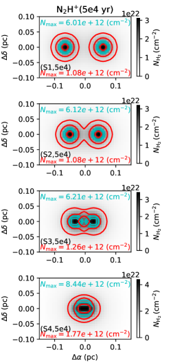
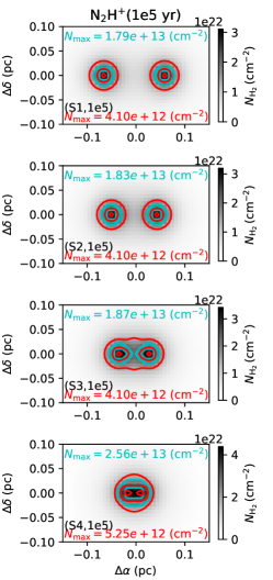
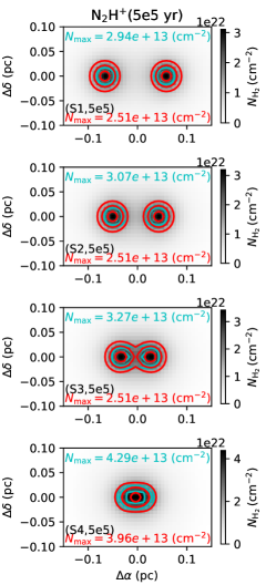
Figure 5: Modeled N2H+ column density maps from TMCC model (cyan contours) and TOCC model (red contours) overlapping on H2 column density map (gray scale), with varied ages of $5\times 10^{4}$, $10^{5}$, $5\times 10^{5}$ yrs for left, middle and right panels respectively. The contours with levels of $(0.3\,,0.6\,,0.9)\times N_{\rm max}$ where $N_{\rm max}$ is the maximum column density of N2H+ shown as texts.

For HC3N in Fig. 6 and C2S in Fig. 7, two big differences between TMCC(red) and TOCC (red) models are found at later ages of $10^{5}$ and $5\times 10^{5}$ yrs when the depletion effects take effect. (1) At age of $10^{5}$ yr, the depletion effects start to occur resulting in a small ring structure around each core in the TOCC model. Thus, there are two peaks (red in panels of (S4,1e5)) with linked axis perpendicular to the x-axis; (2) At a later age of $5\times 10^{5}$ yr, the peak offset from the two H2 peaks in the TOCC model (red in panel of (S3,5e5)) is also due to the projection effects. For the TMCC model, depletion effects are larger at the merged parts due to the higher densities, which results in no molecular peak here. Similar behaviors are also found for H2CO, HCN and C2H shown in Fig. 8, 9 and 10 respectively. These results are also in accord with the modeling of PGCC in paper of Ge et al. (2020a), though the physical models are different.

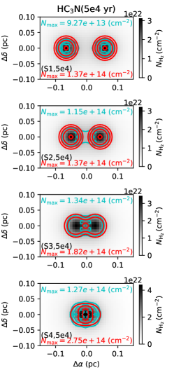
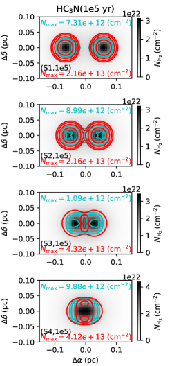
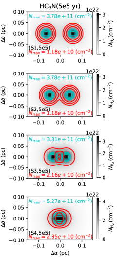
Figure 6: Same as Fig. 5, but for HC3N.

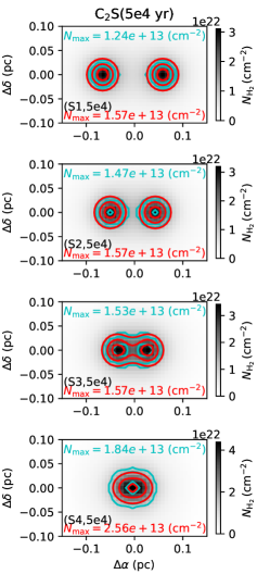
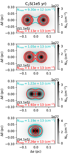
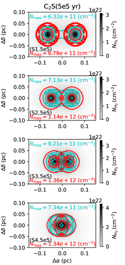
Figure 7: Same as Fig. 5, but for C2S.

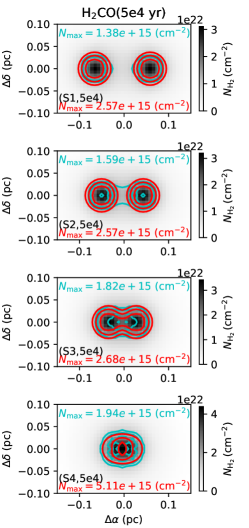
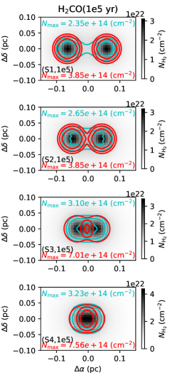
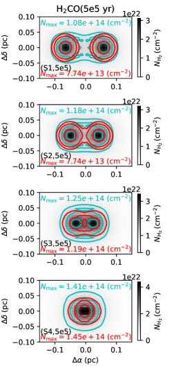
Figure 8: Same as Fig. 5, but for H2CO.

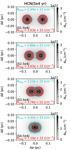
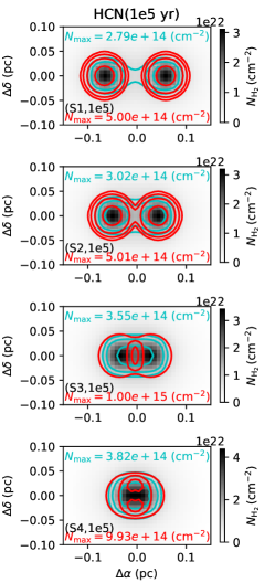
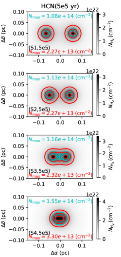
Figure 9: Same as Fig. 5, but for HCN.

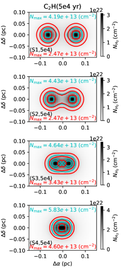
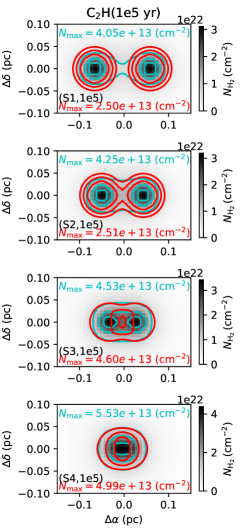
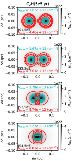
Figure 10: Same as Fig. 5, but for C2H.

Molecular peak offsets can also be observed at the middle of the two cores in the TMCC model at early ages, such as that (cyan) shown in panel (S3,5e4) of Fig. 6, 8 and 9 for HC3N, H2CO and HCN respectively. The molecular peaks are due to that, at the peak position, the depletion does not occur at so early ages. But for the continuum peaks (gray) with higher density, the depletion starts to take effect.

Finally, we summarize typical molecular differences between the TOCC and TMCC models in the left-most part of Fig. 11 which shows four patterns marked by names of P1, P2, P3, and P4. In the right parts of Fig. 11, to clearly show the differences as function of separation and chemical age, the panel’s ID in Figs. 5-10 (e.g. (S1,1e5)) are listed for the above species accordingly. By checking Fig. 11, we find that, for N2H+, the patterns P1 and P3 are observed at early ages of 5e4 and 1e5 yrs. However for HC3N, C2S, H2CO, HCN and C2H, patterns P1, P2 and P4 are observed at later ages of 1e5 and 5e5 yrs. For all the species except for N2H+, the patterns are usually observed for the two cores with separations of S3 (0.054 pc) and S4 (0.023 pc). The above trends indicate that the peaks observed in the TOCC models strongly depend on the ring size of molecules, e.g the radial peak of C2S at $\sim 0.05$ pc at a later age of about $1\sim 5\times 10^{5}$ yr (see e.g. Fig. 14). This also means that true physical structures from observations are the key points to reproduce observed molecular distributions by applying the projection effects.

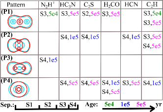
Figure 11: Summary of four typical patterns (P1/2/3/4) of molecular distribution differences between the two overlapping cloud core model (red) and the two merging cloud core model (cyan). The separations (S1=0.115, S2=0.085, S3=0.054 and S4=0.023 pc) and chemical ages ($t=$5e4, 1e5 and 5e5 yr) of corresponding species that shown in Fig. 5-10 are summarized in the right part.

In summary, the molecular peak offsets from the H2 map peaks can be observed at many evolutionary stages (ages) due to the projection effects of the two cores in 3-D space which show different distributions as that of two merging cloud cores. Therefore, the molecular peak offsets from continuum peaks can be used to verify the TDPEs and then to explore 3-D structures. Applied to PGCCs, the peak offsets can be up to $\sim 0.05$ pc corresponding to $\sim 24.5^{\prime\prime}$ with the distance of PGCCs in Orion A and B (420 pc) which are observable.

3.3.2 Application: a map with randomly distributed multiple cloud cores

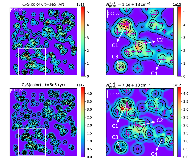
Figure 12: C2S column density map (color) with projection effects of random distributions of 200 cores at ages of $10^{5}$ (upper panels) and $5\times 10^{5}$ yrs (lower panels). Right panels show enlarged regions in the white boxes in the left panels. The black contours show the N2H+ map with levels of [0.1, 0.3, 0.5, 0.7, 0.9]$\times N_{\rm peak}^{\rm N_{2}H^{+}}$. The values of $N_{\rm peak}^{\rm N_{2}H^{+}}$ are labeled in the titles of the right panels. The purple plus signs indicate the core centers before the projection process. A white scale bar is plotted in the upper-left corner of the panels. Four cores (C1/2/3/4) are marked for discussions in the text.

To show the projection effects of molecules with multiple cloud cores, we present a synth map with 200 random cores in a $1.5\times 1.5$ pc² region. The spherical cloud core described in Section 3.1.1 is used to build the 200 cores in the region. Then the projection process described in Section 3.1.2 is used to make the synth map using random positions of the 200 cores in the region.

We choose C2S as our main example because that (1) at an early age of $10^{5}$ yr, the depletion effect is small at each core center which can be used as a non-depletion example; (2) At a later age of $5\times 10^{5}$ yr, the depletion is strong resulting in a ring structure of C2S which is a typical case. For comparison, a continuum map is indicated using N2H+ map from the same model, which is a well known dense core tracer that can be used to roughly indicate the continuum peaks. In addition, N2H+ is roughly optically thin which allows the projection process to make the map. We also take HC3N as another example to briefly compare with C2S and previous observations below.

Fig. 12 shows the synth map with C2S as color and N2H+ as black contours. As have mentioned above, two ages of $10^{5}$ and $5\times 10^{5}$ yrs are shown in the upper and lower panels respectively. The left and right panels show the whole map and an enlarged region to show typical distributions, respectively. From the right-upper panel, we see that C2S and N2H+ have similar peak positions (e.g. at positions of cores C1 to C4) at the early age of $10^{5}$ yr at which the depletion of C2S is not strong in each core. However from the right-lower panel at the later age of $10^{5}$ yr, C2S peak offsets from the N2H+ peaks are obvious (e.g. at positions of cores C1 to C4, and the cores between C1 and C2, between C2 and C4, and between C2 and C3) which are due to the strong depletion of C2S in each core. The clumpy structures of C2S are also notable which are usually observed in real interstellar clouds such as, observed C2S in a sample of PGCCs (Tatematsu et al. 2017).

The HC3N map is shown with color scale in Fig. 13 which shows that HC3N has similar peak positions as that of N2H+ (contours) at the later age ($5\times 10^{5}$ yr, lower panels) due to its weaker depletion effect than that of C2S. Many other molecules also show similar distributions as that of C2S and/or HC3N such as H2CO, HCN, C2H and SO.

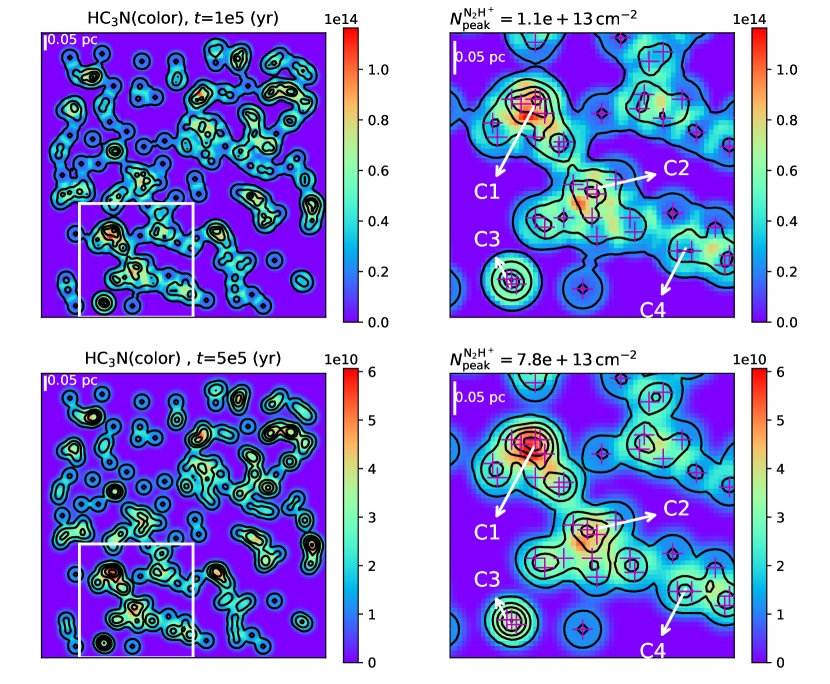
Figure 13: Same as Fig. 12 but with color scale for HC3N.

Typically, the modeled map show similar distributions to observed maps of N2H+, HC3N and C2S in some observations:

• At the early age, our modeled C2S and N2H+ have similar peak positions (upper panels in Fig. 12) as that in TUKH021 in Orion A cloud shown in Fig.3 of Tatematsu et al. (2010) (hereafter T10), showing similar peak positions of the two molecules. At the later age, our modeled C2S show peak offsets from N2H+ peaks (lower panels Fig. 12) as that observed in TUKH003 in Fig.2 and TUKH122 in Fig.7 of T10, showing C2S peak offsets from N2H+ peaks. Similar distributions were also observed in samples of PGCCs (e.g. Tatematsu et al. 2017, 2021).

• At the two ages, our modeled C2S and HC3N (see color scales in Fig. 12 and Fig. 13) have similar distributions (see distributions toward core C1) to that observed in dark cloud L1147 by Suzuki et al. (2014) (hereafter S14), see their Fig.2 and 3, showing that HC3N has similar peak position as the dust continuum map while C2S not. The age range in our model is also consistent with the proposed age of $\sim 10^{5}$ yr by the model of S14.

With the synth map of 200 cloud cores, we have shown that the projection effects could produce similar molecular distributions as that of observations. Thus, it has great potential to explain real observations and to explore 3-D structures through molecular distributions. We also note that the synth map is very rough since we assumed that all the 200 cores are independent objects in 3-D space which allows the projection process. In real interstellar clouds, complex 3-D structures could exist which means that merging cores and overlapping cores could co-exist in the same region. Another point is that there are multiple cores in a dense region (see purple plus signs in Fig. 12 towards to the C1 core) which means that complex 3-D structure in the line-of-sight exits but maybe missed by observations. Finally, we used the same physical structure for all cores which maybe not be reasonable in real space. All of these need more high-resolution observations of more molecular lines to constrain the models and to explore the true 3-D structures.

3.4 Discussions

3.4.1 Temperature effects

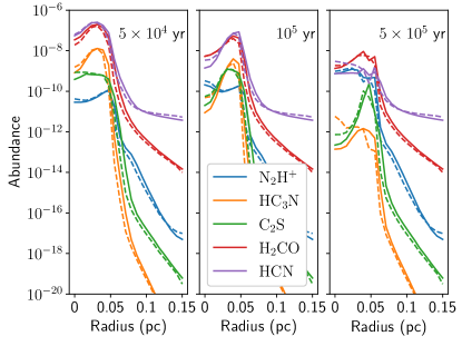
Figure 14: Temperature effects on the radial abundance profiles of N2H+, HC3N, C2S, H2CO and HCN, at ages of $5\times 10^{4}$ (left), $10^{5}$ (middle) and $5\times 10^{5}$ yrs (right). The solid lines are from the models with varied gas and dust temperatures described in Section 3.1.1. The dashed lines are from the models with a fixed temperature of 10 K for both gas and dust.

In this subsection, we demonstrate that the above 3D projection effects are not affected by the use of different gas and dust temperatures in TOCC and TMCC models. We recall that radial profiles of dust and gas temperatures computed in Sect. 3.1.1 are used in the TOCC models while homogeneous gas and dust temperatures (10 K) are adopted for the TMCC models. To examine the potential impact of the different temperatures on our discussions, we set up a new TOCC model by replacing the radial gas and dust temperature profiles with the same homogeneous temperature of 10 K as in the TMCC models. Fig. 14 shows the radial abundances of N2H+ HC3N, C2S, H2CO and HCN, at ages of $5\times 10^{4}$ (left), $10^{5}$ (middle) and $5\times 10^{5}$ yrs (right). The solid and dashed lines are from models with varied temperature and fixed temperature respectively.

From Fig. 14, we see that most species at all the selected ages have very small differences between solid and dashed lines which means that the temperatures used in our TOCC and TMCC models do not change our above conclusions. However, for HC3N at a later age of $5\times 10^{5}$ yr (yellow in the right panel), a higher temperature of 10 K (dashed) enhances its abundance due to that it is linked to N2 which has low desorption temperature from dust grains and high gas-phase abundance (Womack et al. 1992). The N2H+ and HCN are also tightly linked to N2, but they have bigger gas-phase abundances than that of HC3N. This is the reason why only HC3N have big enhancements at 10 K. Since the temperature variations ($10-15$ K) do not affect the modeled radial peaks of molecules (e.g. N2H+, HC3N and C2S) in chemical models as shown in Fig. 10 of Ge et al. (2020b), we do not test these temperatures in this work. In summary, the temperatures used in our TOCC and TMCC models do not affect our conclusions on the molecular distribution differences.

3.4.2 Isotopes

The tracers of our SPACE project also include isotopes (e.g. C^18O and DNC), which is not included in the current models. However, we can expect similar distributions of isotopes as that of their main forms because that D-bearing and ^13C-bearing species have similar evolutionary trends (depletion effects) (see e.g. modeled NH3 and NH2D in Fig.2, and HNC and HN^13C in Fig.7 of Roueff et al. (2015)) and distributions (see e.g. observed CO and ^13CO in a sample of PGCCs by Wu et al. (2012), and C3H2 and ^13CH2 in starless core L1544 by Spezzano et al. (2017)) to their main isotopes, similar three-dimensional projection effects are also expected.

3.4.3 Application to real clouds

In this work, the models are taken as showcases to show that GGCHEMPY code is efficient for building 1-D, 2-D and 3-D simulations taking one typical set of physical parameters of PGCCs. Although we have drawn some useful conclusions from our models, we should keep in mind that complex 3-D structures exist in the real space which may result in complex projection effects (see e.g. projection effects from MHD simulations of Li & Klein (2019)). Application of it to more complicated cloud models is one thing. Another point is that real clouds are clumpy and irregular. This can distort the simplistic pictures given in this paper. Thus, modeling and observations at higher spatial resolutions will be important to unambiguously recognize the 3D projection effects and to constrain the 3D structures of real clouds.

4 Summary

In this paper, we present the new pure Python-based gas-grain chemical code (GGCHEMPY). By using the Numba package, besides the flexible Python syntax, GGCHEMPY reaches a comparable speed to the Fortran-based versions and can be used for chemical simulations efficiently.

As a showcase, 1-D, 2-D and 3-D physical and chemical models are shown upon typical conditions of Planck galactic cold clumps to study chemical differences of different physical structures. By comparing the modeled molecular peaks with the H2 peaks in the overlapping two-core cloud model, we find that the molecular peak offsets from the H2 peaks can be used to trace the projection effects due to the depletion effects and projection effects and to indicate the evolutionary stages. Compared to the models with a merged two-core cloud model, the molecular distribution differences can be used to distinguish the two 3D cloud structures which have great potential to explain real observations. These simulated peak offsets caused by the three-dimensional projection effects support our scientific goal of the SPACE project towards a sample of Planck Galactic cloud clumps. Future works including isotopes and dust size distribution will be done to interpret observations.

Appendix A Interpolation on model grid

To reduce computation time, we introduce an interpolating method on a model grid. We build the single-point chemical model grid with varied density, extinction and temperature which results in about 700 models and needs about 3 hours to run (see Table 1). For each density, the extinction values vary within reasonable values. Thus the temperature values are set to reasonable values according to the correlation between extinction and dust temperature (e.g. $T(A_{\rm V}=0.1)\sim 17$ K and $T(A_{\rm V}=20)\sim 7$ K, see Hocuk et al. 2017) with considerations of wide possible uncertainties. We assume the same temperature for gas and dust grains in the models.

Therefore, the modeled abundance can be quickly estimated by interpolating on the grid with any given set of density, extinction and temperature. Two strategies are used to do the interpolation of a species at a given age: (1) When the given density is in the grid shown in the first column of Table 1, the species abundance is interpolated on the 2-D extinction-temperature map at the given age; (2) If the given density is not in the density grid, two nearest densities are selected. Thus two abundances values are obtained using the same process used in (1). Finally, the species abundance is the average one of the two abundances. Fig. 15 shows the good agreements between the interpolated values (cross) and the true models (line) which show very small differences.

Table 1: Model grid

$n_{\rm H}$ (cm-3)	$A_{\rm V}$(mag)	$T$ (K)
$10^{2}$	0.1, 0.5, 1, 1.5, 2	18, 17, 16, 15, 14, 13, 12, 11, 10
$5\times 10^{2}$	0.1, 0.5, 1, 1.5, 2	18, 17, 16, 15, 14, 13, 12, 11, 10
$10^{3}$	0.1, 0.5, 1, 2, 3, 4, 5	16, 15, 14, 13, 12, 11, 10
$5\times 10^{3}$	0.1, 0.5, 1, 2, 3, 4, 5	16, 15, 14, 13, 12, 11, 10
$10^{4}$	1, 2, 3, 4, 5, 6, 7, 8, 9, 10, 11, 12, 13, 14, 15, 16	14, 13, 12, 11, 10, 9, 8
$5\times 10^{4}$	1, 2, 3, 4, 5, 6, 7, 8, 9, 10, 11, 12, 13, 14, 15, 16	14, 13, 12, 11, 10, 9, 8
$10^{5}$	5, 6, 7, 8, 9, 10, 11, 12, 13, 14, 15, 16, 17, 18	12, 11, 10, 9, 8, 7, 6
$5\times 10^{5}$	5, 6, 7, 8, 9, 10, 11, 12, 13, 14, 15, 16, 17, 18	12, 11, 10, 9, 8, 7, 6
$10^{6}$	5, 6, 7, 8, 9, 10, 11, 12, 13, 14, 15, 16, 17, 18	12, 11, 10, 9, 8, 7, 6

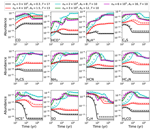
Figure 15: Comparison between interpolated values on grids (cross) and the values from true models (line) with five sets of parameters shown in the top legends.

References

- Bally (2016) Bally, J. 2016, ARA&A, 54, 491
- Bobra et al. (2020) Bobra, M. G., Mumford, S. J., Hewett, R. J., et al. 2020, Sol. Phys., 295, 57
- Dutta et al. (2020) Dutta, S., Lee, C.-F., Liu, T., et al. 2020, ApJS, 251, 20
- Eden et al. (2019) Eden, D. J., Liu, T., Kim, K. T., et al. 2019, MNRAS, 485, 2895
- Garrod & Herbst (2006) Garrod, R. T., & Herbst, E. 2006, A&A, 457, 927
- Garrod et al. (2007) Garrod, R. T., Wakelam, V., & Herbst, E. 2007, A&A, 467, 1103
- Garrod et al. (2008) Garrod, R. T., Weaver, S. L. W., & Herbst, E. 2008, ApJ, 682, 283
- Ge et al. (2020a) Ge, J., Mardones, D., Inostroza, N., & Peng, Y. 2020a, MNRAS, 497, 3306
- Ge et al. (2016a) Ge, J. X., He, J. H., & Li, A. 2016a, MNRAS, 460, L50
- Ge et al. (2016b) Ge, J. X., He, J. H., & Yan, H. R. 2016b, MNRAS, 455, 3570
- Ge et al. (2020b) Ge, J. X., Mardones, D., He, J. H., et al. 2020b, ApJ, 891, 36
- Goldsmith (2001) Goldsmith, P. F. 2001, Astrophys. J., 557, 736
- Grassi et al. (2014) Grassi, T., Bovino, S., Schleicher, D. R. G., et al. 2014, MNRAS, 439, 2386
- Güver & Özel (2009) Güver, T., & Özel, F. 2009, MNRAS, 400, 2050
- Hasegawa & Herbst (1993a) Hasegawa, T. I., & Herbst, E. 1993a, MNRAS, 261, 83
- Hasegawa & Herbst (1993b) Hasegawa, T. I., & Herbst, E. 1993b, MNRAS, 263, 589
- Hasegawa et al. (1992) Hasegawa, T. I., Herbst, E., & Leung, C. M. 1992, ApJS, 82, 167
- Herbst & van Dishoeck (2009) Herbst, E., & van Dishoeck, E. F. 2009, ARA&A, 47, 427
- Hocuk et al. (2017) Hocuk, S., Szucs, L., Caselli, P., et al. 2017, Astron. Astrophys., 604, 58
- Holdship et al. (2017) Holdship, J., Viti, S., Jiménez-Serra, I., Makrymallis, A., & Priestley, F. 2017, AJ, 154, 38
- Jørgensen et al. (2020) Jørgensen, J. K., Belloche, A., & Garrod, R. T. 2020, ARA&A, 58, 727
- Lee et al. (1996) Lee, H. H., Herbst, E., Pineau des Forets, G., Roueff, E., & Le Bourlot, J. 1996, A&A, 311, 690
- Li & Klein (2019) Li, P. S., & Klein, R. I. 2019, MNRAS, 485, 4509
- Liu et al. (2012) Liu, T., Wu, Y., & Zhang, H. 2012, ApJS, 202, 4
- Liu et al. (2018) Liu, T., Kim, K.-T., Juvela, M., et al. 2018, ApJS, 234, 28
- Mannfors et al. (2021) Mannfors, E., Juvela, M., Bronfman, L., et al. 2021, arXiv e-prints, arXiv:2106.10114
- Maret & Bergin (2015) Maret, S., & Bergin, E. A. 2015, Astrochem: Abundances of chemical species in the interstellar medium
- McElroy et al. (2013) McElroy, D., Walsh, C., Markwick, A. J., et al. 2013, A&A, 550, A36
- Minissale et al. (2016) Minissale, M., Dulieu, F., Cazaux, S., & Hocuk, S. 2016, A&A, 585, A24
- Momcheva & Tollerud (2015) Momcheva, I., & Tollerud, E. 2015, arXiv e-prints, arXiv:1507.03989
- Planck Collaboration et al. (2011a) Planck Collaboration, Ade, P. A. R., Aghanim, N., et al. 2011a, A&A, 536, A22
- Planck Collaboration et al. (2011b) Planck Collaboration, Ade, P. A. R., Aghanim, N., et al. 2011b, A&A, 536, A23
- Planck Collaboration et al. (2016) Planck Collaboration, Ade, P. A. R., Aghanim, N., et al. 2016, A&A, 594, A28
- Plummer (1911) Plummer, H. C. 1911, MNRAS, 71, 460
- Roueff et al. (2015) Roueff, E., Loison, J. C., & Hickson, K. M. 2015, A&A, 576, A99
- Ruaud et al. (2016) Ruaud, M., Wakelam, V., & Hersant, F. 2016, MNRAS, 459, 3756
- Sahu et al. (2021) Sahu, D., Liu, S.-Y., Liu, T., et al. 2021, ApJ, 907, L15
- Semenov et al. (2010) Semenov, D., Hersant, F., Wakelam, V., et al. 2010, A&A, 522, A42
- Spezzano et al. (2017) Spezzano, S., Caselli, P., Bizzocchi, L., Giuliano, B. M., & Lattanzi, V. 2017, A&A, 606, A82
- Suzuki et al. (2014) Suzuki, T., Ohishi, M., & Hirota, T. 2014, Astrophys. J., 788, 108
- Tang et al. (2018) Tang, M., Liu, T., Qin, S. L., et al. 2018, arXiv, 856, 141
- Tang et al. (2019) Tang, M., Ge, J. X., Qin, S.-L., et al. 2019, ApJ, 887, 243
- Tatematsu et al. (2010) Tatematsu, K., Hirota, T., Kandori, R., & Umemoto, T. 2010, Publ. Astron. Soc. Japan, 62, 1473
- Tatematsu et al. (2017) Tatematsu, K., Liu, T., Ohashi, S., et al. 2017, ApJS, 228, 12
- Tatematsu et al. (2021) Tatematsu, K., Kim, G., Liu, T., et al. 2021, arXiv e-prints, arXiv:2106.04052
- Wakelam (2014) Wakelam, V. 2014, Nahoon: Time-dependent gas-phase chemical model
- Wakelam et al. (2021) Wakelam, V., Gratier, P., Ruaud, M., et al. 2021, A&A, 647, A172
- Womack et al. (1992) Womack, M., Ziurys, L. M., & Wyckoff, S. 1992, Astrophys. J., 393, 188
- Wu et al. (2012) Wu, Y., Liu, T., Meng, F., et al. 2012, ApJ, 756, 76
- Yi et al. (2021) Yi, H.-W., Lee, J.-E., Kim, K.-T., et al. 2021, ApJS, 254, 14
- Yi et al. (2018) Yi, H.-W., Lee, J.-E., Liu, T., et al. 2018, ApJS, 236, 51