revtex4-2Repair the float
Quantum Chaos and Universal Trotterisation Behaviours in Digital Quantum Simulations
Abstract
Digital quantum simulation (DQS) is one of the most promising paths for achieving first useful real-world applications for industry-scale quantum processors. Yet even assuming continued rapid progress in device engineering and successful development of fault-tolerant quantum processors, extensive algorithmic resource optimisation will long remain crucial to exploit their full computational power. Currently, among leading DQS algorithms, Trotterisation provides state-of-the-art resource scaling. And recent theoretical observations of a distinct breakdown threshold in empirical performance for Trotterised Ising models suggest that even better performance than expected may be possible prior to the threshold.
Here, to start exploring this possibility, we study multiple paradigmatic DQS models with experimentally realisable Trotterisations, and provide strong evidence for universality of a range of Trotterisation performance behaviours, including not only the threshold, but also new features in the pre-threshold regime that is most important for practical applications. In each model, we observe a distinct Trotterisation threshold shared across widely varying performance signatures; we further show that an onset of quantum chaotic dynamics causes the performance breakdown and is directly induced by digitisation errors. In the important pre-threshold regime, we are able to identify new distinct regimes displaying qualitatively different quasiperiodic performance behaviours, and show analytic behaviour for properly defined operational Trotter errors. Our results rely crucially on diverse new analytical tools, and provide a previously missing unified picture of Trotterisation behaviour across local observables, the global quantum state, and the full Trotterised unitary. This work provides new insights and tools for addressing important questions about the algorithm performance and underlying theoretical principles of sufficiently complex Trotterisation-based DQS, that will help in extracting maximum simulation power from future quantum processors.
1 Introduction
Quantum simulation offers exciting opportunities for quantum processors to tackle the “in-silico” modelling of complex quantum systems that is often intractable for even the most advanced classical computing technology [1]. In analogue quantum simulation, a controllable, specialised surrogate is engineered to directly emulate the dynamical properties of the full target system, with rapid scaling of noisy intermediate-scale quantum (NISQ) processors being achieved for models in condensed-matter physics [2, 3, 4, 5, 6] and lattice gauge theories [7, 8, 9]. In digital quantum simulation (DQS) [10], complex target dynamics is instead constructed in discrete steps from a sequence of simpler interaction primitives (gates) on a more generic processor. This versatile approach offers universal programmability that is not limited to models which can be mapped in toto onto systems realisable naturally in a laboratory environment, and has been used to simulate highly varied target models across quantum chemistry [11, 12, 13, 14], ultrastrong coupling [15, 16, 17], condensed-matter [18, 19, 20, 21, 22] and high-energy [23] physics.
A digital gate-based approach offers compatibility with future universal quantum computers [10] and the capacity for error correction to overcome the noise and decoherence limiting the power of NISQ devices [24]. Yet it also introduces digitisation errors intrinsic to the algorithm which are reduced through finer and more sophisticated discretisation [10, 25, 26, 27, 28, 29, 30, 31, 32, 33, 34, 35]. Typically, this increases the required experimental resources (in terms of gates, qubits or runtime) and the exposure to noise, thus creating a trade-off between sufficient discretisation (algorithmic errors) and acceptable hardware noise (gates, decoherence, etc). In medium-term NISQ applications, DQS resource requirements can be somewhat reduced by combining the discretisation that increases versatility and accessible complexity, with analogue toolbox primitives to maximally exploit architecture-specific efficiencies [18, 19, 20, 22, 15, 16, 17]. Ultimately, however, for both NISQ devices and even fully error-corrected quantum processors, simulation power will for a long time be limited by such resource constraints. It is therefore an essential open problem to improve our fundamental understanding of digitisation error and how much can be tolerated for a given application, and if possible, how to compensate or correct it.
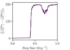
A key ongoing goal for DQS research is to better understand the computational performance of DQS algorithms with a view to bringing tasks of interest within reach of practical quantum processors and generally maximising their achievable computational power. In deriving worst-case error bounds from the full Trotterised unitary, many early works [10, 36, 37, 38] predicted very poor scaling of Trotter errors with simulation time and system size, giving rise to very pessimistic assessments about the practical feasibility of DQS. Over time, it has been shown that these bounds can be improved by means of more sophisticated implementations of Trotterised gate sequences [39, 37, 40, 41, 42], even to the extent that Trotterisation can match or outperform other state-of-the-art digitisation algorithms [34, 35]. Yet exact numerical calculations for specific DQS models have shown that even the best rigorous bounds are often orders of magnitude "loose" compared with empirical performance [39, 43, 44, 34, 42, 35]. Indeed, recent studies of Trotterised Ising models [45, 46] have even observed a rather sharp empirical performance threshold (Fig. 1) that was not previously predicted by rigorous, worst-case bounds, which they link to a transition between regions of localised dynamics and quantum chaotic dynamics. In addition, their observation of controllable, perturbative errors for some asymptotically time-averaged observables in the small-step regime, suggests that Trotterised simulations using large (but pre-threshold) step sizes may provide access to near-ideal (error-free) performance results through extrapolation. These works highlight the need for a much better understanding of operationally relevant Trotterisation performance (not just worst case) in the context of concrete DQS models.
In this work, we carry out a broad and systematic study of empirical Trotterisation performance across diverse, paradigmatic models and a wide range of Trotter step sizes. Synthesising the results from numerous different and complementary performance signatures, our work provides new insights into Trotterisation performance, including in the “good simulation” regime that is of key importance for DQS applications, as well as demonstrating marked universality for a range of performance behaviours, including both the threshold itself and new features in the pre- and post-threshold regimes. Crucial to these new insights are both our systematic approach and our introduction of diverse new analytical tools, including new approaches for exploring detailed system dynamics, well-defined error metrics for observables, and quantitatively rigorous global signatures of quantum chaos based on random matrix theory (RMT). These tools enable us to study the same behaviours in situations that cannot be straightforwardly generalised to a well-defined classical limit, which is critical for DQS, since interesting use cases most commonly correspond to models which cannot be simulated classically [47, 48, 49, 50]. In addition to providing a deeper understanding of Trotterisation performance, the advances in this work motivate a range of new and interesting directions.
The paper is organized as follows. In Sec. 1.1, we provide, up front, an overview of our key results and contributions. In Sec. 2, we provide key background information about Trotterisation, its Floquet interpretation, and quantum chaos (with more detailed background on quantum chaos in Appendix A). Sec. 3 describes the physical models and their experimentally accessible Trotterisations. After presenting our detailed findings from individual analytical approaches in Sec. 4, we discuss in Sec. 5 the broader, overarching conclusions we can establish by combining our results, along with new and open questions raised by our work, and the outlook for addressing them. Due to the significant extent of analysis and results reported in Sec. 4 and the relevant appendices, Sec. 5 is written to be rather self-contained, so that the reader may skip to this section and understand how our results support the broad conclusions of our work, and delve into the detailed results as required.
1.1 Overview of Results
1.1.1 Universality
In this paper, we analyse varied, detailed aspects of Trotterisation performance for a wide range of concrete models to further explore the potential for improvements offered over generic bounds [39, 43, 44, 34, 42, 35, 45, 46]. By studying experimentally realisable Trotterisations of the Heisenberg [19, 20], Rabi-Dicke [15, 16, 17], and all-to-all Ising (A2A-Ising) [46] models, we draw conclusions that apply to a wide range of contexts, such as influence of different symmetries, simulation with non-qubit components, systems with infinite-dimensional Hilbert spaces, and systems without clear classical limits. We identify and provide strong evidence for the universality of a range of performance behaviours across system contexts, especially in the important pre-threshold regime of Trotterised DQS. For example, we demonstrate that quantum chaotic dynamics emerges even in a highly structured and symmetric Heisenberg spin model that has no well-defined classical limit. We show these behaviours are reflected consistently across diverse physical signatures and system properties, and use new tools to provide a consistent understanding across all signatures. Importantly, our systematic and detailed analysis also allows us to identify new pre- and post-threshold behaviours in Trotterisation performance.
1.1.2 Analysis techniques
The systematic analysis underpinning our results was crucially enabled by the introduction of a range of new analytical tools and techniques covering both evolution dynamics and static properties of the Trotterised step unitary. As well as filling in important gaps in results, these new approaches have opened up important new questions about DQS performance, while also providing valuable new tools for addressing them. Similarly to techniques introduced to characterise quantum processors in terms of targeted signatures such as entanglement witnesses, gate and channel fidelities, much of our focus in this work is on more easily operationally measurable signatures (such as local observables). These offer better experimental accessibility and scaleability over inefficient full-system characterisation, such as state or process tomography. Such focussed approaches are particularly relevant and well suited to DQS, where the usual aim is to analyse and estimate the values or evolution of physical quantities of interest, such as ground-state energies [12, 13, 14] or a phase transition order parameter [3, 5, 6].
Full system dynamics
Studying the full system dynamics is arguably the most natural way to study DQS in experiments [18, 20, 21, 16], but can require some ingenuity to extract useful understanding from a large volume of data. Our analysis shows that detailed dynamics can already directly reveal valuable insights and information both qualitative and quantitative in nature. For example, we show that a shared threshold can be observed across all signatures studied, including the simulation fidelity, which was previously thought not to exhibit a persistent threshold based on analysis from time averages only [46]. Studying the full dynamics, together with the corresponding Fourier spectra (only accessible from the full dynamics), also shows very clearly how quasiperiodic dynamics (with distinct spectral frequencies) before the threshold, is destroyed after the threshold (with spectra becoming effectively flat). Arguably even more important are the insights we are able to obtain about Trotterisation performance in the pre-threshold regime, discussed further below.
Operational error metrics
Finding the best ways to extract useful quantitative information about simulation errors in a condensed, digestible form from detailed system dynamics nevertheless remains an important challenge, especially for experiments where errors from unitaries [10, 36, 35] or the outcomes of phase estimation [11, 12, 38] are often either inaccessible or resource intensive. Previous work on the Trotterisation threshold therefore focussed primarily on time-averaged and asymptotic-time errors and local observables [45, 46]. Yet practical DQS requires understanding performance over finite times, and we show here that the time-averaged quantities do not distinguish the targeted information from discrete sampling errors, which arise under time averaging even for ideal system dynamics. We therefore introduce new point-to-point time-averaging metrics which properly disentangle Trotter errors from sampling effects. These new metrics allow us to show that both local observables and simulation fidelities exhibit analytic, perturbative behaviours in the all-important pre-threshold regime, and demonstrate they depend in a sensible way on system size and simulation time, contradicting conclusions suggested by long-time error metrics [45].
Conclusive agreement with RMT signatures
Given the suggested link [45, 46] between Trotterisation performance breakdown and the emergence of quantum chaos, a key aim of our research was to identify a system- and model-agnostic way to objectively diagnose agreement with quantum chaotic dynamics directly from a Trotterised unitary. In particular, we were interested in obtaining definitive answers for cases at modest system sizes (to be relevant for currently accessible experiments) and cases without meaningful classical limit (of particular relevance for quantum computing and DQS, where quantum advantage demands systems cannot be represented classically [47, 51]). Unfortunately, while common dynamical signatures of quantum chaos (like fidelity decay and out-of-time-order correlators) can be intuitive, they provide only indicative but inconclusive evidence for quantum chaos [52, 53, 54]. The results can also be highly initial-state dependent, making it unwieldy to use dynamical signatures to extract information about the global dynamics. References [45, 46] also study signatures based on the underpinning RMT description of quantum chaotic dynamics in terms of random unitary evolution, using characteristic derived RMT quantities such as average level (eigenphase) spacings. In this work, we introduce a new, quantitatively rigorous diagnostic signature for quantum chaos in unitary quantum evolution, based on RMT predictions of the eigenvector statistics for a random unitary operator [55, 56] (see also Appendix A.3). Our approach defines a reduced chi-squared goodness-of-fit test statistic, , to provide a statistically objective, “black-box” assessment of how well a given unitary operator agrees with the predictions for a particular RMT universality class. This has two important benefits: it diagnoses agreement at the full statistical distribution level, and therefore avoids ambiguities that arise from studying individual statistical moments such as mean values, and benefits from the existence of closed-form analytical predictions for RMT eigenvector statistics that do not exist for RMT eigenvalue statistics. This works for individual unitary operators, arbitrary dimensions, all system and model types, and irrespective of whether a meaningful classical limit exists. Our work lays the groundwork for broader use of this technique in diverse areas such as quantum complexity in quantum computing [47, 48, 49, 50, 57], Floquet physics and many-body physics [58, 59, 60, 61].
1.1.3 Threshold to quantum chaos
The main results from the two previous works on Ising model DQS by some of the authors can be broadly categorised as follows: Reference [45] demonstrated the existence of a previously unobserved performance threshold marking a transition between localised and delocalised dynamical regimes, along with indirect dynamical signatures of quantum chaotic behaviour in the delocalised regime. Then, by considering the special case of the A2A-Ising model, Ref. [46] showed that the Trotterised model and its threshold could be understood in terms of quantum chaos in the kicked top based on its well-studied classical limit, but this connection does not generalise to other models. In this work, using the results from our new tools across varied model types, we demonstrate a deeper and more conclusive generic connection between DQS performance thresholds and the onset of quantum chaos than previous works [45, 46], including for modest system sizes and for systems with no clear classical limit. Specifically, we see both quasiperiodic (non-quantum chaotic) behaviour (from full dynamics and Fourier spectra) and clear analytic errors (from properly defined operational metrics) before the threshold, and provide a new quantitative and objective demonstration of quantum chaos in Trotterised unitaries after the threshold. Thus, we see that the onset of quantum chaos at the threshold marks a fundamental transition from a regime of “meaningful” approximate simulation of some target unitary, to one categorised by uncorrectable and uncontrollable errors, in other words a total breakdown in simulation performance. And by deliberately studying regular (non-quantum chaotic) target models, we demonstrate that this onset is caused directly by Trotterisation errors.
1.1.4 Unified picture of Trotterisation behaviours
Combining the results from our systematic analysis, across diverse system and model types and signatures, has also allowed us to develop a new, unified understanding of Trotterisation performance and behaviour, across local and global signatures, and state-specific versus process level measures. Previous analysis suggested that errors in local observables were surprisingly robust against both system size and simulation time before the threshold, in stark contrast to both the full unitary dynamics and the simulation fidelity of the global quantum state, with a fragile simulation fidelity threshold being swamped by pre-threshold errors and no longer even observable at larger system sizes [45, 46]. In this work, however, we not only demonstrate clear signatures of the shared threshold for local observables, the global quantum state, and the full Trotterised unitary, but also show that observables and state fidelities both exhibit clear analytic behaviours and mutually consistent size- and time-dependence. We also show that seemingly inconsistent simulation fidelity behaviours can be explained in terms of clear new pre-threshold performance regimes that we can identify from the full dynamics. Also, the coherent periodic behaviour of the simulation fidelity before the threshold provides suggestive opportunities for studying possible perturbative mitigation of Trotterisation errors at the state level (not only for the observables). These results provide significant new insight about markedly universal Trotterisation performance behaviours especially in the pre-threshold regime that is most important for DQS.
Stable regions
The full system dynamics also reveals a series of stable (non-quantum chaotic) regions beyond the threshold, where the quantum chaotic (non-quasiperiodic) dynamics are to some degree interrupted. In the Heisenberg DQS model, we account for these regions analytically as a form of digital aliasing. In the A2A-Ising DQS model, we connect the appearance of these islands phenomenologically with the re-emergence of stable islands in the collective spin phase space, by exploiting the equivalence of the Trotterised model [46] to a quantum kicked top. Based on these observations, we term them “stable regions”. In general, these revivals in stability occur for step sizes close to some periodicity in the Trotterised dynamics, usually in one of the Trotter step’s constituent gates, and “freezes out” that component of the contributing dynamics. They can be more or less pronounced depending on the choice of initial state and the prominence of underlying symmetries in the system Hilbert space and Trotterisation recipe. The stable regions are typically also much less prominent in the simulation fidelities, because the digitisation-induced regular dynamics does not necessarily in any way match the underlying, non-digitised target dynamics. We leave a more detailed analysis of these digitisation-induced stable regions as a goal for future research.
2 Background
This section summarises the relevant concepts from Trotterisation and quantum chaos, introducing the notations and definitions that are used in the rest of the manuscript. In all the equations here, we take .
2.1 Trotter Errors
In Trotterisation, the target model Hamiltonian is decomposed into a sum of experimentally accessible Hamiltonians . Then, the desired time evolution is approximated by a sequence of discrete time evolution operators for corresponding Hamiltonians , according to [10]
| (1) |
where we define the (Trotter) step size as the ratio of total simulated time and number of (Trotter) steps . Defining the unitary operators and for a single and Trotter steps, respectively, the approximation errors can be defined using a Taylor series expansion [10]
| (2) |
where subsumes the higher-order corrections. Eq. (1) is a generic example of first-order Trotterisation, but in general the unitary operations in a Trotter step are determined also by a Trotterisation order. The approximation errors for (i.e. ) for fixed , and the rate of convergence to continuum depends on the order of the Trotterisation [26, 27, 28, 29]. Trotter-Suzuki approximations (at any order) become exact when all the summands commute, but this is commonly not satisfied. Additionally, in practice, is always finite, so we target a maximum error (for fixed simulated time ) and try to determine the Trotter step size (for a particular Trotterisation order) required to achieve the desired accuracy.
The usual assumption in Eq. (2) is that the first-order error term dominates (and consequently bounds) the errors, but this intuition does not always hold [35]. A more concrete bound on the error can be obtained by using a tail bound of the Taylor expansion [36]. This worst-case bound scales, at best, linearly with simulation time [36], and can be expressed in terms of the required number of steps that ensures an error for a (th)-order Trotterisation [36, 42]:
| (3) |
where the is the spectral-norm, is the number of summands, and is any positive integer.
Though Trotterisations provide convenient implementations of direct Hamiltonian decompositions, the scaling of the gate estimate in Eq. (3) with time, system size, and other parameters draws a pessimistic picture for the product formulas. Consequently, alternative, so-called post-Trotter DQS algorithms [30, 31, 32, 33], with different overheads such as requirements for auxiliary qubits, have been developed to overcome the apparent inefficiency of Trotterisation. But while the generic estimates of gate complexities, such as Eq. (3), provide sufficient conditions for the desired accuracy [36], empirical analyses of Trotterisation algorithms show that such rigorous estimates are often loose, and the desired accuracy is typically already achieved for orders of magnitude fewer steps than the estimates [39, 37, 38, 43, 44, 42, 35]. Additionally, recent rigorous theory results [35], providing improved bounds on Trotter errors, showed that Trotterisation can match or even outperform the state-of-the-art post-Trotter algorithms, suggesting that Trotterisation may even be the optimal algorithm. Also note that the performance of Trotterisation algorithms might be improved even further by exploiting commutations between summands [39, 34] and/or by randomised ordering of unitary evolutions in each Trotter step [40, 41, 42].
Since we focus on Trotterisation algorithms in this paper, we may, unless otherwise specified, use DQS to refer specifically to Trotterisation.
2.2 Trotterisation Sequences as Floquet Systems
In addition to gate complexities, it is equally important to know the nature of the errors and the minimum (maximum ) at which the approximation is still valid. For example, before the complete breakdown point of the approximation due to coarse digitisation [45, 46], it may still be possible to correct the errors. Alternatively, it may also be possible to predict the (i.e. ) value for a particular choice of observable from a smaller number of steps.
An alternative approach to Trotter error analyses [45, 46] is to interpret the Trotterised evolution as the stroboscopic dynamics under a Floquet Hamiltonian ,
| (4) |
The digitisation error in the effective Floquet Hamiltonian is then quantified by the Floquet-Magnus (FM) expansion,
| (5) |
where subsumes any higher-order corrections. The Floquet-Magnus expansion has a finite radius of convergence , beyond which the approximation breaks down. Theoretically, this represents the largest step size for which Trotterisation will realise a meaningful approximate simulation (that is, where the Trotterisation’s effective Hamiltonian can still be understood in terms of the target Hamiltonian plus some controllable error perturbation that increases with Trotter step size). Taking the Floquet-Magnus expansion as a special case of a more general Magnus expansion for a periodically time-dependent Hamiltonian, a rigorous sufficient condition of convergence can be derived that suggests that the radius of convergence should scale in inverse proportion to system size [62, 63, 64]. If this lower bound on were tight, its scaling with inverse system size would suggest that realising large system sizes should be very challenging.
As discussed in the introduction, two recent numerical works studying DQS of the Ising model by some of the authors [45, 46] identified a performance threshold in Trotter step size (a threshold ) separating a region of controllable errors from a quantum chaotic regime. A work investigating where the Floquet-Magnus expansion diverges saw a similar threshold in Floquet heating [65]. Moreover, by interpreting the Trotterised evolution as a periodically time-dependent quantum system, Refs [45, 46] showed that pre-threshold Trotter errors for the Ising DQS in dynamical quantities such as expectation values, rather than errors in the full time evolution operator (), agree with the perturbative corrections predicted by the Floquet-Magnus expansion [45]. Some localised instability regions were observed more recently in [66] only for specific mean-field, kicked multispin models, but no such instabilities have emerged in either Refs [45, 46] or in the much wider range of models considered in this paper. The findings of Refs [45, 46] therefore open up interesting potential avenues for achieving better practical results with accessible performance, even for NISQ-era DQS. For example, perturbative treatments could enable extrapolation of ideal dynamics (i.e. ) from the simulations with finite Trotter step sizes . This would effectively circumvent the impact of Trotter errors by allowing accurate simulation results to be calculated from simulations run over a range of comparatively large Trotter step sizes, and would simultaneously also help minimise the impact of errors extrinsic to the algorithm, such as decoherence and imperfect gates. In addition to our broader results about new Trotterisation performance behaviours, our work also extends the scope of these findings and helps elevate the observations (that were mainly limited to Ising models) from Refs [45, 46] to the status of a universal DQS principle.
2.3 Quantum Chaos
In contrast to classical chaos, where infinitesimal differences in initial states diverge exponentially in time, the unitarity of dynamics in quantum mechanics ensures that the overlap between two arbitrary initial states stays the same for all times ,
where is the fidelity between the states and . But while the notion of quantum chaos does not naïvely follow popular concepts of classical chaos, similar intuitive signatures can still be found in quantum dynamics. For example, the perturbation fidelity between two states evolved from the same initial state under two slightly different unitaries and a perturbed , , decays exponentially for quantum chaotic systems [67]. Unfortunately, although this interpretation is intuitive, this fidelity decay signature is reliable only for appropriate perturbations [52].
There are many other dynamical signatures of quantum chaos [53], and all of them (including the reliability of a perturbation for fidelity decay [52]) derive from certain features governing the eigenvectors of either a unitary evolution operator, or equivalently its corresponding Hamiltonian. For quantum chaotic systems, the eigenvectors show certain random matrix properties, namely that the distribution of their components in another basis follow specific distributions from random matrix theory (RMT) [55, 56]. This type of analysis, known as eigenvector statistics, underlies the study of quantum chaos that will be described in this work. A more detailed overview of quantum chaos, its relation with RMT, and technical subtleties in calculating the signatures of quantum chaos are provided in Appendix A.
Throughout this paper, we use quasiperiodic, stable, or regular interchangeably to mean non-quantum chaotic.
3 Physical Models and Their Trotterisations
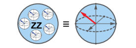

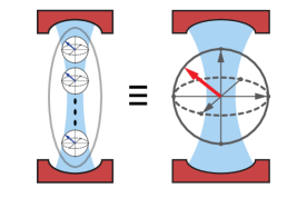
To obtain a more comprehensive understanding of the effects of Trotterisation on DQS performance (including not only the threshold observed in Refs [45, 46], but also, e.g., pre-threshold behaviours), we consider a set of paradigmatic model systems, which share the feature that their Trotterised dynamics could be realisable experimentally in the near future: the (i) Ising (in all-to-all interactions limit), (ii) Heisenberg, and (iii) Rabi-Dicke models. In this section, we provide descriptions of the model Hamiltonians and their experimentally realisable Trotter-Suzuki decompositions. Since our goal is to investigate Trotterisation performance behaviours, we do not provide either an extensive or a complete summary (or references) of these models. They are extensively studied fundamental quantum models describing magnetism (Ising and Heisenberg [68]) and light-matter interactions (Rabi-Dicke [69, 70, 71, 72, 73]), and they and their various generalisations and modifications offer rich physical phenomena and practical applications, such as quantum phase transitions (in Ising [74, 75, 76], Heisenberg [77], and Dicke and Rabi models [70, 78]), and even mappings to NP problems [79].
3.1 Spin Models
The general spin-spin interaction Hamiltonian [68]
| (7) |
defines the Heisenberg interaction for , Ising interaction for & , and the exchange (or XY-) interaction for & , where are the Pauli spin operators with . The structure of the coefficients defines further variations in each case [68]. Here, we consider all-to-all ( ) and one-dimensional nearest-neighbour () interactions for the Ising and Heisenberg models, respectively.
3.1.1 The Ising Model
Trotterisation thresholds in Ising-model DQS have been considered for various regimes of power-law interactions in Refs [45, 46]. Here, we revisit the all-to-all (A2A) case, and reveal new insight into Trotterisation performance and the threshold behaviours. In this limit, the DQS model maps to the quantum kicked top [46], and reduces to a collective spin system with total spin , as depicted in Fig. 2 (a), facilitating the study of Trotterisation performance behaviours up to relatively large system sizes. Here, we describe the corresponding quantum kicked-top model and the effective target Hamiltonian, and refer to Ref. [46] for further details of the model. Specifically, the corresponding Trotter-Suzuki decomposition is given by the kicked-top Floquet operator
| (8) |
where is the effective target-model Hamiltonian. The individual summand Hamiltonians are
| (9) |
for , with standard angular momentum operators of a spin system, corresponding to the (maximal) collective spin of spin-1/2 systems in an A2A-Ising system [46]. The quantum kicked-top models have already been implemented in various platforms, including in a single Caesium atom with [80], the collective spin of an ensemble of three superconducting qubits [22] corresponding to , and others (including novel proposals [81]) discussed in Ref. [46].
For ease of comparison and consistency, we show our results for the same simulation parameters as in Ref. [46], that is (with time measured in units of for all models), , , and , and the initial state is , where is the spin coherent state. The qualitative behaviour of our results does not depend on the precise values of these parameters [46].
3.1.2 The Heisenberg Model
The Heisenberg model is an extensively studied model in the quantum theory of magnetism [68], and, in addition to its fundamental importance, the random-field version of this model is proposed to allow demonstrations of quantum speed-up in quantum simulations [34]. Here, we consider the uniform-field case with parameters and system sizes readily available in current experiments [20].
Specifically, we consider a nearest-neighbour interacting spin chain version of the Heisenberg model with open boundary conditions, homogenous couplings, and a longitudinal external field (as depicted in Fig. 2 (b)):
| (10) |
where is the nearest-neighbour coupling strength, and is the Zeeman splitting due to the homogenous magnetic field applied in the -direction. All our results, including the existence of stable regions, qualitatively hold also for the cases with a transverse (i.e. or term) or no external field (data available, but not shown). The Heisenberg interaction is rotationally symmetric, and the distinction between longitudinal and transverse fields is not strictly relevant for it. However, the rotational symmetry is broken by the chosen Trotterisation, and this distinction is relevant for analysing the Trotterised unitary and is reflected in its eigenvector statistics (see Appendix D.1).
The Heisenberg model Hamiltonian in Eq. (10) can be decomposed into [19, 20], where the exchange interaction
| (11) |
with interaction strength , is the workhorse interaction for many experimental platforms [20, 82, 83, 84]. is just the free-evolution, and the other two terms of the decomposition are obtained from the exchange interaction by applying local transformations:
| (12) |
and
| (13) |
where are locally applied, single-qubit () rotations by an angle along the .
This decomposition, without the Zeeman term, was proposed [19] and experimentally realised in circuit-QED [20]. The generalisation we introduce here can be implemented in any platform [20, 82] with the exchange interaction and single-qubit rotations, via the following Trotterisation
| (14) |
where the are unitary operators , , and the qubit rotations are implicit.
In our numerical simulations, we choose the highly symmetric parameters of , and the initial state for the results presented in the main text of the paper is , with all qubits in the ground state except for a single excitation in the first qubit. We explored the Heisenberg DQS for a range of different parameters, and our results do not depend on the precise choice of these parameters, but the quasiperiodic dynamics before the threshold may show variations depending on the initial state. We discuss initial-state effects further in our results (Sec. 4), and support these discussions in Appendix D.3 by analysing the results for spin coherent, product, and random initial states.
3.2 The Rabi-Dicke Model
The quantum Rabi (QR) model [69] describes the fundamental interaction between a two-level system (i.e., a qubit) and a single mode of the quantised electromagnetic field
| (15) |
where and are the creation and annihilation operators for the field mode, and , , and are the cavity-field, qubit, and coupling frequencies. Both natural and typical experimental systems typically satisfy , where a rotating-wave approximation (RWA) applies, reducing the QR model to the Jaynes-Cummings (JC) model [71]
| (16) |
where are raising/lowering operators for a two-level system. However, DQS provides a flexible platform to explore the full QR model without the need for challenging, direct experimental implementations. This was recently demonstrated in circuit QED [16], and can easily be generalised.
One important generalisation is the -qubit case described by the Dicke model [70]:
| (17) |
By exploiting the collective spin behaviour of the atomic ensemble (as depicted in Fig. 2 (c)), it can be written in terms of angular momentum operators [73]
| (18) |
where is the total collective spin, the frequency , and are raising/lowering operators of an angular momentum with total spin . Under the RWA, the Dicke model reduces to the Tavis-Cummings (TC) model [72],
| (19) |
In systems with access to TC coupling and single-qubit rotations, digital quantum simulation of the Dicke Hamiltonian (including the Rabi Hamiltonian) can be achieved via the decomposition
| (20) |
where the anti-Tavis-Cummings (anti-TC) Hamiltonian
| (21) | |||||
contains only the counter-rotating terms and is obtained from the TC interaction by locally applied qubit rotations of an angle . The effective simulation frequencies are and , where are defined relative to a nearby rotating frame (RF), giving precise control of simulated frequencies (see Ref. [16] for details on the RF and its experimental implementation in circuit QED). The first-order Trotterisation
| (23) |
where , is proposed in Ref. [15]. Both this and the 2nd-order Trotterisations are experimentally realised for , i.e., the Rabi model, in circuit QED [16].
The Dicke model is known to be quantum chaotic for values around the critical coupling strength of the superradiant phase transition [85, 86]. In order to study digitisation-induced quantum chaos, we specifically choose cavity and spin frequencies far enough from its quantum chaotic regime, in its normal phase, but still staying in the ultra-strong coupling regime (so that RWA does not apply). Our results (on qualitative Trotterisation performance behaviours and the existence of the threshold) hold for both the quantum chaotic and regular parameter regimes of the Dicke model, and, in the Appendix E.4, we discuss our choice of parameters and also provide example results for the Dicke DQS in its quantum chaotic regime. In our numerical simulations, the system parameters are (giving , which is sufficiently larger than for the model to be non-quantum chaotic), and the initial state is : that is, with zero photons in the cavity and the qubit ensemble in the spin coherent state , where . In our descriptions, we will sometimes refer to the Rabi-Dicke model to emphasise our results encompass both cases.
4 Universal Behaviours in Trotterisation Performance
In this section, we present the main results of this work, involving a broad and comprehensive analysis of Trotterisation performance across a range of experimentally achievable physical models and system sizes, using new and expanded characterisation techniques. For each model, we analyse various dynamical, time-averaged, and static quantities together with error measures. Our analysis provides new results about highly generic Trotterisation performance behaviours both in the pre-threshold regime that is most important for DQS, and at the Trotterisation threshold previously observed in [45, 46]. In this section, we discuss the detailed individual results obtained for each of the analytical approaches we use, before looking more broadly at the conclusions we can draw by combining these results in the Discussion section following.
We start by analysing the detailed time evolution of different physical signatures at one (representative) system size, providing new insights into general Trotterisation performance and threshold behaviours. We then compare the time averages of these dynamical quantities for system sizes across multiple orders of magnitude in Hilbert-space dimension, starting from the smallest and scaling up. In every model, the Trotterised dynamics show signatures of quantum chaos beyond the threshold with additional model-dependent characteristics, such as the structure of stable regions observed inside the quantum chaotic regions. Following this, we then use RMT to introduce a powerful new approach to identify quantum chaos, based on eigenvector statistics with a chi-squared goodness-of-fit test, and we demonstrate conclusive agreement with the RMT predictions of quantum chaotic dynamics beyond this threshold, observe minimal system-size dependence, and identify the existence of stable regions beyond the threshold. These results both support and significantly extend the analysis based on dynamical signatures. Finally, using various error measures, we analyse the relationship of the errors with the system size, total simulation time, and step size.
4.1 Trotterisation Performance Behaviours in Dynamical Quantities
Here, we show that studying time evolutions, rather than time averages, provides clear signatures both for the regular and quantum chaotic dynamics revealing improved insight into the Trotterisation performance and threshold behaviours. We study the time evolutions of expectation values and simulation fidelities (along with other quantum chaos signatures in Appendix B) as a function of step size. In particular, signatures of regular (quantum chaotic) dynamics before (after) the threshold, such as observation (destruction) of quasiperiodicity in expectation values, enable identification of Trotterisation thresholds, even when they are not always clear from the time averages of dynamical quantities, especially for the simulation fidelities. By analysing the full dynamics, we are therefore also able to calculate the corresponding Fourier spectra for each of these quantities to better show both the pre-threshold quasiperiodicity and the different regimes of step-size dependence in the underlying frequencies. Finally, we note that the dynamical quantities exhibit islands of non-chaotic behaviour (stable regions) inside the quantum chaotic regime, which we discuss in more detail in Sec. 4.1.3.
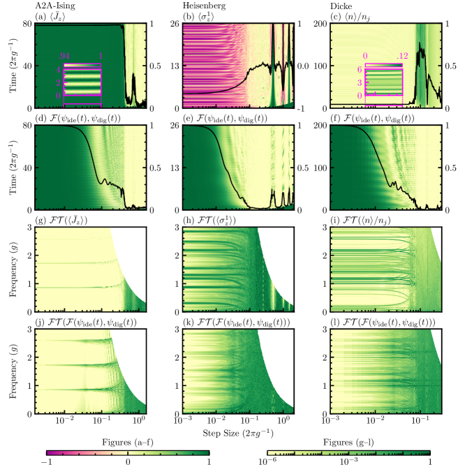
Colour plots in Fig. 3 (a–f), with the time on (the left) y-axes and the step size on x-axes, show our results for the dynamical quantities given in the titles of each sub-figure. The black lines on the colour plots are the time average of the same quantities (averaged over the full time-axis), with their y-axes given on the right side of the figures (matching the corresponding colour bar axes). The colour plots in Fig. 3 (g–l), with the frequency on y-axes and the step size on x-axes, show the Fourier transforms of the quantities plotted in Fig. 3 (a–f), as given in the titles of each sub-figure. The white regions at large step sizes in Fig. 3 (g–l) are due to the low sampling rate (Trotter step size) restricting the maximum frequency that can be resolved.
4.1.1 Destruction of Quasiperiodicity in the Dynamics of Physical Observables
In quantum simulations, we are mostly interested in studying the expectation values of some physical observables, which are typically periodic or quasiperiodic for regular quantum dynamics, and the destruction of (quasi)periodicity is a characteristic signature of quantum chaotic dynamics. Here, we show the onset of this destruction in Trotterised dynamics as the step size is increased beyond a clear threshold. Figures 3 (a–c) illustrate this effect for A2A-Ising (with ), Heisenberg (chain of qubits), and Dicke (with ) models, showing the time evolutions of the observables: (a) magnetisation—the normalised expectation value of the angular momentum operator, (b) first qubit polarization—the expectation value of the qubit-1 Pauli z-operator , and (c) normalised photon number (with based on the numerical observations discussed in the Sec. 4.2), respectively. Because the total simulation time of each model in Fig. 3 is chosen to reveal long time details of the dynamics, especially for simulation fidelities discussed in Sec. 4.1.2, some of the fast lower contrast dynamics in quasiperiodic regimes are only revealed when zoomed in. The insets in Fig. 3 show the quasiperiodic behaviour present in each model by magnifying both the temporal features and the colour contrasts.
The transition from quasiperiodic to quantum chaotic dynamics at the threshold is arguably even more pronounced in the corresponding Fourier spectra. Figures 3 (g–i) show the Fourier transform of the expectation value time traces for the same observables defined above. These clearly illustrate distinct frequency components in the dynamics before the threshold and essentially flat Fourier spectra after the threshold. Figures 3 (g–i) also provide the first indications that there are two distinct pre-threshold regimes for the quasiperiodic dynamics (which will be discussed further in relation to simulation fidelities below), defined by “branching” of the spectral frequencies once the step size is sufficiently large. Note that the vertical “lines” appearing near the threshold in Fig. 3 (g) are due to digital aliasing of high frequencies that are not properly resolved due to the low sampling rate ().
The threshold position is clear from both the destruction of quasiperiodicity and the time averages (shown in black lines) in Fig. 3 for (a) Ising and (c) Dicke models. For the Heisenberg model, however, while the full dynamics clearly exhibit a threshold, the time averages do not. The reason for this is immediately apparent from the full dynamics and corresponding spectra. Specifically, the bending of the quasiperiodic frequencies prior to the threshold washes out the time averaging and obscures the threshold, even while the full dynamics still shows a clear transition. Here, the pre-threshold behaviour is connected with initial-state-dependent Trotterisation behaviours. In Appendix D.3, we analyse the Heisenberg DQS for various classes of initial states and show that, while all the states ultimately converge to the same threshold, they show significantly varied Trotter errors prior to the threshold. Note, our results do not depend on the specific choice of operator for the expectation values or the sub-system. The first qubit of the Heisenberg chain is used only for numerical convenience, see Appendix D.2 for the other qubits in the Heisenberg chain.
4.1.2 Simulation Fidelity
In this section, we study the overall simulation performance as characterised by the simulation fidelity to the target dynamics. In previous work [46], where simulation performance was characterised through the use of time-averaged quantities, the simulation fidelity seemed to exhibit no persistent threshold behaviour. Here, however, by studying full time evolutions, we demonstrate that a clear breakdown threshold also appears at the same location in the simulation fidelity, and can explain the apparently inconsistent behaviour observed in Ref. [46].
The simulation fidelity, defined as the overlap between the states and obtained, respectively, from Trotterised and ideal dynamics,
| (24) |
directly characterises simulation performance via the error in the simulated output state. Figures 3 (d–f) respectively for A2A-Ising, Heisenberg, and Dicke models, show that the simulation fidelity is oscillatory in time before the threshold and quickly decays beyond it. This sudden change in the dynamical characteristics of simulation fidelity identifies the threshold.
Studying the simulation fidelity dynamics in more detail, however, we can identify three qualitatively distinctive regions of dynamical behaviour. Again, these observations are even more clear in the Fourier spectra in Figures 3 (j–l). In the first region of each model, at short enough times and small enough step sizes, the simulation fidelity shows a clear fast oscillation with a period that is approximately step-size independent, but an amplitude that gets deeper with increasing step size. At larger step sizes and times, the slower and larger excursions in simulation fidelity with step-size-dependent quasiperiodicity (characterised by splitting and bending frequencies in the spectra) start to dominate. Finally, at the same step-size threshold as observed in other signatures, we see a sudden (simulation-time-independent) transition from quasiperiodic fidelity dynamics to simulation fidelities that rapidly collapse with simulation time (illustrated by effectively flat spectra), an effect which becomes increasingly stark with increasing system size.
These dynamical results provide clear explanations for the trends observed in the time-averaged values in Ref. [46]. Namely, while the same sudden threshold can be observed in simulation fidelity as in other signatures, significant pre-threshold reductions in time-averaged simulation fidelity result from the increasing amplitude and complexity of quasiperiodic oscillations with both step and system sizes, to the extent that the breakdown threshold in time-averaged fidelity can even be completely obscured at larger system sizes (see also Sec. 4.2). They furthermore show that the fidelity does not irrevocably break down until after the threshold, hinting that pre-threshold errors could be significantly correctable with perturbative treatments, such as the Floquet-Magnus expansion used in Refs [45, 46] for observable expectations. This implies that, before the threshold, the states might differ only up to perturbative corrections in the Floquet-Magnus expansion for the specific Trotterisation. While outside the scope of this paper, our results highlight that a detailed study of full simulation fidelity dynamics and possible connections to perturbative error correction terms may reveal valuable new insights into the nature of Trotter errors.
Our three models cover different systems, system parameters and symmetries. Yet in terms of both the nature of the Trotterisation threshold and the nature of error perturbations in the quasiperiodic regimes, the observation and behaviour of simulation fidelity in the three qualitatively different regions shown here, remain robust across specific model and parameter choices (including across rather wide-ranging exploratory numerical analyses not presented here).
4.1.3 Stable Regions
In each model, beyond the stability threshold, we also observe clear quasiperiodic regions, as seen in Fig. 3 (and in Appendix Figs. 10 and 15), where the quantum chaotic dynamics are partially or strongly interrupted. These stable regions arise as a form of Trotterised digital aliasing. Specifically, they are localised at step sizes where the Trotterisation (sampling) frequency is sufficiently close to some underlying frequency in the Trotterised dynamics, which then effectively freezes its contribution to the Trotterised evolution. For example, in our Trotterised Heisenberg model, we observe revivals of stability at step sizes where the two-body exchange interactions freeze out: that is, for our model parameters, at for integer , where . The revivals therefore also depend explicitly on the Trotterisation recipe and product formula. The more components frozen by this sampling resonance, the stronger this effect. Because of its high parameter symmetry and simple constituent gates, our Trotterised Heisenberg model exhibits very strong revivals in comparison with those of the A2A-Ising and Dicke models. The revivals are observed much less prominently in simulation fidelity, however, because the digitisation-induced stable behaviour does not generally match the underlying, non-digitised target dynamics.
The Trotterised A2A-Ising model provides a complementary lens through which to understand the stable regions. By exploiting its equivalence to a quantum kicked top and studying its well-understood classical limit [46, 53], we are able to empirically connect the appearance of the stable regions with the re-emergence of stable islands in the phase space of the collective spin (see Appendix Sec. C.3). Again, we observe that revivals in stability do not produce an equivalent revival in simulation fidelity, with observed phase-space dynamics being very different from the original target, even within the stable region.
There are many interesting questions still to understand here, and we emphasise that these may have important implications for employing DQS in future state-of-the-art quantum computers. We plan to explore these effects in more detail in future work.
4.2 System-Size Dependence
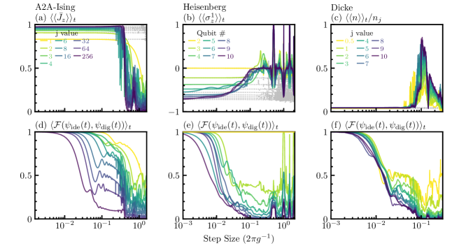
In this section, we explore how Trotterisation behaviours change as a function of system size by analysing the time averages of the dynamical quantities, and also study the smallest system sizes required to observe a distinct threshold. While we have shown that time-averaged quantities do not always show the threshold as well as their full dynamics, using the full dynamics is generally impractical for studying the dependence of Trotterisation behaviours on some other parameter such as system size. Here, with the help of the detailed understanding we have developed by studying full dynamics in the previous section, we analyse the changing behaviour of dynamical quantities with system size via their time averages, in each case from the smallest examples to dimensions orders of magnitude larger. The results (Fig. 4) show a threshold is already observable for system sizes within reach of existing experimental platforms, and that while the detailed shape of the threshold changes, its location shows minimal dependence on system size across a rather large range of Hilbert-space dimension, here limited mainly by numerics.
The target systems considered here are integrable (and therefore non-quantum chaotic). In non-integrable target systems, the Trotterisation threshold can still exist and be observable even when the target dynamics are themselves quantum chaotic irrespective of step size. (In Appendix E.4.2, we show an example in the Dicke model where the Trotterised dynamics show stronger signatures of quantum chaos after the threshold than the ideal dynamics, even when the ideal dynamics are already in the quantum chaotic regime of the model.) As discussed in Ref. [45], for non-integrable target systems, the threshold position may move to smaller step sizes for very large system sizes and run times, due to generic Floquet heating effects (see Discussion for more details). Because we consider integrable target systems, however, these observations of minimal position size-dependence are likely to hold even at very large system sizes, since the assumptions underpinning generic Floquet heating results may not apply.
It is important to note that subtle issues can arise when calculating time averages from discretely sampled time series. The light grey lines in Fig. 4 show the temporal averages for the ideal evolution sampled at equal time intervals , illustrating how undersampling (large step sizes) can cause errors in time-averaged values even for ideal dynamics. This highlights that there is a key distinction between discrete sampling errors and the Trotterisation errors, which we discuss further in Sec. 4.4. Here, we focus on the temporal averages of the Trotterised dynamics for each model:
A2A-Ising model
The first column of Fig. 4 shows the time averages of (a) values and (d) simulation fidelities for a selection of system sizes between and (labelled in Fig. 4 (a)), averaged over . Thresholds in the expectation values clearly appear around the same position for any system size considered, and at the same location as a secondary drop in the simulation fidelities which marks its transition from oscillatory to decaying behaviour. At the smallest sizes (), however, we observe neither the secondary drop in simulation fidelity, nor thresholds in the expectation values, although noticeable, smooth deviations from the ideal dynamics do occur starting around the same threshold position. In Appendix C.1, we provide the dynamical evolutions of expectation values for and observe that quasiperiodicity is only destroyed once , which is confirmed by eigenvector statistics analyses in Sec. 4.3. The threshold does not move appreciably in position with system size, and becomes sharper once the system is large enough to show quantum chaotic dynamics (in this case ). These results suggest that quantum chaotic dynamics beyond the threshold may be necessary for the system to exhibit any distinct threshold behaviour.
Heisenberg model
The second column of Fig. 4 shows the time averages of (b) values and (e) simulation fidelities for the system sizes given in the Fig. 4 (b), and for . The threshold position is still largely independent of system size, but identification of the threshold from these time-averaged quantities is more subtle, due to initial-state effects discussed in Sec. 4.1.1. In Appendix D.3, we provide the time averaging and error analyses for various types of initial states, and they confirm the fact that some initial state choices result in larger pre-threshold Trotter errors than others. In addition, for the same system sizes considered here, we also carry out eigenvector statistics analyses in Sec. 4.3, which show that global signatures of the full Trotter step unitaries (that is, averaging over all initial states) still show the same distinctive threshold. Note that there are no Trotter errors in the two-qubit case, so it has unit simulation fidelity (yellow line in Fig. 4 (e)), even though it still suffers from sampling errors at large steps.
Dicke model
The third column of Fig. 4 shows the time averages of (c) scaled values and (f) simulation fidelities for the system sizes labelled in Fig. 4 (c), and for . Here, we observe a threshold even at the smallest size , the Rabi model. In the Appendix E.1, we include the dynamical evolutions of various quantities for the Rabi model, which already show dynamical signatures suggestive of quantum chaos, such as the destruction of quasiperiodicity. Thus, we still see a distinct threshold whenever we also observe dynamical signatures of quantum chaos beyond the threshold. Surprisingly, however, in the next section, we show that the eigenvector statistics in the Sec. 4.3 do not agree with the RMT distributions for the Rabi model, with RMT agreement once again obtained only when the spin component is large enough, see Sec. 4.3 for the details. This highlights why dynamical signatures provide insufficient evidence of the presence of true quantum chaotic dynamics.
The Dicke model therefore provides a very interesting case study into what kind of system-size effects influence whether a genuine transition to quantum chaotic dynamics can be observed. Clearly, a Trotterisation threshold (and quantum chaos beyond it) can only exist when there are non-commuting terms in the Trotter decomposition. Otherwise, the decomposition would be exact and show regular dynamics for any (since we have chosen integrable target model parameters). In the Trotterised Dicke model, the non-commutation between the TC and anti-TC component unitaries in each Trotter step is introduced primarily by single-qubit gates, and not the cavity operators. This suggests that the quantum chaotic dynamics in this model is mainly driven by the spin- component Hilbert space. We further support this intuition with the numerical observations that, beyond the threshold: (a) the entropy in the spin- component is maximised (for large enough ) (Appendix B), and (b) the maximum photon numbers and participation ratio values (PR; defined in Appendix B) are, respectively, linear and quadratic in the dimension of the spin- component (Appendix E.2). This supports the notion that, despite strictly being infinite dimensional, the cavity mode Hilbert space explored by the Dicke model dynamics is effectively limited in size by the dimension of the spin. In our results, we therefore normalise the photon numbers by (Fig. 4 (c)), and the PR by ) (Appendix B), the specific coefficients ( and ) being identified empirically (see Appendix E.2). The question of how to normalise the Hilbert-space dimensionality also arises in the context of the eigenvector statistics analysis (Sec. 4.3), with results consistent with the somewhat empirical approach taken here.
4.3 Eigenvector Statistics
In this section, we analyse the static properties of a Trotterised evolution, namely the eigenvector statistics of the Trotter step unitary. So far, we have employed time evolutions and averages of dynamical quantities to show a range of Trotterisation behaviours, including the threshold, low system-size dependence, and dynamical signatures of quantum chaos beyond the threshold. These dynamical analyses, however, are generally neither conclusive nor global. That is, they are not able to provide unambiguous evidence of quantum chaotic Trotterised evolution without relying on additional random matrix theory (RMT) analysis, nor do they readily enable conclusions about Trotterised evolution across the full system Hilbert space. Here, using eigenvector statistics, we demonstrate conclusive agreement with the predictions of quantum chaotic dynamics beyond the threshold, and since this approach probes properties of the full Trotterised unitary, it provides information about the global dynamics in a manner insensitive to initial-state choice.
4.3.1 Goodness-of-Fit Test for Eigenvector Statistics
Dynamical signatures of quantum chaos are fundamentally consequences of the random matrix theory (RMT) properties of the eigenvectors and eigenvalues of a quantum chaotic system [53], known respectively as eigenvector [55, 56] and level-spacing statistics [87, 88] (see Appendix A for further details). Reference [46] explored the level-spacing (eigenvalue) statistics through the mean eigenphase-spacing ratio, and a participation ratio derived from eigenvector statistics. Unfortunately, these averaged and derived quantities do not unambiguously identify the presence (or absence) or quantum chaos for a particular Trotterised step unitary, without appealing to other model-specific information, which may or may not be available. For example, for their particular Trotterised A2A-Ising model, Ref. [46] was able to exploit its well-understood classical limit as a kicked top, an approach which is obviously not available in general.
In this work, we instead carry out the comparison against RMT statistics at the full-distribution level. Furthermore, we focus on eigenvector statistics, because while it may be more straightforward to measure level spacings directly in natural quantum systems, this is generally not also true for quantum simulators, and unlike with eigenvectors, there is no generic closed-form solution for calculating the expected statistics for RMT level spacings (see Appendix A). In experimental quantum simulators, spectral information gained via Fourier transform and Ramsey-like measurements can provide access to eigenvalue statistics [89], and recent theory work has begun exploring ways to probe both eigenvalue and eigenvector statistics via the spectral form factor [90, 91].
While this is not the first time the RMT properties of physical models have been studied at the full-distribution level, we demonstrate that the usual approach of making a visual comparison of the eigenvector statistics against the above RMT distribution can be misleading. We overcome this problem by combining the eigenvector statistics with a reduced chi-squared goodness-of-fit test, and use a reduced chi-squared goodness-of-fit test statistic, , to clearly and objectively demonstrate the onset of quantum chaos in the Trotterised dynamics both as a function of step and system sizes. As a measure of full distribution-level agreement, provides an objective statistical RMT comparison for arbitrary, individual unitary matrices, and avoids the ambiguities that may arise when relying on individual distribution moments.
Here, we calculate the eigenvector statistics of the Trotter step unitary (TSU), , by expanding its eigenvectors in a basis , defined by the eigenvectors of the free Hamiltonian (i.e., without the coupling terms ) in each model. The squared moduli of complex coefficients then show certain distributions for quantum chaotic systems [55, 56, 92]. Depending on the time-reversal symmetry of the system, there arise three (main) physically relevant random matrix ensembles [93], known for random unitaries as the circular-orthogonal ensemble (COE), circular-unitary ensemble (CUE), and circular-symplectic ensemble (CSE). Their corresponding reduced probability densities are:
| (25) | |||||
| (26) | |||||
| (27) |
where is the dimension of the Hilbert space, and is the Gamma function, or generalized factorial. We denote these distributions in our figures by the above three letter acronyms of the corresponding classes. Relevant details about these distributions, the choice of basis , the relation between RMT and quantum chaos, and other technical factors are summarised in the Appendix A.
4.3.2 Failure of visual comparisons versus
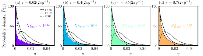
Figure 5 shows the eigenvector statistics of the A2A-Ising TSU calculated in the basis for . Figures 5 (a–d) are, respectively, for the step sizes from (a) before the threshold, (b) on the threshold, (c) in the quantum chaotic regime beyond the threshold, and (d) on a stable region in the quantum chaotic regime. Note that collective spin behaviour in the A2A-Ising DQS restricts the system evolution into a total-spin conserved subspace of the full Hilbert space of spin-1/2 systems. In this respect, it does not display many-body quantum chaos of systems but quantum chaos of a single spin , and the standard RMT distributions in Fig. 5 are for . Because the A2A-Ising decomposition in Eq. (8) has only time-reversal symmetry, it should show COE statistics [46]. While Figure 5 (a/c) shows clear visual disagreement/agreement with the expected COE distribution, the apparent visual agreement in Fig. 5 (d) is highly misleading, as this corresponds to a stable region, where the quantum chaotic dynamics are definitely interrupted. To characterise this agreement in a more quantitative manner, we introduce a reduced-chi-squared goodness-of-fit test statistic to provide a generic quantitative signature for the agreement with the eigenvector statistics expected for random matrix theory (see Appendix A.3 for the definition and more details). The values of comparing the histogram plots with the relevant COE distribution in Figs 5 (a–d) are, respectively, (a) , (b) , (c) , and (d) , successfully identifying not only the agreement/disagreement in regular/quantum-chaotic regime, but also the significant disagreement within the stable region. For Figure 5 (b), which arguably also agrees reasonably well visually, the demonstrates even stronger disagreement with the target COE distribution.
In general, RMT can be used to make specific quantitative predictions about the expected distributions of eigenvector coefficients for random unitary matrices, but does not provide any guidance as to the eigenvector distributions expected for non-random matrices. Similarly, the goodness-of-fit test enables quantitatively rigorous analysis of whether the observed distribution for a particular unitary is consistent/inconsistent with the distribution predicted by RMT, with the general guide that agreement requires . However, while definitively rules out agreement with a particular model, the goodness-of-fit test makes no prediction about what should be in the case of disagreement. In these results, can take on very large values where the models do not agree with RMT, as a result of exponentially small values in the large- tail of the predicted RMT distributions. Thus, the presence of localised (non-random) eigenstates (with large ) makes exponentially large contributions to . While this effect can be seen slightly more clearly by replotting the data from Figs 5 (a–d) up to in logarithmic -scale, there is still minimal visually clear distinguishability between Figs 5 (b–d). Therefore, our new metric provides an important first step in the development of objective measures for identifying RMT, which we will study further in future work.
The goodness-of-fit test statistic provides a single and (compared to visual inspection) meaningful value for a histogram plot, and therefore also allows us to analyse the eigenvector statistics as a function of some parameter. In the following, we provide the analyses of eigenvector statistics for the Trotter step unitaries of each DQS as a function of step and system sizes. Full eigenvector statistics histograms for some relevant step and system sizes are shown in Appendix C.2 for A2A-Ising, in Appendix D.1 for Heisenberg, and in Appendix E.3 for Dicke Trotterisations. Note that values for the Dicke DQS are obtained by setting the cavity truncation to , and we discuss this further after presenting the results.
4.3.3 Onset of Quantum Chaos as the Trotter Step Size Increases
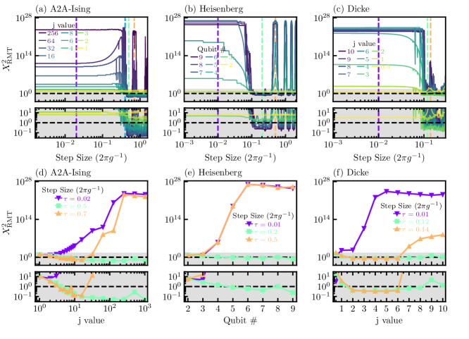
Figure 6 (a–c) shows the test statistic as a function of step size, respectively, for (a) the A2A-Ising TSU (against COE), (b) the Heisenberg TSU (against CUE), and (c) the Dicke TSU (against COE). In each model, shows a sudden drop to for system sizes larger than a certain value that depends on the model, demonstrating good agreement beyond this point between the eigenvector statistics of these TSUs and the corresponding RMT distribution, and providing strong, objective evidence of quantum chaotic dynamics. These results illustrate that each of these models undergo a dramatic transition from regular to quantum chaotic dynamics at a position that matches the threshold identified from dynamical signatures, and which sets in already at quite modest system sizes. Across all models and multiple orders of magnitude in Hilbert-space dimension, once the system reaches sufficient size, we do not observe any significant variation with system size of the position of onset for .
4.3.4 Onset of Quantum Chaos as the System Size Increases
Here, we examine as a function of system size for three indicative step sizes in the regular (pre-threshold), quantum-chaotic (beyond-threshold), and stable-revival regions. Figures 6 (d–f) plot this dependence for (d) A2A-Ising TSU (against COE), (e) Heisenberg TSU (against CUE), and (f) Dicke TSU (against COE), respectively, for the step sizes given in each legend. Before the threshold, is much larger than 1 in every DQS and any system size considered. This means that, as expected, the eigenvectors do not show RMT properties before the threshold, and the DQS is quasiperiodic (non-quantum chaotic) for these step sizes. By contrast, rapidly drops below 1 for the quantum chaotic regime of each model as the system size increases. The bottom panels showing a zoomed-in view of the grey shaded regions where show clearly at what size each system’s TSU starts to agree convincingly with RMT predictions in its quantum chaotic regime: namely, for in A2A-Ising, for in Heisenberg, and for in Dicke Trotterisations, respectively. Figures 6 (d–f) also show that rapidly increases to values much greater than 1 for step sizes in the stable regions, which appear at any system size in the Heisenberg DQS, and emerge at larger sizes in the A2A-Ising and Rabi-Dicke models.
4.3.5 Finite Truncation of the Cavity Dimension in the Rabi-Dicke DQS
Similar to the A2A-Ising DQS, the Dicke DQS also consists of a mapping from spin-1/2 systems to a single total spin . Below, we argue that, as a result of the single-qubit gates in the Dicke Trotterisation, the effective total spin component of the model is the main driver of quantum chaotic dynamics. However, there are additional complications in the eigenvector statistics analyses of the Dicke TSU that arise from numerically truncating the infinite-dimensional cavity at a finite value . It is non-trivial and is not in the scope of this paper to provide a rigorous, theoretical explanation of the effects of cavity Hilbert-space truncation on eigenvector statistics, but, in Appendix E.3, we study it in some detail numerically. Complementing the eigenvector statistics with another strong signature of quantum chaos from RMT, the level-spacing statistics [88, 87, 54, 53], we observe that the beyond-threshold Dicke TSUs show agreement with RMT distributions only for , both for eigenvector and level-spacing statistics. Any agreement is lost simultaneously in both of these statistics when . Combined with the dynamical observations that maximum photon build-up is linear in , and the PR is quadratic in (and the fact that the reduced entropy of the spin subsystem is nearly maximised), these results indicate that quantum chaotic dynamics and Trotterisation breakdown in the Dicke model are primarily driven from effects arising within the Hilbert space of the spin component.
4.4 Trotter Error Analyses
In each model, by analysing the statistical properties of the Trotter step unitary and temporal evolutions (and averages) of various dynamical quantities, we have identified a range of apparently universal performance behaviours and a threshold in Trotter step size beyond which the Trotterised dynamics become quantum chaotic. Here, we analyse the Trotterisation errors in state fidelities and expectation values, and we identify the same threshold in each error measure and also examine the behaviour of the errors before and beyond the threshold. We look at the Trotter errors for various system sizes and different time scales: The shorter time scales considered can be achieved within accessible coherence times for current experimental platforms, demonstrating that studies of Trotter-error scaling with step size are within reach of current experiments.
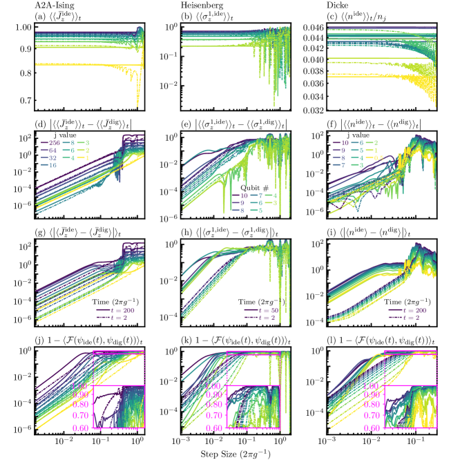
Figure 7 shows our error analysis for the A2A-Ising, Heisenberg, and Dicke models. We first analyse errors in the expectation values of local observables, using the same observables considered in previous sections. The results in Figs 7 (a–c) highlight an important subtlety: namely, even for ideal dynamics, sampling the time evolution at fixed times can lead to errors in time averages at large enough . These time averages also depend strongly on the averaging time, with more pronounced errors arising at smaller step sizes for short averaging times. Such undersampling errors obviously become more significant with a lower sampling rate. Here, we introduce appropriate error measures to distinguish trivial sampling errors from the approximation errors caused by Trotterisation.
We start by considering the absolute difference between the temporal averages (as previously studied in Ref. [46])
| (28) |
where is the expectation value of some operator , with the superscripts (dig/ide) indicating expectation values obtained, respectively, from digital and ideal dynamics (sampled at every ), and the second layer of brackets represent time averaging for total simulation time . Figures 7 (d–f) show for each model. In each model, shows an approximately increasing trend with step size leading up to the previously identified threshold positions, before flattening out after the thresholds. (Note that the error values for the expectations in Ising and photon numbers in Dicke are not normalised with spin sizes to avoid removal of system size dependencies in the errors.) In the A2A-Ising model (Fig. 7 (d)), the errors reveal a reasonably clear threshold at the right position, although this is somewhat complicated by the appearance of additional noise prior to the threshold. In the Heisenberg and Rabi-Dicke models (Fig. 7 (e–f)), the situation becomes much less clear, with significant extra noise before and after the threshold, and clear irregular behaviour even at small . Moreover, while still shows a generally increasing trend with step size, it does not show an obvious scaling dependence with system size and/or total simulation time across any of the models. So even though this measure does to some degree attempt to isolate the effect of Trotter errors from sampling errors, it nevertheless does not provide a good error measure for identifying differences between Trotterised and ideal time evolutions, especially at the finite times relevant to practical DQS. For example, a small difference between the averages does not guarantee that the instantaneous time evolutions are actually close.
We therefore introduce and analyse an alternative time-averaged error, namely the average, point-to-point absolute difference between expectation values
| (29) |
where the notation is the same as in Eq. (28). Now, captures the absolute deviations of Trotterised evolution from the ideal dynamics at every sample, and is only zero for identical trajectories. It therefore both separates the Trotter errors from sampling errors, and reliably measures how close the full dynamical evolutions are (not just their averages). From Figs 7 (g–i), unlike for , we observe that is a simple analytic function of step size over a large range of step sizes (prior to a plateau region that appears at long time averages), suggesting that it can be perturbatively expanded (and potentially corrected) in step size, even at point-by-point detail for finite-time evolution. Similarly, it also shows a clear increasing trend not only with step size, but also as a function of both total simulation time and, with some subtle variation, system size. From Figs 7 (g–i), we see that the average, point-to-point error also shows the thresholds much more clearly, especially in the A2A-Ising and Rabi-Dicke models, with the errors before the threshold being consistently smaller than the errors in the quantum chaotic regime. Even in the Heisenberg model, where the near-threshold errors almost reach the levels observed in the quantum chaotic regime, the errors still show a clear change in step-size scaling beyond the threshold.
Another averaged, point-to-point error measure is the averaged simulation (state) infidelity (or simulation error) , shown in Figs 7 (j–l), and it shows the same behaviours observed in . The lack of a sharp threshold in average simulation error has already been explained in the context of average fidelity as the result of the extra oscillatory behaviour of simulation fidelity before the threshold. Consistently, it affects the long time averages much more than the short, and we identify the threshold as the residual, secondary jump in simulation errors highlighted by the insets of Figs 7 (j–l).
5 Discussion and Outlook
The power of a quantum simulator, as represented by the achievable complexity of tasks that it can solve, is typically limited by physical resources (e.g., fabrication costs or runnings costs per qubit, cooling budget per qubit), hardware performance (e.g., qubit noise and decoherence, gate errors, etc), and in the case of DQS, the intrinsic accuracy of the digitisation algorithm (e.g., Trotter errors). In large-scale quantum simulators, these resource costs will be to some degree fungible, and balancing them will become an engineering optimisation to maximise simulation power. For example, in fault-tolerant DQS, error correction will ultimately allow hardware performance limits to be surpassed by transferring the cost into increased consumption of physical resources. But because these costs snowball as the noise to be corrected approaches the fault-tolerant threshold, directly optimising hardware performance will still remain crucial. Similarly, methods for improving digitisation accuracy typically result in increased exposure to noise and decoherence. For example, in architectures where gate times operate reasonably close to the speed of the control electronics, the total run time (and hence decoherence effects) can be increased because the time spent on buffers between gates can be significant. Also, constructing complex interactions from simple primitive operations often requires additional transformation gates (e.g., as in the Heisenberg and Dicke models defined in Eqs 14 and 23, respectively), adding both run time and gate errors. Similarly, increasing the order in Trotterisation algorithms, which typically requires the addition of negative-time unitary evolutions (at least beyond second order), also increases the laboratory run time required to achieve a given simulation time. As a result, any improvements that can be achieved in terms of relaxing the digitisation requirements for a given simulation accuracy, will also directly decrease the decoherence and gate errors experienced by the processor.
5.1 On the universality of Trotterisation performance
In this work, we have focussed exclusively on digitisation errors, in particular Trotter errors, to study the ultimate performance limits that Trotterisation algorithms will face. We numerically investigate the performance of three experimentally realisable Trotterisation models: the A2A-Ising, Heisenberg, and Dicke models. Using a range of dynamical and static signatures (derived from state evolutions and unitary operators, respectively), we have demonstrated a marked degree of universality across DQS models for a range of performance behaviours, including the emergence of a performance threshold at modest system sizes, which is observable across all signatures we studied. Firstly, the full dynamics (Figs 3 (a–c)) and time averages (4 (a–c)) of local observables, delocalisation and other complementary derived quantities (Fig. 10 in Appendix B), and new static signatures of quantum chaos based on RMT (Fig. 6), show that, once a sufficiently large system size is reached, all models studied exhibit regular, quasiperiodic behaviour prior to, and quantum chaotic dynamics after the threshold. However, in addition to just the threshold, by studying in detail the full dynamics of the simulation fidelity (Figs 3 (d–f)), we demonstrate that the widely different models considered also exhibit a broader range of shared behaviours: a high-fidelity region at smaller steps and shorter times, with fast, but relatively stable oscillatory errors; a second region between that and the threshold exhibiting additional, slower large-amplitude oscillations; and, within the post-threshold quantum chaotic regime, intermittently emerging stable regions where the quantum chaotic dynamics is interrupted and some degree of quasiperiodicity reemerges. These new shared behaviours, as well as the threshold itself, become arguably even more apparent from studying the corresponding Fourier spectra (Figs 3 (g–l)).
The models studied here encompass widely distinct system types and symmetries (kicked tops, nearest-neighbour spin chains with longitudinal and transverse external fields, and coupled spin-cavity systems with infinite dimension), and we also saw qualitatively similar behaviour across different parameter choices (not shown). The marked universality of all behaviours suggests that there may exist underlying generic principles governing the behaviour of Trotterised DQS, which may help to predict features of large-scale simulations which are difficult to study classically. More work is required to identify and understand these underlying principles. Interesting open questions in this direction include, for example, studying whether these generic behaviours persist for different digitisation techniques, even more varied simulation models (e.g., in quantum chemistry), and non-integrable target systems.
5.2 On interpretation of the Trotterisation threshold
Focussing now directly on the threshold transition to quantum chaos, combining what we learn from across all our results provides valuable insight into the underlying nature of the breakdown in simulation performance. From the full dynamics for each model (Fig. 3), we observe clear quasiperiodic dynamics, consistent with the Trotterised system being non-quantum-chaotic, until immediately prior to the threshold (given in units of : , and ). The pre-threshold oscillatory behaviour is particular clear and sudden for the local observables (Fig. 3 (a–c)) (and the participation ratio (Fig. 10 (a–c)) in the Appendix B). For the simulation fidelity in Fig. 3 (d–f) (and the perturbation fidelity (Fig. 10 (d)) and entropy of entanglement (Fig. 10 (e–f)) in the Appendix B), the periodicity of the oscillations starts changing prior to the threshold (as seen in the Fourier transform shown in Fig. 3 (g–l)), but clear oscillations continue until the threshold. This understanding is also consistent with the Trotter error analysis shown in Fig. 7, and particularly the full quantum state error calculated from the simulation fidelities Fig. 7 (j–l). Focussing on the plots with shorter time averaging, where the simulation-fidelity time averages are less complicated by the behaviour in the near-threshold, quasiperiodic region, we observe that the full quantum state errors follow an analytic, increasing trend up until just prior to the threshold. In other words, the Trotter error grows steadily with step size, which matches the intuition suggested by considering the Trotterised (Floquet) Hamiltonian as a convergent Floquet-Magnus expansion, with the zeroth-order solution reproducing the target dynamics and perturbatively increasing correction terms [45, 46]. And while the errors (state infidelity) may still become significant in this region, they are in some sense still well behaved: from a given step size, you can expect to improve performance by reducing the step size, and worsen performance by increasing it. This provides crucial support to the notion that, prior to the threshold, the Trotterised model implements a meaningful and controllable approximation of the underlying target dynamics.
Beyond the threshold, our new model-agnostic, objective static signatures based on eigenvector statistics (Fig. 6) demonstrate that, once the system is large enough, the Trotter step unitary shows strong quantitative agreement with RMT distributions. This provides strong, quantitatively rigorous evidence that the Trotterised dynamics become quantum chaotic beyond the threshold. And since we chose target systems and parameters corresponding to integrable dynamics, we know that it is not the target dynamics ( in Eq. (5)), but the increasingly dominant Trotter errors that give rise to the observed quantum chaos. But if the Trotter step unitary becomes a completely random matrix, the intuition of Trotterised DQS as approximate simulation of one particular target model breaks down entirely, since its behaviour (within a local region of step size) is no more consistent with one model than any other (subject to underlying symmetries). This combination of results shows how we can make a direct connection between the onset of digitisation-induced quantum chaotic behaviour in DQS and the empirical breakdown in meaningful simulation performance. And while we do not make any rigorous connection between this threshold and the formal radius of convergence in the corresponding Floquet-Magnus expansion, we nevertheless identify the quantum chaotic threshold as an emergent radius of convergence for simulation performance.
Here, it is worth noting again the importance of introducing the goodness-of-fit test statistic as an objective, quantitative measure of likelihood that an individual Trotter step unitary belongs to a given class of random unitary matrices. As discussed in Sec. 4.3 and illustrated in Fig. 5, the visual comparisons usually applied to identify distribution-level agreement with RMT predictions are completely inadequate to reliably and accurately identify whether genuine agreement is present. This work establishes the use of statistically rigorous, full-distribution comparison techniques as a valuable new approach for developing better ways to study random matrices and quantum chaotic dynamics through eigenvector and eigenvalue statistics. This has important applications across various areas of quantum physics, including quantum computing. Yet there are many important open questions. For example, while exploring the ideal (non-Trotterised) Dicke model to find operating parameters giving regular dynamics, we found regimes where good visual agreement could be identified with eigenvalue statistics, but not with eigenvector statistics. In such cases, which signature, if either, can be considered to be more definitive? And while using has already provided significant value and insight for this work, what is the optimal statistical approach to take?
5.3 On size dependence of the threshold
From the time-averaged dynamical signatures studied in Figs 4 and 7, we see that neither the threshold nor the characteristics of quantum chaotic dynamics are observed at the smallest system sizes for the A2A-Ising and Heisenberg models. These only emerge once the system is large enough ( for A2A-Ising, see also Appendix Fig. 11, and for Heisenberg), and the same size is observed for the onset of quantum chaos as identified by quantitatively rigorous agreement with RMT (Fig. 6, see also Appendix Figs 12 and 13). For the Rabi-Dicke model, however, the threshold and dynamical signatures of quantum chaos are visible even at the smallest system sizes (one qubit and one cavity, see Appendix Fig. 17), yet quantum chaotic behaviour as characterised by agreement with RMT is still only observed for large enough spin dimensions. While the exact reason for this different behaviour is still an open question, we speculate that this may arise from the presence of the infinite-dimensional cavity in the Rabi-Dicke system.
In the context of DQS, Trotterisation can be interpreted as implementing a periodically driven, time-dependent Hamiltonian, and the digitised dynamics understood in terms of an effective Floquet Hamiltonian [45, 46]. As discussed in Sec. 2, the Floquet-Magnus approximation in the general case breaks down beyond a formal radius of convergence , and the inverse scaling of a rigorous sufficient condition for convergence with system size [62, 63, 64] (if tight) would imply that realising accurate simulations for very large systems could require vanishingly small Trotter step sizes. This could have significant, fundamental implications for the practicality of future large-scale DQS, but results from recent works [45, 46, 65] do not appear to conform to these expectations. We have extended the work on this issue, in terms of the range of both models and characterisation tools, and have seen minimal if any movement of the threshold, certainly much less than the almost 3 orders of magnitude variation in Hilbert space size studied. Indeed, the threshold arguably becomes more fixed in position as size increases, with possible movement observed more at low system sizes where the thresholds are less sudden and harder to locate precisely. These observations seem to contradict the expectation that for the radius of convergence of the Floquet-Magnus expansion.
Recent asymptotic results from Floquet physics [58, 59, 60, 61] suggest that any sufficiently generic, fixed, interacting quantum many-body system, when subjected to periodic driving, will heat up indefinitely, which is a signature of quantum chaotic dynamics. Thus, in the thermodynamic size limit and asymptotically long times, generic Trotterised DQS may also exhibit quantum-chaos-driven heating, which suggests that a quantum-chaotic breakdown in simulated dynamics may already be observed for step sizes smaller than thresholds identified at short times. It is not yet understood what system sizes will bring these heating effects into play, but as already noted in Refs [45, 46], this heating takes place exponentially slowly in the fast driving regime which usually characterises a DQS operating in the pre-threshold regime. It therefore seems likely that the universal Trotterisation behaviours observed here will continue to be relevant for sizes and times applicable to NISQ-era and early fault-tolerant processors, where error mitigation and resource optimisation will be so critical. And even if systems and run times do eventually reach large enough scales, they can still be exponentially suppressed by increased digitisation. That is, for specific, long, yet finite simulation times, the Trotterisation threshold can persist even in the thermodynamic limit, because heating will only become effective for large enough .
Our work also raises a number of interesting open questions in this area of asymptotic heating and Trotterisation thresholds. In the context of quantum many-body physics, sufficiently generic systems are, with vanishingly infrequent exceptions, non-integrable (or quantum chaotic). For integrable systems, however, which occur with measure zero and arise from fine-tuning of system parameters and symmetries, the asymptotic heating results [58, 59, 60, 61] do not necessarily hold [65]. In this work, to focus on digitisation-induced quantum chaos, we specifically considered systems and parameters which remain integrable even for very large system sizes. Such systems may support a full performance threshold for Trotter errors even in the thermodynamic limit. This obviously needs to be studied in more detail, but such a result, even if it does not hold completely universally, would provide valuable evidence that DQS can be carried out reliably, even at very large scales, which will be critical, if future large-scale quantum computers are to realise the promising applications of most interest. Another very important point is that these asymptotic heating results have only been studied in the context of systems with bound energy spectra, like networks of spins or fermions. It is a completely open question what might happen for systems involving bosonic degrees of freedom, which give rise to very different phenomena under periodic driving, such as parametric resonance. Systems like the Rabi-Dicke model considered here could provide interesting testbeds for exploring these questions, with potential implications for both fundamental physics and quantum processors utilising bosonic degrees of freedom.
Finally, at a more practical level, while the threshold behaviours studied in this work are visually quite clear, an important open challenge for understanding the size dependence of the threshold is to develop an objective quantitative description of where the threshold sits. Our test statistic provides a promising way to attack this problem, since it captures a direct quantitative measure of agreement with RMT in a single number, but a number of subtleties in how to identify the threshold make this an important open question for future work. For example, while the thresholds observed in in Fig. 6 are relatively sudden, and get sharper with increasing system size, they still appear to span a small finite region in step size, broader than is observed in the full dynamics. Further study of these effects are required, but we speculate this may arise because is defined from the global unitary. That is, it would be consistent with the notion of mixed-phase regions in phase space, well known in the context of the kicked top [46, 22], for the position of the chaotic threshold to show some dependence on system initial state. Indeed, it would not be surprising for such an effect to be quite significant, although some initial explorations of this possibility for the Heisenberg model in Appendix Fig. 14 observed a rather stable threshold. Also, while a goodness-of-fit test statistic value of is known to indicate good agreement with the target probability distribution, values greater than 1 do not uniquely specify the manner of disagreement. Further study is therefore required to understand whether there is a way to identify the smallest step sizes where the threshold starts. Finally, we observe that appears to exhibit some strong sensitivity to step size near the Trotterisation threshold, which would be intuitively consistent with the known sensitivity of quantum chaotic dynamics to Hamiltonian perturbations. Pronounced mainly during the narrow threshold transition, this effect creates some ambiguity in identifying a single, precise threshold. Finding a better understanding of the detailed nature of the quantum chaos transition and an objective way to precisely describe the threshold position are important open topics for future DQS research.
5.4 On scaling of Trotter errors with step size
Ultimately, resource optimisation is the goal that motivates most theoretical DQS research. A key driver for our work is that a better understanding of the detailed behaviour of Trotter errors in the pre-threshold regime most relevant for useful DQS may allow advanced quantum processors to maximise computational capacity by better balancing Trotter errors against the effects of decoherence and gate noise. References [45, 46] show, at least for specific cases in the Ising model, that certain error signatures for observables agree pre-threshold with the values predicted by a perturbative Floquet-Magnus expansion of the system dynamics. Rather surprisingly, however, the specific signatures studied in these works did not generally show any clear scaling of errors with other system parameters such as size or simulation time, suggesting a rather striking difference in behaviour between errors in local observables and state fidelity signatures calculated from the full quantum state. In Fig. 7, we broaden the observation that observables errors are perturbative functions of step size to a range of different models. We also show, however, that well-defined, point-to-point errors (Figs 7 (g–l)) do indeed scale sensibly with both system size and simulation time, showing they remain controllable across all models up to just prior the quantum chaotic threshold, and are also quite consistent with observed state fidelity scalings. Indeed, by identifying two distinct behavioural regimes in the pre-threshold dynamics (Fig. 3), we identify a DQS performance region in which the simulation error (global state infidelity) can be expected to also show well-behaved perturbative scaling with Trotter step size, and our Fourier analysis of the full fidelity dynamics highlights an interest avenue for pursuing a better understanding of the underlying cause of these pre-threshold behaviours. As suggested first in [45], this means that measuring results for a range of larger step sizes can potentially allow more accurate values to be predicted by extrapolating the observations back to smaller step sizes, which then don’t need to be measured explicitly. Furthermore, provided these errors can be explained perturbatively, calculating the correction terms in a perturbative expansion like the Floquet-Magnus expansion may provide insight into how to correct these errors at an algorithmic level, to further compensate and reduce the observed Trotter errors without moving to smaller Trotter step sizes. Critical to these new observations was the introduction of more nuanced time-averaged errors that distinguished reliably between sampling errors and Trotter errors, and identify all real dynamical errors that do not always show up in infinite-time or different time-averaged error signatures. An interesting open question that requires further investigation is why, in some models, the longer-time Trotter errors appear to saturate to a finite error considerably below the value saturated by quantum chaotic dynamics beyond the threshold.
5.5 Towards experiments and potential applications
In future work, and especially in the design of future experiments, it will also be important to study the interplay between Trotter errors and noise. At the simplest level, to be able to experimentally observe the onset of quantum chaotic dynamics at the Trotterisation threshold, the decay and dephasing times will need to be significantly longer than the quantum chaotic collapse time. For the strongly quantum chaotic systems demonstrated here, this occurs already after very few Trotter steps (Fig. 3), but to distinguish this reliably from quasiperiodic dynamics in the regular (pre-threshold) regime, it will obviously be necessary to observe coherent dynamics over a longer duration. In this context, decoherence can be modelled straightforwardly using a traditional master equation in the “lab frame” of the simulator system, and simple initialisation and measurement errors can be modelled heuristically via appropriate choices of starting states and measurements POVMs. By contrast, simple gate errors such as calibration errors and parameter drift errors can be modelled using random noise parameters and Monte-Carlo techniques. The effects of gate errors, however, can be expected to raise more subtle questions for future study, since hardware errors such as gate errors and residual couplings can already lead to quantum chaotic dynamics [94, 95, 96, 97, 98, 99], even in analogue quantum systems. Note that, based on our work in this paper, some experimental results previously observed in Ref. [16] for the quantum Rabi model, can be interpreted as providing preliminary experimental verifications of our new results, indicating that the performance required to investigate these effects is already within reach of current experiments.
5.6 The broader role of Random Matrix Theory
In this work, use of random matrix theory has been crucial in establishing quantum chaos as the underlying universal (across models) and global (throughout Hilbert space) cause of the Trotterisation performance breakdown threshold first noticed in the context of Ising DQS in Refs [45, 46]. Here, it is worth putting this in the context of how RMT is also arising in other areas of quantum information. In recent years, the classical computational complexity of the random matrices underpinning quantum chaos [51] has motivated a range of pioneering experiments designed to implement random unitary circuits, like quantum supremacy and information scrambling [47, 48, 49, 50, 100, 101]. For example, in contrast to our main results, where target models are explicitly integrable and quantum chaotic dynamics arise from simulation errors, quantum supremacy experiments target the accurate simulation of quantum chaotic target dynamics specifically because it pushes the classical complexity. This provides further motivation for many open questions around how to optimise DQS of a target model which is itself quantum chaotic, a situation which is likely to arise often in real DQS applications. In Appendix E.4.2, we note already that Trotterisation thresholds may still be observable for quantum chaotic target models, but quantum supremacy experiments illustrate that this context merits much more detailed investigation. For example, does the universality of Trotterisation performance across system types observed here extend to Trotterisations of quantum chaotic target models? Do similar thresholds appear in other contexts where hardware-error-induced quantum chaos appears [94, 95, 96, 97, 98, 99], and (how) are these situations connected? We anticipate that the new analytical tools we have introduced, like the goodness-of-fit test statistic , will provide invaluable insight into such questions.
In a different direction, while we can connect pre-threshold Trotter errors to perturbative corrections in the Floquet-Magnus expansion [45, 46] and identify the threshold as an emergent radius of convergence, it remains an open question to find some mechanistic origin for the threshold and the onset of quantum chaotic dynamics beyond it. Given the key role of RMT in establishing the classical computational complexity of quantum supremacy experiments [47, 51], we suggest that RMT could perhaps be used to build an information theoretic understanding of the breakdown of DQS performance in terms of computational complexity.
Finally, in this work, we show that digitisation-induced quantum chaotic dynamics can be realised in quite modestly sized systems. While this heralds a breakdown in performance in DQS, it is intriguing to speculate whether this can be used as a resource in other contexts, such as open-system simulations (using the deep connection between quantum chaos and thermalisation in closed quantum systems [102, 103, 54]), or quantum metrology [104].
6 Acknowledgments
Authors thanks G. J. Milburn, R. L. Mann, M. J. Bremner, A. Manatuly, K. Modi, D. Braak, J. F. Ralph, and D. W. Berry for useful discussions. Numerical simulations are realised using a Python library, called QuanGuru [105], developed in our group at UTS. The data and the Python code that support the findings of this study are available from the corresponding authors upon reasonable request.
This work has been funded by the Australian Research Council Future Fellowship of N.K.L. (FT170100399). C.K. and F.H. acknowledge the supports from UTS President’s scholarship, international research scholarship, and Sydney Quantum Academy. J.P.D acknowledges support from the University of Technology Sydney, Chancellor’s Postdoctoral Research Fellowship (UTS, CPRDF). L.M.S. acknowledges support from the Austrian Science Fund (FWF): P 33741-N. P.H. acknowledges support from Provincia Autonoma di Trento, the ERC Starting Grant StrEnQTh (project ID 804305), the Google Research Scholar Award ProGauge. This project has benefited from Q@TN, the joint lab between University of Trento, FBK-Fondazione Bruno Kessler, INFN-National Institute for Nuclear Physics and CNR- National Research Council. M.H. and P.Z. both acknowledge funding from the European Research Council (ERC) under the European Union’s Horizon 2020 research and innovation programme, under grant agreements No. 853443 and No. 817482 (Pasquans), respectively. M.H. also acknowledges support by the Deutsche Forschungsgemeinschaft (DFG) via the Gottfried Wilhelm Leibniz Prize program. P.Z. also acknowledges support by the Simons Collaboration on Ultra-Quantum Matter, which is a grant from the Simons Foundation (651440, P.Z.).
Appendix A Random Matrix Theory and Quantum Chaos
Dynamical signatures of quantum chaos are manifestations of certain random matrix properties in the eigenvectors of quantum chaotic systems. Here, we provide an overview of quantum chaos and its relation with random matrix theory (RMT). We also discuss the technical subtleties and nuances involved in the calculation of the quantum chaos signatures used in this paper, and we use quantum kicked-top models of different symmetries to explain these for both statistical and dynamical signatures.
A.1 Random Matrix
A random matrix has all or most of its entries as independent random numbers satisfying certain probability laws, and random matrix theory is concerned with the statistical properties of (all or a few of) the eigenvalues and eigenvectors of such matrices. Wigner used RMT analyses to explain certain spectral properties of heavy nuclei [106], motivating much subsequent theoretical work , and Dyson showed that physically relevant random matrices fall (mainly) into one of three universality classes according to their symmetries [93]. These classes are categorised into circular or Gaussian ensembles for unitary and Hermitian random matrices, respectively. Ensembles are categorised according to the Dyson parameter into orthogonal (COE/GOE, ), unitary (CUE/GUE, ) and symplectic (CSE/GSE, ), related to degrees of freedom in random entries and degeneracies of the matrices [56].
A.2 Quantum Spectra of Classically Chaotic Systems
Over the years, many studies connected RMT with quantum chaos [88, 87, 55, 56, 54, 53], by showing that the distribution of energy levels in the Hamiltonians of classically chaotic systems, commonly referred to as the eigenvalue or level (spacing) statistics, adhere to the Wigner-Dyson statistics [87, 54, 53], given by
| (30) |
where s is the spacing between neighbouring levels, and the coefficients
| (31) |
and
| (32) |
are calculated by normalising with the mean level spacing fixed to 1 [53]. These distributions do not have closed forms for a given Hilbert space dimension . They are generalisations of the results obtained for ensembles of small dimensional matrices, and are exact for (see Ref. [54] for further details). In Appendix A.4.1, we discuss the nuances involved in the calculation of level spacing statistics and illustrate them with the quantum kicked top.
It is conjectured by Bohigas-Giannoni-Schmit (BGS conjecture) [87] that, even for single particle quantum systems that are chaotic in the classical limit, level spacings exhibit Wigner-Dyson statistics. For quantum systems with an integrable classical limit, Berry-Tabor conjectured that the level spacings exhibit Poisson statistics [88]. There are a few counterexamples to both of these conjectures, including: (i) a classically chaotic system without Wigner-Dyson statistics in its quantised spectrum [107], (ii) a 1D integrable system with Wigner-Dyson statistics [108], and (iii) an integrable system without Poisson statistics [109]. Additionally, these statistics can be tricky to interpret in a context where the natural classical limit of a quantum system is not clear. Therefore, the existence of Wigner-Dyson statistics in level spacings is neither a necessary nor a sufficient condition of quantum chaotic dynamics, but is still a strong signature of quantum chaos.
A.3 Eigenvector Statistics
Despite the popularity of using level (eigenvalue) statistics as a signature for quantum chaos, the statistics of the dynamics’ eigenvectors offer important advantages for identifying the RMT behaviour of quantum chaotic dynamics. For example, contrary to the Wigner-Dyson distributions for eigenvalue statistics in Eq. (30), the statistical distributions for the eigenvector components of a random matrix (see Eqs (33–35) below) have a rigorously defined, closed-form solution for any arbitrary dimension [55, 56, 92].
Eigenvectors of a random unitary matrix are also random (column) matrices, and once they are expanded in a generic-basis , as with the constraint , the squared moduli (component populations/probabilities) obey a certain distribution depending on the universality class [55, 56, 92]. As stated in the main text, the reduced probability densities corresponding to these classes are given as
| (33) | |||||
| (34) | |||||
| (35) |
where is the dimension of the Hilbert space, and (the Gamma function) is the generalized factorial. In the figures of this paper, we denote these (and Wigner-Dyson) distributions by the appropriate three letter acronym, depending on whether the unitary or the Hamiltonian is used to calculate the eigenvectors (and eigen-phases/values).
The eigenvector statistics analysis in this work is carried out on the eigenvectors of each Trotter step unitary using the following recipe:
-
1.
Choose an appropriate reference basis to calculate (discussed below).
-
2.
Create a histogram from the component populations . Some care is required here to ensure that the histogram is sufficiently well behaved (e.g., does not contain too many low-count bins) to ensure it can be compared meaningfully to a target distribution.
-
3.
Convert the histogram to a probability density by normalising the area under the histogram to 1.
- 4.
A.3.1 Choosing the reference basis
The question of how to choose the reference basis is important and a little subtle. It turns out that the above construction will almost always lead to eigenvector statistics satisfying the probability distribution of one of the randomness universality classes for an arbitrary basis: A non-random basis will give random eigenvector statistics when expanded in a random basis, and an arbitrary basis will almost always be random. So the reference basis needs to be chosen in such a way that the eigenvector statistics satisfy one of the universality classes if and only if the underlying unitary matrix derives from non-integrable/quantum chaotic dynamics (i.e., is a random matrix), and this means that the reference basis must itself not be random. The easiest way to ensure this is to use the eigenbasis of an integrable system unitary as the reference basis: the eigenvector statistics of an integrable system will not satisfy RMT distributions when expanded in the eigenbasis of another integrable system, whereas the eigenvector statistics of a non-integrable system, using the same reference basis, will. It must be acknowledged that there is some risk of falling into a circular argument here, but with care, it can be avoided. One way to ensure that the reference basis derives from an integrable system is to test the robustness/sensitivity of eigenvectors to small perturbations [54, 110, 92]. Under small perturbations, the eigenvectors of a regular quantum system only negligibly differ from the unperturbed basis, while the eigenvectors of perturbed quantum chaotic systems become random matrices in the unperturbed basis [54, 110]. However, more straightforwardly, the free, uncoupled evolution of a quantum system (without any non-interacting terms) is integrable by construction. The eigenvectors of the uncoupled system can therefore reliably be used to define a non-random reference basis, and this is the approach taken in this work.
As a final note, the dynamical distinctions between regular and quantum chaotic systems derive from this robustness (sensitivity) of the eigenvectors of integrable (quantum chaotic) systems to small perturbations [53]. Therefore, eigenvector statistics are used in this paper as the defining property of quantum chaotic dynamics.
A.3.2 Chi-squared goodness-of-fit test for agreement with RMT
As illustrated in Fig. 5, comparing eigenvector histograms with the expected statistical distributions visually can be very misleading. To make this comparison both quantitative and objective, we therefore characterise the agreement of a given histogram with RMT predictions using a reduced chi-squared goodness-of-fit test. Specifically, we define a reduced RMT goodness-of-fit test statistic according to:
| (36) |
where
| (37) |
follows the usual definition for a reduced-chi-squared goodness-of-fit test [111]. Here, is the number of bins, is the number of elements in the th bin (ranging from ), and is the width of the bins. Defined in this way, if the eigenvector statistics agree with one of the universal RMT probability distributions, the residuals in the test statistic will reduce to independent random variables, and the value for should be distributed according to a chi-squared probability distribution. If needed, this comparison can be formulated as a hypothesis test to determine whether to reject the null hypothesis that the eigenvector statistics do agree with RMT predictions.
It is not necessary to be too strict in how we apply the minimum in the above definition. For example, to create plots like those in Fig. 6, to observe the onset of quantum chaos at the threshold, it is generally useful to define the test statistic relative to a particular choice of distribution, such as whichever is the closest RMT distribution in the post-threshold region. Obviously, that may not be known in advance for an arbitrary system, so that is where the minimum in the definition can be used. However, there may also be situations where the universality class may transition from one to another [112], such as could in principle occur at a Trotterisation threshold for a non-integrable target system, in which case it may be useful to look specifically at the test statistic for more than one distribution. Generally, we will simply leave this choice implicit and write , but occasionally, we may write explicitly, e.g., .
A.4 Quantum Kicked Top
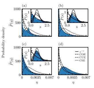
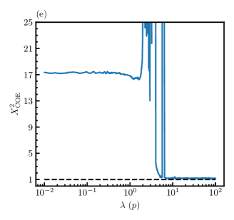
The kicked top is one of the best-studied models, both in classical and quantum chaos, and is extensively used to demonstrate the connection between the two [113]. Here, we use quantum kicked tops of different symmetries to provide concrete examples of both the dynamical signatures of quantum chaos and the RMT properties discussed above. Quantum kicked-kicked tops of COE and CSE symmetries are given by the Floquet operator:
| (38) |
with
| (39) | |||
| (40) |
for COE, and
| (41) | |||
| (42) |
for CSE. The kicked top with CUE symmetry is obtained by the following Floquet operator:
| (43) |
For further details on these different quantum kicked-top symmetries, see the Refs [113, 56]. The parameters used for the numerical simulation below are: (COE) , (regular) & (chaotic), and , (CUE) , , , and , and (CSE) , , , , and . In the dynamical simulations, we use the COE symmetry with the initial state , and the perturbation fidelity decay signature is obtained by comparing the quantum kicked tops with kick strengths of and .
A.4.1 Static Signatures
Here, we discuss the procedures and nuances involved in calculating the level-spacing and the eigenvector statistics, illustrating them with quantum kicked-top examples.
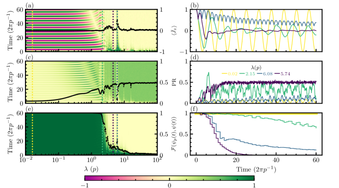
Level-spacing statistics
In this paper, for the quantum kicked-top models here and the DQS models in the main text, we mostly calculate the level spacing statistics using the eigenphases of a unitary evolution operator , which are unique up to a difference for any integer . This means that, for a given unitary operator, there are infinitely many corresponding Hermitian operators with the same eigenvectors but different eigenvalue spectrums. This is an important limitation for level-spacing statistics. Moreover, regardless of the non-uniqueness, an unfolding procedure is required to remove system-dependent secular variations and make the level spacings of any eigen-phase/value spectrum comparable with Wigner-Dyson distributions. Full details on level spacing statistics and unfolding are already found in many references [53, 54, 114, 115], but the main calculation steps are:
-
•
Sort the eigen-values/phases and group them into symmetry-reduced sub-spaces.
-
•
Unfolding: renormalise the local density of states by a smooth function to have both global and local unit-average level spacings.
-
•
Calculate the level spacings for each symmetry-reduced sub-spaces and create histograms with these spacings.
-
•
Normalise the area under the histogram to 1 and compare it with Wigner-Dyson distributions.
We can also superimpose the statistics of all these sub-spaces to have better resolution in the histogram plots [113].
Insets in Fig. 8 show the level spacing statistics for (a) COE with regular, (b) COE with quantum chaotic, and (c) CUE with quantum chaotic parameters. For regular parameters, it closely follows the Poisson statistics, and chaotic cases follow the corresponding Wigner-Dyson distribution of each class. They are super-imposed histograms of two sub-spaces. CUE and COE unitaries given above are symmetric under a rotation around the y-axis, and two symmetry reduced sub-spaces are determined by even and odd eigenstates of [113].
Obviously, it is also possible to define a goodness-of-fit test statistic to quantify agreement with Wigner-Dyson level-spacing statistics, but since the eigenvector statistics already provide a necessary and sufficient condition for quantum chaotic dynamics (and are generally easier to calculate), we have not included any such calculations here.
Eigenvector statistics
Once an appropriate basis is chosen, calculation of eigenvectors is almost trivial using the prescription in Appendix A.3. The only subtlety in this procedure arises when the system has degeneracies. For example, when comparing eigenvector statistics against the CSE distribution, which exhibits Kramers degeneracies, you need to take the degeneracies into account by summing the amplitudes for the degenerate levels, and this procedure decreases the degrees of freedom by half. The derivation of the CSE distribution in Eq. (35) already takes these into account [56]. Note that it can be any two levels, so you do not have to identify the exact degeneracies [56]. For the other symmetries, the same procedure also applies for degenerate cases, and the distributions in Eqs (33–34) need to be used with the decreased degree of freedom, e.g., , see Heisenberg model DQS with . In degenerate cases, however, the diagonalization routine may give random results even in non-random cases, due to the linear freedom in choosing the degenerate eigenvectors [98], and one needs to ensure that results are not affected by the diagonalization routine.
Figures 8 (a–d) show the eigenvector statistics, respectively, for (a) COE with regular, and (b) COE, (c) CUE and (d) CSE with quantum chaotic parameters. We observe close agreements (disagreement) between the eigenvector statistics of quantum chaotic (regular) systems and the corresponding RMT distributions. We also quantify the agreement/disagreement by calculating the goodness-of-fit test statistic between the eigenvector statistics of quantum kicked top of COE symmetry and the corresponding RMT distribution as a function of kick strength. In Fig. 8 (e), shows three main regions: (i) regular dynamics for , (ii) a transition region for with mixed-phase space and stable regions, and (iii) the quantum chaotic region for . Next, we demonstrate the same transition and regions in dynamical signatures of quantum chaos.
A.4.2 Dynamical Signatures
Here, we demonstrate onset of quantum chaos in the dynamics of a quantum kicked top with COE symmetry as a function of kick strength. Figure 9 shows the time evolutions of (a) (normalised) expectation value , (b) participation ratio (PR), and (c) fidelity under perturbation. Beyond the critical kicking strength , the system starts to show quantum chaotic characteristics: (i) destruction of quasiperiodicity in expectation values, (ii) high delocalisation, (iii) rapid perturbation fidelity decay. Figures 9 (d–f) show time traces for various kick-strengths, and we clearly see the quantum chaotic (and regular) dynamics as well as the revival of regular dynamics within the stable region marked (and plotted) by blue, which is also identified in the analysis of eigenvector statistics.
Appendix B Other Signatures of Quantum Chaos
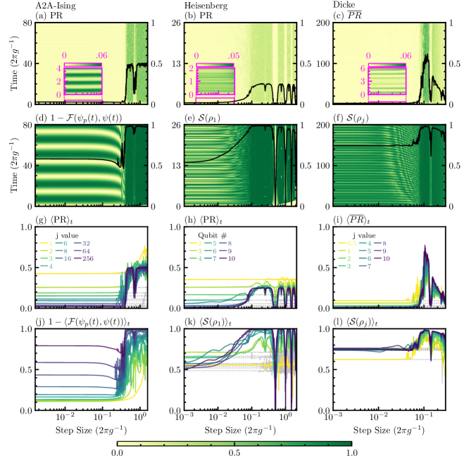
In the main text, we used our observation of the clear qualitative destruction of quasiperiodicity to illustrate a transition to quantum chaotic dynamics as a function of step size. In this section, we conduct a more quantitative study of this transition using a number of dynamical signatures underpinned by the connection of quantum chaos to ergodic dynamics and thermalisation.
For a closed system with a pure initial state, a concept of thermalisation can only be achieved in a context where the ergodic hypothesis holds, namely for dynamics where the time and state-space averages match for any macroscopic observable. Quantum chaotic dynamics provide a natural mechanism to achieve this condition for quantum systems [54, 102, 103, 22]. Specifically, quantum chaos drives a thermalisation-like process by dynamically delocalising the system state to span a large portion of the Hilbert space. This process, which relates to the simple intuitive description of quantum chaotic dynamics as being exponentially sensitive to perturbations in system parameters, is reflected for composite quantum systems in an increase of sub-system entropy. To study these concepts, in the following sections, we discuss example measures quantifying de-localisation, perturbation sensitivity, and entropy.
Delocalisation
We first quantify the delocalisation of the time-evolved state in a given basis by means of the participation ratio (PR) [45, 46],
| (44) |
where is the dimension of the Hilbert space. Quantum chaotic dynamics acts to create delocalisation, but to see this effect, it is important to choose an initial state and basis such that the state is initially localised. In this definition, the normalisation factor ensures the PR lies between for a fully localised state and 1 for a fully delocalised state. In the Dicke model, the cavity is infinite dimensional, and the choice of is non-trivial. We here choose a finite (labelled ) and justify this choice in Sec. 4.2.
Figures 10 (a–c) & (g–i) show that the temporal evolutions of PRs for A2A-Ising, Heisenberg, and Dicke models, and their time averages, are all clearly separated into localised and delocalised regions at the same step sizes as other quantities in Fig. 3. In A2A-Ising and Heisenberg Trotterisations, the PR beyond the threshold saturates to maximum values that can be well understood in terms of RMT symmetries and the choice of initial state. The maximum PR value is related to the RMT class and the choice of basis , and it is limited to 0.5, as observed in Fig. 10 (a) for A2A-Ising DQS, for further details see the discussions in Ref. [46]. While the PR for the Heisenberg DQS saturates to (Fig. 10 (b)) for this particular initial state, the results in Appendix D.3 studying initial-state dependence for the Heisenberg model show that the PR saturates to 0.5 for most states.
The maximum PR values in the Dicke model are more difficult to interpret due to our observation that the finite spin-ensemble dimension appears to limit how far the state can delocalise in the infinite dimensional cavity space (discussed further in later sections). Nevertheless, it is clear that the system shows larger delocalisation beyond the threshold. We also observe that the follows the same decaying trend beyond the stable region seen in the photon number. Our numerical analyses do not provide an explanation for this behaviour, which we leave as an open question.
Fidelity decay
Sensitivity to small perturbations in system parameters is one of the most widely appreciated characteristics of quantum chaotic dynamics. This concept can be quantified via a variety of related signatures such as fidelity decay, Loschmidt amplitude and echo, and out-of-time order correlators (OTOCs) [67, 52, 116, 117, 76], which are also useful in other contexts like quantum phase transitions and systems with broken time-reversal symmetries [116, 117, 76]. However, a drawback is that such signatures are reliable only if the perturbation itself does not show RMT distributions in its eigenvector statistics [52].
Here, we look at the perturbation fidelity, defined as the overlap
| (45) |
between two states evolved from the same initial state under a unitary and a perturbed unitary [67]. In the case of quantum kicked top pertaining to the A2A-Ising model, we identify a reliable perturbation by applying to the Trotter step unitary (see also Appendix A.4). Figures 10 (d) & (j) shows that the fidelity decay, or rather, here, the complementary perturbation error (infidelity under perturbation) , displays a regular oscillating signature before the threshold, and a characteristic exponential decay after, providing further strong evidence of the digitisation-induced transition to quantum chaotic dynamics. This trend is observed also for very small perturbations, with the perturbation strength only affecting the oscillation and decay rates in the two regimes.
Sub-system Entropy
For the Heisenberg and Dicke models, we illustrate an alternative signature of quantum chaotic dynamics that does not require perturbative comparisons, namely the increase of entanglement between subsystems, as characterised by the sub-system entropy [118, 119, 120, 22].
Here, we consider a normalised von Neumann entropy,
| (46) |
where is the reduced state of sub-system with dimension . The normalisation factor rescales the usual entropy to be in for any sub-system dimension, simplifying comparisons between different systems. This signature can be measured experimentally via tomography of the sub-system state, but importantly does not require access to the full system state [22]. Figures 10 (e–f) & (k–l) show that sub-system entropies jump to much larger values beyond the digitisation threshold for both the Heisenberg model (qubit 1) and the Dicke model (the spin- sub-system). In Sec. 4.2, we show that this entropy approaches the maximum value asymptotically with system size.
The observations of delocalisation, fidelity decay, and increased sub-system entropies beyond the threshold provide strong evidence for the quantum chaotic dynamics, complementing the more quantitatively rigorous evidence using random matrix theory statistics provided in Sec. 4.3. Combined with the observation that time averages of expectation values saturate to the relevant Hilbert-space means for each model and observable, for in A2A-Ising (Fig. 3 (a)), for Heisenberg (Fig. 3 (b)), and cavity and qubit parity in the Dicke model (not shown), they also provide evidence for the idea that the digitisation-induced quantum chaos is driving ergodicity beyond the threshold.
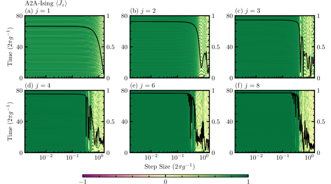
Appendix C Ising Model
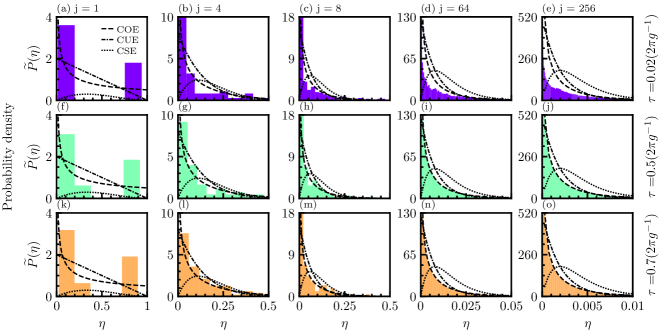
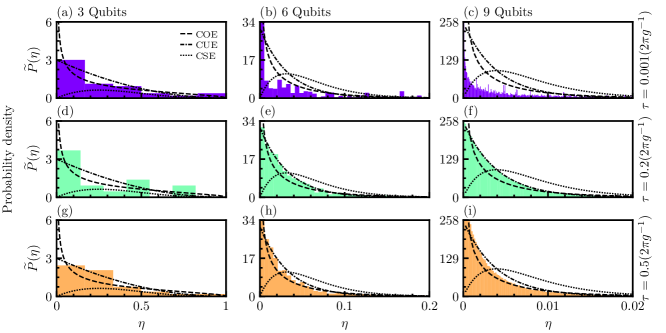
C.1 Dynamics in Small Systems
Here, we show dynamics for the magnetisation for small values in A2A-Ising Trotterisation. Figure 11 shows that the threshold gets sharper as the dynamics start to show quantum chaotic characteristics, namely the destruction of quasiperiodicity, beyond the threshold. Even though the approximate threshold position is still clear for any system size in Fig. 11, it is a smooth transition when the system is still quasiperiodic beyond the threshold, and it gets sharper only when the quasiperiodicity is destroyed for sufficiently large values. In Fig. 11, we observe that the sudden threshold and signatures of quantum chaotic dynamics start to appear for , and this observation is consistent with our analysis in the main text, which shows for .
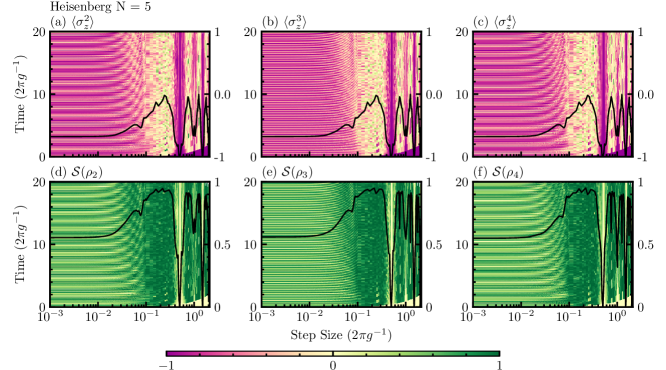
C.2 Eigenvector Statistics
In the main text of the paper, we show eigenvector statistics histograms for and calculate for the other system sizes. Here, to illustrate how system size affects the histograms themselves, we provide example histograms for several values and three step sizes, which are chosen from regular (before the threshold), quantum chaotic (after the threshold), and stable revival regions. Figure 12 shows the eigenvector statistics for different values on each column and different step sizes on each row: (top to bottom) before the threshold (), quantum chaotic (), and stable revival (seen only in large system sizes) () regions, respectively. The smallest system size, in Fig. 12 (a), does not have enough components to produce meaningful statistics, and the visual comparisons in Figs 12 (b–c) do not provide very clear conclusions. The goodness-of-fit test statistic, on the other hand, provides consistent conclusions in terms of successfully identifying the disagreement/agreement of eigenvector statistics with RMT distributions. For the large system sizes, the regular and chaotic regions are clearly distinguishable in the eigenvector statistics, shown respectively for (d) and (e) in Figs 12 (d–e). However, the stable regions () are visually indistinguishable from the quantum chaotic case, and, once again, proves useful and identifies these weak islands (see main text).
C.3 Stable Regions
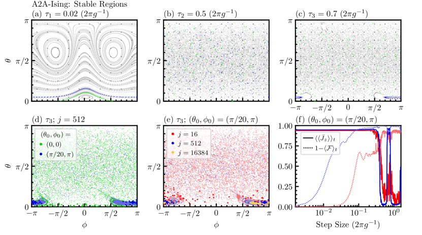
In the A2A-Ising model, we demonstrate that the revivals in stability observed beyond the threshold can be connected with the familiar notion of stable islands in an otherwise chaotic classical phase space. Here, the semiclassical limit is identical to the thermodynamic limit [53]. In particular, the commutators of rescaled spin components , etc., vanish in the limit , so that , , and become effectively classical variables. The stroboscopic classical evolution on the unit sphere of normalized vectors results from taking the semiclassical limit of the Heisenberg-picture evolution equations . Using the shorthand and defining , the evolution equations read [46]
| (47) |
The dynamics are best visualised by parametrising the classical phase space through spherical coordinates and via . This leads to the phase-space portraits shown in Fig. 15 for (a) , (b) , and (c) . Grey dots in the figure correspond to 200 iterations of the stroboscopic map Eq. (47) for 100 uniformly distributed initial states; The initial states for the trajectories shown in green and blue are given by, respectively, and . In a quantum system with finite as shown in Fig. 1, the above values of correspond to regular dynamics below the threshold, chaotic dynamics beyond the threshold, and the revival of regular dynamics in a stable region. For the classical phase space at the corresponding a stable region in the quantum domain (Fig. 15(c)), we also observe the re-appearance of a stable island, despite the phase space having already crossed over to be completely chaotic beyond the theshold (Fig. 15(b)). The initial state described by the green dots, , is chosen in Figs 15(a–c) to match the initial state chosen for the dynamical DQS simulations in Fig. 1. By contrast, the blue dots in Figs 15(a–c) show the trajectories for an initial state with , which lies on the stable island for Trotter steps within the stable region. Even at the classical level, the regular dynamics for the stable island in Fig. 15(c) are clearly different from the dynamics in Fig. 15(a), which are closer to the target dynamics; This accounts for the relatively poor revival of simulation fidelity in the stable region, as observed in the main text (see also Fig. 15(f)). However, while the classical component is relatively insensitive to the differences between these trajectories, we still see initial-state effects. Figure 15(d) shows the classical trajectories for a distribution of initial states selected according to spin coherent states with for the above states, and . The finite size of the spin coherent state leads to a finite overlap with both stable island and chaotic regions in classical phase space, but this becomes less pronounced with increasing spin as shown in Fig. 15(e), for phase space trajectories corresponding to , and with . Simulations of the Trotterised A2A-Ising dynamics for the first two of these spin sizes ( and ) are shown in Fig. 15(f). The revival becomes more marked with increasing spin size for the initial state , even while the simulation fidelity remains relatively low.
The quantum-classical correspondence principle suggests the following explanation for the changes observed in the local observable in Fig. 15(f) around : Trotter errors are inevitably large for trajectories corresponding to chaotic dynamics that is ergodic within the entire classical phase space (as for a completely mixed state). Trajectories within the stable islands of classical phase space follow regular dynamics that is generally restricted to a more localised region, and which therefore exhibits a different overlap with the target dynamics, from that corresponding to an underlying classically chaotic trajectory. Hence the re-emergence of stable islands in the A2A-Ising’s classical phase space accompanies the revival of stability in the stable regions of the Trotterised quantum model, for initial states which overlap with the stable islands. But note again with caution that, as in the case of the Trotterised Heisenberg model, the observed revivals of stability do not typically correspond to any revival in the quality of simulation with an underlying target model.
Appendix D Heisenberg Model
D.1 Eigenvector Statistics
In the main text, we present only the analysis for the Heisenberg Trotterisations. Therefore here, Fig. 13 explicitly shows the eigenvector statistics histogram plots for 3, 6, and 9 qubits Heisenberg Trotterisations on each column and different step sizes on each row. The step sizes shown in the columns of Fig. 13 are, respectively from top-to-bottom, from before the threshold (), quantum chaotic (), and stable revival () regions. For the case of 9 qubits, the histogram plots clearly agree/disagree with the RMT distributions in all three cases as seen in Figs 13 (c,f,i). The eigenvector statistics of the 6 qubits case show visually convincing agreement (and disagreement) in the quantum chaotic (and regular) regime as shown in Fig. 13 (b) (and (e)). However, for the 6 qubits case, the distinction between the stable revival and quantum chaotic regimes is not as clear as it is for 9 qubits. Finally, for the smallest system size in Fig. 13, none of the histogram plots provides any clear conclusion. By contrast, in each case, the analysis used in the main text of the paper provides quantitative measures of these visual comparisons, and successfully identifies all these regimes providing conclusive and consistent results.
As a final note, this Trotterisation has degeneracies. Therefore, the eigenvector statistics in Fig. 13 are calculated using the procedure discussed in Appendix A.4.1. Consequently, the number of independent components is reduced by half, so the theoretical lines in Fig. 13 are for for the case of qubits. These degeneracies are removed when the longitudinal field term is replaced with the transverse field term. Then, the regular procedure can be followed, and we observed a good agreement with RMT distributions of the full dimension . In both cases, the results regarding the threshold and the onset of quantum chaos beyond it are qualitatively the same both in the eigenvector statistics and the dynamical signatures (not shown, data available).
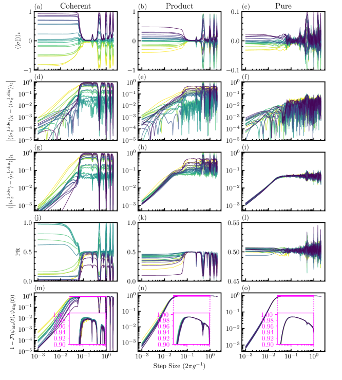
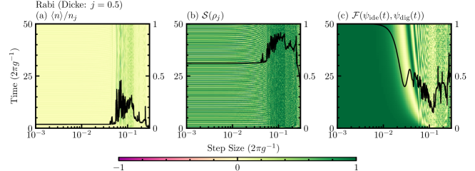
D.2 Dynamics of the Other Qubits in the Chain
In the main text of the paper, we use the first qubit of the chain to demonstrate the dynamics of the expectation values and subsystem entropies in the Trotterisation of the Heisenberg model, and we argue that the onset of quantum chaos and the threshold position is independent of this particular choice by using eigenvector statistics of the Trotter step unitary as well as sub-system independent dynamical quantities such as PR and simulation fidelity. Here, we provide the dynamics of the expectation values and the subsystem entropies for the second, third and fourth qubits of the chain of 5 qubits. Figs 14 (a–c) (and (d–f)) show the dynamics of expectation values (and subsystem entropies), respectively, for (a) (and (d)) second, (b) (and (e)) third, and (c) (and (f)) fourth qubit. We clearly observe the same threshold and same behaviours observed for the first qubit.
D.3 Effect of Initial State on the Threshold
Trotterisation of the Heisenberg model show certain initial-state-dependent effects in the main text of the paper. Here, we analyse the dynamics of the 9-qubit Trotterised Heisenberg model for various initial states (of 3 types) and provide results for expectation values, PR values, and the Trotter errors. The results show that the initial state does affect the size of the Trotterisation errors before the threshold and we note that the threshold might not seem as sudden for the states with larger errors. Still, the breakdown of digitisation occurs at a distinct threshold largely independent of the initial state.
We sample 20 initial states uniformly at random from each spin-coherent, product, and pure state types, where the spin-coherent state
| (48) |
is just a subset of product states , which is a subset of pure states. Figure 16 shows various averaged quantities calculated from the digital simulations for . Even for initially highly delocalised states (and the pure state samples), there is a noticeable difference at the same threshold position, and we observe the same threshold in each quantity and initial state.
Appendix E Dicke Model
E.1 Threshold in Rabi model
Here, we include the full dynamics of photon number, subsystem entropy, and simulation fidelity in the Rabi model (i.e., Dicke model with ). Figure 17 shows that the Rabi model already shows a strong threshold in all these quantities, and we observe signatures of quantum chaotic dynamics beyond the threshold. We see that the quasiperiodic dynamics of the (normalised) photon number is destroyed beyond the threshold (Figure 17 (a)), and that the subsystem entropy of the spin component is considerably larger than the pre-threshold value (Fig. 17 (b)), which is maximised for sufficiently large spin components in the Dicke model (Fig. 10 (l)). Finally, the threshold in simulation fidelity, shown in Fig. 17 (c), again appears as the secondary transition from (quasiperiodic) oscillatory-in-time to decaying behaviour. Despite the threshold and signatures of quantum chaotic dynamics beyond it, we do not find an agreement with RMT in the eigenvector statistics of the Rabi model. Instead, the Dicke model, similar to the other models, shows agreement with RMT predictions only for sufficiently large system sizes (in this case, a sufficiently large spin component), but it also shows certain cavity dimension truncation dependencies discussed in Appendix E.3. We leave further analyses of the threshold in the Rabi model, and why it appears at the smallest sizes, as an open question for future research.
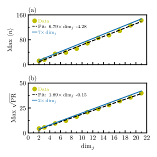
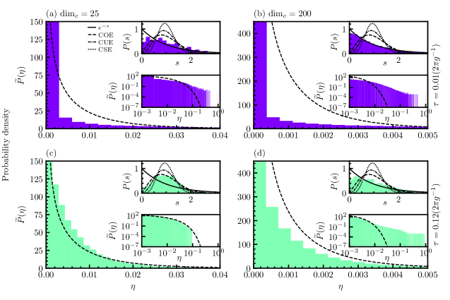
E.2 Normalisation of the Photon Number and the Participation Ratio
In this section, we present numerical data supporting our choice of normalisation coefficients and for, respectively, the photon numbers and PRs in the Dicke model. Figures 18 (a–b) show that the maximum of (a) the photon numbers and (b) the values of the quantum chaotic regions are linear in . We use and for the normalisations of the photon number and participation ratio, respectively, and the blue lines in Figs 18 (a–b) show these values. The constant coefficients 7 and 2 are determined numerically. The dynamical signatures are independent of the cavity truncation dimension , provided that is large enough for the simulation to support all the components of the time evolving state. Therefore, these observations (together with the maximised subsystem entropy of the spin component) suggest that the quantum chaos in this model is driven by the spin- component. The eigenvector statistics analyses, in the next section, support this intuition as they show agreement with the RMT distributions only when the cavity truncation is .
E.3 Eigenvector Statistics and the Effect of Truncated Cavity Dimension
In the numerical analyses of the Dicke DQS, the finite truncation of the cavity dimension poses a non-trivial problem. Here, we provide detailed numerical analysis of the truncation dependency in the eigenvector (and also eigenvalue) statistics of the Trotter step unitary of the Dicke model. We first present the histogram plots for the eigenvalue and eigenvector statistics for the case for different step sizes and cavity dimensions. Then, we carry out the analysis for the eigenvector statistics for various values and as a function of various parameters. Our numerical analysis gives us some intuitive physical insight and suggests that the spin component of the system drives the quantum chaotic dynamics beyond the threshold. We report our numerical findings to support and explain our choice for cavity truncation in the main text of the paper, and to provide initial motivation for further research. This is a subtle problem which merits further investigation of how to apply these statistics for truncated dimensions in unbounded systems, as well as a more rigorous understanding and explanation of these numerical results.
E.3.1 Level-spacing and Eigenvector Statistics
In this section, we provide the eigenvector statistics histograms for the Dicke DQS to show the cavity dimension truncation dependency, and we also employ an additional static signature of quantum chaos as a supporting tool, namely the level-spacing (or eigen-phase/value) statistics (discussed in Appendix A.2). Here, the level-spacing statistics are calculated for each parity subspace of the Dicke system (, see Appendix A.4.1), and the figures in this section show the super-imposed statistics of these subspaces. Additionally, the eigenvector statistics of the Dicke DQS are obtained using the degenerate system procedure (discussed in Appendix A.4.1). Therefore we use the RMT distributions with half the total size of the truncated space .
Figure 19, for the Dicke DQS, shows the level-spacing statistics in the upper-right insets, and the eigenvector statistics in the main figures with its tail in the lower-right insets. In Figs 19 (a–b), we use the step size (i.e. before the threshold), and we show that neither the eigenvector nor the eigenphase statistics have an agreement with RMT distributions, as expected. The eigenphase statistics are actually Poisson distributed for this step size, which is a signature of regular dynamics according to the Berry-Tabor conjecture [88]. For the step size (beyond the threshold) and the cavity dimension , both the eigenvector and eigenphase statistics show agreement with RMT distributions, shown in Fig. 19 (c). However, once exceeds a certain value (that increases with , as shown in the next section), agreement with RMT is lost in both of these cases, shown for in Fig. 19 (d) where the level-spacing statistics are actually closest to a Poisson distribution.
Aside from the dependency, both eigenvector and level-spacing statistics simultaneously agree/disagree with RMT beyond/before the threshold, and they show the same behaviour in various other system parameter regimes (not shown). Indeed, this even holds for examples the regime where the ideal Dicke model itself is known to be quantum chaotic [85, 86], where we still observe a distinct threshold, beyond which the PR values and sub-system entropies are larger for the digitised system than the ideal system. Since our focus in this paper is the digitisation-induced onset of quantum chaos, detailed analysis of this case is beyond the scope of this paper, but we provide some illustrative data in Appendix E.4.
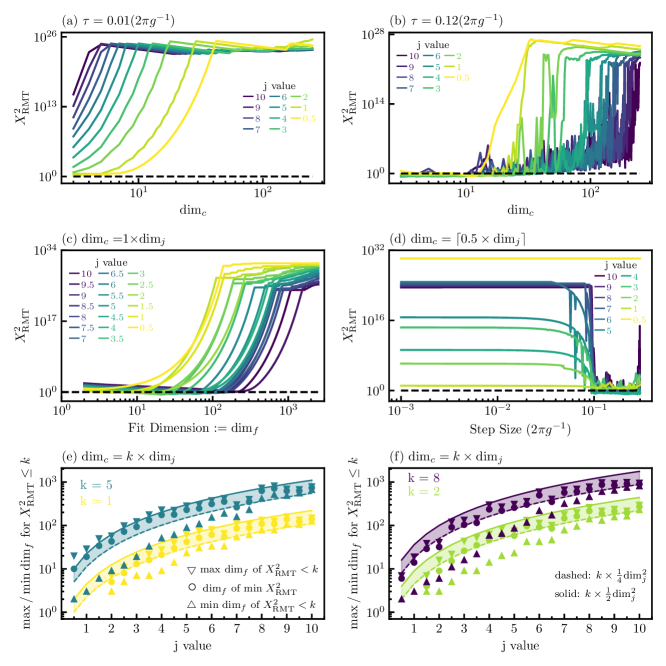
E.3.2 Goodness-of-fit Analyses
In this section, we analyse the dependency of eigenvector statistics on the truncation value of cavity dimension via the goodness-of-fit test statistic. In the previous section, we presented the eigenvector (and eigenphase) statistics histograms of the Trotter step unitary of the Dicke model with for two different step sizes and two cavity truncation values. We compared these statistics with RMT distributions of dimension (i.e. half the total size of the truncated space). Here, we calculate as a function of various parameters: namely cavity truncation , Trotter step size , spin size , and fit dimension . Here, we use the fit dimension to explore the effective system dimension. That is, with the other parameters fixed (including the cavity dimension), we instead sweep the dimension variable of the RMT distributions: we calculate by comparing the numerical eigenvector histograms to RMT distributions with dimension instead of .
The main observation from the results below is that the maximum cavity truncation dimension to obtain is . Together with the behaviours of the dynamical quantities (discussed in the main text and Appendix E.2), these results suggest that quantum chaotic dynamics in the Dicke DQS is mainly driven by the spin component. This is consistent with a simple intuition that the non-commutations in the Dicke DQS result from single qubit rotations that affect only the collective spin component. We nevertheless note the importance of developing a more theoretically rigorous understanding of these numerical results as an open question for further studies.
Cavity truncation
First, we analyse as a function of for two step sizes before () and after () the threshold and various values. In this case, the fit dimension is equal to the total dimension of the truncated system, i.e. . Figure 20 (a) shows that the eigenvector statistics before the threshold do not show agreement with RMT for any value of or . For the quantum chaotic region beyond the threshold, however, we observe that up to a maximum (that increases with increasing ) as shown in Fig. 20 (b), and quickly diverges to larger values beyond these truncations.
Fit dimension
Having observed agreement with RMT for in Fig. 20 (b), we now fix the cavity dimension to and calculate while varying the fit dimension for various values. The data in Figure 20 (c) confirm that is observed only for : specifically, we observe that stays below 1 when is between a minimum () and a maximum . In Fig. 20 (e), we plot the minimum and maximum values with upper and lower (yellow) triangles, respectively. The at which achieves its minimum is shown in yellow circles. These values appear to converge towards each other as the value increases, and stay mainly between and . Accounting for the additional factor in due to the degeneracies in the system (as discussed in Appendix A.4.1), this means that the maximum after which starts to quickly increase is equal to the , which is the cavity dimension we set.
and
Next, we analyse these max and min values for larger cavity truncations. We already know from Fig. 20 (b) that does not reach below 1 for cavity truncations that are much larger than , but they are fit against the full system dimension while we here use the fit dimension as a free parameter. In this case, we observed that the qualitative shape of curves similar to Fig. 20 (c) (not shown) stays the same provided that is an integer multiple of and that the curves shift upwards in as the cavity truncation increases. Therefore, again does not go below 1 for these large cavity truncations, but it does become smaller than the integer multiplicative factor . Figs 20 (e–f) show that and at which the reaches below are multiples of the above dimension, respectively and , and they again converge towards each other for larger values and stay approximately between these two values.
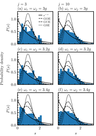
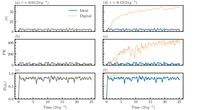
Step size
These results, though we leave it as an open question to find a rigorous explanation, show that the maximum truncation dimension that gives close agreement (i.e., ) with RMT is , which is also the value we used in the main text to analyse RMT correspondence as a function of step size. In the above results, the minimum cavity truncation that gives close agreement is observed to be . For comparison, here we plot for , as function of step size and for various system sizes (Fig. 20 (d)). It is qualitatively the same as the main text and shows the same threshold, showing that within this small range for , the results for the Dicke model do not depend sensitively on .
E.4 Quantum Chaos in Dicke model
In order to focus on digitisation-induced quantum chaos, we focus exclusively on regular parameters of the Dicke Hamiltonian in the main text of the paper. Here, we discuss how we choose these parameters, and also provide example results for the Trotterisation of the Dicke Hamiltonian with quantum chaotic parameters.
In two papers [86, 85], the Dicke model is shown be quantum chaotic for the coupling strengths around the critical coupling of the super-radiant phase transition (it becomes regular, if is either too much smaller or larger than ). For these regimes, Refs [86, 85] show that the level spacing statistics of the Dicke Hamiltonian follow Wigner-Dyson statistics. They support these observations by obtaining a classical correspondence using Holstein-Primakoff transformations, together with certain approximations, and showing that the classical limit is chaotic for the parameters that give Wigner-Dyson statistics in the quantum case.
E.4.1 Choice of the Parameters for the Main Text of the Paper
Here, we choose the Dicke model parameters used in the main text of the paper, by calculating the nearest-neighbour level-spacing statistics of the Dicke Hamiltonian for two values, and we find a parameter regime where it does not follow the Wigner-Dyson distribution. To do this, we need to find a combination of spin and cavity frequencies that are far enough from the superradiant phase transition point of the Dicke Hamiltonian. We can move far into either the superradiant or normal phase regime, and here we use the latter. Specifically, we gradually increase the product of the frequencies (which increases the critical coupling of the superradiant phase transition) until we stop observing Wigner-Dyson statistics. Using resonant spin and cavity frequencies, Fig. 21 shows this analysis for and , and we find that the level statistics fairly obviously do not agree with Wigner-Dyson statistics at both and by the time we have . Thus, any combination of spin and cavity frequencies that satisfy should be far enough from the quantum chaotic regime (which appears only for coupling frequencies near the super-radiant phase transition critical coupling).
E.4.2 Trotterisation of the Dicke Model with Quantum Chaotic Parameters
Our goal in this paper is to analyse digitisation-induced quantum chaos, therefore we use regular parameters of the Dicke model in the main text. We also, however, observed (not shown in detail) that the threshold behaviour is qualitatively the same for both regular and quantum chaotic parameters. It is not in the scope of this paper to provide detailed results for the threshold in the quantum chaotic regime of the Dicke model, but, here, we provide some example results (two different step sizes) for the Dicke model with quantum chaotic parameters ( and ). We show that the digitised dynamics closely follow the target dynamics for the small step size, and, for the large step size, it produces noticeably larger photon numbers, PR values, and sub-system entropies than the ideal Dicke evolution.
In Fig. 22, we compare the ideal and Trotterised dynamics for two step sizes, before and after the threshold, and observe that the Trotterised dynamics beyond the threshold show stronger signatures of quantum chaos than ideal dynamics. Figures 22 (a–c) show that ideal (blue) and Trotterised (orange) dynamics produce the same results before the threshold for (a) expectation, (b) PR, and (c) sub-system entropy of the spin component . We then compare the ideal dynamics with the Trotterised evolution beyond the threshold in Figs 22 (d–f), and we observe that the Trotterised dynamics produce stronger dynamical signatures of chaos, namely: (i) the destruction of quasiperiodicity in expectation values is much more prominent, (ii) PR for DQS is an order of magnitude greater than ideal, and (iii) entropy is maximised in DQS and larger than the ideal.
References
- [1] I. M. Georgescu, S. Ashhab, and Franco Nori. “Quantum simulation”. Rev. Mod. Phys. 86, 153–185 (2014). url: https://doi.org/10.1103/RevModPhys.86.153.
- [2] Christian Gross and Immanuel Bloch. “Quantum simulations with ultracold atoms in optical lattices”. Science 357, 995–1001 (2017). url: https://doi.org/10.1126/science.aal3837.
- [3] Hannes Bernien, Sylvain Schwartz, Alexander Keesling, Harry Levine, Ahmed Omran, Hannes Pichler, Soonwon Choi, Alexander S. Zibrov, Manuel Endres, Markus Greiner, Vladan Vuletić, and Mikhail D. Lukin. “Probing many-body dynamics on a 51-atom quantum simulator”. Nature 551, 579–584 (2017). url: https://doi.org/10.1038/nature24622.
- [4] J. Zhang, G. Pagano, P. W. Hess, A. Kyprianidis, P. Becker, H. Kaplan, A. V. Gorshkov, Z. X. Gong, and C. Monroe. “Observation of a many-body dynamical phase transition with a 53-qubit quantum simulator”. Nature 551, 601–604 (2017). url: https://doi.org/10.1038/nature24654.
- [5] Sepehr Ebadi, Tout T. Wang, Harry Levine, Alexander Keesling, Giulia Semeghini, Ahmed Omran, Dolev Bluvstein, Rhine Samajdar, Hannes Pichler, Wen Wei Ho, Soonwon Choi, Subir Sachdev, Markus Greiner, Vladan Vuletić, and Mikhail D. Lukin. “Quantum phases of matter on a 256-atom programmable quantum simulator”. Nature 595, 227–232 (2021). url: https://doi.org/10.1038/s41586-021-03582-4.
- [6] Pascal Scholl, Michael Schuler, Hannah J. Williams, Alexander A. Eberharter, Daniel Barredo, Kai-Niklas Schymik, Vincent Lienhard, Louis-Paul Henry, Thomas C. Lang, Thierry Lahaye, Andreas M. Läuchli, and Antoine Browaeys. “Quantum simulation of 2D antiferromagnets with hundreds of rydberg atoms”. Nature 595, 233–238 (2021). url: https://doi.org/10.1038/s41586-021-03585-1.
- [7] Bing Yang, Hui Sun, Robert Ott, Han-Yi Wang, Torsten V Zache, Jad C Halimeh, Zhen-Sheng Yuan, Philipp Hauke, and Jian-Wei Pan. “Observation of gauge invariance in a 71-site Bose–Hubbard quantum simulator”. Nature 587, 392–396 (2020). url: https://doi.org/10.1038/s41586-020-2910-8.
- [8] Alexander Mil, Torsten V Zache, Apoorva Hegde, Andy Xia, Rohit P Bhatt, Markus K Oberthaler, Philipp Hauke, Jürgen Berges, and Fred Jendrzejewski. “A scalable realization of local U(1) gauge invariance in cold atomic mixtures”. Science 367, 1128–1130 (2020). url: https://doi.org/10.1126/science.aaz5312.
- [9] Mari Carmen Bañuls, Rainer Blatt, Jacopo Catani, Alessio Celi, Juan Ignacio Cirac, Marcello Dalmonte, Leonardo Fallani, Karl Jansen, Maciej Lewenstein, Simone Montangero, Christine A. Muschik, Benni Reznik, Enrique Rico, Luca Tagliacozza, Karel Van Acoleyen, Frank Verstraete, Uwe-Jens Wiese, Matthew Wingate, Jakub Zakrzewski, and Peter Zoller. “Simulating lattice gauge theories within quantum technologies”. The European physical journal D 74, 1–42 (2020). url: https://doi.org/10.1140/epjd/e2020-100571-8.
- [10] Seth Lloyd. “Universal quantum simulators”. Science 273, 1073–1078 (1996). url: https://doi.org/10.1126/science.273.5278.1073.
- [11] Alán Aspuru-Guzik, Anthony D. Dutoi, Peter J. Love, and Martin Head-Gordon. “Simulated quantum computation of molecular energies”. Science 309, 1704–1707 (2005). url: https://doi.org/10.1126/science.1113479.
- [12] P. J. J. O’Malley, R. Babbush, I. D. Kivlichan, J. Romero, J. R. McClean, R. Barends, J. Kelly, P. Roushan, A. Tranter, N. Ding, B. Campbell, Y. Chen, Z. Chen, B. Chiaro, A. Dunsworth, A. G. Fowler, E. Jeffrey, E. Lucero, A. Megrant, J. Y. Mutus, M. Neeley, C. Neill, C. Quintana, D. Sank, A. Vainsencher, J. Wenner, T. C. White, P. V. Coveney, P. J. Love, H. Neven, A. Aspuru-Guzik, and J. M. Martinis. “Scalable quantum simulation of molecular energies”. Phys. Rev. X 6, 031007 (2016). url: https://doi.org/10.1103/PhysRevX.6.031007.
- [13] Abhinav Kandala, Antonio Mezzacapo, Kristan Temme, Maika Takita, Markus Brink, Jerry M. Chow, and Jay M. Gambetta. “Hardware-efficient variational quantum eigensolver for small molecules and quantum magnets”. Nature 549, 242–246 (2017). url: https://doi.org/10.1038/nature23879.
- [14] Google AI Quantum and collaborators. “Hartree-Fock on a superconducting qubit quantum computer”. Science 369, 1084–1089 (2020). url: https://doi.org/10.1126/science.abb9811.
- [15] A Mezzacapo, U Las Heras, J S Pedernales, L DiCarlo, E Solano, and L Lamata. “Digital Quantum Rabi and Dicke models in superconducting circuits”. Scientific Reports 4, 7482 (2014). url: https://doi.org/10.1038/srep07482.
- [16] N K Langford, R Sagastizabal, M Kounalakis, C Dickel, A Bruno, F Luthi, D J Thoen, A Endo, and L DiCarlo. “Experimentally simulating the dynamics of quantum light and matter at deep-strong coupling”. Nature Communications 8, 1715 (2017). url: https://doi.org/10.1038/s41467-017-01061-x.
- [17] Lucas Lamata. “Digital-analog quantum simulation of generalized Dicke models with superconducting circuits”. Scientific Reports 7, 43768 (2017). url: https://doi.org/10.1038/srep43768.
- [18] B. P. Lanyon, C. Hempel, D. Nigg, M. Müller, R. Gerritsma, F. Zähringer, P. Schindler, J. T. Barreiro, M. Rambach, G. Kirchmair, M. Hennrich, P. Zoller, R. Blatt, and C. F. Roos. “Universal digital quantum simulation with trapped ions”. Science 334, 57–61 (2011). url: https://doi.org/10.1126/science.1208001.
- [19] U. Las Heras, A. Mezzacapo, L. Lamata, S. Filipp, A. Wallraff, and E. Solano. “Digital quantum simulation of spin systems in superconducting circuits”. Phys. Rev. Lett. 112, 200501 (2014). url: https://doi.org/10.1103/PhysRevLett.112.200501.
- [20] Y. Salathé, M. Mondal, M. Oppliger, J. Heinsoo, P. Kurpiers, A. Potočnik, A. Mezzacapo, U. Las Heras, L. Lamata, E. Solano, S. Filipp, and A. Wallraff. “Digital quantum simulation of spin models with circuit quantum electrodynamics”. Phys. Rev. X 5, 021027 (2015). url: https://doi.org/10.1103/PhysRevX.5.021027.
- [21] Rami Barends, L Lamata, Julian Kelly, L García-Álvarez, Austin G Fowler, A Megrant, Evan Jeffrey, Ted C White, Daniel Sank, Josh Y Mutus, et al. “Digital quantum simulation of fermionic models with a superconducting circuit”. Nature communications 6, 1–7 (2015). url: https://doi.org/10.1038/ncomms8654.
- [22] C. Neill, P. Roushan, M. Fang, Y. Chen, M. Kolodrubetz, Z. Chen, A. Megrant, R. Barends, B. Campbell, B. Chiaro, A. Dunsworth, E. Jeffrey, J. Kelly, J. Mutus, P. J. J. O’Malley, C. Quintana, D. Sank, A. Vainsencher, J. Wenner, T. C. White, A. Polkovnikov, and J. M. Martinis. “Ergodic dynamics and thermalization in an isolated quantum system”. Nature Physics 12, 1037 (2016). url: https://doi.org/10.1038/nphys3830.
- [23] Esteban A. Martinez, Christine A. Muschik, Philipp Schindler, Daniel Nigg, Alexander Erhard, Markus Heyl, Philipp Hauke, Marcello Dalmonte, Thomas Monz, Peter Zoller, and Rainer Blatt. “Real-time dynamics of lattice gauge theories with a few-qubit quantum computer”. Nature 534, 516–519 (2016). url: https://doi.org/10.1038/nature18318.
- [24] John Preskill. “Quantum Computing in the NISQ era and beyond”. Quantum 2, 79 (2018). url: https://doi.org/10.22331/q-2018-08-06-79.
- [25] H. F. Trotter. “On the product of semi-groups of operators”. Proceedings of the American Mathematical Society 10, 545–551 (1959). url: https://doi.org/10.2307/2033649.
- [26] Masuo Suzuki. “Generalized Trotter’s formula and systematic approximations of exponential operators and inner derivations with applications to many-body problems”. Communications in Mathematical Physics 51, 183–190 (1976). url: https://doi.org/10.1007/BF01609348.
- [27] Masuo Suzuki. “Decomposition formulas of exponential operators and Lie exponentials with some applications to quantum mechanics and statistical physics”. Journal of Mathematical Physics 26, 601–612 (1985). url: https://doi.org/10.1063/1.526596.
- [28] Masuo Suzuki. “Fractal decomposition of exponential operators with applications to many-body theories and Monte Carlo simulations”. Physics Letters A 146, 319–323 (1990). url: https://doi.org/10.1016/0375-9601(90)90962-N.
- [29] Masuo Suzuki. “General theory of fractal path integrals with applications to many-body theories and statistical physics”. Journal of Mathematical Physics 32, 400–407 (1991). url: https://doi.org/10.1063/1.529425.
- [30] Andrew M. Childs and Nathan Wiebe. “Hamiltonian simulation using linear combinations of unitary operations”. Quantum Info. Comput. 12, 901–924 (2012). url: https://doi.org/10.26421/QIC12.11-12.
- [31] Dominic W. Berry, Andrew M. Childs, Richard Cleve, Robin Kothari, and Rolando D. Somma. “Simulating Hamiltonian dynamics with a truncated Taylor series”. Phys. Rev. Lett. 114, 090502 (2015). url: https://doi.org/10.1103/PhysRevLett.114.090502.
- [32] Guang Hao Low and Isaac L. Chuang. “Optimal Hamiltonian simulation by quantum signal processing”. Phys. Rev. Lett. 118, 010501 (2017). url: https://doi.org/10.1103/PhysRevLett.118.010501.
- [33] Guang Hao Low and Isaac L. Chuang. “Hamiltonian Simulation by Qubitization”. Quantum 3, 163 (2019). url: https://doi.org/10.22331/q-2019-07-12-163.
- [34] Andrew M. Childs, Dmitri Maslov, Yunseong Nam, Neil J. Ross, and Yuan Su. “Toward the first quantum simulation with quantum speedup”. Proceedings of the National Academy of Sciences 115, 9456–9461 (2018). url: https://doi.org/10.1073/pnas.1801723115.
- [35] Andrew M. Childs, Yuan Su, Minh C. Tran, Nathan Wiebe, and Shuchen Zhu. “Theory of Trotter error with commutator scaling”. Phys. Rev. X 11, 011020 (2021). url: https://doi.org/10.1103/PhysRevX.11.011020.
- [36] Dominic W. Berry, Graeme Ahokas, Richard Cleve, and Barry C. Sanders. “Efficient quantum algorithms for simulating sparse Hamiltonians”. Communications in Mathematical Physics 270, 359–371 (2007). url: https://doi.org/10.1007/s00220-006-0150-x.
- [37] M. B. Hastings, D. Wecker, B. Bauer, and M. Troyer. “Improving quantum algorithms for quantum chemistry”. Quantum Info. Comput.Page 1–21 (2015). url: https://doi.org/10.48550/arXiv.1403.1539.
- [38] Dave Wecker, Bela Bauer, Bryan K. Clark, Matthew B. Hastings, and Matthias Troyer. “Gate-count estimates for performing quantum chemistry on small quantum computers”. Phys. Rev. A 90, 022305 (2014). url: https://doi.org/10.1103/PhysRevA.90.022305.
- [39] Sadegh Raeisi, Nathan Wiebe, and Barry C Sanders. “Quantum-circuit design for efficient simulations of many-body quantum dynamics”. New Journal of Physics 14, 103017 (2012). url: https://doi.org/10.1088%2F1367-2630%2F14%2F10%2F103017.
- [40] Earl Campbell. “Shorter gate sequences for quantum computing by mixing unitaries”. Phys. Rev. A 95, 042306 (2017). url: https://doi.org/10.1103/PhysRevA.95.042306.
- [41] Earl Campbell. “Random compiler for fast Hamiltonian simulation”. Phys. Rev. Lett. 123, 070503 (2019). url: https://doi.org/10.1103/PhysRevLett.123.070503.
- [42] Andrew M. Childs, Aaron Ostrander, and Yuan Su. “Faster quantum simulation by randomization”. Quantum 3, 182 (2019). url: https://doi.org/10.22331/q-2019-09-02-182.
- [43] David Poulin, M. B. Hastings, Dave Wecker, Nathan Wiebe, Andrew C. Doherty, and Matthias Troyer. “The Trotter step size required for accurate quantum simulation of quantum chemistry”. Quantum Info. Comput.Page 361–384 (2015). url: https://doi.org/10.48550/arXiv.1406.4920.
- [44] Ryan Babbush, Jarrod McClean, Dave Wecker, Alán Aspuru-Guzik, and Nathan Wiebe. “Chemical basis of Trotter-Suzuki errors in quantum chemistry simulation”. Phys. Rev. A 91, 022311 (2015). url: https://doi.org/10.1103/PhysRevA.91.022311.
- [45] Markus Heyl, Philipp Hauke, and Peter Zoller. “Quantum localization bounds Trotter errors in digital quantum simulation”. Science Advances 5, aau8342 (2019). url: https://doi.org/10.1126/sciadv.aau8342.
- [46] Lukas M. Sieberer, Tobias Olsacher, Andreas Elben, Markus Heyl, Philipp Hauke, Fritz Haake, and Peter Zoller. “Digital quantum simulation, Trotter errors, and quantum chaos of the kicked top”. npj Quantum Information 5, 78 (2019). url: https://doi.org/10.1038/s41534-019-0192-5.
- [47] Sergio Boixo, Sergei V. Isakov, Vadim N. Smelyanskiy, Ryan Babbush, Nan Ding, Zhang Jiang, Michael J. Bremner, John M. Martinis, and Hartmut Neven. “Characterizing quantum supremacy in near-term devices”. Nature Physics 14, 595–600 (2018). url: https://doi.org/10.1038/s41567-018-0124-x.
- [48] Frank Arute, Kunal Arya, Ryan Babbush, Dave Bacon, Joseph C. Bardin, Rami Barends, Rupak Biswas, Sergio Boixo, Fernando G. S. L. Brandao, David A. Buell, Brian Burkett, Yu Chen, Zijun Chen, Ben Chiaro, Roberto Collins, William Courtney, Andrew Dunsworth, Edward Farhi, Brooks Foxen, Austin Fowler, Craig Gidney, Marissa Giustina, Rob Graff, Keith Guerin, Steve Habegger, Matthew P. Harrigan, Michael J. Hartmann, Alan Ho, Markus Hoffmann, Trent Huang, Travis S. Humble, Sergei V. Isakov, Evan Jeffrey, Zhang Jiang, Dvir Kafri, Kostyantyn Kechedzhi, Julian Kelly, Paul V. Klimov, Sergey Knysh, Alexander Korotkov, Fedor Kostritsa, David Landhuis, Mike Lindmark, Erik Lucero, Dmitry Lyakh, Salvatore Mandrà, Jarrod R. McClean, Matthew McEwen, Anthony Megrant, Xiao Mi, Kristel Michielsen, Masoud Mohseni, Josh Mutus, Ofer Naaman, Matthew Neeley, Charles Neill, Murphy Yuezhen Niu, Eric Ostby, Andre Petukhov, John C. Platt, Chris Quintana, Eleanor G. Rieffel, Pedram Roushan, Nicholas C. Rubin, Daniel Sank, Kevin J. Satzinger, Vadim Smelyanskiy, Kevin J. Sung, Matthew D. Trevithick, Amit Vainsencher, Benjamin Villalonga, Theodore White, Z. Jamie Yao, Ping Yeh, Adam Zalcman, Hartmut Neven, and John M. Martinis. “Quantum supremacy using a programmable superconducting processor”. Nature 574, 505–510 (2019). url: https://doi.org/10.1038/s41586-019-1666-5.
- [49] Yulin Wu, Wan-Su Bao, Sirui Cao, Fusheng Chen, Ming-Cheng Chen, Xiawei Chen, Tung-Hsun Chung, Hui Deng, Yajie Du, Daojin Fan, Ming Gong, Cheng Guo, Chu Guo, Shaojun Guo, Lianchen Han, Linyin Hong, He-Liang Huang, Yong-Heng Huo, Liping Li, Na Li, Shaowei Li, Yuan Li, Futian Liang, Chun Lin, Jin Lin, Haoran Qian, Dan Qiao, Hao Rong, Hong Su, Lihua Sun, Liangyuan Wang, Shiyu Wang, Dachao Wu, Yu Xu, Kai Yan, Weifeng Yang, Yang Yang, Yangsen Ye, Jianghan Yin, Chong Ying, Jiale Yu, Chen Zha, Cha Zhang, Haibin Zhang, Kaili Zhang, Yiming Zhang, Han Zhao, Youwei Zhao, Liang Zhou, Qingling Zhu, Chao-Yang Lu, Cheng-Zhi Peng, Xiaobo Zhu, and Jian-Wei Pan. “Strong quantum computational advantage using a superconducting quantum processor”. Phys. Rev. Lett. 127, 180501 (2021). url: https://doi.org/10.1103/PhysRevLett.127.180501.
- [50] Qingling Zhu, Sirui Cao, Fusheng Chen, Ming-Cheng Chen, Xiawei Chen, Tung-Hsun Chung, Hui Deng, Yajie Du, Daojin Fan, Ming Gong, Cheng Guo, Chu Guo, Shaojun Guo, Lianchen Han, Linyin Hong, He-Liang Huang, Yong-Heng Huo, Liping Li, Na Li, Shaowei Li, Yuan Li, Futian Liang, Chun Lin, Jin Lin, Haoran Qian, Dan Qiao, Hao Rong, Hong Su, Lihua Sun, Liangyuan Wang, Shiyu Wang, Dachao Wu, Yulin Wu, Yu Xu, Kai Yan, Weifeng Yang, Yang Yang, Yangsen Ye, Jianghan Yin, Chong Ying, Jiale Yu, Chen Zha, Cha Zhang, Haibin Zhang, Kaili Zhang, Yiming Zhang, Han Zhao, Youwei Zhao, Liang Zhou, Chao-Yang Lu, Cheng-Zhi Peng, Xiaobo Zhu, and Jian-Wei Pan. “Quantum computational advantage via 60-qubit 24-cycle random circuit sampling”. Science Bulletin 67, 240–245 (2022). url: https://doi.org/10.48550/arXiv.2109.03494.
- [51] Lorenzo Leone, Salvatore F. E. Oliviero, You Zhou, and Alioscia Hamma. “Quantum Chaos is Quantum”. Quantum 5, 453 (2021). url: https://doi.org/10.22331/q-2021-05-04-453.
- [52] Joseph Emerson, Yaakov S. Weinstein, Seth Lloyd, and D. G. Cory. “Fidelity decay as an efficient indicator of quantum chaos”. Phys. Rev. Lett. 89, 284102 (2002). url: https://doi.org/10.1103/PhysRevLett.89.284102.
- [53] Fritz Haake, Sven Gnutzmann, and Marek Kuś. “Quantum signatures of chaos”. Springer. (2018). 4 edition. url: https://doi.org/10.1007/978-3-642-05428-0.
- [54] Luca D’Alessio, Yariv Kafri, Anatoli Polkovnikov, and Marcos Rigol. “From quantum chaos and eigenstate thermalization to statistical mechanics and thermodynamics”. Advances in Physics 65, 239–362 (2016). url: https://doi.org/10.1080/00018732.2016.1198134.
- [55] F.M. Izrailev. “Chaotic stucture of eigenfunctions in systems with maximal quantum chaos”. Physics Letters A 125, 250–252 (1987). url: https://doi.org/10.1016/0375-9601(87)90203-9.
- [56] M Kus, J Mostowski, and F Haake. “Universality of eigenvector statistics of kicked tops of different symmetries”. Journal of Physics A: Mathematical and General 21, L1073–L1077 (1988). url: https://doi.org/10.1088/0305-4470/21/22/006.
- [57] Neil Dowling and Kavan Modi. “Quantum chaos=volume-law spatiotemporal entanglement” (2022). url: https://doi.org/10.48550/arXiv.2210.14926.
- [58] Dmitry A. Abanin, Wojciech De Roeck, and Francois Huveneers. “Exponentially slow heating in periodically driven many-body systems”. Phys. Rev. Lett. 115, 256803 (2015). url: https://doi.org/10.1103/PhysRevLett.115.256803.
- [59] Takashi Mori, Tomotaka Kuwahara, and Keiji Saito. “Rigorous bound on energy absorption and generic relaxation in periodically driven quantum systems”. Phys. Rev. Lett. 116, 120401 (2016). url: https://doi.org/10.1103/PhysRevLett.116.120401.
- [60] Tomotaka Kuwahara, Takashi Mori, and Keiji Saito. “Floquet–Magnus theory and generic transient dynamics in periodically driven many-body quantum systems”. Annals of Physics 367, 96–124 (2016). url: https://doi.org/10.1016/j.aop.2016.01.012.
- [61] Dmitry A. Abanin, Wojciech De Roeck, Wen Wei Ho, and Francois Huveneers. “Effective Hamiltonians, prethermalization, and slow energy absorption in periodically driven many-body systems”. Phys. Rev. B 95, 014112 (2017). url: https://doi.org/10.1103/PhysRevB.95.014112.
- [62] Fernando Casas. “Sufficient conditions for the convergence of the Magnus expansion”. Journal of Physics A: Mathematical and Theoretical 40, 15001–15017 (2007). url: https://doi.org/10.1088/1751-8113/40/50/006.
- [63] Per Christian Moan and Jitse Niesen. “Convergence of the Magnus series”. Foundations of Computational Mathematics 8, 291–301 (2008). url: https://doi.org/10.1007/s10208-007-9010-0.
- [64] S. Blanes, F. Casas, J.A. Oteo, and J. Ros. “The Magnus expansion and some of its applications”. Physics Reports 470, 151–238 (2009). url: https://doi.org/10.1016/j.physrep.2008.11.001.
- [65] Takashi Ishii, Tomotaka Kuwahara, Takashi Mori, and Naomichi Hatano. “Heating in integrable time-periodic systems”. Phys. Rev. Lett. 120, 220602 (2018). url: https://doi.org/10.1103/PhysRevLett.120.220602.
- [66] Karthik Chinni, Manuel H. Muñoz Arias, Ivan H. Deutsch, and Pablo M. Poggi. “Trotter errors from dynamical structural instabilities of floquet maps in quantum simulation”. PRX Quantum 3, 010351 (2022). url: https://doi.org/10.1103/PRXQuantum.3.010351.
- [67] Asher Peres. “Stability of quantum motion in chaotic and regular systems”. Phys. Rev. A 30, 1610–1615 (1984). url: https://doi.org/10.1103/PhysRevA.30.1610.
- [68] Wolfgang Nolting and Anupuru Ramakanth. “Quantum theory of magnetism”. Springer-Verlag Berlin Heidelberg. (2009). 1 edition. url: https://doi.org/10.1007/978-3-540-85416-6.
- [69] I. I. Rabi. “On the process of space quantization”. Phys. Rev. 49, 324–328 (1936). url: https://doi.org/10.1103/PhysRev.49.324.
- [70] R. H. Dicke. “Coherence in spontaneous radiation processes”. Phys. Rev. 93, 99–110 (1954). url: https://doi.org/10.1103/PhysRev.93.99.
- [71] E. T. Jaynes and F. W. Cummings. “Comparison of quantum and semiclassical radiation theories with application to the beam maser”. Proceedings of the IEEE 51, 89–109 (1963). url: https://doi.org/10.1109/PROC.1963.1664.
- [72] Michael Tavis and Frederick W. Cummings. “Exact solution for an -molecule–radiation-field Hamiltonian”. Phys. Rev. 170, 379–384 (1968). url: https://doi.org/10.1103/PhysRev.170.379.
- [73] P. Forn-Díaz, L. Lamata, E. Rico, J. Kono, and E. Solano. “Ultrastrong coupling regimes of light-matter interaction”. Rev. Mod. Phys. 91, 025005 (2019). url: https://doi.org/10.1103/RevModPhys.91.025005.
- [74] Wojciech H. Zurek, Uwe Dorner, and Peter Zoller. “Dynamics of a quantum phase transition”. Phys. Rev. Lett. 95, 105701 (2005). url: https://doi.org/10.1103/PhysRevLett.95.105701.
- [75] M. Heyl, A. Polkovnikov, and S. Kehrein. “Dynamical quantum phase transitions in the transverse-field Ising model”. Phys. Rev. Lett. 110, 135704 (2013). url: https://doi.org/10.1103/PhysRevLett.110.135704.
- [76] Markus Heyl. “Dynamical quantum phase transitions: A brief survey”. EPL (Europhysics Letters) 125, 26001 (2019). url: https://doi.org/10.1209%2F0295-5075%2F125%2F26001.
- [77] Freeman J. Dyson, Elliott H. Lieb, and Barry Simon. “Phase transitions in the quantum Heisenberg model”. Phys. Rev. Lett. 37, 120–123 (1976). url: https://doi.org/10.1103/PhysRevLett.37.120.
- [78] Myung-Joong Hwang, Ricardo Puebla, and Martin B. Plenio. “Quantum phase transition and universal dynamics in the Rabi model”. Phys. Rev. Lett. 115, 180404 (2015). url: https://doi.org/10.1103/PhysRevLett.115.180404.
- [79] Andrew Lucas. “Ising formulations of many NP problems”. Frontiers in Physics 2, 5 (2014). url: https://doi.org/10.3389/fphy.2014.00005.
- [80] S Chaudhury, A Smith, B E Anderson, S Ghose, and P S Jessen. “Quantum signatures of chaos in a kicked top”. Nature 461, 768 (2009). url: https://doi.org/10.1038/nature08396.
- [81] Vincent Mourik, Serwan Asaad, Hannes Firgau, Jarryd J. Pla, Catherine Holmes, Gerard J. Milburn, Jeffrey C. McCallum, and Andrea Morello. “Exploring quantum chaos with a single nuclear spin”. Phys. Rev. E 98, 042206 (2018). url: https://doi.org/10.1103/PhysRevE.98.042206.
- [82] C. Monroe, W. C. Campbell, L.-M. Duan, Z.-X. Gong, A. V. Gorshkov, P. W. Hess, R. Islam, K. Kim, N. M. Linke, G. Pagano, P. Richerme, C. Senko, and N. Y. Yao. “Programmable quantum simulations of spin systems with trapped ions”. Rev. Mod. Phys. 93, 025001 (2021). url: https://doi.org/10.1103/RevModPhys.93.025001.
- [83] Juan P. Dehollain, Juha T. Muhonen, Kuan Y. Tan, Andre Saraiva, David N. Jamieson, Andrew S. Dzurak, and Andrea Morello. “Single-shot readout and relaxation of singlet and triplet states in exchange-coupled electron spins in silicon”. Phys. Rev. Lett. 112, 236801 (2014). url: https://doi.org/10.1103/PhysRevLett.112.236801.
- [84] M. Veldhorst, J. C. C. Hwang, C. H. Yang, A. W. Leenstra, B. de Ronde, J. P. Dehollain, J. T. Muhonen, F. E. Hudson, K. M. Itoh, A. Morello, and A. S. Dzurak. “An addressable quantum dot qubit with fault-tolerant control-fidelity”. Nature Nanotechnology 9, 981–985 (2014). url: https://doi.org/10.1038/nnano.2014.216.
- [85] Clive Emary and Tobias Brandes. “Quantum chaos triggered by precursors of a quantum phase transition: The Dicke model”. Phys. Rev. Lett. 90, 044101 (2003). url: https://doi.org/10.1103/PhysRevLett.90.044101.
- [86] Clive Emary and Tobias Brandes. “Chaos and the quantum phase transition in the Dicke model”. Phys. Rev. E 67, 066203 (2003). url: https://doi.org/10.1103/PhysRevE.67.066203.
- [87] O. Bohigas, M. J. Giannoni, and C. Schmit. “Characterization of chaotic quantum spectra and universality of level fluctuation laws”. Phys. Rev. Lett. 52, 1–4 (1984). url: https://doi.org/10.1103/PhysRevLett.52.1.
- [88] Michael Victor Berry, M. Tabor, and John Michael Ziman. “Level clustering in the regular spectrum”. Proceedings of the Royal Society of London. A. Mathematical and Physical Sciences 356, 375–394 (1977). url: https://doi.org/10.1098/rspa.1977.0140.
- [89] Pedram Roushan, Charles Neill, J Tangpanitanon, Victor M Bastidas, A Megrant, Rami Barends, Yu Chen, Z Chen, B Chiaro, A Dunsworth, A Fowler, B Foxen, M Giustina, E Jeffrey, J Kelly, E Lucero, J Mutus, M Neeley, C Quintana, D Sank, A Vainsencher, J Wenner, T White, H Neven, D G Angelakis, and J Martinis. “Spectroscopic signatures of localization with interacting photons in superconducting qubits”. Science 358, 1175–1179 (2017). url: https://doi.org/10.1126/science.aao1401.
- [90] Lata Kh Joshi, Andreas Elben, Amit Vikram, Benoît Vermersch, Victor Galitski, and Peter Zoller. “Probing many-body quantum chaos with quantum simulators”. Physical Review X 12, 011018 (2022). url: https://doi.org/10.1103/PhysRevX.12.011018.
- [91] Denis V Vasilyev, Andrey Grankin, Mikhail A Baranov, Lukas M Sieberer, and Peter Zoller. “Monitoring quantum simulators via quantum nondemolition couplings to atomic clock qubits”. PRX Quantum 1, 020302 (2020). url: https://doi.org/10.1103/PRXQuantum.1.020302.
- [92] Fritz Haake and Karol Życzkowski. “Random-matrix theory and eigenmodes of dynamical systems”. Phys. Rev. A 42, 1013–1016 (1990). url: https://doi.org/10.1103/PhysRevA.42.1013.
- [93] Freeman J. Dyson. “Statistical theory of the energy levels of complex systems. i”. Journal of Mathematical Physics 3, 140–156 (1962). url: https://doi.org/10.1063/1.1703773.
- [94] B. Georgeot and D. L. Shepelyansky. “Quantum chaos border for quantum computing”. Phys. Rev. E 62, 3504–3507 (2000). url: https://doi.org/10.1103/PhysRevE.62.3504.
- [95] B. Georgeot and D. L. Shepelyansky. “Emergence of quantum chaos in the quantum computer core and how to manage it”. Phys. Rev. E 62, 6366–6375 (2000). url: https://doi.org/10.1103/PhysRevE.62.6366.
- [96] P. G. Silvestrov, H. Schomerus, and C. W. J. Beenakker. “Limits to error correction in quantum chaos”. Phys. Rev. Lett. 86, 5192–5195 (2001). url: https://doi.org/10.1103/PhysRevLett.86.5192.
- [97] D. L. Shepelyansky. “Quantum chaos and quantum computers”. Physica Scripta T90, 112 (2001). url: https://doi.org/10.1238%2Fphysica.topical.090a00112.
- [98] Daniel Braun. “Quantum chaos and quantum algorithms”. Phys. Rev. A 65, 042317 (2002). url: https://doi.org/10.1103/PhysRevA.65.042317.
- [99] G. Benenti, G. Casati, S. Montangero, and D. L. Shepelyansky. “Statistical properties of eigenvalues for an operating quantum computer with static imperfections”. The European Physical Journal D - Atomic, Molecular, Optical and Plasma Physics 22, 285–293 (2003). url: https://doi.org/10.1140/epjd/e2002-00241-9.
- [100] K. A. Landsman, C. Figgatt, T. Schuster, N. M. Linke, B. Yoshida, N. Y. Yao, and C. Monroe. “Verified quantum information scrambling”. Nature 567, 61–65 (2019). url: https://doi.org/10.1038/s41586-019-0952-6.
- [101] Xiao Mi, Pedram Roushan, Chris Quintana, Salvatore Mandra, Jeffrey Marshall, Charles Neill, Frank Arute, Kunal Arya, Juan Atalaya, Ryan Babbush, Joseph C. Bardin, Rami Barends, Andreas Bengtsson, Sergio Boixo, Alexandre Bourassa, Michael Broughton, Bob B. Buckley, David A. Buell, Brian Burkett, Nicholas Bushnell, Zijun Chen, Benjamin Chiaro, Roberto Collins, William Courtney, Sean Demura, Alan R. Derk, Andrew Dunsworth, Daniel Eppens, Catherine Erickson, Edward Farhi, Austin G. Fowler, Brooks Foxen, Craig Gidney, Marissa Giustina, Jonathan A. Gross, Matthew P. Harrigan, Sean D. Harrington, Jeremy Hilton, Alan Ho, Sabrina Hong, Trent Huang, William J. Huggins, L. B. Ioffe, Sergei V. Isakov, Evan Jeffrey, Zhang Jiang, Cody Jones, Dvir Kafri, Julian Kelly, Seon Kim, Alexei Kitaev, Paul V. Klimov, Alexander N. Korotkov, Fedor Kostritsa, David Landhuis, Pavel Laptev, Erik Lucero, Orion Martin, Jarrod R. McClean, Trevor McCourt, Matt McEwen, Anthony Megrant, Kevin C. Miao, Masoud Mohseni, Wojciech Mruczkiewicz, Josh Mutus, Ofer Naaman, Matthew Neeley, Michael Newman, Murphy Yuezhen Niu, Thomas E. O’Brien, Alex Opremcak, Eric Ostby, Balint Pato, Andre Petukhov, Nicholas Redd, Nicholas C. Rubin, Daniel Sank, Kevin J. Satzinger, Vladimir Shvarts, Doug Strain, Marco Szalay, Matthew D. Trevithick, Benjamin Villalonga, Theodore White, Z. Jamie Yao, Ping Yeh, Adam Zalcman, Hartmut Neven, Igor Aleiner, Kostyantyn Kechedzhi, Vadim Smelyanskiy, and Yu Chen. “Information scrambling in quantum circuits”. Science 374, 1479–1483 (2021). url: https://doi.org/10.1126/science.abg5029.
- [102] J. M. Deutsch. “Quantum statistical mechanics in a closed system”. Phys. Rev. A 43, 2046–2049 (1991). url: https://doi.org/10.1103/PhysRevA.43.2046.
- [103] Mark Srednicki. “Chaos and quantum thermalization”. Phys. Rev. E 50, 888–901 (1994). url: https://doi.org/10.1103/PhysRevE.50.888.
- [104] Lukas J Fiderer and Daniel Braun. “Quantum metrology with quantum-chaotic sensors”. Nature Communications 9, 1351 (2018). url: https://doi.org/10.1038/s41467-018-03623-z.
- [105] Cahit Kargi, Fabio Henriques, Angsar Manatuly, Adrien Di Lonardo, Giorge Gemisis, Juan Pablo Dehollain, and Nathan K. Langford. “QuanGuru”. https://github.com/CirQuS-UTS/QuanGuru (2021).
- [106] Eugene P. Wigner. “Characteristic vectors of bordered matrices with infinite dimensions”. Annals of Mathematics 62, 548–564 (1955). url: https://doi.org/10.1007/978-3-662-02781-3_35.
- [107] E. B. Bogomolny, B. Georgeot, M.-J. Giannoni, and C. Schmit. “Chaotic billiards generated by arithmetic groups”. Phys. Rev. Lett. 69, 1477–1480 (1992). url: https://doi.org/10.1103/PhysRevLett.69.1477.
- [108] Hua Wu, Michel Vallières, Da Hsuan Feng, and Donald W. L. Sprung. “Gaussian-orthogonal-ensemble level statistics in a one-dimensional system”. Phys. Rev. A 42, 1027–1032 (1990). url: https://doi.org/10.1103/PhysRevA.42.1027.
- [109] G. Casati, B. V. Chirikov, and I. Guarneri. “Energy-level statistics of integrable quantum systems”. Phys. Rev. Lett. 54, 1350–1353 (1985). url: https://doi.org/10.1103/PhysRevLett.54.1350.
- [110] Mario Feingold and Asher Peres. “Distribution of matrix elements of chaotic systems”. Phys. Rev. A 34, 591–595 (1986). url: https://doi.org/10.1103/PhysRevA.34.591.
- [111] A. M. Mood, F. A. Graybill, and D. C. Boes. “Introduction to the theory of statistics”. McGraw-Hill. New York, NY, USA (1974). Third edition. url: https://doi.org/10.1017/S0020269X00004552.
- [112] Nicolas Regnault and Rahul Nandkishore. “Floquet thermalization: Symmetries and random matrix ensembles”. Phys. Rev. B 93, 104203 (2016). url: https://doi.org/10.1103/PhysRevB.93.104203.
- [113] F. Haake, M. Kuś, and R. Scharf. “Classical and quantum chaos for a kicked top”. Zeitschrift für Physik B Condensed Matter 65, 381–395 (1987). url: https://doi.org/10.1007/BF01303727.
- [114] Simon Sirca and Martin Horvat. “Computational methods for physicists: compendium for students”. Springer Science & Business Media. (2012). url: https://doi.org/10.1007/978-3-642-32478-9.
- [115] Wimberger Sandro. “Nonlinear dynamics and quantum chaos: An introduction”. SPRINGER. (2016). url: https://doi.org/10.1007/978-3-319-06343-0.
- [116] Thomas Gorin, Tomaz Prosen, Thomas H. Seligman, and Marko Znidaric. “Dynamics of Loschmidt echoes and fidelity decay”. Physics Reports 435, 33–15 (2006). url: https://doi.org/10.1016/j.physrep.2006.09.003.
- [117] Arseni Goussev, Rodolfo A. Jalabert, Horacio M. Pastawski, and Diego Wisniacki. “Loschmidt echo”. Scholarpedia 7, 11687 (2012). url: https://doi.org/10.4249/scholarpedia.11687.
- [118] K. Furuya, M. C. Nemes, and G. Q. Pellegrino. “Quantum dynamical manifestation of chaotic behavior in the process of entanglement”. Phys. Rev. Lett. 80, 5524–5527 (1998). url: https://doi.org/10.1103/PhysRevLett.80.5524.
- [119] Jayendra N. Bandyopadhyay and Arul Lakshminarayan. “Testing statistical bounds on entanglement using quantum chaos”. Phys. Rev. Lett. 89, 060402 (2002). url: https://doi.org/10.1103/PhysRevLett.89.060402.
- [120] Carlos Mejía-Monasterio, Guliano Benenti, Gabriel G. Carlo, and Giulio Casati. “Entanglement across a transition to quantum chaos”. Phys. Rev. A 71, 062324 (2005). url: https://doi.org/10.1103/PhysRevA.71.062324.
