RoMA: a Method for Neural Network Robustness Measurement and Assessment

Abstract

Neural network models have become the leading solution for a large variety of tasks, such as classification, natural language processing, and others. However, their reliability is heavily plagued by adversarial inputs: inputs generated by adding tiny perturbations to correctly-classified inputs, and for which the neural network produces erroneous results. In this paper, we present a new method called Robustness Measurement and Assessment (RoMA), which measures the robustness of a neural network model against such adversarial inputs. Specifically, RoMA determines the probability that a random input perturbation might cause misclassification. The method allows us to provide formal guarantees regarding the expected frequency of errors that a trained model will encounter after deployment. The type of robustness assessment afforded by RoMA is inspired by state-of-the-art certification practices, and could constitute an important step toward integrating neural networks in safety-critical systems.

1 Introduction

In the passing decade, deep neural networks (DNNs) have emerged as one of the most exciting developments in computer science, allowing computers to outperform humans in various classification tasks. However, a major issue with DNNs is the existence of adversarial inputs [11]: inputs that are very close (according to some metrics) to correctly-classified inputs, but which are misclassified themselves. It has been observed that many state-of-the-art DNNs are highly vulnerable to adversarial inputs [6].

As the impact of the AI revolution is becoming evident, regulatory agencies are starting to address the challenge of integrating DNNs into various automotive and aerospace systems — by forming workgroups to create the needed guidelines. Notable examples in the European Union include SAE G-34 and EUROCAE WG-114 [21, 26]; and the European Union Safety Agency (EASA), which is responsible for civil aviation safety, and which has published a road map for certifying AI-based systems [9]. These efforts, however, must overcome a significant gap: on one hand, the superior performance of DNNs makes it highly desirable to incorporate them into various systems, but on the other hand, the DNN’s intrinsic susceptibility to adversarial inputs could render them unsafe. This dilemma is particularly felt in safety-critical systems, such as automotive, aerospace and medical devices, where regulators and public opinion set a high bar for reliability.

In this work, we seek to begin bridging this gap, by devising a framework that could allow engineers to bound and mitigate the risk introduced by a trained DNN, effectively containing the phenomenon of adversarial inputs. Our approach is inspired by common practices of regulatory agencies, which often need to certify various systems with components that might fail due to an unexpected hazard. A widely used example is the certification of jet engines, which are known to occasionally fail. In order to mitigate this risk, manufacturers compute the engines’ mean time between failures (MTBF), and then use this value in performing a safety analysis that can eventually justify the safety of the jet engine system as a whole [17]. For example, federal agencies guide that the probability of an extremely improbable failure conditions event per operational hour should not exceed $10^{-9}$ [17]. To perform a similar process for DNN-based systems, we first need a technique for accurately bounding the likelihood of a failure to occur — e.g., for measuring the probability of encountering an adversarial input.

In this paper, we address the aforesaid crucial gap, by introducing a straightforward and scalable method for measuring the probability that a DNN classifier misclassifies inputs. The method, which we term Robustness Measurement and Assessment (RoMA), is inspired by modern certification concepts, and operates under the assumption that a DNN’s misclassification is due to some internal malfunction, caused by random input perturbations (as opposed to misclassifications triggered by an external cause, such as a malicious adversary). A random input perturbation can occur naturally as part of the system’s operation, e.g., due to scratches on a camera lens or communication disruptions. Under this assumption, RoMA can be used to measure the model’s robustness to randomly-produced adversarial inputs.

RoMA is a method for estimating rare events in a large population — in our case, adversarial inputs within a space of inputs that are generally classified correctly. When these rare events (adversarial inputs) are distributed normally within the input space, RoMA performs the following steps: it (i) samples a few hundred random input points; (ii) measures the “level of adversariality” of each such point; and (iii) uses the normal distribution function to evaluate the probability of encountering an adversarial input within the input space. Unfortunately, adversarial inputs are often not distributed normally. To overcome this difficulty, when RoMA detects this case it first applies a statistical power transformation, called Box-Cox [5], after which the distribution often becomes normal and can be analyzed. The Box-Cox transformation is a widespread method that does not pose any restrictions on the DNN in question (e.g., Lipschitz continuity, certain kinds of activation functions, or specific network topology). Further, the method does not require access to the network’s design or weights, and is thus applicable to large, black-box DNNs.

We implemented our method as a proof-of-concept tool, and evaluated it on a VGG16 network trained on the CIFAR10 data set. Using RoMA, we were able to show that, as expected, a higher number of epochs (a higher level of training) leads to a higher robustness score. Additionally, we used RoMA to measure how the model’s robustness score changes as the magnitude of allowed input perturbation is increased. Finally, using RoMA we found that the categorial robustness score of a DNN, which is the robustness score of inputs labeled as a particular category, varies significantly among the different categories.

To summarize, our main contributions are: (i) introducing RoMA, which is a new and scalable method for measuring the robustness of a DNN model, and which can be applied to black-box DNNs; (ii) using RoMA to measure the effect of additional training on the robustness of a DNN model; (iii) using RoMA to measure how a model’s robustness changes as the magnitude of input perturbation increases; and (iv) formally computing categorial robustness scores, and demonstrating that they can differ significantly between labels.

Related work. The topic of statistically evaluating a model’s adversarial robustness has been studied extensively. State-of-the-art approaches [14, 7] assume that the confidence scores assigned to perturbed images are normally distributed, and apply random sampling to measure robustness. However, as we later demonstrate, this assumption often does not hold. Other approaches [27, 25, 19] use a sampling method called importance sampling, where a few bad samples with large weights can drastically throw off the estimator. Further, these approaches typically assume that the network’s output is Lipschitz-continuous. Although RoMA is similar in spirit to these approaches, it requires no Lipschitz-continuity, does not assume a-priori that the adversarial input confidence scores are distributed normally, and provides rigorous robustness guarantees.

Other noticeable methods for measuring robustness include formal-verification based approaches [15, 16], which are exact but which afford very limited scalability; and approaches for computing an estimate bound on the probability that a classifier’s margin function exceeds a given value [28, 1, 8], which focus on worst-case behavior, and may consequently be inadequate for regulatory certification. In contrast, RoMA is a scalable method, which focuses on the more realistic, average case.

2 Background

Neural Networks. A neural network $N$ is a function $N:\mathbb{R}^{n}\rightarrow\mathbb{R}^{m}$, which maps a real-valued input vector $\vec{x}\in\mathbb{R}^{n}$ to a real-value output vector $\vec{y}\in\mathbb{R}^{m}$. For classification networks, which is our subject matter, $\vec{x}$ is classified as label $l$ if $y$’s $l$’th entry has the highest score; i.e., if $\operatorname*{arg\,max}(N(\vec{x}))=l$.

Local Adversarial Robustness. The local adversarial robustness of a DNN is a measure of how resilient that network is against adversarial perturbations to specific inputs. More formally [3]:

Definition 1

A DNN $N$ is $\epsilon$-locally-robust at input point $\vec{x_{0}}$ iff

$$\forall\vec{x}.\displaystyle||\vec{x}-\vec{x_{0}}||_{\infty}\leq\epsilon\Rightarrow\operatorname*{arg\,max}(N(\vec{x}))=\operatorname*{arg\,max}(N(\vec{x_{0}}))$$

Intuitively, Definition 1 states that for input vector $\vec{x}$, which is at a distance at most $\epsilon$ from a fixed input $\vec{x_{0}}$, the network function assigns to $\vec{x}$ the same label that it assigns to $\vec{x_{0}}$ (for simplicity, we use here the $L_{\infty}$ norm, but other metrics could also be used). When a network is not $\epsilon$-local-robust at point $\vec{x_{0}}$, there exists a point $\vec{x}$ that is at a distance of at most $\epsilon$ from $\vec{x_{0}}$, which is misclassified; this $\vec{x}$ is called an adversarial input. In this context, local refers to the fact that $\vec{x_{0}}$ is fixed.

Distinct Adversarial Robustness. Recall that the label assigned by a classification network is selected according to its greatest output value. The final layer in such networks is usually a softmax layer, and its outputs are commonly interpreted as confidence scores assigned to each of the possible labels. We use $c(\vec{x})$ to denote the highest confidence score, i.e. $c(\vec{x})=max(N(\vec{x}))$.

We are interested in an adversarial input $\vec{x}$ only if it is distinctly misclassified [17]; i.e., if $\vec{x}$’s assigned label receives a significantly higher score than that of the label assigned to $\vec{x_{0}}$. For example, if $\operatorname*{arg\,max}(N(\vec{x_{0}}))\neq\operatorname*{arg\,max}(N(\vec{x}))$, but $c(\vec{x})=20\%$, then $\vec{x}$ is not distinctly an adversarial input: while it is misclassified, the network assigns it an extremely low confidence score. Indeed, in a safety-critical setting, the system is expected to issue a warning to the operator when it has such low confidence in its classification [20]. In contrast, a case where $c(\vec{x})=80\%$ is much more distinct: here, the network gives an incorrect answer with high confidence, and no warning to the operator is expected. We refer to inputs that are misclassified with confidence greater than some threshold $\delta$ as distinctly adversarial inputs, and refine Definition 1 to only consider them, as follows:

Definition 2

A DNN $N$ is ($\epsilon,\delta$)-distinctly-locally-robust at input point $\vec{x_{0}}$, iff

$$\forall\vec{x}.\ \displaystyle||\vec{x}-\vec{x_{0}}||_{\infty}\leq\epsilon\Rightarrow\big{(}\operatorname*{arg\,max}(N(\vec{x}))=\operatorname*{arg\,max}(N(\vec{x_{0}}))\big{)}\vee(c(\vec{x})<\delta)$$

Intuitively, if the definition does not hold then there exists a (distinctly) adversarial input $\vec{x}$ that is at most $\epsilon$ away from $\vec{x_{0}}$, and which is assigned a label different than that of $\vec{x_{0}}$ with a confidence score that is at least $\delta$.

3 The Proposed Method

3.1 Probabilistic Robustness

Definitions 1 and 2 are geared for an external, malicious adversary: they are concerned with the existence of an adversarial input. Here, we take a different path, and follow common certification methodologies that deal with internal malfunctions of the system [10]. Specifically, we focus on “non-malicious adversaries” — i.e., we assume that perturbations occur naturally, and are not necessarily malicious. This is represented by assuming those perturbations are randomly drawn from some distribution. We argue that the non-malicious adversary setting is more realistic for widely-deployed systems in, e.g., aerospace, which are expected to operate at a large scale and over a prolonged period of time, and are more likely to encounter randomly-perturbed inputs than those crafted by a malicious adversary.

Targeting randomly generated adversarial inputs requires extending Definitions 1 and 2 into a probabilistic definition, as follows:

Definition 3

The $(\delta,\epsilon)$-probabilistic-local-robustness score of a DNN $N$ at input point $\vec{x_{0}}$, abbreviated $\text{plr}{}{}_{\delta,\epsilon}(N,\vec{x_{0}})$, is defined as:

$$\text{plr}{}{}_{\delta,\epsilon} (N,\vec{x_{0}})\triangleq P_{x:\lVert\vec{x}-\vec{x_{0}}\rVert_{\infty}\leq\epsilon}[(\operatorname*{arg\,max}(N(\vec{x}))=\operatorname*{arg\,max}(N(\vec{x_{0}}))\lor c(\vec{x})<\delta)]$$

Intuitively, the definition measures the probability that an input $\vec{x}$, drawn at random from the $\epsilon$-ball around $\vec{x_{0}}$, will either have the same label as $\vec{x_{0}}$ or, if it does not, will receive a confidence score lower than $\delta$ for its (incorrect) label.

A key point is that probabilistic robustness, as defined in Definition 3, is a scalar value: the closer this value is to 1, the less likely it is a random perturbation to $\vec{x_{0}}$ would produce a distinctly adversarial input. This is in contrast to Definitions 1 and 2, which are Boolean in nature. We also note that the probability value in Definition 3 can be computed with respect to values of $\vec{x}$ drawn according to any input distribution of interest. For simplicity, unless otherwise stated, we assume that $\vec{x}$ is drawn uniformly at random.

In practice, we propose to compute $\text{plr}{}{}_{\delta,\epsilon}(N,\vec{x})$ by first computing the probability that a randomly drawn $\vec{x}$ is a distinctly adversarial input, and then taking that probability’s complement. Unfortunately, directly bounding the probability of randomly encountering an adversarial input, e.g., with the Monte Carlo or Bernoulli methods [13], is not feasible due to the typical extreme sparsity of adversarial inputs, and the large number of samples required to achieve reasonable accuracy [27]. Thus, we require a different statistical approach to obtain this measure, using only a reasonable number of samples. We next propose such an approach.

3.2 Sampling Method and the Normal Distribution

Our approach is to measure the probability of randomly encountering an adversarial input, by examining a finite set of perturbed samples around $\vec{x_{0}}$. Each perturbation is selected through simple random sampling [24] (although other sampling methods can be used), while ensuring that the overall perturbation size does not exceed the given $\epsilon$. Next, each perturbed input $\vec{x}$ is passed through the DNN to obtain a vector of confidence scores for the possible output labels. From this vector, we extract the highest incorrect confidence (hic) score:

$$\text{hic}{}(\vec{x})=\max_{i\neq\operatorname*{arg\,max}(N(\vec{x_{0}}))}\{N(\vec{x})[i]\}$$

which is the highest confidence score assigned to an incorrect label, i.e., a label different from the one assigned to $\vec{x_{0}}$. Observe that input $\vec{x}$ is distinctly adversarial if and only if its hic score exceeds the $\delta$ threshold.

The main remaining question is how to extrapolate from the collected hic values a conclusion regarding the hic values in the general population. The normal distribution is a useful notion in this context: if the hic values are distributed normally (as determined by a statistical test), it is straightforward to obtain such a conclusion, even if adversarial inputs are scarce.

To illustrate this process, we trained a VGG16 DNN model (information about the trained model and the dataset appears in Section 4), and examined an arbitrary point $\vec{x_{0}}$, from its test set. We randomly generated 10,000 perturbed images around $\vec{x_{0}}$ with $\epsilon=0.04$, and ran them through the DNN. For each output vector obtained this way we collected the hic value, and then plotted these values as the blue histogram in Figure 1. The green curve represents the normal distribution. As the figure shows, the data is normally distributed; this claim is supported by running a “goodness-of-fit” test (explained later).

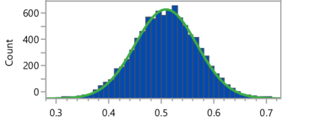
Figure 1: A histogram depicting the highest incorrect confidence (hic) scores assigned to each of 10,000 perturbed inputs. These scores are normally distributed.

Our goal is to compute the probability of a fresh, randomly-perturbed input to be distinctly misclassified, i.e. to be assigned a hic score that exceeds a given $\delta$, say $60\%$. For data distributed normally, as in this case, we begin by calculating the statistical standard score (Z-Score), which is the number of standard deviations by which the value of a raw score exceeds the mean value. Using the Z-score, we can compute the probability of the event using the Gaussian function. In our case, we get $\text{hic}{}(\vec{x})\sim\mathcal{N}(\mu=0.499,\Sigma=0.059^{2})$, where $\mu$ is the average score and $\Sigma$ is the variance. The Z-score is $\frac{\delta-\mu}{\sigma}=\frac{0.6-0.499}{0.059}=1.741$, where $\sigma$ is the standard deviation. Recall that our goal is to compute the plr score, which is the probability of the hic value not exceeding $\delta$; and so we obtain that:

$$\text{plr}{}{}_{0.6,0.04}(N,\vec{x_{0}}) =\text{NormalDistribution}{}(\text{Z-score})$$

$$=\text{NormalDistribution}{}(1.741)$$

$$=\frac{1}{\sqrt{2\pi}}\int_{-\infty}^{t=1.741}e^{\frac{-t^{2}}{2}}dt=0.9591$$

We thus arrive at a probabilistic local robustness score of $95.91\%$.

Because our data is obtained empirically, before we can apply the aforementioned approach we need a reliable way to determine whether the data is distributed normally. A goodness-of-fit test is a procedure for determining whether a set of $n$ samples can be considered as drawn from a specified distribution. A common goodness-of-fit test for the normal distribution is the Anderson-Darling test [2], which focuses on samples in the tails of the distribution [4]. In our evaluation, a distribution was considered normal only if the Anderson-Darling test returned a score value greater than $\alpha=0.15$, which is considered a high level of significance — guaranteeing that no major deviation from normality was found.

3.3 The Box-Cox Transformation

Unfortunately, most often the hic values are not normally distributed. For example, in our experiments we observed that only 1,282 out of the 10,000 images in the CIFAR10’s test set (fewer than 13%) demonstrated normally-distributed hic values. Figure 2 illustrates the abnormal distribution of hic values of perturbed inputs around one of the input points. In such cases, we cannot use the normal distribution function to estimate the probability of adversarial inputs in the population.

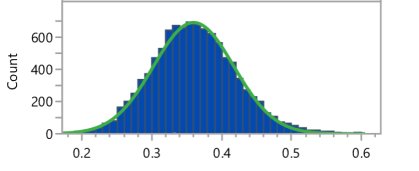
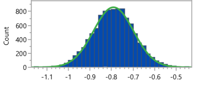
Figure 2: On the top: a histogram depicting the highest incorrect confidence (hic) scores of each of 10,000 perturbed inputs around one of the test points. These scores are not normally distributed. Beneath: the same scores after applying the Box-Cox power transformation, now normally distributed.

The strategy that we propose for handling abnormal distributions of data, like the one depicted in Figure 2, is to apply statistical transformations. Such transformations preserve key properties of the data, while producing a normally distributed measurement scale [12] — effectively converting the given distribution into a normal one. There are two main transformations used to normalize probability distributions: Box-Cox [5] and Yeo-Johnson [29]. Here, we focus on the Box-Cox power transformation, which is preferred for distributions of positive data values (as in our case). Box-Cox is a continuous, piecewise-linear power transform function, parameterized by a real-valued $\lambda$, defined as follows:

Definition 4

The Box-Cox_λ power transformation of input $x$ is:

$$\ BoxCox_{\lambda}(x)=\begin{cases}\frac{x^{\lambda}-1}{\lambda}&if\lambda\neq 0\\ \ln(x)&if\lambda=0\end{cases}$$

The selection of the $\lambda$ value is crucial for the successful normalization of the data. There are multiple automated methods for $\lambda$ selection, which go beyond our scope here [22]. For our implementation of the technique, we used the common SciPy Python package [23], which implements one of these automated methods.

Figure 2 depicts the distribution of the data from Figure 2, after applying the Box-Cox transformation, with an automatically calculated $\lambda=0.534$ value. As the figure shows, the data is now normally distributed: $\text{hic}{}(\vec{x})\sim\mathcal{N}(\mu=-0.79,\Sigma=0.092^{2})$. The normal distribution was confirmed with the Anderson-Darling test. Following the Box-Cox transformation, we can now calculate the Z-Score, which gives $3.71$, and the corresponding plr score, which turns out to be 99.98%.

3.4 The RoMA Certification Algorithm

Based on the previous sections, our method for computing plr scores is given as Algorithm 1. The inputs to the algorithm are: (i) $\delta$, the confidence threshold for a distinctly adversarial input; (ii) $\epsilon$, the maximum amplitude of perturbation that can be added to $\vec{x_{0}}$; (iii) $\vec{x_{0}}$, the input point whose plr score is being computed; (iv) $n$, the number of perturbed samples to generate around $\vec{x_{0}}$; (v) $N$, the neural network; and (vi) $\mathcal{D}$, the distribution from which perturbations are drawn. The algorithm starts by generating $n$ perturbed inputs around the provided $\vec{x_{0}}$, each drawn according to the provided distribution $\mathcal{D}$ and with a perturbation that does not exceed $\epsilon$ (lines 1–2); and then storing the hic score of each of these inputs in the hic array (line 3). Next, lines 5–10 confirm that the samples’ hic values distribute normally, applying the Box-Cox transformation if needed. Finally, on lines 11–13, the algorithm calculates the probability of randomly perturbing the input into a distinctly adversarial input using the properties of the normal distribution, and returns the computed $\text{plr}{}{}_{\delta,\epsilon}(N,\vec{x_{0}})$ score on line 14.

Algorithm 1 Compute Probabilistic Local Robustness($\delta,\epsilon,\vec{x_{0}},n,N,\mathcal{D}$)

1:  for $i:=1$ to $n$ do

2:     $\vec{x^{i}}$ = CreatePerturbedPoint($\vec{x_{0}},\epsilon,\mathcal{D}$)

3:     hic[i] $\leftarrow$ Predict($N,\vec{x^{i}}$)

4:  end for

5:  if Anderson-Darling(hic $\neq$ NORMAL) then

6:     hic $\leftarrow$ Box-Cox(hic)

7:     if Anderson-Darling(hic $\neq$ NORMAL) then

8:        Return “Fail”

9:     end if

10:  end if

11:  avg $\leftarrow$ Average(hic)

12:  std $\leftarrow$ StdDev(hic)

13:  z-score $\leftarrow$ Z-Score(avg,std,$BoxCox(\delta$))

14:  Return NormalDistribution(z-score)

Soundness and Completeness. Algorithm 1 depends on the distribution of $\text{hic}{}(\vec{x})$ being normal. If this is initially not so, the algorithm attempts to normalize it using the Box-Cox transformation. The Anderson-Darling goodness-of-fit test ensures that the algorithm does not treat an abnormal distribution as a normal one, and thus guarantees the soundness of the computed plr scores.

The algorithm’s completeness depends on its ability to always obtain a normal distribution. As our evaluation demonstrates, the Box-Cox transformation can indeed lead to a normal distribution very often. However, the transformation might fail in producing a normal distribution; this failure will be identified by the Anderson-Darling test, and our algorithm will stop with a failure notice in such cases. In that sense, Algorithm 1 is incomplete. In practice, failure notices by the algorithm can sometimes be circumvented — by increasing the sample size, or by evaluating the robustness of other input points.

In our evaluation, we observed that the success of Box-Cox often depends on the value of $\epsilon$. Small or large $\epsilon$ values more often led to failures, whereas mid-range values more often led to success. We speculate that small values of $\epsilon$, which allow only tiny perturbation to the input, cause the model to assign similar hic values to all points in the $\epsilon$-ball, resulting in a small variety of hic values for all sampled points; and consequently, the distribution of hic values is nearly uniform, and so cannot be normalized. We further speculate that for large values of $\epsilon$, where the corresponding $\epsilon$-ball contains a significant chunk of the input space, the sampling produces a close-to-uniform distribution of all possible labels, and consequently a close-to-uniform distribution of hic values, which again cannot be normalized. We thus argue that the mid-range values of $\epsilon$ are the more relevant ones. Adding better support for cases where Box-Cox fails, for example by using additional statistical transformations and providing informative output to the user, remains a work in progress.

4 Evaluation

For evaluation purposes, we implemented Algorithm 1 as a proof-of-concept tool written in Python 3.7.10, which uses the TensorFlow 2.5 and Keras 2.4 frameworks. For our DNN, we used a VGG16 network trained for 200 epochs over the CIFAR10 data set. All experiments mentioned below were run using the Google Colab Pro environment, with an NVIDIA-SMI 470.74 GPU and a single-core Intel(R) Xeon(R) CPU @ 2.20GHz. The code for the tool, the experiments, and the model’s training is available online [18].

Experiment 1: Measuring robustness sensitivity to perturbation size. By our notion of robustness given in Definition 3, it is likely that the $\text{plr}{}{}_{\delta,\epsilon}(N,\vec{x_{0}})$ score decreases as $\epsilon$ increases. For our first experiment, we set out to measure the rate of this decrease. We repeatedly invoked Algorithm 1 (with $\delta=60\%,n=1,000$) to compute plr scores for increasing values of $\epsilon$. Instead of selecting a single $\vec{x_{0}}$, which may not be indicative, we ran the algorithm on all 10,000 images in the CIFAR test set, and computed the average plr score for each value of $\epsilon$; the results are depicted in Figure 3, and indicate a strong correlation between $\epsilon$ and the robustness score. This result is supported by earlier findings [27].

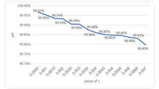
Figure 3: Average plr score of all 10,000 images from the CIFAR10 dataset, computed on our VGG16 model as a function of $\epsilon$.

Running the experiment took less than 400 minutes, and the algorithm completed successfully (i.e., did not fail) on 82% of the queries. We note here that Algorithm 1 naturally lends itself to parallelization, as each perturbed input can be evaluated independently of the others; we leave adding these capabilities to our proof-of-concept implementation for future work.

Experiment 2: Measuring robustness sensitivity to training epochs. In this experiment, we wanted to measure the sensitivity of the model’s robustness to the number of epochs in the training process. We ran Algorithm 1 (with $\delta=60\%,\epsilon=0.04,n=1,000$) on a VGG16 model trained with a different number of epochs — computing the average plr scores on all 10,000 images from CIFAR10 test set. The computed plr values are plotted as a function of the number of epochs in Figure 4. The results indicate that additional training leads to improved probabilistic local robustness. These results are also in line with previous work [27].

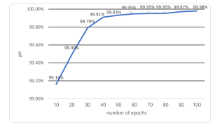
Figure 4: Average plr score of all 10,000 images from CIFAR10 test set, computed on VGG16 model as a function of training epochs.

Experiment 3: Categorial robustness. For our final experiment, we focused on categorial robustness, and specifically on comparing the robustness scores across categories. We ran Algorithm 1 ($\delta$ = 60%, $\epsilon=0.04$, and $n=1,000$) on our VGG16 model, for all 10,000 CIFAR10 test set images. The results, divided by category, appear in Table 5. For each category we list the average $plr$ score, the standard deviation of the data (which indicates the scattering for each category), and the probability of an adversarial input (the “Adv” column, calculated as $1-plr$). Performing this experiment took 37 minutes. Algorithm 1 completed successfully on 90.48% of the queries.

The results expose an interesting insight, namely the high variability in robustness between the different categories. For example, the probability of encountering an adversarial input for inputs classified as Cats is four times greater than the probability of encountering an adversarial input for inputs classified as Trucks. We observe that the standard deviation for these two categories is very small, which indicates that they are “far apart” — the difference between Cats and Trucks, as determined by the network, is generally greater than the difference between two Cats or between two Trucks. To corroborate this, we applied a T-test and a binomial test; and these tests produced a similarity score of less than 0.1%, indicating that the two categories are indeed distinctly different. The important conclusion that we can draw is that the per-category robustness of models can be far from uniform.

Figure 5: An analysis of average, per-category robustness, computed over all 10,000 images from the CIFAR10 dataset.

Category	plr	Std-Dev.	Adv
Airplane	$99.143\%$	$5.18\%$	$0.857\%$
Automotive	$99.372\%$	$3.86\%$	$0.628\%$
Bird	$97.226\%$	$8.87\%$	$2.774\%$
Cat	$97.112\%$	$8.77\%$	$2.888\%$
Deer	$98.586\%$	$6.25\%$	$1.414\%$
Dog	$97.233\%$	$8.58\%$	$2.767\%$
Frog	$98.524\%$	$6.39\%$	$1.476\%$
Horse	$98.606\%$	$6.09\%$	$1.394\%$
Ship	$98.389\%$	$6.63\%$	$1.611\%$
Truck	$99.390\%$	$4.26\%$	$0.610\%$

It is common in certification methodology to assign each sub-system a different robustness objective score, depending on the sub-system’s criticality [10]. Yet, to the best of our knowledge, this is the first time such differences in neural networks’ categorial robustness have been measured and reported. We believe categorial robustness could affect DNN certification efforts, by allowing engineers to require separate robustness thresholds for different categories. For example, for a traffic sign recognition DNN, a user might require a high robustness score for the “stop sign” category, and be willing to settle for a lower robustness score for the “parking sign” category.

5 Summary and Discussion

In this paper, we introduced RoMA — a novel statistical and scalable method for measuring the probabilistic local robustness of a black-box, high-scale DNN model. We demonstrated RoMA’s applicability in several aspects. The key advantages of RoMA over existing methods are: (i) it uses a straightforward and intuitive statistical method for measuring DNN robustness; (ii) scalability; and (iii) it works on black-box DNN models, without assumptions such as Lipschitz continuity constraints. Our approach’s limitations stem from the dependence on the normal distribution of the perturbed inputs, and its failure to produce a result when the Box-Cox transformation does not normalize the data.

The plr scores computed by RoMA indicate the risk of using a DNN model, and can allow regulatory agencies to conduct risk mitigation procedures: a common practice for integrating sub-systems into safety-critical systems. The ability to perform risk and robustness assessment is an important step towards using DNN models in the world of safety-critical applications, such as medical devices, UAVs, automotive, and others. We believe that our work also showcases the potential key role of categorial robustness in this endeavor.

Moving forward, we intend to: (i) evaluate our tool on additional norms, beyond $L_{\infty}$; (ii) better characterize the cases where the Box-Cox transformation fails, and search for other statistical tools can succeed in those cases; and (iii) improve the scalability of our tool by adding parallelization capabilities.

Acknowledgments. We thank Dr. Pavel Grabov From Tel-Aviv University for his valuable comments and support.

References

- [1] Anderson, B., Sojoudi, S.: Data-Driven Assessment of Deep Neural Networks with Random Input Uncertainty (2020), Technical Report. http://arxiv.org/abs/2010.01171
- [2] Anderson, T.: Anderson-Darling Tests of Goodness-of-Fit. Int. Encyclopedia of Statistical Science 1, 52–54 (2011)
- [3] Bastani, O., Ioannou, Y., Lampropoulos, L., Vytiniotis, D., Nori, A., Criminisi, A.: Measuring Neural Net Robustness with Constraints. In: Proc. 30th Conf. on Neural Information Processing Systems (NIPS) (2016)
- [4] Berlinger, M., Kolling, S., Schneider, J.: A Generalized Anderson-Darling Test for the Goodness-of-Fit Evaluation of the Fracture Strain Distribution of Acrylic Glass. Glass Structures & Engineering 6(2), 195–208 (2021)
- [5] Box, G., Cox, D.: An Analysis of Transformations Revisited, Rebutted. Journal of the American Statistical Association 77(377), 209–210 (1982)
- [6] Carlini, N., Wagner, D.: Towards Evaluating the Robustness of Neural Networks. In: Proc. 2017 IEEE Symposium on Security and Privacy (S&P). pp. 39–57 (2017)
- [7] Cohen, J., Rosenfeld, E., Kolter, Z.: Certified Adversarial Robustness via Randomized Smoothing. In: Proc. 36th Int. Conf. on Machine Learning (ICML) (2019)
- [8] Dvijotham, K., Garnelo, M., Fawzi, A., Kohli, P.: Verification of Deep Probabilistic Models (2018), Technical Report. http://arxiv.org/abs/1812.02795
- [9] European Union Aviation Safety Agency: Artificial Intelligence Roadmap: A Human-Centric Approach To AI In Aviation (2020), https://www.easa.europa.eu/newsroom-and-events/news/easa-artificial-intelligence-roadmap-10-published
- [10] Federal Aviation Administration: RTCA, Inc., Document RTCA/DO-178B (1993), https://nla.gov.au/nla.cat-vn4510326
- [11] Goodfellow, I., Shlens, J., Szegedy, C.: Explaining and Harnessing Adversarial Examples (2014), technical Report. http://arxiv.org/abs/1412.6572
- [12] Griffith, D., Amrhein, C., Huriot, J.M.: Econometric Advances in Spatial Modelling and Methodology: Essays in honour of Jean Paelinck. Springer Science & Business Media (2013)
- [13] Hammersley, J.: Monte Carlo Methods. Springer Science & Business Media (2013)
- [14] Huang, C., Hu, Z., Huang, X., Pei, K.: Statistical Certification of Acceptable Robustness for Neural Networks. In: Proc. Int. Conf. on Artificial Neural Networks (ICANN). pp. 79–90 (2021)
- [15] Katz, G., Barrett, C., Dill, D., Julian, K., Kochenderfer, M.: Reluplex: An Efficient SMT Solver for Verifying Deep Neural Networks. In: Proc. 29th Int. Conf. on Computer Aided Verification (CAV). pp. 97–117 (2017)
- [16] Katz, G., Barrett, C., Dill, D., Julian, K., Kochenderfer, M.: Reluplex: a Calculus for Reasoning about Deep Neural Networks. Formal Methods in System Design (FMSD) (2021)
- [17] Landi, A., Nicholson, M.: ARP4754A/ED-79A-Guidelines for Development of Civil Aircraft and Systems-Enhancements, Novelties and Key Topics. SAE Int. Journal of Aerospace 4, 871–879 (2011)
- [18] Levy, N., Katz, G.: RoMA: Code and Experiments (2022), https://drive.google.com/drive/folders/1hW474gRoNi313G1_bRzaR2cHG5DLCnJl
- [19] Mangal, R., Nori, A., Orso, A.: Robustness of Neural Networks: A Probabilistic and Practical Approach. In: Proc. 41st IEEE/ACM Int. Conf. on Software Engineering: New Ideas and Emerging Results (ICSE-NIER). pp. 93–96 (2019)
- [20] Michelmore, R., Kwiatkowska, M., Gal, Y.: Evaluating Uncertainty Quantification in End-to-End Autonomous Driving Control (2018), Technical Report. http://arxiv.org/abs/1811.06817
- [21] Pereira, A., Thomas, C.: Challenges of Machine Learning Applied to Safety-Critical Cyber-Physical Systems. Machine Learning and Knowledge Extraction 2(4), 579–602 (2020)
- [22] Rossi, R.: Mathematical Statistics: an Introduction to Likelihood Based Inference. John Wiley & Sons (2018)
- [23] Scipy: Scipy Python package (2021), https://scipy.org
- [24] Taherdoost, H.: Sampling Methods in Research Methodology; how to Choose a Sampling Technique for Research. Int. Journal of Academic Research in Management (IJARM) (2016)
- [25] Tit, K., Furon, T., Rousset, M.: Efficient Statistical Assessment of Neural Network Corruption Robustness. In: Proc. 35th Conf. on Neural Information Processing Systems (NeurIPS) (2021)
- [26] Vidot, G., Gabreau, C., Ober, I., Ober, I.: Certification of Embedded Systems Based on Machine Learning: A Survey (2021), Technical Report. http://arxiv.org/abs/2106.07221
- [27] Webb, S., Rainforth, T., Teh, Y., Kumar, M.: A Statistical Approach to Assessing Neural Network Robustness (2018), Technical Report. http://arxiv.org/abs/1811.07209
- [28] Weng, L., Chen, P.Y., Nguyen, L., Squillante, M., Boopathy, A., Oseledets, I., Daniel, L.: PROVEN: Verifying Robustness of Neural Networks with a Probabilistic Approach. In: Proc. 36th Int. Conf. on Machine Learning (ICML) (2019)
- [29] Yeo, I.K., Johnson, R.: A New Family of Power Transformations to Improve Normality or Symmetry. Biometrika 87(4), 954–959 (2000)