WimPyDD: an object-oriented Python code for WIMP-nucleus scattering direct detection in virtually any scenario

Abstract

We introduce WimPyDD, a modular, object–oriented and customisable Python code that accurately predicts the expected WIMP-nucleus scattering rates in WIMP direct–detection experiments including the response of the detector. WimPyDD utilises the framework of Galilean–invariant non–relativistic effective theory, allowing to handle an arbitrary number of effective operators, and can perform the calculation of the excepted rate in virtually any scenario, including inelastic scattering, WIMPs with an arbitrary spin, and a generic velocity distribution in the Galactic halo. The power and flexibility of WimPyDD is discussed in some explicit examples.

1 Introduction

Weakly Interacting Massive Particles (WIMPs) provide the most popular candidate of dark matter (DM) and there are various direct detection (DD) experiments searching for WIMP-nuclei scattering events in underground laboratories. Basically, the calculation of DD signals depends on different inputs coming from particle physics, nuclear physics, and astrophysics. Additionally, the realistic prediction from experiments require energy resolution, efficiency and the specific response to the target materials such as quenching. We introduce WimPyDD [1], a customisable, object-oriented Python code that allows to take all such inputs into account and predicts accurately the expected rate in an experiments virtually in any scenario, including WIMPs of arbitrary spin, inelastic scattering, and a generic velocity distribution of WIMP in the Galactic halo.

WimPyDD works in the framework of non-relativistic effective field theory (NREFT) for spin-1/2 [2] as well as arbitrary spin of DM [3]. While calculating the expected rate in an experiment WimPyDD factorizes the calculation into three parts namely i) the Wilson coefficients that depends on the model parameters; ii) a response function that depends on experimental inputs and nuclear physics; iii) the halo function that contains inputs from astrophysics and depends on WIMP velocity distribution. It is only at the last step that all of these factorised calculations are combined to calculate the expected number of events.

2 Scattering rate

The expected number of WIMP events in a DD experiment in the interval of visible energy $E_{1}^{\prime}\leq E^{\prime}\leq E_{2}^{\prime}$ can be written in the form [4],

$$R_{[E_{1}^{\prime},E_{2}^{\prime}]}(t)=\frac{\rho_{\chi}}{m_{\chi}}\int_{v_{T^{*}}}^{\infty}\sum_{T}dv{\cal R}_{T,[E_{1}^{\prime},E_{2}^{\prime}]}(v)\eta(v,t),$$ (1)

where $\rho_{\chi}$ is the local WIMP density, $m_{\chi}$ the WIMP mass, $T$ is the sum over the nuclear targets, and,

$$v_{T^{*}}\equiv\left\{\begin{aligned} \sqrt{\frac{2\delta}{\mu_{\chi T}}},\quad\text{if}\;\delta>0\\ 0,\quad\text{if}\;\delta\leq 0\,,\end{aligned}\right.$$ (2)

where $\delta$ is WIMP mass splitting and $\mu_{\chi T}$ is WIMP-nucleus reduced mass. The halo function in the expression above is,

$$\eta(v,t)=\int_{v}^{\infty}\frac{f(v^{\prime},t)}{v^{\prime}}\,dv^{\prime},$$ (3)

which depends on the WIMP speed distribution through $f(v,t)\equiv 1/(4\pi)\int d\Omega{v^{\prime}}^{2}f(\vec{v}^{\prime},t)$. In WimPyDD the speed distribution is utilised in terms of a superposition of $N_{s}$ streams,

$$f(v,t)=\sum_{k}^{N_{s}}\lambda_{k}(t)\delta(v-v_{k}).$$ (4)

Using the expression above the expected rate in an experiment can be written as,

$$R_{[E_{1}^{\prime},E_{2}^{\prime}]}(t)=\frac{\rho_{\chi}}{m_{\chi}}\sum_{k=1}^{N_{s}}\delta\eta_{k}(t)\int_{v_{T^{*}}}^{v_{i}}\sum_{T}dv{\cal R}_{T,[E_{1}^{\prime},E_{2}^{\prime}]}(v),$$ (5)

where $\delta\eta_{k}(t)=\lambda_{k}(t)/v_{k}$. Since most of the DD experiments put upper bound on the time average of $R_{[E_{1}^{\prime},E_{2}^{\prime}]}(t)$, we have,

$$S^{(0)}_{[E_{1}^{\prime},E_{2}^{\prime}]}\equiv\frac{1}{T_{0}}\int_{0}^{T_{0}}R_{[E_{1}^{\prime},E_{2}^{\prime}]}(t)dt,$$ (6)

with $T_{0}=1$ year, utilising which we arrived on the master formula used by WimPyDD,

$$S^{(0)}_{[E_{1}^{\prime},E_{2}^{\prime}]}=\frac{\rho_{\chi}}{m_{\chi}}\sum_{k=1}^{N_{s}}\delta\eta_{k}^{(0)}\times\sum_{T}\sum_{ij}\sum_{\tau\tau^{\prime}}c_{j}^{\tau}(w_{i},q_{0})c_{k}^{\tau^{\prime}}(w_{i},q_{0}^{\prime})$$

$$\left\{\left[\bar{{\cal R}}^{0}_{T,[E_{1}^{\prime},E_{2}^{\prime}]}\right]_{jk}^{\tau\tau^{\prime}}(E_{R})+(\frac{v_{k}^{2}}{c^{2}}-\frac{\delta}{\mu_{\chi T}})\left[\bar{{\cal R}}^{1}_{T,[E_{1}^{\prime},E_{2}^{\prime}]}\right]_{jk}^{\tau\tau^{\prime}}(E_{R})\right.$$

$$\left.-\frac{m_{T}}{2\mu_{\chi T}^{2}}\left[\bar{{\cal R}}^{1E}_{T,[E_{1}^{\prime},E_{2}^{\prime}]}\right]_{jk}^{\tau\tau^{\prime}}(E_{R})-\frac{\delta^{2}}{2m_{T}}\left[\bar{{\cal R}}^{1E^{-1}}_{T,[E_{1}^{\prime},E_{2}^{\prime}]}\right]_{jk}^{\tau\tau^{\prime}}(E_{R})\right\}^{E_{R}^{max}(v_{k})}_{E_{R}^{min}(v_{k})},$$

where $\{f(E_{R})\}_{E_{1}}^{E_{2}}\equiv f(E_{2})-f(E_{1})$ and integrated response functions $\bar{{\cal R}}_{T}$ are explicitly provided in [1].

3 WimPyDD

WimPyDD is available at the following webpage,

       https://wimpydd.hepforge.org     

where the code and additional explanations are available. The latest version of WimPyDD can be installed using,

     git clone https://phab.hepforge.org/source/WimPyDD.git     or can be directly downloaded from WimPyDD’s homepage. This will create a folder WimPyDD. There are standard libraries required by WimPyDD such as matplotlib, numpy, scipy, and pickle. To use WimPyDD the user has to import it using, for instance,

     import WimPyDD as WD     

3.1 Signal routines

There are three main routines in WimPyDD that calculate the differential cross section $(d\sigma/dE_{R})_{T}$, the differential rate $dR/dE_{R}$, and the integrated rate of Eq. (1).

To calculate the differential cross section $(d\sigma/dE_{R})_{T}$ (in cm²/keV) use,

       WD.dsigma_der(element_obj,hamiltonian_obj,mchi,v,er,**args)     with mchi the WIMP mass $m_{\chi}$ in GeV, v the WIMP incoming speed $v$ in km/sec, er the recoil energy in keV, and where element_obj defines a nuclear target $T$ while hamiltonian_obj defines an effective Hamiltonian. To evaluate the differential rate $dR/dE_{R}$ use,

       WD.diff_rate(target_obj,hamiltonian_obj,mchi,
    energy,vmin,delta_eta, **args)     where target_obj is either a single element or a combination of elements with stoichiometric coefficients, vmin and delta_eta are two arrays containing the $v_{k}$ and $\delta\eta_{k}^{(0)}$ in km/s and (km/s)^-1, respectively. The routine streamed_halo_function is provided in WimPyDD for calculating them. The expected rate including the response of the detector is calculated by the routine,

       WD.wimp_dd_rate(exp_obj, hamiltonian_obg, vmin,
    delta_eta, mchi,**args)     

where exp_obj is instantiated by the experiment class and contains all the required information about the experimental set-up, including the energy bins where the rate is integrated. There are two arrays produced as an output of this routine with the centers of energy bins and the corresponding expected rates calculated using Eq. (LABEL:eq:rate_rbar_inelastic).

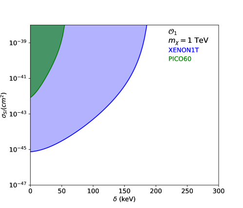
Figure 1: Exclusion limits on WIMP-nucleon SI scattering cross-section as a function of mass splitting $\delta$ at 90% confidence for XENON1T [5] and PICO60 [6] experiments. We considered $m_{\chi}=1$ TeV and a WIMP escape velocity $v_{\rm esc}=550$ km/s in the Galactic rest frame.

3.2 Example

In the present section we introduce the potentialities of WimPyDD by explicitly showing example of WIMP-nucleus inelastic scattering.

3.2.1 Inelastic scattering

Let’s set up the following effective Hamiltonian for spin-independent (SI) interaction $\mathcal{O}_{1}$,

$${\cal H}=c_{1}^{0}{\cal O}_{1}t^{0}+c_{1}^{1}{\cal O}_{1}t^{1}=\sqrt{\frac{\sigma_{SI}\pi}{\mu^{2}_{\chi p}\hbar^{2}c^{2}}}[(1+r){\cal O}_{1}t^{0}+(1-r){\cal O}_{1}t^{1}].$$ (8)

We utilised $c^{0}_{1}=c^{p}_{1}(1+r)$ and $c^{1}_{1}=c^{p}_{1}(1-r)$ with $r=c^{n}_{1}/c^{p}_{1}$, where $c^{p}_{1}$ and $c^{n}_{1}$ are the WIMP couplings to the proton and the neutron respectively. We replaced $c^{p}_{1}$ following,

$$c^{p}_{1}=\sqrt{\frac{\sigma_{SI}\pi}{\mu^{2}_{\chi p}\hbar^{2}c^{2}}}.$$ (9)

In the expression above $\sigma_{SI}=(c_{1}^{p}\mu_{\chi p})^{2}/\pi$ is the WIMP-nucleon cross-section while $\mu_{\chi p}$ is the WIMP-nucleon reduced mass. This is implemented in WimPyDD as following,

     def wc(mchi,cross_section,r):
      hbarc2=0.389e-27
      mn=0.931
      mu=mchi*mn/(mchi+mn)
      cp=(np.pi*cross_section/(mu**2*hbarc2))**(1./2.)
      return cp*np.array([1.+r,1.-r])
      
  SI=WD.eft_hamiltonian(’SI’,{1: wc})     As discussed the WimPyDD code provides a simple routine mchi_vs_exclusion that allows to estimate the upper bound on any parameter for which exclusion cross-section is chosen. The cross-section can be factorised from the rate by simply comparing the output of wimp_dd_rate with $\sigma_{SI}=1$ cm² to the experimental upper bounds on the count rate in each energy bin of the considered experiment and taking the most stringent constraint. In mchi_vs_exclusion we did not pass the $\sigma_{SI}$ argument so that it is set to 1 by default. The mass splitting $\delta$ goes as an input to the routine mchi_vs_exclusion and the exclusion cross-section is scanned in terms of $\delta$ for XENON1T [5] and PICO60 [6] experiments as following,

     delta_vec=np.linspace(0.1,300,100)
  WD.load_response_functions(WD.XENON_1T_2018,SI)
  WD.load_response_functions(WD.PICO60_2019,SI)
  vmin,delta_eta=
  WD.streamed_halo_function(n_vmin_bin =1000, v_esc_gal=550)
    sigma_xenon=[WD.mchi_vs_exclusion(WD.XENON_1T_2018, SI, vmin,
  delta_eta, delta=delta, mchi_vec=np.array([1000]), 
  j_chi=0.5)[1] for delta in delta_vec]
  sigma_pico=[WD.mchi_vs_exclusion(WD.PICO60_2019, SI, vmin,
  delta_eta, delta=delta, mchi_vec=np.array([1000]), 
  j_chi=0.5)[1] for delta in delta_vec]
    pl.plot(delta_vec[:64],sigma_xenon[:64],’-b’)  pl.plot(delta_vec[:20],sigma_pico[:20],’-g’)     In Fig. 1 the exclusion plot for the cross-section $\sigma_{SI}$ is plotted as a function of the mass splitting $\delta$ for a WIMP escape velocity $v_{esc}$ = 550 km/s in the Galactic rest frame. We see that the current XENON1T and PICO60 constraints require $\delta$ to be $\sim$185 keV and $\sim$55 keV, respectively.

References

References

- [1] I. Jeong, S. Kang, S. Scopel and G. Tomar, [arXiv:2106.06207 [hep-ph]].
- [2] N. Anand, A. L. Fitzpatrick and W. C. Haxton, Phys. Rev. C 89, no.6, 065501 (2014) doi:10.1103/PhysRevC.89.065501 [arXiv:1308.6288 [hep-ph]].
- [3] P. Gondolo, S. Kang, S. Scopel and G. Tomar, Phys. Rev. D 104, no.6, 063017 (2021) doi:10.1103/PhysRevD.104.063017 [arXiv:2008.05120 [hep-ph]].
- [4] E. Del Nobile, G. Gelmini, P. Gondolo and J. H. Huh, JCAP 10, 048 (2013) doi:10.1088/1475-7516/2013/10/048 [arXiv:1306.5273 [hep-ph]].
- [5] E. Aprile et al. [XENON], Phys. Rev. Lett. 121, no.11, 111302 (2018) doi:10.1103/PhysRevLett.121.111302 [arXiv:1805.12562 [astro-ph.CO]].
- [6] C. Amole et al. [PICO], Phys. Rev. D 100, no.2, 022001 (2019) doi:10.1103/PhysRevD.100.022001 [arXiv:1902.04031 [astro-ph.CO]].