Sequential Modeling with Multiple Attributes for Watchlist Recommendation in E-Commerce

Abstract.

In e-commerce, the watchlist enables users to track items over time and has emerged as a primary feature, playing an important role in users’ shopping journey. Watchlist items typically have multiple attributes whose values may change over time (e.g., price, quantity). Since many users accumulate dozens of items on their watchlist, and since shopping intents change over time, recommending the top watchlist items in a given context can be valuable. In this work, we study the watchlist functionality in e-commerce and introduce a novel watchlist recommendation task. Our goal is to prioritize which watchlist items the user should pay attention to next by predicting the next items the user will click. We cast this task as a specialized sequential recommendation task and discuss its characteristics. Our proposed recommendation model, Trans2D, is built on top of the Transformer architecture, where we further suggest a novel extended attention mechanism (Attention2D) that allows to learn complex item-item, attribute-attribute and item-attribute patterns from sequential-data with multiple item attributes. Using a large-scale watchlist dataset from eBay, we evaluate our proposed model, where we demonstrate its superiority compared to multiple state-of-the-art baselines, many of which are adapted for this task.

1. Introduction

The watchlist, a collection of items to track or follow over time, has become a prominent feature in a variety of online applications spanning multiple domains, including news reading, television watching, and stock trading. One domain in which watchlists have become especially popular is e-commerce, where they allow users to create personalized collections of items they consider to purchase and save them in their user account for future reference. Saving items in the watchlist allows users to track a variety of dynamic characteristics over relatively long period of times. These include the price and related deals, shipping costs, delivery options, etc.

A user’s watchlist can be quite dynamic. At any moment, the user may choose to revise her watchlist by adding new items (e.g., after viewing an item’s page) or removing existing items (e.g., the user has lost her interest in an item). Over time, item attributes may change (e.g., an item’s price has dropped) or items may become invalid for recommendation (e.g., an item has been sold out). User’s latest shopping journey may change as well, as she may show interest in other items, categories or domains.

All in all, in between two consecutive interactions with the watchlist, the user may change her priority of which next item to pay attention to. Considering the fact that the watchlist of any user may include dozens of items, it may be quite overwhelming for users to keep track of all changes and opportunities related to their watchlist items. Given a limited number of items that can be displayed to the user (e.g., 2-3 items on eBay’s mobile homepage watchlist module) and the dynamic nature of watchlist items, our goal is, therefore, to help users prioritize which watchlist items they should pay attention to next.

We cast the watchlist recommendation (hereinafter abbreviated as WLR) task as a specialized sequential recommendation (SR) task. Given the historical interactions of a user with items, the goal of the SR task is to predict the next item the user will interact with (Wang et al., 2019). While both tasks are related to each other, we next identify two important characteristics of the WLR task.

The first characteristic of the WLR task is that, at every possible moment in time, only a subset of items, explicitly chosen to be tracked by the user prior to recommendation time, should be considered. Moreover, the set of items in a given user’s watchlist may change from one recommendation time to another. Yet, most previous SR studies assume that, the user’s next interaction may be with any possible item in the catalog. Therefore, the main focus in such works is to predict the next item’s identity. The WLR task, on the other hand, aims to estimate the user’s attention to watchlist items by predicting the click likelihood of each item in the user’s watchlist. Noting that watchlist datasets may be highly sparse, as in our case, representing items solely by their identity usually leads to over-fit. A better alternative is to represent items by their attributes. Yet, to the best of our knowledge, only few previous SR works can consider attribute-rich inputs both during training and prediction.

The second characteristic of the task lies in the important observation that, possible shifts in the user’s preferences towards her watched items may be implied by her recently viewed items (RVIs). For example, a user that tracks a given item in her watchlist, may explore alternative items (possibly not in her watchlist) from the same seller or category, prior to her decision to interact with the tracked item (e.g., the watched item price is more attractive).

Trying to handle the unique challenges imposed by the WLR task, we design an extension to the Transformer model (Vaswani et al., 2017). Our proposed Transformer model, Trans2D, employs a novel attention mechanism (termed Attention2D) that allows to learn complex preferential patterns from historical sequences of user-item interactions accompanied with a rich and dynamic set of attributes. The proposed attention mechanism is designed to be highly effective, and requires only a small addition to the model’s parameters.

Using a large-scale user watchlist dataset from eBay, we evaluate the proposed model. We show that, by employing the novel Attention2D mechanism within the Transformer model, our model can achieve superior recommendation performance, compared to a multitude of state-of-the-art SR models, most of which we adapt to this unique task.

2. Related Work

The watchlist recommendation (WLR) task can be basically viewed as a specialization of the sequential recommendation (SR) task. The majority of previous SR works assume that the input sequence includes only item-IDs (Wang et al., 2019) and focus on predicting the identity of the next item that the user may interact with (Wang et al., 2019). Notable works span from Markov-Chain (MC) (Rendle et al., 2010) and translation-based (He et al., 2017) models that aim to capture high-order relationships between users and items, to works that employ various deep-learning models that capture user’s evolving preferences such as RNNs (e.g., GRU (Hidasi et al., 2016a; Tan et al., 2016)), CNNs (e.g., (Tang and Wang, 2018; Tuan and Phuong, 2017)), and more recent works that utilize Transformers (e.g., SASRec (Kang and McAuley, 2018), BERT4Rec (Sun et al., 2019) and SSE-PT (Wu et al., 2020)).

Similar to (Kang and McAuley, 2018; Sun et al., 2019; Wu et al., 2020), we also utilize the Transformer architecture. Yet, compared to existing works that train models to predict the next item-ID, our model is trained to rank watchlist items according to their click likelihood. The main disadvantage of models that focus on item-ID only inputs is their inability to handle datasets having items with high sparsity and item cold-start issues. Utilizing rich item attributes, therefore, becomes extremely essential for overcoming such limitations, and specifically in our task. By sharing attribute-representations among items, such an approach can better handle sparse data and item cold-start.

Various approaches for obtaining rich attribute-based item representations during training-time have been studied so far. This includes a variety of attribute representations aggregation methods (Mizrachi and Levin, 2019; Beutel et al., 2018; Sar Shalom et al., 2017, 2018) (e.g., average, sum, element-wise multiplication, etc.), concatenation (Mizrachi and Levin, 2019; Zhou et al., 2018; Chen et al., 2019), parallel processing (Hidasi et al., 2016b; Ren et al., 2020), usage of attention-based Transformer layer (Zhang et al., 2019) and graph-based representations (Wang and Cai, 2020). Furthermore, attributes have been utilized for introducing additional mask-based pre-training tasks (Zhou et al., 2020) (e.g., predict an item’s attribute).

Yet, during prediction, leveraging the attributes is not trivial, as the entire catalog should be considered. Indeed, all aforementioned works still utilize only item-IDs for prediction. For example, the S3 (Zhou et al., 2020) model, one of the leading self-supervised SR models, supports only static attributes, which are only considered during its pre-training phase. Hence, extending existing works for handling the WLR task, which requires to consider also item attributes at prediction time, is extremely difficult, and in some cases, is just impossible. As we shall demonstrate in our evaluation (Section 4), applying those previous works (Mizrachi and Levin, 2019; Sar Shalom et al., 2018; Chen et al., 2019; Zhang et al., 2019) that can be extended to handle the WLR task (some with a lot of effort and modification), results in inferior recommendation performance compared to our proposed model.

Few related works allow to include item attributes as an additional context that can be utilized for representing items both during training and prediction time. Such works either extend basic deep-sequential models (RNNs (Beutel et al., 2018; Smirnova and Vasile, 2017) and Transformers (Eshel et al., 2021)) with context that encodes attribute-rich features, or combine item-context with sequential data using Factorization Machines (Pasricha and McAuley, 2018; Chen et al., 2020).

Our proposed model is also capable of processing sequential inputs having multiple item attributes. To this end, our model employs a modified Transformer architecture with a novel attention mechanism (Attention2D) that allows to process complete sequences of 2D-arrays of data without the need to pre-process items (e.g., aggregate over attributes) in the embedding layer (as still need to be done in all previous works). This allows our model, with a slight expense of parameters, to capture highly complex and diverse preference signals, which are preserved until the prediction phase.

3. Recommendation Framework

3.1. Problem Formulation

The WLR task can be modeled as a special case of the sequential recommendation (SR) task (Wang et al., 2019), with the distinction that, at every possible moment, there is only a limited, yet dynamic, valid set of watched items that need to be considered. Using the user’s historical interactions with watchlist items and her recently viewed item pages (RVIs), our goal is, therefore, to predict which items in the current user’s watchlist will be clicked. A user’s click on a watchlist item usually implies that the user has regained her interest in that item. Moreover, we wish to leverage the fact that watched items are dynamic, having attributes whose values may change over time (e.g., price), and therefore, may imply on a change in user’s preferences.

Formally, let $\mathbf{I}$ be the set of all recommendable items. For a given user $u$, let $\mathbf{WL}_{t}\subseteq{\mathbf{I}}$ denote the set of items in the user’s watchlist prior to the time of $t$-th click on any of the watchlist items, termed also hereinafter a “watchlist-snapshot”. We further denote $m_{t}=|\mathbf{WL}_{t}|$ the number of items in a given snapshot. A user may click on any item in $\mathbf{WL}_{t}$, which leads her to the item’s page; also termed a “view item” (VI) event. VI events may also occur independently of items in the user’s watchlist; e.g., the user views an item in $\mathbf{I}$ following some search result or directed to the item’s page through some other organic recommendation module, etc. Let $\mathbf{VI}_{t}\subseteq{\mathbf{I}}$, with $n_{t}=|\mathbf{VI}_{t}|$, denote a possible sequence of item pages viewed by user $u$ between the $t-1$-th and $t$-th clicks on her watchlist items, further termed a “view-snapshot”.

We next denote $\mathbf{S}(t)$ – the user’s history prior to her $t$-th interaction with the watchlist. $\mathbf{S}(t)$ is given by the sequence of the user’s previous clicks on watchlist items and items whose page the user has viewed in between each pair of consecutive clicks, i.e.:

$$\mathbf{S}(t)=\underbrace{w_{1}}_{click},\underbrace{v_{1,1},\ldots,v_{1,n_{1}}}_{\mathbf{VI}_{1}},\ldots,\underbrace{w_{t-1}}_{click},\underbrace{v_{t-1,1},\ldots,v_{t-1,n_{t-1}}}_{\mathbf{VI}_{t-1}}.$$

Here, $w$ denotes a single user’s click on some watchlist item, while $v$ denotes an item page viewed by the user. We note that, every watchlist item clicked by the user leads to the item’s page, hence: $w_{l}=v_{l,1}$ ($\forall{l}:1\leq{l}\leq{t-1}$).

Using the above definitions, for any given user history $\mathbf{S}(t)$ and new watchlist snapshot $\mathbf{WL}_{t}$ to consider, our goal is to predict which items in $\mathbf{WL}_{t}$ the user is mostly likely to click next. Therefore, at service time, we wish to recommend to the user the top-$k$ items in $\mathbf{WL}_{t}$ with the highest click likelihood.

3.2. Recommendation Model

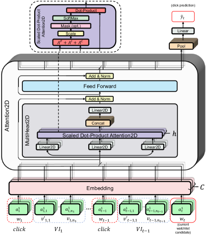
Figure 1. Watchlist recommendation model (Trans2D) using Transformer with Attention2D layer. The model has three main parts: Embedding layer (bottom-side), Attention2D layer (middle-side) and Prediction layer (upper-right side) The ScaledDotProductAttention2D component is further illustrated in the upper-left side.

Our WLR model, Trans2D, extends the Transformer (Vaswani et al., 2017) architecture for handling sequences with items that include several categorical attributes as in the case of watchlist items. Using such an architecture allows us to capture high-order dependencies among items and their attributes with a minimum loss of semantics and a reasonable model complexity. The model’s network architecture is depicted in Figure 1. The network includes three main layers, namely, Embedding layer, Attention2D layer and Prediction layer. We next describe the details of each layer.

3.3. Embedding Layer

A common modeling choice in most related literature (Wang et al., 2019), is to represent user’s sequence $\mathbf{S}(t)$ as the sequence of item-IDs. Let $N=\sum_{l=1}^{t-1}(1+n_{l})$ denote the total items in $\mathbf{S}(t)$. These item-IDs are typically embedded into a corresponding sequence of $d$-dimensional vectors $\mathbf{E}=(\mathbf{e}_{1},\ldots,\mathbf{e}_{N});\forall{i}:\mathbf{e}_{i}\in{\mathbb{R}}^{d}$ using an embedding dictionary and serve as input representation to neural-network models. However, such a representation has two main disadvantages. Firstly, it is prone to cold-start problems as items that never appear during training must be discarded or embedded as an ‘unknown’ item. Secondly, items that only appear once or a few times during training are at high risk of over-fitting by the training process memorizing their spurious labels. Such sparsity issues are particularly present in our data (as will be discussed in Section 4.1), prompting us to represent an item as a collection of attributes, rather than an item-ID. Such an approach is less prone to sparsity and over-fitting, as the model learns to generalize based on item-attributes.

Following our choice for item representation, we now assume that each item in $\mathbf{S}(t)$ is represented by $C$ attributes: $[a_{1},\ldots,a_{C}]$. Therefore, the input to our model is a 2D-array of item attributes $\mathbf{S}(t)=[a]_{i,j}$; where $i\in[1,\ldots,N],j\in[1,\ldots,C]$. Hereinafter, we refer to the first axis of $\mathbf{S}(t)$ as the sequence (item) dimension and its second axis as the channel (attribute) dimension.

The first layer of our model is an embedding layer with keys for all possible attribute values in our data. Therefore, by applying this layer on the user’s sequence $\mathbf{S}(t)$, we obtain a 2D-array of embedding vectors $\mathbf{E}=[e]_{i,j}=Embd([a]_{i,j})$. Note that, since each item attribute embedding by itself is a $d$-dimensional vector, $\mathbf{E}\in{\mathbb{R}}^{N\times{C}\times{d}}$ is a 3D-array. $\mathbf{E}$ is next fed into a specially modified Transformer layer which is our model’s main processing layer.

3.4. Modified Transformer

Most existing SR models (e.g., (Hidasi et al., 2016a; Tang and Wang, 2018; Kang and McAuley, 2018; Sun et al., 2019)) take a sequence of vectors as input. However, in our case, we do not have a 1D-sequence of vectors but rather a 2D-array representing a sequence of ordered attribute collections. As Transformers were shown to demonstrate state-of-the-art performance in handling sequential data in general (Vaswani et al., 2017) and sequential recommendation data specifically (Kang and McAuley, 2018; Sun et al., 2019; Zhou et al., 2020; Wu et al., 2020; Eshel et al., 2021), we choose to employ Transformers and extend the Attention Mechanism of the Transformer to handle 2D-input sequences, rather than a 1D-input sequence.

Since the vanilla attention model employed by existing Transformer architectures cannot be directly used for 2D-data, different pooling techniques were devised to reduce the channel dimension and produce a 1D-sequence as an input for the Transformer. For example, in BERT (Kenton and Toutanova, 2019), token, position and sentence embeddings are summed before being fed into the Transformer Encoder. Other alternatives to summation were explored such as averaging, concatenation, or a secondary Transformer layer (e.g., (Chen et al., 2019; Zhang et al., 2019)). Yet, most of these approaches suffer from a reduction in data representation happening prior to applying the attention workhorse. This makes it harder for the attention mechanism to learn rich attention patterns. An exception is the concatenation approach that sidesteps this problem but produces very long vectors, which in turn, requires Transformer layers to have a large input dimension making them needlessly large. As an alternative, we next propose Attention2D – a dedicated novel attention block that is natively able to handle 2D-inputs in an efficient way. Such an extended attention mechanism will allow us to learn better attention patterns without significantly increasing the architecture size.

3.5. Attention2D

We now describe in detail our modified attention block, referred to as Attention2D. For comparison to the vanilla Transformer model, we encourage the reader to refer to (Vaswani et al., 2017). An attention block maps a query ($\mathbf{Q}$) and a set of key ($\mathbf{K}$) - value ($\mathbf{V}$) pairs to an output, where the query, keys, values, and output are all vectors (Vaswani et al., 2017). The Attention2D block in turn receives a 2D-array of vectors, representing a sequence of ordered item attribute collections and computes the attention between all item-attributes while enabling different semantics per channel to better capture both channel interactions and differences. This way, one attribute of a specific item can influence another attribute of a different item regardless of other attributes, making it possible to learn high-order dependencies between different items and attributes. For instance, in our usecase, the price preferences of a user, captured by the price channel can be computed using attention both to previously clicked item prices and to past viewed items of sellers correlated with pricey or cheap items. The full Attention2D block is illustrated in Figure 1. We now provide a detailed description of its implementation.

3.5.1. Linear2D

The input to our model is a 2D-array of input vectors, generally denoted hereinafter $\mathbf{X}=[\mathbf{x}]_{i,j}$ (and specifically in our model’s input $\mathbf{X}=\mathbf{E}$). Our model requires operations acting on such 2D-arrays throughout. To this end, we first define two extensions of standard linear neural-network layers:

(1) $$\begin{split}{Linear2D}_{W}(\mathbf{X})=\mathbf{W}_{j}[\mathbf{x}]_{i,j}\\ {Linear2D^{+}}_{W,b}(\mathbf{X})=\mathbf{W}_{j}[\mathbf{x}]_{i,j}+b_{j},\end{split}$$

where $\mathbf{W}=[W_{1},\ldots,W_{C}];b=[b_{1},\ldots,b_{C}]$ and $\mathbf{W}_{j}\in{\mathbb{R}}^{d\times d};b_{j}\in{\mathbb{R}}^{d}$ are trainable parameters per channel $1\leq j\leq C$. These operations define a linear layer (with or without bias) with different trainable parameters per channel and shall allow the model to facilitate interactions between different channels while preserving the unique semantics of each channel.

We start by mapping our input ($\mathbf{E}$) into three 2D-arrays of query $\mathbf{Q}=[\mathbf{q}]_{i,j}$, key $\mathbf{K}=[\mathbf{k}]_{i,j}$ and value $\mathbf{V}=[\mathbf{v}]_{i,j}$ vectors corresponding to each input. We do so by applying three Linear2D layers:

$$\mathbf{Q}={Linear2D}_{Q}(\mathbf{E})\ ;\ \mathbf{K}={Linear2D}_{K}(\mathbf{E})\ ;\ \mathbf{V}={Linear2D}_{V}(\mathbf{E})$$

3.5.2. ScaledDotProductAttention2D

We next describe the core part of our proposed attention mechanism, which is used to compute a transformed representation of our 2D-input array. This part is further illustrated on the upper-left side of Figure 1. For brevity of explanation, we consider a single query vector $[\mathbf{q}]_{i,j}\in{\mathbf{Q}}$ and key vector $[\mathbf{k}]_{i^{\prime},j^{\prime}}\in{\mathbf{K}}$, while in practice, this operation is performed for every $i,i^{\prime}\in[1,\ldots,N]$ and $j,j^{\prime}\in[1,\ldots,C]$.

First, we compute the following three attention scores (where $T$ here denotes the matrix transpose operation):

$$\mathbf{A}_{i,j,i^{\prime},j^{\prime}}^{F}=[\mathbf{q}]_{i,j}\cdot[\mathbf{k}]^{T}_{i^{\prime},j^{\prime}}\ ;\ \ \mathbf{A}_{i,i^{\prime}}^{I}=\sum_{z=1}^{C}[\mathbf{q}]_{i,z}\cdot[\mathbf{k}]^{T}_{i^{\prime},z}\ ;$$

$$\mathbf{A}_{j,j^{\prime}}^{C}=\sum_{z=1}^{N}[\mathbf{q}]_{z,j}\cdot[\mathbf{k}]^{T}_{z,j^{\prime}}$$

where:

$\bullet$ $\mathbf{A}^{F}$ is a 4D-array of attention scores between all inputs as the dot-product between every query vector and every key vector. This attention corresponds to the attention scores in a vanilla attention layer between any two tokens, yet with the distinction that in our case we have 2D-inputs.

$\bullet$ $\mathbf{A}^{I}$ is a matrix of attention scores between whole items in our input, computed as the marginal attention over all channels. This attention captures the importance of items to each other regardless of a particular channel.

$\bullet$ $\mathbf{A}^{C}$ is a matrix of attention scores between channels in our input, computed as the marginal attention over all items. This attention captures the importance of channels to each other regardless of a particular item.

The attention scores are further combined using their weighted sum:

(2) $$\mathbf{A}_{i,j,i^{\prime},j^{\prime}}=\alpha_{1}*\mathbf{A}^{F}_{i,j,i^{\prime},j^{\prime}}+\alpha_{2}*\mathbf{A}^{I}_{i,i^{\prime}}+\alpha_{3}*\mathbf{A}_{j,j^{\prime}}^{C},$$

where $\alpha_{1},\alpha_{2},\alpha_{3}$ are learned scalars, denoting the relative importance of each attention variant, respectively.

The result of this step is, therefore, a 4D-array $\mathbf{A}$ of attention scores from any position $(i,j)$ to every position $(i^{\prime},j^{\prime})$. Similarly to (Vaswani et al., 2017), we apply a softmax function over $\mathbf{A}$, with a scaling factor of $\sqrt{d}$, so that our scores will sum up to 1. We then compute the final transformed output $[\mathbf{o}]_{i,j}$ as a weighted average over all value vectors using the computed attention scores:

$$\mathbf{P}=softmax\left(\frac{\mathbf{A}}{\sqrt{d}}\right)\quad;\quad[\mathbf{o}]_{i,j}=\sum_{i^{\prime},j^{\prime}}\mathbf{P}_{i,j,i^{\prime},j^{\prime}}[v]_{i^{\prime},j^{\prime}}$$

Finally, we can define our Attention2D layer as an attention layer that receives a triplet of $(\mathbf{Q},\mathbf{K},\mathbf{V})$ 2D-arrays of query, key and value vectors as its input and outputs a 2D-array transformed vectors:

(3) $$\begin{split}{ScaledDotProductAttention2D}(\mathbf{Q},\mathbf{K},\mathbf{V})=[\mathbf{o}]_{i,j}\\ i\in[1,\ldots,N],j\in[1,\ldots,C]\end{split}$$

The Attention2D layer allows each item-attribute to attend to all possible item-attributes in the input. To prevent unwanted attendance (such as accessing future information in the sequence), we mask it out by forcing the relevant (future) attention values to $-\infty$ before the softmax operation.

3.5.3. Multi-Head Attention2D

Similarly to (Vaswani et al., 2017), instead of performing a single attention function, we can apply $h$ different functions (“Attention-Heads”) over different sub-spaces of the queries, keys, and values. This allows to diversify the attention patterns that can be learned, helping to boost performance. For instance, one attention head can learn to focus on price-seller patterns, while another on different price-condition patterns. We facilitate this by applying $h$ different Linear2D layers, resulting in $h$ triplets of $(\mathbf{Q}_{r},\mathbf{K}_{r},\mathbf{V}_{r})$; on each, we apply the aforementioned ScaledDotProductAttention2D layer. We then concatenate all $h$ results and project it back to a $d$-dimensional vector using another Linear2D layer:

(4) $$\begin{split}{MultiHead2D}(\mathbf{Q},\mathbf{K},\mathbf{V})={Linear2D}_{W^{O}}(Concat(head_{1},...,head_{h}))\\ head_{r}={ScaledDotProductAttention2D}(\mathbf{Q}_{r},\mathbf{K}_{r},\mathbf{V}_{r})\\ \mathbf{Q}_{r}={Linear2D}_{Q_{r}}(\mathbf{Q})\ ;\ \mathbf{K}_{r}={Linear2D}_{K_{r}}(\mathbf{K})\ ;\ \mathbf{V}_{r}={Linear2D}_{V_{r}}(\mathbf{V})\\ \end{split}$$

3.5.4. Position-wise Feed-Forward Networks

We finally allow the Attention2D output to go through additional Linear2D layers in order to be able to cancel out unwanted applied alignments and learn additional complex representations:

$$FFN(\mathbf{X})={Linear2D^{+}}_{W^{2},b^{2}}(ReLU({Linear2D^{+}}_{W^{1},b^{1}}(\mathbf{X})))$$

3.5.5. Full Layer implementation

A full Attention2D block is combined from a MultiHead2D layer and then a FFN layer, where a residual connection (He et al., 2016) is applied around both, by adding the input to the output and applying a layer normalization (Ba et al., 2016), as follows:

(5) $$\begin{split}{Attention2D}(\mathbf{X})=LayerNorm(\mathbf{X}^{\prime}+FFN(\mathbf{X}^{\prime})),\\ \mathbf{X}^{\prime}=LayerNorm(\mathbf{X}+{MultiHead2D}(\mathbf{X},\mathbf{X},\mathbf{X}))\end{split}$$

After applying the Attention2D block, we end up with a transformed 2D-array of vectors $\mathbf{E}^{\prime}={Attention2D}(\mathbf{E})$, having the same shape as the original input. Therefore, Attention2D layers can be further stacked one on the other to achieve deep attention networks.

3.6. Prediction Layer

The final stage in our model is label (click/no-click) prediction. Let $w_{t}\in{\mathbf{WL}_{t}}$ be an item in the user’s watchlist whose click likelihood we wish to predict. To this end, as a first step, we append $w_{t}$ to $\mathbf{S}(t)$. We then feed the extended sequence to the Transformer and obtain $\mathbf{E}^{\prime}$, the transformed 2D-array representation based on our Attention2D block (see again Eq 5).

We predict the click likelihood of item $w_{t}$ based on its transformed output $e^{\prime}_{N+1}\in{\mathbb{R}}^{d\times C}$. For that, we first obtain a single representation of it by applying $Pool(e^{\prime}_{N+1})$ – a pooling layer over the channel dimension in $e^{\prime}_{N+1}$. While many pooling options may be considered, we use a simple average pooling. This is similar to the channel dimension reduction discussed in Section 3.4, but instead of applying the pooling before the attention mechanism, we are able to apply the pooling after the Attention2D block. This makes it possible for the Attention2D block to capture better attention patterns between different items and attributes.

Finally, we obtain the item’s predicted label (denoted $\hat{y}$) by applying a simple fully connected layer on $Pool(e^{\prime}_{N+1})$ to a single neuron representing the item’s click likelihood, as follows:

(6) $$\hat{y}=\sigma(\mathbf{W}_{p}\cdot Pool(\mathbf{e}^{\prime}_{N+1})+b_{p}),$$

where $\mathbf{W}_{p}\in{\mathbb{R}}^{d\times 1};b_{p}\in{\mathbb{R}}$ are trainable parameters, and $\sigma(\cdot)$ is the Sigmoid activation function.

3.7. Model Training and Inference

To train the model, we first obtain a prediction for each item in the target watchlist snapshot $\mathbf{WL}_{t}$ given the user’s history $\mathbf{S}(t)$. Let $y\in\{0,1\}^{m_{t}}$ denote a binary vector having a single entry equal to $1$ for the actual item clicked in $\mathbf{WL}_{t}$ (and $0$ for the rest). We then train the model by applying the binary cross-entropy loss over this watchlist snapshot: $Loss_{t}=\sum^{m_{t}}_{l=1}Loss_{l}$, where: $Loss_{l}=-\left[{y_{l}log(\hat{y}_{l})+(1-y_{l})log(1-\hat{y}_{l})}\right]$; $\hat{y}_{l}$ is predicted according to Eq 6.

At inference, we simply recommend the top-$k$ items in $\mathbf{WL}_{t}$ having the highest predicted click likelihood according to $\hat{y}$.

4. Evaluation

4.1. Dataset

We collect a large-scale watchlist dataset that was sampled from the eBay e-commerce platform during the first two weeks of February 2021. We further sampled only active users with at least 20 interactions with their watchlist during this time period. Due to a sampling limit, for each watchlist snapshot we are allowed to collect a maximum of 15 items, which are pre-ordered chronologically, according to the time they were added by the user to the watchlist. In total, our dataset includes 40,344 users and 5,374,902 items. The data is highly sparse, having 11,667,759 and 1,373,794 item page views and watchlist item clicks, respectively. An average watchlist snapshot includes 10.48 items (stdev: 4.96). Items in our dataset hold multiple and diverse attributes. These include item-ID, user-ID, price (with values binned into 100 equal sized bins using equalized histogram), seller-ID, condition (e.g., new, used), level1-category (e.g., ‘Building Toys’), leaf-category (e.g., ‘Minifigures’), sale-type (e.g., bid) and site-ID (e.g., US). Since item-IDs and seller-IDs in our dataset are quite sparse, we further hash these ids per sequence, based on the number of occurrences of each id type in the sequence. For each item in a given user’s history, we keep several additional attributes, namely: position-ID (similar to BERT (Kenton and Toutanova, 2019)), associated (watchlist/view) snapshot-ID, interaction type (watchlist-click or item-page-view), hour, day, and weekday of interaction. Additionally, for each item in a given watchlist snapshot, we keep its relative-snapshot-position (RSP) within the watchlist (relative to user’s inclusion time). We note that, we consider all position-based attributes relatively to the sequence end.

We split our data over time, having the train-set in the time range of 2–11 February 2021, and the test-set in the time range of 12–15 February 2021. We further use the most recent 1% of the training time range as our validation-set.

4.2. Setup

4.2.1. Model implementation and training

We implement Trans2D with pytorch (Paszke et al., 2017). We use the Adam (Kingma and Ba, 2015) optimizer, with a starting learning rate of $10^{-3}$, $\beta_{1}=0.9$, $\beta_{2}=0.999$, $\ell_{2}$ weight decay of $10^{-5}$, and dropout $p=0.3$. For a fair comparison, for all baselines (and our Trans2D model), we set the number of blocks $L=1$, number of heads $h=4$, embedding size $d=16$, and maximum sequence length $N=50$. To avoid model overfitting, we add an exponential decay of the learning rate (i.e., at each epoch, starting from the second, we divide the current learning rate by $10$), and train for a total of 5 epochs. We train all models on a single NVIDIA GeForce RTX 3090 GPU with a batch size of $32$.

4.2.2. Baselines

The WLR task requires to handle attribute-rich item inputs both during training and prediction. Yet, applying most existing baselines to directly handle the WLR task is not trivial. To recall, many previously suggested SR models support only inputs with item-IDs, and hence, are unsuitable for this task. Moreover, while many other SR models support attributes during training, their prediction is still based on item-IDs only. As the WLR task holds dynamic recall-sets, even those models that do support attributes during prediction, still require some form of adaptation to handle the WLR task. Overall, we suggest (and perform) three different model adaptations (denoted hereinafter A1, A2 and A3, respectively) on such baselines, which we elaborate next.

A1: Instead of using item-IDs for item embeddings, as most of our baselines do, we utilize their attributes. We obtain item input embeddings by averaging over each item’s attribute embeddings. This adaptation always results in a better performance. Hence, we apply it to all baselines that do not naturally handle multi-attributes.

A2: Instead of predicting the next item, we train a model to predict clicks over items in the current watchlist snapshot. This adaptation commonly helps to boost performance, as attributes of predicted items are utilized. Therefore, those baselines that do not offer a good alternative, are enhanced with this adaptation. We note that, predicting the next item over the current watchlist snapshot only, always results in an inferior performance.

A3: The LatentCross (Beutel et al., 2018) and ContextAware (Smirnova and Vasile, 2017) baselines utilize context-features during prediction. The context representation is used as a mask to the GRU output. We adapt the context-features to be the average attribute embeddings of the watchlist items.

Having described the possible adaptations, we next list the set of baselines that we implement and compare to our proposed model. For each baseline, we further specify which adaptations we apply.

$\bullet$ RSP: Orders watchlist items based solely on the attribute relative-snapshot-position, i.e., relative to each item’s user-inclusion time, having the newest item ranked first.

$\bullet$ Price: Orders watchlist items based solely on their price. We report both descending and ascending price orderings.

$\bullet$ ${\textbf{GRU}}_{A}$: Inspired by GRU4Rec (Hidasi et al., 2016a), we implement a GRU-based model, further applying adaptations A1 and A2.

$\bullet$ ${\textbf{GRU}}_{C}$: Similar to ${\textbf{GRU}}_{A}$, with the only change of concatenating the attribute embeddings instead of averaging them.

$\bullet$ ${\textbf{Trans}}_{A}$: Inspired by BERT4Rec (Sun et al., 2019), SASRec (Kang and McAuley, 2018) and SSE-PT (Wu et al., 2020), we implement a Transformer-based model, which is further adapted using adaptations A1 and A2.

$\bullet$ BST (Chen et al., 2019): Similar to ${\textbf{Trans}}_{A}$, with the only change of concatenating the attribute embeddings instead of averaging them.

$\bullet$ ${\textbf{Trans}}_{T}$: Inspired by (Eshel et al., 2021) and similar to ${\textbf{Trans}}_{A}$, with the only change of transforming the attribute embeddings by applying a vanilla-Transformer over the channel (attribute) dimension and only then averaging the embeddings.

$\bullet$ ${\textbf{FDSA}}^{+}$: The original FDSA (Zhang et al., 2019) model offers two components: 1) Transformer over the item-IDs sequence, and 2) vanilla-attention pooling over the attribute embeddings followed by an additional Transformer over the attribute sequence. At the end, the two outputs are concatenated to predict the next item. Inspired by FDSA, we create a similar baseline but adapt its training to our task using adaptation A2. Here we note that, this baseline is the only one among all baselines that explicitly uses the original item-IDs.

$\bullet$ ${\textbf{FDSA}}^{-}$: Similar to ${\textbf{FDSA}}^{+}$, but without the item-ID Transformer; noting that using the original item-IDs (compared to their hashed version) may easily cause an over-fit over our dataset.

$\bullet$ SeqFM (Chen et al., 2020): Extends Factorization Machines (Rendle, 2012) (FM) with sequential data; Its inputs are a combination of static and sequence (temporal) features. It learns three different Transformers based on: 1) attention between the static features themselves 2) attention between the sequence features themselves, and 3) attention between the static and sequence features. It then pools the outputs of each Transformer into a single representation using average. Finally, it concatenates the three representations and predicts a given label. We adapt this baseline to our setting by first treating the predicted watchlist snapshot $\mathbf{WL}_{t}$ items’ attributes as static features. Additionally, applying adaptation A1, the dynamic features are obtained by averaging the attribute embeddings for all of the items in $\mathbf{S}(t)$. Using A1, this baseline can be directly used for click prediction.

$\bullet$ CDMF  (Sar Shalom et al., 2018): Implements an extended Matrix-Factorization (MF) method that handles complex data with multiple feedback types and repetitive user-item interactions. To this end, it receives as its input a sequence of all user-item (pair) interactions. The importance of an item to a given user is learned from an attention pooling over all the user-item interactions. The user representation is calculated as the weighted average over all her interacted items. The final prediction is calculated using the dot-product between the user and item representations. Inspired by CDMF, we implement the same architecture, where we apply adaptations A1 and A2.

$\bullet$ LatentCross (Beutel et al., 2018): Incorporates context features over the output of the GRU layer which limits the prediction to specific context-features. Therefore, we apply adaptation A3, leveraging the context-features to be the next item’s features. Using adaptation A1, item features are calculated as the average attribute embeddings.

$\bullet$ ContextAware (Smirnova and Vasile, 2017): Similar to LatentCross, with the exception that the context representation is treated both as a mask to the GRU layer and as additional information using concatenation.

4.2.3. Evaluation metrics

We evaluate the performance of our model and the baselines using a top-k recommendation setting. Accordingly, we use the following common metrics: $Precision@k$, $Hit@k$, and $NDCG@k$, with ranking cutoffs of $k\in\{1,2,5\}$. We note that, for $k=1$, all three metrics have the same value. Hence, for this case, we report only $Precision@1$. We report the average metrics over all recommendation tasks in the test-set. We validate statistical significance of the results using a two-tailed paired Student’s t-test for 95% confidence with a Bonferroni correction.

4.3. Main Results

Table 1. Main results. Boldfaced results indicate a statistically significant difference.

Model	Precision@k			HIT@k		NDCG@k
	@1	@2	@5	@2	@5	@2	@5
Trans2D (our model)	43.51	33.30	21.56	62.19	80.85	35.61	26.12
${\textbf{GRU}}_{C}$	39.08	31.52	21.24	58.76	79.43	33.23	25.07
BST	38.15	31.21	21.28	58.09	79.57	32.78	24.94
${\textbf{FDSA}}^{-}$	37.84	31.03	21.14	57.80	78.91	32.57	24.76
${\textbf{FDSA}}^{+}$	36.95	30.37	21.01	56.57	78.35	31.86	24.46
${\textbf{Trans}}_{T}$	36.77	30.83	21.18	57.37	79.12	32.17	24.62
ContextAware	36.06	30.50	21.09	56.78	78.70	31.76	24.41
${\textbf{Trans}}_{A}$	36.01	30.42	21.10	56.56	78.72	31.68	24.41
${\textbf{GRU}}_{A}$	35.71	30.41	21.08	56.58	78.65	31.61	24.35
LatentCross	35.64	30.29	21.08	56.36	78.65	31.50	24.32
CDMF	32.71	28.15	20.41	52.10	75.30	29.18	23.15
SeqFM	32.22	27.81	20.32	51.45	74.90	28.81	22.97
RSP	31.44	27.82	20.17	51.43	74.16	28.64	22.73
Price (high to low)	15.51	15.69	15.57	27.96	52.60	15.65	15.60
Price (low to high)	14.11	14.38	14.62	25.35	47.99	14.32	14.51

We report the main results of our evaluation in Table 1, where we compare our Trans2D model to all baselines. As can be observed, Trans2D outperforms all baselines over all metrics by a large margin. We next notice that, the best baselines after Trans2D are ${\textbf{GRU}}_{C}$ and BST (Transformer-based). Common to both baselines is the fact that they apply a concatenation over the attribute embeddings. While there is no dimensional reduction in the attribute representation, there are still two drawbacks in such baselines. First, the semantic difference between the attributes is not kept; and therefore, the attention cannot be per attribute. Second, the number of parameters in these baselines drastically increases. Trans2D, on the other hand, requires only a slight expense of parameters.

Among the next best baselines, are those that employ a Transformer/Attention pooling (i.e., ${\textbf{Trans}}_{T}$, ${\textbf{FDSA}}^{-}$, and ${\textbf{FDSA}}^{+}$). Next to these are those that use average-pooling (i.e., ${\textbf{Trans}}_{A}$ and ${\textbf{GRU}}_{A}$). These empirical results demonstrate that, the attribute reduction mechanism is important to avoid losing important attribute information before entering the sequence block. Therefore, Trans2D, which does not require any such reduction in the attribute representations, results in overall best performance.

Observing the difference between ${\textbf{FDSA}}^{+}$ (as the only baseline that uses the original item-IDs) and ${\textbf{FDSA}}^{-}$, further shows that using the original item-ID resolves in worse results, as it causes an over-fit. This helps verifying the importance of representing items based on their (less sparse) attributes. Furthermore, it is worth noting that, using the original item-ID as an attribute harms the performance of all other baselines as well. Therefore, we implement all other baselines in this work (including our own model) without the original item-ID attribute (yet, still with its hashed version).

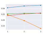
(a)

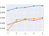
(b)

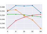
(c)

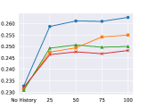
(d)

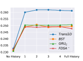
(e)

Figure 2. Parameter Sensitivity results. Y-axis represents $NDCG@5$, while similar trends are observed for all other metrics.

We next observe that, the context-aware baselines (i.e., ContextAware and LatentCross) perform similar to the average-pooling baselines. Here we note that, these baselines also perform average-pooling over the context-features (also referred to as the “next item features”). This supports our choice of adding the next possible item to the end of the sequence. Such a choice results in a similar effect to the context-aware approach that adds the item’s features as context not before the sequence (GRU) block is applied. Moreover, since we have a relatively small recall-set in our setting, it is possible to concatenate the predicted item features to the history sequence and leverage the Attention2D block to encode also the recall-set item attributes together with the sequence.

Finally, we can observe that, ordering by the RSP attribute results in a reasonable baseline on its own. This in comparison to both Price baselines that only provide a weak signal. This implies that, over our sampled users, the price does not pay a big deal, but rather the short-term interactions. This fact is further supported in our next parameter sensitivity analysis, see Figure 2(e).

4.4. Parameter Sensitivity

To better understand how the Trans2D model parameters influence its performance, we check its sensitivity to five essential parameters: 1) $L$, number of attention blocks, 2) $h$, number of heads used in the attention mechanism, 3) $d$, each attribute embedding size, 4) $N$, maximum sequence length, and 5) maximum number of days (back) to be considered in the sequence. For each parameter sensitivity check, we set the rest to their default values (i.e., $L=1$, $h=4$, $d=16$, $N=50$, and days=‘Full History’ – all days are being considered).

We report the sensitivity analysis results (using NDCG@5) in Figure 2. For reference, we also report the sensitivity of the three next best baselines: ${\textbf{GRU}}_{C}$, BST and ${\textbf{FDSA}}^{-}$. In general, we can observe that, in the majority of cases, our model outperforms the baselines. Furthermore, almost in all cases, the other baselines behave similarly to our model. Per parameter, we further make the following specific observations about our model’s sensitivity:

# Blocks ($L$): We notice that, adding a second Attention2D block on top of the first helps to learn second-order dependencies. This makes sense, as the two attention matrices of the model, $\mathbf{A}^{I}$ and $\mathbf{A}^{C}$, can capture attention only in the same row or column. The only attention type that can capture dependencies between two cells not in the same row or column is $\mathbf{A}^{F}$. Yet, during the attention calculation on $\mathbf{A}^{F}$, the cells are not aware of the other values in their row or column. Therefore, a second block is able to capture such second-order dependencies (e.g., price comparison of two different appearances of the same item or leaf-category). We can further observe that, the third block has less influence on performance. Finally, similar to the results reported in (Chen et al., 2019), with additional blocks, BST’s performance actually declines.

# Heads ($h$): Similar to normal attentions, utilizing more heads enables the attention mechanisms to learn multiple patterns. Here, we explore two main options for head sizes: 1) each head size equals the input size or 2) all head sizes together equal the input size. For our model and ${\textbf{FDSA}}^{-}$ the first option is better, while for BST, the second option is better. For the latter, this can be explained by its already over-sized input and data sparsity (see further details next in Embedding Size sensitivity). Overall, we observe that, $4$ heads resolves with a good performance, while $5$ heads already has a minor impact on our model’s performance.

Embedding Size ($d$): Interestingly, for our model, an embedding size of $d=32$ resolves with the best performance. While the trend for $d<32$ can be explained by too small representation sizes, the interesting trend is for $d>32$. This can be explained due the vocabulary size of each attribute. While most attributes include only few or tens of unique values, only user-ID, level1-category, and leaf-category hold $40,344$, $1,293$, and $25,449$ unique values, respectively. Therefore, while a larger representation may help the latter, the rest of the attributes suffer from over-representation and sparsity. We note that, those baselines that use concatenation (${\textbf{GRU}}_{C}$ and BST) can be thought as using a larger representation for each item. This fact supports the performance decline we observe for these baselines: with larger representations, more over-fit. Differently from the former two, ${\textbf{FDSA}}^{-}$ actually manages to improve (up to some point) with the increase in embedding size. We attribute this to its usage of the vanilla attention pooling over the attribute embeddings, which in turn, allows it to represent attributes together in an efficient way, even if some are very sparse.

Sequence Length ($N$) + Days Considered: The result of the RSP baseline implies that, users’ watchlist priorities are usually driven by short-term patterns. Such patterns are captured by users’ recently viewed item pages. We can observe that, for both parameters, $N=50$ or $days=1$ is enough in order to capture most of the important short-term signal. We further see a small improvement in extending the time range or sequence length. This implies that there is still a weak signal that can be captured. Since the sequence model is a Transformer, there is no memory-gate involved (like in GRU); hence, these short-term patterns represent a real user-behaviour.

4.5. Ablation Study

We next perform an ablation study and report the results in Table 2. To this end, every time, we remove a single component from the Trans2D model and measure the impact on its performance. We explore a diverse set of ablations, as follows:

$-{Linear2D}$: We switch every Linear2D layer with a Linear1D layer, meaning all channels receive the exact same weights. This ablation allows to better understand the importance of the attribute-alignment. While this modified component downgrades performance, it still outperforms all baselines while keeping the exact same number of parameters as in a regular attention layer (except for the three $\alpha$ scalars used in Eq. 2). This confirms that, the improvement of the full Trans2D results are not only driven by the Linear2D layer but also by the attention mechanism itself.

$-\mathbf{A}^{F}$,$-\mathbf{A}^{C}$,$-\mathbf{A}^{I}$: We remove each one of the three attention parts from the final attention calculation in Eq. 2. These ablations allow to better understand the importance of each attention type to the full model implementation. The most important attention part is $\mathbf{A}^{I}$, showing that the relationship between user’s items is the most important, following the motivation of the 1D-attention mechanism. $\mathbf{A}^{I}$ is followed by $\mathbf{A}^{C}$ and then by $\mathbf{A}^{F}$. As we can further observe, $\mathbf{A}^{F}$ does not hold significant importance. We hypothesis that, while $\mathbf{A}^{F}$ is the only attention part that can capture dependencies between two cells not in the same row or column, during the attention calculation on $\mathbf{A}^{F}$, the cells are not aware of the other values in their row or column. This can be over-passed by adding an additional Attention2D layer, as shown and discussed in Section 4.4 over the # Blocks sensitivity check, see again Figure 2(a).

$-RVI,-{watchlist}$: We remove from the history sequence all items having interaction type=RVI (item-page-view) and interaction type=watchlist (click), respectively. These ablations allow to understand the importance of each interaction type to the WLR task. While both are important, watchlist clicks hold a stronger signal. This actually makes sense: while item page views (RVIs) provide only implicit feedback about user’s potential interests, clicks provide explicit feedback that reflect actual user watchlist priorities.

Table 2. Ablation results. Starting from the second row, on each, a single component is removed from the model.

Model	Precision@k			HIT@k		NDCG@k
	@1	@2	@5	@2	@5	@2	@5
Trans2D (our model)	43.51	33.30	21.56	62.19	80.85	35.61	26.12
-$A^{F}$	44.01	33.42	21.56	62.42	80.85	35.82	26.20
-time	43.25	33.17	21.55	61.93	80.79	35.45	26.06
-RVI	43.21	33.09	21.51	61.81	80.62	35.38	26.01
-$A^{C}$	43.03	33.06	21.53	61.72	80.69	35.32	26.00
-item	42.21	32.64	21.40	60.89	80.13	34.80	25.74
-Linear2D	41.93	32.71	21.50	61.02	80.56	34.80	25.79
-watchlist	40.07	31.48	21.08	58.56	78.49	33.42	25.08
-$A^{I}$	38.83	31.60	21.36	58.84	79.92	33.24	25.14
-history	33.04	28.45	20.46	52.66	75.53	29.49	23.27
-position	32.18	26.77	19.86	49.45	72.81	27.99	22.51

$-time,-item,-position$: For each, we remove a group of attributes in order to better understand the importance of the attributes to the WLR task. For $-time$, we remove the hour, day, and weekday attributes. For $-item$, we remove the price, condition, level1-category, leaf-category, and sale-type attributes. For $-position$, we remove the position-ID, relative-snapshot-position (RSP), snapshot-ID, hash-item-ID, and hash-seller-ID attributes. Examining the ablations results, shows that the most important attribute-set is the position-set, followed by the item-set, and finally by the time-set. Noticing that the position-set includes RSP explains their high importance. The time-set is not that important as relative-time is encoded in the position-set. Additionally, the dataset spans over a relatively short period, resolving with less data to learn the importance of a specific weekday, hour of the day, or day of the month.

$-history$: To understand the importance of the entire history, we remove all the history sequence, and solely predict over $\mathbf{WL}_{t}$ – the last snapshot. We see that, not observing any history, drastically harms the performance of the model. This strengthens the argument that considering user’s history is important for the WLR task.

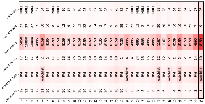
Figure 3. Qualitative Example. For brevity, only 6 out of the 16 possible attributes are presented. The darker the item-attribute cell color is, the more important it is. The current candidate is surrounded with the black rectangular.

4.6. Qualitative Example

We end this section with a qualitative example (see Figure 3) that visualizes the attention values assigned by the Trans2D model to items’ attributes in a given user-sequence. The last item in the sequence is the watchlist item for which the model makes a prediction. This item is actually clicked by the user ($y=1$) and the model’s prediction is aligned, assigning it the highest likelihood amongst all watchlist snapshot items ($\hat{y}=0.697$).

As the learned attention is a 4D-array, representing the attention between any two (item,attribute) pairs (see Section 3.5.2), we first pick the attention over the last item in the sequence, and then average over the channel dimension. Doing so, resolves us with a 2D-array that can be visualized to better understand the importance of each (item,attribute) pair on the prediction of the item. Observing the channel dimension, we can notice that, different attributes have different importance. This strengths the importance of a 2D-attention that is able to learn the attention over a second axis.

As we can observe, given the next item to predict, the model emphasizes either previously clicked items related to the current predicted item (e.g., leaf-categories: 8159–‘Home Security:Safes‘, 4895–‘Safety:Life Jackets & Preservers‘) or RVIs that belong to the same leaf-category of the current item (8159). Interestingly, the model emphasizes the prices of clicked items in the same leaf-category (8159), which are higher than the predicted item’s price.

5. Summary and Future Work

In this work, we presented a novel watchlist recommendation (WLR) task. The WLR task is a specialized sequential-recommendation task, which requires to consider a multitude of dynamic item attributes during both training and prediction. To handle this complex task, we proposed Trans2D – an extended Transformer model with a novel self-attention mechanism that is capable of attending on 2D-array data (item-attribute) inputs. Our empirical evaluation has clearly demonstrated the superiority of Trans2D. Trans2D allows to learn (and preserve) complex user preference patterns in a given sequence up to the prediction time.

Our work can be extended in two main directions. First, we wish to explore additional feedback sources such as historical user search-queries or purchases. Second, recognizing that Trans2D can be generally reused, we wish to evaluate it over other sequential recommendation tasks and domains.

References

- (1)
- Ba et al. (2016) Jimmy Lei Ba, Jamie Ryan Kiros, and Geoffrey E Hinton. 2016. Layer Normalization. stat 1050 (2016), 21.
- Beutel et al. (2018) Alex Beutel, Paul Covington, Sagar Jain, Can Xu, Jia Li, Vince Gatto, and Ed H. Chi. 2018. Latent Cross: Making Use of Context in Recurrent Recommender Systems. In Proceedings of the Eleventh ACM International Conference on Web Search and Data Mining (Marina Del Rey, CA, USA) (WSDM ’18). Association for Computing Machinery, New York, NY, USA, 46–54. https://doi.org/10.1145/3159652.3159727
- Chen et al. (2019) Qiwei Chen, Huan Zhao, Wei Li, Pipei Huang, and Wenwu Ou. 2019. Behavior Sequence Transformer for E-Commerce Recommendation in Alibaba. In Proceedings of the 1st International Workshop on Deep Learning Practice for High-Dimensional Sparse Data (Anchorage, Alaska) (DLP-KDD ’19). Association for Computing Machinery, New York, NY, USA, Article 12, 4 pages. https://doi.org/10.1145/3326937.3341261
- Chen et al. (2020) Tong Chen, Hongzhi Yin, Quoc Viet Hung Nguyen, Wen-Chih Peng, Xue Li, and Xiaofang Zhou. 2020. Sequence-aware factorization machines for temporal predictive analytics. In 2020 IEEE 36th International Conference on Data Engineering (ICDE). IEEE, 1405–1416.
- Eshel et al. (2021) Yotam Eshel, Or Levi, Haggai Roitman, and Alexander Nus. 2021. PreSizE: Predicting Size in E-Commerce using Transformers. arXiv:2105.01564 [cs.IR]
- He et al. (2016) Kaiming He, Xiangyu Zhang, Shaoqing Ren, and Jian Sun. 2016. Deep residual learning for image recognition. In Proceedings of the IEEE conference on computer vision and pattern recognition. 770–778.
- He et al. (2017) Ruining He, Wang-Cheng Kang, and Julian McAuley. 2017. Translation-Based Recommendation. In Proceedings of the Eleventh ACM Conference on Recommender Systems (Como, Italy) (RecSys ’17). Association for Computing Machinery, New York, NY, USA, 161–169. https://doi.org/10.1145/3109859.3109882
- Hidasi et al. (2016a) Balázs Hidasi, Alexandros Karatzoglou, Linas Baltrunas, and Domonkos Tikk. 2016a. Session-based Recommendations with Recurrent Neural Networks. arXiv:1511.06939 [cs.LG]
- Hidasi et al. (2016b) Balázs Hidasi, Massimo Quadrana, Alexandros Karatzoglou, and Domonkos Tikk. 2016b. Parallel Recurrent Neural Network Architectures for Feature-Rich Session-Based Recommendations. In Proceedings of the 10th ACM Conference on Recommender Systems (Boston, Massachusetts, USA) (RecSys ’16). Association for Computing Machinery, New York, NY, USA, 241–248. https://doi.org/10.1145/2959100.2959167
- Kang and McAuley (2018) Wang-Cheng Kang and Julian McAuley. 2018. Self-attentive sequential recommendation. In 2018 IEEE International Conference on Data Mining (ICDM). IEEE, 197–206.
- Kenton and Toutanova (2019) Jacob Devlin Ming-Wei Chang Kenton and Lee Kristina Toutanova. 2019. BERT: Pre-training of Deep Bidirectional Transformers for Language Understanding. In Proceedings of NAACL-HLT. 4171–4186.
- Kingma and Ba (2015) Diederik P Kingma and Jimmy Ba. 2015. Adam: A Method for Stochastic Optimization. In ICLR (Poster).
- Mizrachi and Levin (2019) Sarai Mizrachi and Pavel Levin. 2019. Combining Context Features in Sequence-Aware Recommender Systems.. In RecSys (Late-Breaking Results). 11–15.
- Pasricha and McAuley (2018) Rajiv Pasricha and Julian McAuley. 2018. Translation-based factorization machines for sequential recommendation. In Proceedings of the 12th ACM Conference on Recommender Systems. 63–71.
- Paszke et al. (2017) Adam Paszke, Sam Gross, Soumith Chintala, Gregory Chanan, Edward Yang, Zachary DeVito, Zeming Lin, Alban Desmaison, Luca Antiga, and Adam Lerer. 2017. Automatic differentiation in pytorch. (2017).
- Ren et al. (2020) Ruiyang Ren, Zhaoyang Liu, Yaliang Li, Wayne Xin Zhao, Hui Wang, Bolin Ding, and Ji-Rong Wen. 2020. Sequential Recommendation with Self-Attentive Multi-Adversarial Network. In Proceedings of the 43rd International ACM SIGIR Conference on Research and Development in Information Retrieval (Virtual Event, China) (SIGIR ’20). Association for Computing Machinery, New York, NY, USA, 89–98. https://doi.org/10.1145/3397271.3401111
- Rendle (2012) Steffen Rendle. 2012. Factorization Machines with LibFM. ACM Trans. Intell. Syst. Technol. 3, 3, Article 57 (May 2012), 22 pages. https://doi.org/10.1145/2168752.2168771
- Rendle et al. (2010) Steffen Rendle, Christoph Freudenthaler, and Lars Schmidt-Thieme. 2010. Factorizing Personalized Markov Chains for Next-Basket Recommendation. In Proceedings of the 19th International Conference on World Wide Web (Raleigh, North Carolina, USA) (WWW ’10). Association for Computing Machinery, New York, NY, USA, 811–820. https://doi.org/10.1145/1772690.1772773
- Sar Shalom et al. (2018) Oren Sar Shalom, Haggai Roitman, Amihood Amir, and Alexandros Karatzoglou. 2018. Collaborative filtering method for handling diverse and repetitive user-item interactions. In Proceedings of the 29th on Hypertext and Social Media. 43–51.
- Sar Shalom et al. (2017) Oren Sar Shalom, Haggai Roitman, Yishay Mansour, and Amir Amihood. 2017. A User Re-Modeling Approach to Item Recommendation Using Complex Usage Data. In Proceedings of the ACM SIGIR International Conference on Theory of Information Retrieval (Amsterdam, The Netherlands) (ICTIR ’17). Association for Computing Machinery, New York, NY, USA, 201–208. https://doi.org/10.1145/3121050.3121061
- Smirnova and Vasile (2017) Elena Smirnova and Flavian Vasile. 2017. Contextual sequence modeling for recommendation with recurrent neural networks. In Proceedings of the 2nd workshop on deep learning for recommender systems. 2–9.
- Sun et al. (2019) Fei Sun, Jun Liu, Jian Wu, Changhua Pei, Xiao Lin, Wenwu Ou, and Peng Jiang. 2019. BERT4Rec: Sequential recommendation with bidirectional encoder representations from transformer. In Proceedings of the 28th ACM international conference on information and knowledge management. 1441–1450.
- Tan et al. (2016) Yong Kiam Tan, Xinxing Xu, and Yong Liu. 2016. Improved Recurrent Neural Networks for Session-Based Recommendations. In Proceedings of the 1st Workshop on Deep Learning for Recommender Systems (Boston, MA, USA) (DLRS 2016). Association for Computing Machinery, New York, NY, USA, 17–22. https://doi.org/10.1145/2988450.2988452
- Tang and Wang (2018) Jiaxi Tang and Ke Wang. 2018. Personalized Top-N Sequential Recommendation via Convolutional Sequence Embedding. In Proceedings of the Eleventh ACM International Conference on Web Search and Data Mining (Marina Del Rey, CA, USA) (WSDM ’18). Association for Computing Machinery, New York, NY, USA, 565–573. https://doi.org/10.1145/3159652.3159656
- Tuan and Phuong (2017) Trinh Xuan Tuan and Tu Minh Phuong. 2017. 3D Convolutional Networks for Session-Based Recommendation with Content Features (RecSys ’17). Association for Computing Machinery, New York, NY, USA. https://doi.org/10.1145/3109859.3109900
- Vaswani et al. (2017) Ashish Vaswani, Noam Shazeer, Niki Parmar, Jakob Uszkoreit, Llion Jones, Aidan N Gomez, Lukasz Kaiser, and Illia Polosukhin. 2017. Attention is All you Need. In NIPS.
- Wang and Cai (2020) Baocheng Wang and Wentao Cai. 2020. Knowledge-enhanced graph neural networks for sequential recommendation. Information 11, 8 (2020), 388.
- Wang et al. (2019) Shoujin Wang, Liang Hu, Yan Wang, Longbing Cao, Quan Z Sheng, and Mehmet Orgun. 2019. Sequential recommender systems: challenges, progress and prospects. arXiv preprint arXiv:2001.04830 (2019).
- Wu et al. (2020) Liwei Wu, Shuqing Li, Cho-Jui Hsieh, and James Sharpnack. 2020. SSE-PT: Sequential Recommendation Via Personalized Transformer. In Fourteenth ACM Conference on Recommender Systems (Virtual Event, Brazil) (RecSys ’20). Association for Computing Machinery, New York, NY, USA, 328–337. https://doi.org/10.1145/3383313.3412258
- Zhang et al. (2019) Tingting Zhang, Pengpeng Zhao, Yanchi Liu, Victor S Sheng, Jiajie Xu, Deqing Wang, Guanfeng Liu, and Xiaofang Zhou. 2019. Feature-level Deeper Self-Attention Network for Sequential Recommendation.. In IJCAI. 4320–4326.
- Zhou et al. (2018) Chang Zhou, Jinze Bai, Junshuai Song, Xiaofei Liu, Zhengchao Zhao, Xiusi Chen, and Jun Gao. 2018. Atrank: An attention-based user behavior modeling framework for recommendation. In Proceedings of the AAAI Conference on Artificial Intelligence, Vol. 32.
- Zhou et al. (2020) Kun Zhou, Hui Wang, Wayne Xin Zhao, Yutao Zhu, Sirui Wang, Fuzheng Zhang, Zhongyuan Wang, and Ji-Rong Wen. 2020. S3-rec: Self-supervised learning for sequential recommendation with mutual information maximization. In Proceedings of the 29th ACM International Conference on Information & Knowledge Management. 1893–1902.