Analysis of core-mantle boundary seismic waves using full-waveform modelling and adjoint methods

Abstract

Using spectral-element synthetic seismograms and adjoint methods, we present a finite-frequency sensitivity analysis of traveltimes of seismic waves interacting with the core-mantle boundary (CMB). We focus on reflected and refracted P and S waves that are recorded in seismograms computed using SPECFEM3D_GLOBE. The core-mantle boundary is the most abrupt internal discontinuity of the Earth, marking the solid-fluid boundary between mantle and outer core that strongly affects the dynamics of the Earth’s interior. A lot of research has been dedicated to resolving the structure of the CMB interface, however, a high resolution image of topographic variations is still lacking, due to difficulties relating both to observations in seismograms and good understanding of lowermost mantle velocity structure. We select some of the most important and widely used seismic phases, namely ScS, SKS, SKKS, PcP, PKP, PKKP and PcS, given their path through mantle and core and their interactions with CMB. These seismic waves have been widely deployed by investigators, trying to comprehend CMB and lowermost mantle structure. Firstly, we use computed synthetic seismograms with a dominant period of T $\approx$11s for existing models of CMB topography and compare traveltime perturbations measured by cross-correlation to those predicted using ray theory. We find deviations from a perfect agreement between ray theoretical predictions of time shifts and those measured on synthetics with and without CMB topography. We find that these deviations are generally small when the background velocity model is 1-D, but become larger when a 3-D background model is used, indicating trade-offs between 3-D mantle structure and core-mantle boundary topography. Secondly, we calculate the Fréchet kernels of traveltimes with respect to shear and compressional wavespeeds and the boundary sensitivities with respect to the CMB interface. We observe that the overall sensitivity of the traveltimes is mostly due to volumetric velocity structure and that imprints of CMB on traveltimes are less pronounced. In general, higher frequency data is used for imaging CMB, but the intermediate frequency range used here is compatible with current computational capabilities and provides a first approach to an FWI modelling of deep Earth structure. Our study explains the difficulties relating to inferring CMB topography using traveltimes and provides a gallery of exact, finite-frequency sensitivity kernels. We conclude that imaging of CMB using full-waveform inversion (FWI) techniques and kernels as presented here can improve our understanding of deep Earth structure and trade-off between seismic velocities and boundary topography.

Keywords Core-mantle boundary, Global and Computational seismology, Finite-frequency kernels, adjoint methods, spectral-elements.

1 Introduction

The core-mantle boundary (CMB) is a major and sharp discontinuity inside the Earth, separating the mantle, composed of solid rocks, from the outer core, made of liquid iron alloy. Specifically, it lies between the mantle rocky aggregate and the liquid iron alloy outer core. Key phenomena affecting the Earth evolution and dynamics occur on each side of this boundary. For instance, on the mantle side, the CMB region is believed to be the source of mantle plumes, which trigger intraplate volcanism at the Earth’s surface. On the core side, magneto-hydrodynamic flow shapes magnetic field lines, partially controlling the magnetic field at the CMB.

The CMB is the location of interactions between the lower mantle and the outer core (e.g. Helffrich and Wood, 2001; Stevenson, 1981; Jeanloz and Williams, 1998; Gurnis et al., 1998; Lay et al., 1998). These interactions, in turn, influence mantle and core processes, for instance the geodynamo, and therefore the Earth’s magnetic field. Developments of consistent models of the mantle structure and dynamics above the boundary can improve geodynamo modelling, (e.g. Bloxham and Jackson, 1992). For instance, the heat flux at the CMB, imposed by mantle dynamics, influences the geodynamo, (e.g. Amit et al., 2015). Lateral variations of the core-mantle boundary radius, with its aspherical structure, may affect outer core flow processes, implying that a better image of CMB topography is essential to analyses of gravitational and topographical coupling between mantle and core, (e.g. Gubbins and Richards, 1986; Calkins et al., 2012; Davies et al., 2014).

From a seismological perspective, the core-mantle boundary is one of the most interesting regions for interdisciplinary geophysical research, however it is difficult to resolve it robustly. Over the years, much seismological research has been produced regarding lower-mantle and core-mantle boundary topography structure, using body waves and secondary phases of P and S waves, (e.g. Creager and Jordan, 1986; Doornbos and Hilton, 1989; Shen et al., 2016; Schlaphorst et al., 2016; Wu et al., 2014; Restivo and Helffrich, 2006; Sze and van der Hilst, 2003; Morelli and Dziewonski, 1987; Obayashi and Fukao, 1997; Rodgers and Wahr, 1993; Mancinelli and Shearer, 2016; Tanaka, 2010) as well as normal modes, (e.g. Ishii and Tromp, 1999; Xiang-Dong Li et al., 1991; Soldati et al., 2013). However, existing discrepancies among suggested CMB topography models for spherical harmonic degrees higher than two (Becker and Boschi, 2002; Koelemeijer, 2020) indicate that there may be features of the lowermost mantle structure, which need to be taken into account systematically. Additionally, possible inaccuracies in interpreting observed data can also be a reason for these differences, as most studies usually do not jointly explain CMB topography and velocity structure.

An important hindering factor is the complexity of the seismic structure in the bottom 300-400 km of the mantle. This includes the D" discontinuity, which is not present everywhere and is thought to be related to the phase transition from bridgmanite to post-perovskite, (e.g. Hirose et al., 2017; Cobden et al., 2015), ultra-low seismic velocity zones (ULVZ), which are thin pockets where compressional and shear wave velocities ($V_{P}$ and $V_{S}$) drop by up to 10 % and 30 %, respectively, (e.g. Yu and Garnero, 2018), strong, small-scale anomalies induced by cold oceanic slabs that have sunk down to the CMB, (e.g. Hung et al., 2005; Whittaker et al., 2015; Borgeaud et al., 2017), and the large low shear-wave velocity provinces (LLSVPs), defined as regions a few thousands of kilometers across where shear velocity drops by a few percent, and which are located beneath Africa and the Pacific ocean, (e.g. Li and Romanowicz, 1996; Ritsema et al., 2011; Lekic et al., 2012; Garnero et al., 2016; McNamara, 2018). Because they may be closely related to mantle dynamics, LLSVPs may strongly influence CMB topography. Numerical simulations showed that depending on their exact nature, clusters of purely thermal plumes or thermo-chemical piles, LLSVPs would trigger either uplifts or depressions in the CMB (Lassak et al., 2010; Deschamps et al., 2018).

Ideally, one would like to resolve CMB topography structure, while simultaneously obtaining an updated velocity model for the mantle. It has been shown by many researchers that CMB topography and mantle velocity variations exhibit strong trade-off, which makes the inference of a topographic map along the core-mantle boundary a hard task, (e.g. Garcia and Souriau, 2000; Sze and van der Hilst, 2003).

The nature of difficulties in resolving lowermost mantle structure can be analysed and addressed by investigating seismic waves which are sensitive to lowermost mantle structure and have been used to constrain the topography of the CMB. These seismic phases are characterised by complex wave phenomena occurring while travelling from the source to receivers, which makes it cumbersome to determine which type of seismic waves has a maximum CMB sensitivity. Nonetheless, there have been many studies analysing the compressional and shear wavespeed structure of the lowermost mantle using several related body wave phases as well as differential traveltimes between these, (e.g. Li and Romanowicz, 1996; Garnero, 2000; Garnero et al., 2016; Ritsema et al., 2011; Tanaka, 2002; Lekic et al., 2012; Muir and Tkalčić, 2020). A summary of the progress made during the last decades and relevant literature can be found found in (Gurnis et al., 1998; Garnero, 2000) and (Koelemeijer, 2020). In a different approach, studies (Colombi et al., 2012, 2014), based on axisymmetric spectral-element modelling (Nissen-Meyer et al., 2014), have implemented boundary and volume sensitivity kernels within a spectral-element code given spherically symmetric background models. They used this implementation to address the sensitivity of PcP and P_diff and showed a suite of sensitivity kernels to CMB structure (Colombi et al., 2012). Their research gave insights into how to incorporate sensitivity of traveltimes of P_diff, PKP, PcP and ScS for imaging the CMB (Colombi et al., 2014) in a joint inversion for boundary and lowermost mantle velocity structure in order to tackle the trade-off between parameters. Our study is stepping further by using the full-waveform synthetics calculated with spectral-elements in a cubed sphere, as implemented in SPECFEM3D_GLOBE, where the global wave propagation effects can be more accurately accounted for and implemented into the full-waveform processes in a consistent way.

The goal of this work is to investigate the finite-frequency sensitivity of frequently used seismic phases for lowermost and core-mantle boundary structure and provide a kernel gallery showing their sensitivity to boundary and volumetric isotropic structure. This is following the formulation of finite-frequency traveltime sensitivity given by (Marquering et al., 1999; Dahlen, 2005) and (Tromp et al., 2005) with the use of adjoint methods. The main contribution of this work is to better understand how to optimally use traveltime data of particular P- and S-waves for imaging the CMB and show how their sensitivities can be incorporated in a full-waveform inversion scheme that is targeted for resolving the lowermost mantle and CMB topography. We investigate a suite of P- and S-wave phases and their traveltimes as observed in synthetic seismograms computed for intermediate frequencies (0.01-0.08 Hz), which are at the higher end of frequencies used in global waveform inversion studies. We focus on the seismic phases PcP, PKP, PKKP, PcS, ScS, SKS and SKKS. We deploy a full-waveform, finite-frequency approach for analysing CMB related seismic waves, using well-established techniques based on spectral-element waveform modelling and adjoint methods for calculating the Fréchet sensitivity kernels, (e.g. Komatitsch and Tromp, 1999, 2002a, 2002b; Tromp et al., 2005).

To address the effects of adding topography and/or 3-D velocity variations on the traveltimes of these phases, we compare existing ray-based methods of inferring core-mantle boundary topography to cross-correlation time shift measurements made on the spectral-element synthetics. For this, we use full-waveform synthetic seismograms for events selected especially for CMB topography studies. The analysis is made by comparing traveltime anomalies predicted using ray theory, for the CMB topography models mentioned above, to residual traveltimes measured on full-waveform synthetics computed for the same CMB topography models. The traveltime comparisons are done similar to (Bai et al., 2012) and (Koroni and Trampert, 2016). This comparison could provide insights into the usability of the traveltimes of our selected phases within the ray theoretical framework. Using full-waveform modelling as realistic recordings, we can address the effects of varying the model on specific observables. This analysis should benefit from investigating the separate effects of 3-D mantle velocity structure and boundary topography on the traveltimes, when only these model parameters are perturbed during the simulations. The separate effects are examined by computing synthetics in a 3-D model and in a 1-D velocity model plus core-mantle topography. Our results show that for 1-D background the ray-theoretical framework works better for S phases than for P phases, while it deviates from a good prediction when the background velocity model is 3-D. We also find that the boundary sensitivity of almost all phases is much less pronounced than their clearer sensitivity to volumetric parameters, both compressional and shear velocity. This confirms the reported trade-off between CMB and 3-D velocity structure, and also indicates that all types of kernels shown here could be used to provide better constraints on relevant structures, as the CMB topography cannot solely be responsible for the traveltime shifts and the velocity structure imprint is significant.

The paper is structured as follows: We first present the methods for carrying out the traveltime analyses and comparisons. Then we explain the specifics of Fréchet sensitivity analysis. We present our results and we discuss them by addressing the effects of different CMB topography models, the influence of the background velocity model (1-D or 3-D). We also consider the different effects on P- and S- seismic phases. Finally, we explain the resulting Fréchet kernels in the context of full-waveform inversion and trade-off between the two parameters.

2 Methodology

2.1 Computation of synthetic seismograms

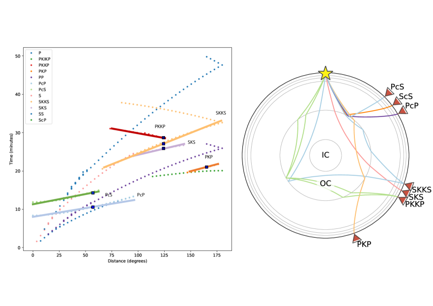
Figure 1: Left: Traveltime curves according to model PREM and tauP (Crotwell et al., 1999). The phases we investigate in this work are drawn with solid lines. More primary phases are plotted in order to justify the chosen epicentral distances for the sensitivity analysis. The characteristic distances chosen for computing the sensitivity kernels are shown by blue circles on the solid lines for each phase. Right: Theoretical raypaths for the same model. Red triangles denote stations at the epicentral distances were we opt observing the phases for the sensitivity analysis. The colours in the two sub-figures are not corresponding. IC denotes inner core, OC denotes outer core.

In order to enhance our knowledge about core-mantle boundary structure by investigating its effects on P- and S- seismic phases, we perform full-waveform modelling and focus on frequencies ranging from 0.01-0.08 Hz, given the computational limitations, still lying within an acceptable observational resolution. The theoretical raypaths of the chosen seismic phases are shown in Figure 1, which is produced using 1-D ray tracing with tauP (Crotwell et al., 1999) and using model PREM (Dziewoński and Anderson, 1981) as reference. The computation of synthetic waveforms is done using the community code SPECFEM3D_GLOBE (Komatitsch and Tromp, 2002a, b) in 1-D and 3-D mantle velocity models, namely PREM (Dziewoński and Anderson, 1981) and S20RTS (Ritsema and van Heijst, 2002), respectively. The synthetic waveforms are used to imitate realistic waveforms for the comparisons between ray theory and measurements and to assess the direct effects of CMB topography and 3-D velocity variations on the traveltime of the seismic phases.

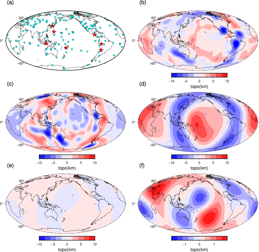
Figure 2: Maps of the earthquake events and stations used in this study (upper left). Maps of the CMB topography models used in this study are shown as well. Specifically, panel (a) shows the events (red stars) and stations from the Global Seismographic Network (cyan inverted triangles). Panels (b) to (e) show models T1 (b) and TC1 (c) based on the mantle convection simulations of (Deschamps et al., 2018) (see main text), and LM91 (Xiang-Dong Li et al., 1991) (d) and TK10 (Tanaka, 2010) (e), inferred from actual data. Panel (f) shows the same model TK10 as in panel (e), except for this time there is a change in scale of the colour bar, as this model’s topographic variations are much smaller than the other models.

For the comparisons of traveltimes derived using ray theoretical methods to measurements done on full-waveform synthetics, existing core-mantle boundary topography models are added, resulting in PREM or S20RTS plus CMB topography. A model with very low topographic variations is used, derived by (Tanaka, 2010) referred here as TK. In order to examine the effects of a variety of topographies with larger perturbations, we compute synthetic waveforms by also adding the models by (Xiang-Dong Li et al., 1991), denoted here as LM91, with peak-to-peak variation scaled up to 8 km, and two topography models derived from geodynamic simulations T1-pPv and TC1-pPv from (Deschamps et al., 2018), denoted here as T1 and TC1 for simplicity. In order to make the geodynamics models more applicable to our source-receiver geometry, model TC1 is rotated so that its spherical harmonic degree-2 pattern match best that of S20RTS S-velocity variations right above the CMB (this is done by performing a simple grid search). The same is done for model T1, but with the sign of S-velocity variations inverted. This is because S-velocity anomalies at the CMB, and CMB topography variations are expected to be positively correlated for thermo-chemical models (TC1), but negatively correlated for purely thermal models (T1) (Deschamps et al., 2018). These topography models are derived from purely thermal (T1) and thermochemical (TC1) simulations of mantle convection modelling. They were filtered for spherical harmonic degrees $\ell$ = 0 to $\ell$ = 20, and have absolute peak-to-peak amplitude around 20 km, for both models. Most of this amplitude is however accommodated by deep depressions caused by downwellings reaching the CMB, while positive topography associated with plume clusters in T1 and depressions associated with thermochemical piles in TC1 have height or depth, respectively, of about 2 km. Having various possible topography models allows us to investigate the reliability of ray theoretical methods in a more conclusive manner. All CMB topography models used here along with the dataset constructed by the earthquake events shown in table 1 are displayed in Figure 2.

For the simulations, we set the resolution such that the resulting noise-free waveforms have dominant period of about $T={11}$ s. Some modelling parameters which are present in real data can be important, such as attenuation, and can have complex effects on traveltimes of seismic phases, thus they are not considered for our simulations, since we want to focus on the effects of CMB topography and 3-D lateral isotropic variations without further complicating the waveforms.

To obtain a realistic dataset, we use seven events with a range of focal depths, source time function duration and moment magnitudes in the range $Mw=5.5-7.5$. The events are summarised in table 1. The receiver locations are set to those of the Global Seismographic Network and we make measurements for each source-receiver pair as well as ray theoretical predictions for the same pairs. This is done in time windows around the seismic phases of interest. The synthetic data are processed by filtering using a band-pass between the frequencies 0.01-0.08 Hz. The synthetic waveforms are used for two different purposes: Firstly, for comparisons of traveltime shifts caused by topographic variations in 1-D or 3-D mantle structure models and, secondly, for computing the sensitivity kernels for selected time windows encapsulating the maximum peak of the energy of our selected seismic phases.

GCMT ID	Event Location	Mw	Latitude (∘)	Longitude (∘)	Depth (km)	STF duration (s)
200609090413A	Flores Sea	6.3	-7.23	120.27	583.2	6.8
200707161417A	Sea of Japan	6.8	36.84	135.03	374.9	12.4
200709281338A	Volcano Islands (JP)	7.4	21.94	143.07	275.8	26.4
201409241116A	Jujuy Province (AR)	6.2	-23.78	-66.72	227.6	6.4
201303252302A	Guatemala	6.2	14.62	-90.71	186.4	6.2
200602021248A	Fiji Islands	5.9	-17.7	-178.13	611.6	11
101202H	Western Brazil	6.9	-8.30	-71.66	539.4	13.2

Table 1: Main features of the earthquake events used in this study. These are recorded at the station locations of the Global Seismographic Network.

2.2 Comparison of ray theoretical time shift prediction and cross-correlation measurements

In this section, we describe the prediction of traveltime anomalies due to perturbations of CMB topography using ray theory (RT), and as measured on full-waveform synthetics computed using the spectral element method (denoted by FW, which stands for full-waveform) using cross-correlation. The motivation of this analysis is to check whether we can reliably predict a topographic perturbation given the ray-theoretical framework. If this is true, the measured by cross-correlation time shift and the predicted time anomaly for a specific topographic variation should be identical. In the opposite case, where the two values diverge, there are two implications: firstly, the ray-theoretical framework is not sufficient for translating the time shift measured to topographic variation; secondly, there are velocity effects which are not adequately taken into account when using a linearised inversion. Traveltime perturbations due to the CMB topography are computed in the framework of ray theory following (Morelli and Dziewonski, 1987; Tanaka, 2010), using the expressions given in eq. 1 when the ray reflects off the CMB (e.g., ScS), and eq. 2 when the ray transmits through the CMB (e.g., SKS):

$$\delta t_{ref}=-\frac{2}{r}\left(\eta^{2}-p^{2}\right)^{\frac{1}{2}}\delta r,$$ (1)

$$\delta t_{tra}=-\frac{1}{r}\left[\left(\eta_{+}^{2}-p^{2}\right)^{\frac{1}{2}}-\left(\eta_{-}^{2}-p^{2}\right)^{\frac{1}{2}}\right]\delta r,$$ (2)

where $\delta r$ (in km) denotes the variation of the CMB radius at the bouncing points, $p$ (in s/rad) is the ray parameter for the 1-D model without perturbations of CMB topography, and $\eta=r_{cmb}/v(r_{CMB})$ (in s/rad) is the vertical ray parameter, with $\eta_{+}$, and $\eta_{-}$ representing the values of $\eta$ just above, and below the CMB, respectively. For PREM, which is our selected model, $\eta_{+}=479.03$ for S phases, and $\eta_{+}=253.71$ for P phases, while $\eta_{-}=431.51$ (only P phases are supported in the core).

Traveltime perturbations for the synthetics are computed by cross-correlation between synthetics for the reference model (either PREM, or S20RTS) and for the same model with added perturbations of CMB topography. For each of the seismic phases ScS, SKS, SKKS, PcP, PKP, PKKP and PcS, we first compute preliminary time windows from 5 s before, to 20 s after the arrival time of the phase as predicted using tauP (Crotwell et al., 1999) and PREM. We exclude time windows that overlap with the phases S, SS, SSS, sS, P, pP, PP, PPP, sP and pS, since overlapping phases affect the traveltime measurement by cross-correlation, which makes the comparison with ray theory less meaningful.

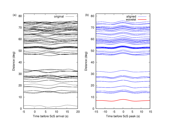
Figure 4: Illustration of the adaptive stacking procedure (Rawlinson and Kennett, 2004) used to define the time windows, for the ScS phase for model S20RTS and event no. 1 in Table 1. (a) Waveforms before alignment, using time windows 5 s before, and 20 s after the ScS arrival; (b) same as (a), but after alignment using the source wavelet (red trace) obtained from the adaptive stacking procedure.

For a given reference model, we then compute improved time windows centered on the peak of each phase following the adaptive stacking algorithm of (Rawlinson and Kennett, 2004), in order to: 1) correct for the shift in travel-time for the case of a 3-D reference model, and 2) further eliminate time windows with overlapping phases. The improved time windows have a length that ranges from -15 s to +15 s after the arrival time of the peak for each phase. The output of the adaptive stacking algorithm is the time windows aligned on their respective peak amplitude and an average source wavelet that represents the apparent source time function of the phase of interest. An example of the adaptive stacking procedure is shown in Figure 4. The selection of time windows without overlapping phases is done by imposing a minimum cross-correlation coefficient between a given time window, and the inferred source wavelet. In the remaining of this section, the minimum cross-correlation coefficient is set to 0.8 for the P phases (PcP, PKP, PKKP and PcS), and to 0.95 for the S phases (ScS, SKS, SKKS), due to the higher signal-to-noise ratio for S- than for P-waves. For the PcP phase, we further exclude all records at epicentral distances smaller than 40^∘, since such records show consistent, large disagreement between RT and FW. The total number of time windows before and after selection is shown in Table 2. The amount of time windows that pass our quality criteria becomes significantly smaller, however, we prefer to base our conclusion on a more robust dataset. The smaller numbers of high correlation coefficients time windows in noise-free synthetics also shows that the isolation of these phases can be considerably cumbersome in real datasets.

Phase	Before selection	Selected (PREM)	Selected (S20RTS)
ScS	1273	795	550
SKS	2262	932	905
SKKS	2296	587	666
PcP	570	137	151
PKP	375	322	264
PKKP	1715	700	775
PcS	889	449	379

Table 2: Number of time windows used in this study, for each phase before selection based on cross-correlation coefficients, and after selection for the PREM and S20RTS models. Note the smaller number of PcP time windows before selection compared to ScS, which is in part due to P merging with PcP at smaller epicentral distances than for S and ScS.

2.3 Computation of Fréchet sensitivity kernels

The sensitivity kernels are computed for time windows of 30 s length, centered on the predicted peak arrival of the P- and S-wave phases under investigation. The sensitivity is computed based on the Born approximation (e.g. Marquering et al., 1999; Dahlen et al., 2000; Dahlen, 2005) and using adjoint methods as implemented in the software package SPECFEM3D_GLOBE for boundary (Dahlen, 2005; Liu and Tromp, 2008) and volumetric kernels (Tromp et al., 2005). With this analysis, we conduct an investigation of the traveltimes by visualising their sensitivity to volumetric, namely shear and compressional velocity mantle structure, and boundary parameters, this is interface denoting CMB. The main goal is to distinguish these phases which can truly help us to improve core-mantle boundary topography models in a full-waveform inversion scheme, judging by the effect this has on their traveltime.

More specifically, the kernels are computed with respect to the CMB radius and compressional and shear wavespeed in 1-D background model PREM. We compute the so-called "banana-doughnut" traveltime kernels , (e.g. Luo and Schuster, 1991; Marquering et al., 1999; Dahlen et al., 2000), which associate a traveltime measurement on the waveforms to the changes in the finite-frequency sensitivity depending on the background model. The traveltime refers to the time window around the arrival of the phase according to a given model, which we have fixed to PREM, for a single pair of source-receiver. The relationship connecting a traveltime window to volumetric structure defined by seismic properties of compressional ($\alpha$) and shear ($\beta$) wavespeed are shown below. The following expressions are given for a reference seismic receiver ($r$) at position $x_{r}$. The reader is referred to (Tromp et al., 2005) for the complete derivations according to the Born approximation and the adjoint method. The volumetric kernels are related to the time window via:

$$\delta T_{r}=\int_{V}K_{\alpha,\beta}(\mathbf{x},\mathbf{x_{r}})\delta\ln\alpha,\beta(\mathbf{x})d^{3}\mathbf{x},$$ (3)

The units of volumetric wavespeed kernels are $s\cdot km^{-3}$.

The expression relating the traveltime window which encloses the seismic phase to the boundary perturbation on the core-mantle boundary (solid-fluid interface denoted by $\Sigma F$) is based on theory derived by (Dahlen, 2005) and implemented in the spectral-element method:

$$\delta T_{r}=\int_{\Sigma F}\mathbf{K}_{h}\cdot\delta h(\mathbf{x})d^{2}\mathbf{x},$$ (4)

whereby $\mathbf{{K}_{h}}$ is the time integration for variations along the boundary (Dahlen, 2005). The units of boundary kernels are $s\cdot km^{-2}$.

We select the phases for an ideal set-up of source-receiver given their epicentral distance also according to literature and optimal theoretical observational range. Specifically, for phases ScS, PcP, and PcS the epicentral distance is chosen to be 53^∘, as at this distance they are less likely to interact with SS, PP, and P, respectively. The phases PKKP, SKS, and SKKS are observed at an epicentral distance equal to 110^∘ for better isolation of their theoretical arrival time. The PKP phase is selected at a distance of 160^∘ as, according to 1-D ray theory and tauP analysis, at this distance, it is better separated from PKIKP. The phases that travel through the outer core as well as PcS are time windowed on radial components of the synthetic seismograms, as they are expected to have maximum energy at this component, while core reflected phases are observed and analysed on the vertical (for PcP) and transverse component (for ScS). The traveltime curves are shown in figure 1 with annotated characteristic distances for each seismic phase window.

For the visualisation of the sensitivity kernels, we use a characteristic scale length, which is appropriate for the range of data values of the kernels and allows us to observe the theoretical finite-frequency sensitivity. It is helpful to consider that the volumetric and boundary kernels have different units and are explicitly calculated for different parameters; therefore the model update using these kernels will be different in the context of full-waveform inversion, depending also on the optimisation algorithm chosen for the potential model updates. Considering the expression given above, i.e. eq. 3 and eq. 4, it is not easy to directly compare boundary to volumetric kernels and assess how they will change the initial model. It is however meaningful to consider that the traveltimes of the selected seismic phases will likely show sensitivity to both parameters, as expected by the potential trade-off between velocity and CMB structure, and thus it is worthwhile to judge the qualitative effects of volumetric and boundary structure separately.

3 TRAVELTIME ANALYSIS USING FULL-WAVEFORM MODELLING

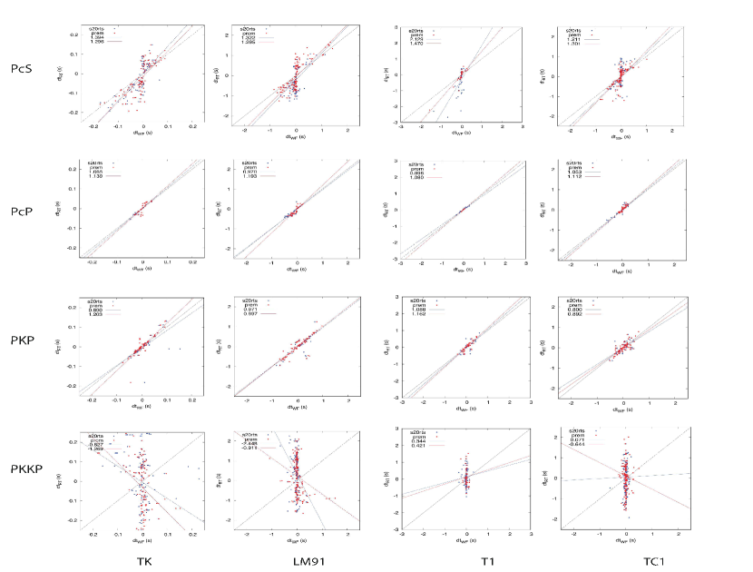
Figure 5: Comparison between ray theoretical prediction of time shift given a CMB topography model to the time anomaly measured on each time windowed seismic phase by comparing synthetic waveforms in 1-D and 3-D velocity background, red and blue points on the plots, respectively. Each column corresponds to a different topography model (TK, LM91, T1, TC1). Each row corresponds to a seismic phase (PcS, PcP, PKP and PKKP). Most of the phases show acceptable correspondence between predicted and measured by cross-correlation time shift, implying that the signature of CMB topography can be only partially captured by using RT. This is not the case for phase PKKP, where a prediction fails completely and the time window isolation is insufficient to make a reliable measurement.

In this section, we show the comparisons of traveltime anomalies measured on FW synthetics to RT prediction for phases ScS, SKS, SKKS, PcP, PKP, PKKP, and PcS. In Figures 5 and 6, we present the results of this comparison for all topography models and for all the selected phases, for synthetic waveforms calculated using PREM, and S20RTS (1-D, and 3-D, respectively) as velocity background model. Figures 5 and 6 show that there is part of the measured traveltime shift which is not fully recovered when translating a topographic variation to time delay using ray theory. This essentially means that the ray theoretical expression cannot fully explain the topographic variation as time anomaly measured in full-waveforms with and without topography perturbation. The discrepancy seems to increase linearly with $dt_{RT}$, and thus with the amplitude of the CMB topography, and varies significantly for different topographic models and phases. If the recovery using RT could accurately explain the traveltime shifts on these seismic phases, all points in Figures 5 and 6 would lie on the line with slope equal to one. However, the slopes of the linear regression lines have values different from one, as shown in Table 3. For the ScS phase (which gives the most corresponding results between RT predictions and WF measurements) with PREM as a background model, deviations from a perfect agreement are between 2% to 7%, while other well-resolved phases (SKS, SKKS, PcP and PKP) show deviations of up to 26% (for the SKS phase for model T1). This is true when the background velocity model is identical between the compared waveforms, namely with and without the topography model. In this case, we use PREM which is a 1-D model and is also consistent with the ray theoretical predictions made for the given topography model.

Figures 5 and 6 show that the agreement between a ray theoretical prediction of time anomaly caused by topography and the equivalent measurement on full-waveform synthetics is better for S-wave phases than for P-wave phases. More specifically, ScS, SKS, SKKS (and PKP from the P-waves) traveltime shifts due to topography seem to be better predictable with ray theory. However, it should be noted that the difficulty in predicting an adequate time anomaly may not be solely due to ray theoretical limitations. Additional difficulties may also arise when trying to isolate the P-waves.

Focusing now on the comparisons of ray theoretical predictions to measurements on full-waveforms using S20RTS as a background model (blue dots on Figures 5 and 6), we see that the agreement between RT and WF is worse than when using PREM as a background model. Table 3 summarises the slope values, for example, for the ScS phase, deviations from a perfect agreement between RT and WF are $\sim$1.6 to $\sim$3.5 times larger (i.e., 5% to 18%) for S20RTS as a background model than for PREM, depending on the topographic model. The slopes vary significantly with the topographic model, and seem to be larger for models with bigger absolute topographic variation or smaller-scale amplitudes of CMB topography.

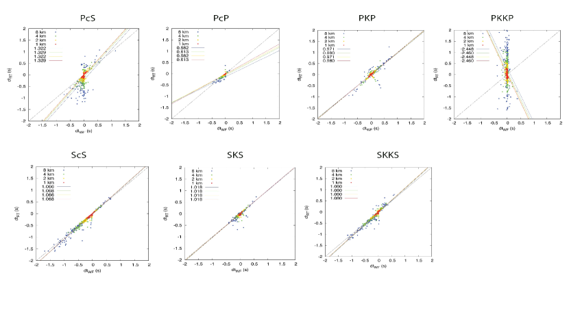
Figure 7: A test using four version of the same topography model to check whether the amplitude of the variation linearly affects the RT prediction and cross-correlation time shift measurements. The model LM91 is scaled for $\pm$1 km (yellow dots), $\pm$2 km (orange dots), $\pm$4 km (green dots) and $\pm$8 km (blue dots) topographic variations. The slopes of a simple linear regression for the cloud of points remain almost unchanged with the scaling of the model. This indicates that there is no clear dependence on the topographic variation when considering the agreement between prediction of RT and CC measurement.

We further investigated this behaviour by computing traveltime residuals for three scaled versions of model LM91, with maximum topographic amplitudes of $\pm$1 km, $\pm$2 km, and $\pm$4 km, in addition to the original LM91 model, whose maximum amplitude is $\pm$8 km. These are shown in Figure 7. The results for the case of a 3-D background model show that the slope values are very close for all the scaled versions and the original model. This implies that the amplitude of the topography has some effect, but that it does not crucially affect the agreement between RT and WF, at least for amplitudes up to $\pm$8 km. The differences in slopes for different topographic models could therefore be due to differences in the scale of the topographic anomalies. We note that S20RTS is a relatively smooth 3-D model compared to more recent global tomographic models. We expect even larger discrepancies for 3-D models with stronger, smaller-scale velocity anomalies (e.g., S40RTS (Ritsema et al., 2011) or SEMUCB-WM1 (French and Romanowicz, 2014)).

Our results illustrate the key role played by 3-D velocity variations in determining traveltimes. While ray theoretical predictions are based on a 1-D ray tracing expression, the result remains that the measurements on full-waveform synthetics show discrepancies with predictions, even though the measurement is done by comparing 3D and 3D+CMBtopo synthetics (keeping a fixed velocity model), indicating a non-linear effect of the two parameters to the traveltime. This also shows the highly non-linear effects of topography and 3-D variations on traveltimes of these phases, when topography is the only parameter added to the simulation. It is expected that some of the mismatch could properly be accounted for when a 3-D velocity correction is made, but it is not expected that it will fully be compensated, due to non-linear trade-off between CMB topography and the 3-D structure of the lowermost mantle, and to finite-frequency effects discussed in the next section.

Phase	T1	TC1	TK10	LM91
phase	T1	TC1	TK10	LM91
ScS	1.18/1.07	1.08/1.05	1.05/1.02	1.07/1.02
SKS	0.88/0.79	1.09/0.79	0.26/0.87	1.02/0.97
SKKS	1.14/1.16	1.03/1.17	0.96/1.19	1.08/1.11
PcP	0.90/1.08	1.05/1.11	1.06/1.14	0.97/1.19
PKP	1.09/1.16	0.80/0.89	0.89/1.20	0.97/1.00
PKKP	0.34/0.42	0.07/-0.64	-0.83/-1.27	-2.45/-0.91
PcS	2.13/1.47	1.21/1.30	1.39/1.30	1.32/1.29

Table 3: Slopes of the linear regression lines for the $dt_{RT}$ vs. $dt_{WF}$ diagrams in Figures. 5 and 6. Each cell shows two slopes, which correspond to S20RTS (left side of the forward slash), and PREM (right side) as a background model, respectively.

4 FRÉCHET KERNEL GALLERY FOR CORE-MANTLE BOUNDARY RELATED PHASES

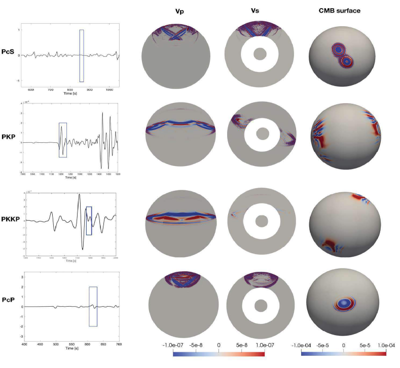
Figure 8: Fréchet sensitivity kernels for the group of P-waves examined here. Each row corresponds to a phase, from left to right, the figures show: synthetic seismogram and corresponding time window isolating the phase, compressional wavespeed volumetric kernel ($V_{P}$), shear wavespeed volumetric kernel ($V_{S}$), boundary kernel on denoting the core-mantle transition. From top to bottom: PcS (53^∘), PKP (160^∘), PKKP (110^∘), PcP (53^∘). The units of volumetric kernels are $km^{-3}\cdot s$ and for the boundary kernels $km^{-2}\cdot s$.

Figure 8 shows the complete sensitivity of the P-wave phases under investigation. The Fréchet derivatives are computed for compressional ($V_{P}$) and shear wavespeed ($V_{S}$) as well as for boundary of the interface corresponding to core-mantle boundary at approximately 2890 km for the chosen background model, PREM. All P-wave phases show their theoretical, finite-frequency, hence broader Fresnel zone, sensitivity to $V_{P}$. This indicates that the time window chosen around the predicted arrival according to PREM encapsulates the phases well enough and they present little or no interference with other waves. It is worth noting that, specifically for the PcS and PcP phases, they seem to exhibit considerable sensitivity to shear wavespeed as well, showing the more complex contributions to their traveltimes and perhaps explaining the weakening of their sensitivity to topography, as shown in the analysis done in section 3.

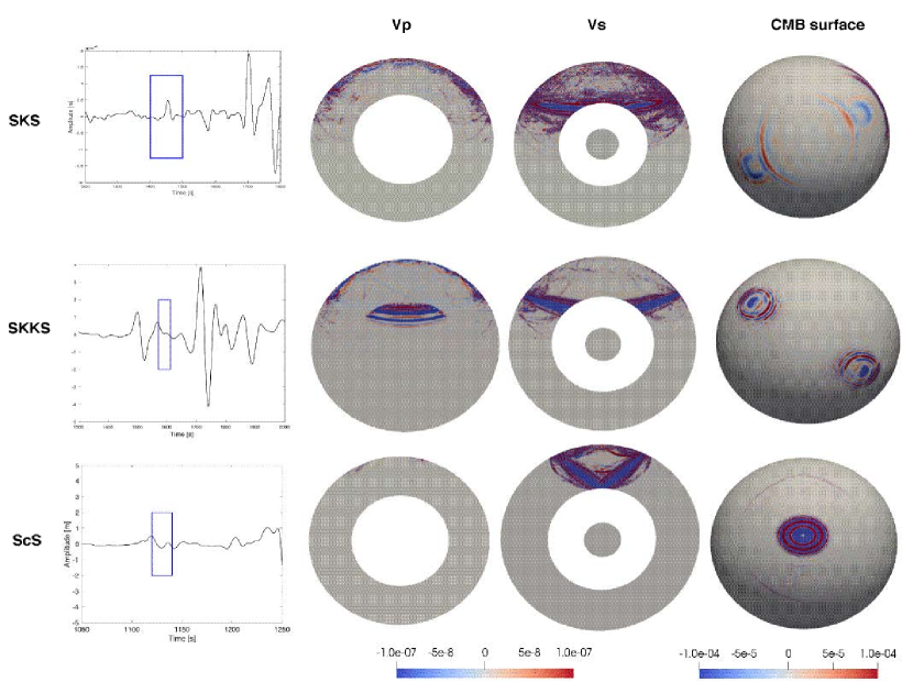
Figure 9: Similar to figure 8, now for the selected S-wave phases. From top to bottom: SKS (110^∘), SKKS (110^∘) and ScS (53^∘). The units of volumetric kernels are $km^{-3}\cdot s$ and for the boundary kernels $km^{-2}\cdot s$.

Regarding the S-wave phases, displayed in Figure 9, their traveltime sensitivity to shear and compressional wavespeeds and CMB surface are shown in a similar way as in Figure 8. It is readily observed that the shear wavespeed kernels computed for the time windows around the predicted arrival of these phases also clearly show their theoretical path, in this case broader and more extended due to the finite frequency effects which are in this case properly accounted for. The seismic phase SKS shows a broad and noisy sensitivity. The travelling paths of SKS, SKKS through the mantle are very similar, with their major differences appearing within the outer core. This is why their differential time has frequently been used for shear wave splitting studies in the lowermost mantle, (e.g. Restivo and Helffrich, 2006; Favier and Chevrot, 2003; Sieminski et al., 2008; Souriau and Poupinet, 1991). In the context of our study, it is important to understand their finite-frequency sensitivity and its variability between the two phases when it comes to the CMB surface. The S-wave phases also show clear contributions only from their theoretically predicted path in the time window selected for the calculation. In contrast to the P-wave kernels, there is little to none sensitivity of these phases to compressional wavespeed.

Turning to the boundary kernels, from visual inspection it becomes apparent that contributions to the traveltime sensitivity are low, especially for the traveltime windows of PKP and PKKP. This is in reference to the background model PREM. A low sensitivity to that means that the theoretical traveltime has low values at the interface of the core-mantle boundary, hence the particular seismic phase does not seem to arrive at a considerably different time than that reference traveltime prediction using PREM, due to the interaction with the core-mantle boundary and its topography. The boundary sensitivity of PcS and PcP are more pronounced and seem to sample its structure adequately and with the typical top-side reflection Fresnel zone. Considering the boundary sensitivity of S-waves, from the kernels in Figure 9, we observe that also for these phases, the reflected ScS phase has a clear sensitivity to the CMB. However, for SKS and SKKS, as shown by their corresponding boundary kernels, most of the sensitivity is observed at the piercing points in and out their way to the core, with SKKS having a stronger contribution. We discuss these results in greater detail in the next section.

5 DISCUSSION & CONCLUDING REMARKS

We have presented a traveltime analysis, where a ray theoretical prediction of traveltime anomaly caused by core-mantle boundary topography variations was compared to a measurement made by cross-correlation on full-waveform synthetics, imitating the common techniques of measuring time shifts on recorded waveforms to infer CMB topography. The retrieval of traveltime anomalies using ray theory shows that we could predict the shift caused by a given topography variation, albeit with some loss of accuracy and most reliably in time windows for the selected S-wave phases. We also showed that the correspondence worsens when the measurements are made in a 3-D background model, implying considerable effects of lateral velocity variations on the traveltimes. This is shown by a deviation from a perfect linear correspondence between the prediction and the measurement on realistic waveforms.

For the P-wave phases, the correspondence between ray theory and measurements on waveforms is much worse than for S-wave phases, except for PKP and PcP. The lack of agreement could be associated with better time window isolation of the given S-wave phases, contrary to the difficulties occurring for P waves. Specifically, multiple branches of PKKP can make its peak separation from its different branches (e.g. PKKPdf) more difficult than for other phases. It is also generally expected that P-wave propagation is more complex when interaction with strong velocity contrasts occurs (Aki and Richards, 1980; Doornbos and Mondt, 1980). This involves both up- and down- going P and S waves when a P-wave interacts with an interface, and especially the CMB, due to the strong contrasts in density and thermo-elastic properties between the solid rocks defining the mantle and the liquid iron alloy determining outer core composition.

For both the case of PREM (Figures 5 and 6 red points) and S20RTS (Figures 5 and 6 blue points) as a background model, we observe deviations from a perfect agreement between traveltime residuals predicted by ray theory, and those measured using cross-correlation on realistic waveforms (slope value equal to unity). The deviations seem to increase linearly with the amplitude of the CMB topography. The rate of increase does not seem to depend on the amplitude of the CMB topography, but varies with topographic models, which could indicate a dependence on the scale of topographic anomalies. In particular, the rate seems larger for CMB topography models T1 and TC1 (Deschamps et al., 2018), which have smaller-scale anomalies, but are not built on seismic data and whose geographical distribution may thus differ significantly from the real CMB topography. The deviations for the case of PREM as a background model are between 2% to 7% for the ScS phase (the phase with the most reliable measurements), and between 5% and 18% for the case of S20RTS as a background model.

The slopes given in Table 3 for each of the phases and each of the background model show that the sign of the topographic variation can be in most cases correctly defined. However, for the PKKP phase and all models tested in our study, the measurement done in both background models seems to fail to infer the correct sign of topography (negative slopes). The linear regression attempted to fit the points of measurement, though, is not efficient as there are many points for which the ray theoretical prediction is close to zero. This perhaps implies that PKKP is indeed difficult to isolate and given its multiple branches, an assignment to its traveltime shift due to CMB topography, neglecting effects from lowermost mantle and outer core velocity variations, is a rather simplified assumption as many effects can lead to almost synchronous arrivals (e.g. Earle and Shearer, 1997; Rost and Revenaugh, 2003). We note that difficulties isolating separate branches of the PKKP phase would be reduced when using higher-frequency waveforms, as usually done when using ray theory, (e.g. Tanaka, 2010). This is, however, not currently possible when using our spectral-element synthetics, because of the significant increase in computational requirements for higher frequencies. This implies that phases such as high-frequency PKKP are currently difficult to use in full-waveform inversion for the core-mantle boundary topography.

The smaller deviations when using PREM as a background model suggest that the ray theory expressions in eqs. 1 and 2 are not completely adequate for the time shift measurements on 3-D background. These are derived using the ray parameter for a 1-D model (i.e., without topography), which implies that the observed deviations could be an effect of the small change in ray parameter due to the addition of CMB topography. Most likely though, the deviation could be due to finite-frequency effects when using the full-waveform theory. The larger deviations observed when using S20RTS as a background model indicate trade-offs between the CMB topography, and 3-D S- and P- velocity anomalies in the mantle. For model T1 with strong, small-scale topographic anomalies beneath cold downwellings at the CMB, the deviations reach 18% for the ScS phase. This could affect the accuracy of inferred global tomographic models, which often do not account for the core-mantle boundary topography, although deviations in our calculations are not so large as to imply significant artifacts in tomographic models.

The finite-frequency sensitivity kernels show that the phases we investigated have strong contribution in their predicted traveltime windows and are not interfering with other phases. This observation shows that measurements on these phases can contribute to a good quality traveltime dataset and misfit measurements on their time windows and could help for a meaningful model update, given that they can be well separated with time windows. We also observe that reflected P-wave phases, i.e. PcP and PcS, are sensitive to shear wavespeed structure, too. In common inversion methods for imaging CMB topography, traveltimes are corrected for mantle velocity structure. The traveltime sensitivity of the S-waves does not seem to present similar patterns to that of P-waves, namely the traveltime is affected almost only from shear wavespeed variations. This may partly explain the poorer agreement between ray theory and measured traveltimes for P-waves than for S-waves, as the ray theoretical prediction does not account for the influence of shear wavespeed structure on the P-wave traveltimes (for example see expression 1). It also implies that linearised corrections for mantle structure may require the correction for shear wavespeed structure as well, similar to a conclusion made by (Koroni et al., 2019) for the, rather difficult to observe, PP precursors.

The sensitivity of the traveltimes to CMB seems to be weak for most of the selected time windows, implying that the contribution of the CMB interface to the traveltime shift is too weak to provide a robust update of the topography. Notable exceptions are the phases which reflect off the CMB, namely the ScS, PcP, PcS and to a lesser extent SKS, SKKS at the piercing points on the way in and out the outer core. This indicates that for purely CMB topography retrieval using traveltimes of these phases, one should consider that their sensitivity differs significantly and some phases offer a more optimal illumination of CMB structure than others (for example compare ScS to SKS).

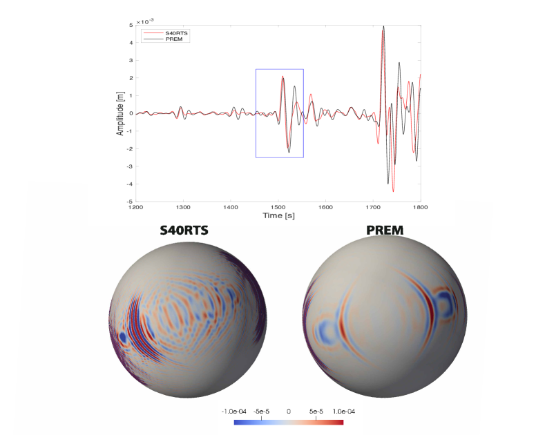
Figure 10: Comparison between the boundary kernels computed in 3-D background using model S40RTS (red line) and the same seismic phase SKS in 1-D background PREM (black line). the fact that the boundary kernels differ due to the different background model shows that interpretation of the traveltime shift of the phases due to topography should take into account the trade-off between topography and 3-D velocity variation, ideally in a non-linear way (not only by subtracting a time shift correction due to the 3-D mantle model). The units of boundary kernels $km^{-2}\cdot s$.

Trying to explain the discrepancies between predicted and measured traveltime anomaly when working in 3-D background, this time in PREM and S40RTS (Ritsema et al., 2011) (1-D and 3-D mantle models), we computed boundary sensitivity kernels for the same time window isolating the phase SKS, same station-source configuration as in Figure 6. This phase is chosen for exemplification. The resulting kernels show that the 3-D model in the background significantly affects the boundary sensitivity of the traveltime, see Figure 10. This indicates that 3-D effects are imprinted into the traveltime of seismic phases and their sensitivity to the CMB is clearly changing in a substantial way, thus making an interpretation of the traveltime anomaly due to only topographic variations difficult. Additionally, given that our knowledge for the lowermost mantle structure is still lacking sufficient resolution, a joint inversion using Fréchet kernels, where both velocity and CMB topography are updated, may be more appropriate for the nature of this problem. This also confirms the traveltime analysis comparing traveltimes calculated using ray theory to those measured on synthetics, and indicates that not addressing this trade-off could bias both the resulting velocity structure and the inferred CMB topography.

From our sensitivity analysis we can conclude that top reflected seismic phases (e.g. ScS) are adequately informative for properly imaging CMB topography using boundary kernels. We also find that the effect of the velocity variations are significant and should be taken into account using the volumetric finite-frequency kernels as shown in this work. To reliably separate the two effects seems complicated, especially with an one step approach; however, it can be more efficient to utilise an iterative optimisation of a starting model and help make better inferences about CMB topography. High resolution imaging of the CMB and the mantle structure just above this interface requires an interdisciplinary approach. Understanding how subduction processes and hot material accumulated at the bottom of the mantle can affect observations of seismic phases traveltimes on the recordings is fundamental for a clarified selection of seismic traveltime data with stronger sensitivity at these regions.

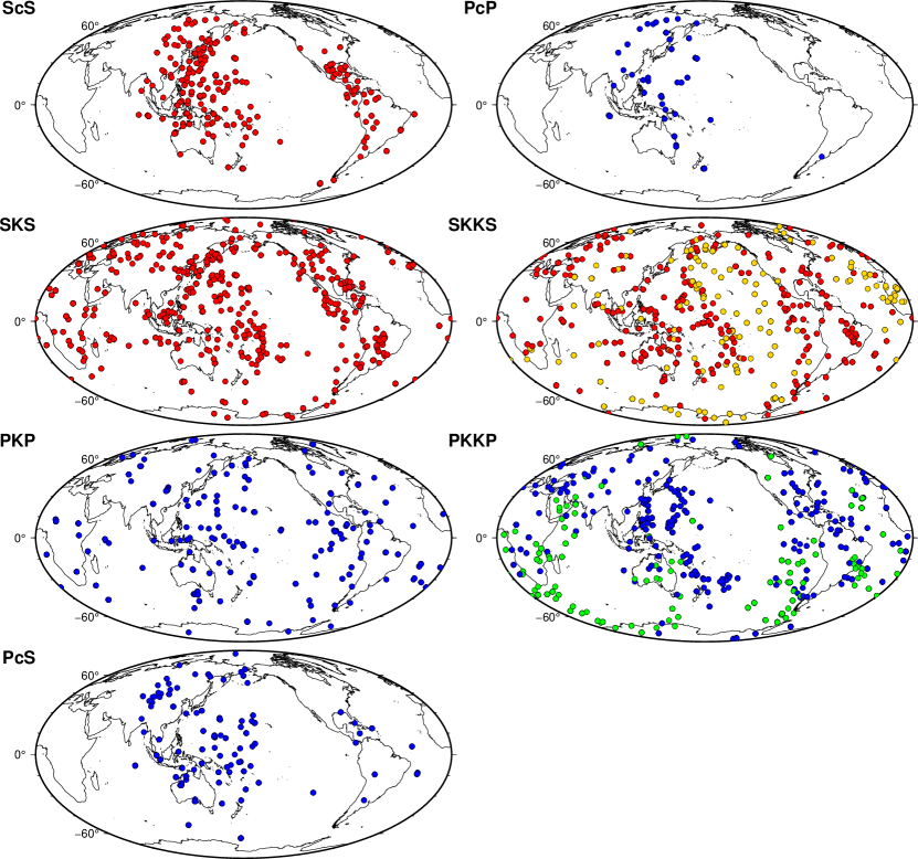
Figure 3: Bouncing or crossing points at the CMB for the seven seismic phases used in this study, as labeled in each panel. Blue-filled circles show P phases, while red circles show S phases. For SKKS and PKKP, yellow- and green-filled circles show the underneath bouncing points at the CMB.

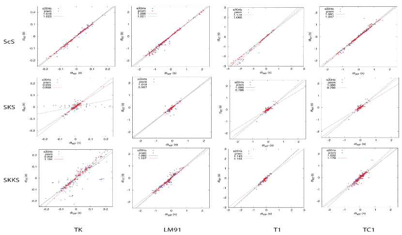
Figure 6: Similar as figure 5. Each row corresponds to a seismic phase (ScS, SKS and SKKS). Most of the phases show better correspondence between predicted and measured by cross-correlation time shift, implying that S-wave phases have a better sensitivity to CMB topography and this can be accommodated by RT.

References

- Helffrich and Wood [2001] G.R. Helffrich and B.J. Wood. The earth’s mantle. Nature, 412:501, 2001.
- Stevenson [1981] D.J. Stevenson. Models of the earth’s core. Science, 214:611–619, 1981.
- Jeanloz and Williams [1998] R. Jeanloz and Q. Williams. The core-mantle boundary region. Ultrahigh-Pressure Mineralogy: Physics and Chemistry of the Earth’s Deep Interior, Rev. Mineral, 37:241–259, 1998. doi:10.1111/j.1365-246X.2011.04970.x.
- Gurnis et al. [1998] M. Gurnis, M.E. Wysession, E. Knittle, and B.A. Buffett. The core-mantle boundary region. AGU, Washington, 1998.
- Lay et al. [1998] T. Lay, Q. Williams, and E. Garnero. The core–mantle boundary layer and deep earth dynamics. Science, 392:461–468, 1998. doi:doi.org/10.1038/33083.
- Bloxham and Jackson [1992] J. Bloxham and A. Jackson. Time-dependent mapping of the magnetic field at the core-mantle boundary. J. Geophys. Res., 97(B13):19537–19563, 1992. doi:doi:10.1029/92JB01591.
- Amit et al. [2015] H. Amit, F. Deschamps, and G. Choblet. Numerical dynamos with outer boundary heat flux inferred from probabilistic tomography - consequences for latitudinal distribution of magnetic flux. Geophys. J. Int., 203:840–855, 2015. doi:10.1093/gji/ggv332.
- Gubbins and Richards [1986] David Gubbins and Mark Richards. Coupling of the core dynamo and mantle: Thermal or topographic? Geophys. Res. Lett., 13:1521–1524, 1986. doi:doi.org/10.1029/GL013i013p01521.
- Calkins et al. [2012] Michael A. Calkins, Jérôme Noir, Jeff D. Eldredge, and Jonathan M. Aurnou. The effects of boundary topography on convection in Earth’s core. Geophys. J. Int., 189(2):799–814, 2012. ISSN 0956540X. doi:10.1111/j.1365-246X.2012.05415.x.
- Davies et al. [2014] Christopher J. Davies, Dave R. Stegman, and M. Dumberry. The strength of gravitational core-mantle coupling. Geophys. Res. Lett., 41:3786–3792, 2014. doi:doi.org/10.1002/2014GL059836.
- Creager and Jordan [1986] Kenneth C. Creager and Thomas H. Jordan. Aspherical structure of the core-mantle boundary from PKP travel times. Geophys. Res. Lett., 13(13):1497–1500, 1986. ISSN 19448007. doi:10.1029/GL013i013p01497.
- Doornbos and Hilton [1989] D J Doornbos and T. Hilton. Models of core-mantle boundary and the travel times of internally reflected core phases. J. Geophys. Res., 94:15741–15751, 1989.
- Shen et al. [2016] Zhichao Shen, Sidao Ni, Wenbo Wu, and Daoyuan Sun. Short period ScP phase amplitude calculations for core-mantle boundary with intermediate scale topography. Physics of the Earth and Planetary Interiors, 253:64–73, 2016. ISSN 00319201. doi:10.1016/j.pepi.2016.02.002. URL http://dx.doi.org/10.1016/j.pepi.2016.02.002.
- Schlaphorst et al. [2016] David Schlaphorst, Christine Thomas, Richard Holme, and Rafael Abreu. Investigation of core-mantle boundary topography and lowermost mantle with P4KP waves. Geophysical Journal International, 204(2):1060–1071, 2016. ISSN 1365246X. doi:10.1093/gji/ggv496.
- Wu et al. [2014] Wenbo Wu, Sidao Ni, and Zhichao Shen. Constraining the short scale core-mantle boundary topography beneath Kenai Peninsula (Alaska) with amplitudes of core-reflected PcP wave. Phys. Earth Planet. In., 236:60–68, 2014. ISSN 00319201. doi:10.1016/j.pepi.2014.09.001. URL http://dx.doi.org/10.1016/j.pepi.2014.09.001.
- Restivo and Helffrich [2006] Andrea Restivo and George Helffrich. Core-mantle boundary structure investigated using SKS and SKKS polarizartion anomalies. Geophysical Journal International, 165(1):288–302, 2006. ISSN 0956540X. doi:10.1111/j.1365-246X.2006.02901.x.
- Sze and van der Hilst [2003] Edmond K.M. Sze and Robert D. van der Hilst. Core mantle boundary topography from short period PcP, PKP, and PKKP data. Physics of the Earth and Planetary Interiors, 135(1):27–46, 2003. ISSN 00319201. doi:10.1016/S0031-9201(02)00204-2.
- Morelli and Dziewonski [1987] A Morelli and Adam M. Dziewonski. Topography of the core-mantle boundary and lateral heterogeneity of the inner core. Nature, 325:678–683, 1987.
- Obayashi and Fukao [1997] M. Obayashi and Y. Fukao. P and pcp travel time tomography for the core-mantle boundary. Geophys. J. R. Astron. Soc., 102:17825–17841, 1997.
- Rodgers and Wahr [1993] A. Rodgers and J. Wahr. Inference of core-mantle boundary topography from isc pcp and pkp traveltimes. Geophys. J. Int., 115:991–1011, 1993.
- Mancinelli and Shearer [2016] Nicholas Mancinelli and Peter Shearer. Scattered energy from a rough core-mantle boundary modeled by a Monte Carlo seismic particle method: Application to PKKP precursors. Geophys. Res. Lett., 43(15):7963–7972, 2016. ISSN 19448007. doi:10.1002/2016GL070286.
- Tanaka [2010] Satoru Tanaka. Constraints on the core-mantle boundary topography from P4 KP-PcP differential travel times. Journal of Geophysical Research, 115(B4):1–14, 2010. ISSN 0148-0227. doi:10.1029/2009jb006563.
- Ishii and Tromp [1999] M. Ishii and J. Tromp. Normal-mode and free-air gravity constraints on lateral variations in velocity and density of earth’s mantle. Science, 285:1231–1236, 1999.
- Xiang-Dong Li et al. [1991] Xiang-Dong Li, D. Giardini, and J. H. Woodhouse. Large-scale three-dimensional even-degree structure of the Earth from splitting of long-period normal modes. Journal of Geophysical Research, 96(B1):551–577, 1991. ISSN 01480227.
- Soldati et al. [2013] Gaia Soldati, Paula Koelemeijer, Lapo Boschi, and Arwen Deuss. Constraints on core-mantle boundary topography from normal mode splitting. Geochemistry, Geophysics, Geosystems, 14(5):1333–1342, 2013. ISSN 15252027. doi:10.1002/ggge.20115.
- Becker and Boschi [2002] Thorsten W. Becker and Lapo Boschi. A comparison of tomographic and geodynamic mantle models. Geochemistry, Geophysics, Geosystems, 3(1), 2002. doi:https://doi.org/10.1029/2001GC000168.
- Koelemeijer [2020] Paula Koelemeijer. Towards consistent seismological models of the core-mantle boundary landscape. Earth and Space Science Open Archive, page 52, 2020. doi:10.1002/essoar.10502426.1. URL https://doi.org/10.1002/essoar.10502426.1.
- Hirose et al. [2017] Kei Hirose, Ryosuke Sinmyo, and John Hernlund. Perovskite in Earth’s deep interior. Science, 358(6364):734–738, 2017. ISSN 10959203. doi:10.1126/science.aam8561.
- Cobden et al. [2015] L. Cobden, C. Thomas, and J. Trampert. Seismic detection of post-perovskite inside the earth. The Heterogeneous Mantle, pages 391–440, 2015. doi:10.1007/978-3-319-15627-9_13.
- Yu and Garnero [2018] S. Yu and E.J. Garnero. Ultralow velocity zone locations: a global assessment. G3, 19:396–414, 2018. doi:10.1002/2017GC007281.
- Hung et al. [2005] Shu-huei Hung, Edward J. Garnero, Ling-yun Chiao, Ban-Yuan Kuo, and Thorne Lay. Finite frequency tomography of D" shear velocity heterogeneity beneath the Caribbean. Journal of Geophysical Research: Solid Earth, 110(B7):1–20, 2005. doi:10.1029/2004JB003373.
- Whittaker et al. [2015] Stefanie Whittaker, Michael S Thorne, Nicholas C Schmerr, and Lowell Miyagi. Seismic array constraints on the D" discontinuity beneath Central America. Journal of Geophysical Research: Solid Earth, 121(1):152–169, 2015.
- Borgeaud et al. [2017] Anselme F. E. Borgeaud, Kenji Kawai, Kensuke Konishi, and Robert J. Geller. Imaging paleoslabs in the Dl̈ayer beneath Central America and the Caribbean using seismic waveform inversion. Science Advances, 3(11), nov 2017. ISSN 2375-2548. doi:10.1126/sciadv.1602700.
- Li and Romanowicz [1996] Xiang-Dong Li and Barbara Romanowicz. Global mantle shear velocity model developed using nonlinear asymptotic coupling theory. Journal of Geophysical Research: Solid Earth, 101(B10):22245–22272, 1996. doi:https://doi.org/10.1029/96JB01306. URL https://agupubs.onlinelibrary.wiley.com/doi/abs/10.1029/96JB01306.
- Ritsema et al. [2011] J. Ritsema, A. Deuss, H.J. van Heijst, and J.H. Woodhouse. S40rts:a degree-40 shear-velocity model for the mantle from new rayleigh wave dispersion, teleseismic traveltime and normal-mode splitting function measurements. Geophys. J. Int., 184(3):1223–1236, 2011.
- Lekic et al. [2012] Vedran Lekic, Sanne Cottaar, Adam Dziewonski, and Barbara Romanowicz. Cluster analysis of global lower mantle tomography: A new class of structure and implications for chemical heterogeneity. Earth and Planetary Science Letters, 357-358:68–77, 2012. ISSN 0012-821X. doi:https://doi.org/10.1016/j.epsl.2012.09.014. URL https://www.sciencedirect.com/science/article/pii/S0012821X12005109.
- Garnero et al. [2016] E.J. Garnero, A.K. McNamara, and S.-H.Z Shim. Continent-sized anomalous zones with low seismic velocity at the base of earth’s mantle. Nat. Geosci., 9(7):481–489, 2016.
- McNamara [2018] A.K. McNamara. A review of large low shear velocity provinces and ultra low velocity zones. Tectonophysics, 760:199–220, 2018.
- Lassak et al. [2010] T.M. Lassak, A.K. McNamara, E.J. Garnero, and S. Zhong. Core–mantle boundary topography as a possible constraint on lower mantle chemistry and dynamics. epsl, 289:232–241, 2010. doi:10.1016/j.epsl.2009.11.012.
- Deschamps et al. [2018] Frédéric Deschamps, Yves Rogister, and Paul J. Tackley. Constraints on core-mantle boundary topography from models of thermal and thermochemical convection. Geophys. J. Int., 212(1):164–188, 2018. ISSN 1365246X. doi:10.1093/gji/ggx402.
- Garcia and Souriau [2000] R. Garcia and A. Souriau. Amplitude of the core–mantle boundary topography estimated by stochastic analysis of core phases. Phys. Earth Planet. In., 117:345–359, 2000.
- Garnero [2000] Edward J. Garnero. Heterogeneity of the lowermost mantle. Annual Review of Earth and Planetary Sciences, 28(1):509–537, 2000. doi:10.1146/annurev.earth.28.1.509. URL https://doi.org/10.1146/annurev.earth.28.1.509.
- Tanaka [2002] Satoru Tanaka. Very low shear wave velocity at the base of the mantle under the South Pacific Superswell. Earth and Planetary Science Letters, 203(3-4):879–893, 2002. ISSN 0012821X. doi:10.1016/S0012-821X(02)00918-4.
- Muir and Tkalčić [2020] J.B. Muir and H. Tkalčić. Probabilistic lowermost mantle P-wave tomography from hierarchical Hamiltonian Monte Carlo and model parametrization cross-validation. Geophysical Journal International, 223(3):1630–1643, 09 2020. ISSN 0956-540X. doi:10.1093/gji/ggaa397. URL https://doi.org/10.1093/gji/ggaa397.
- Colombi et al. [2012] Andrea Colombi, Tarje Nissen-Meyer, Lapo Boschi, and Domenico Giardini. Seismic waveform sensitivity to global boundary topography. Geophys. J. Int., 191(2):832–848, 2012. ISSN 0956540X. doi:10.1111/j.1365-246X.2012.05660.x.
- Colombi et al. [2014] Andrea Colombi, Tarje Nissen-meyer, Lapo Boschi, and Domenico Giardini. Seismic waveform inversion for core–mantle boundary topography. Geophys. J. Int., 198:55–71, 2014. doi:10.1093/gji/ggu112.
- Nissen-Meyer et al. [2014] T. Nissen-Meyer, M. van Driel, S. C. Stähler, K. Hosseini, S. Hempel, L. Auer, A. Colombi, and A. Fournier. Axisem: broadband 3-d seismic wavefields in axisymmetric media. Solid Earth, 5(1):425–445, 2014. doi:10.5194/se-5-425-2014. URL https://se.copernicus.org/articles/5/425/2014/.
- Marquering et al. [1999] Henk Marquering, F.A. Dahlen, and Guust Nolet. Three-dimensional sensitivity kernels for finite-frequency traveltimes: the banana-doughnut paradox. Geophysical Journal International, 137(3):805–815, 06 1999. ISSN 0956-540X. doi:10.1046/j.1365-246x.1999.00837.x. URL https://doi.org/10.1046/j.1365-246x.1999.00837.x.
- Dahlen [2005] F.A. Dahlen. Finite-frequency sensitivity kernels for boundary topography perturbations. Geophys. J. Int., 162:525–540, 2005.
- Tromp et al. [2005] Jeroen Tromp, Carl Tape, and Qinya Liu. Seismic tomography, adjoint methods, time reversal and banana-doughnut kernels. Geophys. J. Int., 160(1):195–216, 2005. doi:10.1111/j.1365-246X.2004.02453.x.
- Komatitsch and Tromp [1999] D. Komatitsch and J. Tromp. Introduction to the spectral element method for three-dimensional seismic wave propagation. Geophys. J. Int., 139(3):806–822, 1999. doi:10.1046/j.1365-246x.1999.00967.x.
- Komatitsch and Tromp [2002a] D. Komatitsch and J. Tromp. Spectral-element simulations of global seismic wave propagation-I. Validation. Geophys. J. Int., 149(2):390–412, 2002a. doi:10.1046/j.1365-246X.2002.01653.x.
- Komatitsch and Tromp [2002b] D. Komatitsch and J. Tromp. Spectral-element simulations of global seismic wave propagation-II. 3-D models, oceans, rotation, and self-gravitation. Geophys. J. Int., 150(1):303–318, 2002b. doi:10.1046/j.1365-246X.2002.01716.x.
- Bai et al. [2012] L. Bai, Y. Zhang, and J. Ritsema. An analysis of SS precursors using spectral-element method seismograms. Geophys. J. Int., 188:293–300, 2012. doi:10.1111/j.1365-246X.2011.05256.x.
- Koroni and Trampert [2016] M. Koroni and J. Trampert. The effect of topography of upper mantle discontinuities on SS precursors. Geophys. J. Int., 204:667–681, 2016.
- Crotwell et al. [1999] H. P. Crotwell, T. J. Owens, and J. Ritsema. The TauP ToolKit: Flexible Seismic Travel-Time and Raypath Utilities. Seismological Research Letters, 70:154–160, 1999.
- Dziewoński and Anderson [1981] A. M. Dziewoński and D. L. Anderson. Preliminary reference Earth model. Phys. Earth Planet. In., 25:297–356, 1981.
- Ritsema and van Heijst [2002] J. Ritsema and H. J. van Heijst. Constraints on the correlation of p- and s-wave velocity heterogeneity in the mantle from p, pp, ppp, and pkpab traveltimes. Geophys. J. Int., 149:482–489, 2002.
- Rawlinson and Kennett [2004] N. Rawlinson and B. L.N. Kennett. Rapid estimation of relative and absolute delay times across a network by adaptive stacking. Geophysical Journal International, 157(1):332–340, 2004. ISSN 0956540X. doi:10.1111/j.1365-246X.2004.02188.x.
- Dahlen et al. [2000] F.-A. Dahlen, S.-H Hung, and Guust Nolet. Fréchet kernels for finite frequency traveltimes-I. theory. Geophys. J. Int., 141:157–174, 2000.
- Liu and Tromp [2008] Qinya Liu and Jeroen Tromp. Finite-frequency sensitivity kernels for global seismic wave propagation based upon adjoint methods. Geophysical Journal International, 174(1):265–286, jul 2008. ISSN 0956540X. doi:10.1111/j.1365-246X.2008.03798.x.
- Luo and Schuster [1991] Y. Luo and G. Schuster. Wave-equation traveltime inversion. GeoRef, 1991. doi:10.1190/1.1443081.
- French and Romanowicz [2014] S. W. French and Barbara A. Romanowicz. Whole-mantle radially anisotropic shear velocity structure from spectral-element waveform tomography. Geophys. J. Int., 199(3):1303–1327, 2014. doi:10.1093/gji/ggu334.
- Favier and Chevrot [2003] N. Favier and S. Chevrot. Sensitivity kernels for shear wave splitting in transverseisotropic media. Geophys. J. Int., 153:213–228, 2003.
- Sieminski et al. [2008] A. Sieminski, H. Paulssen, J. Trampert, and J. Tromp. Finite-frequencyskssplitting: Measurement and sensitivity kernels. BSSA, 98:1797–1810, 2008. doi:doi: 10.1785/0120070297.
- Souriau and Poupinet [1991] Annie Souriau and Georges Poupinet. A study of the outermost liquid core using differential travel times of the sks, skks and s3ks phases. Physics of the Earth and Planetary Interiors, 68(1):183–199, 1991. ISSN 0031-9201. doi:https://doi.org/10.1016/0031-9201(91)90017-C. URL https://www.sciencedirect.com/science/article/pii/003192019190017C.
- Aki and Richards [1980] K. Aki and P. G. Richards. Quantitative seismology, theory and methods. W. H. Freeman, San Francisco, USA, 1980.
- Doornbos and Mondt [1980] D. J. Doornbos and J. C. Mondt. Sthe interaction of elastic waves with a solid-liquid interface, with applications to the core-mantle boundary. Pure and Applied Geophysics, 118:1293–1309, 1980.
- Earle and Shearer [1997] Paul S. Earle and Peter M. Shearer. Observations of pkkp precursors used to estimate small-scale topography on the core-mantle boundary. Science, 277:667–670, 1997. doi:DOI: 10.1126/science.277.5326.667.
- Rost and Revenaugh [2003] Sebastian Rost and Justin Revenaugh. Detection of a d" discontinuity in the south atlantic using pkkp. Geophysical Research Letters, 30(16), 2003. doi:https://doi.org/10.1029/2003GL017585. URL https://agupubs.onlinelibrary.wiley.com/doi/abs/10.1029/2003GL017585.
- Koroni et al. [2019] Maria Koroni, Hanneke Paulssen, and Jeannot Trampert. Sensitivity kernels of pp precursor traveltimes and their limitations for imaging topography of discontinuities. Geophys. Res. Lett., 46(2):698–707, 2019. doi:10.1029/2018GL081592.