RefRec: Pseudo-labels Refinement via Shape Reconstruction
for Unsupervised 3D Domain Adaptation

Abstract

Unsupervised Domain Adaptation (UDA) for point cloud classification is an emerging research problem with relevant practical motivations. Reliance on multi-task learning to align features across domains has been the standard way to tackle it. In this paper, we take a different path and propose RefRec, the first approach to investigate pseudo-labels and self-training in UDA for point clouds. We present two main innovations to make self-training effective on 3D data: i) refinement of noisy pseudo-labels by matching shape descriptors that are learned by the unsupervised task of shape reconstruction on both domains; ii) a novel self-training protocol that learns domain-specific decision boundaries and reduces the negative impact of mislabelled target samples and in-domain intra-class variability. RefRec sets the new state of the art in both standard benchmarks used to test UDA for point cloud classification, showcasing the effectiveness of self-training for this important problem.

1 Introduction

Properly reasoning on 3D geometric data such as point clouds or meshes is crucial for many 3D computer vision tasks, which are key to enable emerging applications like autonomous driving, robotic perception and augmented reality. In particular, assigning the right semantic category to a set of points that represent the surface of an object is a required skill for an intelligent system in order to understand the 3D scene around it. Such problem, referred to as shape classification, was initially addressed by hand-crafted features [20, 4, 44], while, with the advances in deep learning, recent proposals learn features directly from 3D point coordinates by means of deep neural networks [37, 38, 28, 63, 62, 27, 18, 58, 49, 24]. Although data-driven approaches can achieve impressive results, they require massive amounts of labeled data to be trained, which are cumbersome and time-consuming to collect. Typically, 3D deep learning methods use synthetic datasets of CAD models, e.g. ModelNet40 [60] or ShapeNet [6], to harvest a large number of 3D examples. While synthetic datasets enable 3D deep learning, they create a conundrum. On the one hand, shape classifiers trained on ModelNet are very effective on synthetic data, as witnessed by performance saturation on standard benchmarks [54, 14]. On the other hand, though, they are not able to transfer their performance to real-world scenarios [54], where point cloud data are usually captured by RGB-D or LiDAR sensors [10, 17]. This limitation severely restricts the deployment of 3D deep learning methods in real-world applications.

Figure 1: Feature space of a classifier (left) and a reconstruction auto-encoder (right). A classifier trained on source shapes only (blue) may not be effective on target shapes (orange) and assign wrong pseudo-labels. An auto-encoder, instead, tends to cluster similar shapes together in the learned embedding, such that its features can be used as global shape descriptors to correct wrong pseudo-labels.

Unsupervised Domain adaptation (UDA) aims at bridging this domain shift [50] by learning to transfer the knowledge gained on a labeled dataset, i.e. source domain, to an unlabeled target dataset, i.e. target domain.

UDA has its roots in 2D computer vision, where a multitude of methods have been proposed [22]. Among them, the most widespread approach pertains globally aligning the feature distributions between the source and target domain. This is the paradigm also leveraged by methods tackling UDA for 3D data, either explicitly, by designing losses and models to align features [39], or implicitly, by solving a self-supervised task on both the source and target domains with a shared encoder [3, 1]. We argue that, when moving from a synthetic CAD dataset to a real world one, feature alignment can only lead to sub-optimal solutions due to the large differences between the two domains. Indeed, acquiring objects in cluttered scenes results oftentimes in partial scans with missing parts due to occlusions. Moreover, registration errors arising when fusing multiple 2.5D scans [11] to obtain a full 3D shape, alongside noise from the sensor, result in less clean and geometrically coherent shapes than CAD models (see Fig. 3). Therefore, the shape classifier may need to ground its decision on new cues, different from those learned on the source domain, where the clean full shape is available, to correctly classify target samples.

To let the classifier learn such new cues, in this paper we propose RefRec (Refinement via Reconstruction), a novel framework to perform unsupervised domain adaptation for point cloud classification. Key to our approach is reliance on pseudo-labels [23], i.e. predictions on the target domain obtained by running a model trained on the source domain, which are then used as a noisy supervision to train a classifier on the target domain and let it learn the domain-specific cues. This process is usually referred to as self-training [23, 66]. However, the pseudo-labels obtained from a model trained on the source domain may be wrong due to the domain shift (as shown in Fig. 1-left) and a target domain classifier naively trained on them would underperform. Therefore, our key contribution concern effective approaches to refine pseudo-labels. We propose both an offline and an online refinement, i.e. before training and while training on pseudo-labels. Both refinements are based on the idea that similar shapes should share similar labels. To find similar shapes, we match global shape descriptors, i.e. the embedding computed by an encoder given the input shape. Here we make another key observation, illustrated in Fig. 1: the space of features learned by a classifier is organized to create linear boundaries among different classes, but it is not guaranteed -nor meant- to posses a structure where similar shapes lay close one to another, especially for target samples which are not seen at training time. Hence, such features are not particularly effective if used as global shape descriptors. In contrast, teaching a point cloud auto-encoder to reconstruct 3D shapes is an effective technique to obtain a compact and distinctive representation of the input geometric structures, as proven by recent proposals for local and global shape description [64, 15, 12, 45], which, in our setting, can be trained also on the target domain since it is learned in an unsupervised way. By leveraging on such properties of the reconstruction latent space, in the offline step we focus on reassigning the pseudo-labels of target samples where the source domain classifier exhibits low confidence, while in the online step we compute prototypes [36], i.e. the mean global descriptors on the target domain for each class, and we weight target pseudo-labels according to the similarity of the input shape to its prototype. Peculiarly, by using reconstruction embeddings trained also on the target domain to compute prototypes, we avoid the domain shift incurred when using the classifier trained on the source domain as done by previous 2D methods [19]. In the online refinement step, we also leverage the standard training protocol of 2D UDA methods based on mean teacher [48] to improve the quality of pseudo-labels as training progresses.

We can summarize our contributions as follows:

1. we investigate on self-training to solve UDA for point clouds, an approach that sharply differs from existing proposals in literature based on multi-task learning. To the best of our knowledge, this work is the first to study this alternative path;

2. we show how global descriptors learned for shape reconstruction can be effectively used both offline and online to refine pseudo-labels in UDA for point cloud classification;

3. we show how effective techniques for 2D UDA, like domain-specific classifiers and mean teacher supervision, can be successfully used on 3D data;

4. we achieve new state of the art performance on the standard benchmarks used to assess progress in UDA for point cloud classification.

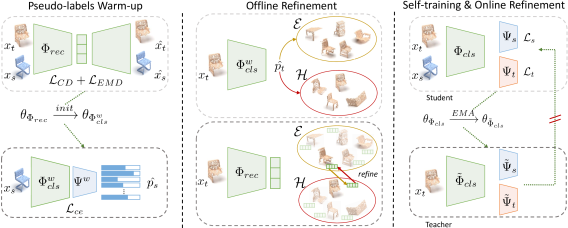
Figure 2: RefRec comprises three steps. First, in the pseudo-labels warm up step, we train a reconstruction network $\Phi_{rec}$ on both source and target domains. The weights of the encoder are used to initialize the backbone $\Phi^{w}_{cls}$ of a classifier, that is then trained on the source domain. In the refinement step, we use the classifier to split target samples in the easy ($\mathcal{E}$) and hard ($\mathcal{H}$) sets according to their confidence and refine them by performing nearest neighbor queries in the auto-encoder feature space. Finally, in the self-training step, we train a target-specific classifier $\Psi_{t}$ by refined pseudo-labels and online pseudo-labels obtained with the mean teacher architecture [48].

2 Related Work

2.1 Unsupervised Domain Adaptation (UDA)

Unsupervised Domain Adaptation aims at reducing the need of large amounts of annotated data. The key idea is to learn distinctive and powerful features in the source domain and exploit such representation in the target domain. A remarkable amount of work has been conducted for image classification [13, 5, 30, 29, 47, 52, 53, 25], semantic segmentation [26, 51, 7, 16, 59, 21] and object detection [9, 56, 56, 57, 42]. The most common approach to tackle UDA is to minimize the discrepancy between domains to obtain domain-invariant features, so that the same classifier can be deployed in both domains. Alignment in feature space can be achieved by forcing features from both domain to have similar statistics, as done in [30, 29]. Another interesting line of research, instead, casts domain alignment as a min-max problem, exploiting adversarial training to attain such alignment. For example, Tzeng et al. [52] introduced a domain confusion loss to obtain features indistinguishable across domains. Ganin et al. [13] try to learn domain invariant representations in an adversarial way by back-propagating the reverse gradients of the domain classifier. All these methods are meant to work with images and do not explore any variations or extensions to exploit 3D data. In this work, instead, we turn our attention on 3D data and focus on their peculiar properties to design an effective domain adaptation methodology.

2.2 Unsupervised 3D Domain Adaptation

Only few papers discuss Unsupervised Domain Adaptation for point cloud classification. Among these, PointDAN [39] is a seminal work that proposes to adapt a classical 2D domain adaptation approach to the 3D world. Specifically, they focus on the alignment of both local and global features, building their framework upon the popular Maximum Classifier Discrepancy (MCD) [43] for global feature alignment. Differently, [3, 1] leverage on Self-supervised learning (SSL) to learn simultaneously distinctive features for both the source and target domains. Similarly, [3] also relays on SSL, and introduces a novel pretext task to learn strong features for the target domain as well. In this work, we take one step further and present an unsupervised domain adaptation method based on pseudo-labels that exploits a shape reconstruction task to refine them.

2.3 Deep Learning for Point Clouds Reconstruction

With the recent advances in deep learning several methods for point cloud reconstruction have been suggested. A seminal work in this area [2] proposes a new auto-encoder architecture for point clouds using the permutation invariant operator introduced in [37]. AtlasNet [15] and FoldingNet [64] propose a plane-folding decoder to learn to deform points sampled from a plane in order to reconstruct the input surface. TearingNet [33] takes inspiration from [64, 15] and present a tearing module to cut regular 2D patch with holes, or into several parts, to preserve the point cloud topology. In [8], the authors reconstruct the point clouds by training a generative adversarial network (GAN) on the latent space of unpaired clean synthetic and occluded real point clouds. We take inspiration from the finding of [2] and leverage the expressive power of point cloud auto-encoders to pre-train our shape classifier and learn a global shape descriptor deployed for pseudo-labels refinement.

3 Method

In this work, we address UDA for point clouds classification. Hence, we assume availability of a labeled source domain $\mathcal{S}={\{(\textbf{x}_{s}^{i}\in\mathcal{X}_{s},y_{s}^{i}\in\mathcal{Y}_{s})\}_{i=1}^{n_{s}}}$, and a target domain $\mathcal{T}=\{\textbf{x}_{t}^{j}\in\mathcal{X}_{t}\}_{j=1}^{n_{t}}$, whose labels $\{y_{t}^{j}\in\mathcal{Y}_{t}\}_{j=1}^{n_{t}}$ are, however, not available. As in standard UDA settings [55], we assume to have the same one-hot encoded label space $\mathcal{Y}_{s}=\mathcal{Y}_{t}=\mathcal{Y}=\{0,1\}^{k}$ and the same input space $\mathcal{X}_{s}=\mathcal{X}_{t}$ (i.e. point clouds with $\{x,y,z\}$ coordinates) but with different distributions $P_{s}(\textbf{x})\neq P_{t}(\textbf{x})$, e.g. due to source data being synthetic while target data being real or due to the use of different sensors. The final classifier for a point cloud x can be obtained as a composite function $\Omega=\Phi\circ\Psi$, with $\Phi:\mathcal{X}\rightarrow\mathbb{R}^{d}$ representing the feature extractor and $\Psi:\mathbb{R}^{d}\rightarrow[0,1]^{k}$ the classification head, which outputs softmax scores $\hat{\mathbf{p}}\in[0,1]^{k}$. When one-hot labels are needed, we further process softmax scores with $\Lambda:\mathbb{R}^{k}\rightarrow\mathcal{Y}$ to obtain the label corresponding to the largest softmax score, with such value

providing also the confidence associated with the label prediction. Although the largest softmax is a rather naive confidence measure, we found it to work satisfactorily in our experiments. Our overall goal is to learn a strong classifier $\Omega_{t}$ for the target domain even though annotations are not available therein.

An overview of our method is depicted in Fig. 2. It encompasses three major steps: warm-up, pseudo-labels refinement, and self-training. The purpose of the first step, described in Sec. 3.1, is to train a model effective on target data by using labelled source data and unlabelled target data. Once trained, this model provides the initial pseudo-labels. These are refined offline in the second step, described in Sec. 3.2, in order to partially reduce the errors in pseudo-labels due to the limited generalization of the source classifier to the target domain. Finally, in the last step, detailed in Sec. 3.3, we introduce an effective way of exploiting pseudo-labels during self-training by combining a domain-specific classifier with an online pseudo-labels weighting strategy that exploits prototypes computed in the target domain.

3.1 Pseudo-labels Warm-up

The first step of our pipeline seeks to produce good initial pseudo-labels, which, after refinement, can be used to train the final classifier on the source domain and the target domain augmented with pseudo-labels. The warm-up step is very important, as the effectiveness of self-training is directly related to the quality of pseudo-labels. To obtain good initial pseudo-labels, we focus on pretraining and data augmentation, with the aim of reducing overfitting on source data. Pre-training is largely adopted also in UDA for image classification, where ImageNet pre-training is a standard procedure [19, 35, 30] that learns powerful features able to generalize to multiple domains and alleviates the risk of overfitting when training solely on data coming from the source distribution. Differently from UDA in the 2D world, however, here we focus on unsupervised pre-training. This is particularly attractive for the UDA context, where no supervision is available for the target domain. In fact, inspired by recent advances on representation learning for 3D point clouds, which have demonstrated the effectiveness of unsupervised techniques for learning discriminative features [64, 15, 12, 45], we propose to use point cloud reconstruction as unsupervised pre-training for our backbone. The key advantage of such pre-training is the possibility to capture discriminative features also for the target domain since unsupervised pre-training can be conducted on both domains simultaneously. Moreover, it learns a feature extractor $\Phi_{rec}$ which can be deployed also to refine labels effectively, as we do in the following steps of our pipeline.

We follow the same strategy proposed in [2], and use a standard PointNet [37] backbone as $\Phi_{rec}$ to produce a global $d$-dimensional descriptor of the input point cloud. This latent representation is then passed to a simple decoder made out of 3 fully connected layers that tries to reconstruct the original shape. During training we minimize both the Chamfer Discrepancy (CD) $\mathcal{L}_{CD}$ and Earth Mover’s distance (EMD) $\mathcal{L}_{EMD}$ [41] as loss functions [2]. Additionally, as mentioned above, data augmentation is a key ingredient to improve generalization, especially for the synthetic-to-real adaptation case, since 3D real scans always exhibits occlusions and non-uniform point density. For this reason, when performing synthetic-to-real adaptation, we apply a data augmentation procedure similar to that proposed in [46] in order to simulate occlusions.

To conclude warm-up, we train a new classifier $\Omega^{w}=\Phi^{w}_{cls}\circ\Psi^{w}$ on the source dataset with a classical cross-entropy loss. Importantly, $\Phi^{w}_{cls}$ and $\Phi_{rec}$ have the same architecture and the weights $\theta$ of the backbone ${\Phi^{w}_{cls}}$ are initialized with those learned for $\Phi_{rec}$. We then use $\Omega^{w}$ to obtain pseudo-labels $\{\hat{y}^{j}_{t}=\Lambda(\Omega^{w}(\mathbf{x}^{j}_{t})\}_{j=1}^{n_{t}})$ alongside their confidence scores.

We may, in principle, exploit these pseudo-labels to perform self-training in the target domain. However, even if we rely on unsupervised pre-training and data augmentation to boost performance on the target domain, they are still noisy. Indeed, due to the domain gap, only a small portion of the pseudo-labels can be considered reliable, while the majority of the samples are assigned wrong labels that could lead to poor performance when applying self-training. Hence, in the next step, we refine the initial pseudo-labels obtained in the warm-up step by leveraging on $\Phi^{w}_{rec}$.

3.2 Pseudo-labels Refinement

To refine pseudo-labels, we exploit the confidence computed by the classifier $\Omega^{w}$ and split pseudo-labels in the two disjoint sets of highly confident predictions, denoted as $\mathcal{E}$ (i.e. easy split), and uncertain ones, denoted as $\mathcal{H}$ (i.e. hard split). We first build $\mathcal{E}$ by selecting the g=10% most confident predictions on the target samples for each class. We perform this operation class-wisely to obtain a sufficient number of examples for each class and to reproduce the class frequencies in $\mathcal{E}$. $\mathcal{H}$ is composed by all the remaining target samples.

One of the key idea behind RefRec is to utilize the embedding of the reconstruction backbone $\Phi_{rec}$, instead of $\Phi^{w}_{cls}$, to improve the labels of the samples in $\mathcal{H}$. We conjecture that since $\Phi^{w}_{cls}$ has been trained only on the source domain, its embeddings are not discriminative for the target domain, and more importantly there are no guarantees that objects belonging to the same class, yet coming from different domains, would lay close in the feature space. Hence, we assign new pseudo-labels to target samples according to similarities in the feature space of $\Phi_{rec}$.

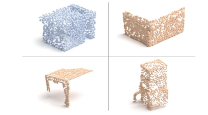
Figure 3: Samples from cabinet. First row: intra-class variability between domains (ModelNet and ScanNet). Second row: intra-class variability in ScanNet.

We first seek to expand the set of easy examples $\mathcal{E}$ by finding in the feature space of $\Phi_{rec}$ the nearest neighbor in $\mathcal{H}$ for each sample of $\mathcal{E}$ and viceversa. To refine pseudo-labels for samples in $\mathcal{H}$, we adopt a well-know technique employed for surface registration [12, 65, 45] and accept only reciprocal nearest neighbor matches, i.e. pairs of samples that are mutually the closest one in the feature space: if one sample $h\in\mathcal{H}$ is the nearest neighbour in $\mathcal{H}$ of a sample $e\in\mathcal{E}$ and $e$ is in turn the nearest neighbor of $h$ in $\mathcal{E}$, we move $h$ to the easy split and label it according to the pseudo-label of $e$. At the end of this procedure we obtain a refined set of easy examples $\mathcal{E}^{r}$.

We then try to refine the pseudo-labels for the samples left in $\mathcal{H}$ exploiting $\mathcal{E}^{r}$. In particular, we select $K$-nearest neighbors ($K=3$ in our experiments) in the refined set $\mathcal{E}^{r}$ for each remaining sample $h\in\mathcal{H}$, and assign the new pseudo-label to $h$ by majority voting. When there is no consensus among the $K$ neighbors, we assign the pseudo-label of the closest one. This produces the refined set of hard examples $\mathcal{H}^{r}$. It is important to note that the entire process is applied offline before the self-training step, as illustrated in Fig. 2, and the absence of hard thresholds in all the refinement steps facilitates the applicability of the proposed method across datasets.

3.3 Self-training

When performing synthetic-to-real adaptation and vice-versa, the gap among the two distributions could be large and difficult to reduce even in case of perfect supervision. As a matter of example, Fig. 3 shows how shapes, such as cabinets, may look very different across domains (first row) as well as within a domain (second row). A high intra-class variability can be somehow dealt with in a supervised setting, but it is harder to handle when noisy supervision in the form of pseudo-labels must be used. Hence, in this setting, it is difficult for a neural network to find common features for shapes belonging to the same class across domains. We address this issue by adopting domain-specific classification heads together with online pseudo-labels refinement while performing the self-training step that concludes our pipeline.

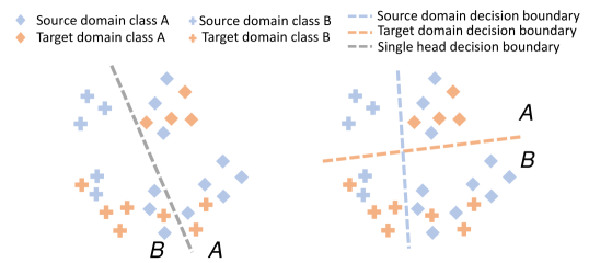
Figure 4: Single head vs domain-specific classification heads. When a single head is deployed (left side), it may not be possible to find a linear decision boundary that correctly classifies both classes for the source and target domain. When domain-specific classification heads are deployed, the model can focus on each domain separately and learn more effective decision boundaries (right side).

Domain-specific classification heads. To tackle intra-class variability across domains, we deploy a shared encoder $\Phi_{cls}$, initialized using the weights from $\Phi_{rec}$, and attach two domain-specific classification heads, $\Psi_{s}$ and $\Psi_{t}$, for the source and target domain, respectively. The benefit of having a target-specific head (right) versus a single head trained on both domains (left) is highlighted in Fig. 4.

When using a single classification head, the model tries to separate classes for both domains simultaneously, which may lead to a non-optimal decision boundary. Indeed, due to the high intra-class variability across the domains it is not possible to find a single decision boundary to correctly separate all samples for both, leading to some wrongly classified samples. When employing two domain-specific heads, instead, the model can learn two more effective boundaries.

Although domain-specific classification heads have been already explored in UDA for image classification [40], in RefRec we can apply them in a unique way, which makes them more effective, as it will been shown in our ablation studies. In particular, we train the first head $\Psi_{s}$ on the source domain mixed with $\mathcal{E}^{r}$, while we supervise the second head using target data only, i.e. both $\mathcal{E}^{r}$ and $\mathcal{H}^{r}$. By doing this, we force both heads to correctly classify the easy split, which contains the most confident predictions, i.e. the set of target samples already more aligned with the source domain. Thereby, training with this strategy does not reduce performance on the source domain while it enforces a partial feature alignment across domains. At the same time, by only feeding target data to $\Psi_{t}$, we let the model define target-specific boundaries, alleviating the negative impact of the intra-class variability across domains.

Online pseudo-labels refinement. Even when using domain-specific classification heads, the intra-class variability on the target domain can still affect the model performance. To deal with this issue we adopt an online pseudo-labels refinement and weighting strategy. The key intuition behind online refinement is that, as training progresses, our classifier better learns how to classify the target domain thanks to the pseudo-labels and thus we can progressively improve the pseudo-labels by exploiting such freshly learned knowledge. Purposely, we exploit the mean teacher [48] of our model in order to obtain online pseudo-labels $\tilde{y}_{t}$:

$$\tilde{y}_{t}=\Lambda(\tilde{\Psi}_{s}(\tilde{\Phi}_{cls}(\mathbf{x}_{t}))+\tilde{\Psi}_{t}(\tilde{\Phi}_{cls}(\mathbf{x}_{t})))$$ (1)

It is important to note that $\tilde{\Phi}_{cls}$, $\tilde{\Psi}_{s}$, and $\tilde{\Psi}_{t}$ are never updated trough gradient back-propagation, as they consists of simple temporal exponential moving averages (EMA )of their student counterparts [48]. At each training step, we feed one batch of samples from $\{\mathcal{S},\mathcal{E}^{r}\}$ and one batch from $\{\mathcal{E}^{r},\mathcal{H}^{r}\}$ to train $\Phi_{cls}\circ\Psi_{s}$ and $\Phi_{cls}\circ\Psi_{t}$, respectively. As for the source classifier, we train it by the standard cross-entropy loss with labels for the source domain and the pseudo-labels $\hat{y}_{t}$ obtained from the refinement step for $\mathcal{E}^{r}$:

$$\mathcal{L}_{s}=\mathcal{L}_{ce}(\mathbf{p}_{s},\mathbf{y}_{s})+\mathcal{L}_{ce}(\mathbf{p}_{t},\hat{\mathbf{y}}_{t})$$ (2)

We instead exploit both the refined ($\hat{\mathbf{y}}_{t}$) and the on-line ($\tilde{\mathbf{y}}_{t}$) pseudo-labels when training the target classifier:

$$\mathcal{L}_{t}=(1-\alpha_{it})z_{t}\mathcal{L}_{ce}(\mathbf{p}_{t},\hat{\mathbf{y}}_{t})+\alpha_{it}z_{t}\mathcal{L}_{ce}(\mathbf{p}_{t},\tilde{\mathbf{y}}_{t})$$ (3)

where $\alpha_{it}$ is a weighting factor that starts from 0 (use only refined pseudo-labels) and increases at every iteration up to 1 (use only on-line pseudo-labels). Intuitively, when self-training starts, we trust the previously refined pseudo-labels and thus give more weight to the first term of Eq. 3 as the mean teacher is not reliable yet. As training goes on, we progressively trust more the output of the mean teacher, i.e. $\tilde{y}_{t}$, and so give more weight to the second term. $z_{t}$ is instead a weighting factor that accounts for the plausibility of the pseudo-label. $z_{t}$ is computed for each target sample exploiting once again the embedding of $\Phi_{rec}$. In particular, before the self-training step, we compute the class-wise prototypes $\eta^{(k)}\in\mathbb{R}^{d}$ as the class-wise average of the target features in the easy split:

$$\eta^{(k)}=\frac{\sum_{x_{t}\in\mathcal{E}^{r}}\Phi_{rec}(x_{t})*\mathbbm{1}(\hat{y}_{t,k}==1)}{\sum_{x_{t}\in\mathcal{E}^{r}}\mathbbm{1}(\hat{y}_{t,k}==1)}$$ (4)

where $\hat{y}_{t,k}$ is the $k$-entry in $\hat{y}_{t}$. We only consider $\mathcal{E}^{r}$ as it contains the most reliable pseudo-labels for the target domain. We then obtain the confidence score for each sample by simply computing the softmax of the opposite of the distance between the current embedding of $x_{t}$ and the prototype of the class $k$ assigned to it in its online pseudo-label, $k=\arg\max_{k^{\prime}}\tilde{y}_{t,k^{\prime}}$:

$$z_{t}=\frac{\exp(-\|\tilde{\Phi}_{cls}(\mathbf{x}_{t})-\eta^{(k)}\|_{2})}{\sum_{k^{\prime}}\exp(-\|\tilde{\Phi}_{cls}(\mathbf{x}_{t})-\eta^{(k^{\prime})}\|_{2})}.$$ (5)

Hence, $z_{t}$ forces the loss to ignore samples which are far from the expected prototype. In fact, when a sample has a very different representation from the expected class prototype, either the pseduo-label is wrong or the input point cloud is an outlier in the target distribution, and dynamically weighting it less in the self-training process allows for learning a better classifier.

Method	ModelNet to	ModelNet to	ShapeNet to	ShapeNet to	ScanNet to	ScanNet to	Avg
	ShapeNet	ScanNet	ModelNet	ScanNet	ModelNet	ShapeNet
No Adaptation	80.2	43.1	75.8	40.7	63.2	67.2	61.7
PointDAN [39]	80.2	45.3	71.2	46.9	59.8	66.2	61.6
DefRec [1]	80.0	46.0	68.5	41.7	63.0	68.2	61.2
DefRec+PCM [1]	81.1	50.3	54.3	52.8	54.0	69.0	60.3
3D Puzzle [3]	81.6	49.7	73.6	41.9	65.9	68.1	63.5
RefRec (Ours)	81.4	56.5	85.4	53.3	73.0	73.1	70.5
Oracle	93.2	64.2	95	64.2	95.0	93.2

Table 1: Shape classification accuracy (%) on the PointDA-10 dataset. For each method, we report the average results on three runs. Best result on each column is in bold.

Method	ModelNet to
	ScanObjectNN
No Adaptation	49.6
PointDAN [39]	56.4
3D Puzzle [3]	58.5
RefRec (Ours)	61.3

Table 2: Shape classification accuracy (%) on the ScanObjectNN dataset. For each method, we report the average results on three runs. Best result is in bold.

4 Experiments

We evaluate our method on two standard datasets for point cloud classification: PointDA-10 [39] and ScanObjectNN [54].

PointDA-10. PointDA-10 is composed by subsets of three widely adopted datasets for point cloud classification: ShapeNet [6], ModelNet40 [61] and ScanNet [10]. The subsets share the same ten classes and can be used to define six different pairs of source/target domains, which belongs to three different adaptation scenarios: real-to-synthetic, synthetic-to-synthetic and synthetic-to-real, with the last one arguably the most relevant to practical applications. ModelNet-10 contains 4183 train samples and 856 tests samples of 3D synthetic CAD models. ShapeNet-10 is a synthetic dataset alike, but exhibits more intra-class variability compared to ModelNet-10. It consists of 17,378 train samples and 2492 test samples. ScanNet-10 is the only real datasets and contains 6110 train and 1769 test samples. ScanNet-10 has been obtained from RGB-D scans of real-world indoor scenes. Due to severe occlusions and noise in the registration process, ScanNet-10 is hard to address even by standard supervised learning, which renders the associated synthetic-to-real UDA setting very challenging. Following previous 3D DA work [39, 3, 1], we uniformly sample 1024 points from each 3D shape for training and testing.

ScanObjectNN. ScanObjectNN is a real-world dataset composed by 2902 3D scans from 15 categories. Similarly to ScanNet-10, it represents a challenging scenario due to the high diversity with respect to synthetic datasets and the presence of artifacts such as non-uniform point density, missing parts and occlusions. Several variants of the ScanObjectNN dataset are provided. As in [3], we select the OBJ_ONLY version which contains only foreground vertices, and test in the synthetic-to-real setting ModelNet40 to ScanObjectNN using the 11 overlapping classes.

4.1 Implementation details

As done in all previous 3D DA methods [39, 3, 1], we use the well-known PointNet [37] architecture. In particular, we use the standard PointNet proposed for point cloud classification for all our backbones $\Phi^{w}_{cls}$, $\Phi_{cls}$, and $\Phi_{rec}$. It produces a 1024 dimensional global feature representation for each input point cloud. We train the reconstruction network for 1000 epochs in the unsupervised pre-training step [2], while we train only for 25 epochs when training classification networks in each step of our pipeline. We set to 0.0001 both learning rate and weight decay. We train with batch size 16 using AdamW [32] with cosine annealing [31] as optimizer. The framework is implemented in PyTorch [34], and is available at https://github.com/CVLAB-Unibo/RefRec. At test time, we use the target classifier $\Phi_{cls}\circ\Psi_{t}\circ\Lambda$ in the target domain.

Experiment		ModelNet to	ModelNet to	ShapeNet to	ShapeNet to	ScanNet to	ScanNet to	Avg
Training data	Offline ref.	ShapeNet	ScanNet	ModelNet	ScanNet	ModelNet	ShapeNet
$\mathcal{S},\mathcal{E},\mathcal{H}$		82.2	51.7	80.4	43.4	64.7	70.0	65.4
$\mathcal{S},\mathcal{E}$		82.8	49.6	79.0	43.8	64.1	69.8	64.9
$\mathcal{S},\mathcal{E}^{r},\mathcal{H}^{r}$	✓	79.1	57.3	85.6	50.7	70.1	69.1	68.7

Table 3: Ablation study on the effect of offline refinement. We report the average shape classification accuracy (%) on three runs.

Experiment				ModelNet to	ModelNet to	ShapeNet to	ShapeNet to	ScanNet to	ScanNet to	Avg
$\Psi_{s}$	$\Psi_{t}$	EMA	Online ref.	ShapeNet	ScanNet	ModelNet	ScanNet	ModelNet	ShapeNet
$\mathcal{S}$	$\mathcal{E}^{r},\mathcal{H}^{r}$			79.5	55.3	84.7	49.3	72.0	68.5	68.2
$\mathcal{S},\mathcal{E}^{r}$	$\mathcal{E}^{r},\mathcal{H}^{r}$			79.3	56.9	84.7	51.6	71.7	69.0	68.9
$\mathcal{S},\mathcal{E}^{r}$	$\mathcal{E}^{r},\mathcal{H}^{r}$	✓		80.3	54.2	83.2	52.7	72.8	71.6	69.1
$\mathcal{S},\mathcal{E}^{r}$	$\mathcal{E}^{r},\mathcal{H}^{r}$	✓	✓	81.4	56.5	85.4	53.3	73.0	73.1	70.5

Table 4: Ablation study on the effect of the self-training strategy and online refinement. We report the average shape classification accuracy (%) on three runs.

Method	ModelNet to	ModelNet to	ShapeNet to	ShapeNet to	ScanNet to	ScanNet to	Avg
	ShapeNet	ScanNet	ModelNet	ScanNet	ModelNet	ShapeNet
No Adaptation	80.2	43.1	75.8	40.7	63.2	67.2	61.7
Warm-up	81.3	51.4	78.9	43.8	59.7	67.5	63.7
Multi-task	80.6	45.4	78.9	46.0	63.9	67.4	63.7
Self-train multi-task	81.2	46.9	76.3	47.7	66.0	66.5	64.1
RefRec (Ours)	81.4	56.5	85.4	53.3	73.0	73.1	70.5

Table 5: Ablation study on the effect of pre-training. We report the average shape classification accuracy (%) on three runs.

4.2 Results

We report and discuss here the results of RefRec, and compare its performance against previous work as well as the baseline method trained on the source domain and tested on the target domain (referred to as No Adaptation). For each experiment, we provide the mean accuracy obtained on three different seeds. Since in UDA target annotations are not available, we never use target labels to perform model selection and we always select the model that gives the best result on the validation set of the source dataset.

PointDA-10. We summarize results for each benchmark in Tab. 1. Overall, our proposal improves by a large margin the previous state-of-the-art methods. Indeed, on average we obtain 70.5% against the 63.5% obtained by 3D puzzle [3], which is an improvement of 7% in terms of accuracy. From Tab. 1, it is also possible to observe how our method is consistently better than previous works in the synthetic-to-real adaptation scenario, which we consider the most important for practical applications. Compared to DefRec+PCM [1], which obtains 50.3 in the ModelNet$\rightarrow$ScanNet setting, we improve by 6.2%. As regards ShapeNet$\rightarrow$ScanNet, we obtain 53.3, surpassing by 0.5% DefRec+PCM again. Moreover, we highlight how RefRec seems to be the only framework able to generalize well to all adaptation scenarios. In fact, when comparing our proposal to DefRec+PCM which was the strongest method for the synthetic-to-real case, we also improve by a large margin in cases such as ShapeNet$\rightarrow$ModelNet and ScanNet$\rightarrow$ModelNet, where DefRec+PCM seems to fail. Finally, the ability of RefRec to handle large distributions gaps is also confirmed by the large improvements in the real-to-synthetic cases. Indeed, we observe a +7.1% improvement for ScanNet$\rightarrow$ModelNet and +4.1% for ScanNet$\rightarrow$ShapeNet.

ScanObjectNN. In Tab. 2 We report the results for the challenging ModelNet$\xrightarrow{}$ScanObjectNN adapation task. On this challenging benchmark, we achieve 61.3%, which is 2.8% better that the previous state-of-the-art result.

4.3 Ablation studies

To validate the importance of our design choices, we conduct some ablation studies on both the pseudo-labels refinement process and the self-training strategy.

Pseudo labels refinement. In Tab. 3, we show the effect of our refinement process. When performing self-training with the initial, unrefined pseudo-labels produced by the classifier $\Psi_{s}$ after the warm-up step (first row), we obtain an overall accuracy of 65.4%. Conversely, when we apply our descriptor matching approach aimed at pseudo-labels refinement (third row), the accuracy increases to 68.7%. This confirms our intuition that using the reconstruction network allows to capture similarities among shapes in feature space and consequently to improve the pseudo-labels. Moreover, we compare self-training using the most-confident pseudo-labels only (second row) against self-training with the refined pseudo-labels (third row). The improvement given by the refinement approach (+3.8%) suggests that only using the most confident pseudo-labels is not enough to reach good performance.

Self-training strategy. In Tab. 4, we show the effectiveness of our strategy to perform self-training and ablate our design choices comparing with other reasonable alternatives. When deploying the domain-specific classification heads, and training $\Psi_{s}$ solely with source data (first row), results are worse then when we train $\Psi_{s}$ with both source and $\mathcal{E}^{r}$ (second row). This is more evident for the synthetic-to-real adaptation and vice versa, where partial alignment in feature space is more difficult to attain. Indeed in all four cases, forcing $\Psi_{s}$ to correctly classify the target easy split is beneficial. On the other hand, for the synthetic-to-synthetic case, performances remain stable. This is an expected behaviours since the decision boundaries in these easy adaptation scenarios should not vary significantly across domains. Finally, in the last two rows, we ablate the effect of the mean teacher and the online refinement, respectively. The mean teacher only gives a marginal contribution (+0.2%), while its combination with our online refinement accounts for a 1.4% improvement.

Warm-up vs SSL. Finally, we aim to shed some light on the importance of unsupervised pre-training, i.e. warm-up, compared to SSL, which is so far the most studied approach to UDA for point cloud classification. In Tab. 5, we compare our warm-up step (second row), which exploits unsupervised pre-training, with a multi-task approach as done in [3, 1] (multi-task, third row), where the SSL task of shape reconstruction is solved by an auxiliary head. For fair comparison, we adopt in both cases our data augmentation in the synthetic-to-real setting, and train the multi-task architecture for 150 epochs, as done in [3] and [1], since no pre-training is applied. Although a simple comparison between such baselines does not establish a clear winner (63.7 on average in both cases), we observe a remarkable difference after the self-training stage. Indeed, when comparing the classifier self-trained with pseudo-labels obtained with the multi-task approach (fourth row) against the classifier self-trained with refined pseudo-labels (last row), and applying the mean teacher in both cases, we observe a remarkable gap (+7%).

5 Conclusion

In this work, we improved the state of the art in UDA for point cloud classifications. We showed how solving 3D UDA by means of self-training with supervision from robust pseudo-labels is a superior paradigm with respect to the established way of tackling it by multi-task learning. Key contributions we make are effective ways to refine pseudo-labels, offline and online, by leveraging shape descriptors learned to solve shape reconstruction on both domains, as well as a carefully designed self-training protocol based on domain-specific classification heads and improved supervision by an evolving mean teacher. We hope our results will call for more explorations around the use of pseudo-labels and self-training in this emerging area of research. In future for future work, we plan to investigate novel methods to perform the warm-up step using metric learning to construct a more discriminative feature space.

6 Acknowledgment

The authors would like to thank Injenia Srl for supporting this research.

Supplementary See supp.pdf See supp.pdf See supp.pdf See supp.pdf

References

- [1] Idan Achituve, Haggai Maron, and Gal Chechik. Self-supervised learning for domain adaptation on point clouds. In Proceedings of the IEEE/CVF Winter Conference on Applications of Computer Vision, pages 123–133, 2021.
- [2] Panos Achlioptas, O. Diamanti, Ioannis Mitliagkas, and L. Guibas. Learning representations and generative models for 3d point clouds. In ICML, 2018.
- [3] Antonio Alliegro, Davide Boscaini, and Tatiana Tommasi. Joint supervised and self-supervised learning for 3d real world challenges. In 2020 25th International Conference on Pattern Recognition (ICPR), pages 6718–6725. IEEE, 2021.
- [4] Kai O Arras, Oscar Martinez Mozos, and Wolfram Burgard. Using boosted features for the detection of people in 2d range data. In Proceedings 2007 IEEE international conference on robotics and automation, pages 3402–3407. IEEE, 2007.
- [5] Konstantinos Bousmalis, George Trigeorgis, Nathan Silberman, Dilip Krishnan, and Dumitru Erhan. Domain separation networks. In Proceedings of the 30th International Conference on Neural Information Processing Systems, NIPS’16, page 343–351, Red Hook, NY, USA, 2016. Curran Associates Inc.
- [6] Angel X Chang, Thomas Funkhouser, Leonidas Guibas, Pat Hanrahan, Qixing Huang, Zimo Li, Silvio Savarese, Manolis Savva, Shuran Song, Hao Su, et al. Shapenet: An information-rich 3d model repository. arXiv preprint arXiv:1512.03012, 2015.
- [7] Minghao Chen, Hongyang Xue, and Deng Cai. Domain adaptation for semantic segmentation with maximum squares loss. 2019 IEEE/CVF International Conference on Computer Vision (ICCV), Oct 2019.
- [8] Xuelin Chen, Baoquan Chen, and Niloy J Mitra. Unpaired point cloud completion on real scans using adversarial training. In International Conference on Learning Representations, 2019.
- [9] Yuhua Chen, Wen Li, Christos Sakaridis, Dengxin Dai, and Luc Van Gool. Domain adaptive faster r-cnn for object detection in the wild. In 2018 IEEE/CVF Conference on Computer Vision and Pattern Recognition, pages 3339–3348, 2018.
- [10] Angela Dai, Angel X Chang, Manolis Savva, Maciej Halber, Thomas Funkhouser, and Matthias Nießner. Scannet: Richly-annotated 3d reconstructions of indoor scenes. In Proceedings of the IEEE conference on computer vision and pattern recognition, pages 5828–5839, 2017.
- [11] Angela Dai, Matthias Nießner, Michael Zollöfer, Shahram Izadi, and Christian Theobalt. Bundlefusion: Real-time globally consistent 3d reconstruction using on-the-fly surface re-integration. ACM Transactions on Graphics 2017 (TOG), 2017.
- [12] Haowen Deng, Tolga Birdal, and Slobodan Ilic. Ppf-foldnet: Unsupervised learning of rotation invariant 3d local descriptors. In Proceedings of the European Conference on Computer Vision (ECCV), pages 602–618, 2018.
- [13] Yaroslav Ganin and Victor Lempitsky. Unsupervised domain adaptation by backpropagation. In Proceedings of the 32nd International Conference on International Conference on Machine Learning - Volume 37, ICML’15, page 1180–1189. JMLR.org, 2015.
- [14] Ankit Goyal, Hei Law, Bowei Liu, Alejandro Newell, and Jia Deng. Revisiting point cloud shape classification with a simple and effective baseline. International Conference on Machine Learning, 2021.
- [15] Thibault Groueix, Matthew Fisher, Vladimir G. Kim, Bryan Russell, and Mathieu Aubry. AtlasNet: A Papier-Mâché Approach to Learning 3D Surface Generation. In Proceedings IEEE Conf. on Computer Vision and Pattern Recognition (CVPR), 2018.
- [16] Judy Hoffman, Eric Tzeng, Taesung Park, Jun-Yan Zhu, Phillip Isola, Kate Saenko, Alexei Efros, and Trevor Darrell. CyCADA: Cycle-consistent adversarial domain adaptation. In Jennifer Dy and Andreas Krause, editors, Proceedings of the 35th International Conference on Machine Learning, volume 80 of Proceedings of Machine Learning Research, pages 1989–1998. PMLR, 10–15 Jul 2018.
- [17] Binh-Son Hua, Quang-Hieu Pham, Duc Thanh Nguyen, Minh-Khoi Tran, Lap-Fai Yu, and Sai-Kit Yeung. Scenenn: A scene meshes dataset with annotations. In 2016 Fourth International Conference on 3D Vision (3DV), pages 92–101. IEEE, 2016.
- [18] Binh-Son Hua, Minh-Khoi Tran, and Sai-Kit Yeung. Pointwise convolutional neural networks. In Proceedings of the IEEE Conference on Computer Vision and Pattern Recognition, pages 984–993, 2018.
- [19] Guoliang Kang, Lu Jiang, Yi Yang, and Alexander G Hauptmann. Contrastive adaptation network for unsupervised domain adaptation. In Proceedings of the IEEE Conference on Computer Vision and Pattern Recognition, pages 4893–4902, 2019.
- [20] Michael Kazhdan, Thomas Funkhouser, and Szymon Rusinkiewicz. Rotation invariant spherical harmonic representation of 3 d shape descriptors. In Symposium on geometry processing, volume 6, pages 156–164, 2003.
- [21] Myeongjin Kim and Hyeran Byun. Learning texture invariant representation for domain adaptation of semantic segmentation. 2020 IEEE/CVF Conference on Computer Vision and Pattern Recognition (CVPR), Jun 2020.
- [22] Wouter M Kouw and Marco Loog. A review of domain adaptation without target labels. IEEE transactions on pattern analysis and machine intelligence, 43(3):766–785, 2019.
- [23] D. Lee. Pseudo-label: The simple and efficient semi-supervised learning method for deep neural networks. In International Conference on Machine Learning (ICML) Workshop, 2013.
- [24] Jiaxin Li, Ben M Chen, and Gim Hee Lee. So-net: Self-organizing network for point cloud analysis. In Proceedings of the IEEE conference on computer vision and pattern recognition, pages 9397–9406, 2018.
- [25] Yanghao Li, Naiyan Wang, Jianping Shi, Jiaying Liu, and Xiaodi Hou. Revisiting batch normalization for practical domain adaptation. ArXiv, abs/1603.04779, 2017.
- [26] Yunsheng Li, Lu Yuan, and Nuno Vasconcelos. Bidirectional learning for domain adaptation of semantic segmentation. 2019 IEEE/CVF Conference on Computer Vision and Pattern Recognition (CVPR), Jun 2019.
- [27] Yongcheng Liu, Bin Fan, Shiming Xiang, and Chunhong Pan. Relation-shape convolutional neural network for point cloud analysis. In Proceedings of the IEEE/CVF Conference on Computer Vision and Pattern Recognition, pages 8895–8904, 2019.
- [28] Ze Liu, Han Hu, Yue Cao, Zheng Zhang, and Xin Tong. A closer look at local aggregation operators in point cloud analysis. In European Conference on Computer Vision, pages 326–342. Springer, 2020.
- [29] Mingsheng Long, Han Zhu, Jianmin Wang, and Michael I Jordan. Unsupervised domain adaptation with residual transfer networks. In D. Lee, M. Sugiyama, U. Luxburg, I. Guyon, and R. Garnett, editors, Advances in Neural Information Processing Systems, volume 29. Curran Associates, Inc., 2016.
- [30] Mingsheng Long, Han Zhu, Jianmin Wang, and Michael I. Jordan. Deep transfer learning with joint adaptation networks. In Proceedings of the 34th International Conference on Machine Learning - Volume 70, ICML’17, page 2208–2217. JMLR.org, 2017.
- [31] Ilya Loshchilov and Frank Hutter. SGDR: stochastic gradient descent with warm restarts. In 5th International Conference on Learning Representations, ICLR 2017, Toulon, France, April 24-26, 2017, Conference Track Proceedings. OpenReview.net, 2017.
- [32] Ilya Loshchilov and Frank Hutter. Decoupled weight decay regularization. In International Conference on Learning Representations, 2019.
- [33] Jiahao Pang, Duanshun Li, and Dong Tian. Tearingnet: Point cloud autoencoder to learn topology-friendly representations. In Proceedings of the IEEE/CVF Conference on Computer Vision and Pattern Recognition, pages 7453–7462, 2021.
- [34] Adam Paszke, Sam Gross, Francisco Massa, Adam Lerer, James Bradbury, Gregory Chanan, Trevor Killeen, Zeming Lin, Natalia Gimelshein, Luca Antiga, Alban Desmaison, Andreas Kopf, Edward Yang, Zachary DeVito, Martin Raison, Alykhan Tejani, Sasank Chilamkurthy, Benoit Steiner, Lu Fang, Junjie Bai, and Soumith Chintala. Pytorch: An imperative style, high-performance deep learning library. In H. Wallach, H. Larochelle, A. Beygelzimer, F. d'Alché-Buc, E. Fox, and R. Garnett, editors, Advances in Neural Information Processing Systems 32, pages 8024–8035. Curran Associates, Inc., 2019.
- [35] Zhongyi Pei, Zhangjie Cao, Mingsheng Long, and Jianmin Wang. Multi-adversarial domain adaptation. In AAAI, 2018.
- [36] Pedro H. O. Pinheiro. Unsupervised domain adaptation with similarity learning. 2018 IEEE/CVF Conference on Computer Vision and Pattern Recognition, pages 8004–8013, 2018.
- [37] Charles R Qi, Hao Su, Kaichun Mo, and Leonidas J Guibas. Pointnet: Deep learning on point sets for 3d classification and segmentation. In Proceedings of the IEEE conference on computer vision and pattern recognition, pages 652–660, 2017.
- [38] Charles Ruizhongtai Qi, Li Yi, Hao Su, and Leonidas J Guibas. Pointnet++: Deep hierarchical feature learning on point sets in a metric space. In NIPS, 2017.
- [39] Can Qin, Haoxuan You, Lichen Wang, C.-C. Jay Kuo, and Yun Fu. Pointdan: A multi-scale 3d domain adaption network for point cloud representation. In H. Wallach, H. Larochelle, A. Beygelzimer, F. d'Alché-Buc, E. Fox, and R. Garnett, editors, Advances in Neural Information Processing Systems 32, pages 7190–7201. Curran Associates, Inc., 2019.
- [40] Chuan-Xian Ren, Pengfei Ge, Peiyi Yang, and Shuicheng Yan. Learning target-domain-specific classifier for partial domain adaptation. IEEE Transactions on Neural Networks and Learning Systems, 32(5):1989–2001, May 2021.
- [41] Yossi Rubner, Carlo Tomasi, and Leonidas J Guibas. The earth mover’s distance as a metric for image retrieval. International journal of computer vision, 40(2):99–121, 2000.
- [42] Kuniaki Saito, Yoshitaka Ushiku, Tatsuya Harada, and Kate Saenko. Strong-weak distribution alignment for adaptive object detection. In 2019 IEEE/CVF Conference on Computer Vision and Pattern Recognition (CVPR), pages 6949–6958, 2019.
- [43] Kuniaki Saito, Kohei Watanabe, Y. Ushiku, and T. Harada. Maximum classifier discrepancy for unsupervised domain adaptation. 2018 IEEE/CVF Conference on Computer Vision and Pattern Recognition, pages 3723–3732, 2018.
- [44] Samuele Salti, Federico Tombari, and Luigi Di Stefano. On the use of implicit shape models for recognition of object categories in 3d data. In Asian Conference on Computer Vision, pages 653–666. Springer, 2010.
- [45] Riccardo Spezialetti, Samuele Salti, and Luigi Di Stefano. Learning an effective equivariant 3d descriptor without supervision. In Proceedings of the IEEE/CVF International Conference on Computer Vision, pages 6401–6410, 2019.
- [46] Riccardo Spezialetti, Federico Stella, Marlon Marcon, Luciano Silva, Samuele Salti, and Luigi Di Stefano. Learning to orient surfaces by self-supervised spherical cnns. Advances in Neural Information Processing Systems, 33, 2020.
- [47] Baochen Sun and Kate Saenko. Deep coral: Correlation alignment for deep domain adaptation. In ECCV Workshops, 2016.
- [48] Antti Tarvainen and Harri Valpola. Mean teachers are better role models: Weight-averaged consistency targets improve semi-supervised deep learning results. In Proceedings of the 31st International Conference on Neural Information Processing Systems, NIPS’17, page 1195–1204, Red Hook, NY, USA, 2017. Curran Associates Inc.
- [49] Hugues Thomas, Charles R Qi, Jean-Emmanuel Deschaud, Beatriz Marcotegui, François Goulette, and Leonidas J Guibas. Kpconv: Flexible and deformable convolution for point clouds. In Proceedings of the IEEE/CVF International Conference on Computer Vision, pages 6411–6420, 2019.
- [50] Antonio Torralba and Alexei A. Efros. Unbiased look at dataset bias. In CVPR 2011, pages 1521–1528, 2011.
- [51] Yi-Hsuan Tsai, Wei-Chih Hung, Samuel Schulter, Kihyuk Sohn, Ming-Hsuan Yang, and Manmohan Chandraker. Learning to adapt structured output space for semantic segmentation. 2018 IEEE/CVF Conference on Computer Vision and Pattern Recognition, Jun 2018.
- [52] Eric Tzeng, Judy Hoffman, Kate Saenko, and Trevor Darrell. Adversarial discriminative domain adaptation. In 2017 IEEE Conference on Computer Vision and Pattern Recognition (CVPR), pages 2962–2971, 2017.
- [53] Eric Tzeng, Judy Hoffman, Ning Zhang, Kate Saenko, and Trevor Darrell. Deep domain confusion: Maximizing for domain invariance. ArXiv, abs/1412.3474, 2014.
- [54] Mikaela Angelina Uy, Quang-Hieu Pham, Binh-Son Hua, Thanh Nguyen, and Sai-Kit Yeung. Revisiting point cloud classification: A new benchmark dataset and classification model on real-world data. In Proceedings of the IEEE/CVF International Conference on Computer Vision, pages 1588–1597, 2019.
- [55] Mei Wang and Weihong Deng. Deep visual domain adaptation: A survey. Neurocomputing, 312:135–153, Oct 2018.
- [56] Tao Wang, Xiaopeng Zhang, Li Yuan, and Jiashi Feng. Few-shot adaptive faster r-cnn. In Proceedings of the IEEE/CVF Conference on Computer Vision and Pattern Recognition (CVPR), June 2019.
- [57] Xudong Wang, Zhaowei Cai, Dashan Gao, and Nuno Vasconcelos. Towards universal object detection by domain attention. In Proceedings of the IEEE/CVF Conference on Computer Vision and Pattern Recognition (CVPR), June 2019.
- [58] Yue Wang, Yongbin Sun, Ziwei Liu, Sanjay E Sarma, Michael M Bronstein, and Justin M Solomon. Dynamic graph cnn for learning on point clouds. Acm Transactions On Graphics (tog), 38(5):1–12, 2019.
- [59] Zuxuan Wu, Xintong Han, Yen-Liang Lin, Mustafa Gökhan Uzunbas, Tom Goldstein, Ser Nam Lim, and Larry S. Davis. Dcan: Dual channel-wise alignment networks for unsupervised scene adaptation. In Vittorio Ferrari, Martial Hebert, Cristian Sminchisescu, and Yair Weiss, editors, Computer Vision – ECCV 2018, pages 535–552, Cham, 2018. Springer International Publishing.
- [60] Zhirong Wu, Shuran Song, Aditya Khosla, Fisher Yu, Linguang Zhang, Xiaoou Tang, and Jianxiong Xiao. 3d shapenets: A deep representation for volumetric shapes. In Proceedings of the IEEE conference on computer vision and pattern recognition, pages 1912–1920, 2015.
- [61] Zhirong Wu, Shuran Song, Aditya Khosla, Fisher Yu, Linguang Zhang, Xiaoou Tang, and Jianxiong Xiao. 3d shapenets: A deep representation for volumetric shapes. In 2015 IEEE Conference on Computer Vision and Pattern Recognition (CVPR), pages 1912–1920, 2015.
- [62] Qiangeng Xu, Xudong Sun, Cho-Ying Wu, Panqu Wang, and Ulrich Neumann. Grid-gcn for fast and scalable point cloud learning. In Proceedings of the IEEE/CVF Conference on Computer Vision and Pattern Recognition, pages 5661–5670, 2020.
- [63] Xu Yan, Chaoda Zheng, Zhen Li, Sheng Wang, and Shuguang Cui. Pointasnl: Robust point clouds processing using nonlocal neural networks with adaptive sampling. In Proceedings of the IEEE/CVF Conference on Computer Vision and Pattern Recognition, pages 5589–5598, 2020.
- [64] Yaoqing Yang, Chen Feng, Yiru Shen, and Dong Tian. Foldingnet: Point cloud auto-encoder via deep grid deformation. In Proceedings of the IEEE Conference on Computer Vision and Pattern Recognition, pages 206–215, 2018.
- [65] Andy Zeng, Shuran Song, Matthias Nießner, Matthew Fisher, Jianxiong Xiao, and Thomas Funkhouser. 3dmatch: Learning local geometric descriptors from rgb-d reconstructions. In Proceedings of the IEEE conference on computer vision and pattern recognition, pages 1802–1811, 2017.
- [66] Yang Zou, Zhiding Yu, BVK Vijaya Kumar, and Jinsong Wang. Unsupervised domain adaptation for semantic segmentation via class-balanced self-training. In Proceedings of the European Conference on Computer Vision (ECCV), pages 289–305, 2018.