Optimal trading: a model predictive control approach

Abstract

We develop a dynamic trading strategy in the Linear Quadratic Regulator (LQR) framework. By including a price mean-reversion signal into the optimization program, in a trading environment where market impact is linear and stage costs are quadratic, we obtain an optimal trading curve that reacts opportunistically to price changes while retaining its ability to satisfy smooth or hard completion constraints. The optimal allocation is affine in the spot price and in the number of outstanding shares at any time, and it can be fully derived iteratively. It is also aggressive in the money, meaning that it accelerates whenever the price is favorable, with an intensity that can be calibrated by the practitioner. Since the LQR may yield locally negative participation rates (i.e round trip trades) which are often undesirable, we show that the aforementioned optimization problem can be improved and solved under positivity constraints following a Model Predictive Control (MPC) approach. In particular, it is smoother and more consistent with the completion constraint than putting a hard floor on the participation rate. We finally examine how the LQR can be simplified in the continuous trading context, which allows us to derive a closed formula for the trading curve under further assumptions, and we document a two-step strategy for the case where trades can also occur in an additional dark pool.

Keywords: Algorithmic Trading; Optimal Execution; Linear Quadratic Regulator; Model Predictive Control; Mean Reversion Signal; Quadratic Programming

1 Introduction

Since the seminal papers of Bertsimas and Lo [1998] and Almgren and Chriss [2001], algorithmic execution has been at the core of an intense research, and has led to significant improvements along the way (see e.g Huberman and Stanzl [2005], Gatheral and Schied [2011], Obizhaeva and Wang [2013], Cartea et al. [2015], Guéant [2016], and Alfonsi and Blanc [2016]). A large part of these contributions has focused on the so-called Implementation Shortfall (IS) algorithm, whose goal is the minimization under risk constraints of the expected slippage between the averaged execution price and the arrival price (i.e the quoted price when the order starts).

It has been widely acknowledged in the aforementioned works and, for instance, in Hora [2006] and Shen [2017] that execution strategies should be able to react dynamically to changes in the trading environment. For instance, it is often required that the strategy be aggressive in the money, meaning that, when buying, the trading speed should tend to increase whenever the price is low and decrease when it is high. The rationale behind this behavior is that the price may feature locally weak to moderate mean-reversion patterns. Such a behavior may also be motivated by some private information that the broker has at hand, or by a client’s request. For instance, Gatheral and Schied [2011] show that their algorithm is aggressive in the money, and Shen [2017] constructs an algorithm whose participation rate follows the price curve via squared price slippage penalization. This is in contrast with the perhaps more standard CARA framework (see e.g Almgren and Chriss [2001], Guéant and Royer [2014], Guéant [2016]), which, under an exponential utility criterion, always yields a deterministic optimal trading curve as shown in Schied et al. [2010].

In this work, our primary goal is the derivation of a new execution strategy which benefits from potential price excursions, in a tractable way. To do so, we set aside the general dynamic programming approach. Although appealing for the generality of models it can deal with, most of the time (i) it does not yield closed formulas and (ii) it suffers from the curse of dimensionality, especially in such complex state spaces as the ones encountered in algorithmic trading. Instead, we extend the classical model of Almgren and Chriss [2001] by incorporating a mean-reversion signal in the price dynamics and show that this new optimization problem falls under the scope of the celebrated linear quadratic regulator (LQR). The LQR framework (Bertsekas et al. [1995]) holds whenever the model dynamics can be described by a linear state transition and is subject to quadratic costs. It has been applied to several execution problems (Shen [2017] for the IS case, Busseti and Boyd [2015] for the VWAP case). We take the state process as the couple $(p_{t},q_{t})$ where $p_{t}=(S_{t}-\mathfrak{S}_{t})/S_{0}$ is the price slippage with respect to some benchmark $\mathfrak{S}_{t}$ and $q_{t}\in[0,1]$ is the proportion of outstanding shares at time $t$. When $\mathfrak{S}_{t}\equiv S_{0}$, we recover an IS strategy, but other targets can be considered without loss of generality.

One of the main advantages of the LQR compared to more general stochastic control frameworks is that the optimal participation control $u_{t}^{*}$ can be explicitly calculated as an affine function of the state process. Therefore, dynamic features such as aggressiveness in the money are easily read in the shape of the optimal solution. Our control problem is quite similar to Shen [2017] who also follows an LQR approach, although the author explicitly adds a quadratic cost term in $\sum_{t}{p_{t}^{2}}$ in order to induce reaction to favorable price movements, whereas our own work directly inputs a mean-reversion coefficient in the price process used in the optimization procedure. By doing so, we aim at achieving a more transparent behavior, in line with the idea that aggressiveness in the money stems from local mean-reverting excursions. We detail in the next section other differences between our own model and that of Shen [2017], in particular in the way market impact is defined.

As a consequence of the LQR framework, we obtain an optimal strategy which presents the following advantages: (i) it is affine in the price process and in the remaining quantity to execute, with coefficients that can be computed before the beginning of the execution following an iterative procedure; (ii) it is aggressive in the money, with an intensity that is directly linked to the fictive mean-reversion parameter; (iii) it is also possible to incorporate into the model other common features such as an urgency parameter and a trend signal without leaving the LQR framework.

An important weakness of the LQR model is the absence of guarantee that the optimal participation rate will remain positive during the trading period. However, in most cases, it is highly desirable to avoid round-trip trading where the algorithm successively buys and sells. Accordingly, our second goal consists in adapting the above LQR method in order to circumvent this issue and enforce constraints on the participation rate. Although one may simply set the participation rate to zero whenever a negative value is predicted, it is clear that this in turn may badly affect the trading process. We adopt another strategy and consider the certainty equivalent (CE) model, which amounts to setting price volatility (the only source of randomness) to zero. Next, we apply a model predictive control (MPC) algorithm (Garcia et al. [1989]), i.e we see the global costs function as a quadratic form in the individual participation rates $(u_{t})_{t=0,\delta t,...,T-\delta t}$ and minimize it for the CE model, under the constraints $u_{t}\geq 0$ for all $t=0,\delta t,...,T-\delta t$. Accordingly, we transpose the problem to a quadratic optimization with linear constraints, whose solution can then be computed with standard (and fast) procedures. Any linear constraint on the participation rates (such as participation caps) can be harmlessly included in this framework. In theory, running an MPC model yields an approximation of the optimal participation rate only, although it is equivalent to the classical LQR in the absence of constraints (hence it is optimal in that case). Overall, it is fast and flexible, with very satisfying results from a numerical point of view.

For the sake of completeness, we document the shape of the optimal strategy in several cases. We first show that the iterative method can be substantially simplified in the continuous trading limit, that is, when the rebalancing of the algorithm’s inventory can be done arbitrarily often. In turn, we derive a closed formula for the optimal strategy when the permanent component of the market impact is negligible. We finally study the case where orders can be sent to an additional dark pool. In a model similar to that of [Cartea et al., 2015], Section 7.4, we bring forward a two-step strategy which concurrently sends orders to both venues.

The remainder of the paper is structured as follows. The model in discrete time is introduced in Section 2. the LQR framework along with the main results of the paper (Theorem 1 and Theorem 2) are introduced in Section 3. Section 4 documents the constrained optimization through the MPC method (Theorem 3 and Proposition 1). We briefly discuss the calibration of the mean-reversion signal in Section 5. Section 6 shows how the LQR can be simplified in the continuous trading limit. Section 7 documents how the MPC method can be extended to a two-step strategy in the presence of a dark pool. We conclude in Section 8. Proofs are relegated to the appendix.

2 Model

Quadratic costs

We introduce our model in discrete time. Let us consider the trading period $t=0,\delta t,...,n\delta t=T$, where $n$ is the number of trading buckets of the form $[t,t+\delta t)$ and of length $\delta t$. We will denote by $x_{t}\delta t$ the quantity (in shares) which is executed by the algorithm over $[t,t+\delta t)$, while $v_{t}\delta t$ will correspond to the associated expected market volume over the same period. Note that the actual market volume is, in general, not known to the practitioner at the beginning of the trading bucket so that here $v_{t}\delta t$ should be understood as an estimated value of the underlying market volume, based on historical data or any other relevant method. The expected participation rate is then naturally defined as $u_{t}=x_{t}/v_{t}$. The trading curve $(u_{t})_{t=0,\delta t,...,T-\delta t}$ will be our control process for the remainder of the paper, and we look for an optimal curve which minimizes a certain cost function in what follows. It will finally be convenient to introduce

• $Q_{t}=Q_{0}-\sum_{\tau=0}^{t-\delta t}x_{\tau}\delta t$, the quantity to be executed over the time window $[t,T)$. It is always taken non-negative, whatever the nature of the order (buying/selling).

• $q_{t}=Q_{t}/Q_{0}\in[0,1]$, the proportion of non-executed shares at time $t$.

Hereafter, and without loss of generality, we assume that we are trading on a single stock whose mid-price at time $t$ is $S_{t}$, to which we associate the price slippage

$$p_{t}=\mathfrak{s}\frac{S_{t}-\mathfrak{S}_{t}}{S_{0}}$$

where $\mathfrak{s}$ is the side variable that is $1$ for a buying order and $-1$ for a selling order, and where $\mathfrak{S}_{t}$ is a price benchmark that the algorithm is supposed to follow as closely as possible. We retrieve the price slippage for a standard IS algorithm by setting $\mathfrak{S}_{t}\equiv S_{0}$, i.e by taking the arrival price as a reference. In all generality, $\mathfrak{S}_{t}$ may follow other signals, such as the VWAP, the TWAP, or any other target that the practitioner finds relevant. For each traded share, the execution slippage is

$$\tilde{p}_{t}=p_{t}+s_{t}+\eta_{t}u_{t}$$ (1)

where $s_{t}$ is the signed half-spread in proportion of the arrival price $S_{0}$, and the deterministic quantity $\eta_{t}$ accounts for the temporary impact of trading over the period $[t,t+\delta t)$. We obtain the corresponding execution slippage induced by $x_{t}$, and in proportion to $Q_{0}$

$$\tilde{p}_{t}\frac{x_{t}}{Q_{0}}=a_{t}(p_{t}+s_{t})u_{t}+a_{t}\eta_{t}u_{t}^{2}$$ (2)

which is quadratic in $u_{t}$ and affine in $p_{t}$, where we have conveniently introduced the scaling quantity $a_{t}=v_{t}/Q_{0}$ in a similar fashion as in Shen [2017].

The primary goal of an IS algorithm is the minimization of the mean execution slippage, however we also require in general that the strategy be able to deal with the notions of urgency and completion. This can be achieved by adding several penalty terms to the global cost function. Let us introduce the two-dimensional state variable $X_{t}=(p_{t},q_{t})^{T}$. In this work, we consider the stage cost at time $t<T$ of the form

$$j_{t}(X_{t},u_{t})\delta t=\{a_{t}\eta_{t}u_{t}^{2}+a_{t}(p_{t}+s_{t})u_{t}+\beta_{t}q_{t}^{2}\}\delta t,$$ (3)

and the terminal cost at time $T$

$$J_{T}(X_{T})=\tilde{\beta}_{T}q_{T}^{2}.$$ (4)

The global cost function, starting from $t$ is therefore

$$C_{t}((X_{s})_{s=t,...,T-\delta t})=\sum_{\tau=t}^{T-\delta t}j_{\tau}(X_{\tau},u_{\tau})\delta t+J_{T}(X_{T}).$$ (5)

We easily identify the first two terms of the stage cost as the execution slippage over the bucket $[t,t+\delta t)$. The third term $\beta_{t}q_{t}^{2}$ is new, and is an inventory cost which penalizes strategies holding too many unexecuted shares at time $t$. The bigger $\beta_{t}$ the stronger the effect, so that $\beta_{t}$ acts as an urgency parameter, that forces the algorithm to select front-loaded strategies. When $\beta_{t}$ is taken proportional to the squared price volatility, it corresponds exactly to the term coming from the variance penalty in Almgren and Chriss [2001]. As for the terminal cost, we once again penalize at the end of the execution any remaining share in the inventory. This is a smooth way to enforce partial completion, and can be made hard by taking $\tilde{\beta}_{T}=+\infty$, in which case we are reduced to the Almgren and Chriss framework which assumes the terminal condition $q_{T}=0$.

Despite its enticing form, the above cost model implicitly assumes that the spread cost term is proportional to $s_{t}u_{t}$, which is reasonable only if $u_{t}$ is taken non-negative all along the trading curve. A more realistic formulation would consider instead the cost $s_{t}|u_{t}|$, which is paid no matter whether the algorithm is buying or selling at time $t$. This, in turn, would break the LQR structure of the problem, which makes this feature undesirable. The problem of positivity of the participation rate is discussed in Section 4. For now, we restrict ourselves to the cost model (5), and keep in mind that only non-negative trading curves make sense in this framework.

Price slippage dynamics

When the price slippage is the sum of an arithmetic Brownian motion and a linear permanent price impact term, that is a discrete price slippage of the form

$$p_{t+\delta t}=p_{t}+\mu_{t}x_{t}\delta t+\sigma_{t,\delta t}z_{t}$$

where $z_{t}$ are i.i.d standard normal variables, it is well-known that minimizing (5) yields a deterministic optimal strategy (Section 6.5, Cartea et al. [2015]). Yet, as discussed in the introduction, we look for trading curves which are aggressive in the money. Shen [2017] advocates for the addition of another penalty term in $a_{t}\gamma_{t}p_{t}^{2}$ in the stage cost (3), and shows that (i) the optimization problem can be solved by the LQR method and (ii) it induces the desired behavior. In this work, we take a slightly different route and directly input in the optimization procedure a modified price dynamics, while leaving the global cost (5) as it is. Next, we show that this approach also falls under the scope of the LQR method and reacts appropriately to price slippage movements. Specifically, we modify the above price slippage so that it incorporates some mean-reversion effect as follows. We take

$$p_{t+\delta t}=(1-\kappa_{t}\delta t)p_{t}+\mu_{t}x_{t}\delta t+\sigma_{t,\delta t}z_{t},$$

where, as before, $\sigma_{t,\delta t}$ is the price slippage volatility over a bucket, and $\mu_{t}$ is the deterministic linear permanent impact parameter. Note that, in contrast with Shen [2017], we have taken the permanent impact proportional to $x_{t}$ and not $u_{t}$, because the former is not subject to price manipulations (Huberman and Stanzl [2004]) whereas the latter is. This is important for the stability of the strategy as the existence of price manipulations make strategies containing round-trip trades more probable, although highly undesirable. The mean-reversion parameter $\kappa_{t}$ will play a crucial role in inducing a price-reaction behavior in the trading curve. Possible meaning and calibration for $\kappa_{t}$ in practice are discussed in Section 5.

3 Unconstrained LQR

LQR with mean-reversion signal

Recall that the state process $X_{t}$ is defined as the couple $(p_{t},q_{t})^{T}$. Easy calculations show that $X_{t}$ admits a linear state transition function which, in matrix form, is

$$X_{t+\delta t}=\left(\begin{matrix}1-\kappa_{t}\delta t&0\\ 0&1\end{matrix}\right)X_{t}+a_{t}u_{t}w_{t}\delta t+\left(\begin{matrix}\sigma_{t,\delta t}z_{t}\\ 0\end{matrix}\right),$$ (6)

where we recall that $a_{t}=v_{t}/Q_{0}$ and with $w_{t}=\left(Q_{0}\mu_{t},-1\right)^{T}$. Since the state transition (6) is linear in $X_{t}$, and the stage and terminal costs are quadratic in $X_{t}$ and $u_{t}$, we are under the LQR specification. The value function of our optimization problem is, starting from time $t$ and state $X=(p,q)$

$$H(t,X)=\inf_{(u_{k})_{k=t,...,T-\delta t}}\mathbb{E}\left[\left.\sum_{\tau=t}^{T-\delta t}j_{\tau}(X_{\tau},u_{\tau})\delta t+J_{T}(X_{T})\right|X_{t}=X\right].$$

Key to our analysis is the fact that $H$ satisfies the Bellman equation

$$H(t,X)=\inf_{u\in\mathbb{R}}\left\{j_{t}(X,u)\delta t+\mathbb{E}\left[H\left(t+\delta t,\left(\begin{matrix}1-\kappa_{t}\delta t&0\\ 0&1\end{matrix}\right)X+ua_{t}w_{t}\delta t+\left(\begin{matrix}\sigma_{t,\delta t}z_{t}\\ 0\end{matrix}\right)\right)\right]\right\}.$$ (7)

Based on (7), we are now ready to state the main result of this section.

Theorem 1.

(Unconstrained LQR) Let $X=(p,q)^{T}$, $\mathcal{I}=\text{diag}(1,1)$, $\mathcal{J}=\text{diag}(1,0)$, and $e_{1}=(1,0)^{T}$. The value function $H$ is quadratic in $X$, of the form $H(t,X)=X^{T}P_{t}X+b_{t}^{T}X+e_{t}$. The optimal control $u_{t}^{*}$ is of the form

$$u_{t}^{*}=k_{t}^{T}X_{t}+f_{t}$$ (8)

with

$$k_{t}=-\frac{1}{g_{t}}\left((\mathcal{I}-\kappa_{t}\delta t\mathcal{J})P_{t+\delta t}^{T}w_{t}+\frac{1}{2}e_{1}\right),$$

$$f_{t}=-\frac{b_{t+\delta t}^{T}w_{t}+s_{t}}{2g_{t}},$$

$$g_{t}=\eta_{t}+a_{t}w_{t}^{T}P_{t+\delta t}w_{t}\delta t.$$

Moreover, we have the backward iteration scheme

$$P_{t}=P_{t+\delta t}-\kappa_{t}\delta t(\mathcal{J}P_{t+\delta t}+P_{t+\delta t}\mathcal{J})+\kappa_{t}^{2}(\delta t)^{2}\mathcal{J}P_{t+\delta t}\mathcal{J}+\left[\Delta_{t}-a_{t}g_{t}k_{t}k_{t}^{T}\right]\delta t,$$

$$b_{t}=b_{t+\delta t}-\left\{2a_{t}g_{t}f_{t}k_{t}+\kappa_{t}\mathcal{J}b_{t+\delta t}\right\}\delta t,$$

$$e_{t}=e_{t+\delta t}+\sigma_{t,\delta t}^{2}e_{1}^{T}P_{t+\delta t}e_{1}-a_{t}g_{t}f_{t}^{2}\delta t$$

where $\Delta_{t}=\left(\begin{matrix}0&0\\ 0&\beta_{t}\end{matrix}\right)$, and with the terminal conditions $P_{T}=\left(\begin{matrix}0&0\\ 0&\tilde{\beta}_{T}\end{matrix}\right)$, $b_{T}=(0,0)^{T}$, $e_{T}=0$.

We now give several important remarks.

• We immediately read from (8) that $u_{t}^{*}$ is affine in the price, and will react linearly with respect to deviations from the benchmark price. Although less clear on the formula, our numerical results show that, when buying (resp. selling), it is negatively (resp. positively) related to $p_{t}$ so that it does benefit from price excursions (and is aggressive in the money). Note also that $u_{t}^{*}$ is also affine in the remaining quantity, which is a direct consequence of the presence of the completion and urgency parameters.

• Formula (8) for $u_{t}^{*}$ is not closed, since it can be obtained only through an iterative scheme. However, it is exact since there is no approximation in the derivation of the induction. More importantly, the quantities $P_{t}$, $b_{t}$, $e_{t}$ and therefore $k_{t}$, $f_{t}$, and $g_{t}$ can all be computed before the beginning of the execution, at time $t=0$, and only once. There is no need to recalculate these quantities at each time step. A detailed pseudo-code is given in Algorithm 1 below.

• It is common, as in Almgren and Chriss [2001], to take the urgency parameters proportional to $\sigma_{t,\delta t}^{2}$. By doing so, we make sure that increased price risk yields more front-loaded strategies.

• When $\kappa_{t}=0$ (and $\tilde{\beta}_{T}=+\infty$), the problem corresponds to the classical Almgren and Chriss framework. In that case, we have a closed formula for $u_{t}^{*}$ which depends on $q_{t}$ only and not on $p_{t}$. When $\kappa_{t}\neq 0$, solving analytically the above scheme in its full generality seems difficult, which we leave for further research, although we document in Section 6 the analytical solution in the continuous trading framework with no permanent impact ($\mu_{t}=0$).

• An important feature of the above strategy is that the well-posedness of the iteration scheme may break if $g_{t}$ vanishes, which can happen if $P_{t}$ is not symmetric and positive definite. While the symmetry of $P_{t}$ can be proved by induction in a straightforward manner, it is not clear whether positive definiteness holds in general. However, numerical simulations suggest that it does hold in practice for reasonable choices of impact parameters.

• In the limit $\delta t\to 0$, we approach the continuous trading framework, and the above formulas can be substantially simplified. In particular, note that in the continuous limit we have $g_{t}=\eta_{t}$ so that it can never vanish if temporary impact is present. We have documented this case in Section 6.

Figure 1 shows an example of an execution with $\kappa_{t}>0$, executed with an actual price that is not mean-reverting. We have also represented the Almgren and Chriss case ($\kappa_{t}=0$). Market volumes are flat, there is a mild urgency level during the algorithm with the hard completion constraint $q_{T}=0$. It is clear that the trading curve dynamically reacts to price movements, except near the end of the execution where the completion condition forces the algorithm to accelerate no matter the value of the price slippage.

Figure 1: Unconstrained LQR strategy execution

Input: $(a_{t},\eta_{t},w_{t},\Delta_{t},\kappa_{t},s_{t})_{t=0,\cdots,T-\delta t}$.

Output: The optimal LQR trading curve $u_{0}^{*}$, $u_{\delta t}^{*},\cdots,u_{T-\delta t}^{*}$.

Initialize clock time $\tau\leftarrow 0$ ;

$P_{T}\leftarrow\left(\begin{matrix}0&0\\ 0&\tilde{\beta}_{T}\end{matrix}\right)$, $b_{T}\leftarrow(0,0)^{T}$ ;

for $t=T-\delta t$ down to $0$ do

       $g_{t}\leftarrow\eta_{t}+a_{t}w_{t}^{T}P_{t+\delta t}w_{t}\delta t$ ;

       $k_{t}\leftarrow-\frac{1}{g_{t}}\left((\mathcal{I}-\kappa_{t}\delta t\mathcal{J})P_{t+\delta t}^{T}w_{t}+\frac{1}{2}e_{1}\right)$ ;

       $f_{t}\leftarrow-\frac{b_{t+\delta t}^{T}w_{t}+s_{t}}{2g_{t}}$ ;

       if t > 0 then

             $P_{t}\leftarrow P_{t+\delta t}-\kappa_{t}\delta t(\mathcal{J}P_{t+\delta t}+P_{t+\delta t}\mathcal{J})+\kappa_{t}^{2}(\delta t)^{2}\mathcal{J}P_{t+\delta t}\mathcal{J}+\left[\Delta_{t}-a_{t}g_{t}k_{t}k_{t}^{T}\right]\delta t$ ;

             $b_{t}\leftarrow b_{t+\delta t}-\left\{2a_{t}g_{t}f_{t}k_{t}+\kappa_{t}\mathcal{J}b_{t+\delta t}\right\}\delta t$ ;

            

       end if

      

end for

for $t=0$ to $T-\delta t$ do

       Wait for clock time $\tau\geq t$;

       Fetch $Q_{t}$, $\mathfrak{S}_{t}$, $S_{t}$;

       $X_{t}\leftarrow\left(\frac{S_{t}-\mathfrak{S}_{t}}{S_{0}},\frac{Q_{t}}{Q_{0}}\right)^{T}$;

       $u_{t}^{*}\leftarrow k_{t}^{T}X_{t}+f_{t}$;

      

end for

Algorithm 1 Online calculation for the LQR optimal policy $(u_{t}^{*})_{0\leq t\leq T-\delta t}$.

Trading with an additional trend signal

For the sake of completeness and since it is harmless for the optimization procedure, we now examine the slightly more general price slippage model

$$p_{t+\delta t}=(1-\kappa_{t}\delta t)p_{t}+\mu_{t}x_{t}\delta t+\alpha_{t}\delta t+\sigma_{t,\delta t}z_{t},$$ (9)

where $\alpha_{t}$ is a trend signal which impacts the direction in which the price slippage is drifting. It encompasses any information that may be available to the investor who anticipates a shift in the price over the period $[0,T]$. The new state transition equation can be written as

$$X_{t+\delta t}=\left(\begin{matrix}1-\kappa_{t}\delta t&0\\ 0&1\end{matrix}\right)X_{t}+a_{t}u_{t}w_{t}\delta t+\left(\begin{matrix}\alpha_{t}\delta t+\sigma_{t,\delta t}z_{t}\\ 0\end{matrix}\right).$$ (10)

The LQR can be adapted and yields the following result.

Theorem 2.

(Unconstrained LQR with a trend signal) Let $X=(p,q)^{T}$, $\mathcal{I}=\text{diag}(1,1)$, $\mathcal{J}=\text{diag}(1,0)$, and $e_{1}=(1,0)^{T}$. The value function $H$ is quadratic in $X$, of the form $H(t,X)=X^{T}P_{t}X+b_{t}^{T}X+e_{t}$. Moreover, the optimal control $u_{t}^{*}$ is of the form

$$u_{t}^{*}=k_{t}^{T}X_{t}+f_{t}$$

with

$$k_{t}=-\frac{1}{g_{t}}\left((\mathcal{I}-\kappa_{t}\delta t\mathcal{J})P_{t+\delta t}^{T}w_{t}+\frac{1}{2}e_{1}\right),$$

$$f_{t}=-\frac{\left[b_{t+\delta t}^{T}+2\alpha_{t}\delta te_{1}^{T}P_{t+\delta t}\right]w_{t}+s_{t}}{2g_{t}},$$

$$g_{t}=\eta_{t}+a_{t}w_{t}^{T}P_{t+\delta t}w_{t}\delta t.$$

Moreover, we have the backward iteration scheme

$$P_{t}=P_{t+\delta t}-\kappa_{t}\delta t(\mathcal{J}P_{t+\delta t}+P_{t+\delta t}\mathcal{J})+\kappa_{t}^{2}(\delta t)^{2}\mathcal{J}P_{t+\delta t}\mathcal{J}+\left[\Delta_{t}-a_{t}g_{t}k_{t}k_{t}^{T}\right]\delta t,$$

$$b_{t}=b_{t+\delta t}-\left\{2a_{t}g_{t}f_{t}k_{t}+\kappa_{t}\mathcal{J}b_{t+\delta t}-2\alpha_{t}(\mathcal{I}-\kappa_{t}\delta t\mathcal{J})P_{t+\delta t}e_{1}\right\}\delta t,$$

$$e_{t}=e_{t+\delta t}+[\sigma_{t,\delta t}^{2}+\alpha_{t}^{2}(\delta t)^{2}]e_{1}^{T}P_{t+\delta t}e_{1}+\left[\alpha_{t}b_{t+\delta t}^{T}e_{1}-a_{t}g_{t}f_{t}^{2}\right]\delta t$$

where $\Delta_{t}=\left(\begin{matrix}0&0\\ 0&\beta_{t}\end{matrix}\right)$, and with the terminal conditions $P_{T}=\left(\begin{matrix}0&0\\ 0&\tilde{\beta}_{T}\end{matrix}\right)$, $b_{T}=(0,0)^{T}$, $e_{T}=0$.

Targeting the time-varying market VWAP

It is interesting to consider what happens when the benchmark price is set as the dynamic market VWAP (excluding the algorithm’s own contribution for simplicity), $\mathfrak{S}_{t}=V_{t}^{-1}\sum_{\tau=0}^{t}v_{\tau}S_{\tau}\delta t$ where $V_{t}=\sum_{\tau=0}^{t}v_{\tau}\delta t$. The TWAP case is obtained, as usual, by setting $v_{\tau}\equiv 1$. In that case, straightforward calculations give

$$p_{t+\delta t}=\left(1-\frac{v_{t+\delta t}}{V_{t+\delta t}}\delta t\right)p_{t}+\left(1+\frac{v_{t+\delta t}}{V_{t+\delta t}}\delta t\right)\frac{S_{t+\delta t}-S_{t}}{S_{0}},$$

so that independently of the dynamics of the price process $S_{t}$, the slippage already presents mean-reversion. In that case, and in the absence of any other information, an option consists in setting $\kappa_{t}=a\frac{v_{t}}{V_{t+\delta t}}$ where $v$ and $V$ are the expected volumes introduced in the model section, and $a$ is a parameter controlling the intensity of the signal. Here, the algorithm will be again aggressive in the money, in the sense that it will accelerate when the spot price $S_{t}$ is above the market VWAP. Note however that the mean-reversion parameter $\kappa_{t}$ is strong at first, but then asymptotically vanishes toward the end of long executions (indeed, in general we have $\frac{v_{t+\delta t}}{V_{t+\delta t}}\sim\frac{C}{t}\to 0$ when $t\to T\gg 1$) so that the trading curve will loose its price-reactiveness over time. Interestingly, even small values for $a$ (see below) already yield quite reactive strategies for standard market impact parameters.

Figure 2 shows an example of an execution with benchmark $\mathfrak{S}_{t}=VWAP_{t}$, $\kappa_{t}$ as above and $a=0.015$. As before, we have also represented the Almgren and Chriss case ($\kappa_{t}=0$), market volumes are flat, there is a mild urgency level during the algorithm with the hard completion constraint $q_{T}=0$.

Figure 2: Unconstrained LQR strategy execution when targeting the time-varying market VWAP

4 Constrained LQR via MPC

As explained in the introduction, the LQR from the previous section presents one major drawback: there is no guarantee that $u_{t}^{*}$ will remain positive during the trading period. In fact, the larger the mean-reversion signal, the more the strategy deviates from its Almgren-Chriss equivalent $\kappa_{t}=0$ and the more likely are negative values for $u_{t}^{*}$. This feature is, in general, to be avoided because (i) from a practical point of view, round trip trades are unwanted by most traders and (ii) as pointed out in the previous section, our global cost function (5) implicitly assumes $u_{t}$ to be non-negative through the presence of the linear spread term $s_{t}u_{t}$, which should be $s_{t}|u_{t}|$ in all generality, thus breaking the LQR structure of the problem. The simplest remedy against such a feature is a hard floor on the rate (this is, for instance, suggested in Busseti and Boyd [2015], p.13)

$$\tilde{u}_{t}^{*}=\max(k_{t}^{T}X_{t}+f_{t},0).$$

However it is not satisfactory for two reasons. First, since $\tilde{u}_{t}^{*}\geq u_{t}^{*}$, the strategy based on $\tilde{u}_{t}^{*}$ will tend to complete the order too early and will not benefit from late opportunities that may present themselves around the horizon time $T$. Next, if at a given time $t=t_{0}$ the threshold condition is met and $\tilde{u}_{t_{0}}^{*}=0$, this fact should impact the subsequent participation rates $\tilde{u}_{t_{0}+\delta t}^{*},...,\tilde{u}_{T-\delta t}^{*}$, which, with the above rule, would not be the case.

In this work, we set aside the hard threshold method and bring forward a more flexible solution based on the celebrated Model Predictive Control (MPC) framework. The MPC method, sometimes also called Receding Horizon Control (RHC) in the literature (see Bemporad et al. [2002], Bemporad and Filippi [2003]), has a long history in control theory which can be traced back to the late 1970s (Richalet et al. [1978], Cutler and Ramaker [1980], Garcia et al. [1989], Morari and Lee [1999]), with a tremendous number of applications in the industry, ranging from temperature control in chemistry (Martin et al. [1986]) to missile guidance (Li et al. [2014]). Table 6 in Qin and Badgwell [2003] reports more than 2,000 applications in the refining, chemicals, petrochemicals, mining, defense, and automotive industries to name a few. The model owes its popularity to its ability to deal with quadratic controls featuring linear constraints in a relatively fast way following a quadratic programming algorithm. Although the MPC method is heuristic, it is optimal in the absence of constraints (see Proposition 1), and otherwise it remains numerically close to the LQR strategy while avoiding trading curves that break these constraints (see Figure 3 for a visual example). In other words, the MPC method is equivalent to the LQR of Theorem 1 when the variables are free of constraints (although in that case, it is recommended to use the iterative scheme in Theorem 1 for obvious computation costs reasons).

the MPC methodology consists in finding an optimal deterministic curve (that is, conditionally to the information available at the current bucket) over a time window spanning part or all of the remaining future periods, and then keeping only its first element as our policy for the upcoming bucket. At the beginning of the next period, a new deterministic curve is calculated, and the procedure keeps going until the horizon time $T$ is reached. To obtain such a deterministic behavior, the state process is assumed to follow a Certainty Equivalent (CE) dynamics, where all sources of randomness are cancelled. Although such hypothesis may appear extremely unrealistic at first glance, it turns out, as explained below, that this has actually little to no impact on the problem at hand while greatly simplifying the analysis. In our optimal trading framework, the method goes as follows. First, the CE dynamics corresponds to setting $\sigma_{t,\delta t}=0$ in the state process dynamics. This yields the state evolution equation

$$X_{t+\delta t}=\left(\begin{matrix}1-\kappa_{t}\delta t&0\\ 0&1\end{matrix}\right)X_{t}+a_{t}u_{t}w_{t}\delta t+\alpha_{t}e_{1}\delta t.$$

Next, when at a given time $t$, denote the expected cost as a quadratic function in $u_{t},u_{t+\delta t},...,u_{T-\delta t}$, by $C_{t}(u_{t},u_{t+\delta t},...,u_{T-\delta t})$. We give in Theorem 3 below the exact shape of $C_{t}$. At this point, define

$$(\bar{u}_{t},\bar{u}_{t+\delta t}...,\bar{u}_{T-\delta t})=\text{argmin}_{u_{t}\geq 0,...,u_{T-\delta t}\geq 0}C_{t}(u_{t},u_{t+\delta t},...,u_{T-\delta t})$$ (11)

which is the solution of a quadratic optimization under linear constraints, that can be calculated following fast and standard quadratic programming methods. Finally, take

$$\tilde{u}_{t}^{*}=\bar{u_{t}},$$

and discard $\bar{u}_{t+\delta t}...,\bar{u}_{T-\delta t}$. At time $t+\delta t$, start over the optimization procedure in $(u_{t+\delta t},u_{t+2\delta t}...,u_{T-\delta t})$, calculate $\tilde{u}_{t+\delta t}^{*}$, and so on. Algorithm 2 documents the above calculations in details. The MPC approach is appealing for several reasons. First, since it re-computes the certainty-equivalent optimal solution at each time step, the fact that $\tilde{u}_{t_{0}}^{*}$ reaches the constraint does impact the shape of the whole remaining trading curve $\tilde{u}_{t_{0}+\delta t}^{*},...,\tilde{u}_{T-\delta t}^{*}$. Moreover, more general constraints can be incorporated in the optimization, as long as they remain linear in the control participation rates. For instance, participation rates may be individually capped ($u_{t}\leq u_{max}$), or constraints could be formulated on their running means ($k^{-1}(u_{t}+...+u_{t+k\delta t})\geq u_{min}$ ), and so on. We are now ready to state our main results.

Theorem 3.

For $s\leq t$, let $u_{t:(T-\delta t)}=(u_{t},u_{t+\delta t},...,u_{T-\delta t})^{T}\in\mathbb{R}^{k}$ for some $k\leq n$, and $\pi_{s:t}^{\kappa}=\prod_{\theta=s}^{t}(1-\kappa_{\theta}\delta t)$. For $t\leq\tau$,

$$L_{\tau}=\left(\begin{matrix}\pi_{(t+\delta t):(\tau-\delta t)}^{\kappa}v_{t}\mu_{t}\delta t&\pi_{(t+2\delta t):(\tau-\delta t)}^{\kappa}v_{t+\delta t}\mu_{t+\delta t}\delta t&...&v_{\tau-\delta t}\mu_{\tau-\delta t}\delta t&0&0&...\\ -a_{t}\delta t&-a_{t+\delta t}\delta t&...&-a_{\tau-\delta t}\delta t&0&0&...\\ 0&0&...&0&1&0&...\end{matrix}\right)\in\mathbb{R}^{3\times k},$$ (12)

and

$$Y_{\tau}=\left(\begin{matrix}\pi_{t:(\tau-\delta t)}^{\kappa}p_{t}+\sum_{\theta=t}^{\tau-\delta t}\pi_{\theta:(\tau-\delta t)}^{\kappa}\alpha_{\theta}\delta t\\ q_{t}\\ 0\end{matrix}\right).$$ (13)

Then we have the representation

$$C_{t}(u_{t},u_{t+\delta t},...,u_{T-\delta t}) = u_{t:(T-\delta t)}^{T}\mathbf{A}_{t}u_{t:(T-\delta t)}+\mathbf{b}_{t}^{T}u_{t:(T-\delta t)}+\mathbf{c}_{t}$$

where

$$\mathbf{A}_{t} = \left\{\sum_{\tau=t}^{T-\delta t}L_{\tau}^{T}M_{\tau}L_{\tau}\right\}\delta t+L_{T}^{T}M_{T}L_{T},$$

$$\mathbf{b}_{t}^{T} = \left\{\sum_{\tau=t}^{T-\delta t}2Y_{\tau}^{T}M_{\tau}L_{\tau}+N_{\tau}^{T}L_{\tau}\right\}\delta t+2Y_{T}^{T}M_{T}L_{T}+N_{T}^{T}L_{T},$$

$\mathbf{c}_{t}$ is a constant term, and where for $t<T$ we have

$$M_{t}=\left(\begin{matrix}0&0&a_{t}/2\\ 0&\beta_{t}&0\\ a_{t}/2&0&a_{t}\eta_{t}\end{matrix}\right),\text{ and }N_{t}=\left(\begin{matrix}0\\ 0\\ a_{t}s_{t}\end{matrix}\right)$$

and at time $T$

$$M_{T}=\left(\begin{matrix}0&0&0\\ 0&\tilde{\beta}_{T}&0\\ 0&0&0\end{matrix}\right),\text{ and }N_{t}=\left(\begin{matrix}0\\ 0\\ 0\end{matrix}\right).$$

The next proposition shows that MPC and LQR are equivalent in the absence of constraints. The main reason behind this result is that, all things being equal, the LQR coefficients are independent from the volatility $\sigma_{t,\delta t}$ which is the unique source of randomness in the state evolution equation. Indeed, remark that only the constant $e_{t}$ depends on volatility in Theorem 1, which plays no role in the optimization. In other words, the LQR strategy is the solution to the certainty equivalent problem with no constraints. This also suggests that assuming the CE dynamics for the MPC approach has little impact on the numerical solution.

Proposition 1.

In the absence of constraints, the optimal solutions respectively obtained by MPC and by LQR coincide.

Figure 3: MPC strategy execution

Input: $(M_{t},N_{t})_{t=0,\cdots,T},(a_{t},v_{t},\mu_{t},\eta_{t},\alpha_{t},\kappa_{t})_{t=0,\cdots,T-\delta t}$.

Output: The optimal MPC trading curve $u_{0}^{*}$, $u_{\delta t}^{*},\cdots,u_{T-\delta t}^{*}$.

Initialize clock time $\tau\leftarrow 0$ ;

for $t=0$ to $T-\delta t$ do

       Wait for clock time $\tau\geq t$;

       Fetch $Q_{t}$, $\mathfrak{S}_{t}$, $S_{t}$;

       $p_{t}\leftarrow\frac{S_{t}-\mathfrak{S}_{t}}{S_{0}},q_{t}\leftarrow\frac{Q_{t}}{Q_{0}}$;

       for $\tau=t$ to $T-\delta t$ do

             $L_{\tau}\leftarrow$ (12);

             $Y_{\tau}\leftarrow$ (13);

            

       end for

      $\mathbf{A}_{t}\leftarrow\left\{\sum_{\tau=t}^{T-\delta t}L_{\tau}^{T}M_{\tau}L_{\tau}\right\}\delta t+L_{T}^{T}M_{T}L_{T}$ ;

       $\mathbf{b}_{t}^{T}\leftarrow\left\{\sum_{\tau=t}^{T-\delta t}2Y_{\tau}^{T}M_{\tau}L_{\tau}+N_{\tau}L_{\tau}\right\}\delta t+2Y_{T}M_{T}L_{T}+N_{T}L_{T}$;

       $(\bar{u}_{t},\bar{u}_{t+\delta t}...,\bar{u}_{T-\delta t})\leftarrow\text{argmin}_{u_{t}\geq 0,...,u_{T-\delta t}\geq 0}u_{t:(T-\delta t)}^{T}\mathbf{A}_{t}u_{t:(T-\delta t)}+\mathbf{b}_{t}^{T}u_{t:(T-\delta t)}$;

       $u_{t}^{*}\leftarrow\bar{u}_{t}$;

      

end for

Algorithm 2 Online calculation for the MPC optimal policy $(u_{t}^{*})_{0\leq t\leq T-\delta t}$.

Figure 3 shows an example of an MPC execution, with a strong signal $\kappa_{t}>0$, executed with an actual price that is not mean-reverting. We have also represented the Almgren and Chriss case ($\kappa_{t}=0$), and the unconstrained LQR case. Market volumes are flat, there is a mild urgency during the algorithm with the hard completion constraint $q_{T}=0$. Notice how the MPC curve remains very close to the LQR strategy while satisfying the positivity constraints.

We finally examine the practical implementation issues that may arise wen applying the above MPC approach for long orders. It is indeed important to note that when the number of buckets $n$ is large, finding the value of the quadratic program (11) may be challenging, in particular if it is done in an online manner during the meta-order’s lifespan. We suggest two potential solutions to this issue, although their practical implementation is beyond the scope of this paper and will be examined in future research.

• Following the original spirit of Receding Horizon Control, one option consists in reducing the time horizon in the optimization (11). Specifically, we may define $K_{RHC}$ as the maximum number of buckets the scheduler looks ahead, and rewrite for each time $t$ the quadratic problem over the rolling period $t,t+\delta t,...,\tau^{K}_{RHC}$ where $\tau_{RHC}^{K}=\min(t+K_{RHC}\delta t,T-\delta t)$.

  $$(\bar{u}_{t},\bar{u}_{t+\delta t}...,\bar{u}_{\tau^{K}_{RHC}})=\text{argmin}_{u_{t}\geq 0,...,u_{\tau^{K}_{RHC}}\geq 0}C_{t}(u_{t},u_{t+\delta t},...,u_{\tau^{K}_{RHC}}).$$

  $K_{RHC}$ can be then calibrated to find a balance between computational feasibility and prediction power. This method is easily implemented and can tremendously reduce the complexity of the problem, although it makes assessing the quality of the predicted value $\bar{u}_{t}$ difficult in practice. In particular, note that any optimization at time $t<T-(K_{RHC}+1)\delta t$ will ignore the terminal completion constraint $\tilde{\beta}_{T}q_{T}^{2}$, which may be potentially harmful for the shape of the trading curve. This can be partially solved by taking inventory constraints $\beta_{t}$ that are strongly increasing in $t$.

• As suggested in, e.g Alessio and Bemporad [2009], it is also possible to run an offline optimization procedure in a variety of cases and tabulate the results. The authors show that the above quadratic program always yields solutions that are affine in the state process as in the unconstrained LQR case, but where now the coefficients in the affine representation depend on whether the state process lies in particular critical hyperplanes or not. Ideally, the authors suggest that the hyperplanes equations and the associated affine coefficients be computed and stored prior to the beginning of the execution. However, this method is challenging in its own way because the number of such critical regions grows exponentially with the number of constraints (i.e, in our case, buckets). A fast, heuristic implementation is proposed in Section 3.1 of Alessio and Bemporad [2009].

5 Calibrating $\kappa_{t}$

Although stock mid-prices may present weak to moderate mean-reversion patterns locally in time, the intensity of such phenomena is in general unstable and difficult to capture from a statistical point of view. This is further complicated when using high frequency historical data contaminated by the so-called microstructure noise. Accordingly, in what follows, we propose to see $\kappa_{t}$ as a tuning parameter for controlling the deviation of the trading curve from its Almgren-Chriss curve counterpart. Put differently, $\kappa_{t}$ can be calibrated so that our algorithm reaches a given level of aggressiveness when it is in the money.

Let us consider the unconstrained LQR case for the sake of simplicity, with a mean-reversion signal that is fixed in time $\kappa_{t}=\kappa$. Recall that, by definition, when $\kappa$ is set to $0$ in the optimization procedure, the resulting trading curve corresponds to the deterministic strategy of Almgren and Chriss [2001]. When $\kappa>0$, we allow the algorithm to deviate and wander around this curve with an amplitude that increases with $\kappa$. The mean-reversion signal can thus be calibrated by setting a desired deviation level and taking the corresponding $\kappa$. For a given order execution, consider $u_{LQR,t}$ and $u_{AG,t}$ the trading curves respectively obtained from the LQR method with a given $\kappa>0$ and the one obtained when setting $\kappa=0$. Let us set $q_{a}$ the $a$-quantile of $\{u_{LQR,t}-u_{AG,t},t\in[0,T-\delta t]\}$, and set

$$\delta_{a}=\frac{q_{a}+q_{1-a}}{2}.$$

We find empirically that, for reasonable ranges of parameters, $\delta_{a}$ is mostly explained by the log linear relation

$$\log\delta_{a}=b_{0}+b_{1}\log\kappa+b_{2}\log\nu+b_{3}\log\frac{Q_{0}}{M}$$

where $M=\sum_{\tau=0}^{T-\delta t}{v_{\tau}}$ is the expect market volume over the execution period, and $\nu$ is a market impact parameter such that $\mu_{t}$ and $\eta_{t}$ are taken of the form $\mu_{t}=\mu_{0,t}\nu$ and $\eta_{t}=\eta_{0,t}\nu$. By setting $\delta_{a}$ to a desired deviation (i.e aggressiveness) level, one can invert the above relation and get

$$\log\kappa=\frac{1}{b_{1}}\log\delta_{a}-\frac{b_{0}}{b_{1}}-\frac{b_{2}}{b_{1}}\log\nu-\frac{b_{3}}{b_{1}}\log\frac{Q_{0}}{M}.$$

The coefficients $b_{0},...,b_{3}$ can be estimated on a mix of simulated and historical data. Then, selecting a small value for $\delta_{a}$ will yield a conservative execution style close to the Almgren-Chriss framework, whereas taking larger values will let the trading curve modulate its velocity following the price slippage $p_{t}$. In any case, the presence of $\delta_{a}$ ensures that with high probability, the trading curve excursion will remain bounded within a compact interval, to avoid uncontrolled spikes in aggressiveness.

6 The continuous limit

In this section, we return to the LQR framework and we document the optimization problem from Section 3 in a continuous time setting. We show that the expression of the optimal strategy can be substantially simplified in the continuous trading limit (Theorem 4), and even allows us to derive a closed formula in the particular case of no permanent impact ($\mu_{t}=0$) and constant parameters (Theorem 5 and Corollary 1).

There are two ways to obtain the resulting optimal strategy and optimal value function in this framework. They can be informally guessed by taking all the expressions in Theorem 1 and then taking the limit $\delta t\to 0$ with $T$ fixed. Alternatively, we can also explicitly derive the Hamilton-Jacobi-Bellman (HJB) equation associated to the quadratic problem, and apply a verification theorem (see, e.g Theorem 5.2, Cartea et al. [2015]) to our candidate value function given below. We adopt the second approach in the remaining of this section.

We consider now the continuous execution problem on the time interval $[0,T]$, where $x_{t}$ is the trading speed in shares per unit of time, $v_{t}$ is the local market volume. In line with the discrete problem, we associate to them the quantities $u_{t}=x_{t}/v_{t}$ and $q_{t}=1-Q_{0}^{-1}\int_{0}^{t}x_{s}ds$. The price slippage $p_{t}=(S_{t}-\mathfrak{S}_{t})/S_{0}$ used in the optimization now follows the mean-reverting model

$$dp_{t}=-\kappa_{t}p_{t}dt+\mu_{t}x_{t}dt+\alpha_{t}dt+\sigma_{t}dW_{t}$$

where $W$ is a standard Brownian motion. The joint process $X_{t}=(p_{t},q_{t})$ thus follows the dynamics

$$dX_{t}=-\kappa_{t}\mathcal{J}X_{t}dt+a_{t}u_{t}w_{t}dt+\alpha_{t}e_{1}dt+\sigma_{t}e_{1}dW_{t}$$ (14)

where $a_{t}=v_{t}/Q_{0}$, $w_{t}=\left(Q_{0}\mu_{t},-1\right)^{T}$ and with $X_{0}=(0,1)^{T}$. The marginal cost functions $j_{t}(u_{t},X_{t})$ remain unchanged and the global cost at time $t$ starting from state $X=(p,q)$ now takes the form

$$H(t,X)=\inf_{u\in\mathcal{A}_{t,T}}\mathbb{E}\left[\left.\int_{t}^{T}j_{\tau}(X_{s},u_{s})ds+J_{T}(X_{T})\right.|X_{t}=X\right],$$

where $\mathcal{A}_{t,T}$ is the set of predictable strategies. Given (14), we readily derive the associated HJB equation (see e.g (5.19) in Cartea et al. [2015])

$$\partial_{t}H(t,X)+\inf_{u\in\mathcal{A}_{t,T}}\left\{\left[-\kappa_{t}\mathcal{J}X+a_{t}u_{t}w_{t}+\alpha_{t}e_{1}\right]^{T}\partial_{X}H(t,X)+\frac{\sigma_{t}^{2}}{2}\partial_{p}^{2}H(t,X)+j_{t}(u_{t},X)\right\}=0,$$ (15)

and the terminal condition

$$H(T,X)=J_{T}(X)=\tilde{\beta}_{T}q^{2}.$$

We are now ready to state the main result of this section.

Theorem 4.

Let $X=(p,q)^{T}$, $\mathcal{I}=\text{diag}(1,1)$, $\mathcal{J}=\text{diag}(1,0)$, and $e_{1}=(1,0)^{T}$. Assume that the backward Riccati differential equation (16) below admits a unique solution. Then, the value function $H$ is quadratic in $X$, of the form $H(t,X)=X^{T}P_{t}X+b_{t}^{T}X+e_{t}$. Moreover, the optimal control $u_{t}^{*}$ is of the form

$$u_{t}^{*}=k_{t}^{T}X_{t}+f_{t}$$

with

$$k_{t}=-\frac{1}{\eta_{t}}\left(P_{t}^{T}w_{t}+\frac{1}{2}e_{1}\right),$$

and

$$f_{t}=-\frac{b_{t}^{T}w_{t}+s_{t}}{2\eta_{t}}.$$

Moreover, we have the backward differential equations

$$-\partial_{t}P_{t}=-\kappa_{t}(\mathcal{J}P_{t}+P_{t}\mathcal{J})+\Delta_{t}-a_{t}\eta_{t}k_{t}k_{t}^{T},$$ (16)

$$-\partial_{t}b_{t}=-2a_{t}\eta_{t}f_{t}k_{t}-\kappa_{t}\mathcal{J}b_{t}+2\alpha_{t}P_{t}e_{1},$$ (17)

$$-\partial_{t}e_{t}=\alpha_{t}b_{t}^{T}e_{1}+\sigma_{t}^{2}e_{1}^{T}P_{t}e_{1}-a_{t}\eta_{t}f_{t}^{2}$$ (18)

where $\Delta_{t}=\left(\begin{matrix}0&0\\ 0&\beta_{t}\end{matrix}\right)$, and with the terminal conditions $P_{T}=\left(\begin{matrix}0&0\\ 0&\tilde{\beta}_{T}\end{matrix}\right)$, $b_{T}=(0,0)^{T}$, $e_{T}=0$.

It is interesting to note that, as is often the case, the continuous formulation somewhat simplifies the form of several terms involved in the expression of the optimal strategy (only dominating terms in $\delta t$ do not vanish in the continuous trading limit). This phenomenon is similar to what happens with the effect of linear permanent impact on the optimization which disappears in the continuous trading limit in the Almgren-Chriss framework as explained in, e.g Guéant [2016], p.61. However, due to the presence of $\kappa_{t}$ in our case, in general the optimal strategy obtained in Theorem 4 does depend on the permanent impact in the continuous limit.

Another important feature of the above strategy is that it yields an optimal solution whose expression depends on the matrix term $P_{t}$ which is the solution to the backward multi-dimensional Riccati equation (16). It can be explicitly solved when $\kappa_{t}=0$, since in that case the problem reduces to the canonical framework of Almgren and Chriss [2001], although in its continuous form, as exposed in Guéant [2016], pp.52-55. In general, however, if $\kappa_{t}\neq 0$, deriving a closed expression for $P_{t}$ and therefore for $u_{t}^{*}$ seems challenging. From a practical point of view, $P_{t}$ can always be calculated using a backward Euler scheme or any other first order numerical technique. There is one case, however, which allows us to derive an explicit formula even in the presence of a mean-reversion parameter, which we document in the next theorem.

Theorem 5.

Assume that there is no permanent impact $\mu_{t}=0$, and for simplicity that $s_{t}=0$, $\alpha_{t}=0$, and that moreover $\eta_{t}=\eta$, $a_{t}=a$, $\kappa_{t}=\kappa$, $\beta_{t}=\beta$ are all constant in time. Then the optimal strategy can be written as

$$u_{t}^{*}=k_{t,1}p_{t}+k_{t,2}q_{t}$$

where

$$k_{t,1}=-\frac{1+\zeta+\kappa\chi(t)}{2\eta\left(e^{-\sqrt{\frac{a\beta}{\eta}}(T-t)}+\zeta e^{\sqrt{\frac{a\beta}{\eta}}(T-t)}\right)},$$

$$k_{t,2}=\sqrt{\frac{\beta}{a\eta}}\frac{\zeta e^{2\sqrt{\frac{a\beta}{\eta}}(T-t)}-1}{\zeta e^{2\sqrt{\frac{a\beta}{\eta}}(T-t)}+1},$$

$$\zeta=\frac{\sqrt{\frac{\eta\beta}{a}}+\tilde{\beta}_{T}}{\sqrt{\frac{\eta\beta}{a}}-\tilde{\beta}_{T}},$$

$$\chi(t)=\frac{1}{\kappa-\sqrt{\frac{a\beta}{\eta}}}\left(e^{\left(\kappa-\sqrt{\frac{a\beta}{\eta}}\right)(T-t)}-1\right)+\frac{\zeta}{\kappa+\sqrt{\frac{a\beta}{\eta}}}\left(e^{\left(\kappa+\sqrt{\frac{a\beta}{\eta}}\right)(T-t)}-1\right).$$

We now give several comments about the above results.

• The formula for $k_{2,t}$ is independent from $\kappa$, and corresponds to what is obtained in the literature in the absence of mean-reversion, see for instance Section 6.5 in Cartea et al. [2015].

• The coefficient in front of the price slippage, $k_{1,t}$ is affected by $\kappa$ through the term $\kappa\chi(t)$. A straightforward analysis shows that under the hard completion constraint $\tilde{\beta}_{T}\to+\infty$, that is $\zeta=-1$, $\chi$ is a non-positive increasing function with terminal condition $\chi(T)=0$. From this one can conclude two things. First, because $\chi$ is non-positive, we see that $\kappa$ has a negative impact on the relationship between the optimal participation rate and the price slippage, which confirms the fact that the algorithm is aggressive in the money from a theoretical perspective. Second, since $\chi$ decreases in absolute value over time to finally vanish at time $T$, the effect of mean-reversion on the curve is the strongest at the beginning of the order and then continuously decreases as time passes. This is in line with the intuition that as we approach $T$, there is no time left to benefit from the mean-reversion effect while the completion constraint becomes predominant.

We finally specify two important particular cases in the next corollary.

Corollary 1.

In the absence of inventory costs ($\beta=0$), the above expressions are degenerated and yield

$$k_{1,t}=-\frac{e^{\kappa(T-t)}+\frac{a\tilde{\beta}_{T}}{\eta}\left((T-t)e^{\kappa(T-t)}-\frac{1}{\kappa}\left(e^{\kappa(T-t)}-1\right)\right)}{2\eta+2\tilde{\beta}_{T}a(T-t)}$$

$$k_{t,2}=\frac{\tilde{\beta}_{T}}{\eta+a\tilde{\beta}_{T}(T-t)}.$$

Under the hard constraint $\tilde{\beta}_{T}\to+\infty$ and under no inventory costs $\beta=0$, we obtain on $[0,T)$

$$k_{t,1}=-\frac{e^{\kappa(T-t)}-\frac{1}{\kappa(T-t)}\left(e^{\kappa(T-t)}-1\right)}{2\eta},$$

$$k_{t,2}=\frac{1}{a(T-t)},$$

and $k_{T,1}=-\frac{1}{2\eta}$,$k_{T,2}=+\infty$. If moreover the mean-reversion signal is weak, then $\kappa(T-t)\ll 1$ for $t\neq T$ and we have

$$k_{t,1}\sim-\frac{\kappa}{2\eta}(T-t).$$

Figure 4 shows the shape of $k_{t,1}$ when there are no inventory costs and under the hard constraint of forced completion. We see that, as expected, $k_{1,t}$ decreases in absolute value as $t$ increases.

Figure 4: price coefficient for different values of kappa

7 LQR with an additional dark pool

We finally examine the case where shares can be traded in a second exchange called dark pool. The liquidation problem becomes more complex because both platforms offer concurrent prices and market impact rules. This calls for an additional level of optimization when deciding what fractions of shares should be sent to the lit (i.e ordinary) market and the dark pool. We first describe the underlying mechanisms driving the trading process in an idealized dark pool in the next paragraph, following mainly the model of [Cartea et al., 2015], Section 7.4, with slight modifications. We then bring forward a two-step strategy which simultaneously posts orders in both markets.

7.1 Model

Dark pools are special trading venues where bid and ask quotes are not revealed to their clients, and where trades can only occur at the mid-price in the corresponding lit market. An important consequence of this rule is that, by posting an order during the bucket $[t,t+\delta t)$, one can never be sure whether the order will actually be executed. On the other hand, the price execution will be, in theory, the mid-price $S_{t}$, which is more favorable than what is offered on the lit market at the same time by a quantity $S_{0}(\eta_{t}u_{t}+s_{t})$. In practice, however, having orders placed in the dark pool does send a signal to the other market participants since they can be uncovered by probing the available liquidity (e.g by sending small orders to the dark pool and checking whether they trigger a trade). This, in turn, has an impact on the mid-price due to adverse selection. In any case, dark pools can be seen as venues that offer better price slippages than lit markets, at the cost of higher variance due to the uncertain nature of execution.

Let $y_{t}$ be the amount of shares the algorithm has posted at some point and which are still pending for execution in the dark pool during the bucket $[t,t+\delta t)$. In contrast with the lit market, $y_{t}$ is expressed in absolute shares because the market volume in the dark pool is never observed. Note also that, for instance, if $y_{t}=y_{t+\delta t}$ and no quantity was executed during $[t,t+\delta t)$, then no order should be sent to the dark pool at time $t+\delta t$ since the quantity posted at $t$ is still pending for execution. We assume that over the bucket $[t,t+\delta t)$

• the pending quantity $y_{t}$ is executed in full with a small probability $\lambda_{t}^{D}\delta t$. Realistic values for $\lambda_{t}^{D}\delta t$ with 1 to 5-minute buckets are around 1-10%. We write $\epsilon_{t}^{D}$ the associated variable, where $\epsilon_{t}^{D}=1$ means that $y_{t}$ is executed whereas $\epsilon_{t}^{D}=0$ indicates that nothing happened. In the continuous limit, this is equivalent to assuming that orders placed in the dark pool are matched at random times following an inhomogeneous Poisson process of intensity $\lambda_{t}^{D}$.

• The adverse selection effect described above amounts to setting the paid-price to

  $$\tilde{p}_{t}=p_{t}+s_{t}+\eta_{t}u_{t}+\theta_{t}^{D}y_{t}$$

  for orders in the lit market and

  $$\tilde{p}_{t}^{D}=p_{t}+\eta_{t}u_{t}+\theta_{t}^{D}y_{t}$$

  in the dark pool, where $\theta_{t}^{D}$ is an impact parameter. In realistic cases, $\theta_{t}^{D}$ should be taken so that $\theta_{t}^{D}v_{t}$ is significantly smaller than $\eta_{t}$, since the absence of direct quotes information on dark pools tends to mitigate the impact orders have when posted.

The first point stresses the radical difference between lit and dark markets. While execution in the lit is done continuously by trading small amounts during each bucket, execution in the dark yields long periods with no execution at all separated by sudden spikes of large executions. In continuous time, they make the execution profile jump by a significant fraction a few times during an execution (see Figure 5).

7.2 Two-step optimization

We look for bivariate strategies $(u_{t}^{*},y_{t}^{*})$ that adequately balance the fraction of shares sent to both venues over time. Since the impact term $\theta_{t}^{D}y_{t}$ and the executed quantity in dark $\epsilon_{t}^{D}y_{t}$ are linear, it is possible to solve a multivariate LQR to obtain an explicit optimal strategy. Unfortunately, our experience with this approach has shown that the related solution is numerically unstable, yielding spikes of large quantities with opposite signs posted simultaneously in the lit and the dark markets, even when $\theta_{t}^{D},\eta_{t},\mu_{t}$ and $\lambda_{t}^{D}$ are calibrated so that no arbitrage is permitted between both venues. What is more, constraining the strategies by MPC is numerically highly inefficient due to the presence of the Poisson process in the optimization problem. In particular, the MPC-based strategy is already strongly biased in the absence of constraints.

Accordingly, we set aside the global problem in this paragraph, and give an approximating two-step strategy built on the previous sections. The process goes as follows. For each bucket $[t,t+\delta t)$, we run the MPC scheduler on the lit market alone, and get a participation rate $u_{t}^{*}$. We then choose a fraction $\mathfrak{a}\in[0,1]$ of the remaining quantity $q_{t}-a_{t}u_{t}^{*}$ to execute by $T$ that corresponds to the maximal quantity that can be allocated to the dark pool during the current bucket. Given this quantity and the current price slippage, we calculate an optimal allocation $y_{t}^{*}$ in the LQR sense, following the rules of the previous paragraph. We now give the mathematical details behind the second step.

Assume that the procedure starts at time $0\leq t\leq T$. Let us define $q_{t}^{D}=\mathfrak{a}(q_{t}-a_{t}u_{t}^{*})$, the scaled quantity passed to the dark LQR optimizer. The price slippage is, as for the lit market, simply $p_{t}$, and in a similar fashion as before, we let $X_{t}^{D}$ be the state process $\left(p_{t},q_{t}^{D}\right)$. From the dark LQR perspective, everything is as if $q_{t}^{D}$ was the remaining quantity to execute by the dark only by $T$. Next, we define the price paid in the dark venue as

$$\tilde{p}_{s}^{D}=p_{s}+\eta_{s}\langle u\rangle_{t}+\theta_{s}^{D}y_{s}$$

for any $t\leq s\leq T$. The average participation rate over the period $t,t+\delta t,...,s,...T$ in the lit market $\langle u\rangle_{t}$ can be taken as $(1-\mathfrak{a})Q_{t}/\left(\sum_{\tau=t}^{T}v_{\tau}\delta t\right)$. Note that it is not possible to substitute to this value the actual participation $u_{s}^{*}$ since it is not known at this point as soon as $s>t$. The term $\eta_{s}\langle u\rangle_{t}$ therefore accounts for the impact coming from the lit market and cannot be controlled. The associated stage cost is

$$j_{s}^{D}(X_{s}^{D},y_{s})\delta t=\left\{(\delta t)^{-1}\frac{a_{s}}{v_{s}}\theta_{s}^{D}\epsilon_{s}^{D}y_{s}^{2}+(\delta t)^{-1}\frac{a_{s}}{v_{s}}p_{s}\epsilon_{s}^{D}y_{s}+\left(\theta_{s}^{D}+(\delta t)^{-1}\frac{\eta_{s}}{v_{s}}\epsilon_{s}^{D}\right)a_{s}\langle u\rangle_{t}y_{s}+\beta_{s}^{D}\left(q_{s}^{D}\right)^{2}\right\}\delta t$$ (19)

where the term $\theta_{s}^{D}a_{s}\langle u\rangle_{t}y_{s}$ represents the supplementary cost paid on the lit market due to the fact that posting orders in the dark pool pushes the mid-price. The term $(\delta t)^{-1}\frac{\eta_{s}}{v_{s}}\epsilon_{s}^{D}a_{s}\langle u\rangle_{t}y_{s}$, on the other hand, accounts for the impact from the lit market on the dark quantity, paid when there is an execution in the dark. The terminal cost is simply

$$j_{T}^{D}\left(X_{T}^{D}\right)=\tilde{\beta}_{T}\left(q_{T}^{D}\right)^{2}.$$ (20)

In general, in contrast with the lit market, it is not necessary to take a high value for $\tilde{\beta}_{T}^{D}$ since the lit MPC will complete the order no matter what happens if $\tilde{\beta}_{T}=+\infty$. The state space equation becomes, in matrix form

$$X_{s+\delta t}^{D}=\left(\begin{matrix}1-\kappa_{s}\delta t&0\\ 0&1\end{matrix}\right)X_{s}^{D}-\frac{a_{s}}{v_{s}}\epsilon_{s}^{D}e_{2}y_{s}+\left(\begin{matrix}\alpha_{s}\delta t+\sigma_{t,\delta t}\xi_{s}\\ 0\end{matrix}\right).$$ (21)

We finally define the score function at point $s$ as

$$H^{D}(s,X^{D})=\inf_{(y_{k})_{k=s,...,T-\delta t}}\mathbb{E}\left[\left.\sum_{\tau=s}^{T-\delta t}j_{\tau}^{D}(X_{\tau}^{D},y_{\tau})\delta t+J_{T}^{D}(X_{T}^{D})\right|X_{t}^{D}=X^{D}\right].$$

Theorem 6.

(Unconstrained LQR with pure dark pool execution) Let $X^{D}=(p,q^{D})^{T}$, $\mathcal{I}=\text{diag}(1,1)$, $\mathcal{J}=\text{diag}(1,0)$, and $e_{1}=(1,0)^{T}$. The value function $H^{D}$ starting from $t$ with $0\leq t\leq T$, is quadratic in $X^{D}$, of the form

$$H^{D}(s,X^{D})=(X^{D})^{T}P_{s}^{D}X^{D}+(b_{s}^{D})^{T}X^{D}+e_{s}^{D}$$

for any $t\leq s\leq T$. The optimal control $y_{s}^{*}$ is of the form

$$y_{s}^{*}=k_{s}^{D}X^{D}+f_{s}^{D}$$ (22)

with

$$g_{s}^{D}=\theta_{s}^{D}+\frac{a_{s}}{v_{s}}e_{2}^{T}P_{s+\delta t}^{D}e_{2}$$

$$(k_{s}^{D})^{T}=-(g_{s}^{D})^{-1}\left[-e_{2}^{T}(P_{s+\delta t}^{D})^{T}(\mathcal{I}-\kappa_{s}\delta t\mathcal{J})+\frac{1}{2}e_{1}^{T}\right]$$

and

$$f_{s}^{D}=-\frac{1}{2}(g_{s}^{D})^{-1}\left[-e_{2}^{T}b_{s+\delta t}^{D}-2\alpha_{s}\delta te_{1}^{T}P_{s+\delta t}^{D}e_{2}+\left(\frac{v_{s}\theta_{s}^{D}}{\lambda_{s}^{D}}+\eta_{s}\right)\langle u\rangle_{t}\right].$$

Moreover, we have the backward iteration scheme

$$P_{s}^{D}=P_{s+\delta t}^{D}-\kappa_{s}\delta t(\mathcal{J}P_{s+\delta t}^{D}+P_{s+\delta t}^{D}\mathcal{J})+\kappa_{s}^{2}(\delta t)^{2}\mathcal{J}P_{s+\delta t}^{D}\mathcal{J}+\left[\Delta_{s}^{D}-\frac{a_{s}\lambda_{s}^{D}}{v_{s}}g_{s}^{D}k_{s}^{D}(k_{s}^{D})^{T}\right]\delta t,$$

$$b_{s}^{D}=b_{s+\delta t}^{D}-\left\{2\frac{a_{s}\lambda_{s}^{D}}{v_{s}}g_{s}^{D}f_{s}^{D}k_{s}^{D}+\kappa_{s}\mathcal{J}b_{s+\delta t}^{D}-2\alpha_{s}(\mathcal{I}-\kappa_{s}\delta t\mathcal{J})P_{s+\delta t}^{D}e_{1}\right\}\delta t,$$

$$e_{s}^{D}=e_{s+\delta t}^{D}+[\sigma_{s,\delta t}^{2}+\alpha_{s}^{2}(\delta t)^{2}]e_{1}^{T}P_{s+\delta t}^{D}e_{1}+\left[\alpha_{s}(b_{s+\delta t}^{D})^{T}e_{1}-\frac{a_{s}\lambda_{s}^{D}}{v_{s}}g_{s}^{D}(f_{s}^{D})^{2}\right]\delta t$$

where $\Delta_{s}^{D}=\left(\begin{matrix}0&0\\ 0&\beta_{s}^{D}\end{matrix}\right)$, and with the terminal conditions $P_{T}^{D}=\left(\begin{matrix}0&0\\ 0&\tilde{\beta}_{T}^{D}\end{matrix}\right)$, $b_{T}^{D}=(0,0)^{T}$, $e_{T}^{D}=0$.

The implementation of the two-step strategy is documented in Algorithm 3.

Output: The optimal Lit/Dark trading curve $(u_{0}^{*},y_{0}^{*})$, $(u_{\delta t}^{*},y_{\delta t}^{*}),\cdots,(u_{T-\delta t}^{*},y_{T-\delta t}^{*})$.

Initialize clock time $\tau\leftarrow 0$ ;

for $t=0$ to $T-\delta t$ do

       Wait for clock time $\tau\geq t$;

       Fetch $Q_{t}$, $\mathfrak{S}_{t}$, $S_{t}$;

       Calculate $u_{t}^{*}$ by lit MPC ;

       $\langle u\rangle_{t}\leftarrow(1-\mathfrak{a})Q_{t}/\left(\sum_{\tau=t}^{T}v_{\tau}\delta t\right)$;

       $q_{t}^{D}\leftarrow\mathfrak{a}(q_{t}-a_{t}u_{t}^{*})$ ;

       Calculate $y_{t}^{*}$ by dark LQR ;

       $y_{t}^{*}\leftarrow\min(\max(y_{t}^{*},0),q_{t}^{D}Q_{0})$;

      

end for

Algorithm 3 Online calculation for the two-step optimal policy $(u_{t}^{*},y_{t}^{*})_{0\leq t\leq T-\delta t}$.

We now briefly give the continuous time version of Theorem 6. In the continuous limit the state process evolution equation becomes

$$dX_{t}^{D}=-\kappa_{t}\mathcal{J}X_{t}^{D}dt+\alpha_{t}e_{1}dt-a_{t}\frac{y_{t}}{v_{t}}e_{2}dN_{t}+\sigma_{t}e_{1}dW_{t}$$

where $N$ is an inhomogeneous Poisson process of intensity $\lambda_{t}^{D}$, and $y_{t}$ and $v_{t}$ are predictable. Let

$$H^{D}(s,X^{D})=\inf_{y\in\mathcal{A}_{s,T}^{D}}\mathbb{E}\left[\left.\int_{s}^{T}j_{\tau}^{D}(X_{v}^{D},y_{v})dv+J_{T}^{D}(X_{T}^{D})\right|X_{t}^{D}=X^{D}\right]$$

where $A_{s,T}^{D}$ is the set of predictable strategies. The associated HJB equation is (Theorem 5.4, [Cartea et al., 2015])

$$\partial_{t}H^{D}(s,X^{D}) + \inf_{y\in\mathcal{A}_{s,T}^{D}}\left\{\left[-\kappa_{s}\mathcal{J}X\right]^{T}\partial_{X}H^{D}(s,X^{D})+\frac{\sigma_{s}^{2}}{2}\partial_{p}^{2}H^{D}(s,X^{D})\right.$$

$$+ \left.\lambda_{s}^{D}\left\{H^{D}\left(s,X^{D}-a_{t}\frac{y_{s}}{v_{s}}e_{2}\right)-H^{D}(s,X^{D})\right\}+\tilde{j}_{s}^{D}(X^{D},y_{s})\right\}=0$$

with

$$\tilde{j}_{s}^{D}(X^{D},y_{s})=\frac{a_{s}}{v_{s}}\theta_{s}^{D}\lambda_{s}^{D}y_{s}^{2}+\frac{a_{s}}{v_{s}}p\lambda_{s}^{D}y_{s}+\left(\theta_{s}^{D}+\frac{\eta_{s}}{v_{s}}\lambda_{s}^{D}\right)a_{s}\langle u\rangle_{t}y_{s}+\beta_{s}^{D}\left(q^{D}\right)^{2},$$

and with the terminal condition

$$H^{D}(T,X^{D})=\tilde{\beta}_{T}^{D}\left(q^{D}\right)^{2}.$$

We obtain the following theorem.

Theorem 7.

(Unconstrained LQR with dark pool execution, continuous version) Let $X^{D}=(p,q^{D})^{T}$, $\mathcal{I}=\text{diag}(1,1)$, $\mathcal{J}=\text{diag}(1,0)$, and $e_{1}=(1,0)^{T}$. The value function $H^{D}$ starting from $t\in[0,T)$, is quadratic in $X$, of the form

$$H(s,X^{D})=(X^{D})^{T}P_{s}^{D}X^{D}+(b_{s}^{D})^{T}X^{D}+e_{s}^{D}$$

for any $s\in[t,T)$. The optimal control $y_{s}^{*}$ is of the form

$$y_{s}^{*}=k_{s}^{D}X+f_{s}^{D}$$ (23)

with

$$g_{s}^{D}=\theta_{s}^{D}+\frac{a_{s}}{v_{s}}e_{2}^{T}P_{t}^{D}e_{2}$$

$$(k_{s}^{D})^{T}=-(g_{s}^{D})^{-1}\left[-e_{2}^{T}(P_{t}^{D})^{T}+\frac{1}{2}e_{1}^{T}\right]$$

and

$$f_{s}^{D}=-\frac{1}{2}(g_{s}^{D})^{-1}\left[-e_{2}^{T}b_{s}^{D}+\left(\frac{v_{s}\theta_{s}^{D}}{\lambda_{s}^{D}}+\eta_{s}\right)\langle u\rangle_{t}\right]$$

Moreover, we have the backward differential equations

$$-\partial P_{s}^{D}=-\kappa_{s}(\mathcal{J}P_{s}^{D}+P_{s}^{D}\mathcal{J})+\Delta_{s}^{D}-\frac{a_{s}\lambda_{s}^{D}}{v_{s}}g_{s}^{D}k_{s}^{D}(k_{s}^{D})^{T},$$

$$-\partial b_{s}^{D}=-2\frac{a_{s}\lambda_{s}^{D}}{v_{s}}g_{s}^{D}f_{s}^{D}k_{s}^{D}-\kappa_{s}\mathcal{J}b_{s}^{D}+2\alpha_{s}P_{s}^{D}e_{1},$$

$$-\partial e_{s}^{D}=\sigma_{s}^{2}e_{1}^{T}P_{s}^{D}e_{1}+\alpha_{s}(b_{s}^{D})^{T}e_{1}-\frac{a_{s}\lambda_{s}^{D}}{v_{s}}g_{s}^{D}(f_{s}^{D})^{2}$$

where $\Delta_{s}^{D}=\left(\begin{matrix}0&0\\ 0&\beta_{s}^{D}\end{matrix}\right)$, and with the terminal conditions $P_{T}^{D}=\left(\begin{matrix}0&0\\ 0&\tilde{\beta}_{T}^{D}\end{matrix}\right)$, $b_{T}^{D}=(0,0)^{T}$, $e_{T}^{D}=0$.

Figure 5 shows an example of a lit MPC/dark LQR execution, with the signal $\kappa_{t}>0$. We also have $\mathfrak{a}=50\%$, $\lambda_{t}^{D}\delta t=1/30$, market volumes are flat, there is no urgency during the algorithm, the hard completion constraint $q_{T}=0$ for the lit market, and a small completion constraint $\tilde{\beta}_{T}^{D}\approx 0$ for the dark pool.

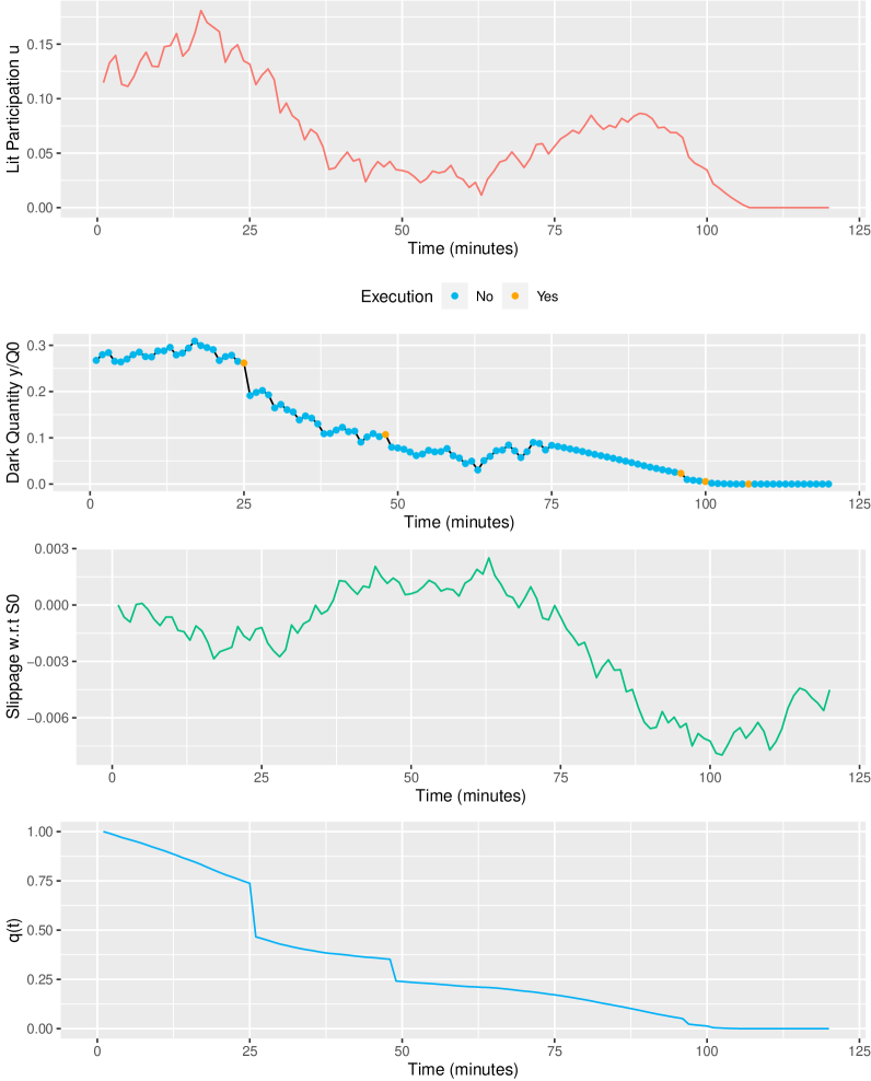
Figure 5: Optimal execution with a lit market and a dark pool

8 Conclusion

We have shown that by adding a mean-reversion signal in the price slippage dynamics, we obtain an optimal execution problem following an LQR specification. The exact shape of the optimal policy function can be iteratively derived before the order starts, and is aggressive in the money. If round-trip trades must be avoided, the MPC approach can impose positivity constraints on the participation curve while remaining close to the LQR optimal strategy. In the continuous trading limit with no permanent impact, we have seen that one can derive a closed formula for the optimal policy which can be further simplified under no urgency, full completion condition, and when the mean-reversion signal is weak. Finally, we have seen that it is possible (although heuristic) to construct a two-step strategy in the presence of an additional dark pool, where a lit MPC policy and a dark LQR strategy work together.

The mean-reversion signal can be seen from different perspectives. It can be an actual, local mean-reversion signal that one has estimated on a particular asset. However, it is often difficult to find reliable patterns in price series. Still, such signals may exist, in particular if the execution task concerns not one but a pair of stocks or more. As exposed in Section 5, another approach consists in using the mean-reverting signal as a tuning parameter in the optimizer to induce a certain level of aggressiveness in the money. This can be motivated by the broker’s inside information or by clients who have their own agenda.

We leave for future research the case of multi-asset optimal execution and rolling MPC as exposed at the end of Section 4. Although they are of great importance for more advanced practical applications, we believe that they are complex problems and they both deserve more than a mere section in the present paper.

9 Appendix

9.1 Proofs of Theorem 1 and Theorem 2

We prove only Theorem 2, since Theorem 1 corresponds to the particular case $\alpha_{t}=0$. Let $\mathcal{I}=\text{diag}(1,1)$, and $\mathcal{J}=\text{diag}(1,0)$. Recall the Bellman equation

$$H(t,X)=\inf_{u\in\mathbb{R}}\left\{j_{t}(X,u)\delta t+\underbrace{\mathbb{E}\left[H\left(t+\delta t,X-\kappa_{t}\delta t\mathcal{J}X+a_{t}w_{t}\delta tu+\left(\begin{matrix}\alpha_{t}\delta t+\sigma_{t,\delta t}z_{t}\\ 0\end{matrix}\right)\right)\right]}_{h_{t}(X,u)}\right\}.$$

We prove our claim on $H(t,X)$ and $u_{t}^{*}$ by descending induction on $t\in\{0,\delta t,...,T\}$. At time $T$, there is no control, and $H(T,X)=\tilde{\beta}_{T}q_{T}^{2}$ which is the claimed quadratic form in $T$, with $P_{T}$, $b_{T}^{T}$ and $e_{T}$ as stated in Theorem 1. Assume now that the claim is true on $t+\delta t,...,T$. Then we have

$$j_{t}(X,u)=a_{t}\eta_{t}u^{2}+a_{t}(p+s_{t})u+\beta_{t}q^{2}$$

and direct calculations using $H(t+\delta t,X)=X^{T}P_{t+\delta t}X+b_{t+\delta t}^{T}X+e_{t+\delta t}$ yield

$$h_{t}(X,u) = a_{t}^{2}\delta t^{2}w_{t}^{T}P_{t+\delta t}w_{t}u^{2}+\left\{2a_{t}\left(X^{T}\left(\mathcal{I}-\kappa_{t}\delta t\mathcal{J}\right)+\alpha_{t}\delta te_{1}^{T}\right)P_{t+\delta t}w_{t}+a_{t}b_{t+\delta t}^{T}w_{t}\right\}\delta tu$$

$$+ X^{T}\left(\mathcal{I}-\kappa_{t}\delta t\mathcal{J}\right)P_{t+\delta t}\left(\mathcal{I}-\kappa_{t}\delta t\mathcal{J}\right)X+\left[b_{t+\delta t}^{T}+2\alpha_{t}\delta te_{1}^{T}P_{t+\delta t}\right]\left(\mathcal{I}-\kappa_{t}\delta t\mathcal{J}\right)X$$

$$+ e_{t+\delta t}+\alpha_{t}\delta tb_{t+\delta t}^{T}e_{1}+\left[\sigma_{t,\delta t}^{2}+\alpha_{t}^{2}(\delta t)^{2}\right]e_{1}^{T}P_{t+\delta t}e_{1}.$$

Hence $j_{t}(X,u)\delta t+h_{t}(X,u)$ is quadratic in $u$ and we readily check that the optimal $u$ which makes it minimal is given by $k_{t}^{T}X+f_{t}$. We then directly get that plugging this is in $j_{t}(X,u)\delta t+h_{t}(X,u)$ yields the quadratic expression in $X$

$$H(t,X)=X^{T}P_{t}X+b_{t}^{T}X+e_{t}$$

with

$$P_{t}=P_{t+\delta t}-\kappa\delta t(\mathcal{J}P_{t+\delta t}+P_{t+\delta t}\mathcal{J})+\kappa^{2}(\delta t)^{2}\mathcal{J}P_{t+\delta t}\mathcal{J}+\left[\Delta_{t}-a_{t}g_{t}k_{t}k_{t}^{T}\right]\delta t,$$

$$b_{t}=b_{t+\delta t}-\left\{2a_{t}g_{t}f_{t}k_{t}+\kappa_{t}\mathcal{J}b_{t+\delta t}-2\alpha_{t}(\mathcal{I}-\kappa_{t}\delta t\mathcal{J})P_{t+\delta t}e_{1}\right\}\delta t,$$

$$e_{t}=e_{t+\delta t}+[\sigma_{t,\delta t}^{2}+\alpha_{t}^{2}(\delta t)^{2}]e_{1}^{T}P_{t+\delta t}e_{1}+\left[\alpha_{t}b_{t+\delta t}^{T}e_{1}-a_{t}g_{t}f_{t}^{2}\right]\delta t$$

as claimed in the theorem.

9.2 Proofs of Theorem 3 and Proposition 1

Proof of theorem 3.

We derive the expression of the quadratic form $C_{t}(u_{t},u_{t+\delta t},...,u_{T-\delta t})$. To do so, it is convenient to first extend the state process $X_{t}=(p_{t},q_{t})^{T}$ to $\tilde{X}_{t}=(p_{t},q_{t},u_{t})^{T}$. At time $0\leq t\leq T$, the stage cost $j_{t}(X_{t},u_{t})\delta t$ can be rewritten as a quadratic form in $\tilde{X}_{t}$. We have

$$j_{t}(\tilde{X}_{t})=\tilde{X}_{t}^{T}M_{t}\tilde{X}_{t}+N_{t}\tilde{X}_{t}$$

where we recall that for $t<T$ we have

$$M_{t}=\left(\begin{matrix}0&0&a_{t}/2\\ 0&\beta_{t}&0\\ a_{t}/2&0&a_{t}\eta_{t}\end{matrix}\right),\text{ and }N_{t}=\left(\begin{matrix}0\\ 0\\ a_{t}s_{t}\end{matrix}\right)$$

and at time $T$

$$M_{T}=\left(\begin{matrix}0&0&0\\ 0&\tilde{\beta}_{T}&0\\ 0&0&0\end{matrix}\right),\text{ and }N_{t}=\left(\begin{matrix}0\\ 0\\ 0\end{matrix}\right).$$

Now, the global cost starting from time $t$ is

$$C_{t}(u_{t},u_{t+\delta t},...,u_{T-\delta t})=\sum_{\tau=t}^{T-\delta t}j_{\tau}(\tilde{X}_{\tau})\delta t+J_{T}(\tilde{X}_{T}).$$

Note the linear representation, under CE,

$$\tilde{X}_{\tau} = \underbrace{\left(\begin{matrix}\pi_{(t+\delta t):(\tau-\delta t)}^{\kappa}v_{t}\mu_{t}\delta t&\pi_{(t+2\delta t):(\tau-\delta t)}^{\kappa}v_{t+\delta t}\mu_{t+\delta t}\delta t&...&v_{\tau-\delta t}\mu_{\tau-\delta t}\delta t&0&0&...\\ -a_{t}\delta t&-a_{t+\delta t}\delta t&...&-a_{\tau-\delta t}\delta t&0&0&...\\ 0&0&...&0&1&0&...\end{matrix}\right)}_{L_{\tau}}u_{t:(T-\delta t)}$$

$$+ \underbrace{\left(\begin{matrix}\pi_{t:(\tau-\delta t)}^{\kappa}p_{t}+\sum_{\theta=t}^{\tau-\delta t}\pi_{\theta:(\tau-\delta t)}^{\kappa}\alpha_{\theta}\delta t\\ q_{t}\\ 0\end{matrix}\right)}_{Y_{\tau}},$$

so that

$$C_{t}(u_{t},u_{t+\delta t},...,u_{T-\delta t}) = u_{t:(T-\delta t)}^{T}\left(\left\{\sum_{\tau=t}^{T-\delta t}L_{\tau}^{T}M_{\tau}L_{\tau}\right\}\delta t+L_{T}^{T}M_{T}L_{T}\right)u_{t:(T-\delta t)}$$

$$+ \left(\left\{\sum_{\tau=t}^{T-\delta t}2Y_{\tau}M_{\tau}L_{\tau}+N_{\tau}L_{\tau}\right\}\delta t+2Y_{T}M_{T}L_{T}+N_{T}L_{T}\right)u_{t:(T-\delta t)}$$

$$+ \textbf{c}_{t},$$

where $\textbf{c}_{t}$ is a constant term, as claimed in the theorem. ∎

Proof of Proposition 1.

Remark that the coefficients $k_{t}^{T}$ and $f_{t}$ do not depend on $\sigma_{t,\delta t}^{2}$ in Theorem 2. Hence they would be unchanged if, all things being equal, $\sigma_{t,\delta t}^{2}$ were set to $0$. Therefore, the LQR solver yields the optimal policy under the certainty equivalent problem. On the other hand, by definition, the MPC solver in the absence of constraints precisely gives the optimal participation rate under CE.

∎

9.3 Proofs of Theorem 4, Theorem 5 and Corollary 1

Proof of Theorem 4.

We look again for a quadratic value function of the form $H(t,X)=X^{T}P_{t}X+b_{t}^{T}X+e_{t}$ and will use the verification theorem to back up our claim. Similarly to the discrete case, plugging $H(t,X)$ in (15) and minimizing the quadratic expression in $u_{t}$ easily yields the expression of the optimal strategy in feedback form

$$u_{t}^{*}=k_{t}^{T}X_{t}+f_{t}.$$

Next, evaluating (15) at point $u_{t}^{*}$ and grouping together quadratic terms in $X$, then linear terms in $X$, and finally the constants respectively give the claimed backward differential equations for $P_{t}$, $b_{t}$, and $e_{t}$. By assumption $P_{t}$ is well-defined, and so are $b_{t}$ and $e_{t}$ which follow first order linear differential equations. Finally, by construction $H$ satisfies Theorem 5.2 in Cartea et al. [2015]. ∎

Proof of Theorem 5 and Corollary 1.

Let us write $P_{t}=(p_{ij,t})_{i,j\in\{1,2\}}$ with $p_{12,t}=p_{21,t}$. Under the assumption of the theorem, note that we have

$$k_{t}=\frac{1}{\eta}\left(p_{12,t}-\frac{1}{2},p_{22,t}\right)^{T}$$

where $p_{12,.}$ and $p_{22,.}$ satisfy the following Riccati equations

$$\partial_{t}p_{12,t}=\kappa p_{12,t}+\frac{a}{\eta}p_{22,t}\left(p_{12,t}-\frac{1}{2}\right)$$

and

$$\partial_{t}p_{22,t}=-\beta+\frac{a}{\eta}p_{22,t}^{2}$$

with terminal conditions $p_{22,T}=\tilde{\beta}_{T}$ and $p_{12,T}=0$. Solving for $p_{22,.}$ first note that we have

$$-\frac{\eta}{a}\frac{\partial_{t}p_{22,t}}{\frac{\eta\beta}{a}-p_{22,t}^{2}}=1$$

so that integrating on both sides on $[t,T]$ and using that $\frac{1}{2\sqrt{\frac{\eta\beta}{a}}}\ln\left(\frac{\sqrt{\frac{\eta\beta}{a}}+p_{22,.}}{\sqrt{\frac{\eta\beta}{a}}-p_{22,.}}\right)$ is a primitive for $\frac{\partial_{t}p_{22,.}}{\frac{\eta\beta}{a}-p_{22,.}^{2}}$, we obtain

$$-\frac{\eta}{a}\left[\ln\left(\frac{\sqrt{\frac{\eta\beta}{a}}+p_{22,T}}{\sqrt{\frac{\eta\beta}{a}}-p_{22,T}}\right)-\ln\left(\frac{\sqrt{\frac{\eta\beta}{a}}+p_{22,t}}{\sqrt{\frac{\eta\beta}{a}}-p_{22,t}}\right)\right]=2(T-t)\sqrt{\frac{\eta\beta}{a}}.$$

Replacing $p_{22,T}$ by $\tilde{\beta}_{T}$ and isolating $p_{22,t}$ in the above equation readily yields the claimed representation. Next, we introduce $y(t)=p_{12,t}-\frac{1}{2}$ and note that we have

$$\partial_{t}y(t)=\left(\kappa+\frac{a}{\eta}p_{22,t}\right)y(t)+\frac{\kappa}{2},\text{ and }y(T)=-\frac{1}{2}.$$

Let $y_{0}$ be the solution to the homogenous equation (without the last term $\kappa/2$) satisfying $y_{0}(T)=1$. Then we have

$$\frac{\partial_{t}y_{0}(t)}{y_{0}(t)}=\kappa+\frac{a}{\eta}p_{22,t}$$

so that integrating on both sides on $[t,T]$ yields again

$$\ln\frac{1}{y_{0}(t)}=\kappa(T-t)-\sqrt{\frac{a\beta}{\eta}}\int_{t}^{T}\frac{\zeta e^{2\sqrt{\frac{a\beta}{\eta}}(T-s)}-1}{\zeta e^{2\sqrt{\frac{a\beta}{\eta}}(T-s)}+1}ds.$$

Using that $\sqrt{\frac{a\beta}{\eta}}\int_{t}^{T}\frac{\zeta e^{2\sqrt{\frac{a\beta}{\eta}}(T-s)}}{\zeta e^{2\sqrt{\frac{a\beta}{\eta}}(T-s)}+1}ds=-\frac{1}{2}\ln\left(\frac{1+\zeta e^{2\sqrt{\frac{a\beta}{\eta}}(T-t)}}{1+\zeta}\right)$ and $-\sqrt{\frac{a\beta}{\eta}}\int_{t}^{T}\frac{1}{\zeta e^{2\sqrt{\frac{a\beta}{\eta}}(T-s)}+1}ds=\frac{1}{2}\ln\left(\frac{\zeta+e^{-2\sqrt{\frac{a\beta}{\eta}}(T-t)}}{1+\zeta}\right)$, and isolating $y_{0}(t)$ yields

$$y_{0}(t)=\frac{1+\zeta}{e^{\left(\kappa-\sqrt{\frac{a\beta}{\eta}}\right)(T-t)}+\zeta e^{\left(\kappa+\sqrt{\frac{a\beta}{\eta}}\right)(T-t)}}.$$

Now, by the variation of constants method, we easily obtain that the solution to the original equation is given by

$$y(t)=\left(-\frac{1}{2}-\frac{\kappa}{2}\int_{t}^{T}y_{0}(s)^{-1}ds\right)y_{0}(t)$$

which gives the claimed value for $p_{12,t}=y(t)+\frac{1}{2}.$ We finally need to show that $f_{t}$ = 0. Let $b_{t}=(b_{1,t},b_{2,t})^{T}$. Then we have $f_{t}=\frac{b_{2,t}}{2\eta}$. Plugging this value into the differential equation for $b_{2,t}$ gives

$$\partial_{t}b_{2,t}=\frac{2a}{\eta}b_{2,t}p_{22,t}$$

with the terminal condition $b_{2,T}=0$. It is immediate to see that $b_{2,t}=0$ is the unique solution to the above Cauchy problem, so that $f_{t}=0$ as well and we are done. The corollary is simply obtained by first taking the pointwise limit $\beta\to 0$ in the above expressions and then by taking $\tilde{\beta}_{T}\to+\infty$. ∎

9.4 Proofs of Theorem 6 and Theorem 7

The following lemma will be convenient for calculations.

Lemma 1.

Let $P\in\mathbb{R}^{2\times 2}$ be a deterministic matrix. Then for $0\leq t\leq T$

$$\mathbb{E}\left[\frac{a_{t}^{2}}{v_{t}^{2}}(\epsilon_{t}^{D})^{2}e_{2}^{T}Pe_{2}\right]=\frac{a_{t}^{2}}{v_{t}^{2}}\lambda_{t}^{D}e_{2}^{T}Pe_{2}\delta t.$$

Proof.

This is a direct consequence of the fact that $\epsilon_{t}^{D}$ follows a Bernoulli distribution with parameter $\lambda_{t}^{D}\delta t$. ∎

Proof of Theorem 6.

Let $0\leq t\leq T$ and $s\geq t$ as in the theorem. Recall that

$$j_{s}^{D}(X^{D},y)=(\delta t)^{-1}\frac{a_{s}}{v_{s}}\theta_{s}^{D}\epsilon_{s}^{D}y^{2}+(\delta t)^{-1}\frac{a_{s}}{v_{s}}\epsilon_{s}^{D}py+\left(\theta_{s}^{D}+(\delta t)^{-1}\frac{\eta_{s}}{v_{s}}\epsilon_{s}^{D}\right)a_{s}\langle u\rangle_{t}y_{s}+\beta_{s}^{D}(q^{D})^{2}.$$

Let

$$h_{s}^{D}(X^{D},y)=\mathbb{E}\left[H^{D}\left(s+\delta t,X^{D}-\kappa_{s}\delta t\mathcal{J}X^{D}-\frac{a_{s}}{v_{s}}\epsilon_{s}^{D}e_{2}y+\left(\begin{matrix}\alpha_{s}\delta t+\sigma_{s,\delta t}z_{s}\\ 0\end{matrix}\right)\right)\right].$$

Similar reasoning to that of the proof of Theorem 1 yields

$$h_{s}^{D}(X,y) = (X^{D})^{T}(\mathcal{I}-\kappa_{s}\delta t\mathcal{J})P_{s+\delta t}^{D}(\mathcal{I}-\kappa_{s}\delta t\mathcal{J})X^{D}$$

$$- 2\frac{a_{s}\lambda_{s}^{D}}{v_{s}}(X^{D})^{T}(\mathcal{I}-\kappa_{s}\delta t\mathcal{J})P_{s+\delta t}^{D}e_{2}y\delta t+2\alpha_{s}\delta te_{1}^{T}P_{s+\delta t}^{D}\left[(\mathcal{I}-\kappa_{s}\delta t\mathcal{J})X^{D}-\frac{a_{s}\lambda_{s}^{D}\delta t}{v_{s}}e_{2}y\right]$$

$$+ a_{s}^{2}\delta t\frac{\lambda_{s}^{D}}{v_{s}^{2}}e_{2}^{T}P_{s+\delta t}^{D}e_{2}y^{2}+(b_{s+\delta t}^{D})^{T}[(\mathcal{I}-\kappa_{s}\delta t\mathcal{J})X^{D}+\alpha_{s}\delta te_{1}]-a_{s}\frac{\lambda_{s}^{D}}{v_{s}}(b_{s+\delta t}^{D})^{T}e_{2}y\delta t$$

$$+ e_{s+\delta t}+\sigma_{s,\delta t}^{2}e_{1}^{T}P_{s+\delta t}^{D}e_{1},$$

hence

$$\mathbb{E}[j_{s}^{D}(X,y)\delta t]+h_{s}^{D}(X,y) = \left[a_{s}\frac{\theta_{s}^{D}\lambda_{s}^{D}}{v_{s}}+\frac{a_{s}^{2}\lambda_{s}^{D}}{v_{s}^{2}}e_{2}^{T}P_{s+\delta t}^{D}e_{2}\right]\delta ty^{2}$$

$$+ \frac{a_{s}}{v_{s}}\lambda_{s}^{D}\bigg{[}(X^{D})^{T}e_{1}-2(X^{D})^{T}(\mathcal{I}-\kappa_{s}\delta t\mathcal{J})P_{s+\delta t}^{D}e_{2}$$

$$- (b_{s+\delta t}^{D})^{T}e_{2}-2\alpha_{s}\delta te_{1}^{T}P_{s+\delta t}^{D}e_{2}+\left(\frac{v_{s}\theta_{s}^{D}}{\lambda_{s}^{D}}+\eta_{s}\right)\langle u\rangle_{t}\bigg{]}y\delta t$$

$$+ (X^{D})^{T}[(\mathcal{I}-\kappa_{s}\delta t\mathcal{J})P_{s+\delta t}^{D}(\mathcal{I}-\kappa_{s}\delta t\mathcal{J})+\Delta_{s}^{D}]X^{D}$$

$$+ (b_{s+\delta t}^{D})^{T}[(\mathcal{I}-\kappa_{s}\delta t\mathcal{J})X^{D}+\alpha_{s}\delta te_{1}]$$

$$+ 2\alpha_{s}\delta te_{1}^{T}P_{s+\delta t}^{D}(\mathcal{I}-\kappa_{s}\delta t\mathcal{J})X^{D}+e_{s+\delta t}^{D}+[\sigma_{s,\delta t}^{2}+\alpha_{s}^{2}(\delta t)^{2}]e_{1}^{T}P_{s+\delta t}^{D}e_{1}$$

where $\Delta_{s}^{D}=\text{diag}[0,\beta_{s}^{D}]$. Letting

$$g_{s}^{D}=\theta_{s}^{D}+\frac{a_{s}}{v_{s}}e_{2}^{T}P_{s+\delta t}^{D}e_{2}$$

$$(k_{s}^{D})^{T}=-(g_{s}^{D})^{-1}\left[-e_{2}^{T}(P_{s+\delta t}^{D})^{T}(\mathcal{I}-\kappa_{s}\delta t\mathcal{J})+\frac{1}{2}e_{1}^{T}\right]$$

and

$$f_{s}^{D}=-\frac{1}{2}(g_{s}^{D})^{-1}\left[-e_{2}^{T}b_{s+\delta t}^{D}-2\alpha_{s}\delta te_{1}^{T}P_{s+\delta t}^{D}e_{2}+\left(\frac{v_{s}\theta_{s}^{D}}{\lambda_{s}^{D}}+\eta_{s}\right)\langle u\rangle_{t}\right]$$

we obtain

$$\mathbb{E}[j_{s}^{D}(X^{D},y)\delta t]+h_{s}(X^{D},y) = \frac{a_{s}\lambda_{s}^{D}}{v_{s}}\delta tg_{s}^{D}y^{2}-2\frac{a_{s}\lambda_{s}^{D}}{v_{s}}\delta t[X^{T}k_{s}^{D}+f_{s}^{D}]g_{s}^{D}y$$

$$+ (X^{D})^{T}[(\mathcal{I}-\kappa_{s}\delta t\mathcal{J})P_{s+\delta t}^{D}(\mathcal{I}-\kappa_{s}\delta t\mathcal{J})+\Delta_{s}^{D}]X^{D}$$

$$+ (b_{s+\delta t}^{D})^{T}(\mathcal{I}-\kappa_{s}\delta t\mathcal{J})X^{D}+e_{s+\delta t}^{D}+[\sigma_{s,\delta t}^{2}+\alpha_{s}^{2}(\delta t)^{2}]e_{1}^{T}P_{s+\delta t}^{D}e_{1}$$

hence the expression of $y_{s}^{*}$ in feedback form

$$y_{s}^{*}=(k_{s}^{D})^{T}X^{D}+f_{s}^{D}.$$

Plugging back $y_{s}^{*}$ into the expression above yields

$$P_{s}^{D}=P_{s+\delta t}^{D}-\kappa_{s}\delta t(\mathcal{J}P_{s+\delta t}^{D}+P_{s+\delta t}^{D}\mathcal{J})+\kappa_{s}^{2}(\delta t)^{2}\mathcal{J}P_{s+\delta t}^{D}\mathcal{J}+\left[\Delta_{s}-\frac{a_{s}\lambda_{s}^{D}}{v_{s}}g_{s}^{D}k_{s}^{D}(k_{s}^{D})^{T}\right]\delta t,$$

$$b_{s}^{D}=b_{s+\delta t}^{D}-\left\{2\frac{a_{s}\lambda_{s}^{D}}{v_{s}}g_{s}^{D}f_{s}^{D}k_{s}^{D}+\kappa_{s}\mathcal{J}b_{s+\delta t}-2\alpha_{s}(\mathcal{I}-\kappa_{s}\delta t\mathcal{J})P_{s+\delta t}^{D}e_{1}\right\}\delta t,$$

$$e_{s}^{D}=e_{s+\delta t}^{D}+[\sigma_{s,\delta s}^{2}+\alpha_{s}^{2}(\delta t)^{2}]e_{1}^{T}P_{s+\delta t}^{D}e_{1}+\left[\alpha_{s}(b_{s+\delta t}^{D})^{T}e_{1}-\frac{a_{s}\lambda_{s}^{D}}{v_{s}}g_{s}^{D}(f_{s}^{D})^{2}\right]\delta t$$

as claimed in the theorem.

∎

Proof of Theorem 7.

This follows the same line of reasoning as for the proof of Theorem 4. ∎

References

• Alessio and Bemporad [2009] Alessandro Alessio and Alberto Bemporad. A survey on explicit model predictive control. In Nonlinear model predictive control, pages 345–369. Springer, 2009.
• Alfonsi and Blanc [2016] Aurélien Alfonsi and Pierre Blanc. Dynamic optimal execution in a mixed-market-impact hawkes price model. Finance and Stochastics, 20(1):183–218, 2016.
• Almgren and Chriss [2001] Robert Almgren and Neil Chriss. Optimal execution of portfolio transactions. Journal of Risk, 3:5–40, 2001.
• Bemporad and Filippi [2003] Alberto Bemporad and Carlo Filippi. Suboptimal explicit receding horizon control via approximate multiparametric quadratic programming. Journal of optimization theory and applications, 117(1):9–38, 2003.
• Bemporad et al. [2002] Alberto Bemporad, Manfred Morari, Vivek Dua, and Efstratios N Pistikopoulos. The explicit linear quadratic regulator for constrained systems. Automatica, 38(1):3–20, 2002.
• Bertsekas et al. [1995] Dimitri P Bertsekas, Dimitri P Bertsekas, Dimitri P Bertsekas, and Dimitri P Bertsekas. Dynamic programming and optimal control, volume 1. Athena scientific Belmont, MA, 1995.
• Bertsimas and Lo [1998] Dimitris Bertsimas and Andrew W Lo. Optimal control of execution costs. Journal of Financial Markets, 1(1):1–50, 1998.
• Busseti and Boyd [2015] Enzo Busseti and Stephen Boyd. Volume weighted average price optimal execution. arXiv preprint arXiv:1509.08503, 2015.
• Cartea et al. [2015] Álvaro Cartea, Sebastian Jaimungal, and José Penalva. Algorithmic and high-frequency trading. Cambridge University Press, 2015.
• Cutler and Ramaker [1980] Charles R Cutler and Brian L Ramaker. Dynamic matrix control - a computer control algorithm. In joint automatic control conference, number 17, page 72, 1980.
• Garcia et al. [1989] Carlos E Garcia, David M Prett, and Manfred Morari. Model predictive control: theory and practice—a survey. Automatica, 25(3):335–348, 1989.
• Gatheral and Schied [2011] Jim Gatheral and Alexander Schied. Optimal trade execution under geometric brownian motion in the almgren and chriss framework. International Journal of Theoretical and Applied Finance, 14(03):353–368, 2011.
• Guéant [2016] Olivier Guéant. The Financial Mathematics of Market Liquidity: From optimal execution to market making, volume 33. CRC Press, 2016.
• Guéant and Royer [2014] Olivier Guéant and Guillaume Royer. Vwap execution and guaranteed vwap. SIAM Journal on Financial Mathematics, 5(1):445–471, 2014.
• Hora [2006] Merell Hora. Tactical liquidity trading and intraday volume. Preprint, 2006.
• Huberman and Stanzl [2004] Gur Huberman and Werner Stanzl. Price manipulation and quasi-arbitrage. Econometrica, 72(4):1247–1275, 2004.
• Huberman and Stanzl [2005] Gur Huberman and Werner Stanzl. Optimal liquidity trading. Review of Finance, 9(2):165–200, 2005.
• Li et al. [2014] Zhijun Li, Yuanqing Xia, Chun-Yi Su, Jun Deng, Jun Fu, and Wei He. Missile guidance law based on robust model predictive control using neural-network optimization. IEEE transactions on neural networks and learning systems, 26(8):1803–1809, 2014.
• Martin et al. [1986] GD Martin, JM Caldwell, and TE Ayral. Predictive control applications for the petroleum refining industry. In Petroleum Refining Conference, Tokyo, Japan, 1986.
• Morari and Lee [1999] Manfred Morari and Jay H Lee. Model predictive control: past, present and future. Computers & Chemical Engineering, 23(4-5):667–682, 1999.
• Obizhaeva and Wang [2013] Anna A Obizhaeva and Jiang Wang. Optimal trading strategy and supply/demand dynamics. Journal of Financial Markets, 16(1):1–32, 2013.
• Qin and Badgwell [2003] S Joe Qin and Thomas A Badgwell. A survey of industrial model predictive control technology. Control engineering practice, 11(7):733–764, 2003.
• Richalet et al. [1978] Jacques Richalet, André Rault, JL Testud, and J Papon. Model predictive heuristic control. Automatica (journal of IFAC), 14(5):413–428, 1978.
• Schied et al. [2010] Alexander Schied, Torsten Schöneborn, and Michael Tehranchi. Optimal basket liquidation for cara investors is deterministic. Applied Mathematical Finance, 17(6):471–489, 2010.
• Shen [2017] Jackie Shen. Hybrid is-vwap dynamic algorithmic trading via lqr. Available at SSRN 2984297, 2017.