Interpretable Machine Learning for Resource Allocation with Application to Ventilator Triage

Abstract

Rationing of healthcare resources is a challenging decision that policy makers and providers may be forced to make during a pandemic, natural disaster, or mass casualty event. Well-defined guidelines to triage scarce life-saving resources must be designed to promote transparency, trust and consistency. To facilitate buy-in and use during high stress situations, these guidelines need to be interpretable and operational. We propose a novel data-driven model to compute interpretable triage guidelines based on policies for Markov Decision Process that can be represented as simple sequences of decision trees (tree policies). In particular, we characterize the properties of optimal tree policies and present an algorithm based on dynamic programming recursions to compute good tree policies. We utilize this methodology to obtain simple, novel triage guidelines for ventilator allocations for COVID-19 patients, based on real patient data from Montefiore hospitals. We also compare the performance of our guidelines to the official New York State guidelines that were developed in 2015 (well before the COVID-19 pandemic). Our empirical study shows that the number of excess deaths associated with ventilator shortages could be reduced significantly using our policy. Our work highlights the limitations of the existing official triage guidelines, which need to be adapted specifically to COVID-19 before being successfully deployed.

Keywords: Triage guidelines, SARS-CoV-2, New York State Guidelines, Interpretable Machine Learning, Markov Decision Process

1 Introduction

Healthcare delivery operates in a resource limited environment where demand can sometimes exceed supply, resulting in situations where providers have to make difficult decisions of who to prioritize to receive scarce resources. Having a framework to guide such decisions is critical, particularly with growing threats of pandemics, natural disasters, and mass casualty events that make the healthcare system vulnerable to situation where demand vastly exceeds supply of critical healthcare resources. Triage of health resources in such situations has garnered quite a bit of attention from the Operations Management (OM) community (Jacobson et al. 2012, Mills et al. 2013, Sun et al. 2018). The primary focus of prior work has been to determine how care should be rationed. In this work, we develop a machine learning methodology that considers how data can be used to guide these decisions in an interpretable manner and what criteria should be considered in these life-or-death decisions.

Triage guidelines are often implemented during high stress, complex situations. As such, triage algorithms need to be systematic, simple and intuitive in order to facilitate adoption and to ease the decision burden on the provider. In 2012, the National Academy of Medicine identified an ethical framework for triage (Gostin et al. 2012). In this framework, the primary component which the operations community has focused on is ‘the duty to steward resources’, which calls for withholding or withdrawing resources from patients who will not benefit from them. In this work, we take a data-driven approach to develop triage guidelines for ventilator allocation in order to maximize lives saved. Such decisions are ethically challenging and such an objective can sometimes be in tension with other critical elements such as fairness. We will also examine how the ethics and fairness criteria can be incorporated into such decisions.

On the one hand, government officials have issued pre-specified and transparent utilitarian triage guidelines for preventing loss of life, promote fairness, and support front-line clinicians (Christian et al. 2014, Zucker et al. 2015, Piscitello et al. 2020). In the United States, 26 states have scarce resource allocation guidelines  (Babar and Rinker 2016). These guidelines emphasize simplicity, and can often be represented as decision trees of small depth (Breiman et al. 1984, Bertsimas and Dunn 2017). However, these guidelines have never been used in practice, and are not constructed in a data-driven way, but rather via expert opinion of clinicians, policy makers, and ethicists. Therefore, it is not known how well they perform for the intended purpose of directing scarce resources to those most likely to benefit. In addition, we cannot ethically perform a prospective study to determine the efficacy (or performance) of such policies.

On the other hand, there is a large body of literature in the OM community on the management of healthcare resources, including breast magnetic resonance imaging (Hwang and Bedrosian 2014), patient scheduling (Bakker and Tsui 2017), ICU beds (Chan et al. 2012, Kim et al. 2015), mechanical ventilators and high-flow nasal cannula (Gershengorn et al. 2021, Anderson et al. 2021). Because the health of each patient evolves dynamically over time, the problem of scarce resource allocation is inherently sequential in nature. In theory, one can leverage the tools from OM and Machine Learning (ML) to compute new allocation guidelines. Markov Decision Processes (MDPs) and queueing theory are tools that are commonly used to find optimal sequences of decisions in a stochastic environment (Puterman 1994, Whitt 2002). With such methodologies, optimal policies can often be numerically computed efficiently using iterative algorithms; however, the optimal policies may not have an interpretable structure. This is often referred to as black-box policies in the ML community (Rudin 2019). To obtain practical operational guidelines, it is necessary to obtain interpretable decision rules that can easily be explained and implemented by the medical staff and discussed with the practitioners. This becomes even more important for the ethically challenging task of triaging scarce life-sustaining resources. In this case, what constitutes an appropriate input into the model may be contested. For instance, age is a strong predictor of outcomes for patients infected with Sars-CoV-2, but ethicists disagree about the appropriateness of using age in triage decisions (May and Aulisio 2020). For triage algorithms to be used in practice, triage rules must be exposed for public debate, and therefore, interpretability is a key property.

In certain settings, simple index-based triage rules can be shown to perform well (e.g. , the $c\mu$-rule for multiclass queues with Poisson arrivals (Van Mieghem 1995). However, these works typically assume static patient health status and/or a limited number of patient classes (e.g. two classes in Van Mieghem (1995)). The complexity of these problems arises from the capacity constraint which creates externalities across different patients. In contrast, we consider a setting where the health status of each patient evolves dynamically (and stochastically) overtime. This richer state-space for the patient state substantially increases the computational complexity of our model and renders existing approaches for triage intractable. As such, we develop a model that explicitly incorporates the dynamic patient health state and approximates the capacity constraint through appropriately calibrated cost parameters.

Our goal in this paper is to develop allocation guidelines that are both data-driven and interpretable. To do so, we propose a new model for interpretable sequential decision-making, based on decision trees. We then apply this methodology to develop guidelines for ventilator allocation for COVID-19 patients. The COVID-19 pandemic has highlighted the challenge of managing life-saving health resources as demand for intensive care unit beds, critical appliances such as mechanical ventilators, and therapies such as dialysis all were in short supply in many countries. Shortages of ventilators and oxygen have occurred in Italy and India, amongst other countries (Rosenbaum 2020, Kotnala et al. 2021). Given the ongoing risks of emerging infectious diseases (Zumla et al. 2016) and the projected increase in frequency of extreme weather events (Woodward and Samet 2018), hospitals are increasingly vulnerable to conditions that may result in periods of scarcity of life-sustaining resources even after the COVID-19 pandemic subsides. We utilize the question of ventilator allocation for COVID-19 patients as a canonical example of how our methodology can be used to develop data-driven, interpretable triage guidelines for such settings.

Our main contributions can be summarized as follows:

• Interpretable policies for MDPs. We propose a framework to derive interpretable decision rules with good performances for sequential decision-making problems, based on decision trees. In particular, we model the evolution of the health of the patient as an MDP and we focus on tree policies, which have a tree-like structure, and provide intuitive and explainable decision rules for MDPs. We highlight the challenges of computing optimal tree policies by showing that this problem is a generalization of computing optimal classification trees, which is known to be NP-hard.

• Properties of optimal tree policies. By construction, the set of policies we consider is constrained to have a tree-like structure. Therefore, the properties of optimal tree policies are in stark contrast with the classical properties for unconstrained MDPs. We show that optimal tree policies may depend on the initial condition, and may even be history-dependent. However, we show that an optimal tree policy can be chosen to be deterministic. Therefore, we propose an adaption of value iteration, a classical algorithm which returns an unconstrained, Markovian policy, to ensure the resulting policy is a tree policy. We also show that an optimal tree policy can always be chosen to be deterministic (though it may be history-dependent).

• Algorithm for tree policies. We develop an algorithm for computing a tree policy. Since computing history-dependent policies may be intractable, we focus on finding Markovian tree policies. Our algorithm performs dynamic programming recursions akin to Bellman recursions but forces the visited policies to be tree policies.

• Application to mechanical ventilators allocations. We apply our novel model and algorithm to compute interpretable triage guidelines for ventilator allocations for COVID-19 patients. We leverage a data set of 807 COVID-19 patients intubated at an urban academic medical center in New York City and build an MDP model to obtain interpretable triage guidelines. We compare them to the official New York State (NYS) guidelines and First-Come-First-Served (FCFS) guidelines. We find that our proposed tree policy may lead to up to a $25\%$ decrease in excess deaths, compared to the NYS and FCFS rules. Compared to NYS guidelines, our novel triage policy is less aggressive and exclude less patients.

Outline. This rest of this paper is organized as follows. The end of this section is devoted to a brief literature review. In Section 2, we introduce our Markov Decision Process (MDP) model. In Section 3, we introduce our tree policies for MDPs, we present the properties of optimal tree policies and we present our algorithm to compute good tree policies. In Section 4, we present our numerical study (data set, MDP model, simulation model), applying our framework to mechanical ventilator allocations for COVID-19 patients. We discuss our empirical results in Section 5, where we detail our comparison of various triage guidelines under different levels of ventilator shortages.

1.1 Related literature

Our work primarily builds upon (i) triage guidelines for scarce healthcare resources, (ii) decision trees and MDPs for decision making in healthcare, and (iii) recent advances to compute interpretable decisions in sequential decision-making.

Triage guidelines in the Operations Management literature. There is a large body of literature in the operations management (OM) and medical literature on designing efficient triage guidelines for allocations of scarce healthcare resources. In a broad sense, the usual objective is of doing the greatest good for the greatest number (Frykberg 2005). For instance, Sacco et al. (2007) proposes to use linear programming to determine priorities among patients in the hospitals, and Jacobson et al. (2012) rely on sample-path methods and stochastic programming for computing policies for assignments to key resources (such as ambulances and operating rooms) in the aftermath of mass-casualty events. Kim et al. (2015) estimates the impact of ICU admission denials on the outcomes of the patients. Triage conditions can be tailored to various situations, including austere conditions and imperfect information (Argon and Ziya 2009, Childers et al. 2009, Li and Glazebrook 2010, Sun et al. 2018) or specific health conditions, such as burn-injured patients (Chan et al. 2013). Note that triage guidelines are also of interest in other area of OM, e.g. allocating customers to servers (Dobson and Sainathan 2011, Alizamir et al. 2013). Other works analyze directly the regimes where triage may or may not be beneficial (Sun et al. 2019), and the impact of available capacity on triage decisions (Chen et al. 2020). Perhaps most similar to our paper is the work in Anderson et al. (2021). The authors also look at the NYS ventilator allocation guidelines and compare to two guidelines they developed which incorporate machine learning predictors (regularized logistic regressions) beyond just the Sequential Organ Failure Assessment (SOFA) score. We take a different methodological approach. While Anderson et al. (2021) focus on the prediction of survivability and length-of-ventilation, we develop a methodology to identify a tree-based policy to allocate ventilators, emphasizing the interpretability of our decision guidelines. More generally, the efficiency of the triage guidelines are often demonstrated numerically and, in some instances, some structural properties of optimal policies can be derived theoretically. Many of these works focus on index policies in order to facilitate implementation, even if the optimal policy is quite complex. The indices are often derived from aggregate metrics which capture factors like survival risk, length-of-stay, and/or risk of mis-triage. However, such approaches can obscure clinical features resulting in lack of interpretability and are not easily explainable to the medical staff.

Decision trees and MDPs in healthcare. Tree-based models are popular in general classification tasks, and specifically in healthcare applications. Indeed, they provide a decision model that often achieves high classification accuracy based on simple decision rules. Classical heuristics such as CART (Breiman et al. 1984) and C4.5 (Quinlan 2014) scale well but often return suboptimal trees, while optimal solutions can be computed with integer programming (Bertsimas and Dunn 2017). In healthcare, decision trees have been used in a number of settings including diagnosing heart diseases (Shouman et al. 2011), developing novel non-linear stroke risk scores (Orfanoudaki et al. 2020), and predicting survival probability of the patients (Bertsimas et al. 2020). As the scope of applications of decision trees to healthcare decision-making is very large, we refer the reader to the reviews in Tomar and Agarwal (2013) and Dhillon and Singh (2019). Most of these applications are based on static predictions (e.g., diagnosis) of the diseases and do not take into account the dynamic evolution of the health of the patient over time. In contrast, we build upon the Markov Decision Process (MDP) literature to better model the impact of our decisions over time.

Markov Decision Processes (MDPs) provide a simple framework for the analysis of sequential decision rules. This is the reason why MDPs are widely used in many healthcare applications, where the evolution of the patient’s health impacts the sequence of decisions chosen over time. The use of Markov models in healthcare can be traced back to Beck and Pauker (1983). In particular, MDPs have been used, among others, for kidney transplantation (Alagoz et al. 2004), HIV treatment recommendations (Shechter et al. 2008), cardiovascular controls for patients with Type 2 diabetes (Steimle and Denton 2017) and determining proactive transfer policies to the ICU (Grand-Clément et al. 2020). We refer the reader to Alagoz et al. (2010) for reviews of applications of MDP to healthcare.

Interpretable sequential decision-making. Decision trees are efficient where there is a single decision epoch. This is the setting where there has been the most traction of interpretable machine learning in healthcare settings (Khan et al. 2008, Amin and Ali 2018, Bertsimas et al. 2020). In contrast, MDPs are suitable for modeling sequential decisions but do not, a priori, incorporate interpretability constraints. Recently, there has been some works toward developing methods for interpretable policies in sequential decision-making(not necessarily specific to the healthcare setting). Bravo and Shaposhnik (2020) propose to explain the optimal unconstrained policies with decision trees, applying their framework to classical operations problems such as queuing control and multi-armed bandit (MAB). However, this may be misleading, as there is no guarantee that the novel explainable, suboptimal policies have the same performance as the unconstrained, optimal policies (Rudin 2019). Ciocan and Mišić (2020) introduce the notion of tree policies for stopping time problems and design an algorithm returning an interpretable stopping policy. Their algorithm builds upon top-down approaches for computing classification trees given a data set of observations and labels. Note that the set of actions for a stopping time problem is $\{$go, stop$\}$. In contrast, we focus on MDPs where the set of actions can be any finite set. Additionally, we characterize the theoretical properties of optimal tree policies, which may be history-dependent but can always be chosen to be deterministic. Finally, our algorithmic framework is also different from Ciocan and Mišić (2020). In particular, Ciocan and Mišić (2020) modifies an algorithm for computing classification trees (CART, from Breiman et al. (1984)) to compute stopping time policies. In contrast, we modify an algorithm for computing MDP policies (value iteration) by exploiting an algorithm for classification trees as a subroutine at every iteration (see Algorithm 1), to force value iteration to only visit tree policies. Our overall algorithm is independent of the subroutine used to compute decision trees, and heuristics or optimal methods can be chosen, depending of the preference for fast computations or accuracy of the decision trees returned.

2 Model of sequential decisions

Our goal is to develop guidelines for determining which patients to allocate (or not) a healthcare resource. We consider the dynamic evolution of patient health and how to utilize this information in making triage decisions. We consider a finite-horizon Markov Decision Process (MDP) to model the patient health evolution and we develop a methodology to compute policies, which admit simple tree representations at every decision epoch. In Section 4, we will examine the application of our methodology to ventilator allocations for COVID-19 patients.

We consider a fairly general setting of sequential resource allocation in healthcare. Patient health evolves stochastically over time. We consider the allocation of a single type of healthcare resource (e.g., ICU beds, mechanical ventilator, specialized nurses, medications) to different patients. The nature of the allocation guideline is sequential; the decision can be revisited multiple times and can depend on: 1) the current resource capacity, 2) the current health condition of the focal patient and its potential subsequent improvement and deterioration, and 3) the current health conditions of all other patients and their potential subsequent improvements and deteriorations. Because of the capacity constraint, the decision of allocating a resource (as well as how much) to a single patient impacts the ability to treat other current and, possibly, future patients. While most prior works reduce the state-space by restricting to two classes of patients and/or ignoring the evolution of patient health, the richer model of patient health is an important component of our data-driven approach to triage.

2.1 Evolution of Patient Health and Action Space

We model the health condition of each patient according to a finite-state Markov Chain. We let $s_{t}\in\mathbb{S}_{t}$ denote the health state of a patient in period $t$. Each state represents the health condition which may include information such as vital signs and lab values, as well as comorbidities and demographics. In our specific application to mechanical ventilator allocation we will consider multi-dimensional states, but our model allows for more general, arbitrary (finite) set of states. The vector $\bm{p}_{1}$ represents the likelihood to start in each state in $\mathbb{S}_{1}$. In contrast to the existing OM triage literature, we allow for an arbitrary (finite) number of patient health states that evolve stochastically depending on the action taken.

At each period $t$, let $\mathbb{A}_{t}$ denote the set of discrete possible actions. For example, one could consider a binary decision of whether to intubate or extubate a patient when considering ventilator allocations. Alternatively, one could consider different levels of drug dosages – $\{\sf 100mg,200mg,300mg\}$ – for medication allocation. Once an action $a_{t}$ is chosen based on a policy, the patient transitions to the next state $s_{t+1}\in\mathbb{S}_{t+1}$ with probability $P_{s_{t}a_{t}s_{t+1}}$. The transitions represent the health evolution of the patient toward future states. We assume that the transitions are Markovian to keep the model tractable. Terminal states in $\mathbb{S}_{H}$ represent the status at discharge, typically in the set $\{{\sf deceased,alive}\}$. For conciseness, we assume that the set of states $\mathbb{S}_{1},...,\mathbb{S}_{H}$ attainable at period $t=1,...,H$, are disjoint. This allows use to consider transition kernels and costs that do not depend of the current period.

2.2 Capacity Constraint

Explicitly modeling both the complex patient health evolution over time and the capacity constraint of the shared resource leads to a high-dimensional MDP formulation, which is intractable. When considering the multi-patient allocation problem, a common assumption is that the dynamics of the patients are independent: they are only linked by the utilization of the common resource. This can be seen as a form of weakly coupled processes (Adelman and Mersereau 2008), and a relaxation of this multi-patients allocation problem can be obtained as a classical Markov Decision Process (MDP), describing the health evolution and resource allocation to a single patient, with adequate penalization of the costs vectors. As such, to facilitate some tractability to derive interpretable policies, we consider the allocation for an individual patient and implicitly incorporate the capacity constraint via appropriately defined cost parameters. In particular, in each period $t$, a cost $c_{s_{t}a_{t}}$ reflects the cost incurred given the patient health state $s_{t}$ and action taken $a_{t}$. Intuitively, one would expect that the cost is non-decreasing in the amount of resources allocated to the patient.

The cost parameters reflect the (potentially multiple) objective(s) of the decision maker and can incorporate 1) patient risk of bad outcomes, 2) costs of using healthcare resources (both explicit as well as opportunity costs), and 3) potential risks associated with the action (e.g., complications). The costs can be increased to deter the decision maker from using too much resources compared to a model without any capacity constraint. More rigorously, Adelman and Mersereau (2008) show that the Lagrangian relaxation of a weakly coupled multi-agent decision process results in a single-agent decision process with costs augmented by a factor proportional to the Lagrange multiplier.

While our model ultimately focuses on a single patient with dynamic health state and accounts for the capacity constraint via the cost formulation, we note that the focus on a single patient is the standard approach in designing triage algorithms in the medical community. In particular, the majority of triage guidelines are myopic, and they are only executed when the capacity constraint is met. When there are any available resources, resources are allocated myopically (i.e., to patients that require them) without concern about the future potential of running out of capacity (Zucker et al. 2015, White and Lo 2020).

2.3 Objective function and decision rule

The goal of the decision maker is to minimize the expected cost $C(\pi)$ associated with a policy $\pi=\left(\pi_{1},...,\pi_{H}\right)$, which is a sequence of decision rules $\pi_{t}$ over a finite horizon $H$. Each decision rule $\pi_{t}$ maps a history up to period t, $h_{t}=(s_{1},a_{1},...,s_{t-1},a_{t-1},s_{t})$, to a distribution over the possible actions in $\mathbb{A}_{t}$. The cumulative expected cost associated with a policy $\pi$, $C(\pi)$, is calibrated to capture the balance between clinical objectives (e.g., optimizing survival of the patient) and costs of using resources. It is defined as

$$C(\pi)=\mathbb{E}^{\pi,\bm{P}}\left[\sum_{t=1}^{H}c_{s_{t}a_{t}}\;\bigg{|}\;s_{1}\sim\bm{p}_{1}\right].$$ (2.1)

For a fixed Markovian policy $\pi$, we can associate a collection of value functions $\left(\bm{v}_{t}^{\pi}\right)_{t\in[H]}\in\mathbb{R}^{\mathbb{S}_{1}\times....\times\mathbb{S}_{H}}$, defined recursively as

$$v^{\pi}_{H,s} =\sum_{a\in\mathbb{A}_{H}}\pi_{H,sa}c_{H,sa},\forall\;s\in\mathbb{S}_{H},$$

$$v^{\pi}_{t,s} =\sum_{a\in\mathbb{A}_{t}}\pi_{t,sa}\left(c_{sa}+\sum_{s^{\prime}\in\mathbb{S}_{t+1}}P_{sas^{\prime}}v^{\pi}_{t+1,s^{\prime}}\right),\forall\;s\in\mathbb{S}_{t},\forall\;t\in[H-1].$$

For each period $t\in[H]$ and state $s\in\mathbb{S}_{t}$, $v^{\pi}_{t,s}$ represents the cumulative expected cost from period $t$ to period $H$, starting from state $s$:

$$v^{\pi}_{t,s}=\mathbb{E}^{\pi,\bm{P}}\left[\sum_{t^{\prime}=t}^{H}c_{s_{t^{\prime}}a_{t^{\prime}}}\;\bigg{|}\;s_{t}=s\right].$$

From the definition of the cost $C(\pi)$ as in (2.1), we have $C(\pi)=\bm{p}_{1}^{\top}\bm{v}^{\pi}_{1}$. Crucially, an optimal policy $\pi^{*}$ which minimizes the expected cost (2.1) can be chosen to be Markovian ($\pi^{*}_{t}$ only depends of the current state $s_{t}$ and not of the whole history $h_{t}$), and deterministic (for each state $s_{t}$, $\pi^{*}_{t}$ chooses a degenerate distribution over $\mathbb{A}_{t}$ with weight $1$ on one action and $0$ everywhere). Additionally, $\pi^{*}$ can be computed using the following value iteration algorithm (Puterman 1994): the value functions $\left(\bm{v}_{t}^{*}\right)_{t\in[T]}\in\mathbb{R}^{\mathbb{S}_{1}\times....\times\mathbb{S}_{H}}$ of an optimal policy $\pi^{*}$ follow the Bellman optimality equation (2.2):

$$v^{*}_{H,s} =\min_{a\in\mathbb{A}_{H}}c_{H,sa},\forall\;s\in\mathbb{S}_{H},$$ (2.2)

$$v^{*}_{t,s} =\min_{a\in\mathbb{A}_{t}}c_{sa}+\sum_{s^{\prime}\in\mathbb{S}_{t+1}}P_{sas^{\prime}}v^{*}_{t+1,s^{\prime}},\forall\;s\in\mathbb{S}_{t},\forall t\in[H-1],$$

and an optimal policy $\pi^{*}$ can be chosen as the policy that maps each state $s\in\mathbb{S}_{t}$ to the action attaining the $\arg\min$ in the Bellman equations (2.2).

3 Interpretable Policies

In a healthcare setting, interpretability of the decisions is crucial to operationalize the guidelines and facilitate practical implementation of the policies, generate buy-in from policy makers and providers, and mitigate obscuring of any potential ethical issues. A priori, the optimal policy for a classical, unconstrained MDP instance may not have any interpretable structure. In this work, we use a model of interpretable decisions based on decision trees (Breiman et al. 1984). Intuitively, the goal is to compute an efficient policy for the finite-horizon MDP problem, which can be succinctly represented as an interpretable decision tree at each decision period.

3.1 Classification trees

We start with a brief introduction to decision trees. Decision trees are widely used in classification problems (Breiman et al. 1984, Bertsimas and Dunn 2017). We use the following definition of a decision tree and present two examples of decision trees in $\mathbb{R}^{3}$ in Figure 1.

Definition 3.1.

Let $\mathcal{D}$ be a set of $m$ data points $(\bm{x}_{i},y_{i})$ where $\bm{x}_{i}\in\mathbb{R}^{p}$ are observations and $y_{i}$ are labels in $\mathcal{L}$, where $\mathcal{L}$ is a finite subset of $\mathbb{N}$. A classification tree $T$ is a map $\mathbb{R}^{p}\rightarrow\{1,...,K\}$, with $K\in\mathbb{N}$, which recursively partitions $\mathbb{R}^{p}$ into $K$ disjoint sub-regions (called classes), using branch nodes and leaf nodes. Branch nodes rely on univariate splits such as $x_{1}\leq 2$ or $x_{3}\leq 8$. The point $i$ follows the left branch if it satisfies the splitting condition, otherwise it follows the right branch. Each leaf defines a sub-region of $\mathbb{R}^{p}$, resulting from the sequence of splits leading to this leaf. Each sub-region is uniquely identified with a class $c\in[K]$. Each class $c$ is then mapped to a probability distribution $\bm{\mu}_{c}\in\Delta(\mathcal{L})$ over the set of labels. The scalar $\mu_{cy}$ represents the probability that points belonging to the class $c$ are assigned label $y\in\mathcal{L}$.

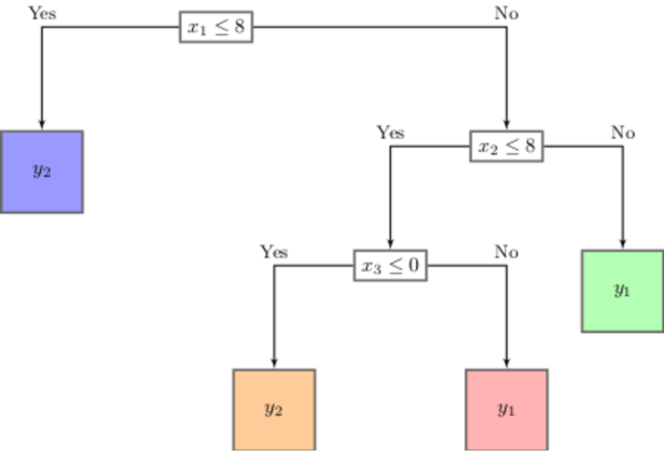
(a) Deterministic tree.

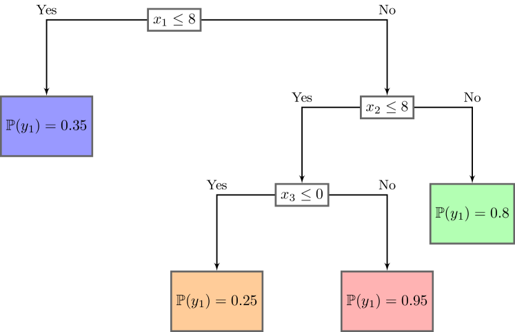
(b) Randomized tree.

Figure 1: Example of two decision trees with three branching nodes, four classes (indicated by the four colors at the leaves) and two labels $y_{1},y_{2}$. The tree in Figure 1(a) is deterministic: at each class, a unique label ($y_{1}$ or $y_{2}$) is assigned. The tree in Figure 1(b) is randomized: at each class, a probability distribution over $\{y_{1},y_{2}\}$ is assigned. Since there are only two labels, we only show $\mathbb{P}(y_{1})$ at each leaf.

We write $\mathcal{T}(\mathcal{X},[K],\mathcal{L})$ as the set of decision trees defining $K$ sub-regions of the set $\mathcal{X}\subset\mathbb{R}^{p}$ and mapping these sub-regions to labels in $\mathcal{L}$. We write $C_{\sf tree}(T)$ the expected weighted classification error of $T$:

$$C_{\sf tree}(T)=\sum_{c=1}^{K}\sum_{i=1}^{m}\sum_{\ell\in\mathcal{L}}\omega_{i,\ell}1_{\{T(\bm{x}_{i})=c\}}\mu_{c\ell},$$ (3.1)

where $\left(\omega_{i,\ell}\right)_{i,\ell}$ are the weights associated with classifying observation $\bm{x}_{i}$ with a label of $\ell\in\mathcal{L}$. Typically, $C_{\sf tree}(T)$ simply counts the expected number of misclassified data points and $\omega_{i,\ell}=0$ if and only if $\ell=y_{i}$, otherwise $\omega_{i,\ell}=1$. Note the bilinear terms $1_{\{T(\bm{x}_{i})=c\}}\mu_{c\ell}$ in the definition (3.1) of $C_{\sf tree}(T)$; $C_{\sf tree}(T)$ can be expressed as a linear objective using standard reformulation techniques (see Appendix A). The Classification Tree (CT) optimization problem is to compute a classification tree which minimizes the expected classification error (3.1):

$$\min \;C_{\sf tree}(T)$$ (CT)

$$T\in\mathcal{T}(\mathcal{X},[K],\mathcal{L})$$

Classical heuristics for (CT) such as CART (Breiman et al. 1984) scale well but often return suboptimal trees. Optimal classification trees can be computed using reformulations as Mixed-Integer Linear Programming (Bertsimas and Dunn 2017). A certain number of interpretability constraints can be incorporated in the set $\mathcal{T}(\mathcal{X},[K],\mathcal{L})$, including upper bounding the depth of the tree, defined as the maximum number of splits leading to a sub-region. Smaller trees are easier to understand as they can be drawn entirely and prevent over-fitting (Bertsimas and Dunn 2017).

3.2 Tree policies for Markov Decision Processes

Decision trees are a popular framework for finding interpretable classification rules, but are not a priori suitable for sequential decision-making. We develop an analogous notion of decision trees for MDPs, which we refer to as tree policies. Intuitively, a policy $\pi$ is called a tree policy if at every period $t$, the decision rule $\pi_{t}$ can be represented as a decision tree which assigns labels (actions, or treatments) from $\mathbb{A}_{t}$ to observations (states, or health conditions) from $\mathbb{S}_{t}$. In particular, we have the following definition. Recall that from our definition of a decision tree in Section 3.1, we see a tree $T$ as a map from the set of observations in $\mathbb{R}^{p}$ to a label in $\{1,...,K\}$, i.e., we have $T:\mathbb{R}^{p}\rightarrow\{1,...,\}$.

Definition 3.2.

Let $\mathcal{M}=(H,\mathbb{S},\mathbb{A},\bm{P},\bm{r},\bm{p}_{1})$ be an MDP instance. A policy $\pi=\left(\pi_{1},...,\pi_{H}\right)$ is a tree policy if there exists some $K_{1},...,K_{H}\in\mathbb{N}$, and a sequence of classification trees $T=\left(T_{t}\right)_{t\in[H]}$ where $T_{1}\in\mathcal{T}(\mathbb{S}_{1},[K_{1}],\mathbb{A}_{1}),...,T_{H}\in\mathcal{T}(\mathbb{S}_{H},[K_{H}],\mathbb{A}_{H})$ such that for any period $t\in[H]$, for any two states $s_{1},s_{2}\in\mathbb{S}_{1},$ for any history up to period $t$ $h_{t}=(s_{1},a_{1},...,s_{t-1},a_{t-1})$, we have

$$T_{t}(s_{1})=T_{t}(s_{2})\Rightarrow\pi_{t,(h_{t},s_{1})a}=\pi_{t,(h_{t},s_{2})a},\forall\;a\in\mathbb{A}_{t}.$$

We define $\Pi_{T}$ the class of policies that are compatible with a particular sequence of classification trees $T$:

$$\Pi_{T}=\{\pi\;|\;T_{t}(s_{1})=T_{t}(s_{2})\Rightarrow\pi_{t,(h_{t},s_{1})a}=\pi_{t,(h_{t},s_{2})a},\forall\;s_{1},s_{2}\in\mathbb{S}_{t},\forall\;a\in\mathbb{A}_{t},\forall\;h_{t}=(s_{1},a_{1},...,s_{t-1},a_{t-1}),\forall\;t\in[H]\}.$$

We define $\mathbb{T}$ the set of all sequence of decision trees admissible for the MDP instance $\mathcal{M}$:

$$\mathbb{T}=\{T=\left(T_{t}\right)_{t\in[H]}\;|\;T_{t}\in\mathcal{T}(\mathbb{S}_{t},[K_{t}],\mathcal{L}_{t}),\forall\;t\in[H]\}.$$

Note that we have defined tree policies that are a priori history-dependent. While this is more complex than simply considering Markovian policies, we will show that an optimal tree policy can be history-dependent (see Proposition 3.4), which is in contrast to the situation for classical unconstrained MDP where an optimal policy can be chosen to be Markovian. Note also that multiple tree policies can be associated with the same tree $T$, as different actions may be chosen at the leaves of tree $T$. For instance, consider the examples of Figure 2. The decision rules from Figure 2(b) and Figure 2(c) both have the structure of the decision tree represented in Figure 2(a), but if $x_{1}\leq 8$, in Figure 2(b) the action $a_{2}$ is chosen with probability $1$, whereas in Figure 2(c), action $a_{2}$ is chosen with probability $0.65$.

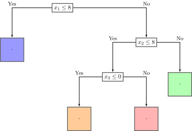
(a) Decision tree $T$ with four classes and no labels.

(b) Deterministic decision rule.

(c) Randomized decision rule.

Figure 2: Example of a tree $T$ (Figure 2(a)), a deterministic tree policy in $\Pi_{T}$ (Figure 2(b)) and a randomized tree policy in $\Pi_{T}$ (Figure 2(c)).

Our goal is to compute an optimal tree policy, i.e., our goal is to solve the Optimal Tree Policy (OTP) problem:

$$\min_{T\in\mathbb{T}}\min_{\pi\in\Pi_{T}}\;C(\pi)$$ (OTP)

Relations with classification trees. With a horizon of $H=1$, a tree policy is simply a decision rule that maps each state $s\in\mathbb{S}_{1}$ to a class $c\in[K]$ using a decision tree, then maps each class to an action $a\in\mathbb{A}_{1}$. If we identify the set of states $\mathbb{S}_{1}$ with the set of observations and the set of actions $\mathbb{A}_{1}$ with the set of labels, we see that instances of (OTP) (with $H=1$) and instances of (CT) are equivalent. The costs for the MDP instance play the role of the weights in the definition of the classification error (3.1) in the classification tree instance. We provide a formal proof of Proposition 3.3 in Appendix B.

Proposition 3.3.

Any instance of (OTP) with $H=1$ can be reduced to an instance of (CT). Additionally, any instance of (CT) can be reduced to an instance of (OTP) with $H=1$.

Since (CT) is an NP-hard problem (Laurent and Rivest 1976), Proposition 3.3 shows that solving (OTP) is an NP-hard problem. From our proof of Proposition 3.3, we also note that with a horizon $H=1$ and for a fixed tree $T_{1}$, computing an optimal policy in $\Pi_{T_{1}}$ is easy and can be done in a greedy fashion. When $\omega_{i,\ell}=1_{\{\ell=y_{i}\}}$ for $\ell\in\mathcal{L},i\in[m]$, this is analogous to the majority rule, where the label assigned to each class is simply the most represented label in each class. However, computing an optimal tree (along with the optimal policy) is NP-hard, even with $H=1$. This shows that when $H=1$, the hardness of (OTP) comes from computing an optimal decision tree: computing an optimal policy afterward is straightforward. Interestingly, Ciocan and Mišić (2020) consider the problem of computing tree policies for stopping time problems, and show that when $H\geq 2$ and a tree $T$ is fixed, computing an optimal policy in $\Pi_{T}$ is also NP-hard.

A first approach to computing tree policies. As highlighted in Proposition 3.3, it is hard to compute an optimal tree policy, even when $H=1$. Still, a natural heuristic to return tree policies can be as follows. First, compute the optimal unconstrained policy $\pi^{*}=\left(\pi^{*}_{1},...,\pi^{*}_{H}\right)$ for the MDP. This can be done efficiently with value iteration. Second, fit a classification tree to each of the optimal unconstrained decision rules $\pi_{1}^{*},...,\pi^{*}_{H}$.

Intuitively, this heuristic first solves the (unconstrained) MDP, then “projects” the optimal policy onto the set of tree policies. The problem with this approach is that for any $t\in\{1,...,H-1\}$, $\pi^{*}_{t}$ is the optimal choice of decision for period $t$ only if the decision maker chooses $\pi_{t+1}^{*},...,\pi^{*}_{H}$ subsequently. This follows from the recursion in the Bellman optimality equation (2.2). In particular, if the decision-maker modifies his/her decisions $\pi_{t+1}^{*},...,\pi^{*}_{H}$ to obtain tree policies, then $\pi^{*}_{t}$ may not be optimal at period $t$, and it is irrelevant to fit a tree to $\pi^{*}_{t}$. We characterize the optimal tree policies in the next section.

3.3 Structural Properties of optimal tree policies

In the unconstrained MDP setting presented in Section 2, an optimal policy may be chosen to be Markovian, deterministic, and independent of the initial distribution $\bm{p}_{1}$ (Puterman 1994). In the following proposition, we contrast these properties with the properties of optimal tree policies.

Proposition 3.4.

Consider an MDP instance $\mathcal{M}$, a set of sequence of trees $\mathbb{T}$ feasible for $\mathcal{M}$ and a feasible sequence of trees $T\in\mathbb{T}$.

1. All optimal tree policies for $T$ may depend on the initial distribution $\bm{p}_{1}$.

2. All optimal tree policies for $T$ may be history-dependent.

3. There always exists an optimal tree policy for $T$ that is deterministic (even though it may be history-dependent).

We present a detailed proof in Appendix C. Intuitively, in an instance of (OTP), the optimal decision at period $t$ depends on the current distribution over the states $\mathbb{S}_{t}$, which itself depends on the history up to period $t$. We also note that the optimality of deterministic policies is important for deploying policies in practice.

The role of rectangularity. We finish this section by discussing the fundamental role of rectangularity in value iteration and contrasting it with the decision tree structure. The rectangularity assumption is a common assumption in the robust optimization and robust MDP literature (Iyengar 2005, Bertsimas et al. 2011, Wiesemann et al. 2013, Goyal and Grand-Clément 2018). In the unconstrained MDP setting of Section 2.3, the rectangularity assumption states that the decisions $\pi_{t,s}$ for $s\in\mathbb{S}_{t}$ can be chosen independently across $s\in\mathbb{S}_{t}$. In particular, the decisions chosen in one state $s$ do not influence the choice of the decision maker at another state $s^{\prime}$ (at the same period). In this case, the minimization problems defining the recursions (2.2) on the value function $\bm{v}^{*}$ of the optimal policy $\pi^{*}$ can be solved independently across $s\in\mathbb{S}_{t}$ for every period $t\in[H]$. Crucially, this is also implies the component-wise inequality $\bm{v}^{*}_{t}\leq\bm{v}^{\pi}_{t}$ at any period $t$ for any Markovian policy $\pi$, since $\pi^{*}$ is solving the minimization programs (2.2) at each state independently. From the definition of tree policies (Definition 3.2), it is clear that the rectangularity assumption is not satisfied for tree policies, because if $\pi$ is a tree policy compatible with a given tree $T$, then $\pi$ must choose the same action for all the states in a given subregion of the state space (defined by a leaf of $T$). In this case, the recursion (2.2) may not hold for an optimal, interpretable policy. In particular, if there are some constraints across the decisions chosen at different states, a policy attaining the $\arg\min$ in (2.2) may not even be feasible.

3.4 Our algorithm

Since it is impractical to return history-dependent policies, we present an algorithm to compute Markovian tree policies. Our recursive algorithm, Algorithm 1, is based on the dynamic programming recursion (2.2), but it forces the sequence of decision rules $\pi_{1},...,\pi_{H}$ to be compatible with some trees $T_{1},...,T_{H}$. Our algorithm alternates between computing a decision rule $\pi_{t}$ for period $t$, compatible with a classification tree $T_{t}$, and updating the value function $\bm{v}_{t}$ of values obtained by the decision maker between period $t$ and $H$ when the decision rules are $\pi_{t},...,\pi_{H}$. It then proceeds backward to obtain the next decision rule $\pi_{t-1}$. Therefore, we interweave an algorithm for computing classification trees (e.g., CART) and an algorithm for computing optimal unconstrained policies (value iteration). This is in contrast with the more naive approach described after Proposition 3.3, that only uses CART after an optimal unconstrained policy $\pi^{*}$ has been computed.

Algorithm 1 Dynamic programming algorithm to compute a deterministic tree policy.

1:Input Sets of acceptable decision trees $\mathcal{T}(\mathbb{S}_{1},[K_{1}],\mathbb{A}_{1}),...,\mathcal{T}(\mathbb{S}_{H},[K_{H}],\mathbb{A}_{H})$ at periods $t=1,...,H.$

2:Initialize the policy. Let $t=H$ and $\hat{T}_{H}\in\mathcal{T}(\mathbb{S}_{H},[K_{H}],\mathbb{A}_{H}),\hat{\pi}_{H}\in\Pi_{H},$ solving

$$\min_{T\in\mathcal{T}(\mathbb{S}_{H},[K_{H}],\mathbb{A}_{H})}\min_{\pi\in\Pi_{T}}\sum_{c\in[K_{H}]}\sum_{s\in\mathbb{S}_{H}}\sum_{a\in\mathbb{A}_{H}}1_{\{T(s)=c\}}\pi_{sa}c_{H,sa}.$$

3:Initialize the value function. Set $\bm{v}_{H}\in\mathbb{R}^{\mathbb{S}_{H}}$ such that $v_{H,s}=\sum_{a\in\mathbb{A}_{H}}\hat{\pi}_{H,sa}c_{H,sa},\forall\;s\in\mathbb{S}_{H}.$

4:for $t=H-1,...,1$ do

5:     Choose the decision rule at period $t$. Compute $\hat{T}_{t},\hat{\pi}_{t}$ the optimal solutions to the following Optimal Tree Policy problem with horizon $H=1$:

$$\min_{T\in\mathcal{T}(\mathbb{S}_{t},[K_{t}],\mathbb{A}_{t})}\min_{\pi\in\Pi_{T}}\sum_{c\in[K_{t}]}\sum_{s\in\mathbb{S}_{t}}\sum_{a\in\mathbb{A}_{t}}1_{\{T(s)=c\}}\pi_{sa}\left(c_{sa}+\sum_{s^{\prime}\in\mathbb{S}_{t+1}}P_{sas^{\prime}}v_{t+1,s^{\prime}}\right).$$ (3.2)

6:     Update the value function. Set $\bm{v}_{t}\in\mathbb{R}^{\mathbb{S}_{t}}$ as

$$v_{t,s}=\sum_{a\in\mathbb{A}_{t}}\hat{\pi}_{t,sa}\left(c_{sa}+\sum_{s^{\prime}\in\mathbb{S}_{t+1}}P_{sas^{\prime}}v_{t+1,s}\right),\forall\;s\in\mathbb{S}_{t}.$$

7:end for

Discussion on Algorithm 1.

Several remarks are in order.

First, our algorithm alternates between computing decision rules that are compatible with a tree in Step 5, and updating the value function accordingly in Step 6. Given the value function $\bm{v}_{t+1}$, (3.2) is equivalent to an Optimal Tree Policy instance with $H=1$. From the equivalence of (OTP) and (CT) (Proposition 3.3), (3.2) can be solved with either exact methods (Bertsimas and Dunn 2017) or heuristics (Breiman et al. 1984).

Second, the optimal tree policy at period $t$ may depend of the distribution of the visited states $\mathbb{S}_{t}$, as follows from Proposition 3.4. This distribution depends on the previous decisions, i.e., it depends on $\hat{\pi}_{1},...,\hat{\pi}_{t-1}$. When we choose the decision rule $\hat{\pi}_{t}$ of period $t$ in Algorithm 1, we have chosen $\hat{\pi}_{t+1},...,\hat{\pi}_{H}$, but not yet $\hat{\pi}_{1},...,\hat{\pi}_{t-1}$. For this reason, we simply consider a uniform distribution over $\mathbb{S}_{t}$. In particular, in Step 5 we sum the continuation values associated with each state in $\mathbb{S}_{t}$. We then update the value function with the Bellman recursion in Step 6.

Finally, we would like to note that Algorithm 1 can be seen as a heuristic to return a good tree policy, by incorporating the changes in future decision rules in our current decision. This is in contrast to the naive approach presented after Proposition 3.3 (simply fitting a tree to the optimal unconstrained policy $\pi^{*}$), which does not take into account that modifying the actions chosen at period $t^{\prime}$ has an impact on the optimal actions in previous periods $t<t^{\prime}$. Because the optimal policy may be history-dependent, it appears hard to prove guarantees on the performances of the policies returned by Algorithm 1 or the naive approach. We will see in our numerical study that Algorithm 1 computes tree policies that can outperform state-of-the-art allocation guidelines, in the case of ventilator triage for COVID-19 patients.

4 Mechanical Ventilator Triage for COVID-19 Patients

In this section, we apply the methodology developed in Section 3 to develop interpretable triage guidelines for allocating ventilators to COVID-19 patients and compare them to existing triage guidelines.

4.1 Current triage guidelines

New York State (NYS) policy follows the 2015 Ventilator Triage Guidelines which were recommended by the NYS Taskforce on Life and the Law (Zucker et al. 2015). These guidelines were designed to ration critical care services and staff following a disaster (e.g., a Nor’easter, a hurricane, or an influenza epidemic). In particular, the guidelines outline clinical criteria for triage of patients using the Sequential Organ Failure Assessment (SOFA) score, a severity score that has been shown to correlate highly with mortality in COVID-19 (Zhou et al. 2020).

The goal of the NYS guidelines is to maximize the number of life saved. There are three decision epochs: at triage, the first time that a patient requires a ventilator; and thereafter, at two reassessment periods after 48 and 120 hours of intubation. The NYS triage guidelines defines priority classes – low, medium, and high – based on the current SOFA score of the patient. At the reassessment periods, the classification also depends on the improvement/deterioration of the SOFA score since the last decision epoch. A patient with low priority class will either be excluded from ventilator treatment (at triage) or removed from the ventilator (at reassessment). These patients typically either can be safely extubated, or have low survival chance (e.g., SOFA score $>$ 11). Patients with medium priority class are intubated and maintained on a ventilator, unless a patient with high priority class also requires intubation, in which case they are extubated and provided with palliative care. The guidelines at triage and reassessments admit simple tree representations (even though they were originally presented with tables). Details about the NYS guidelines are provided in Appendix D. We note that the NYS guidelines were defined in 2015 and, hence, are not specifically calibrated to the disease dynamics of COVID-19 patients.

4.2 Markov Model for COVID-19 Ventilator Triage

We now formalize the MDP model for COVID-19 ventilator allocation.

Decision epochs, states and epochs. Recall that the NYS guidelines has only three decision periods: at triage and two reassessments. Therefore, we consider an MDP model where there are $H=4$ periods; the last period corresponds to discharge of the patients after 120h (or more) of intubation. Our MDP model is depicted in Figure 3. After 0h/48h/120h of intubation, the patient is in a given health condition captured by the SOFA score (value of SOFA, and increasing/decreasing value of SOFA compared to last decision time), which changes dynamically over time, as well as static information on comorbidities and demographics.

At triage (0h of intubation, t=1 in the MDP), the decision maker chooses to allocate the ventilator to this patient, or exclude the patient from ventilator treatment. After 48h or 120h of intubation (t=2 and t=3 in the MDP), the decision is whether or not to maintain the patient on the ventilator. After the decision is executed, the patient transitions to another health condition or is nominally extubated before the next period which will correspond to a terminal state $D_{t}$ or $A_{t}$, indicating the status at discharge from the hospital (Deceased or Alive) (see Figure 3(a)). If the patient is excluded from ventilator treatment, s/he transitions to state $D_{t}^{ex}$ (if s/he dies at discharge) or $A_{t}^{ex}$ (if s/he recovers at discharge), see Figure 3(b).

Costs parameters. The MDP costs reflect the relative preference for survival of the patient (compared to death), with a penalty for longer use of ventilators in order to reflect the reluctance for lengthy use of limited, critical care resources. In particular, the costs are associated with terminal states $D_{t},A_{t},D_{t}^{ex},A_{t}^{ex}$, for $t\in\{1,2,3\}$ (modeling 0h/48/120h of intubation). Since we want to minimize the number of deaths, the costs of the deceased at discharge terminal states is significantly larger than that of the alive at discharge terminal states. Additionally, we want to penalize the lengthy use of resources, i.e., more costs should be given to discharge after 120h (or more) of intubation compared to discharge after 0h to 48h of intubation, in order to capture the disutility of using the limited ventilator capacity. Finally, for a given outcome (deceased or alive), we aim to distinguish among the states where the patient was excluded or not.

To capture these considerations, we parametrize our cost function with three parameters. We let $C>1$ represents the cost for deceased patients, which is measured relative to a base cost of $1$ for patients who survive. Typically, $C$ one or two orders of magnitude higher than $1$; in our simulation we choose $C=100$. To penalize for using the limited resource, the cost for ventilator use increases by a multiplicative factor $\rho>1$ for each period of ventilator use (corresponding to 48h, 120h, 120+h). This can be seen as an actualization factor, e.g., $\rho=1.1$ means that future costs are increasing by $10\%$ (per period) compared to the same outcome at the current period. This cost reflects the desire to use resources for shorter periods. We choose $\rho=1.1$ in our simulation. Finally, among patients who survive, a multiplicative penalty of $\gamma>1$ is given to patients who have been extubated, while for patients who die, a multiplicative bonus of $1/\gamma<1$ is given to patients who have been extubated. Choosing $\gamma$, one needs to be careful to maintain the costs for deceased patients higher than the costs for patients discharged alive. We choose $\gamma=1.5$ in our simulation. We recommend values of $C,\rho$ and $\gamma$ to maintain $C/\gamma>>\gamma\rho^{2}$, so that any state associated with deceased patients have higher costs than any state associated with patients alive at discharge. Our final costs functions can be represented as

$$c(A_{t}^{\sf\ell})=1\times\rho^{t-1}\times\gamma^{\mathbbm{1}_{\{\ell=\sf ex\}}},\;c(D_{t}^{\sf\ell})=C\times\rho^{t-1}\times(1/\gamma)^{\mathbbm{1}_{\{\ell=\sf ex\}}},\forall\;t\in\{1,2,3\}.$$

While this cost parametrization is an artifact of our model and is necessary to compute the triage policy, we evaluate the performance of the resulting policy through simulations, which estimate its potential performance in practice. We also conduct a sensitivity analysis, where we vary the values of $C,\rho$ and $\gamma$, and study the variations in the estimated performances of the corresponding optimal policies and tree policies in the MDP. We observe stable performances in the simulation model for the optimal policies and tree policies for a wide range of parameters $C,\rho,\gamma$, as long as $C/\gamma$ is significantly larger than $\gamma\rho^{2}$. We present the sensitivity analysis in Appendix G,

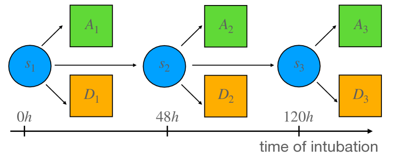
(a) Transition for action = maintain.

(b) Transition for action = exclude.

Figure 3: States and transitions in our MDP model with actions ‘maintain’ and ‘exclude’.

4.3 Data set and parameter estimation

To calibrate our model, we utilize a retrospective data of 807 COVID-19 hospitalizations at Montefiore. In particular, we include patients with confirmed laboratory test (real-time reverse polymerase chain reaction) for SARS-CoV-2 infection, admitted to three acute care hospitals within a single urban academic medical center from 3/01/2020 and 5/27/2020, with respiratory failure requiring mechanical ventilation. This hospital system is located in the Bronx, NY, which was one of the hardest hit neighborhoods during the initial COVID-19 surge seen in the United States. This study was approved by the Albert Einstein College of Medicine/Montefiore Medical Center and Columbia University IRBs.

Each hospitalization corresponds to a unique patient. For each patient, we have patient level admission data. This includes demographics such as age, gender, weight, BMI, as well as comorbid health conditions such as the Charlson score, diabetes, malignancy, renal disease, dementia, and congestive heart failure. Our data provides admission and discharge time and date, as well as status at discharge from the hospital (deceased or alive). Finally, every patient in our data set is assigned a SOFA score, which quantifies the number and severity of failure of different organ systems  (Jones et al. 2009), and which is updated every two hours. The ventilator status of the patients (intubated or not) is also updated on a two-hours basis.

The hospital that we study was able to increase ventilator capacity through a series of actions, including procurement of new machines, repurposing ventilators not intended for extended use, and borrowing of machines from other states. The maximum number of ventilators that were used for COVID-19 patients over the study period was 253. The hospital never hit their ventilator capacity, so triage was never required to determine which patients to intubate.

The mean SOFA score at admission was 2.0 (IQR: [0.0,3.0]) and the maximum SOFA score over the entire hospital stay was 9.7 (IQR: [8.0,12.0]). The mean age was 64.0 years (SD 13.5). The patients who survived were significantly younger than those who died in the hospital (p$<$0.001). The average SOFA at time of intubation was 3.7 (IQR: [1.0,6.0]), at 48 hours it was 6.3 (IQR: [4.0,9.0]) and at 120 hours it was 5.9 (CI: [3.0,8.0]). Details and summary statistics about the data set and our patient cohort are presented in Table 1 in Appendix H.

4.4 Model Calibration

To calibrate the MDP model, we utilize static patient data assigned at the time of admission (e.g., history of comorbodities), and dynamical patient data updated on a two-hour basis (e.g., SOFA score and intubation status). We calibrate the transition rates across states, as well as the likelihood of deaths and survival at each period, using the observed rates for these events from the data. The transition rates depend on the information included in the states. To reduce the total number of states and to increase the number of observations and transitions per states, we first create $k=10$ clusters using $k$-means when using more information than just the SOFA score. A state then consists of a cluster label, and the current SOFA score, and the direction of change of the SOFA score (decreasing or increasing, compared to last triage/reassessment period).

Note that in our data we do not observe any early extubation (i.e., we only observe extubation when it is safe or when the patient is deceased). Therefore, we cannot estimate the transition rates to $D^{ex}_{t}$ (the death state if extubated between period $t$ and the next period). We use a single parameter $p\in[0,1]$ for the transitions to $D^{ex}_{t}$. We choose a uniform $p$ across periods $t\in\{1,2,3\}$ and states. This gives a range of estimates, from optimistic estimates ($p=0$) to more realistic estimates ($p\geq 0.9$), with values $p=0.90$ and $p=0.95$ being closer to the death rates estimated by our clinical collaborators.

We note that some patients may be intubated more than once during their hospital visits. This can happen when the health condition of an intubated patient first improves, the patient is safely extubated, and then the health condition starts to deteriorate again. We do not account for this in our MDP model, as this is a relatively rare event. In our data, it occurs in only 5.7% of the patients. Therefore, we treat second ventilator uses as new trajectories, starting from period $t=1$. While the dynamical health evolution of the patient who are reintubated may differ from the dynamics of the patients who are intubated for the first time, we emphasize that only the computational part (i.e., computation of tree policies for the MDP in Figure 3) is based on this approximation. The evaluation of patient survival with our simulation model does not depend on this approximation.

4.5 Policy Computation

We use Algorithm 1 for our MDP model to compute several tree policies using different covariates describing the health conditions of the patients. We first compute a tree policy that only uses the SOFA score (Figure 12), since this is the only covariate used in the NYS guidelines. We then compute a tree policy based on SOFA and age of the patient (Figure 13), as there is some debate about making categorical exclusions based on age: for example, the NYS guidelines break ties based on age. We also compute a tree policy based on all the comorbid conditions and demographic information available in our data (Figure 14). When we include covariates other than SOFA scores, we create 10 clusters to reduce the final number of states and transitions. For instance, for the policies based on SOFA scores and age, the final states in the MDP of Figure 3 consists of pairs $({\sf sofa},\ell,+/-)$ where ${\sf sofa}$ is the current SOFA score, $\ell$ is a cluster label describing the age of the patient, and $+$ or $-$ captures whether patient condition is improving or worsening. We present the details of the covariates used in the full tree policy along with the corresponding trees for each computed policy in Appendix E .

We note that one needs to be cognizant of potential ethical considerations when including certain covariates. For instance, diabetes has been shown to be correlated with higher risk of severe COVID (Orioli et al. 2020). However, increased prevalence of diabetes (and other risk factors for severe COVID patients) is observed in underserved communities who have suffered from structural health inequities. Excluding patients from ventilator access on the basis of such covariate could further exacerbate these long-standing structural inequities. As such, there are several ethical justifications for the absence of categorical exclusion criteria from the triage decisions (White and Lo 2020). During the COVID-19 pandemic, there has been a movement away from including these covariates in triage algorithms, because of the potential to exacerbate inequities (Mello et al. 2020). We believe there is value in estimating the potential benefits (or not) of including as much information as possible in the triage guidelines, to provide quantitative data on the consequences of these choices to inform this discourse.

5 Empirical results

We evaluate the performance of the tree policies computed using Algorithm 1. We compare to two benchmarks: 1) NYS Triage guidelines and 2) First-Come-First-Serve (FCFS). For all policies – including ours – ventilators are allocated according to FCFS until the ventilator capacity is reached. When there is insufficient ventilator supply to meet all of the demand, they will be allocated according to the specified priority scheme.

5.1 Simulation model

We use simulation to estimate the number of deaths associated with implementation of the various triage guidelines at different levels of ventilator capacity. Specifically, we bootstrap patient arrivals and ventilator demand from our data and examine different allocation decisions, based on our MDP model. The time periods considered consist of a discretization of the time interval (03/01/20 - 05/27/20) into intervals of two hours. At each time period, the following events happen:

1. We sample (with replacement) the arrivals and ventilator demand from our data set of observed patients trajectories. The number of samples at each period is equal to the number of new intubations observed at this time period in our data.

2. We update the status (intubated, reassessment or discharge) of all patients in the simulation. Prior to reaching ventilator capacity, ventilators are allocated on a first-come-first served basis. When the ventilator capacity is reached, new patients are triaged using the triage guideline chosen and assigned a priority (low, medium or high). Low priority patients are excluded from ventilator treatments. A medium priority patient currently intubated may be excluded from ventilator treatment, to intubate a high priority patient. High priority patients are never extubated. In particular, if all patients currently intubated have high priority, any remaining patients who need a ventilator will be excluded from ventilation; i.e., no patients currently intubated will be excluded from ventilator treatment.

3. After 48h and 120h of intubation, patients on ventilators are reassessed and reassigned priority classes. Patients in low and medium priority classes are excluded from ventilator treatment if a new patient with higher priority requires one. Patients with low priority class are removed first.

The First-Come-First-Served (FCFS) triage rule is operationalized as follows. When the capacity constraint is reached, no new patient is assigned a ventilator until one becomes available, regardless of priority classes. Extubation only occurs when the patient is deceased or can be safely extubated (the timing of which is indicated by extubation in the observed data).

At discharge, the status of patients who were not impacted by the triage/reassessment guidelines (i.e. their simulated duration of ventilation corresponds to the observed duration in the data) is the same as observed in the data. For the outcomes of patients excluded from ventilation by the triage guideline, we use the same method as for our MDP model. In particular, we use a single parameter $p\in[0,1]$ to model the chance of mortality of patients excluded from ventilator treatment. With probability $p$, the discharge status of a patient excluded from ventilator treatment is deceased. Otherwise, with probability $1-p,$ the discharge status of a patient excluded from ventilator treatment is the same as if this patient had obtained a ventilator (i.e., the same as observed in the data). We acknowledge that the three potential exclusion events (at triage, at reassessments, or when removed in order to intubate another patient) may require different values of $p$. Additionally, $p$ may vary across patients and is difficult to estimate in practice. However, when $p=0$, we obtain an optimistic estimate of the survival rate, since being excluded from ventilator treatment has no impact on the outcome of the patient. When $p=1$, we obtain a pessimistic estimate of the survival rate, as in this case any patient excluded from ventilator treatment will die. Therefore, using a single parameter $p$ in $[0,1]$ enables us to interpolate between an optimistic ($p=0$) and a pessimistic ($p=1$) estimation of the survival rates associated with the triage guidelines. In practice, our clinical collaborators estimate that $p=0.90$ or $p=0.95$ are reasonable values.

5.2 Number of deaths

We obtain estimate of the number of deaths, associated with a ventilator capacity and triage guidelines over $100$ bootstrapped data sets. In Figure 4, we compare the number of deaths associated with various levels of ventilator capacity for different triage guidelines: our tree policies based only on SOFA, based on SOFA and age, and based on SOFA and other covariates. For comparison purposes, we also include the performance of the NYS triage algorithm and FCFS. We also show the performance of the optimal unconstrained policy for our MDP model (which we call MDP policy in Figure 4). For the sake of readability, we only show the MDP policy computed based on SOFA score, as it is outperforming the MDP policies based on SOFA score and age, and SOFA score and other covariates. Recall that $p$ models the likelihood of death of a patient after exclusion from ventilator treatment. For brevity, we only present the pessimistic ($p=0.99$) estimations in the main body of the paper. The estimations for other values of $p$ are coherent with $p=0.99$ and are presented in Appendix F. We recall that the total number of deaths in our data set, i.e., with ample ventilator capacity, was 543 patients among our cohort of 807 patients (see Table 1).

We see similar number of deaths between the NYS and FCFS policies. For instance, we consider the number of deaths at a ventilator capacity of 180 ventilators. The average total for the number of deaths is 582.9 (CI: [582.3,583.4]) for the NYS guidelines and 585.3 (CI: [584.5,586.1]) for the FCFS guidelines. While the difference in the number of deaths is statistically significant (at the p$<$0.001 level), this difference is small (two to three lives, less than 0.5% of the total 543 observed deaths over a time period when triage was never necessary). In Figure 4 we observe this very small difference between the two policies for various levels of ventilator capacity. This also holds for various levels of $p\in[0,1]$ (see Appendix F). It is somewhat surprising to see the NYS and FCFS guidelines performing similarly in this cohort of COVID-19 acute respiratory failure. The NYS guidelines were designed prior to the COVID-19 pandemic, in part because of concerns that arose following the shortages experienced in New Orleans after Hurricane Katrina. Consequently, they were designed primarily for the case of ventilator shortages caused by disasters, such as hurricanes, a Nor’easter, or mass casualty event. Therefore, even though the NYS guidelines is based on the SOFA score, it ignores the specifics of respiratory distress caused by COVID-19. For instance, this may indicate that COVID-19 natural history does not follow the 48 and 120 hours reassessment time line, with the average SOFA score at t=48h and at t=120h being somewhat similar in our patient cohort. The timing of reassessment in the NYS guidelines may need to be re-examined, otherwise the NYS triage algorithm is not able to substantially outperform FCFS.

Figure 4: Number of deaths for various triage guidelines at hypothetical levels of ventilator capacities, for $p=0.99$.

Still focusing on a ventilator capacity of 180 ventilators, we note that when only using information on SOFA, our tree policy achieves an average number of deaths of 574.1 (CI: [573.4,574.7]). The difference with the average number of deaths for the NYS guidelines amounts to 1.5 % of the 543 observed deaths in our data. The optimal MDP policy only based on SOFA performs even better (average: 568.5 deaths, CI: [567.8,569.1]) but is not interpretable. We present our tree policy in Appendix E. It is a very simple policy, which only excludes patients with SOFA strictly higher or equal to $11$ at triage and strictly higher or equal to 10 at reassessment. Thus, it is less aggressive than the NYS guidelines which may exclude some patients with SOFA $>7$ at 48h and 120h of intubation, if their conditions is not improving (see Appendix D for more details). This suggests that the NYS guidelines may be too proactive at excluding patients from ventilator treatments.

We note that including other covariates (such as demographics and comorbidities, see Tree policy (SOFA+COV) in Figure 4) leads to similar performances compared to policies only based on SOFA score. This is coherent with the fact that the SOFA score itself has been shown to be a strong predictor of COVID-19 mortality (Zhou et al. 2020). When we only include SOFA and age (Tree policy (SOFA+AGE) in Figure 4), we see higher number of deaths for the estimated tree policy, compared to policies only based on SOFA score. We note that including more covariates in the state space leads to a smaller number of transitions out of each state, leading to less accurate parameter estimations (even though we use clusters to lower the number of states in our MDP model). Therefore, this may reflect the fact that age is not a good predictor for COVID-19 mortality, so that including it in the state space only results in lower accuracy for parameter estimations, and does not result in a more informative description of the health state of the patient. Overall, the models that incorporate comorbidities and/or demographics do not significantly outperform the policies only based on SOFA. Categorical exclusion of some patients is considered unethical (White and Lo 2020), and we show that it is not necessarily associated with significant gains in terms of patients saved.

5.3 Observed survival rates among excluded patients

For each level of ventilator capacity and each triage guideline (NYS, FCFS, or tree policies), using our simulation model we can compute the list of patients that would have been excluded from ventilator treatments. In an ideal situation, triage guidelines would exclude from ventilator treatment patients who would not benefit from it, i.e., ideal triage guidelines would exclude the patients that would die even if intubated. Note that using our data set we are able to know if a patient would have survived in case of intubation (since all patients were intubated in our data set and we can see status at discharge). Therefore, we can compute the survival rates (in case of intubation) among excluded patients. Intuitively, if the guidelines were perfect, the survival rate (in case of intubation) among excluded patients would be close to 0 %. Note that random exclusion would achieve an average survival rate (in case of intubation) among excluded patients of 32.7 %, the average survival rate in our cohort of patients.

We compare the survival rate (in case of intubation) among excluded patients for various guidelines in Figure 5-8. In Figure 5(b), we note that among the patients excluded by the NYS guidelines at triage, the survival rate in case of intubation would have been above 40 % (for all levels of ventilator capacity). This is higher than 32.7 % (p$<$0.001), which means that at triage, the NYS guidelines are mis-identifying patients who would not benefit from ventilator treatment. At reassessment, and compared to triage, the NYS guidelines achieve lower survival rates (in case of intubation) among patients excluded (Figure 5(c)). Compared to NYS guidelines, our novel triage guidelines based on SOFA, SOFA and age, and SOFA, demographics and comorbidities, are identifying for exclusion those patients with lower survival rates (when intubated) (Figures 6(a), 7(a),8(a)). We note that the tree policy based on SOFA, demographics and comorbidities does not exclude any patient at triage (Figure 8(b)). Additionally, among all policies, the survival rates (in case of intubation) among patients excluded at triage is higher than the observed survival rates among patients excluded at reassessment. This stark discrepancy between performances at triage and at reassessment suggests that it is significantly harder to foreshadow the future evolution of patients condition and status at discharge, at the moment of intubation. All the guidelines considered better identify patients who would not benefit from ventilator treatment, after the patients have been intubated for at least 48h. This may suggest that there should be more proactive decisions about withdrawing support from the patients who are not responding to intensive care treatment. Although ethicists generally consider the decision to proactively extubate a patient at reassessment morally equivalent to declining to offer intubation at triage, this action may cause more moral distress to clinicians carrying out the extubation (see Chapter 5 in (Beauchamp et al. 2001)).

Finally, we want to note that it is also important to account for the number of patients excluded by the guidelines. In particular, Figure 7(a) (for the tree policy based on SOFA and age) is very similar to Figure 6(a) (for the tree policy only based on SOFA) and Figure 8(a) (for the tree policy based on SOFA and other covariates). In contrast, we have seen in Figure 4 that the tree policy based on SOFA and age may perform quite poorly. Using our simulation model, we noted that on average it was excluding more patients. For instance, at a ventilator capacity of 180, it is excluding on average 233.5 patients (CI: [221.4,245.6]) compared to 191.7 patients for the tree policy based on SOFA (CI: [176.6, 206.8]) and 189.4 patients for the tree policy based on SOFA and other covariates (CI: [176.3,202.5]). This is mainly the reason behind the poor performance of the tree policy based on SOFA and age: even though it maintains a similar survival rate (in case of intubation) among excluded patients, it exclude more patients than the other tree policies, some of which would have survived in case of intubation. The other tree policies are striking a better balance between excluding many patients and identifying patients who would not benefit from ventilator treatment.

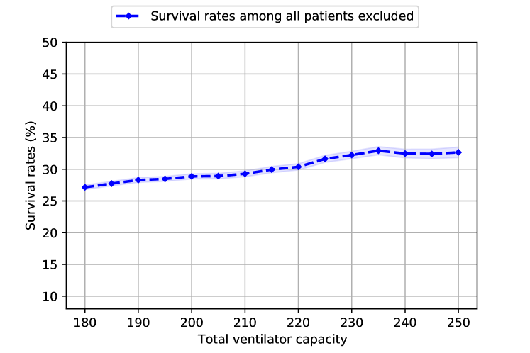
(a) All excluded patients.

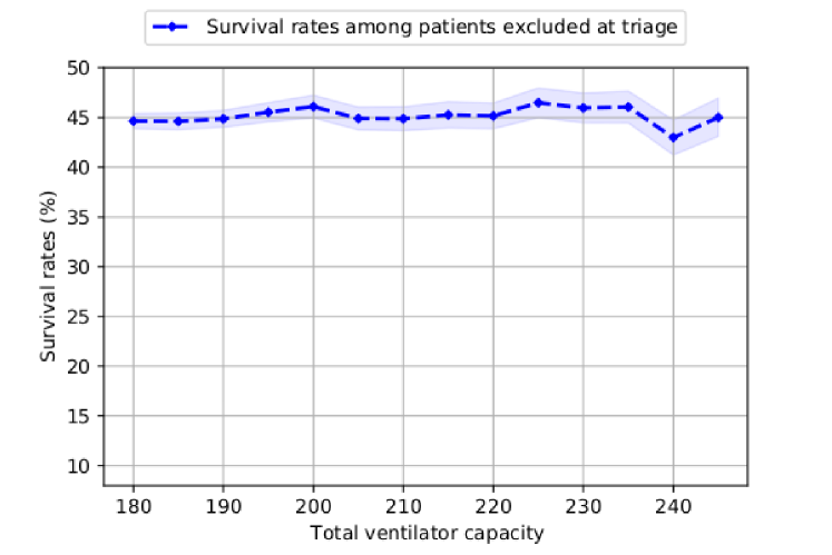
(b) Patients excluded at triage.

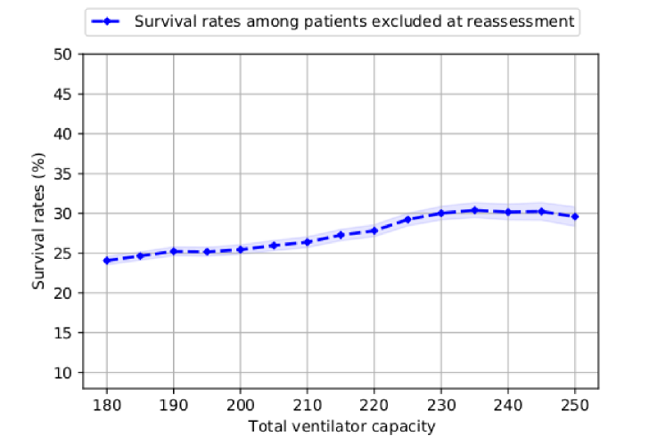
(c) Patients excluded at reassessment.

Figure 5: For NYS guidelines: observed survival rates (in the case of intubation) among all excluded patients (Figure 5(a)), patients excluded at triage (Figure 5(b)) and patients excluded at reassessment (Figure 5(c)).

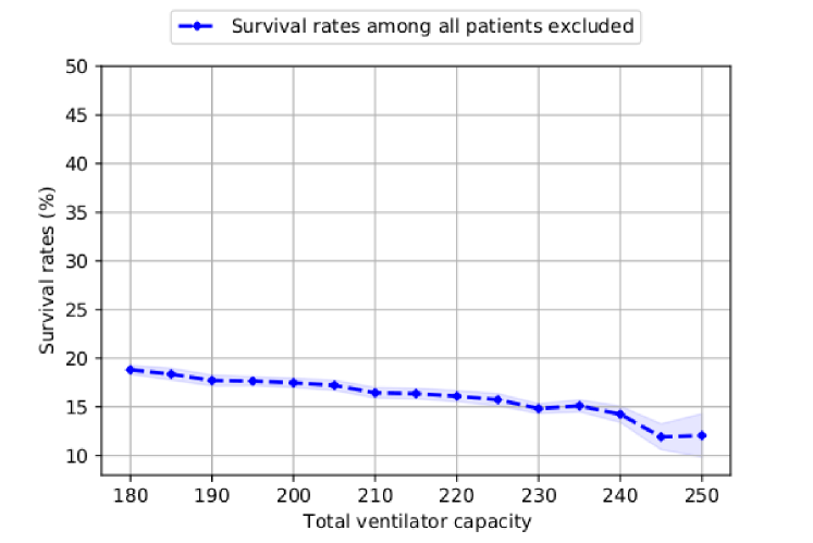
(a) Among all excluded patients.

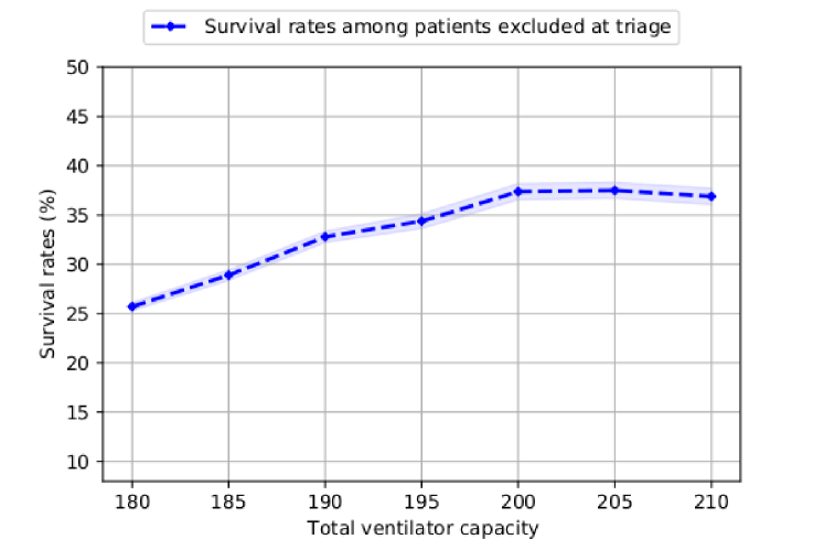
(b) Among patients excluded at triage.

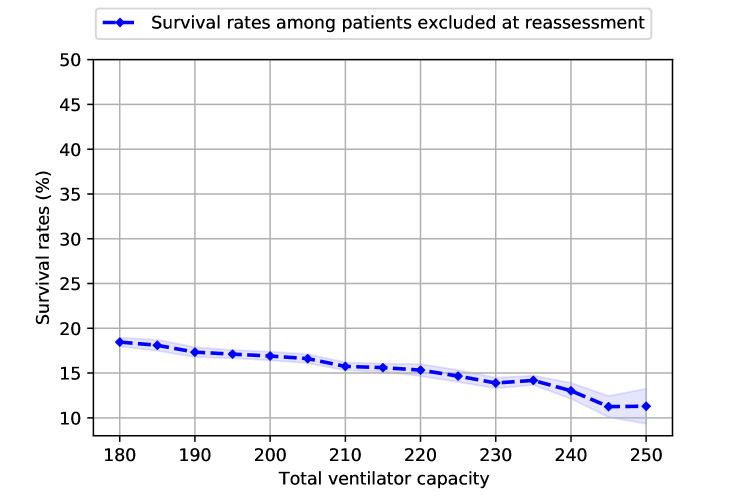
(c) Among patients excluded at reassessment.

Figure 6: For our tree policy only based on SOFA score: observed survival rates (in the case of intubation) among all excluded patients (Figure 6(a)), patients excluded at triage (Figure 6(b)) and patients excluded at reassessment (Figure 6(c)).

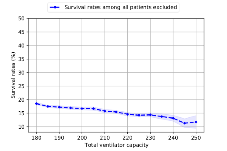
(a) Among all excluded patients.

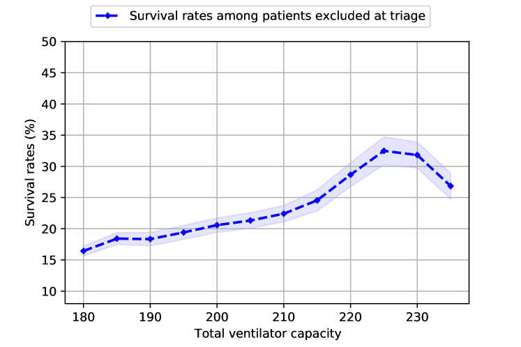
(b) Among patients excluded at triage.

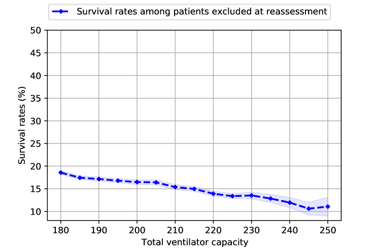
(c) Among patients excluded at reassessment.

Figure 7: For our tree policy only based on SOFA score and age: observed survival rates (in the case of intubation) among all excluded patients (Figure 7(a)), patients excluded at triage (Figure 7(b)) and patients excluded at reassessment (Figure 7(c)).

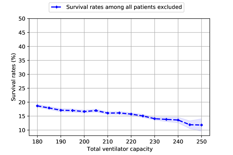
(a) Among all excluded patients.

(b) Among patients excluded at triage.

(c) Among patients excluded at reassessment.

Figure 8: For our tree policy based on SOFA score, demographics and comorbidities: observed survival rates (in the case of intubation) among all excluded patients (Figure 8(a)), patients excluded at triage (Figure 8(b)) and patients excluded at reassessment (Figure 8(c)).

5.4 Discussion

Advantages and disadvantages of SOFA-based guidelines. SOFA-based guidelines have multiple advantages. First, the SOFA score has been shown to correlate with COVID mortality (Zhou et al. 2020). They are simple to implement, as they rely on a single score, and can be deployed quickly in a number of different clinical and disaster scenarios before specifics of a new disease are known. This is why of the 26 states who have defined triage guidelines in the United States, 15 use the Sequential Organ Failure Assessment (SOFA) score to triage patients (Babar and Rinker 2016).

In terms of performance, we have seen in Figure 4 that SOFA policies may achieve lower number of deaths than the official NYS policies (here, COVID-19). This suggests that NYS guidelines, also solely relying on SOFA scores, need to be adjusted to the current disaster before being successfully implemented. It may be possible to improve the performance of triage policies when even more disease-specific data become available, however, this will not solve the problem of how to manage a novel disaster in the future.

Intuitively, incorporating more covariates in the decision model may help better inform triage guidelines. In contrast, our data show that using other clinical information (such as demographics and comorbidities) does not necessarily improve the number of lives saved. Additionally, including comorbid conditions may further disadvantage those who face structural inequities, since comorbidities such as diabetes and obesity are closely linked to social determinants of health (Cockerham et al. 2017). This detrimental impact may erode trust in medical institutions at large (Auriemma et al. 2020), which in turn may frustrate other critical public health interventions such as vaccination (Bunch 2021). Therefore, it is critical to counterbalance the utilitarian aims of saving more lives with fairness and the duty to patient care. Designing data-driven and explainable guidelines is a first step toward fair and efficient allocation of resources. This study provides some data to inform the process of choosing to implement (or not) triage guidelines: official guidelines (such as NYS guidelines) need to be re-adjusted to the specifics of COVID-19 patients before being implemented. Otherwise, they may show little to no improvement compared to FCFS guidelines, and there may not be any ethical justification for unilaterally removing a patient from a ventilator and violating the duty to care for that patient.

Limitations. The strength of our analysis is based on real world data during a massive surge in our facility where ventilator capacity reached fullness. There are several limitations to this study. First, the results cannot be applied to other disease states such as novel viruses that may arise in the future. The model needs to be re-trained with new data for each specific patient population. Second, the observations occurred during the height of the pandemic in New York City when little was known about the specific management of COVID-19. Results may be different with better therapeutic options for the disease. However, this is also a strength of the study given that it matches the scenarios in which triage guidelines are meant to be deployed. Third, the results could be different under different surge conditions, e.g. if the rise in number of cases was sharper or more prolonged. Finally, the simulation cannot mimic real-world work flows that might have required some alterations of the movement of ventilators between patients. From a modeling standpoint, our algorithm may not return an optimal tree policy, since it only returns Markovian tree policies. Additionally, we use a nominal MDP model, and do not attempt to compute a robust MDP policy (Iyengar 2005, Wiesemann et al. 2013, Goyal and Grand-Clément 2018). This reason behind this is that we have a fairly small population of patients, so that the confidence intervals in the estimation of our transition rates may be quite large, leading to overly conservative policies. To mitigate this, we use our simulation model to estimate the performances of a policy, and not simply the cumulative rewards in the MDP model, which, of course, also depends of our parameter choices. Therefore, even though the triage guidelines computed with Algorithm 1 are dependent of the (possibly miss-estimated) transition rates and our choices of costs, the estimation of their performances is not, and is entirely data- and expert-driven, relying solely on our data set of 807 patients hospitalizations and our collaborations with practitioners at Montefiore.

6 Conclusion

In this work we study the problem of computing interpretable resource allocation guidelines, focusing on triage of ventilator for COVID-19 patients. We present an algorithm that computes a tree policy for finite-horizon MDPs by interweaving algorithms for computing classification trees and algorithms solving MDPs. Developing bounds on the suboptimality of this tree policy compared to the optimal unconstrained policy is an important future direction. Additionally, we provide valuable insights on the performances of official triage guidelines for policy makers and practitioners. We found that the New York State (NYS) guidelines may fail to lower the number of deaths, and performs similarly as the simpler First-Come-First-Served allocation rule. Our empirical study finds that our interpretable tree policies based only on SOFA may improve upon the NYS guidelines, by being less aggressive in exclusions of the patients. Some medical studies have found that SOFA may not be informative for Sars-CoV-2 triage decisions (Wunsch et al. 2020). We show that SOFA is not necessarily useless, but this depends greatly on how the decision maker uses it. Remarkably, our simulations also show that it may not be beneficial to include more information (e.g., demographics and comorbidities) in the triage and reassessment recommendations. In particular, this may not lead to lower number of deaths, on the top of raising important ethical issues. Overall, our simulations of various triage guidelines for distributing ventilators during the COVID-19 pandemic revealed serious limitations in achieving the utilitarian goals these guidelines are designed to fulfill. Guidelines that were designed prior to the pandemic need to be reconsidered and modified accordingly to incorporate the novel data available. Our work can help revise guidelines to better balance competing moral aims (e.g., utilitarian objectives vs. fairness). Interesting directions include studying guidelines with later times of reassessments (e.g., reassessment after $7$ or $10$ days on ventilators) or different objectives (such the total number of life-years saved).

Appendix A Linear reformulation of the randomized classification error

In this appendix we show that our cost function can be reformulation as a linear objective using some binary and scalar variables. In particular, recall that our cost function for optimal classification tree problem is

$$C_{\sf tree}(T)=\sum_{c=1}^{K}\sum_{i=1}^{m}\sum_{\ell\in\mathcal{L}}\omega_{i,\ell}1_{\{T(\bm{x}_{i})=c\}}\mu_{c,\ell},$$

where $\bm{\mu}_{c}\in\Delta(\mathcal{L})$ is the distribution over labels $\ell\in\mathcal{L}$ chosen for the class $c\in[K]$. Note that this objective is the weighted sum of some products of binary variables ($1_{\{T(\bm{x}_{i})=c\}}\in\{0,1\}$) and continuous variables ($\mu_{c,\ell}\in[0,1]$). Classical reformulation tricks show that for all $(c,i,,\ell)\in[K]\times[m]\times\mathcal{L}$, each product $1_{\{T(\bm{x}_{i})=c\}}\mu_{c,\ell}$ can be linearized by introducing a third variable $z_{i,c,\ell}$, writing the objective as

$$C_{\sf tree}(T)=\sum_{c=1}^{K}\sum_{i=1}^{m}\sum_{\ell\in\mathcal{L}}\omega_{i,\ell}z_{i,c,\ell},$$

and introducing the following constraints to the MILP formulation of (CT):

$$z_{i,c,\ell} \leq 1_{\{T(\bm{x}_{i})=c\}},$$

$$z_{i,c,\ell} \leq\mu_{c,\ell},$$

$$\mu_{c,\ell}+1_{\{T(\bm{x}_{i}=c\}}-1 \leq z_{i,c,\ell},$$

$$0 \leq z_{i,c,\ell}.$$

Appendix B Equivalence of Optimal Tree Policies and Optimal Classification Trees

In this appendix we show the proof of our Proposition 3.3, which established the equivalence between (CT) and (OTP) when $H=1$.

Proof of Proposition 3.3..

1. Any instance of (OTP) with $H=1$ can be reduced to an instance of (CT). Let us consider an MDP instance $\mathcal{M}=(H,\mathbb{S}_{1},\mathbb{A}_{1},\bm{P}_{1},\bm{r}_{1},\bm{p}_{1})$ with horizon $H=1$. Let $T\in\mathbb{T}$ and $\pi\in\Pi_{T}$. In this case, note that $T=\left(T_{1}\right)$ where $T_{1}\in\mathcal{T}(\mathbb{S}_{1},[K_{1}],\mathbb{A}_{1})$. The cost $C(\pi)$ of $\pi$ is

   $$C(\pi)=\sum_{s\in\mathbb{S}_{1}}\sum_{a\in\mathbb{A}_{1}}p_{1s}\pi_{sa}r_{sa}=\sum_{c=1}^{K_{1}}\sum_{s\in\mathbb{S}_{1}}1_{\{T(s)=c\}}\left(\sum_{a\in\mathbb{A}_{1}}p_{1s}\pi_{sa}r_{sa}\right).$$

   Note that for any class $c\in[K_{1}]$, $a\mapsto\pi_{1,sa}$ is the same map for all $s\in T^{-1}_{1}(c)$. With a small abuse of notation, we write this map $a\mapsto\pi_{ca}$. Therefore, the cost $C(\pi)$ can be written

   $$C(\pi)=\sum_{c=1}^{K_{1}}\sum_{s\in\mathbb{S}_{1}}\sum_{a\in\mathbb{A}_{1}}\left(p_{1s}r_{sa}\right)1_{\{T(s)=c\}}\pi_{ca}.$$

   This is exactly the expression of the weighted classification error as in (3.1). Therefore, (OTP) with horizon $H=1$ reduces to (CT).

2. Any instance of (CT) can be reduced to an instance of (OTP) with $H=1$. Let $\mathcal{D}$ be an instance of CART. In particular, let $\mathcal{D}=\{(\bm{x}_{1},y_{1}),...,(\bm{x}_{m},y_{m})\}$ a sequence of $m$ pairs of points and labels, with $\bm{x}_{i}\in\mathbb{S}\subset\mathbb{R}^{p}$ and $y_{i}\in\mathcal{L}\subset\mathbb{N}$. We are also given some weights $\left(\omega_{i,\ell}\right)_{i,\ell}$ for the classification error and a set of admissible tree $\mathcal{T}\left(\mathbb{S},[K],\mathcal{L}\right)$. The goal is to find a decision tree in $\mathcal{T}\left(\mathbb{S},[K],\mathcal{L}\right)$ that minimizes the classification error $C_{\sf tree}(T)$ defined as in (3.1).

   We can reduce this instance of (CT) to an instance of (OTP). In particular, we define the MDP instance $\mathcal{M}=(H,\mathbb{S}_{1},\mathbb{A}_{1},\bm{P}_{1},\bm{r}_{1},\bm{p}_{1})$ as follows:

   1. The horizon is $H=1$.

   2. The set of states is the set of possible features: $\mathbb{S}_{1}=\{\bm{x}_{1},...,\bm{x}_{m}\}$.

   3. The set of actions is the set of labels: $\mathbb{A}_{1}=\{y\;|\;\exists\;i\in\{1,...,m\},y_{i}=y\}$.

   4. The choice of $\bm{P}_{1}$ (transition kernels) does not play any role, because $H=1$.

   5. The costs $\left(c_{1,sa}\right)_{s,a}$ are constructed to reflect the weights $\left(\omega_{i,\ell}\right)_{i,\ell}$. In particular, if $s\in\mathbb{S}_{1}$ and $a\in\mathbb{A}_{1}$, by construction $s=x_{i}$ and $a=\ell$ for some $i\in[m]$ and some possible label $\ell$. The cost $c_{sa}$ is chosen as $\omega_{i,\ell}$.

   6. The initial distribution is uniform across all states.

   With this formulation, for any admissible tree $T\in\mathcal{T}\left(\mathbb{S},[K],\mathcal{L}\right)$, a tree policy $\pi\in\Pi_{T}$ is equivalent to assigning a probability distribution over $\mathcal{L}$ to each point $\bm{x}_{i}$ for every $i\in[m]$, with the additional constraint that the same distribution is chosen for all observations belonging to the same class. The cost $C(\pi)$ associated with a policy is the classification cost $C_{\sf tree}(T)$ of the tree $T$. Therefore, solving the (OTP) problem with this MDP instance solves the (CT) problem with instance $\mathcal{D}$.

∎

Appendix C Properties of Optimal Tree Policies

In this appendix we show the proof of our Proposition 3.4, which established the main properties of optimal tree policies.

Proof of Proposition 3.4..

1. All optimal tree policies for $T$ may be dependent on the initial distribution $\bm{p}_{1}$ over the set of first states $\mathbb{S}_{1}$. We consider an example of Optimal Tree Policy instance where $H=1,\mathbb{S}_{1}=\{s_{1},s_{2}\},\mathbb{A}_{1}=\{a_{1},a_{2}\}$. The costs are given by

   $$c_{1,s_{1},a_{1}}=0,c_{1,s_{1},a_{2}}=10,c_{1,s_{2},a_{1}}=10,c_{1,s_{2},a_{2}}=0.$$

   

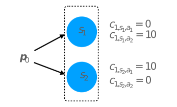
   Figure 9: Example of an Optimal Tree Policy instance where all optimal policies are dependent on $\bm{p}_{1}$, the initial distribution over the set of states. The same action has to be taken for the states in the region defined by the dashed rectangle.

   Assume that the set $\mathbb{T}$ of acceptable trees is such that for all tree $T\in\mathbb{T}$, the states $s_{1},s_{2}$ belong to the same class. In this case, the same action has to be taken in both $s_{1}$ and $s_{2}$. If the initial distribution $\bm{p}_{1}$ over $\{s_{1},s_{2}\}$ is $p_{1,s_{1}}=1,p_{1,s_{2}}=0$, then the optimal action to minimize the total cost is to choose action $a_{1}$. Otherwise, if the initial distribution $\bm{p}_{1}$ is $p_{1,s_{1}}=0,p_{1,s_{2}}=1$, then the optimal action to minimize the total cost is to choose action $a_{2}$. Therefore, the optimal policy depends of the initial distribution $\bm{p}_{1}$.

2. All optimal tree policies for $T$ may be history-dependent. The optimal decision rule $\pi_{t}$ chosen at period $t$ depends both on the value function $\bm{v}_{t+1}$ (i.e., on the decisions chosen after period $t$), but also on the distribution over the set of states $\mathbb{S}_{t}$, i.e., of what state the decision maker will reach at period $t$. This distribution depends on the previous decisions, i.e., it depends on $\pi_{1},...,\pi_{t-1}$. This is the reason why an optimal policy may be history dependent. In particular, we provide the following simple instance, which builds upon the previous example. We consider an Optimal Tree Policy instance where

   $$H=2,\mathbb{S}_{1}=\{s_{1},s^{\prime}_{1}\},\mathbb{A}_{1}=\{a_{1}\},\mathbb{S}_{2}=\{s_{2},s_{3},s_{4}\},\mathbb{A}_{2}=\{a_{2},a_{3}\}.$$

   

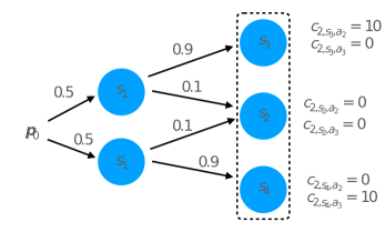
   Figure 10: Example of an Optimal Tree Policy instance where all optimal policies are history-dependent. The same action has to be taken for the states in the region defined by the dashed rectangle. There is no cost at $t=1$. The optimal policy at $t=2$ is dependent upon visiting $s_{1}$ or $s^{\prime}_{1}$ at $t=1$. The transitions probabilities are indicated above the transitions.

   There are two states $s_{1}$ and $s^{\prime}_{1}$ at $t=1$, and $p_{1,s_{1}}=p_{1,s^{\prime}_{1}}=0.5$. There is only one action $a_{1}$ in both $s_{1}$ and $s^{\prime}_{1}$ and the costs at $t=1$ are $c_{1,s_{1}a_{1}}=c_{1,s^{\prime}_{1}a_{1}}=0$. There are three states $s_{2},s_{3},s_{4}$ at period $t=2$ and all belong to the same class of the decision tree at $t=2$. Therefore, the same action has to be chosen in all three states. If the decision maker is in $s_{1}$ at period $t=1$, s/he transitions to $s_{3}$ with probability $0.9$ and to $s_{2}$ with probability $0.1$. If the decision maker is in $s^{\prime}_{1}$ at period $t=1$, s/he transitions to $s_{4}$ with probability $0.9$ and to $s_{2}$ with probability $0.1$.

   At period $t=2$, the costs are given by

   $$c_{2,s_{2},a_{2}}=0,c_{2,s_{2},a_{3}}=0,$$

   $$c_{2,s_{3},a_{2}}=10,c_{2,s_{3},a_{3}}=0,$$

   $$c_{2,s_{4},a_{2}}=0,c_{2,s_{4},a_{3}}=10.$$

   If the history prior to period $t=2$ is $(s_{1},a_{1})$, then the distribution over the states $(s_{2},s_{3},s_{4})$ visited at $t=2$ is $\left(0.1,0.9,0\right)$, and the optimal action at $t=2$ is to choose $a_{3}$. However, if the history prior to period $t=2$ is $(s^{\prime}_{1},a_{1})$, then the distribution over the states $(s_{2},s_{3},s_{4})$ visited at $t=2$ is $\left(0.1,0,0.9\right)$, and the optimal action at $t=2$ is to choose $a_{4}$. Therefore, we see that the optimal decision rule $\pi^{*}_{2}$ for period $t=2$ depends on the history prior to period $t=2$. The optimal policy, which is history-dependent, achieves a cost of $0$. Any Markovian (randomized or deterministic) policy which does not depend upon the state visited at $t=1$ will achieve a cost strictly higher than 0.

3. There always exists an optimal tree policy for $T$ that is deterministic (even though it may be history-dependent). We prove this statement by contradiction. Let us consider a sequence of trees $T$ for which all optimal policies are randomized, i.e., where for any optimal policy $\pi^{*}=\pi^{*}_{1},...,\pi^{*}_{H}$, there exists a period $t\in[1,H]$ such that $\pi^{*}_{t}$ is randomized. For each policy $\pi$, we call $t_{1}(\pi)\in[1,H]$ the first period $t$ where the decision rule $\pi_{t}$ is randomized.

   Let us consider $\pi^{*}$ the optimal policy where the period $t_{1}(\pi^{*})$ is as large as possible. Therefore, $\pi^{*}_{1},...,\pi^{*}_{t_{1}-1}$ are deterministic, but $\pi^{*}_{t_{1}}$ is randomized. We will construct an optimal policy $\pi^{\prime}$ where $\pi^{\prime}_{1},...,\pi^{\prime}_{t_{1}}$ are deterministic, resulting in a contradiction.

   In particular, let $\left(\pi^{\prime}_{1},...,\pi^{\prime}_{t_{1}-1}\right)=\left(\pi^{*}_{1},...,\pi^{*}_{t_{1}-1}\right)$. Therefore, the distribution on the set of states visited at period $t_{1}$ are the same for $\pi^{*}$ and for $\pi^{\prime}$, and the cumulative expected cost from period $t=1$ to period $t=t_{1}-1$ are the same.

   We call $\nu\in\Delta(\mathbb{S}_{t_{1}})$ the distribution on the set of states visited at period $t_{1}$, which is common to both $\pi^{*}$ and $\pi^{\prime}$. Let $C_{\sf tree,1\rightarrow t_{1}-1}$ the cumulative cost from period $t=1$ to period $t=t_{1}-1$, also common to both $\pi^{*}$ and $\pi^{\prime}$. We also choose $\left(\pi^{\prime}_{t_{1}+1},...,\pi^{\prime}_{H}\right)=\left(\pi^{*}_{t_{1}+1},...,\pi^{*}_{H}\right)$, i.e., $\pi^{\prime}$ is the same as $\pi^{*}$ from period $t_{1}+1$ to period $H$. Therefore, $v^{\pi^{*}}_{t_{1}+1,s}=v^{\pi^{\prime}}_{t_{1}+1,s},\forall\;s\in\mathbb{S}_{t_{1}+1}.$ We write $\bm{v}_{t_{1}+1}$ the vector $\bm{v}_{t_{1}+1}=\bm{v}^{\pi^{\prime}}_{t_{1}+1}$. Now let us choose $\pi^{\prime}_{t_{1}}$ in a deterministic way. In particular, we choose $\pi^{\prime}_{t_{1}}$ for period $t_{1}$ as the solution of

   $$\min_{\pi\in\Pi_{T}}\sum_{c\in[K_{t_{1}}]}\sum_{s\in\mathbb{S}_{t_{1}}}\nu_{s}\sum_{a\in\mathbb{A}_{t_{1}}}1_{\{T_{t_{1}}(s)=c\}}\pi_{sa}\left(r_{t_{1},sa}+\sum_{s^{\prime}\in\mathbb{S}_{t+1}}P_{t_{1},sas^{\prime}}v_{t_{1}+1,s^{\prime}}\right).$$

   Adding the constant $C_{\sf tree,1\rightarrow t_{1}-1}$, we see that $\pi^{\prime}_{t_{1}}$ minimizes

   $$\pi\mapsto C_{\sf tree,1\rightarrow t_{1}-1}+\sum_{c\in[K_{t_{1}}]}\sum_{s\in\mathbb{S}_{t_{1}}}\nu_{s}\sum_{a\in\mathbb{A}_{t_{1}}}1_{\{T_{t_{1}}(s)=c\}}\pi_{sa}\left(r_{t_{1},sa}+\sum_{s^{\prime}\in\mathbb{S}_{t+1}}P_{t_{1},sas^{\prime}}v_{t_{1}+1,s^{\prime}}\right),$$

   where $T$ is the tree chosen by $\pi^{*}$ for period $t_{1}$. Because $\bm{\nu}_{s}$ is the distribution over the states visited at period $t_{1}$ induced by both $\pi^{\prime}$ and $\pi^{*}$, and because $\bm{v}_{t_{1}+1}$ is the value function of both $\pi^{\prime}$ and $\pi^{*}$ after period $t_{1}$, we have that

   $$C_{\sf tree}(\pi^{\prime})=C_{\sf tree,1\rightarrow t_{1}-1}+\sum_{c\in[K_{t_{1}}]}\sum_{s\in\mathbb{S}_{t_{1}}}\nu_{s}\sum_{a\in\mathbb{A}_{t_{1}}}1_{\{T_{t_{1}}(s)=c\}}\pi^{\prime}_{t_{1},sa}\left(r_{t_{1},sa}+\sum_{s^{\prime}\in\mathbb{S}_{t+1}}P_{t_{1},sas^{\prime}}v_{t_{1}+1,s^{\prime}}\right).$$

   But this means that

   $$C_{\sf tree}(\pi^{\prime}) =C_{\sf tree,1\rightarrow t_{1}-1}+\sum_{c\in[K_{t_{1}}]}\sum_{s\in\mathbb{S}_{t_{1}}}\nu_{s}\sum_{a\in\mathbb{A}_{t_{1}}}1_{\{T_{t_{1}}(s)=c\}}\pi^{\prime}_{t_{1},sa}\left(r_{t_{1},sa}+\sum_{s^{\prime}\in\mathbb{S}_{t+1}}P_{t_{1},sas^{\prime}}v_{t_{1}+1,s^{\prime}}\right)$$

   $$\leq C_{\sf tree,1\rightarrow t_{1}-1}+\sum_{c\in[K_{t_{1}}]}\sum_{s\in\mathbb{S}_{t_{1}}}\nu_{s}\sum_{a\in\mathbb{A}_{t_{1}}}1_{\{T_{t_{1}}(s)=c\}}\pi^{*}_{t_{1},sa}\left(r_{t_{1},sa}+\sum_{s^{\prime}\in\mathbb{S}_{t+1}}P_{t_{1},sas^{\prime}}v_{t_{1}+1,s^{\prime}}\right)$$

   $$=C_{\sf tree}(\pi^{*}).$$

   Therefore, we constructed a policy $\pi^{\prime}$ with $C_{\sf tree}(\pi^{\prime})\leq C_{\sf tree}(\pi^{*})$. Since $\pi^{*}$ is an optimal policy, $\pi^{\prime}$ is also optimal. But $\pi^{\prime}_{1},...,\pi^{\prime}_{t_{1}}$ are all deterministic. Therefore, the first period where $\pi^{\prime}$ is randomized is higher than $t_{1}+1$, contradicting the assumption about $\pi^{*}$ and $t_{1}$. This concludes the proof.

∎

Appendix D Details on the New York State guidelines for triage and reassessment

In New York State (NYS), the Crisis Standards of Care guidelines were codified by the NYS Taskforce on Life and the Law in the 2015 Ventilator Triage Guidelines [Zucker et al., 2015]. These guidelines outline clinical criteria for triage, including exclusion criteria and stratification of patients using the Sequential Organ Failure Assessment (SOFA) score. We present these guidelines in a tree policy form in Figure 11. The goal of the NYS guidelines is to save the maximum number of lives. Note the important distinction with the number of life-years saved; age should only be used as a tie-breaker. In particular, the NYS does not use categorical exclusion of specific patients sub-populations, based on demographics (such as age, BMI) or comorbid health conditions (such as history of diabetes or congestive heart failures).

In particular, prior to reaching ventilator capacity constraint, ventilators are allocated first-come-first-served. When the capacity constraint is reached, new patients are triaged using SOFA scores:

• Those with SOFA $>$ 11 are categorized as blue (lowest priority) and do not receive a ventilator.

• Those with 1 $<$ SOFA $<$ 8 are categorized as red (highest priority) and receive a ventilator first.

• Those with SOFA between 8 and 11 are categorized as yellow (intermediate priority) and receive a ventilator as long as they are available and all patients in the red category have received a ventilator.

• Those with SOFA = 0 are categorized as green (lowest priority, same as blue) and do not receive a ventilator.

At 48 and 120 hours, patients on ventilators are re-assessed and categorized as blue (SOFA $>$ 11 or between 8 and 11 and not improving), yellow (SOFA $<$ 8 but not improving) or red (SOFA $<$ 8 and improving). Patients in blue and yellow categories are removed from the ventilator if a new patient with a higher priority requires one; patients in the blue category are removed first. In our representation of the NYS policies, we translate the priority classes blue and green as low priority, yellow as medium (med.) priority, and red as high priority.

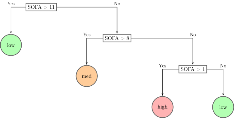
(a) Triage.

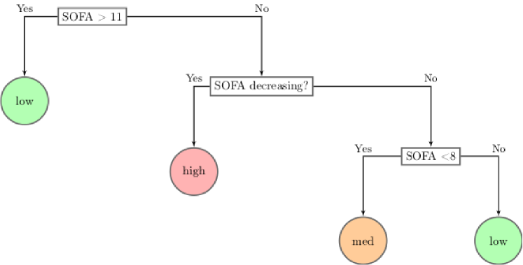
(b) Reassessment at t=48h.

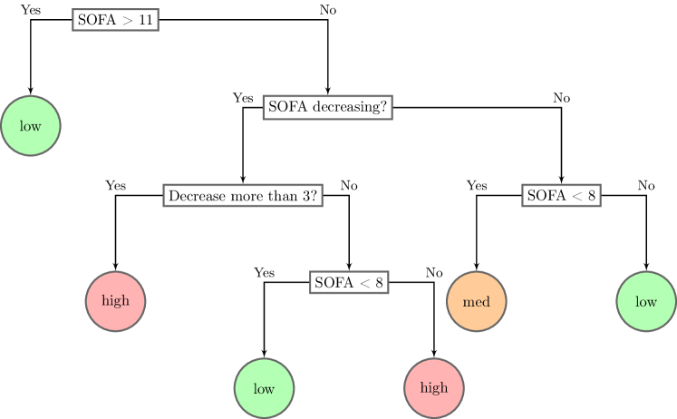
(c) Reassessment at t=120h.

Figure 11: Representation of the NYS guidelines as tree policies.

Appendix E Tree policies computed by our MDP model

We present here the tree policies that we computed with Algorithm 1. In Figure 12, the only covariates are SOFA and whether the SOFA is decreasing or increasing (compared to intubation or last reassessment). In Figure 13, the covariates are SOFA, SOFA decreasing or increasing, and age. In Figure 14, the covariates are SOFA, SOFA decreasing or increasing, age, the Charlson score, BMI, the presence of malignancy, metastatic solid tumor, diabetes with or without chronic complications, dementia, congestive heart failure, AIDS/HIV, moderate or severe liver disease. Note that the final tree in Figure 14 only uses SOFA and SOFA decreasing or increasing, age, and BMI.

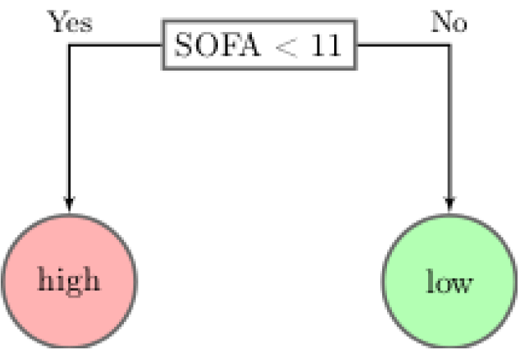
(a) Triage.

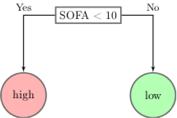
(b) Reassessment at t=48h.

(c) Reassessment at t=120h.

Figure 12: Tree policies only based on SOFA.

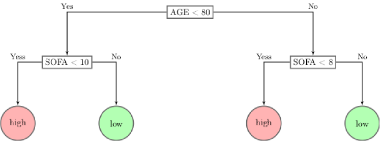
(a) Triage.

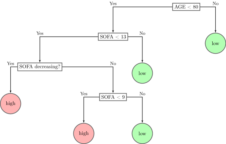
(b) Reassessment at t=48h.

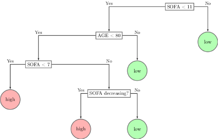
(c) Reassessment at t=120h.

Figure 13: Tree policies based on SOFA and age.

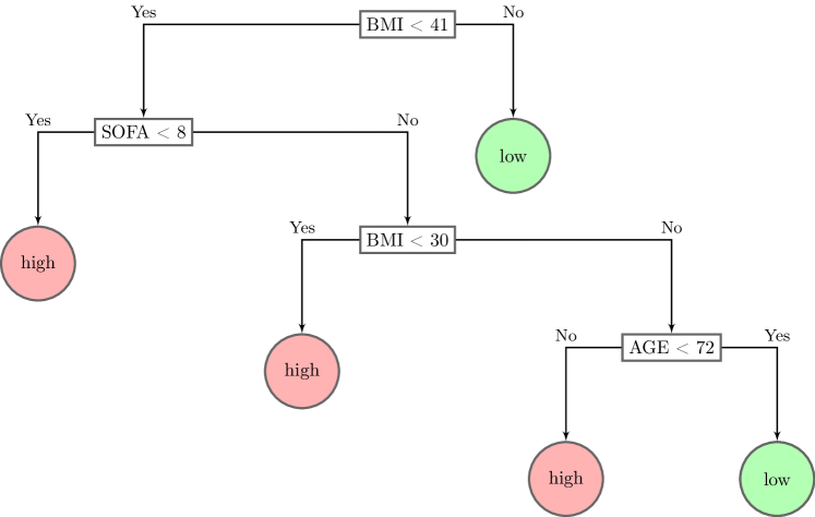
(a) Triage.

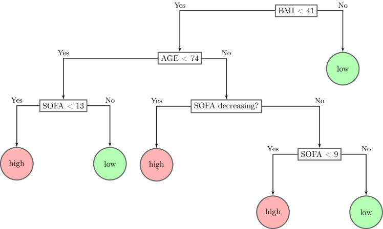
(b) Reassessment at t=48h.

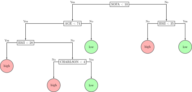
(c) Reassessment at t=120h.

Figure 14: Tree policies using SOFA and other covariates.

Appendix F Number of deaths with other values of $p$

We present our numerical results for $p\in\{0.50,0.70,0.90\}$ in Figure 15(a)-15(c). Recall that $p$ is a proxi for the chance of dying for patients that are excluded from ventilator treatment.

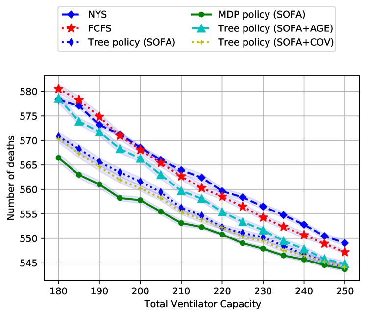
(a) $p=0.90$.

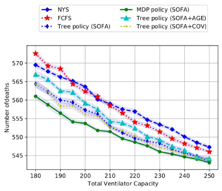
(b) $p=0.70$.

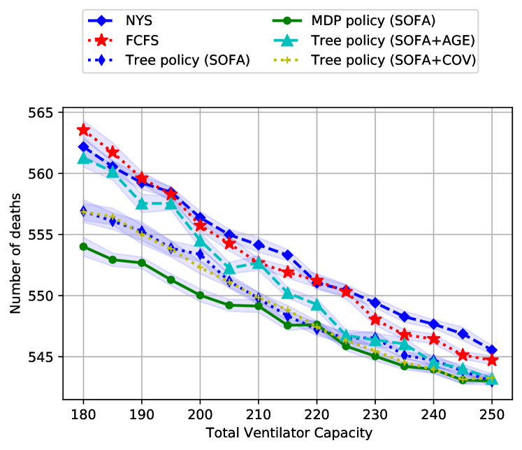
(c) $p=0.50$.

Figure 15: Estimated number of deaths for $p\in\{0.90,0.70,0.50\}.$

Appendix G Sensitivity analysis for the costs parameters

In this appendix we present a sensitivity analysis as regards the costs parameters for the MDP. In particular, in the empirical results of Section 5, we have chosen $C=100,\rho=1.1,\gamma=1.5$, we computed optimal policies and tree policies, and estimated their performances using our simulation model from Section 5.1. Here, we vary the parameters $C,\rho$ and $\gamma$ and estimate again the performances of the tree policies (computed with Algorithm 1). Because we are already varying $3$ parameters, we only show here the variations in the number of deaths at a capacity $180$ ventilators, for the policies only relying on SOFA. We observe similar results for other ventilator capacities in $[180,250]$ and for the policies relying on SOFA and age, and SOFA and covariates.

Recall that we maintain $C/\gamma>\gamma\rho^{2}$, so that the “best” state for deceased patients ($D_{1}^{ex}$, with cost $C/\gamma$) has higher cost than the “worse” state for patients discharged alive ($A^{ex}_{3}$, with cost $\gamma\rho^{2}$). In our sensitivity analysis we vary $\gamma\in[1,5]$ and $\rho\in[1,5]$, using steps of $0.2$. Note that $\rho=5$ corresponds to an extreme actualization factor, e.g., the cost is multiplied by $25$ after only two periods. This is the reason why we choose to stop at $\rho=5$. The same holds for $\gamma$. For each pair $\gamma,\rho$, we vary $C$ in $[\gamma^{2}\rho^{2}+5,\gamma^{2}\rho^{2}+65]$ using steps of $10$. This way, we always maintain $C/\gamma>\gamma\rho^{2}$.

We find that for $\gamma\in[1,5],\rho\in[1,4.8],C\in[\gamma^{2}\rho^{2}+5,\gamma^{2}\rho^{2}+65]$, the tree policies computed by Algorithm 1 do not change. For $\rho=5$, the tree policies vary, with tree policies corresponding to $\gamma$ close to $1$ and $C$ close to $\gamma^{2}\rho^{2}+100$ being closer to the original trees computed in the main body of the algorithm with $C=100,\rho=1.1,\gamma=1.5$. In particular, when we have $C=\gamma^{2}\rho^{2}+10$ and $\rho=5$, we see very poor performances of the tree policies. This can be noticed in Figure 16(a) and Figure 16(b) for various values of $\gamma$. This is mostly because the costs for deceased states are too close to the costs for states corresponding to patients alive at discharge, i.e. that $C/\gamma$ is too close to $\gamma\rho^{2}$, which in turn means that the MDP formulation is pointless for our purpose of minimizing the number of patients who die. When $C$ increases again, the performances of the computed tree policies become closer to the performances of the tree policies computed for $C=100,\rho=1.1,\gamma=1.5$. Therefore, we recommend to choose $C,\rho$ and $\gamma$ such that $C/\gamma$ is significantly larger than $\gamma\rho^{2}$. We want to note that the best tree policies (in terms of number of patients saved) among all the choices of $C,\gamma,\rho$ that we tested correspond to the trees that we have computed with $C=100,\rho=1.1,\gamma=1.5$.

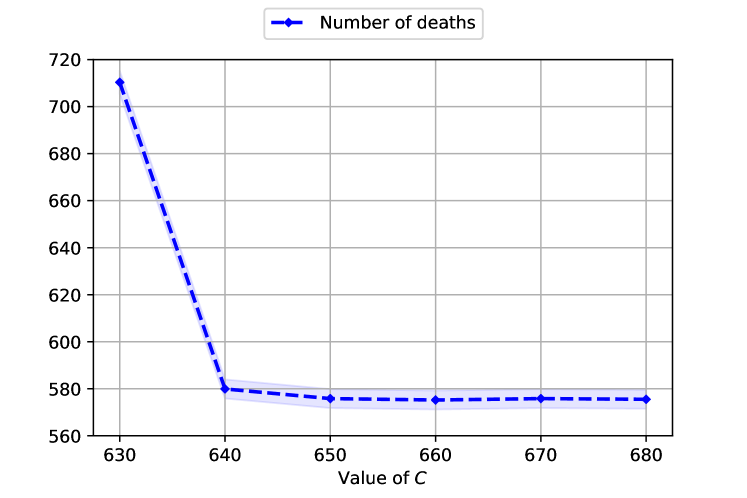
(a) $\rho=5,\gamma=5$.

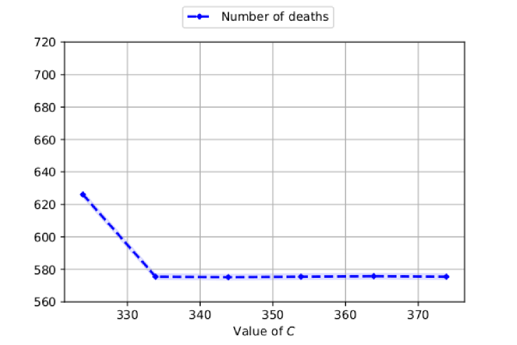
(b) $\rho=5,\gamma=3.5$.

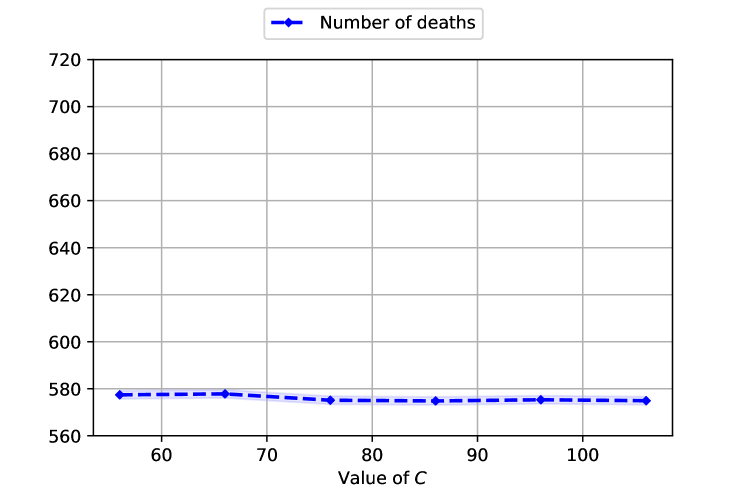
(c) $\rho=5,\gamma=1.5$.

Figure 16: Estimated number of deaths for the tree policies computed with various values of the parameters $\rho,\gamma,C$. We always consider $C$ such that $C/\gamma\geq\gamma\rho^{2}$.

Appendix H Details about the clinical data set

Summary statistics for our cohort of patients are presented in Table 1.

Variables	All population	Survived	Deceased
Number (n)	807	264	543
Age (year (std))	64.0 (13.5)	60.0 (13.1)	66.4 (12.9)
Male gender (n (%))	483 (59.9 %)	132 (50 %)	351 (64.6 %)
BMI (mean (std))	30.8 (7.5)	30.7 (7.2)	30.8 (7.7)
Diabetes (n (%))	319 (40.0 %)	78 (30.0 %)	241 (44.4 %)
Charlson (mean (std))	2.9 (2.7)	2.0 (2.6)	3.3 (2.7)
Malignancy (n (%))	39 (4.5 %)	4 (1.5 %)	35 (6.5 %)
Renal disease (n (%))	341 (42.2 %)	66 (25.0 %)	275 (50.7 %)
Dementia (n (%))	92 (11.4 %)	23 (8.7 %)	69 (12.7 %)
Congestive Heart Failure (n )%))	149 (18.5 %)	26 (9.9 %)	123 (22.7 %)
Initial SOFA (mean (IQR))	2.0 (0.0-3.0)	1.5 (0.0-2.0)	2.2 (0.0-3.0)
Max SOFA (mean (IQR))	9.7 (8.0-12.0)	8.5 (7.0-10.0)	10.2 (8.0-12.0)
LOS (median (IQR))	16.8 (8.7-29.2)	29.1 (18.9-46.5)	12.5 (6.9-21.0)
Survival (n (%))	264 (32.7 %)	$\cdot$	$\cdot$

Table 1: Summary statistics for the patients in our data set.

References

- Adelman and Mersereau [2008] Daniel Adelman and Adam J Mersereau. Relaxations of weakly coupled stochastic dynamic programs. Operations Research, 56(3):712–727, 2008.
- Alagoz et al. [2004] Oguzhan Alagoz, Lisa M Maillart, Andrew J Schaefer, and Mark S Roberts. The optimal timing of living-donor liver transplantation. Management Science, 50(10):1420–1430, 2004.
- Alagoz et al. [2010] Oguzhan Alagoz, Heather Hsu, Andrew J Schaefer, and Mark S Roberts. Markov decision processes: a tool for sequential decision making under uncertainty. Medical Decision Making, 30(4):474–483, 2010.
- Alizamir et al. [2013] Saed Alizamir, Francis De Véricourt, and Peng Sun. Diagnostic accuracy under congestion. Management Science, 59(1):157–171, 2013.
- Amin and Ali [2018] M Amin and Amir Ali. Performance evaluation of supervised machine learning classifiers for predicting healthcare operational decisions. Wavy AI Research Foundation: Lahore, Pakistan, 2018.
- Anderson et al. [2021] David Anderson, Tolga Aydinliyim, Margret Bjarnadottir, Eren Cil, and Michaela Anderson. Rationing scarce healthcare capacity: A study of the ventilator allocation guidelines during the COVID-19 pandemic in the United States. Available at SSRN 3797325, 2021.
- Argon and Ziya [2009] Nilay Tanık Argon and Serhan Ziya. Priority assignment under imperfect information on customer type identities. Manufacturing & Service Operations Management, 11(4):674–693, 2009.
- Auriemma et al. [2020] Catherine L Auriemma, Ashli M Molinero, Amy J Houtrow, Govind Persad, Douglas B White, and Scott D Halpern. Eliminating categorical exclusion criteria in crisis standards of care frameworks. The American Journal of Bioethics, 20(7):28–36, 2020.
- Babar and Rinker [2016] I Babar and R Rinker. Direct patient care during an acute disaster: chasing the will-o’-the-wisp. Critical care (London, England), 10:206, 2016.
- Bakker and Tsui [2017] Monique Bakker and Kwok-Leung Tsui. Dynamic resource allocation for efficient patient scheduling: A data-driven approach. Journal of Systems Science and Systems Engineering, 26(4):448–462, 2017.
- Beauchamp et al. [2001] Tom L Beauchamp, James F Childress, et al. Principles of biomedical ethics. Oxford University Press, USA, 2001.
- Beck and Pauker [1983] J Robert Beck and Stephen G Pauker. The Markov process in medical prognosis. Medical decision making, 3(4):419–458, 1983.
- Bertsimas et al. [2011] D. Bertsimas, D.B. Brown, and C. Caramanis. Theory and applications of robust optimization. SIAM review, 53(3):464–501, 2011.
- Bertsimas and Dunn [2017] Dimitris Bertsimas and Jack Dunn. Optimal classification trees. Machine Learning, 106(7):1039–1082, 2017.
- Bertsimas et al. [2020] Dimitris Bertsimas, Jack Dunn, Emma Gibson, and Agni Orfanoudaki. Optimal survival trees. arXiv preprint arXiv:2012.04284, 2020.
- Bravo and Shaposhnik [2020] Fernanda Bravo and Yaron Shaposhnik. Mining optimal policies: A pattern recognition approach to model analysis. INFORMS Journal on Optimization, 2(3):145–166, 2020.
- Breiman et al. [1984] Leo Breiman, Jerome Friedman, Charles J Stone, and Richard A Olshen. Classification and regression trees. CRC press, 1984.
- Bunch [2021] Lauren Bunch. A tale of two crises: Addressing COVID-19 vaccine hesitancy as promoting racial justice. In HEC forum, volume 33, pages 143–154. Springer, 2021.
- Chan et al. [2012] Carri W Chan, Vivek F Farias, Nicholas Bambos, and Gabriel J Escobar. Optimizing intensive care unit discharge decisions with patient readmissions. Operations research, 60(6):1323–1341, 2012.
- Chan et al. [2013] Carri W Chan, Linda V Green, Yina Lu, Nicole Leahy, and Roger Yurt. Prioritizing burn-injured patients during a disaster. Manufacturing & Service Operations Management, 15(2):170–190, 2013.
- Chen et al. [2020] Wanyi Chen, Benjamin Linthicum, Nilay Tanik Argon, Thomas Bohrmann, Kenneth Lopiano, Abhi Mehrotra, Debbie Travers, and Serhan Ziya. The effects of emergency department crowding on triage and hospital admission decisions. The American journal of emergency medicine, 38(4):774–779, 2020.
- Childers et al. [2009] Ashley Kay Childers, Gurucharann Visagamurthy, and Kevin Taaffe. Prioritizing patients for evacuation from a health-care facility. Transportation research record, 2137(1):38–45, 2009.
- Christian et al. [2014] Michael D Christian, Charles L Sprung, Mary A King, Jeffrey R Dichter, Niranjan Kissoon, Asha V Devereaux, and Charles D Gomersall. Triage: care of the critically ill and injured during pandemics and disasters: Chest consensus statement. Chest, 146(4):e61S–e74S, 2014.
- Chuang et al. [2021] Elizabeth Chuang, Julien Grand-Clement, Jen-Ting Chen, Carri W Chan, Vineet Goyal, and Michelle Ng Gong. Quantifying utilitarian outcomes to inform triage ethics: Simulated performance of a ventilator triage protocol under sars-cov-2 pandemic surge conditions. Available at SSRN 3901764, 2021.
- Ciocan and Mišić [2020] Dragos Florin Ciocan and Velibor V Mišić. Interpretable optimal stopping. Management Science, 2020.
- Cockerham et al. [2017] William C Cockerham, Bryant W Hamby, and Gabriela R Oates. The social determinants of chronic disease. American journal of preventive medicine, 52(1):S5–S12, 2017.
- Dhillon and Singh [2019] Arwinder Dhillon and Ashima Singh. Machine learning in healthcare data analysis: A survey. Journal of Biology and Today’s World, 8(6):1–10, 2019.
- Dobson and Sainathan [2011] Gregory Dobson and Arvind Sainathan. On the impact of analyzing customer information and prioritizing in a service system. Decision Support Systems, 51(4):875–883, 2011.
- Frykberg [2005] Eric R Frykberg. Triage: principles and practice. Scandinavian Journal of Surgery, 94(4):272–278, 2005.
- Gershengorn et al. [2021] Hayley B Gershengorn, Yue Hu, Jen-Ting Chen, S Jean Hsieh, Jing Dong, Michelle Ng Gong, and Carri W Chan. The impact of high-flow nasal cannula use on patient mortality and the availability of mechanical ventilators in COVID-19. Annals of the American Thoracic Society, 18(4):623–631, 2021.
- Gostin et al. [2012] Lawrence O Gostin, Kristin Viswanathan, Bruce M Altevogt, Dan Hanfling, et al. Crisis standards of care: A systems framework for catastrophic disaster response. 2012.
- Goyal and Grand-Clément [2018] Vineet Goyal and Julien Grand-Clément. Robust Markov Decision Process: Beyond Rectangularity. ArXiv e-prints, 2018. URL https://arxiv.org/abs/1811.00215.
- Grand-Clément et al. [2020] Julien Grand-Clément, Carri W Chan, Vineet Goyal, and Gabriel Escobar. Robust policies for proactive ICU transfers. arXiv preprint arXiv:2002.06247, 2020.
- Grand-Clément et al. [2021] Julien Grand-Clément, V Goyal, CW Chan, MN Gong, EC Chuang, J-T Chen, and P Cuartas. Estimation of excess mortality resulting from use of a ventilator triage protocol under sars-cov-2 pandemic surge conditions. In TP50. TP050 COVID: NONPULMONARY CRITICAL CARE, MECHANICAL VENTILATION, BEHAVIORAL SCIENCES, AND EPI, pages A2589–A2589. American Thoracic Society, 2021.
- Hwang and Bedrosian [2014] E Shelley Hwang and Isabelle Bedrosian. Patterns of breast magnetic resonance imaging use: an opportunity for data-driven resource allocation. JAMA internal medicine, 174(1):122–124, 2014.
- Iyengar [2005] G. Iyengar. Robust dynamic programming. Mathematics of Operations Research, 30(2):257–280, 2005.
- Jacobson et al. [2012] Evin Uzun Jacobson, Nilay Tanık Argon, and Serhan Ziya. Priority assignment in emergency response. Operations Research, 60(4):813–832, 2012.
- Jones et al. [2009] Alan E Jones, Stephen Trzeciak, and Jeffrey A Kline. The sequential organ failure assessment score for predicting outcome in patients with severe sepsis and evidence of hypoperfusion at the time of emergency department presentation. Critical care medicine, 37(5):1649, 2009.
- Khan et al. [2008] Muhammad Umer Khan, Jong Pill Choi, Hyunjung Shin, and Minkoo Kim. Predicting breast cancer survivability using fuzzy decision trees for personalized healthcare. In 2008 30th annual international conference of the IEEE engineering in medicine and biology society, pages 5148–5151. IEEE, 2008.
- Kim et al. [2015] Song-Hee Kim, Carri W Chan, Marcelo Olivares, and Gabriel Escobar. ICU admission control: An empirical study of capacity allocation and its implication for patient outcomes. Management Science, 61(1):19–38, 2015.
- Kotnala et al. [2021] Rajeev K Kotnala, Deepak K Tempe, Prashant Mishra, Siddarth Ramji, and Amaresh P Patil. Clinical triage in a large 2000-bed COVID-19 care facility: Role of the anesthesiologist. Journal of Cardiothoracic and Vascular Anesthesia, 2021.
- Laurent and Rivest [1976] Hyafil Laurent and Ronald L Rivest. Constructing optimal binary decision trees is NP-complete. Information processing letters, 5(1):15–17, 1976.
- Li and Glazebrook [2010] Dong Li and Kevin D Glazebrook. An approximate dynamic programing approach to the development of heuristics for the scheduling of impatient jobs in a clearing system. Naval Research Logistics (NRL), 57(3):225–236, 2010.
- May and Aulisio [2020] Thomas May and Mark P Aulisio. Age,“life-cycles,” and the allocation of scarce medical resources. Chest, 158(5):1837–1838, 2020.
- Mello et al. [2020] Michelle M Mello, Govind Persad, and Douglas B White. Respecting disability rights—toward improved crisis standards of care. New England Journal of Medicine, 383(5):e26, 2020.
- Mills et al. [2013] Alex F Mills, Nilay Tanık Argon, and Serhan Ziya. Resource-based patient prioritization in mass-casualty incidents. Manufacturing & Service Operations Management, 15(3):361–377, 2013.
- Orfanoudaki et al. [2020] Agni Orfanoudaki, Emma Chesley, Christian Cadisch, Barry Stein, Amre Nouh, Mark J Alberts, and Dimitris Bertsimas. Machine learning provides evidence that stroke risk is not linear: The non-linear Framingham stroke risk score. PloS one, 15(5):e0232414, 2020.
- Orioli et al. [2020] Laura Orioli, Michel P Hermans, Jean-Paul Thissen, Dominique Maiter, Bernard Vandeleene, and Jean-Cyr Yombi. COVID-19 in diabetic patients: Related risks and specifics of management. In Annales d’endocrinologie, volume 81, pages 101–109. Elsevier, 2020.
- Piscitello et al. [2020] Gina M Piscitello, Esha M Kapania, William D Miller, Juan C Rojas, Mark Siegler, and William F Parker. Variation in ventilator allocation guidelines by US state during the coronavirus disease 2019 pandemic: a systematic review. JAMA network open, 3(6):e2012606–e2012606, 2020.
- Puterman [1994] M.L. Puterman. Markov Decision Processes : Discrete Stochastic Dynamic Programming. John Wiley and Sons, 1994.
- Quinlan [2014] J Ross Quinlan. C4. 5: programs for machine learning. Elsevier, 2014.
- Rosenbaum [2020] Lisa Rosenbaum. Facing COVID-19 in italy—ethics, logistics, and therapeutics on the epidemic’s front line. New England Journal of Medicine, 382(20):1873–1875, 2020.
- Rudin [2019] Cynthia Rudin. Stop explaining black box machine learning models for high stakes decisions and use interpretable models instead. Nature Machine Intelligence, 1(5):206–215, 2019.
- Sacco et al. [2007] William J Sacco, D Michael Navin, Robert K Waddell, Katherine E Fiedler, William B Long, Robert F Buckman Jr, et al. A new resource-constrained triage method applied to victims of penetrating injury. Journal of Trauma and Acute Care Surgery, 63(2):316–325, 2007.
- Shechter et al. [2008] Steven M Shechter, Matthew D Bailey, Andrew J Schaefer, and Mark S Roberts. The optimal time to initiate HIV therapy under ordered health states. Operations Research, 56(1):20–33, 2008.
- Shouman et al. [2011] Mai Shouman, Tim Turner, and Rob Stocker. Using decision tree for diagnosing heart disease patients. In Proceedings of the Ninth Australasian Data Mining Conference-Volume 121, pages 23–30, 2011.
- Steimle and Denton [2017] Lauren N Steimle and Brian T Denton. Markov decision processes for screening and treatment of chronic diseases. In Markov Decision Processes in Practice, pages 189–222. Springer, 2017.
- Sun et al. [2018] Zhankun Sun, Nilay Tanık Argon, and Serhan Ziya. Patient triage and prioritization under austere conditions. Management Science, 64(10):4471–4489, 2018.
- Sun et al. [2019] Zhankun Sun, Nilay Argon, and Serhan Ziya. When to triage in service systems with hidden customer class identities? Available at SSRN 3346173, 2019.
- Tomar and Agarwal [2013] Divya Tomar and Sonali Agarwal. A survey on data mining approaches for healthcare. International Journal of Bio-Science and Bio-Technology, 5(5):241–266, 2013.
- Van Mieghem [1995] Jan A Van Mieghem. Dynamic scheduling with convex delay costs: The generalized c/mu rule. The Annals of Applied Probability, pages 809–833, 1995.
- White and Lo [2020] Douglas B White and Bernard Lo. A framework for rationing ventilators and critical care beds during the covid-19 pandemic. Jama, 323(18):1773–1774, 2020.
- Whitt [2002] Ward Whitt. Stochastic-process limits: an introduction to stochastic-process limits and their application to queues. Springer Science & Business Media, 2002.
- Wiesemann et al. [2013] W. Wiesemann, D. Kuhn, and B. Rustem. Robust Markov decision processes. Operations Research, 38(1):153–183, 2013.
- Woodward and Samet [2018] AJ Woodward and JM Samet. Climate change, hurricanes, and health. Am J Public Health, 1(108):33–35, 2018.
- Wunsch et al. [2020] Hannah Wunsch, Andrea D Hill, Nicholas Bosch, Neill KJ Adhikari, Gordon Rubenfeld, Allan Walkey, Bruno L Ferreyro, Bourke W Tillmann, Andre CKB Amaral, Damon C Scales, et al. Comparison of two triage scoring guidelines for allocation of mechanical ventilators. JAMA network open, 3(12):e2029250–e2029250, 2020.
- Zhou et al. [2020] Fei Zhou, Ting Yu, Ronghui Du, Guohui Fan, Ying Liu, Zhibo Liu, Jie Xiang, Yeming Wang, Bin Song, Xiaoying Gu, et al. Clinical course and risk factors for mortality of adult inpatients with COVID-19 in Wuhan, China: a retrospective cohort study. The lancet, 395(10229):1054–1062, 2020.
- Zucker et al. [2015] HA Zucker, KP Adler, DP Berens, RJD Bleich, R Brynner, KA Butler, et al. Ventilator allocation guidelines. New York State task force on life and the law; 2015, 2015.
- Zumla et al. [2016] A Zumla, AN Alagaili, M Cotten, and EI Azhar. Infectious diseases epidemic threats and mass gatherings: refocusing global attention on the continuing spread of the middle east respiratory syndrome coronavirus (MERS-CoV). BMC medicine, 14:132, 2016.