A Decentralized Framework for Serverless Edge Computing in the Internet of Things

Abstract

Serverless computing is becoming widely adopted among cloud providers, thus making increasingly popular the Function-as-a-Service (FaaS) programming model, where the developers realize services by packaging sequences of stateless function calls. The current technologies are very well suited to data centers, but cannot provide equally good performance in decentralized environments, such as edge computing systems, which are expected to be typical for Internet of Things (IoT) applications. In this paper, we fill this gap by proposing a framework for efficient dispatching of stateless tasks to in-network executors so as to minimize the response times while exhibiting short- and long-term fairness, also leveraging information from a virtualized network infrastructure when available. Our solution is shown to be simple enough to be installed on devices with limited computational capabilities, such as IoT gateways, especially when using a hierarchical forwarding extension. We evaluate the proposed platform by means of extensive emulation experiments with a prototype implementation in realistic conditions. The results show that it is able to smoothly adapt to the mobility of clients and to the variations of their service request patterns, while coping promptly with network congestion.

I Introduction

Edge computing is a consolidated type of network deployment where the execution of services is pushed as close as possible to the user devices. This allows to achieve faster response times, relieve user devices from computationally-intensive tasks, reduce energy consumption, and lower traffic requirements, compared to current solutions where applications run fully on user devices or in a remote data center [5]. The Internet of Things (IoT) and mobile network domains are expected to gain maximum benefit from edge computing [28, 29], for which tangible commitments from industry are the reference architecture published by the OpenFog Consortium [27] and the interfaces and protocols for an inter-operable Multi-access Edge Computing (MEC) standardized within European Telecommunications Standards Institute (ETSI) [34].

Unrelated from edge computing, serverless is emerging among the cloud technologies to hide completely to the developer the notion of an underlying server (hence its name) and provide a true pay-per-use model with fine granularity [6]. To deliver this promise, a serverless platform must provide infinite scalability, achieved through a flexible up-/down-scaling of lean virtualisation abstractions (typically, containers). This has led to the widespread adoption of the Function as a Service (FaaS) programming model, where the application does not run as a whole process, but rather it is split into short-lived stateless tasks that can be executed by different workers without a tight coordination [17]. It is expected that serverless computing will become widespread in the future [20]. The seamless adoption of a FaaS paradigm in an edge system would allow to re-use applications, on both the provider’s and the user’s side, which were designed originally for serverless computing and are growing significantly in number and importance [26].

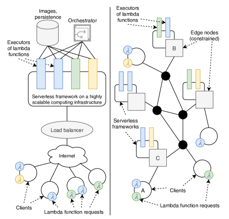
Figure 1: Serverless computing on a distributed (left) vs. edge (right) environment.

However, a straightforward deployment of serverless frameworks in an edge computing domain may not always be possible because of their different characteristics [15]. We elaborate on this point in the following with the help of the examples in Fig. 1. On the left part, we show a typical (simplified) set up of a serverless system, inspired from the architecture of Apache OpenWhisk. Generally, the core of the framework is a flexible container-based virtualization system hosted in a data center (i.e., operated by a single entity and running on high-end servers with fast connectivity), which is controlled by an orchestrator so that the number of executors matches the current demands from clients. The executors are the applications that respond to the requests of task executions, also called lambda functions. A load balancer at the ingress of the serverless system dispatches the incoming lambda functions towards the executors currently deployed. A database is represented in the figure to offer a repository of container images to be dynamically deployed, a persistence service, user credentials, etc. Overall, serverless systems can be considered viable implementations of many distributed computing models, such as Bulk Synchronous Parallel (BSP) as elaborated in [18].

In this work we focus instead on a different scenario where: (i) the tasks are executed by devices (edge nodes) with limited computation capabilities, such as WiFi access points or IoT gateways; (ii) these devices have limited connectivity towards a remote data center, which makes it impractical to realize vertical offloading, i.e., delegation to the cloud of the execution of tasks currently exceeding the capacity of an individual edge node; (iii) the clients are interspersed with edge nodes, i.e., there is no single point of access for all the users in the system. An example of our target system is illustrated in the right part of Fig. 1 and, in its essence, is also the subject of investigation in [16], where the authors envision that every edge node (or small cluster of edge nodes) hosts a serverless platform with state-of-the-art technology (e.g., every cluster may run an OpenWhisk instance). This allows to realize horizontal offloading, where delegation of task execution happens from one serverless platform to another in the edge network, thus achieving resource pooling at the edge, without resorting to the cloud. In this work we embrace this vision, and focus on the specific issue of distributing lambda function requests from clients to executors on the various serverless platforms available, which can be also heterogeneous in hardware/software and owned by different entities.

Note that this operation is different from the orchestration of multiple executors in a flexible computation infrastructure, as in a traditional serverless platform on cloud resources. First, despite some initial enthusiastic experiments with container clusters on constrained devices, such as K8s on Raspberry Pi’s [21], the high overhead and the orchestration system being designed for a very different target make such deployments unsuitable for a production system, as demonstrated in [8] for real-time 5G applications and in [30] for edge AI. Second, the lack of a natural point for the installation of a system-wide collector makes it inefficient to use a standard load balancer, such as NGINX, unless the edge operator is willing to pay the price of traversing multiple times the same link: e.g., with reference to Fig. 1, if the load balancer is installed in B, then lambda requests from A executed on C would have to unnecessarily traverse twice all the links between B and C, which could be unacceptable in many cases.

To overcome these limitations, in [9] we have first proposed a decentralized architecture, as opposed to the distributed approach of traditional serverless frameworks, which is illustrated for completeness in Sec. III. Briefly, the edge nodes providing user devices with network access (which we call edge routers — e-routers, defined in Sec. III) take autonomous decisions on where to forward the incoming lambda request, among the possible executors of matching type (which we call edge computers — e-computers, defined in Sec. III). To achieve fast processing rate on e-routers with limited capabilities we split this decision into two sub-functions, called weight updating and destination selection, by analogy with routing in Internet Protocol (IP) networks, which happens autonomously at each router (fast decision, called forwarding), but exploits cost information collected from routing protocols at much longer time scales.

In the same work [9], we have also outlined algorithms for the realization of these sub-functions. Weight updating is done by each e-router by measuring a smoothed average of every lambda function response time towards any e-computer, and avoiding paths indicated as congested by a Software Defined Networking (SDN) controller supervising the network layer (see Sec. IV-A). For destination selection, we consider three policies (well-known in the literature) to show that our framework is flexible enough to incorporate algorithms with different objective functions to fit specific use cases, which are evaluated according tot their short- and long-term fairness in Sec. IV-B. We assess the scalability of our solution in Sec. V. Specifically, by means of testbed experiments, we show that performance may be impaired as the number of services in the edge computing domain grows, but overcome this issue by enabling a hierarchical structure: an e-router may appear as an e-computer to other e-routers so as to receive lambda function requests, which it dispatches to nearby e-computers that were not addressable directly by other e-routers.

Finally, a comprehensive evaluation is carried out in an emulated environment, also integrating OpenWhisk platforms. The results, reported in Sec. VI, show that: (i) the interaction with the SDN controller is beneficial to relieve user applications from network congestion; (ii) our decentralized architecture is effective in following load variations in several conditions, and can achieve almost same performance as a distributed system with equivalent aggregate capacity; (iii) the system can achieve scalability, even with low-end edge nodes, by means of hierarchical forwarding. Our framework is available as open source.

II State of the art

The adoption of the serverless and FaaS paradigms in an edge environment has been first proposed by Baresi et. al, who have analyzed the issues and proposed high-level directions in their works. Among them, [4] is particularly relevant. In addition to providing a convincing motivation, which is fully aligned with our view expressed in Sec. I, they envision different types of deployment, all with multiple serverless platforms scattered in the network, depending on specific IoT use cases. Furthermore, they provide a detailed architecture of such platforms, supported by a prototype realized with OpenWhisk and other open source products. In this work we complement this result by defining a framework for the distribution of stateless tasks among the platforms, which has remained so far unspecified.

In a more general sense, the topic of edge computing has been already investigated broadly in the scientific literature, see for instance the survey [23]. In the following we report the state-of-the-art contributions that are most relevant to the topic addressed in this work.

On the one hand, solutions to the so-called edge-cloud problem have been proposed: how to dynamically dispatch jobs to a network of edge nodes based on the application requirements and the current load on the servers doing the computations [35], [14], [1], [7], thus realizing vertical offloading (as defined in Sec. I). Different from our work, these architectural approaches assume that (i) either the edge nodes are a geographic extension of the data centers, hence they are as much stable and dependable, and deployed in limited numbers, or (ii) the offloaded tasks are long-lived, thus it is suitable to assign tasks to edge nodes by solving a system-wide optimisation problem. Furthermore, they do not exploit integration with underlying SDN facilities, which is instead generally considered beneficial and it has been investigated in several research works, see for instance the survey in [3]. On the other hand, several works have proposed a lightweight orchestration, by scaling down cloud-oriented paradigms to less powerful servers and faster dynamics. Examples include Picasso [22], from which we reuse the concept of providing the applications with an Application Programming Interface (API) whose routines are executed by the network in a transparent manner to clients, and foglets [32], based on containers for an easier and faster migration of functions based on situation-awareness schemes. Both studies put forward efficient ways to periodically tune the deployment of Virtual Machines/containers in edge computers, which are out of the scope of the current work. On the other hand, some recent works have recently revamped the topic of distributed scheduling of “tasklets” ($\simeq$ lambdas) to realize complex applications with shared computational resources. In [13] the authors propose a way to reduce the number of tasklet execution failures, which stems from the high unreliability of the users offering computational resources. This is not applicable to the case under study where the edge nodes can safely be assumed to disconnect or fail very sporadically. Instead, a middleware is put forward in [33] to orchestrate tasklets through brokers, thus building a hybrid peer-to-peer network; however, the architecture is completely unaware of the underlying network and, in particular, does not collaborate with SDN functions as we propose.

With specific reference to edge computing environments, in [25] the authors propose an abstraction called Software-Defined Gateway, which hides the complexity of local IoT devices and offers a clean API for the integration with widely adopted serverless platforms; they focus on the DevOps aspects, and mention the issue of “scheduling [the] functions execution on loosely coupled and scarce edge resources” as an open research issue, which we address in this work. In [12] the authors take a more radical approach and assume that every edge node may decide at the same time where to route every incoming task (at a network-level) and which node has to execute the remaining processing, where applications are assumed to be modeled as directed computation graphs. In this setting they find theoretical results on the system stability, provided that the edge nodes employ a form of back-pressure, i.e., basically they take distributed decisions based on the length of their backlog queues. The approach is interesting and, even though we could not reuse the same exact methodology because of the different assumptions about the target system, we have inspired from the results in [12] to define the Round-robin algorithm, defined and analyzed in Sec. IV-B. Furthermore, in [11] we have proposed a solution to estimate the lambda execution time using real-time measurements from the executors, but this technique cannot be employed when e-routers are hosted on low-power IoT gateways due to the relatively high memory and computation requirements. Finally, in [2] the authors investigate the issue of decentralised replica placement at the edge, which is relevant to the activation phase of executors on edge nodes, not studied in this work but currently under investigation.

This paper is an extended version of [9]. New material includes: the analysis of the destination selection algorithms in Sec. IV, the scalability extension in Sec. V, the entire performance evaluation in Sec. VI, also integrating OpenWhisk systems.

III Architecture

In this section we describe our proposed architecture for FaaS in an edge system. As introduced in Sec. I, we assume that IoT devices consume serverless services from edge nodes in an edge computing domain consisting of: (i) edge computers (e-computers), i.e., networking devices offering their computational capabilities for the execution of lambda functions requested by clients; (ii) edge routers (e-routers), i.e., networking devices that handle lambda execution requests from clients by injecting them into the edge computing domain and forwarding the respective responses from the e-computers to the clients. Any edge node may play both roles. Moreover, there may be plain networking devices enabling communication between edge nodes.

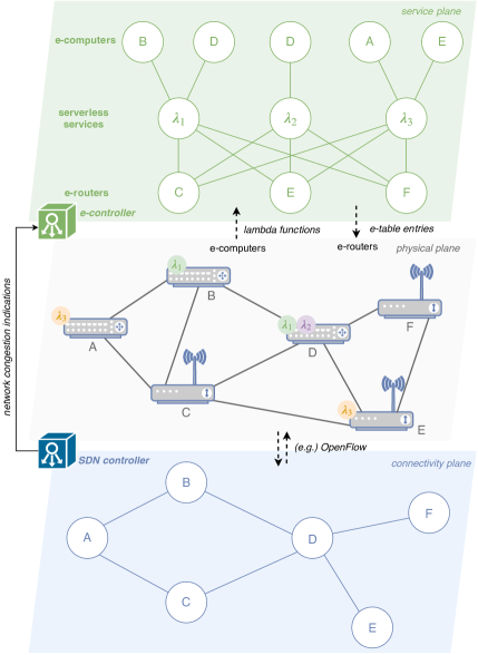
Figure 2: System model example, showing the service plane (as perceived by the e-controller) and the connectivity plane (as perceived by the SDN controller).

The complete system model is illustrated by means of the example in Fig. 2, also showing: (iii) the SDN controller, which has responsibility for maintaining connectivity in the network and provides up-to-date topology and network congestion information; (iv) the edge controller (e-controller), which discovers the capabilities of the e-computers in the domain and configures accordingly the e-routers so that they can set up and maintain their e-router forwarding tables (e-tables).

Therefore, to make the forwarding process of e-routers reactive to the fast changing conditions in an edge system we introduce the concept of weight, which is assigned by e-router $s$ to every destination e-computer $d$ and lambda function $i$, and denoted as $w^{s}_{i,d}$ in the following. Such weight is a measure of the cost to execute the associated lambda on the target e-computer from the point of view of a given e-router: the lower the cost, the more desirable the destination. Weights are adapted over time by every e-router independently, so that this process is lightweight and may follow closely the load/application variations on a time scale that is intermediate between the add/removal of entries in the e-tables and the per-lambda destination selection.

Our definition of e-tables in the e-routers basically establishes an overlay model of an edge domain for serverless computing, as illustrated in the top part of Fig. 2. At a steady state, the overlay looks the same to all e-routers, but the weights associated to the same lambda and destination may be different on each e-router, since they depend on the connectivity of the e-routers to the respective e-computers and the past history of executions experienced. In this work we tackle the following research challenges: how to keep the weights updated in the e-tables over time and which destination to select for every incoming lambda request (Sec. IV) and how to achieve scalability as the size of e-tables increases (Sec. V).

Finally, we note that our solution gracefully fits into the ETSI MEC reference architecture, as shown in the supplementary material.

IV E-router algorithms

In this section we propose algorithms for the realization of an efficient execution of serverless functions in the architecture illustrated in Sec. III, separately for the two sub-problems of weight updating and destination selection described therein.

IV-A Weight updating

From Sec. III, the weight updating problem at e-router $s$ for lambda $i$ consists in deciding how to assign $w^{s}_{i,d}$ so that this value reflects a smaller cost incurred by a client if the function is executed by computer $d$ than that paid if it was executed by computer $d^{\prime}$, where $w^{s}_{i,d}<w^{s}_{i,d^{\prime}}$. It is clear that, from a design perspective, weight updating depends on the objective function that we wish to pursue. In principle, there are several goals that one may pursue when designing a system for edge computing: energy efficiency, IP traffic balancing, user application latency reduction. While all objective functions have some relevance in the big picture, we believe the latter, i.e., minimization of latency, will be one of the key drivers for edge computing adoption, and hence it is considered in this work as the chief performance goal to be achieved. In fact, we aim at setting $w^{s}_{i,d}$ equal to the expected latency incurred by e-router $s$ if forwarding lambda function $i$ to the e-computer $d$.

There are several components that contribute to such latency: (i) processing delayat the e-computer, both directly due to the execution of $\lambda_{i}$ itself and indirectly caused by other concurrent tasks; (ii) transfer delay, including the hop-by-hop transmission of data from the client to the e-router to the e-computer and back to the client, any transport protocol overhead, and queuing at all intermediate routers and switches; (iii) application queuing delay, which may happen if the e-computer has a pre-allocated number of workers per VM/container. Furthermore, we expect the components above to be highly variable over time and difficult to predict in most use cases of practical interest for IoT. Therefore, static manual configuration of weights based on off-line analysis is not a viable option. Instead, we consider a common smoothed average rule for weight updating.

Specifically, each e-router $i$ performs an independent update of the weight $w^{i}_{j,d}$ associated to lambda $\lambda_{j}$ directed to destination $d$:

$$w^{i}_{j,d}(t^{+})=\begin{cases}\infty&\text{if net cong}\\ \alpha\cdot w^{i}_{j,d}(t^{-})+(1-\alpha)\cdot\delta_{j,d}(t^{+})&\text{otherwise}\end{cases}$$ (1)

where $\delta_{j,d}(t^{+})$ is the latency measured at current time $t^{+}$ for $\lambda_{j}$ executed by e-computer $d$, $w^{i}_{j,d}(t^{-})$ is the weight’s previous value (if no such value is available then it is $w^{i}_{j,d}(t^{+})=\delta_{j,d}(t^{+})$), $\alpha$ is a smoothing factor, and the condition “if net cong” (= if there is temporary network congestion along the path from e-router $i$ to e-computer $d$) is indicated by the e-controller to the e-router $i$ as needed.

Such congestion cases may be detected by the SDN controller using any existing network monitoring mechanism and conveyed to the e-controller, which will therefore proactively disable the corresponding entry on the e-routers to avoid undesirable delays and exacerbating congestion further (first condition in Eq. (1)). As the congestion situation is resolved, either due to decreased demands or because of a reconfiguration of the network paths, the weight will be restored to the last value it had before congestion. On the other hand, under normal network conditions, the second condition in Eq. (1) will continuously keep the weight aligned with the average overall latency, without distinguishing on whether it is due to processing or transfer. This is consistent with the objective of minimizing latency as a user-centric, rather than network- or operator-centric, metric.

IV-B Destination selection

The destination selection problem consists in finding at e-router $s$ the best e-computer $\bar{d}$ where an incoming lambda $i$ request should be forwarded, among the possible destinations $d\in\mathcal{D}_{i}$, each assigned a weight $w^{s}_{i,d}$. Since the weight, according to the update procedure in Sec. IV-A, is a running estimate of the latency, a trivial solution to the destination selection problem could be to always select the destination with the smallest weight. However, the same algorithm is used by all the e-routers in the edge computing domain and, as the reader may recall from Sec. III, by design the e-routers do not communicate with one another (either directly or through the e-controller), to keep the process lightweight and scalable to a high number of e-routers. Therefore, we argue that such a simplistic approach could, in principle, be inefficient because of undesirable herd effects, which are well known in the literature of scheduling in distributed systems [31]. Briefly, if all e-routers agree that e-computer $x$ is the best one to serve a given lambda $i$, then all will send incoming requests to it, thus overloading it, which eventually will result in performance degradation, which will make all e-routers move together towards the former second-best e-computer $y$, which will then become overloaded, and so on. To capture the need for a compromise between selfish minimization of delay and fair utilisation of resources, we redefine the well-established notion of proportional fairness (e.g., [19]) as follows: a destination selection algorithm is fair if any destination is selected a number of times that is inversely proportional to its weight. In other words, this means that a “proportional fair” destination selection algorithm tends to select (proportionally) more frequently a destination with a lower weight, i.e., latency estimation. This notion also embeds an implicit assumption of load balancing if the dominant effect on latency is the processing time.

In the following we propose three algorithms that exhibit an incremental amount of proportional fairness, ranging from none to short- and long-term proportional fairness. Their performance in realistic complex scenarios will be evaluated by means of emulation experiments in Sec. VI. In the remainder of this section we assume, for ease of notation, that only the destinations with weight $<\infty$ are considered.

IV-B1 Least-impedance

The least-impedance (LI) policy is to send the lambda request to $\bar{d}$, where $\bar{d}=\arg\min_{j}w_{j}$.

Quite clearly, this policy is a limit case where there is no proportional fairness at all: LI is an extremely simple greedy approach which does not require any state to be maintained at the e-router. On the other hand, it may suffer from the herd effect mentioned above.

IV-B2 Random-proportional

The random-proportional (RP) policy is to send the lambda request to $d$ with probability $1/w_{d}$.

It is straightforward to see that RP enjoys the property of long-term proportional fairness: over a sufficiently large observation interval the ratio between the number of lambda requests served by any two e-computers $i$ and $j$ is $N_{i}/N_{j}=w_{j}/w_{i}$. However, in the short-term, fairness is not provided: due to the probabilistic nature of this policy, there is no mechanism preventing any destination (or sub-set of destinations) to be selected repeatedly for an arbitrary number of times, thus making RP arbitrarily unfair over any finite time horizon.

IV-B3 Round-robin

The round-robin (RR) algorithm is inspired from a high-level discussion in [12] and combines together the proportional nature of RP with the greediness of LI. With RR we maintain an active list of destinations $\mathcal{A}=\{w_{j}|w_{j}\leq 2\cdot\min_{h}w_{h}\}$. For each destination $j\in\mathcal{A}$ we keep a deficit counter $\Delta_{j}$ initially set to $0$. The policy is then to send the lambda request to $d=\arg\min_{j}\Delta_{j}$ and at the same time increase $\Delta_{d}$ by $w_{d}$. Once a destination goes out of the active list, it is re-admitted for a single “probe” after an initial back off time, doubled every time the probe request fails to meet the active list admission criterion; when the active set is updated we decrease all $\Delta_{j}$ by $\min_{h}\Delta_{h}$. We note that, as a new destination is added, a trivial implementation following from the algorithm definition would have $\mathcal{O}(n)$ time complexity since all destinations in $\mathcal{A}$ need have their deficit counter updated. However, a simple data structure that avoids such linear update can be adopted: the active destination deficit counters can be stored in a list sorted by increasing deficit counters, where only the differences with the previous elements are kept. For instance, if the deficit counters are $\{4,6,7,7\}$ the data structure will hold $\{4,2,1,0\}$; since the front element of the list is always the minimum, the update can be done in $\mathcal{O}(1)$ by simply resetting this value.

initialization: $\mathcal{A}=\mathcal{P}=\emptyset$, $\forall j:w_{j}=e_{j}=0,b_{j}=b_{\min}$ function leastImpedance(): return $\arg\min_{j}\left\{w_{j}\right\}$ function randomProportional(): return random $d$ with probability $1/w_{d}$ function roundRobin(): select random $d\in\left\{j|e_{j}>now()\land j\notin\mathcal{P}\right\}$ if $\exists d$: $\mathcal{P}=\mathcal{P}\cup\{d\}$ else: $d=\arg\min_{j}\left\{\Delta_{j}|j\in\mathcal{A}\right\}$ $\Delta_{d}=\Delta_{d}+w_{d}$ return $d$ function onReceiveResponse($\delta,d$): ($\delta$ is the latency measured for the response from $d$) if leastImpedance $\lor$ randomProportional: $w_{d}=\alpha\cdot w_{d}+(1-\alpha)\cdot\delta$ else: /* roundRobin */ if $d\in\mathcal{P}$: $\mathcal{P}=\mathcal{P}\setminus\{d\}$ if $\delta\leq 2\cdot\min_{j}\left\{w_{j}|j\in\mathcal{A}\right\}$: $\forall j\in\mathcal{A}:\Delta_{j}=\Delta_{j}-\min_{j}\{\Delta_{j}\}$ $\mathcal{A}=\mathcal{A}\cup\{d\}$ $b_{d}=b_{\min},\Delta_{d}=w_{d}=\delta$ else: $b_{d}=2\cdot b_{d},e_{d}=now()+b_{d}$ else: $w_{d}=\alpha\cdot w_{d}+(1-\alpha)\cdot\delta$ if $w_{d}>2\cdot\min_{j}\left\{w_{j}|j\in\mathcal{A}\right\}$: $\mathcal{A}=\mathcal{A}\setminus\{d\}$

Figure 3: Pseudo-code of the algorithms in Sec. IV.

The algorithms presented so far in natural language are also described with the pseudo-code in Fig. 3 (corner cases not addressed for simplicity, we refer the interested reader to the real implementation, available as open source for full details), where $b_{j}$ is the relative backoff time before a destination is probed for its inclusion in the active list (starting with minimum value $b_{\min}$) and $e_{j}$ is the absolute time when it will be considered for inclusion in the set $\mathcal{P}$ of probed destinations. Note that least-impedance and random-proportional only use $w_{j}$ state variables.

In the following we show that RR achieves both short-term and long-term proportional fairness. To this aim, we introduce a more formal definition of the algorithm. Let $\mathcal{A}$ be the set of active destinations, each with a deficit counter $\Delta_{i}$ initialized to $0$. At time $n$, select destination $x=\arg\min_{i}\{\Delta_{i}\}$, breaking ties arbitrarily; then, update the deficit counter of the destination selected as follows: $\Delta_{x}=\Delta_{x}+\tilde{\delta_{x}}$, where $\tilde{\delta_{x}}$ is an estimate of the time required for the lambda function requested to complete if forwarded to edge computer $x$. We denote as $\delta_{x}$ the actual completion time, but this cannot be known at the time the forwarding decision is taken. When a new edge computer $y$ is added to $\mathcal{A}$ it is assigned $\Delta_{y}=0$ and all the other deficit counters are updated as follows:

$$\Delta^{\min}=\min_{i\in\mathcal{A}\setminus y}\left\{\Delta_{i}\right\}$$ (2)

$$\forall i\in\mathcal{A}\setminus y:\Delta_{i}=\Delta_{i}-\Delta^{\min}$$ (3)

After each update $\exists i\in\mathcal{A}|\Delta_{i}=0$.

Lemma 1.

The difference between any two deficit counters is bounded by a finite constant equal to the maximum completion time estimate ($\tilde{\delta}^{\max}$), i.e.:

$$\max_{i,j}\left\{\Delta_{i}-\Delta_{j}\right\}\leq\tilde{\delta}^{\max}$$ (4)

Proof.

The statement can be proved by contradiction. Assume:

$$\exists i,j|\Delta_{i}(n)-\Delta_{j}(n)=\tilde{\delta}^{\max}+\epsilon$$ (5)

Without loss of generality, we can assume that $i$ was the destination selected at time $n-1$ (it this was not the case, then one can substitute $n-1$ in the following with the last time $i$ was selected; meanwhile we can assume that $j$ was never selected otherwise its deficit counter would have increased, which would have reduced the gap between deficit counters). In this case, it is:

$$\Delta_{i}(n-1)=\Delta_{j}(n-1)=\Delta_{j}(n)$$ (6)

Putting together Eq. (5) and Eq. (6) we obtain:

$$\Delta_{i}(n) =\Delta_{j}(n)+\tilde{\delta}^{\max}+\epsilon=$$ (7)

$$=\Delta_{i}(n-1)+\tilde{\delta}^{\max}+\epsilon$$ (8)

From which it is:

$$\tilde{\delta}_{i}=\tilde{\delta}^{\max}+\epsilon$$ (9)

Which is impossible for any $\epsilon>0$ by definition of $\tilde{\delta}^{\max}$. ∎

In the following we assume for simplicity that the completion time estimates are constant over time, i.e. it is $\tilde{\delta}_{i}(n)=\delta_{i}$ for any destination $i$. Furthermore, we define $s_{i}(n)$ as the number of times the destination $i$ was selected by the forwarding algorithm since $n=0$.

Lemma 2 (short-term fairness).

For any two destinations $i,j$ at any time $n$ the difference between their number of services weighted by the respective completion time is bounded by the maximum completion time $\delta^{\max}=\max_{i}\{\delta_{i}\}$:

$$\forall i,j\in\mathcal{A}:s_{i}(n)\delta_{i}-s_{j}(n)\delta_{j}\leq\delta^{\max}$$ (10)

Proof.

To prove the statement let us consider the update process of both $s_{i}(n)$ and $\Delta_{i}(n)$:

$$s_{i}(n)=s_{i}(n-1)+\begin{cases}1&\text{if }i=\arg\min_{j}\left\{\Delta_{j}(n-1)\right\}\\ 0&\text{otherwise}\end{cases}$$ (11)

$$\Delta_{i}(n)=\Delta_{i}(n-1)+\begin{cases}\delta_{i}&\text{if }i=\arg\min_{j}\left\{\Delta_{j}(n-1)\right\}\\ 0&\text{otherwise}\end{cases}$$ (12)

From Eq. (5) and Eq. (6) it follows that:

$$\Delta_{i}(n)=s_{i}(n)\delta_{i}$$ (13)

which proves the statement with Lemma 1. ∎

TABLE I: Visual forwarding example used in Lemma 3 with three destinations with $\delta_{1}=2$, $\delta_{2}=3$, $\delta_{3}=4$.

$\Delta_{1}$	0	2			4		6		8		10			12	$s_{1}=6$
$\Delta_{2}$	0		3			6				9			12		$s_{2}=4$
$\Delta_{3}$	0			4				8				12			$s_{3}=3$
time	0	1	2	3	4	5	6	7	8	9	10	11	12	13

Lemma 3 (long-term fairness).

Over a long enough time horizon the number of services of any destination $i$ is inversely proportional to its completion time $\delta_{i}$, i.e.:

$$\exists i,j\in\mathcal{A},n>0|\frac{s_{i}(n)}{s_{j}(n)}=\frac{\delta_{j}}{\delta_{i}}$$ (14)

Proof.

Let us start with the assumption that $\delta_{i}\in\mathbb{N}$. In this case, using the visual example in Table I, it is easy to see that there is a time $n^{*}$ where $\Delta_{i}=\Delta_{j}$ for any $i,j$, which can be computed as:

$$n^{*}=\sum_{i}\frac{T}{\delta_{i}}$$ (15)

where $T=lcm_{i}\{\delta_{i}\}$, which gives:

$$s_{i}(n^{*})=\frac{T}{\delta_{i}}$$ (16)

from which the lemma follows. The statement can be easily extended to the case of $\delta_{i}\in\mathbb{Q}$ as follows. Find $D$ as the LCM of the denominators of $\delta_{i}$, then set $\delta^{\prime}_{i}=D/den(\delta_{i})$. We now have new $\delta^{\prime}_{i}$ values that are in $\mathbb{N}$ by construction and the same method as above can be used. ∎

V Scalability extension

In this section we study the scalability of our proposed architecture in terms of the number of serverless functions offered by the e-computers.

In Sec. III we foresee a flat overlay where each e-router is notified of the existence of any lambda function offered by an e-computer by the e-controller, including a means to reach it (such a Uniform Resource Identifier (URI) or a service end-point). This means that every e-router is required to keep one entry in its e-table for every lambda function in the network (say $\Lambda$). In Sec. IV we have put forward algorithms that are simple and efficient to both keep the entry’s weight updated and select the destination for any incoming lambda, yet performance may suffer as $\Lambda$ becomes very big, especially if the e-routers are low-end devices such as Single-Board Computers.

To verify this claim, we have carried out the following experiment on a Raspberry Pi 3 Model B (RPi3), which is “representative of a broad family of smart devices and appliances” [24], where we have installed an e-router and added an artificial number of entries in its e-table. Then, we have started a number of clients repeatedly asking for a lambda function to be executed. In particular, we have used 10 clients, as the minimum number for which the computation resources of the RPi3 were saturated. The e-routers have been modified for the purpose of the experiment so that, instead of actually forwarding the lambda request to an e-computer and reporting back the result to the client, it just replied with a successful but empty response for any lambda. All other phases, such as weight computation, destination selection, and any housekeeping operations, were performed exactly as in a real environment. This experiment provides us with an upper bound of the number of lambda functions that can be processed concurrently by an e-router on a RPi3 as the e-table size increases. We have run 10 experiments but the variance was negligible compared to the mean values, thus we report only the latter in the plot; similarly, we report only the results with RR as the destination selection algorithm, because the other algorithms gave similar results leading to the same conclusions.

Figure 4: RPi3 e-router processing rate vs. num. forwarding table entries.

In Fig. 4 we show the normalized processing rate, which decreases steadily as the e-table increases at steps of 1,000 entries at a time, showing an asymptotic behavior with very big tables that is consistent with a $\mathcal{O}(\log(\Lambda))$ average time complexity, which can be inferred a priori since the algorithms involved require a look-up in a sorted data structure to both retrieve the weight and select the next destination. The results confirm the intuition that the size of the e-table may become a choke point in a production environment as the number of lambda functions increases to realistic values, at least with devices with limited processing capabilities.

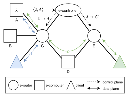
Figure 5: Extension of the proposed architecture to improve scalability.

To enhance scalability while keeping the same architecture and functions of the e-routers and e-computers, we propose the following optional extension of the e-controller. Recall that the e-controller is notified of the lifecycle of lambda functions on computers, i.e., start-up and tear-down of their serverless executors. Rather than announcing a new lambda function from the e-computer to all the e-routers, the e-controller can announce that to only some e-routers, while the others are notified that the lambda can be executed by one of the latter. Let us explain this concept with the example in Fig. 5, which shows what happens as the e-computer A announces $\lambda$ to the e-controller. The latter announces to C that $\lambda$ can be executed by A, but it tells E that $\lambda$ can be executed by C. Obviously, with a single instance of $\lambda$ there is no advantage since both e-routers will have exactly one entry in their e-table. However, imagine that a new lambda is then started on e-computer B and the e-controller does the same as before: in this case, the e-table of C grows by one entry, but the e-table of E remains the same because it already knows that it is possible to execute $\lambda$ via C. In the example in Fig. 5 we also show the data plane flows associated to two clients, connecting to the edge computing domain through C and E, respectively. Therefore, this hierarchical overlay allows the e-tables to grow less than linearly with the number of lambda services. In the supplementary material we also explain how to deal with forwarding loops, which may arise in more complex network topologies. The solution is to distinguish between final and intermediate destinations when advertising e-table entries, the former being preferred over the latter when forwarding.

Such a two-tier overlay could be easily extended to the case of $n$ tiers, however we do not consider this case because we believe that just one indirection level is sufficient to achieve scalability while keeping the protocol and processing overhead to a bare minimum. In Sec. V-A below we propose an algorithm that can be used by the e-controller to determine which entries to announce to the e-routers, based on external knowledge of the network topology.

V-A An e-table distribution algorithm

We now propose a practical algorithm that can be used by the e-controller to realize the hierarchical overlay described above. First, we note that it is a responsibility of the e-controller alone to announce entries in such a way that clients connecting from any e-router can always consume all the available services. This basic functional requirement translates into: for every lambda, any e-router must have in its e-table either a final destination to an e-computer offering that lambda, or intermediate destinations which, in turn, have at least one such final destination. Otherwise, a lambda request might get “stuck” at an e-router. Second, we argue that the e-controller should use network topology information to take its decisions: (i) such information is readily available from the SDN controller and it is likely to change slowly over time, at least as far as the e-routers and e-computers are concerned; (ii) disregarding connectivity may lead to inefficient allocation of e-table entries, e.g., a final entry for an e-computer may be installed on an e-router whose network cost is very high, thus forcing all other e-routers going through that to consume much more network resources than needed, in addition to adding significant delay to the data plane.

Therefore, in the following we assume that the e-controller is aware of the distance matrix $\{d_{ij}\}$ between any two edge nodes $i$ (source) and $j$ (destination), which in a real environment can be acquired through the SDN controller. We further simplify the problem by assuming that the e-controller identifies for each e-computer a home e-router. For all the lambdas of an e-computer, the home e-router is always advertised as final to itself and as intermediate to every other e-router. We believe this approach is very practical since it allows the e-controller to pre-compute for all possible e-computers their respective home e-routers, saved in a dedicated look-up table used whenever a new lambda appears. This is very useful since the rate at which the topology changes is expected to be much lower than that of lambda functions’ lifecycle changes, which may occur based on some autoscaling feature available in the edge computing domain, as mentioned earlier.

Under this assumption, the operation of the e-controller becomes straightforward:

• as a new lambda function is announced from e-computer $c$: look up $c$’s home router $\bar{r}$; announce a final destination entry towards $c$ to $\bar{r}$; announce an intermediate destination towards $\bar{r}$ to any $r\neq\bar{r}$, unless already announced;

• as a lambda function is torn down by e-computer $c$: look up $c$’s home router $\bar{r}$; remove the final destination entry towards $c$ from $\bar{r}$; remove an intermediate destination towards $\bar{r}$ from any $r\neq\bar{r}$, unless there is at least one other final destination towards $c^{\prime}\neq c$ in $\bar{r}$ for the same lambda.

Thus, the only remaining issue is how to select the home e-router of an e-computer. To this aim, we propose to pursue one of the following two objectives: min-max, where the choice of the home e-router minimizes the maximum cost that has to be paid by a client accessing from any e-router to reach the home e-router and from it the final destination e-computer; or, min-avg, where we strive to minimize the same cost paid by clients accessing from all e-routers, on average. In any of the two policies we break ties based on the result that would be obtained if using the other policy (further ties are broken arbitrarily). Both policies are captured by the following objective (we use the sum instead of the average since the number of e-routers is a constant):

$$\min_{i\in\mathcal{R}}\left\{\Omega\max_{j\in\mathcal{R}}\left(d_{ic}+d_{ij}\right)+\omega\sum_{i\in\mathcal{R}}\left(d_{ic}+d_{ij}\right)\right\}=$$

$$\min_{i\in\mathcal{R}}\left\{\Omega\left(d_{ic}+\max_{j\in\mathcal{R}d_{ij}}\right)+\omega\left(\left|\mathcal{R}\right|d_{ic}+\sum_{i\in\mathcal{R}}d_{ij}\right)\right\},$$ (17)

where $\mathcal{R}$ is the set of all e-routers, and $\Omega$, $\omega$ are constant factors that can be used to shift from min-max to min-avg: if $\Omega\gg\omega$ then the policy is min-max, otherwise if $\Omega\ll\omega$ it is min-avg, where the ratio between the two must be large enough that the maximum always overpowers the average, e.g., $\Omega/\omega>2\left|\mathcal{R}\right|D$, where $D$ is the connectivity graph’s diameter.

Regardless of the objective function, the search of the home e-router of a single e-computer is $\mathcal{O}(|\mathcal{R}|^{2})$, hence the overall process to find the home e-routers for all e-computers if $\mathcal{O}(|\mathcal{R}|^{2}|\mathcal{C}|)$, if $\mathcal{C}$ is the set of the e-computers. The algorithm must be executed only by the e-controller and only upon changes of the connectivity of edge nodes or the set of lambda functions offered by them. We believe that in many use cases of practical interest both these events will be much less frequent than lambda function execution, i.e., order of magnitude of minutes and above for the former vs. seconds and below for the latter. A more optimized algorithm, tailored to the specific deployment, can be devised and implemented instead on the e-controller, if needed, with no impact at all on the other system components.

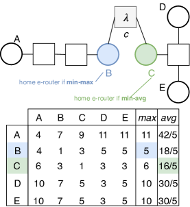
Figure 6: Determining the home e-router in an example topology: min-max vs. min-avg.

In Fig. 6 we show an example of determining the home e-router of an e-computer offering $\lambda$. We assume that the cost of all hops is equal to 1 and that the distance matrix is symmetric (note that this is just for the sake of the example: the algorithm in this section supports asymmetric paths). On the right we report a matrix where element $x_{ij}$ is the sum of the cost to go from e-router $i$ to the e-router $j$ and from there to the e-computer $c$, i.e. $d_{ic}+d_{ij}$ as in Eq. (V-A). In the example, B is selected as the home e-router if min-max is used because the maximum path D—B—$c$ (or E—B—$c$, both with cost 5) is smaller than the maximum path that would exist if any other e-router is selected as home, including C for which the maximum path would be A—C—$c$ (cost 6). However the e-router C is more central to the network topology, as reflected by the smaller average distance, and it is therefore selected as home of $c$ with min-avg.

We note that the proposed approach may lead, in general, to sub-optimal routing of lambda requests/responses. For instance, with reference to Fig. 6 with a min-avg policy, the path followed by a lambda request from A in terms of “forwarding hops” is A—C—$c$, but in “networking hops” this requires A—B—$c$—C—$c$, which is clearly inefficient since, in principle, the request could have stopped at $c$ the first time it got there. However, we believe the ends justify the means: by tolerating sub-optimal transfer of lambda requests, we can keep the design of the solution, based on the concept of “home e-router”, simple and efficient. Anyway, in many cases of practical interest the performance degradation due to the detours could be negligible, as shown by the results of the experiments in Sec. VI-D obtained using a realistic network map.

V-B Analysis

In qualitative terms, the hierarchical overlay proposed above trades off response delay (increased because of one additional hop from the client to the e-computer) for computational complexity in the e-routers (decreased by having smaller e-tables, which occupy less memory and yield a faster look-up). In this section we perform a quantitative analysis of these two aspects in simplifying conditions, which will be complemented in Sec. VI by emulation experiments in more realistic environments.

We start with the computational complexity. The actual size of an e-table will, by necessity, depend on the relative distance of the e-routers and the e-computers offering each lambda, and it cannot be predicted a priori. Rather, it is easy to forge limit cases where the maximum size of the e-table is not reduced at all by the hierarchical scheme proposed. Consider for instance a network where all e-computers have to pass through an e-router, acting as a sort of default gateway, which then connects to all the other e-routers in the edge domain: in this case the e-table of the “gateway” will contain all the lambda in the network (as it would if a flat overlay was used), while all the others would contain a single entry pointing to the “gateway” itself. Such degenerate cases are of limited interest, since they would call for ad hoc solution anyway.

Thus, we argue that a case where the e-routers and e-computers are distributed rather uniformly over the edge domain, in a topology sense, is much more realistic, especially since we consider IoT environments whose nature is often distributed over large coverage areas. Under these reasonable assumptions, every e-router is bound to have approximately the same chances as any other to be selected as the home e-router for a given e-computer/lambda. Thus, reusing the same notation as above, an approximation of the average number of entries in an e-table for every $\lambda$ served by $\mathcal{C}_{\lambda}$ e-computers is:

$$n_{entries}\approx\begin{cases}|\mathcal{C}_{\lambda}|&\text{if }|\mathcal{C}_{\lambda}|\ll|\mathcal{R}|\\ |\mathcal{R}|+\frac{|\mathcal{C}_{\lambda}|}{\mathcal{R}}&\text{if }|\mathcal{C}_{\lambda}|\gg|\mathcal{R}|\\ \end{cases}.$$ (18)

An explanation of Eq. (18) is the following: when the number of e-computers serving a given lambda is small, compared to the number of e-routers, then there are little or no advantages in using a hierarchical overlay, since in a uniformly distributed topology the chance of the few lambdas “colliding” in the same e-router are small anyway; however, if this is the case, then it is not necessary to use a hierarchical overlay, because its only motivation is to limit the size of e-tables as the number of lambda functions increases significantly. In this case, i.e., the bottom branch of Eq. (18), (almost) all the e-routers will have at least one e-computer offering a given lambda, hence every e-router will have to have one entry for each $r\in\mathcal{R}$, in addition to the lambda functions for which it is a home router, which will split evenly among all the e-routers in the network, hence amounting to $\frac{|\mathcal{C}_{\lambda}|}{\mathcal{R}}$. In a large edge computing domain, where scalability must be considered as as potential issue, we definitely expect to have many e-routers ($|\mathcal{R}|$ is big), hence a two-tier overlay is sufficient to keep the pace at which e-table sizes grow much slower than the lambda increase rate.

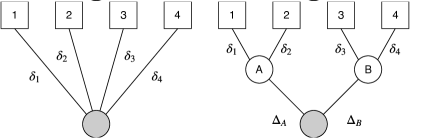
Figure 7: Example with four e-computers to illustrate the effect of using a hierarchical overlay on the average delay.

We now focus on the increased response delay. To this purpose, let us consider the example in Fig. 7, showing on the left-hand side an e-router having on its e-table four final destinations, numbered from 1 to 4. Under the notion of proportional fairness introduced in Sec. IV-B, assuming for simplicity that the delays remain constant over time and over a sufficiently long period, every destination $i$ will be selected more frequently proportionally to the inverse of its delay $\delta_{i}$. This means that the average delay experienced, in general with $n$ destinations, is:

$$E[\delta]=\frac{\sum_{i=1}^{n}\delta_{i}\frac{1}{\delta_{i}}}{\sum_{i=1}^{n}\frac{1}{\delta_{i}}}=\frac{n}{\sum_{i=1}^{n}\frac{1}{\delta_{i}}},$$ (19)

which is the harmonic mean of the delays, which in the example is:

$$E[\delta]=4\frac{\prod_{i=1}^{4}\delta_{i}}{\sum_{i=1}^{4}\frac{1}{\delta_{i}}\prod_{i=1}^{4}\delta_{i}}$$ (20)

Let us now see what happens if another level of forwarding is added, by introducing e-routers A (home to e-computers 1 and 2) and B (home to e-computers 3 and 4), assuming that reaching A (B) incurs an additional delay $\Delta_{A}$ ($\Delta_{B}$). By substitution and simple algebraic simplification, we obtain:

$$E[\delta]=4\frac{\prod_{i=1}^{4}\delta_{i}+G_{A}^{2}\Delta_{B}A_{B}+G_{B}^{2}\Delta_{A}A_{A}+\Delta_{A}\Delta_{B}A_{A}A_{B}}{\sum_{i=1}^{4}\frac{1}{\delta_{i}}\prod_{i=1}^{4}\delta_{i}+2(\Delta_{A}+\Delta_{B})A_{A}A_{B}},$$ (21)

where $G_{A}=\sqrt{\delta_{1}\delta_{2}}$ is the geometric mean of the delays incurred when reaching the lambda through A and $A_{A}=\frac{\delta_{1}+\delta_{2}}{2}$ is their arithmetic mean (and likewise for $G_{B}$ and $A_{B}$). We note two properties from Eq. (21). Firstly, if the additional forwarding delays $\Delta_{x}$ are small compared to the processing delays $\delta_{y}$ then Eq. (21) becomes exactly Eq. (20), because all the addends after the first in both the numerator and the denominator become negligible with respect to the first component. We expect this assumption to be true in many cases of practical interest, since it basically means that the latency due to transferring the input and output of a lambda is much smaller than the time it takes an e-computer to process it. Secondly, even when this is not applicable, it is clear from Eq. (21) that the variations to the average delay introduced by the $\Delta_{x}$ are smooth, i.e., they do not change abruptly the behavior dictated by the $\delta_{y}$ values.

VI Performance evaluation

In this section we provide a comprehensive experimental performance analysis of the contributions proposed in this work by means of three different scenarios, designed to validate in particular one aspect of the overall solution proposed. Specifically, the decentralized architecture (Sec. III) is studied in a scenario with a grid network topology (Sec. VI-B), also illustrating the behavior of the destination selection algorithms in Sec. IV-B; the latter are also subject to analysis in the second scenario (Sec. VI-C), which however focuses on showing the benefits of explicit congestion notification as proposed in Sec. IV-A. The results will show that our proposed framework, with multiple decentralized serverless platforms, can achieve almost the same performance as a hypothetical distributed system running at the edge with same aggregate capacity. Finally, the e-router scalability described in Sec. V is assessed in a large-scale realistic scenario (Sec. VI-D), showing a reduction of the size of e-tables of about 20%, compared to a flat overlay, without a noticeable degradation in terms of the delay (which in some cases is even decreased, as explained later). Further results are provided as supplementary material.

VI-A Environment and methodology

We have used our own performance evaluation framework with real applications running in Linux namespaces interconnected via a network emulated with Mininet. The interested reader may find full details in [10], which also describes the details of the implementation of the e-routers and e-controller. As executors we have used both OpenWhisk (as in [4]) running in Docker containers and emulated e-computers, which provide responses to lambda requests based on the simulation of processing of tasks in a multi-processing system, also illustrated in [10].

The experiments have been run on a Linux Intel Xeon dual socket workstation that was not used by any concurrent demanding application. The smoothing factor $\alpha$ in Eq. (1) was set to 0.95 based on preliminary calibration experiments whose results are not reported here. In the plots we report confidence intervals (unless negligible) with a 95% confidence level, computed over 20-30 independent replications of each experiment, depending on the scenario.

VI-B Grid scenario

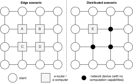
Figure 8: Grid scenario network topology (Sec. VI-B).

We begin our analysis with a scenario in a grid topology, shown in Fig. 8 (left part), with 100 Mb/s bandwidth / 100 $\mu$s latency links. As in [12], the executors are in the middle of the grid, while the exterior nodes act as clients; every host with an executor also hosts an e-computer. We compare our proposed solution (called Edge/dynamic, using RR as a destination algorithm) with an alternative with no e-routers, where clients simply request execution of lambda functions from the closest executor (called Edge/static). We also run experiments in a slightly different setup, with a single more powerful executor having computational capabilities equal to the sum of all the executors in the other setup. Such an environment, illustrated in the right part of Fig. 8 and called Distributed, is representative of a traditional serverless deployment (like in the left part of Fig. 1). The results obtained with Distributed, therefore, are intended only as a reference, not in comparison to those in Edge environments.

In the first batch of results, the executors use OpenWhisk: nodes A–D are reserved two CPU cores each, while node E is given eight. We have implemented two toy lambda functions, which stress respectively I/O and CPU. Every client requests their execution with an Interrupted Poisson Process (IPP) pattern with busy / idle periods equal to 2 s / 6 s, on average; within a busy period, the client triggers 3 lambda functions per second; lambda functions that would extend the busy period because of accumulated delay are dropped, instead. Clients are independent of one another. We ran experiments with a variable number of clients.

Figure 9: Grid scenario (with OpenWhisk executors): CDF of delay with I/O- and CPU-intensive tasks, with 24 clients.

We first evaluate the delay, defined as the time between when the client is scheduled a lambda function and the time when it receives a response. In Fig. 9 we show the CDF of the delay with 24 clients, corresponding to a moderate overall load. With both types of lambda functions, using e-routers is beneficial in terms of high quantiles of the delay: a static allocation provides similar (or better) performance in those times when there are fewer requests to a given executor, but when the load increases it is unable to balance in the pool of resources available. The delay with Distributed is smaller than with Edge: this confirms the intuition that serverless in a cloud-like environment is easiest with mainstream technologies, though not always possible because of deployment constraints.

Figure 10: Grid scenario (with OpenWhisk executors): Lambda loss ratio with CPU-intensive tasks, with 24 and 36 clients.

In Fig. 10 we show the lambda loss ratio, defined as the ratio of lambda function calls that the client refrains from executing to avoid overrunning the active periods over the total scheduled. We report only the results with CPU-intensive tasks (those with I/O-intensive tasks are similar and omitted for lack of space), with 24 and 36 clients. As can be seen, with both loads a static allocation exhibits poor performance, with most clients experiencing a non-negligible loss. It is interesting to note that with 24 clients the Edge/dynamic and Distributed curves cross a little above 80% of clients: while there are more clients with non-negligible loss in the former, the clients experiencing some loss with Distributed have a higher loss than with Edge/dynamic. This is an effect of the fairness property of the RR algorithm illustrated in Sec. IV-B, which is confirmed with 36 clients: Edge/dynamic is the only curve that does not rise steeply as the fraction of clients in the $x$-axis increases.

Figure 11: Grid scenario (with emulated e-computers): 95th percentile of delay vs. number of clients.

In the following, we report results obtained by substituting the OpenWhisk servers with emulated e-computers, which allowed us to analyze the case with heterogeneous CPUs. In fact, we set the (simulated) speed of the CPU of executors A/B/C/D respectively as 1,000/2,000/3,000/4,000 MIPS, whereas E in the Distributed case has the sum of the speed of A–D, i.e., 10,000 MIPS. We increase the number of clients from 1 to 12; results with all the algorithms in Sec. IV-B are reported. In Fig. 11 we show the 95th percentile of delay as the number of clients increases. As expected, the Distributed curve lies below all the others. Furthermore, we note that Edge/LI performs very bad even at low loads: this is because of the “herd” effect, which makes hot spots the executors with fastest CPU. A static allocation performs worse than Edge/RR and Edge/RP, except at very low loads. Finally, Edge/RR exhibits a smaller 95th percentile of delay than Edge/RP, but only until the system becomes overloaded (i.e., with 8 clients or less): after that, the performance of RP is comparable or better than that of RR.

Figure 12: Grid scenario (with emulated e-computers): Difference between the maximum and minimum lambda loss ratio vs. number of clients.

In Fig. 12, we complement the results above with a measure of the fairness, as the difference between the maximum and minimum lambda loss ratio among all the clients. The behavior of Edge/LI is extremely erratic since it tries to always direct the clients to the fastest executors. On the other hand, Edge/RR and Edge/RP exhibit excellent fairness, thus confirming on the field the theoretical analysis in Sec. IV-B. As can be seen, Edge/Static shows non-negligible unfairness starting at 4 clients, despite the overall load is rather limited.

VI-C Network congestion scenario

Figure 13: Topology used in network congestion scenario (Sec. VI-C).

In this scenario we focus our attention on the mechanism of congestion notification from the SDN controller illustrated in Sec. IV-A. To this purpose, we set up the network illustrated in Fig. 13, with 10 Mb/s bandwidth / 2 ms latency links, and where we inject periodically background TCP traffic in the links between the middle node and the OpenWhisk executors, which are allocated 2-2-4 CPU cores. Only one link is interfered at a time. We use CPU-intensive tasks only. The clients, whose number increases from 5 to 30, are associated randomly to one of the three e-routers, and they issue two requests (10 kB each) per second, on average, uniformly distributed.

Figure 14: Network congestion scenario: 95th percentile of delay vs. number of clients, with all destination algorithms in Sec. IV-B, and with/without congestion detection in Eq. (1).

In Fig. 14 we report the 95th percentile of delay. As can be seen, without congestion notification, the 95th percentile of delay does not depend on the load: whenever there is congestion on a link, more than 5% of lambda requests are affected since the e-router on the congested link tries to execute them on executors after the path with background traffic. This is avoided by enabling the congestion notification mechanism. In this scenario, unlike that in Sec. VI-B, LI exhibits best performance, with RR being intermediate. This is because LI suffers most from executors having an uneven distribution of computational resources, which does not happen here. Overall, RR is found to be more flexible in different conditions than both RP and LI.

VI-D Large scale scenario

Figure 15: Large scale scenario (Sec. VI-D): Network map.

In this section we investigate the impact of using a two-tier overlay, as described in Sec. V, in a topology extracted from a real IoT network: Array of Things, simplified by collapsing nodes that are very close to one another. The resulting network map is illustrated in Fig. 15: it consists of 45 nodes with a diameter of 11 hops. All links have a 10 Mb/s capacity, with a 2 ms latency, emulating an urban Wireless Mesh Network (WMN). In this scenario we focus on the hierarchical forwarding scheme in Sec. V, hence we use emulated e-computers and clients issue lambda requests with a fixed input size (equal to 5000 bytes, corresponding to 8.3 ms processing time), so that the impact of network transfer on the lambda response latency shows significantly.

We have assumed that all edge nodes host exactly one e-computer offering the same lambda, whereas 10 e-routers are dropped at the beginning of every run in random edge nodes. We increased the number of clients from 30 to 120, and they also are dropped at random locations at the beginning of every experiment. During the experiment all clients continuously repeat the execution of the same lambda request, thus the total number of lambda executions is different for every run. We compare a flat overlay to a two-tier overlay with the min-max and min-avg policies defined in Sec. V-A. Furthermore, only for evaluation purpose, we add a third policy with a two-tier overlay, called random: select a random home e-router for every computer, thus emulating a topology-unaware algorithm to realize the overlay, such as if using a Distributed Hash Table (DHT), as proposed in [36]. The use of a two-tier overlay is found a posteriori to exhibit an average size of the e-tables equal to $8.4\pm 3.5$, while the size is always 45 with a flat overlay. The destination selection algorithm is always RR, since it has been shown above to provide the best performance compromise.

Figure 16: Large scale scenario: Mean and 99th percentile of delay.

In Fig. 16 we report the delay. As can be seen, both the mean and the 99th percentile show the same behavior, though more exacerbated in the latter, which is explained in the following. First, two-tier overlay (random) degrades the performance, even at low loads, and more so as the network becomes overloaded. This confirms our intuition in Sec. V that the network topology should be kept into account when determining the home e-routers in a two-tier overlay, otherwise a performance penalty must be paid because of the unnecessary long paths from the ingress e-router to the home e-router and then to the e-computer for every lambda request issued by a client. Second, a flat overlay entails slightly smaller delays at low loads: this is because it incurs less network transfer overhead, which is the dominating factors. However, as the number of clients increases, the e-computers become gradually more loaded, hence the processing time becomes the primary source of delay: in these conditions, a two-tier overlay, either min-max or min-avg, is always beneficial in terms of delay, with the latter (min-avg) yielding a 99th percentile of delay which is about 40% smaller than that with a flat overlay. The reason is that with a two-tier overlay lambda execution tends to reward proximity: remote e-computers are clustered and masked as a single destination by their respective home e-routers, hence probing is more lightweight and closer destinations are given a little more than their “fair” share

Figure 17: Large scale scenario: Average network load per lambda request.

Thus, a two-tier overlay is not only beneficial since it reduces the size of the e-tables, but it also yields smaller delays. This extremely positive result cannot be generalized to any possible environment: for instance, if the destinations closer to an e-router are overloaded for any reasons, then a flat overlay may utilize better resources that are far away but, in this case, preferable. However, we consider remarkable that a two-tier overlay, introduced as a necessity to reduce the size of e-tables for computational reasons at the calculated risk of increasing network overhead, does not in fact incur a penalty in terms of the latter in a realistic IoT network topology. To stress this point, we report in Fig. 17 a direct measure of the average cost, in terms of network resources, incurred by the execution of a single lambda. This measure is defined as the ratio of the overall number of bytes transmitted in the network by the total number of lambdas executed. As can be seen, the relative performance of the different approaches, in terms of this metric, is the same as in terms of the delay: the two-tier with random policy incurs the highest overhead by far, whereas the two-tier min-max and min-avg policies generally pay the smallest network cost.

VII Conclusions

In this paper we have proposed an architecture for the realization of serverless computing, which is of growing interest to IoT applications, in an edge network. The clients send lambda function requests to the e-routers, which forward them to the e-computers deemed to be most appropriate at the moment. The decision is taken based on weights local to every e-router, which is however notified by the SDN controller of congestion events. The overall solution is extremely lightweight and can be implemented on devices with constrained resources, such as IoT gateways, especially when using a two-tier overlay option to reduce the size of the local state. We have designed three algorithms to select the destination of lambda requests from clients, one of which, called RR, is proved to guarantee both short- and long-term fairness. We have validated extensively our contribution in different scenarios via emulation experiments, also integrated with a widely-used open source serverless framework (OpenWhisk). Results have shown that our architecture makes it possible to handle efficiently fast changing load and network conditions, in particular the delay is comparable to that obtained in the optimistic case of a serverless platform with a distributed architecture. Furthermore, a two-tier overlay is effective in reducing the computational needs while achieving the same or better performance than a flat overlay.

In the future work we plan to study how the long-term allocation of containers may benefit from real-time information provided by the edge components.

Claudio Cicconetti has a PhD in Information Engineering from the University of Pisa (2007), where he also received his Laurea degree in Computer Science Engineering. He has been working in Intecs S.p.a. (Italy) from 2009 to 2013 as an R&D manager and in MBI S.r.l. (Italy) from 2014 to 2018 as a principal software engineer. He is now a researcher in the Ubiquitous Internet group of IIT-CNR (Italy). He has been involved in several international R&D projects funded by the European Commission and the European Space Agency.

Marco Conti is the Director of IIT-CNR. He was the coordinator of FET-open project “Mobile Metropolitan Ad hoc Network (MobileMAN)” (2002-2005), and he has been the CNR Principal Investigator (PI) in several projects funded by the European Commission: FP6 FET HAGGLE (2006-2009), FP6 NEST MEMORY (2007-2010), FP7 EU-MESH (2008-2010), FP7 FET SOCIALNETS (2008-2011), FP7 FIRE project SCAMPI (2010-2013), FP7 FIRE EINS (2011-15) and CNR Co-PI for the FP7 FET project RECOGNITION (2010-2013). He has published in journals and conference proceedings more than 300 research papersto design, modelling, and performance evaluation of computer and communications systems.

Andrea Passarella is a Research Director at IIT-CNR and Head of the Ubiquitous Internet Group. Before joining UI-IIT he was a Research Associate at the Computer Laboratory of the University of Cambridge, UK. He published 150+ papers in international journals and conferences, receiving 4 best paper awards, including at IFIP Networking 2011 and IEEE WoWMoM 2013. He was Chair/Co-Chair of several IEEE and ACM conferences/workshops (including IFIP IoP 2016, ACM CHANTS 2014 and IEEE WoWMoM 2011 and 2019). He is the founding Associate EiC of the Elsevier journal Online Social Networks and Media (OSNEM), and Area Editor for the Elsevier Pervasive and Mobile Computing Journal and Inderscience Intl. Journal of Autonomous and Adaptive Communications Systems.

References

- [1] Atakan Aral, Ivona Brandic, Rafael Brundo Uriarte, Rocco De Nicola, and Vincenzo Scoca. Addressing Application Latency Requirements through Edge Scheduling. Journal of Grid Computing, 17(4):677–698, 2019.
- [2] Atakan Aral and Tolga Ovatman. A decentralized replica placement algorithm for edge computing. IEEE Transactions on Network and Service Management, 15(2):516–529, 2018.
- [3] Ahmet Cihat Baktir, Atay Ozgovde, and Cem Ersoy. How Can Edge Computing Benefit From Software-Defined Networking: A Survey, Use Cases, and Future Directions. IEEE Communications Surveys & Tutorials, 19(4):2359–2391, 2017.
- [4] L. Baresi, D. F. Mendonça, M. Garriga, S. Guinea, and G. Quattrocchi. A unified model for the mobile-edge-cloud continuum. ACM Transactions on Internet Technology, 19(2), 2019.
- [5] Mark Campbell. Smart Edge : The the Center of Data Gravity Out of the Cloud. Computer, 52(December):99–102, 2019.
- [6] Paul Castro, Vatche Ishakian, Vinod Muthusamy, and Aleksander Slominski. The Rise of Serverless Computing. Commun. ACM, 62(12):44–54, nov 2019.
- [7] Min Chen and Yixue Hao. Task Offloading for Mobile Edge Computing in Software Defined Ultra-Dense Network. IEEE Journal on Selected Areas in Communications, 36(3):587–597, 2018.
- [8] M Chima Ogbuachi, C Gore, A Reale, P Suskovics, and B Kovács. Context-Aware K8S Scheduler for Real Time Distributed 5G Edge Computing Applications. In 2019 International Conference on Software, Telecommunications and Computer Networks (SoftCOM), pages 1–6, 2019.
- [9] Claudio Cicconetti, Marco Conti, and Andrea Passarella. An Architectural Framework for Serverless Edge Computing: Design and Emulation Tools. In IEEE International Conference on Cloud Computing Technology and Science (CloudCom), pages 48–55. IEEE, dec 2018.
- [10] Claudio Cicconetti, Marco Conti, and Andrea Passarella. Architecture and performance evaluation of distributed computation offloading in edge computing. Simulation Modelling Practice and Theory, 2019.
- [11] Claudio Cicconetti, Marco Conti, and Andrea Passarella. Low-latency Distributed Computation Offloading for Pervasive Environments. In 2019 IEEE International Conference on Pervasive Computing and Communications (PerCom), pages 1–10. IEEE, mar 2019.
- [12] Apostolos Destounis, Georgios S. Paschos, and Iordanis Koutsopoulos. Streaming big data meets backpressure in distributed network computation. In 35th Annual IEEE International Conference on Computer Communications - INFOCOM’16, pages 1–9. IEEE, apr 2016.
- [13] Janick Edinger, Dominik Schafer, Christian Krupitzer, Vaskar Raychoudhury, and Christian Becker. Fault-avoidance strategies for context-aware schedulers in pervasive computing systems. In 2017 IEEE International Conference on Pervasive Computing and Communications, PerCom 2017, pages 79–88, 2017.
- [14] Ion-Dorinel Filip, Florin Pop, Cristina Serbanescu, and Chang Choi. Microservices Scheduling Model Over Heterogeneous Cloud-Edge Environments As Support for IoT Applications. IEEE Internet of Things Journal, 5(4):2672–2681, aug 2018.
- [15] Alex Glikson, Stefan Nastic, and Schahram Dustdar. Deviceless edge computing: extending serverless computing to the edge of the network. In Proceedings of the 10th ACM International Systems and Storage Conference on - SYSTOR ’17, pages 1–1, 2017.
- [16] M Gusev, B Koteska, M Kostoska, B Jakimovski, S Dustdar, O Scekic, T Rausch, S Nastic, S Ristov, and T Fahringer. A Deviceless Edge Computing Approach for Streaming IoT Applications. IEEE Internet Computing, 23(1):37–45, jan 2019.
- [17] Scott Hendrickson, Stephen Sturdevant, Tyler Harter, Venkateshwaran Venkataramani, Andrea C Arpaci-dusseau, and Remzi H Arpaci-dusseau. Serverless Computation with OpenLambda. In 8th USENIX Conference on Hot Topics in Cloud Computing, pages 33–39, 2016.
- [18] Eric Jonas, Qifan Pu, Shivaram Venkataraman, Ion Stoica, and Benjamin Recht. Occupy the cloud: Distributed computing for the 99%. In SoCC 2017 - Proceedings of the 2017 Symposium on Cloud Computing, pages 445–451, New York, New York, USA, 2017. ACM Press.
- [19] F P Kelly, A K Maulloo, and D K H Tan. Rate control for communication networks: shadow prices, proportional fairness and stability. Journal of the Operational Research Society, 49(3):237–252, mar 1998.
- [20] Anurag Khandelwal, Arun Kejariwal, and Karthikeyan Ramasamy. Le Taureau: Deconstructing the Serverless Landscape & A Look Forward. pages 2641–2650, 2020.
- [21] Endah Kristiani, Chao-Tung Yang, Yuan Ting Wang, and Chin-Yin Huang. Implementation of an Edge Computing Architecture Using OpenStack and Kubernetes. In Kuinam J Kim and Nakhoon Baek, editors, Information Science and Applications 2018, pages 675–685, Singapore, 2019. Springer Singapore.
- [22] Adisorn Lertsinsrubtavee, Anwaar Ali, Carlos Molina-Jimenez, Arjuna Sathiaseelan, and Jon Crowcroft. Picasso: A lightweight edge computing platform. Proceedings of the 2017 IEEE 6th International Conference on Cloud Networking, CloudNet 2017, 2017.
- [23] Pavel Mach and Zdenek Becvar. Mobile Edge Computing: A Survey on Architecture and Computation Offloading. IEEE Communications Surveys & Tutorials, 19(3):1628–1656, 2017.
- [24] Roberto Morabito, Ivan Farris, Antonio Iera, and Tarik Taleb. Evaluating Performance of Containerized IoT Services for Clustered Devices at the Network Edge. IEEE Internet of Things Journal, 4(4):1019–1030, 2017.
- [25] Stefan Nastic and Schahram Dustdar. Towards Deviceless Edge Computing: Challenges, Design Aspects, and Models for Serverless Paradigm at the Edge, pages 121–136. Springer International Publishing, Cham, 2018.
- [26] Stefan Nastic, Thomas Rausch, Ognjen Scekic, Schahram Dustdar, Marjan Gusev, Bojana Koteska, Magdalena Kostoska, Boro Jakimovski, Sasko Ristov, and Radu Prodan. A serverless real-time data analytics platform for edge computing. IEEE Internet Computing, 21(4):64–71, 2017.
- [27] OpenFog Consortium Architecture Working Group. OpenFog Reference Architecture for Fog Computing. OpenFogConsortium, (February):1–162, 2017.
- [28] Jianli Pan and James McElhannon. Future Edge Cloud and Edge Computing for Internet of Things Applications. IEEE Internet of Things Journal, 5(1):439–449, feb 2018.
- [29] Gopika Premsankar, Mario Di Francesco, and Tarik Taleb. Edge Computing for the Internet of Things: A Case Study. IEEE Internet of Things Journal, 5(2):1275–1284, apr 2018.
- [30] Thomas Rausch, Waldemar Hummer, Vinod Muthusamy, Alexander Rashed, and Schahram Dustdar. Towards a Serverless Platform for Edge AI. In 2nd USENIX Workshop on Hot Topics in Edge Computing (HotEdge 19), Renton, WA, jul 2019. USENIX Association.
- [31] Mema Roussopoulos and Mary Baker. Practical load balancing for content requests in peer-to-peer networks. Distributed Computing, 18(6):421–434, jun 2006.
- [32] Enrique Saurez, Kirak Hong, Dave Lillethun, Umakishore Ramachandran, and Beate Ottenwälder. Incremental deployment and migration of geo-distributed situation awareness applications in the fog. 10th ACM International Conference on Distributed and Event-based Systems - DEBS’16, pages 258–269, 2016.
- [33] D Schafer, J Edinger, J M Paluska, S VanSyckel, and C Becker. Tasklets: ”Better than Best-Effort” Computing. In 2016 25th International Conference on Computer Communication and Networks (ICCCN), pages 1–11, aug 2016.
- [34] Tarik Taleb, Konstantinos Samdanis, Badr Mada, Hannu Flinck, Sunny Dutta, and Dario Sabella. On Multi-Access Edge Computing: A Survey of the Emerging 5G Network Edge Cloud Architecture and Orchestration. IEEE Communications Surveys and Tutorials, 19(3):1657–1681, 2017.
- [35] Haisheng Tan, Zhenhua Han, Xiang-Yang Li, and Francis C.M. Lau. Online job dispatching and scheduling in edge-clouds. In IEEE Conference on Computer Communications - INFOCOM, pages 1–9. IEEE, may 2017.
- [36] G Tanganelli, C Vallati, and E Mingozzi. Edge-Centric Distributed Discovery and Access in the Internet of Things. IEEE Internet of Things Journal, 5(1):425–438, feb 2018.