An investigation of ${\cal PT}$-symmetry breaking in tight-binding chains

Abstract

We consider non-Hermitian ${\cal PT}$-symmetric tight-binding chains where gain/loss optical potentials of equal magnitudes $\pm{\rm i}\gamma$ are arbitrarily distributed over all sites. The main focus is on the threshold $\gamma_{c}$ beyond which ${\cal PT}$-symmetry is broken. This threshold generically falls off as a power of the chain length, whose exponent depends on the configuration of optical potentials, ranging between 1 (for balanced periodic chains) and 2 (for unbalanced periodic chains, where each half of the chain experiences a non-zero mean potential). For random sequences of optical potentials with zero average and finite variance, the threshold is itself a random variable, whose mean value decays with exponent 3/2 and whose fluctuations have a universal distribution. The chains yielding the most robust ${\cal PT}$-symmetric phase, i.e., the highest threshold at fixed chain length, are obtained by exact enumeration up to 48 sites. This optimal threshold exhibits an irregular dependence on the chain length, presumably decaying asymptotically with exponent 1, up to logarithmic corrections.

1 Introduction

Non-Hermitian Hamiltonians involving complex optical potentials have been used in various guises for a long time, in order to model either inelastic scattering or absorption, in analogy with the use of complex refraction indices in optics. Non-Hermitian operators have gained much attention lately, both in classical and quantum physics (see [1] for a recent comprehensive review). Non-Hermitian Hamiltonians generically have complex spectra, with a resulting non-unitary dynamics. It was however emphasized by Bender and collaborators [2, 3], generalizing an observation made by Bessis and Zinn-Justin on the Lee-Yang Hamiltonian ${\cal H}=p^{2}+{\rm i}x^{3}$ (see [4]), that a whole class of non-Hermitian Hamiltonians may have real spectra. These are the ${\cal PT}$-symmetric Hamiltonians, which are invariant under the combined action of spatial parity (${\cal P}$) and time reversal (${\cal T}$) (see [5] for a full technical exposition, and [6, 7] for more accessible overviews). The generic scenario is the following. Let ${\cal H}$ be a non-Hermitian ${\cal PT}$-symmetric Hamiltonian, obeying $[{\cal H},{\cal PT}]=0$. If ${\cal H}$ is close to being Hermitian, in the sense that $\|{\cal H}^{\dagger}-{\cal H}\|$ is small enough, ${\cal H}$ and ${\cal PT}$ have a complete set of common eigenvectors, all energy eigenvalues of ${\cal H}$ are real, and the dynamics is unitary. The system is in a ${\cal PT}$-symmetric phase, and ${\cal PT}$-symmetry is said to be unbroken. If $\|{\cal H}^{\dagger}-{\cal H}\|$ gets larger, it may occur that some of the eigenvectors of ${\cal H}$ are not eigenvectors of ${\cal PT}$ any more. This is possible since the ${\cal PT}$ operator is not linear, but anti-linear (see [5] for details). The corresponding energy eigenvalues are complex, so that the norm of a generic state vector blows up exponentially fast in time. ${\cal PT}$-symmetry is said to be broken. The number of pairs of complex conjugate energy eigenvalues usually increases with $\|{\cal H}^{\dagger}-{\cal H}\|$. The threshold for ${\cal PT}$-symmetry breaking corresponds to the very first occurrence of such a pair of complex eigenvalues.

Among the vast variety of ${\cal PT}$-symmetric classical and quantum systems that have been investigated so far in more than 3,000 published papers, tight-binding models are definitely among the easiest ones to grasp, at least on the theoretical side. Such models describe e.g. optical arrays consisting of coupled units, some of them having gains and losses. Most studies concern the one-dimensional geometry of tight-binding chains [8, 9, 10, 11, 12, 13, 14, 15]. Various cases of finite chains consisting of $N=2M$ sites, either pristine or disordered, hosting one or several ${\cal PT}$-symmetric pairs of non-Hermitian impurities have been considered. Scattering states and transport properties of ${\cal PT}$-symmetric chains coupled to an environment through leads have also been considered [16, 17, 18, 19]. Most of these studies have dealt with the situation where all gains and losses have the same magnitude $\gamma$, i.e., the optical potentials of all sites with gain (respectively, with loss) read $+{\rm i}\gamma$ (respectively, $-{\rm i}\gamma$). The threshold for ${\cal PT}$-symmetry breaking is then a single number $\gamma_{c}$, whose dependence on various model parameters has been explored in some detail in various circumstances. The presence of a single ${\cal PT}$-symmetric pair of sites with gain and loss already yields a rich phenomenology [9, 10, 11, 15]. The situation where each site bears a random gain/loss optical potential $\pm{\rm i}\gamma$ has also been considered [14]. The dependence of the threshold on the chain length has been found to strongly differ from one situation to another: it reaches a finite limit in the case of a single pair of ${\cal PT}$-symmetric impurities at the endpoints of a long pristine chain [9, 11], whereas it is exponentially small in $M$ in the insulating regime induced by Anderson localization, i.e., when the on-site energies have strong enough random real parts [8, 12, 14]. For ${\cal PT}$-symmetric gain/loss disorder alone, numerical simulations have revealed that the threshold has a smooth distribution whose mean value falls off slowly as a function of the chain length [14].

The aim of this paper is to put some of the findings recalled just above in a broader perspective, by providing a systematic study of the threshold of ${\cal PT}$-symmetric tight-binding chains of length $N=2M$ where gain/loss optical potentials are distributed over all sites in a periodic, random, or any other fashion. For definiteness, we focus our attention onto a minimal setting, where all gains and losses have the same magnitude $\gamma$, whereas the chains are otherwise pristine, in the sense that there are no other sources of inhomogeneity, besides the optical potentials ${\rm i}\gamma\varepsilon_{n}$, with $\varepsilon_{n}=\pm 1$. This model easily lends itself to an exact enumeration of all possible sequences $\varepsilon_{n}$ of reduced optical potentials for a given chain size. In this setting, the threshold for ${\cal PT}$-symmetry breaking is a single number $\gamma_{c}$, depending only on the arrangement of the reduced optical potentials $\varepsilon_{n}$. Right at this threshold, the spectrum usually exhibits two symmetry-related exceptional points, i.e., two (usually twofold) degenerate eigenvalues at opposite energies ($\pm E_{c}$, with $E_{c}>0$), or, albeit more rarely, a single exceptional point, i.e., a single (again usually twofold) degenerate eigenvalue at zero energy. More complex patterns of exceptional points may however occur at $\gamma_{c}$. We shall meet two examples of such situations in the course of this work. In Section 7 we provide an example with $M=6$, where four twofold degeneracies take place simultaneously at non-zero energies given by (7.3). In B it is shown that for $M=4$ with generic optical potentials there are four isolated points in the $\gamma_{1}$–$\gamma_{2}$ plane for which a fourfold degeneracy occurs at threshold at zero energy.

Throughout this work, the main emphasis is on the scaling behavior of the threshold $\gamma_{c}$ as a function of the chain length for various classes of configurations of optical potentials. Section 2 contains the theoretical framework of the model, including the transfer-matrix approach and the discrete Riccati formalism. General results are presented in Section 3, including explicit results for all chains up to $M=3$ (Section 3.1) and an overview of the behavior of the threshold for various classes of sequences (Section 3.2). More specific results for these classes of sequences are derived in the subsequent sections. This detailed study includes diblock chains and other unbalanced periodic chains (Section 4), alternating chains and other balanced periodic chains (Section 5), random chains (Section 6), and the chains yielding the most robust ${\cal PT}$-symmetric phases, i.e., the largest threshold at fixed chain length (Section 7). Section 8 is devoted to a brief discussion. Three appendices contain more technical matters.

2 Theoretical framework

2.1 The model

The focus of this work is on the time-independent ${\cal PT}$-symmetric tight-binding equation

$$\psi_{n-1}+\psi_{n+1}+{\rm i}\gamma\varepsilon_{n}\psi_{n}=E\psi_{n}$$ (2.1)

on a finite open chain of $N=2M$ sites, with Dirichlet boundary conditions

$$\psi_{0}=\psi_{2M+1}=0.$$ (2.2)

Each site bears a purely imaginary gain/loss optical potential of magnitude $\gamma$, whereas $\varepsilon_{n}=\pm 1$ is an arbitrary sequence of signs, with $\varepsilon_{n}=+1$ (abbreviated to $\varepsilon_{n}=+$) corresponding to gain, and $\varepsilon_{n}=-1$ (abbreviated to $\varepsilon_{n}=-$) to loss. We always assume that the model is ${\cal PT}$-symmetric. This translates to the constraint

$$\varepsilon_{2M+1-n}=-\varepsilon_{n},$$ (2.3)

imposing that the sequence of signs is of the form

$$\varepsilon_{1},\dots,\varepsilon_{2M}=\underbrace{\varepsilon_{1},\varepsilon_{2},\dots,\varepsilon_{M}},\underbrace{-\varepsilon_{M},\dots,-\varepsilon_{2},-\varepsilon_{1}}.$$ (2.4)

In the following, $(\varepsilon_{1},\dots,\varepsilon_{2M})$ will be referred to as the sequence defining the chain, and $(\varepsilon_{1},\dots,\varepsilon_{M})$ as the corresponding half-sequence.

For a given ${\cal PT}$-symmetric sequence, the spectrum of (2.1) consists of $2M$ energy eigenvalues $E_{a}$, which can either be real or occur in complex conjugate pairs (see Section 2.3 for more details). This spectrum is invariant under ${\cal P}$ and ${\cal T}$ separately, so that one can choose $\gamma\geq 0$ without loss of generality. We are mainly interested in the threshold $\gamma_{c}$ associated with the occurrence of the first pair of complex conjugate eigenvalues, and especially in the dependence of $\gamma_{c}$ on the length $M$ and on the nature (periodic, random, etc.) of the half-sequence. It is worth recalling here that only ${\cal PT}$-symmetric sequences give rise to a non-zero $\gamma_{c}$. This can be shown by means of first-order perturbation theory (see [14], and A for a detailed proof).

2.2 Transfer-matrix approach

The transfer-matrix approach is a very useful tool in the theory of one-dimensional disordered systems [20, 21, 22, 23, 24]. In the present situation, the tight-binding equation (2.1) can be recast as

$$\pmatrix{\psi_{n+1}\cr\psi_{n}}=T_{n}\pmatrix{\psi_{n}\cr\psi_{n-1}},\qquad\pmatrix{\psi_{n-1}\cr\psi_{n}}=T_{n}\pmatrix{\psi_{n}\cr\psi_{n+1}},$$ (2.5)

where the transfer matrix $T_{n}$ associated with site $n$ reads

$$T_{n}=\pmatrix{E-{\rm i}\gamma\varepsilon_{n}&-1\cr 1&0}.$$ (2.6)

Iterating the recursion (2.5) along the half-sequence and along its ${\cal PT}$-symmetric partner, using the Dirichlet boundary conditions (2.2) and the ${\cal PT}$-symmetry constraint (2.3), we respectively obtain

$$\pmatrix{\psi_{M+1}\cr\psi_{M}}=U_{M}\pmatrix{\psi_{1}\cr 0},\qquad\pmatrix{\psi_{M}\cr\psi_{M+1}}=U^{\star}_{M}\pmatrix{\psi_{2M}\cr 0},$$ (2.7)

with

$$U_{M}=T_{M}\dots T_{1}=\pmatrix{a_{M}&b_{M}\cr c_{M}&d_{M}},$$

$$U^{\star}_{M}=T_{M+1}\dots T_{2M}=\pmatrix{a^{\star}_{M}&b^{\star}_{M}\cr c^{\star}_{M}&d^{\star}_{M}}.$$ (2.8)

We have therefore

$$\psi_{M}=c_{M}\psi_{1}=a^{\star}_{M}\psi_{2M},\qquad\psi_{M+1}=a_{M}\psi_{1}=c^{\star}_{M}\psi_{2M}.$$ (2.9)

The quantization condition which determines the spectrum of (2.1) therefore reads

$$a_{M}a^{\star}_{M}=c_{M}c^{\star}_{M},\qquad\hbox{i.e.,}\quad|a_{M}|=|c_{M}|.$$ (2.10)

We have $c_{n}=a_{n-1}$, whereas the entries $a_{n}$ obey the linear recursion

$$a_{n}=(E-{\rm i}\gamma\varepsilon_{n})a_{n-1}-a_{n-2},$$ (2.11)

with $a_{0}=1$ and $a_{-1}=0$.

2.3 Discrete Riccati formalism

Discrete Riccati variables are another classic tool of the theory of one-dimensional disordered systems [20, 21, 22, 23, 24]. In the present situation, they read

$$R_{n}=\frac{a_{n}}{a_{n-1}}.$$ (2.12)

These ratios obey the non-linear recursion

$$R_{n}=E-{\rm i}\gamma\varepsilon_{n}-\frac{1}{R_{n-1}},$$ (2.13)

known as a discrete Riccati equation, with initial value $R_{0}=\infty$. In terms of these variables, the quantization condition (2.10) reads

$$R_{M}R^{\star}_{M}=1,\qquad\hbox{i.e.,}\quad|R_{M}|=1.$$ (2.14)

The above condition yields after reduction a polynomial equation of the form $P(E,\gamma)=0$, where the characteristic polynomial $P$ has degree $2M$ in $E$ and in $\gamma$, has real coefficients, and is even in each of the variables $E$ and $\gamma$ (see examples in Section 3.1). These properties have several consequences.

For a generic value of $\gamma$, the spectrum of (2.1) consists of $2M$ distinct energy eigenvalues, which are the zeros of $P$. If $E$ is an eigenvalue, so are $E^{\star}$, $-E$ and $-E^{\star}$. These four numbers degenerate into two either if $E$ is real (and so $E^{\star}=E$) or if $E$ is imaginary (and so $E^{\star}=-E$). They degenerate into one if $E=0$.

At the threshold $\gamma_{c}$, there are usually two (usually twofold) degenerate eigenvalues at opposite real energies ($\pm E_{c}$, with $E_{c}>0$), or, albeit more rarely, a single (usually twofold) degenerate eigenvalue at zero energy. As announced in the Introduction, more complex degeneracy patterns may take place at $\gamma_{c}$.

The recursion (2.13) implies

$$|R_{n}|+\frac{1}{|R_{n-1}|}\geq\sqrt{E^{2}+\gamma^{2}}$$ (2.15)

whenever $E$ is real. If the r.h.s. of the above inequality is larger than 2, it can be shown by recursion that $|R_{n}|>1$ for all $n$, so that the quantization condition (2.14) cannot be satisfied. In other words, all real eigenvalues of (2.1) obey

$$|E|\leq\sqrt{4-\gamma^{2}},$$ (2.16)

independently of the length $M$. The real spectrum is therefore reduced with respect to that of a free tight-binding particle ($|E|\leq 2$). It shrinks down to zero as $\gamma\to 2$. In particular, all sequences have $\gamma_{c}<2$.

3 General results

3.1 Shortest chains

As already said, the spectrum of (2.1) is invariant under ${\cal P}$ and ${\cal T}$ separately. As a consequence, besides choosing $\gamma\geq 0$, one can fix $\varepsilon_{1}=+$, and so $\varepsilon_{2M}=-$, without loss of generality. There are therefore $2^{M-1}$ essentially different ${\cal PT}$-symmetric sign sequences on a chain of length $N=2M$, each of them being encoded in a half-sequence of length $M$ starting with $+$.

We begin our investigation with a detailed study of the shortest chains. There are 1, 2 and 4 different half-sequences of lengths $M=1$, 2 and 3, i.e., chain lengths $N=2M=2$, 4 and 6. These sequences are successively investigated below. Figure 1 shows their real eigenvalues in the $E$–$\gamma$ plane for $\gamma\geq 0$. Blue symbols show the thresholds $\gamma_{c}$ and the corresponding degenerate eigenvalues. These plots exhibit a variety of topologically different patterns, hinting at the complexity of the problem.

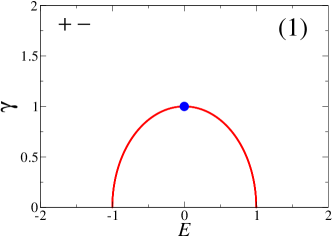
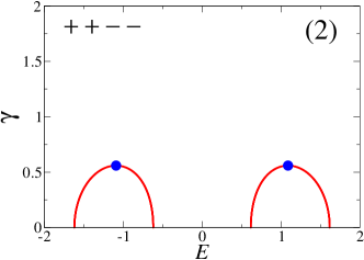
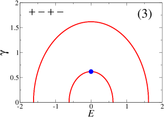
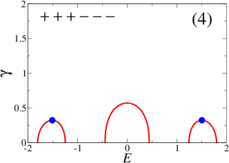
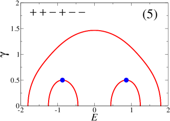
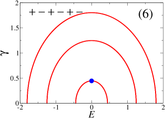
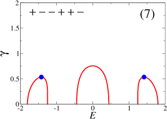
Figure 1: Real eigenvalues of the seven shortest chains in the $E$–$\gamma$ plane (see text). The full ${\cal PT}$-symmetric sequence is given in each case. All plots are at the same scale in order to facilitate the comparison between them. Blue symbols: thresholds $\gamma_{c}$ and corresponding degenerate eigenvalues.

(1) The half-sequence $(+)$ is the simplest of all. It yields the full ${\cal PT}$-symmetric sequence $(+-)$. Its characteristic polynomial is

$$P=E^{2}+\gamma^{2}-1.$$ (3.1)

The energy eigenvalues $E=\pm\sqrt{1-\gamma^{2}}$ are real for $\gamma<1$ and imaginary for $\gamma>1$. At the threshold

$$\gamma_{c}=1$$ (3.2)

there is a twofold degenerate eigenvalue at zero energy.

(2) The half-sequence $(++)$ has characteristic polynomial

$$P=E^{4}+(2\gamma^{2}-3)E^{2}+\gamma^{4}+\gamma^{2}+1.$$ (3.3)

At the threshold

$$\gamma_{c}=\frac{\sqrt{5}}{4}\approx 0.559\,016$$ (3.4)

there are degenerate energy eigenvalues at $\pm E_{c}$, with

$$E_{c}=\frac{\sqrt{19}}{4}\approx 1.089\,724.$$ (3.5)

(3) The half-sequence $(+-)$ has characteristic polynomial

$$P=E^{4}+(2\gamma^{2}-3)E^{2}+\gamma^{4}-3\gamma^{2}+1.$$ (3.6)

At the threshold

$$\gamma_{c}=\frac{\sqrt{5}-1}{2}\approx 0.618\,033$$ (3.7)

there is a twofold degenerate eigenvalue at zero energy.

(4) The half-sequence $(+++)$ has characteristic polynomial

$$P=E^{6}+(3\gamma^{2}-5)E^{4}+(3\gamma^{4}-2\gamma^{2}+6)E^{2}+\gamma^{6}+3\gamma^{4}+2\gamma^{2}-1.$$ (3.8)

At the threshold

$$\gamma_{c}\approx 0.322\,142,$$ (3.9)

obeying

$$2048\gamma_{c}^{6}+560\gamma_{c}^{4}+392\gamma_{c}^{2}-49=0,$$ (3.10)

there are degenerate energy eigenvalues at $\pm E_{c}$, with

$$E_{c}\approx 1.506\,895,$$ (3.11)

obeying

$$2048E_{c}^{6}-7216E_{c}^{4}+6632E_{c}^{2}-1831=0.$$ (3.12)

(5) The half-sequence $(++-)$ has characteristic polynomial

$$P=E^{6}+(3\gamma^{2}-5)E^{4}+(3\gamma^{4}-6\gamma^{2}+6)E^{2}+\gamma^{6}-\gamma^{4}-2\gamma^{2}-1.$$ (3.13)

At the threshold

$$\gamma_{c}=\frac{1}{2}$$ (3.14)

there are degenerate energy eigenvalues at $\pm E_{c}$, with

$$E_{c}=\frac{\sqrt{3}}{2}\approx 0.866\,025.$$ (3.15)

(6) The half-sequence $(+-+)$ has characteristic polynomial

$$P=E^{6}+(3\gamma^{2}-5)E^{4}+(3\gamma^{4}-10\gamma^{2}+6)E^{2}+\gamma^{6}-5\gamma^{4}+6\gamma^{2}-1.$$ (3.16)

At the threshold

$$\gamma_{c}=2\sin\frac{\pi}{14}\approx 0.445\,041$$ (3.17)

there is a twofold degenerate eigenvalue at zero energy.

(7) The half-sequence $(+--)$ has characteristic polynomial

$$P=E^{6}+(3\gamma^{2}-5)E^{4}+(3\gamma^{4}-6\gamma^{2}+6)E^{2}+\gamma^{6}-\gamma^{4}+2\gamma^{2}-1.$$ (3.18)

At the threshold

$$\gamma_{c}\approx 0.534\,036,$$ (3.19)

obeying

$$16\gamma_{c}^{3}+16\gamma_{c}^{2}-7=0,$$ (3.20)

there are degenerate energy eigenvalues at $\pm E_{c}$, with

$$E_{c}\approx 1.418\,436,$$ (3.21)

obeying

$$256E_{c}^{6}-768E_{c}^{4}+576E_{c}^{2}-135=0.$$ (3.22)

3.2 Panoramic overview

We now turn to an overview of the behavior of the threshold $\gamma_{c}$ for ${\cal PT}$-symmetry breaking for various kinds of configurations (periodic, random, etc.) of the optical potentials. We have run a computer routine which enumerates all the $2^{M-1}$ half-sequences of length $M$ starting with $\varepsilon_{1}=+$, up to a maximal length $M=24$, i.e., $N=48$, and determines for each sequence accurate numerical values of the threshold and of the corresponding degenerate energy eigenvalues. The most notable emerging features are illustrated in Figure 2, and will be studied in detail in the forthcoming sections. In the regime of large chains, thresholds fall off to zero, generically as a power law of the form

$$\gamma_{c}\sim\frac{1}{M^{\beta}}.$$ (3.23)

Different classes of sequences yield different decay exponents $\beta$. The smallest of all $\gamma_{c}$, decaying with exponent $\beta=2$, is reached for the diblock chains having a constant half-sequence (see black dataset and Section 4.1). The same scaling holds for all unbalanced periodic sequences with a non-zero mean value (see Section 4.2). Alternating half-sequences, as well as all balanced periodic ones with zero mean value, have thresholds falling off with exponent $\beta=1$ (see green dataset and Section 5). The mean value of $\gamma_{c}$ over all half-sequences of given length scales with exponent $\beta=3/2$. The same scaling holds for typical random sequences, i.e., for almost all half-sequences (see red dataset and Section 6). Finally, the largest threshold at fixed $M$ has an irregular dependence on $M$ and presumably also scales asymptotically as $1/M$, up to logarithmic corrections (see blue dataset and Section 7).

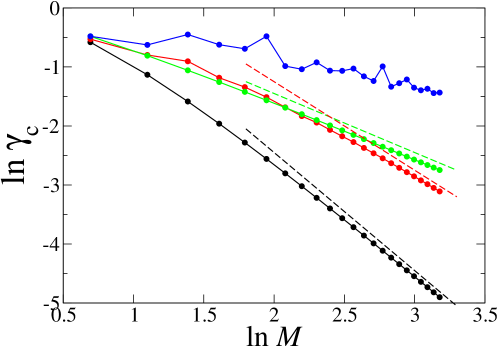
Figure 2: Log-log plot of various thresholds $\gamma_{c}$ as a function of the length $M$ of the half-sequence, ranging from 2 to 24. From bottom to top: Black: smallest $\gamma_{c}$ at fixed $M$, reached for diblock chains. Red: mean value of $\gamma_{c}$ over all half-sequences of length $M$. Green: $\gamma_{c}$ for alternating half-sequences. Blue: largest $\gamma_{c}$ at fixed $M$. Dashed lines have the theoretical slopes $\beta=2$, $3/2$ and 1, to be derived in the forthcoming sections.

4 Diblock and other unbalanced periodic chains

4.1 Diblock chains

This section is devoted to diblock chains, which are the most unbalanced of all ${\cal PT}$-symmetric chains. On a diblock chain of of length $N=2M$, the $M$ sites with gain are to the left, and the $M$ sites with loss are to the right. In other terms, the half-sequence is constant, i.e., $\varepsilon_{1}=\dots=\varepsilon_{M}=+$, and so $\varepsilon_{M+1}=\dots=\varepsilon_{2M}=-$. It is expected that the ${\cal PT}$-symmetric phase is the most fragile on these diblock chains. This is corroborated by the observation made in Section 3.2 that these chains yield the smallest threshold at fixed chain length (see black dataset in Figure 2). The latter observation will now, in turn, be made quantitative by analytical means.

Instead of using a straightforward approach borrowed from elementary Quantum Mechanics, i.e., looking for eigenfunctions of (2.1) as linear combinations of plane waves with complex wavenumbers in each block, we prefer to have recourse to the Riccati formalism introduced in Section 2.3, since the latter approach will prove more powerful in more complex situations.

The recursion (2.13) obeyed by the Riccati variables does not depend explicitly on $n$ and reads

$$R_{n}=2\cosh\mu-\frac{1}{R_{n-1}}\qquad(n=1,\dots,M),$$ (4.1)

where

$$\mu=\eta+{\rm i}q$$ (4.2)

is a complex variable such that

$$2\cosh\mu=E-{\rm i}\gamma,$$ (4.3)

i.e.,

$$E=2\cos q\;\cosh\eta,\qquad\gamma=-2\sin q\;\sinh\eta.$$ (4.4)

The fixed points of (4.1) are $R=\rme^{\pm\mu}$. Setting

$$Y_{n}=\frac{R_{n}-\rme^{-\mu}}{R_{n}-\rme^{\mu}},$$ (4.5)

the recursion (4.1) boils down to the multiplication by a constant, i.e.,

$$Y_{n}=\rme^{2\mu}Y_{n-1}.$$ (4.6)

The initial value $R_{0}=\infty$ yields $Y_{0}=1$, hence $Y_{n}=e^{2n\mu}$, and finally

$$R_{n}=\frac{\sinh(n+1)\mu}{\sinh n\mu}.$$ (4.7)

The quantization condition (2.14) therefore reads

$$\sinh(M+1)\mu\;\sinh(M+1)\mu^{\star}=\sinh M\mu\;\sinh M\mu^{\star},$$ (4.8)

i.e.,

$$\sin q\;\sin(2M+1)q+\sinh\eta\;\sinh(2M+1)\eta=0.$$ (4.9)

The above equations are exact for any finite $M$.

We are mainly interested in the scaling behavior of $\gamma_{c}$ for long chains. It turns out that the most unstable energy eigenvalues are close to the band edges ($E\to\pm 2$). Let us focus our attention onto the upper band edge ($E\to 2$, i.e., $q\to 0$) and introduce the scaling variables

$$x=(2M+1)q,\qquad g=\frac{(2M+1)^{2}}{4}\,\gamma.$$ (4.10)

We have then $(2M+1)\eta\approx(-2g/x)$, and so the quantization condition (4.9) becomes

$$\sin x\approx-\frac{2g}{x^{2}}\sinh\frac{2g}{x},$$ (4.11)

up to corrections of relative order $1/(2M+1)^{2}$.

In the absence of optical potentials ($g=0$), the r.h.s. of (4.11) vanishes. We thus obtain

$$x\approx a\pi\qquad(a=1,2,\dots),$$ (4.12)

in perfect agreement with (1.2). As the rescaled magnitude $g$ of gains and losses increases, the rescaled spectrum is more and more distorted, especially so for the very first values of $a$, as shown in Figure 3. The blue line $(g=0$) intersects the sine function at integer values of $x/\pi$ (see (4.12)). The green curve ($g=2$) yields a distorted albeit still entirely real spectrum. The red one, corresponding to

$$g_{c}\approx 4.475\,308,$$ (4.13)

is tangent to the sine function at

$$x_{c}\approx 5.331\,598$$ (4.14)

(blue symbol), where the lowest pair of eigenvalues ($a=1$ and 2) merges before becoming complex. Other mergings between $a=3$ and 4, $a=5$ and 6, and so on, take place at higher well-defined critical values of $g$.

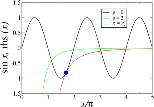
Figure 3: Graphical illustration of the threshold mechanism for the rescaled quantization condition (4.11) near the upper edge of the spectrum of long diblock chains (see text).

In brief, for long diblock chains of length $N=2M$, the threshold for ${\cal PT}$-symmetry breaking scales as

$$\gamma_{c}\approx\frac{4g_{c}}{(2M+1)^{2}}\sim\frac{g_{c}}{M^{2}}.$$ (4.15)

This provides a proof of the scaling law announced in Section 3.2, with exponent $\beta=2$, together with a prediction for the amplitude $g_{c}$. The first two pairs of degenerate eigenvalues sit very near the band edges, at $\pm E_{c}$, with

$$2-E_{c}\approx q^{2}-\eta^{2}\approx\frac{4\sigma_{c}}{(2M+1)^{2}}\sim\frac{\sigma_{c}}{M^{2}},$$ (4.16)

with

$$\sigma_{c}=\frac{x_{c}^{2}}{4}-\frac{g_{c}^{2}}{x_{c}^{2}}\approx 6.401\,903.$$ (4.17)

Both estimates (4.15) and (4.16) hold up to corrections of relative order $1/(2M+1)^{2}$.

Figure 4 provides a quantitative check of the prediction (4.15), including the order of magnitude of the corrections. The combination $(2M+1)^{2}\gamma_{c}/4$ is plotted against $1/(2M+1)^{2}$, up to $M=50$. The blue line has the theoretical intercept $g_{c}$ given in (4.13).

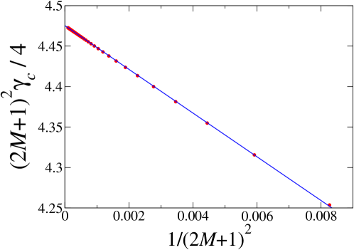
Figure 4: Red symbols: combination $(2M+1)^{2}\gamma_{c}/4$ plotted against $1/(2M+1)^{2}$, where $\gamma_{c}$ is the threshold of diblock chains. The blue line has the theoretical intercept $g_{c}$ given in (4.13).

4.2 Unbalanced periodic chains

We now turn to unbalanced periodic chains. A ${\cal PT}$-symmetric chain is said to be periodic if the half-sequence $\varepsilon_{1},\dots,\varepsilon_{M}$ is periodic, i.e., $\varepsilon_{n}=\varepsilon_{n+L}$ for some period $L\geq 1$ and all $n=1,\dots,M-L$. The motif $(\varepsilon_{1},\dots\varepsilon_{L})$ is called the unit cell of the periodic sequence. In this section we make the assumption that the periodic sequence is unbalanced, i.e., its mean value ${\overline{\varepsilon}}$ is non-zero. In the present case, we have

$${\overline{\varepsilon}}=\frac{1}{L}\sum_{n=1}^{L}\varepsilon_{n}=\frac{L_{+}-L_{-}}{L},$$ (4.18)

where $L_{+}$ and $L_{-}$ are the numbers of plus and minus signs (i.e., of sites with gain and loss) in the unit cell, with $L_{+}+L_{-}=L$.

For the time being, let us follow a heuristic line of thought. If ${\overline{\varepsilon}}$ is positive, on a spatial scale much larger than the period $L$, the left half of the chain has a roughly homogeneous gain, whereas the right half has a roughly homogeneous loss, and vice versa if ${\overline{\varepsilon}}$ is negative. Any unbalanced periodic sequence therefore amounts to an effective diblock sequence, with $\gamma$ being replaced by the effective value $\gamma_{\rm eff}=\gamma{\overline{\varepsilon}}$. This approach predicts that the threshold of a long unbalanced periodic chain is asymptotically given by the product of the expression (4.15) for diblock chains and of an amplification factor

$$f=\frac{1}{|{\overline{\varepsilon}}|}=\frac{L}{|L_{+}-L_{-}|},$$ (4.19)

depending only on the contents of the unit cell of the sequence. This reads

$$\gamma_{c}\approx\frac{4fg_{c}}{(2M+1)^{2}}\sim\frac{fg_{c}}{M^{2}}.$$ (4.20)

Consistently, diblock chains themselves can be viewed as unbalanced periodic ones with $L=L_{+}=1$, and so $f=1$. Allowing larger and larger periods, the amplification factor $f$ may become either arbitrarily close to unity or arbitrarily large: if $L\geq 3$ and $L_{\pm}=1$, we have $f=L/(L-2)$; if $L$ is odd and $L_{\pm}=(L-1)/2$, we have $f=L$.

The result (4.20) turns out to be asymptotically correct, in spite of its heuristic derivation. This will be shown in a broader setting in Section 6.1, by means of a continuum Riccati approach.

The non-trivial unbalanced chain with shortest period has $L=3$ and unit cell $(++-)$, hence $f=3$. Figure 5 provides a quantitative check of the prediction (4.20) on this example. Here again, the combination $(2M+1)^{2}\gamma_{c}/4$ is plotted against $1/(2M+1)^{2}$, up to $M=50$. Data for finite chains converge to the predicted limit value $3g_{c}\approx 13.425$ (horizontal blue line), oscillating with the period $L=3$ of the underlying sequence of gains and losses. Oscillations are damped linearly on the chosen scale.

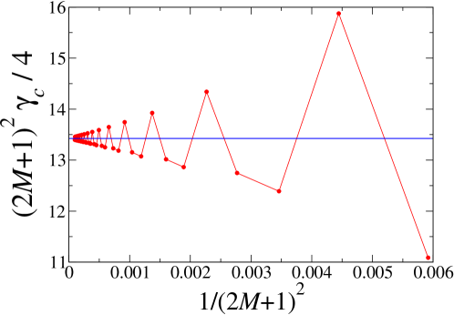
Figure 5: Red symbols: combination $(2M+1)^{2}\gamma_{c}/4$ plotted against $1/(2M+1)^{2}$, where $\gamma_{c}$ is the threshold of unbalanced chains with unit cell $(++-)$. Horizontal blue line: predicted limit value $3g_{c}\approx 13.425$.

5 Alternating and other balanced periodic chains

5.1 Alternating chains

In this section we consider alternating chains, where sites with gains and losses alternate along the chain, so that $\varepsilon_{n}=(-1)^{n}$. If the chain length $N=2M$ is even, this configuration of optical potentials obeys ${\cal PT}$-symmetry. Alternating chains are periodic with period $L=2$ and balanced, in the sense that ${\overline{\varepsilon}}=0$, so that the analysis of Section 4.2 does not apply.

Our goal is to derive the exact threshold $\gamma_{c}$ for any finite chain length $N=2M$ (see (5.11)). The analysis again relies on the Riccati formalism. The recursion (2.13) takes two different forms according to the parity of $n$:

$$R_{2p+1}=E+{\rm i}\gamma-\frac{1}{R_{2p}},\qquad R_{2p+2}=E-{\rm i}\gamma-\frac{1}{R_{2p+1}}.$$ (5.1)

These two equations can be combined, yielding

$$R_{2p+2}=\frac{(E^{2}+\gamma^{2}-1)R_{2p}-E+{\rm i}\gamma}{(E+{\rm i}\gamma)R_{2p}-1}.$$ (5.2)

Introducing the parametrization

$$E+{\rm i}\gamma=2\cos q\,\rme^{{\rm i}\theta},$$ (5.3)

i.e.,

$$E=2\cos q\;\cos\theta,\qquad\gamma=2\cos q\;\sin\theta,$$ (5.4)

and so

$$E^{2}+\gamma^{2}=4\cos^{2}q,$$ (5.5)

the fixed points of (5.2) are $R=\rme^{-{\rm i}(\theta\pm q)}$. Setting

$$Y_{n}=\frac{R_{n}-\rme^{-{\rm i}(\theta+q)}}{R_{n}-\rme^{-{\rm i}(\theta-q)}},$$ (5.6)

the recursion (5.2) boils down to

$$Y_{2p+2}=\rme^{4{\rm i}q}Y_{2p}.$$ (5.7)

The initial value $R_{0}=\infty$ yields $Y_{0}=1$, hence $Y_{2p}=e^{4{\rm i}pq}$, and finally

$$R_{2p}=\rme^{-{\rm i}\theta}\;\frac{\sin(2p+1)q}{\sin 2pq},\qquad R_{2p+1}=\rme^{{\rm i}\theta}\;\frac{\sin(2p+2)q}{\sin(2p+1)q}.$$ (5.8)

The quantization condition (2.14) reads

$$\sin(2M+1)q=0,$$ (5.9)

irrespective of $\theta$ and of the parity of $M$. This equation is considerably simpler than its counterpart (4.9) for diblock chains. It yields the explicit result

$$q=\frac{k\pi}{2M+1}\qquad(k=1,\dots,M).$$ (5.10)

For each quantized value of $q$, labelled by the integer $k$, a pair of eigenvalues merges at zero energy as $\theta\to\pi/2$, whereas $\gamma$ reaches the critical value $\gamma_{k}=2\cos q_{k}$. The pattern of real eigenvalues in the $E$–$\gamma$ plane therefore has the form of a rainbow of $M$ nested arches (see panels (1), (3) and (6) of Figure 1). The first merging event corresponds to the smallest critical value, i.e., $k=M$. We thus obtain the exact expression

$$\gamma_{c}=2\sin\frac{\pi}{2(2M+1)}$$ (5.11)

for the threshold of alternating ${\cal PT}$-symmetric chains of any finite length. We recover known values of $\gamma_{c}$ for the first values of $M$, namely $\gamma_{c}=2\sin\pi/6=1$ for $M=1$ (see (3.2)), $\gamma_{c}=2\sin\pi/10=(\sqrt{5}-1)/2$ for $M=2$ (see (3.7)), and $\gamma_{c}=2\sin\pi/14$ for $M=3$ (see (3.17)). For long alternating chains, the threshold falls off as

$$\gamma_{c}\approx\frac{\pi}{2M}.$$ (5.12)

This law of decay with exponent $\beta=1$ was announced in Section 3.2.

5.2 One example with period four

We now turn to an example of balanced periodic chains where pairs of sites with gains and losses form an alternating pattern. These chains have period $L=4$ and unit cell $(++--)$. The analysis again relies on the Riccati formalism. The recursion (2.13) reads

$$R_{4p+1}=E-{\rm i}\gamma-\frac{1}{R_{4p}},\qquad R_{4p+2}=E-{\rm i}\gamma-\frac{1}{R_{4p+1}},$$

$$R_{4p+3}=E+{\rm i}\gamma-\frac{1}{R_{4p+2}},\qquad R_{4p+4}=E+{\rm i}\gamma-\frac{1}{R_{4p+3}}.$$ (5.13)

These four equations can be combined into a recursion expressing $R_{4p+4}$ as a function of $R_{4p}$, whose expression is more intricate than (5.2). Anticipating that the threshold corresponds to a merging of eigenvalues around $E_{c}=\sqrt{2}$ (see the discussion below (5.34)), we set $E=\sqrt{2}+a$, and simplify the recursion in the scaling regime where both $a$ and $\gamma$ are small. We thus obtain

$$R_{4p+4}=\frac{(1-2\sqrt{2}\,a)R_{4p}+2{\rm i}\gamma+4a}{1+2\sqrt{2}\,a+(2{\rm i}\gamma-4a)R_{4p}}.$$ (5.14)

Introducing parameters $w$, $\phi$ and $\theta$ such that

$$a={\textstyle{\frac{1}{2}}}w\cos\phi,\qquad\gamma=w\sin\phi,\qquad\cos\theta=\frac{\cos\phi}{\sqrt{2}},$$ (5.15)

with $0<\phi<\pi$ and $\pi/4<\theta<3\pi/4$, the fixed points of (5.14) are $R=\rme^{{\rm i}(\phi\pm\theta)}$. Setting

$$Y_{4p}=\frac{R_{4p}-\rme^{{\rm i}(\phi-\theta)}}{R_{4p}-\rme^{{\rm i}(\phi+\theta)}},$$ (5.16)

the recursion (5.14) boils down to

$$Y_{4p+4}=\rme^{-2{\rm i}\lambda}Y_{4p},$$ (5.17)

with

$$\tan\lambda=2w\sin\theta.$$ (5.18)

The initial value $R_{0}=\infty$ yields $Y_{0}=1$, hence $Y_{4p}=e^{-2{\rm i}p\lambda}$, and finally

$$R_{4p}=\rme^{{\rm i}\phi}\;\frac{\sin(p\lambda-\theta)}{\sin p\lambda},\qquad R_{4p+1}=\sqrt{2}-\rme^{-{\rm i}\phi}\;\frac{\sin p\lambda}{\sin(p\lambda-\theta)}.$$ (5.19)

For $M=4p$ (and also for $M=4p+2$), the quantization condition (2.14) reads

$$\sin(p\lambda-\theta)=\pm\sin p\lambda,$$ (5.20)

yielding

$$\lambda=\frac{\theta+k\pi}{2p},$$ (5.21)

with $k$ integer. The threshold is expected to correspond to the smallest value of $\lambda$, i.e., $k=0$. It can be shown that the rescaled combinations

$$G=M\gamma,\qquad x=Ma=M(E-\sqrt{2}),$$ (5.22)

asymptotically only depend on $\theta$, according to

$$G=\frac{\theta\sqrt{-\cos 2\theta}}{\sin\theta},\qquad x=\frac{\theta\cot\theta}{\sqrt{2}}.$$ (5.23)

The threshold $\gamma_{c}$ corresponds to the point in the $x$–$G$ plane where the curve given parametrically by (5.23) has a horizontal tangent, as in Figure 1, i.e., to the maximum of the function $G(\theta)$. As $\theta$ is varied between $\pi/4$ and $3\pi/4$, $G$ reaches its maximum $G_{1}$ for $\theta_{1}$ such that $\theta_{1}=\cos 2\theta_{1}\tan\theta_{1}$, i.e., $\theta_{1}\approx 1.937\,183$, where we have

$$G_{1}\approx 1.788\,897,\qquad x_{1}\approx-0.525\,607.$$ (5.24)

For $M=4p+1$ (and also for $M=4p+3$), the quantization condition (2.14) reads

$$\sin^{2}(p\lambda-\theta)+\sin^{2}p\lambda-4\cos\theta\;\sin p\lambda\;\sin(p\lambda-\theta)=0,$$ (5.25)

whose smallest solution is

$$\lambda=\frac{\theta+\alpha}{2p},$$ (5.26)

with

$$\cos\alpha=\frac{\cos 2\theta}{\cos\theta}$$ (5.27)

and $0<\alpha<\pi$. The quantities introduced in (5.22) now read

$$G=\frac{(\theta+\alpha)\sqrt{-\cos 2\theta}}{\sin\theta},\qquad x=\frac{(\theta+\alpha)\cot\theta}{\sqrt{2}}.$$ (5.28)

The threshold is obtained by the maximization procedure applied to (5.23). As $\theta$ is varied between $\pi/4$ and $3\pi/4$, $G$ reaches its maximum $G_{2}$ for $\theta_{2}\approx 2.179\,171$, where we have

$$G_{2}\approx 2.223\,114,\qquad x_{2}\approx-1.525\,862.$$ (5.29)

To sum up, for large chains with even $M$, the threshold scales as

$$\gamma_{c}\approx\frac{G_{1}}{M},$$ (5.30)

and corresponds to two pairs of degenerate eigenvalues at $\pm E_{c}$, with

$$E_{c}\approx\sqrt{2}+\frac{x_{1}}{M},$$ (5.31)

where $G_{1}$ and $x_{1}$ are given in (5.24). For large chains with odd $M$, the threshold scales as

$$\gamma_{c}\approx\frac{G_{2}}{M},$$ (5.32)

and corresponds to two pairs of degenerate eigenvalues at $\pm E_{c}$, with

$$E_{c}\approx\sqrt{2}+\frac{x_{2}}{M},$$ (5.33)

where $G_{2}$ and $x_{2}$ are given in (5.29).

Figure 6 provides a quantitative check of the above predictions. The product $M\gamma_{c}$ is plotted against $1/M$, up to $M=100$. The upper (resp. lower) dataset corresponds to odd (resp. even) values of $M$. The blue lines have the theoretical intercepts $G_{1}$ and $G_{2}$ (see (5.24), (5.29)).

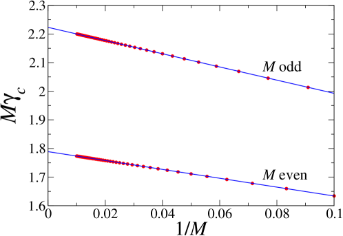
Figure 6: Red symbols: product $M\gamma_{c}$ for chains with unit cell $(++--)$, plotted against $1/M$ up to $M=100$. The upper (resp. lower) dataset corresponds to odd (resp. even) values of $M$. The blue lines have the theoretical intercepts $G_{1}$ and $G_{2}$ (see (5.24), (5.29)).

5.3 Balanced periodic chains

Let us now turn to balanced periodic chains with even period $L$ and ${\overline{\varepsilon}}=0$ (see (4.18)). Only a few general features can be stated in the present situation. This is in strong contrast with unbalanced chains, investigated in Section 4.2, where the quantitative prediction (4.20) has been derived in full generality.

The Fourier transform of a periodic chain with period $L$ is supported by all integer multiples of the reciprocal period $2\pi/L$. This singles out $L-1$ resonant energies inside the band of the free tight-binding chain, i.e.,

$$E_{a}=2\cos\frac{a\pi}{L}\qquad(a=1,\dots,L-1).$$ (5.34)

For long balanced periodic chains $(M\gg 1)$, it is expected that the energy $E_{c}$ at which the first merging of eigenvalues takes place approaches one of those resonant energies. The convention $E_{c}\geq 0$ selects $a=1,\dots,L/2$, the last case yielding $E_{c}=0$. For the alternating chain (see Section 5.1), $L=2$ and $a=1$ correctly predict $E_{c}=0$. For the chain studied in Section 5.2, $L=4$ and $a=1$ correctly predict $E_{c}=\sqrt{2}$, since $a=2$ is ruled out by symmetry. For chains with larger periods $L$, there is no systematic way of predicting the resonant energy $E_{c}$. There are actually examples where $E_{c}$ keeps varying periodically with $M$ mod $L$.

The threshold for ${\cal PT}$-symmetry breaking is expected to decay as

$$\gamma_{c}\approx\frac{G_{c}}{M}$$ (5.35)

for all balanced periodic chains. For the alternating chain (see Section 5.1), we have $G_{c}=\pi/2$ (see (5.12)). For the chain with period four studied in Section 5.2, $G_{c}$ alternates between the two numbers $G_{1}$ and $G_{2}$, according to the parity of $M$ (see (5.24), (5.29)). For chains with larger periods, the amplitude $G_{c}$ is generically expected to vary periodically with $M$ mod $L$. Many questions remain open, including whether the value $\pi/2$ obtained for alternating chains is a lower bound for $G_{c}$ and whether $G_{c}$ may become arbitrarily large.

6 Random chains

This section is devoted to random ${\cal PT}$-symmetric chains, where each symbol of the half-sequence $(\varepsilon_{1},\dots,\varepsilon_{M})$ is taken to be $\varepsilon_{n}=\pm$ with equal probabilities. Equivalently, the $2^{M}$ different half-sequences are considered as equally probable. The threshold $\gamma_{c}$ for ${\cal PT}$-symmetry breaking is now a random variable, as it depends on the chain under scrutiny. This situation has been studied by numerical means in [14].

6.1 Continuum Riccati formalism

The forthcoming analysis again relies on the Riccati formalism introduced in Section 2.3. We are mainly interested in the behavior of the threshold $\gamma_{c}$ for long random chains. In this regime, $\gamma_{c}$ is typically small, whereas the first mergings concern pairs of eigenvalues close to the band edges ($E\to\pm 2$).

Let us focus for definiteness our attention onto the upper band edge ($E\to 2$). In the vicinity of the latter, setting $E=2-q^{2}$, in the presence of small optical potentials ${\rm i}\gamma_{n}={\rm i}\gamma\varepsilon_{n}$, it is advantageous to consider the small variable

$$Z_{n}=R_{n}-1,$$ (6.1)

in terms of which the recursion (2.13) reads

$$Z_{n}=-q^{2}-{\rm i}\gamma_{n}+\frac{Z_{n-1}}{1+Z_{n-1}}=-q^{2}-{\rm i}\gamma_{n}+Z_{n-1}-Z_{n-1}^{2}+\cdots$$ (6.2)

This expansion suggests to use a continuum formalism, considering $Z(n)$ as a continuous function of the real variable $n$, obeying the Riccati differential equation

$$\frac{{\rm d}Z}{{\rm d}n}=-q^{2}-{\rm i}\gamma(n)-Z^{2},$$ (6.3)

with initial condition

$$Z(0)=\infty.$$ (6.4)

In spite of this, the function $Z(n)$ is small all over the relevant range. In particular, if the optical potential is constant, setting $\mu^{2}=-q^{2}-{\rm i}\gamma$, the solution to (6.3) reads

$$Z=\mu\mathop{{\rm cotanh}}n\mu.$$ (6.5)

To leading order as $\mu\to 0$, for fixed values of the product $n\mu$, this is in agreement with (4.7), which can be recast as

$$R_{n}=\cosh\mu+\sinh\mu\mathop{{\rm cotanh}}n\mu=1+\mu\mathop{{\rm cotanh}}n\mu+{\textstyle{\frac{1}{2}}}\mu^{2}+\cdots$$ (6.6)

Before we pursue with random chains, let us come back for a while to unbalanced periodic chains, investigated in Section 4.2. If the sequence $\varepsilon_{n}$ is periodic with period $L$ and has a non-zero mean value ${\overline{\varepsilon}}$, the continuous function $\gamma(n)$ has the same period and mean value ${\overline{\gamma}}=\gamma{\overline{\varepsilon}}$. In the situation of interest, namely sequences of length $M\gg L$, the function $Z(n)$ varies typically on a scale $M$. It is therefore slowly varying at the scale of one period, so that it is legitimate to replace $\gamma(n)$ by its mean value ${\overline{\gamma}}$. This puts the heuristic line of thought of Section 4.2 on a firmer basis.

6.2 Predictions for random chains

For long random ${\cal PT}$-symmetric chains, the function $\gamma(n)$ becomes in the continuum limit a Gaussian white noise with covariance

$${\overline{\gamma(m)\gamma(n)}}=\gamma^{2}\delta(m-n).$$ (6.7)

The continuum Riccati equation (6.3) for the function $Z(n)$ has to be integrated from $n=0$, with initial condition (6.4), to $n=M$, the length of the half-sequence, where the quantization condition (2.14) translates to

$$\mathop{{\rm Re}}Z(M)=0.$$ (6.8)

The Riccati differential equation driven by a real Gaussian white noise, i.e.,

$$\frac{{\rm d}Z}{{\rm d}x}=-q^{2}-V(x)-Z^{2},$$ (6.9)

with

$${\overline{V(x)V(y)}}=w^{2}\delta(x-y),$$ (6.10)

has a long history, dating back to pioneering studies in the 1960s of Anderson localization in a one-dimensional white-noise potential [25, 26]. The Lyapunov exponent

$$\Gamma={\overline{Z(\infty)}},$$ (6.11)

representing the inverse localization length of the model on an infinite line, obeys a scaling law of the form

$$\Gamma\approx\left({\textstyle{\frac{1}{2}}}w^{2}\right)^{1/3}\,F(x),\qquad x=\left({\textstyle{\frac{1}{2}}}w^{2}\right)^{-2/3}\,q^{2},$$ (6.12)

in the low-energy scaling regime where $q$ and $w$ are simultaneously small. The scaling function $F(x)$ is known in terms of Airy functions:

$$F(x)=\frac{{\rm Ai}(x){\rm Ai}^{\prime}(x)+{\rm Bi}(x){\rm Bi}^{\prime}(x)}{{\rm Ai}(x)^{2}+{\rm Bi}(x)^{2}}.$$ (6.13)

The result (6.12) is commonly referred to as anomalous band-edge scaling. It has been rederived several times, both in continuum and in lattice models [27, 28, 29]. Several works have been devoted to the fluctuations of the process $Z(x)$ and of closely related ones around their stationary mean value [30, 31, 32]. The mathematics involved there is quite intricate.

Fortunately enough, predictions of interest concerning the statistics of the threshold $\gamma_{c}$ of long random chains can be derived from the sole consideration of scale invariance. The continuous Riccati equations (6.3), (6.9) driven by noises obeying (6.7), (6.10) are invariant under the scaling transformation

$$(n,x)\to\frac{1}{\lambda}\,(n,x),\quad(Z,q)\to\lambda(Z,q),\quad(\gamma,w)\to\lambda^{3/2}(\gamma,w).$$ (6.14)

For the problem of Anderson localization, the scale invariance of the Riccati equation (6.9) dictates the scaling form (6.12) of the Lyapunov exponent. Of course, the determination of the exact form (6.13) of the scaling function $F(x)$ requires a more advanced analysis.

In the present context, the full scale invariance of the Riccati equation (6.3), including its boundary conditions (6.4) at $n=0$ and (6.8) at $n=M$, implies that the mean value of the threshold of long random chains scales as

$${\overline{\gamma_{c}}}\approx\frac{A}{M^{3/2}},$$ (6.15)

with a decay exponent $\beta=3/2$, as announced in Section 3.2, and that the reduced random variable

$$\xi=\frac{\gamma_{c}}{\,{\overline{\gamma_{c}}}\,}$$ (6.16)

has a well-defined limiting distribution with density $f(\xi)$, such that ${\overline{\xi}}=1$. It should be clear from the above reasoning that the latter distribution is universal, in the sense that it would hold for any symmetric, i.e., even distribution of gain/loss optical potentials $\gamma_{n}$ with finite variance. The determination of the amplitude $A$ and of the distribution $f(\xi)$ by analytical means remains a difficult open problem. We therefore have to rely on numerical analysis.

Figure 7 shows the product $M^{3/2}{\overline{\gamma_{c}}}$, plotted against $1/M$. Red circles show the outcome of a systematic enumeration of all half-chains, available up to $M=24$. These data were already presented in Section 3.2 (see red dataset in Figure 2). Blue squares show the outcome of numerical simulations with $10^{6}$ samples for $M=30$, 40 and 50. The black curve is a quadratic fit to all data points with intercept 5.660, confirming thus the scaling law (6.15) to a high degree of accuracy, and yielding the estimate

$$A\approx 5.7.$$ (6.17)

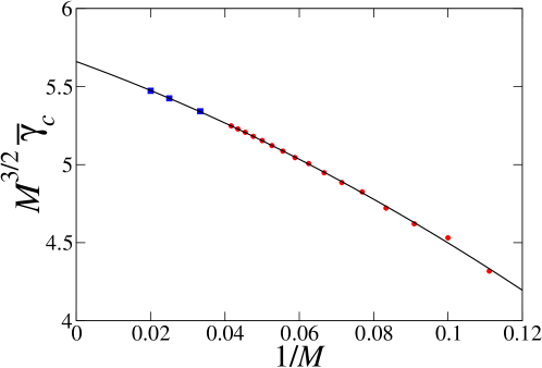
Figure 7: Plot of the product $M^{3/2}{\overline{\gamma_{c}}}$ against $1/M$. Red circles: systematic enumeration of all half-chains up to $M=24$. Blue squares: numerical simulations with $10^{6}$ samples. Black curve: quadratic fit to all data points.

Figure 8 shows the reduced combination of moments

$$Q=\frac{{\overline{\gamma_{c}^{2}}}}{({\overline{\gamma_{c}}})^{2}},$$ (6.18)

plotted against $1/M$, with the same conventions as in Figure 7. The black curve is a quadratic fit to all data points with intercept 1.351. The observed convergence to a well-defined limit provides a first quantitative piece of information on the limiting distribution $f(\xi)$, namely an estimate of its second moment,

$${\overline{\xi^{2}}}\approx 1.35,\qquad\hbox{i.e.,}\quad\mathop{{\rm var}}\xi\approx 0.35.$$ (6.19)

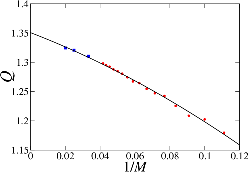
Figure 8: Plot of the quantity $Q$ defined in (6.18) against $1/M$. Same conventions as in Figure 7.

Figure 9 shows a histogram plot of the distribution of the reduced random variable $\xi$ defined in (6.16). Data are based on numerical simulations with $10^{6}$ samples for $M=40$ and 50 (see legend). Every second point of each dataset is plotted alternatively. A good collapse is observed, implying that finite-size corrections are small for the chosen chain lengths, and so that the plotted data give an accurate representation of the limiting distribution $f(\xi)$. The black curve shows a very accurate four-parameter fit of the form

$$f(\xi)\sim\exp\left(-\frac{a}{\xi^{2}}-b-c\xi-d\xi^{2}\right).$$ (6.20)

This functional form is meant to capture approximately the asymptotic behavior of the exact distribution at small and large $\xi$. For a fixed length $M$, the smallest threshold is that of diblock sequences (see Section 4.1). We have $\gamma_{c}\sim 1/M^{2}$, and so $\xi\sim 1/\sqrt{M}$, with probability $1/2^{M}$, suggesting $f(\xi)\sim\exp(-a/\xi^{2})$. The largest threshold, to be investigated in Section 7, scales as $\gamma_{c}\sim(\ln M)/M$, and so $\xi\sim\sqrt{M}\,\ln M$, again with probability $1/2^{M}$, suggesting $f(\xi)\sim\exp(-d\xi^{2})$, up to logarithmic corrections. It should however be clear that the exact distribution $f(\xi)$ is expected to be infinitely more complex than (6.20).

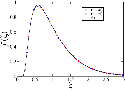
Figure 9: Histogram plot of limiting distribution $f(\xi)$ of reduced random variable $\xi$ defined in (6.16), based on numerical simulations with $10^{6}$ samples for $M=40$ and 50 (see legend). Black curve: fit of the form (6.20).

7 Most robust ${\cal PT}$-symmetric phase

In this section we consider the chains yielding the most robust ${\cal PT}$-symmetric phase, i.e., the highest threshold $\gamma_{c}$ at fixed length $M$. We describe in some detail the outcome of the systematic investigation described in Section 3.2, yielding exact data up to $M=24$, i.e., $N=48$. The value of the threshold, as well as many other characteristics of these most robust chains, exhibit an irregular dependence on the length $M$ of the half-sequence.

Let us begin with the value of the highest threshold itself. It has been shown in Section 5 that the thresholds of balanced periodic sequences fall off as $\gamma_{c}\approx G_{c}/M$ (see (5.35)), where the amplitude $G_{c}$ has a complicated dependence on the length and unit cell of the sequence. Roughly speaking, the highest threshold $\gamma_{c}$ at fixed length $M$ must be larger than all those thresholds for all periods $L\leq M$. As it turns out, $\gamma_{c}$ is larger than $1/M$ by an irregularly varying but altogether very slowly growing factor. This is demonstrated in Figure 10, showing a plot of $M$ times the highest threshold $\gamma_{c}$ against $\ln M$. These data were already presented in Section 3.2 (see blue dataset in Figure 2). The red line with slope 1.82 shows an acceptable least-square fit to the data, suggesting the behavior

$$\gamma_{c}\approx\frac{C\,\ln M}{M},\qquad C\approx 1.8.$$ (7.1)

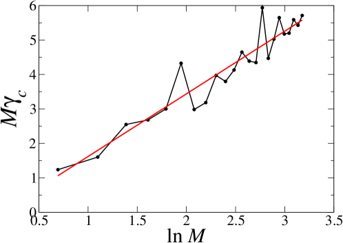
Figure 10: Plot of the product $M\gamma_{c}$ against $\ln M$, where $\gamma_{c}$ is the highest threshold at fixed length $M$, up to $M=24$. Red line with slope 1.82: least-square fit.

Table 1 provides a list of all half-sequences $(\varepsilon_{1},\dots,\varepsilon_{M})$ yielding the highest threshold shown in Figure 10, for all lengths up to $M=24$, with the convention $\varepsilon_{1}=+$ (see Section 3.1). These sequences can be viewed as consisting of alternating domains $(+-+-\dots)$ separated by domain walls, in the words of magnetism, denoted by vertical bars. The number of domain walls and their positions optimize the value of the threshold. We have not succeeded in identifying any pattern in those optimal positions.

In order to illustrate the complexity of the dependence of $\gamma_{c}$ on the positions of the domain walls, we consider in C alternating chains having a single pair of ${\cal PT}$-related domain walls between sites $K$ and $K+1$ and between sites $2M-K$ and $2M-K+1$. Already in this situation, the threshold is found to have an intricate asymptotic dependence on the ratio $\alpha=K/M$, involving four different regimes. This threshold is always enhanced by the presence of the domain walls, with respect to that of pristine alternating chains (see (5.12)). The enhancement factor takes its maximal value 3 for $\alpha=1/3$.

$M$	$\varepsilon_{1},\dots,\varepsilon_{M}$
1	$+$
2	$+-$
3	$+-|-$
4	$+|+-+$
5	$+-|-+-$
6	$\left\{\matrix{+-+|+-|-\cr+-|-+-+\cr+|+-+-+}\right.$
7	$+-|-+-+-$
8	$+-|-+-+-+$
9	$+-|-+-+-+|+$
10	$+-+|+-+-+-+$
11	$+-+|+-+-+-+-$
12	$+|+-+-|-+-+-+-$
13	$+-+-+-+|+-+-|-+$
14	$+-+-+-|-+-+|+-|-+$
15	$+-+|+-|-+-+-+|+-+-$
16	$\left\{\matrix{+|+-+-+-+-|-|-+|+-+-\cr+|+-+-+-+-|-+|+|+-+-}\right.$
17	$+-+-+-+|+-|-+|+-+-|-+$
18	$+-+|+-|-+-+|+-+-+-|-+-$
19	$\left\{\matrix{+|+-+-+-+-+-|-|-+|+-+-+\cr+|+-+-+-+-+-|-+|+|+-+-+}\right.$
20	$+|+-+-+-|-+|+-+-|-+|+-+|+-$
21	$+-|-+|+-|-+|+-+-|-+-+|+-+-+$
22	$+-+|+-+-+-+-+-|-+|+-+-|-+|+$
23	$+-+-+-+|+-|-+|+-|-+-+|+-+-|-+$
24	$+|+-+-+-|-+-+-+-+-+|+-|-+-+|+$

Table 1: Half-sequences yielding the highest thresholds $\gamma_{c}$ at fixed length $M$, up to $M=24$. Vertical bars: domain walls between alternating domains.

Some degeneracies can be seen in Table 1. For $M=6$, three different half-sequences yield the maximal $\gamma_{c}=1/2$, with mergings occurring at different critical energies (see below). For $M=16$ and $M=19$, two different half-sequences yield the same maximal threshold and mergings at the same critical energies. The threshold $\gamma_{c}$ generically corresponds to the appearance of two twofold degenerate eigenvalues at opposite energies $\pm E_{c}$, where $E_{c}>0$ has itself an irregular dependence on $M$ (data not shown). For $M=2$, 7, 8, 12 and 21, there is a single twofold degenerate eigenvalue at zero energy.

The case $M=6$ is special in several regards. Three distinct half-sequences, listed in Table 1, yield the highest threshold $\gamma_{c}=1/2$. This simple value allows for an analytical study of the corresponding energy spectra. For the first half-sequence $(+-++--)$, the first mergings occur at $\pm E_{c}$, with

$$E_{c}=\frac{\sqrt{7}}{2}\approx 1.322\,875.$$ (7.2)

For the second half-sequence $(+--+-+)$, four mergings occur simultaneously at $\pm E_{c1}$ and $\pm E_{c2}$, with

$$E_{c1}=\frac{\sqrt{5-2\sqrt{5}}}{2}\approx 0.363\,271,\quad E_{c2}=\frac{\sqrt{5+2\sqrt{5}}}{2}\approx 1.538\,841.$$ (7.3)

For the third half-sequence $(++-+-+)$, which is the only unbalanced one, the first mergings occur at $\pm E_{c}$, with

$$E_{c}=\frac{\sqrt{3}}{2}\approx 0.866\,025.$$ (7.4)

8 Discussion

This paper has been devoted to non-Hermitian ${\cal PT}$-symmetric tight-binding chains of $N=2M$ sites, where gain/loss optical potentials of equal magnitudes, of the form ${\rm i}\gamma\varepsilon_{n}$ with $\varepsilon_{n}=\pm 1$, are distributed over all sites in a periodic, random, or any other fashion. We have provided a systematic study of the threshold $\gamma_{c}$ for ${\cal PT}$-symmetry breaking, with the main emphasis being on the dependence of $\gamma_{c}$ on the chain length for various classes of configurations of optical potentials. Our main findings are summarized in the panoramic overview of the asymptotic behavior of $\gamma_{c}$ for various classes of chains given in Section 3.2 (see Figure 2). The threshold generically falls off as a power of the chain length, i.e.,

$$\gamma_{c}\sim\frac{1}{M^{\beta}}.$$ (8.1)

The decay exponent $\beta$ depends on the configuration of optical potentials. The largest exponent $\beta=2$ is reached for diblock chains, and more generally for all unbalanced periodic chains, i.e., periodic configurations of optical potentials where each half of the chain has on average either gain or loss. The smallest exponent $\beta=1$ is attained for alternating chains, and more generally for all balanced periodic chains, i.e., periodic configurations of optical potentials whose spatial average over one period vanishes. For random sequences of optical potentials with zero average and finite variance, the threshold $\gamma_{c}$ is itself a random variable, whose mean value decays with exponent $\beta=3/2$, whereas the fluctuations around this mean value obey a universal distribution $f(\xi)$.

These results have been corroborated and made quantitative by detailed analytical studies performed in Sections 4 to 6. This analysis relies on concepts and techniques from the physics of one-dimensional disordered systems, including the transfer-matrix approach and the discrete Riccati formalism.

The above results can be put in a broader context as follows. Consider the sum

$$S=\varepsilon_{1}+\cdots+\varepsilon_{M}$$ (8.2)

of all reduced optical potentials over the left half of the chain, and assume that this sum grows as

$$S\sim M^{\omega},$$ (8.3)

with a wandering exponent in the range $0\leq\omega\leq 1$. The three classes of configurations of optical potentials recalled above respectively yield $\beta=2$, 1 and 3/2, whereas they clearly obey (8.3) with $\omega=1$, 0 and 1/2. This observation suggests the hyperscaling relation

$$\beta=\omega+1.$$ (8.4)

This relation provides a quantitative form of the rule of thumb according to which the more the sites with gain and loss are well mixed along the chain, the more robust the corresponding ${\cal PT}$-symmetric phase. A large class of deterministic aperiodic sequences have non-trivial wandering exponents $\omega$, besides the three classical values recalled above [33, 34, 35, 36]. The relation (8.4) certainly holds in those cases as well, thus predicting a whole zoo of non-trivial asymptotic decay exponents $\beta$.

The chains yielding the most robust ${\cal PT}$-symmetric phase, i.e., the highest threshold $\gamma_{c}$ at fixed chain length, have been investigated by means of a systematic enumeration up to $M=24$, i.e., $N=48$ (see Section 7). Both the optimal $\gamma_{c}$ itself and the sequences responsible for it exhibit an irregular dependence on $M$. The highest threshold presumably falls off asymptotically as $(\ln M)/M$. These logarithmic corrections somehow represent an exception to the above rule of thumb. The chains yielding the optimal thresholds indeed contain several domain walls, i.e., pairs of consecutive sites with gain or loss. They are therefore slightly less well mixed than pristine alternating ones, whereas the corresponding thresholds are larger.

To close, it would certainly be interesting to extend at least some aspects of the present study to more complex situations, including e.g. a periodic, quasiperiodic or random modulation of on-site energies and/or hopping rates, or quasi-one-dimensional geometries such as ladders, exhibiting either internal band gaps or flat bands.

Appendix A First-order perturbation theory

In this appendix we derive within the framework of first-order perturbation theory the spectrum of the tight-binding equation

$$\psi_{n-1}+\psi_{n+1}+{\rm i}\gamma_{n}\psi_{n}=E\psi_{n},$$ (1.1)

with Dirichlet boundary conditions, for an arbitrary sequence of purely imaginary optical potentials $\gamma_{1},\dots,\gamma_{2M}$. Our goal is to show that all energy levels remain real within this framework if and only if the sequence $\gamma_{n}$ is ${\cal PT}$-symmetric.

In the absence of optical potentials, the non-degenerate energy eigenvalues and normalized eigenstates read

$$E_{a}=2\cos\frac{a\pi}{2M+1}\qquad(a=1,\dots,2M),$$ (1.2)

$$\psi_{a,n}=\sqrt{\frac{2}{2M+1}}\sin\frac{an\pi}{2M+1}.$$ (1.3)

To first order in the optical potentials, the energy eigenvalues read $E_{a}+{\rm i}\Gamma_{a}$, with

$$\Gamma_{a} = \sum_{n=1}^{2M}\gamma_{n}\psi_{a,n}^{2}$$ (1.4)

$$= \frac{2}{2M+1}\sum_{n=1}^{M}\left(\gamma_{n}+\gamma_{2M+1-n}\right)\,\sin^{2}\!\frac{an\pi}{2M+1}.$$

If the sequence $\gamma_{1},\dots,\gamma_{2M}$ is ${\cal PT}$-symmetric, obeying

$$\gamma_{2M+1-n}=-\gamma_{n},$$ (1.5)

all the sums in the parentheses in the last line of (1.4) vanish, and therefore all the first-order imaginary parts $\Gamma_{a}$ vanish, suggesting the existence of a non-zero threshold $\gamma_{c}$ for ${\cal PT}$-symmetry breaking.

The proof of the reciprocal proceeds as follows. The first-order imaginary parts (1.4) obey the mirror symmetry $\Gamma_{2M+1-a}=\Gamma_{a}$, so that it is sufficient to consider $a=1,\dots,M$. Requesting $\Gamma_{a}=0$ for $a=1,\dots,M$ yields a system of $M$ linear equations for the $M$ unknown quantities $(\gamma_{n}+\gamma_{2M+1-n})$ for $n=1,\dots,M$. The corresponding determinant,

$$D_{M}=\det A,$$ (1.6)

with

$$A_{an}=\sin^{2}\!\frac{an\pi}{2M+1}\qquad(a,n=1,\dots,M),$$ (1.7)

is non-zero. It can indeed be evaluated by using $D_{M}^{2}=(\det A)^{2}=\det(A^{2})$. This is useful since the entries of the matrix $A^{2}$ have simple expressions [37, 38]. Expanding the sines into complex exponentials and performing the sums, we indeed obtain after some algebra

$$(A^{2})_{ab}=\frac{2M+1}{8}\left(1+{\textstyle{\frac{1}{2}}}\delta_{ab}\right).$$ (1.8)

The determinant of a matrix of size $M\times M$ with entries $\lambda+\mu\delta_{ab}$ reads $\mu^{M-1}(M\lambda+\mu)$. We thus obtain

$$|D_{M}|=\frac{(2M+1)^{(M+1)/2}}{2^{2M}}.$$ (1.9)

The sign of $D_{M}$ is not predicted by this approach. It depends periodically on $M$ mod 4.

To sum up, $\Gamma_{a}=0$ for all $a$ implies $\gamma_{n}+\gamma_{2M+1-n}=0$ for all $n$, i.e., ${\cal PT}$-symmetry. This completes the proof.

Appendix B Chain of length four with arbitrary gains and losses

In this appendix we consider the tight-binding equation

$$\psi_{n-1}+\psi_{n+1}+{\rm i}\gamma_{n}\psi_{n}=E\psi_{n}$$ (2.1)

on a ${\cal PT}$-symmetric chain of length $N=2M=4$, with arbitrary imaginary optical potentials, obeying

$$\gamma_{3}=-\gamma_{2},\qquad\gamma_{4}=-\gamma_{1}.$$ (2.2)

The first two optical potentials $\gamma_{1}$ and $\gamma_{2}$ are kept as free parameters.

The quantization condition (2.14) is expressed by the characteristic polynomial

$$P=E^{4}+(\gamma_{1}^{2}+\gamma_{2}^{2}-3)E^{2}+(\gamma_{1}\gamma_{2}+\gamma_{1}+1)(\gamma_{1}\gamma_{2}-\gamma_{1}+1).$$ (2.3)

This polynomial has a rich bifurcation diagram shown in Figure 11.

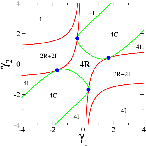
Figure 11: Bifurcation diagram of the ${\cal PT}$-symmetric chain of length $N=2M=4$ in the $\gamma_{1}$–$\gamma_{2}$ plane (see text). ${\cal PT}$-symmetry is unbroken in the central region marked 4R.

There is a twofold degenerate eigenvalue at zero energy on the red curves, i.e., for

$$(\gamma_{1}\gamma_{2}+\gamma_{1}+1)(\gamma_{1}\gamma_{2}-\gamma_{1}+1)=0.$$ (2.4)

There are two twofold degenerate eigenvalues at $\pm E_{c}\neq 0$ (either real or imaginary) on the green curves, i.e., for

$$(\gamma_{1}^{2}-\gamma_{2}^{2})^{2}-2(\gamma_{1}+\gamma_{2})(\gamma_{1}+3\gamma_{2})+5=0.$$ (2.5)

The red and green curves have four contact points (blue symbols), at

$$(\gamma_{1}\approx 1.683\,771,\quad\gamma_{2}\approx 0.406\,095),$$

$$(\gamma_{1}\approx-0.371\,506,\quad\gamma_{2}\approx 1.691\,739),$$ (2.6)

and their opposites, where the characteristic polynomial has a fourfold degenerate eigenvalue at zero energy. These four points are cocyclic, obeying $\gamma_{1}^{2}+\gamma_{2}^{2}=3$.

The above curves define various regions in the $\gamma_{1}$–$\gamma_{2}$ plane. The structure of the energy spectrum is given in each region, with R, I and C denoting real, imaginary and generic complex eigenvalues. For instance, 2R+2I means two opposite non-zero real eigenvalues and two opposite non-zero purely imaginary ones.

${\cal PT}$-symmetry is unbroken whenever all eigenvalues are real, i.e., in the central region marked 4R. This quadrangular region is bounded by two red arcs and two green ones meeting at the four blue contact points. The predictions (3.4) and (3.7) for the thresholds of binary chains with half-sequences $(++)$ and $(+-)$ can be respectively recovered by intersecting one of the green arcs with the bisector line of equation $\gamma_{2}=\gamma_{1}$ and of the red ones with the bisector line of equation $\gamma_{2}=-\gamma_{1}$.

Appendix C Alternating chains with a single pair of domain walls

This appendix is devoted to almost pristine alternating chains of length $N=2M$ having a single pair of domain walls at ${\cal PT}$-related positions between sites $K$ and $K+1$ and between sites $2M-K$ and $2M-K+1$. The corresponding half-sequence reads

$$\varepsilon_{n}=\left\{\matrix{(-1)^{n}\hfill&(n=1,\dots,K),\hfill\cr(-1)^{n-1}\hfill&(n=K+1,\dots,M).}\right.$$ (3.1)

For instance, for $M=5$ and $K=2$, the half-sequence reads $(-+|+-+)$, and so the full sequence reads $(-+|+-+-+-|-+)$, where vertical bars denote domain walls.

The forthcoming analysis, including notations, closely follows Section 5.1, which was devoted to pristine alternating chains. For definiteness we restrict ourselves to the case where $M$ and $K$ are even. The expressions (5.8) of the Riccati variables still hold for $n=1,\dots,K$. We have therefore in particular

$$R_{K}=\rme^{-{\rm i}\theta}\;\frac{\sin(K+1)q}{\sin Kq}.$$ (3.2)

For $n=K+1,\dots,M$, the recursion obeyed by the Riccati variables $R_{n}$ is obtained by changing $\gamma$ and $\theta$ into their opposites in (5.1) and (5.2). In particular, the variables

$$Y_{n}=\frac{R_{n}-\rme^{{\rm i}(\theta-q)}}{R_{n}-\rme^{{\rm i}(\theta+q)}}$$ (3.3)

still obey the recursion (5.7). We have therefore

$$Y_{M}=\rme^{2{\rm i}q(M-K)}Y_{K}.$$ (3.4)

Using the three above equations, we obtain

$$R_{M}=\rme^{{\rm i}\theta}\;\frac{c_{M}-c_{M+2}+{\rm i}\tan\theta\left(c_{M}+c_{M+2}-2c_{M-2K}\right)}{c_{M-1}-c_{M+1}+{\rm i}\tan\theta\left(c_{M-1}+c_{M+1}-2c_{M-2K-1}\right)},$$ (3.5)

with the shorthand notation $c_{n}=\cos nq$. Finally, the quantization condition (2.14) simplifies to

$$4\sin^{2}\theta \,\sin Kq\,\sin(K+1)q\,\sin(2M-2K)q$$ (3.6)

$$+\sin^{2}q\,\sin(2M+1)q=0.$$

The above equation is exact for any even integers $M$ and $K$.

For long chains, where both $M$ and $K$ are large, the threshold for ${\cal PT}$-symmetry breaking scales as

$$\gamma_{c}\approx\frac{G_{c}(\alpha)}{M},$$ (3.7)

where the numerator has a rich dependence on the ratio

$$\alpha=\frac{K}{M},$$ (3.8)

as announced in Section 7. The amplitude $G_{c}(\alpha)$ is always larger than that of pristine alternating chains (see (5.12)), which is recovered for $\alpha\to 0$ and $\alpha\to 1$. The effect of the domain walls indeed disappears in both limits, where they either attain the endpoints of the chain or annihilate each other in the middle. The threshold amplification is maximal for $\alpha\to(1/3)_{-}$, where we have $G_{c}((1/3)_{-})/G_{c}(0)=3$. Figure 12 shows a plot of $G_{c}(\alpha)$ against $\alpha$. Numerical results for the thresholds for $M=60$ and all possible positions of the domain walls are compared to the exact expression of $G_{c}(\alpha)$, involving four different regimes, to be successively investigated below.

• Regime (1) holds for $0<\alpha<1/3$. The amplitude increases from $G_{c}(0)=\pi/2\approx 1.570\,796$ to $G_{c}((1/3)_{-})=3\pi/2\approx 4.712\,388$.

• Regime (2) holds for $1/3<\alpha<\alpha_{2}$. At $\alpha=1/3$ the amplitude drops discontinuously to $G_{c}((1/3)_{+})=3\pi\sqrt{3}/4\approx 4.081\,048$. We have $\alpha_{2}\approx 0.583\,417$ and $G_{c}(\alpha_{2})\approx 2.697\,312$.

• Regime (3) holds for $\alpha_{2}<\alpha<\alpha_{3}$. The amplitude is continuous at $\alpha_{2}$ and at $\alpha_{3}$, with $\alpha_{3}\approx 0.776\,365$ and $G_{c}(\alpha_{3})\approx 2.841\,880$.

• Regime (4) holds for $\alpha_{3}<\alpha<1$. The amplitude decreases from $G_{c}(\alpha_{3})$ to $G_{c}(1)=\pi/2\approx 1.570\,796$.

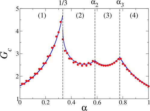
Figure 12: Plot of the amplitude $G_{c}(\alpha)$ against the reduced position $\alpha$ of the left domain wall. Full curves: analytical asymptotic predictions (3.10), (3.13), (3.17), (3.11) in the four regimes. Symbols: data for $M=60$ and all possible positions of the domain walls.

Analytical expressions of the amplitude $G_{c}(\alpha)$ in each regime can be derived by zooming onto the exact quantization condition (3.6) in appropriate ranges.

In Regimes (1) and (4), the first merging takes place at zero energy. This corresponds to $\theta=\pi/2$, whereas $q=\pi/2-\eta$, and so $\gamma_{c}\approx 2\eta$, with $\eta\sim 1/M$. The quantization condition (3.6) asymptotically becomes

$$\cos(1-2\alpha)G_{c}=0.$$ (3.9)

The amplitude $G_{c}(\alpha)$ is the smallest positive solution to the above equation. We thus obtain the explicit expressions

$$G_{c}(\alpha)=\frac{\pi}{2(1-2\alpha)}\quad\hbox{in Regime~{}(1)},$$ (3.10)

$$G_{c}(\alpha)=\frac{\pi}{2(2\alpha-1)}\quad\hbox{in Regime~{}(4)}.$$ (3.11)

In Regime (2), the first mergings take place near zero energy. This corresponds to $q=\pi/2-\eta$ with $\eta\sim 1/M$ and $\theta$ variable, and so $E_{c}\approx 2\eta\cos\theta$ and $\gamma_{c}\approx 2\eta\sin\theta$. Introducing the product $x=2M\eta$, the quantization condition (3.6) asymptotically becomes

$$2\sin^{2}\theta\,\sin\alpha x\,\sin(1-\alpha)x+\cos x=0.$$ (3.12)

The threshold is obtained by the maximization procedure applied to (5.23), yielding

$$G_{c}(\alpha)=\mathrel{\mathop{\;\max\;}\limits_{x}}x\sqrt{-\frac{\cos x}{2\sin\alpha x\,\sin(1-\alpha)x}},$$ (3.13)

where the maximum is taken over $x$ in the range $\pi/2<x<3\pi/2$ at fixed $\alpha$. The amplitude takes its minimal value $G_{c}(1/2)\approx 2.529\,882$ for $\alpha=1/2$, i.e., when the left domain wall is in the middle of the half-sequence. It has a square-root endpoint singularity at $\alpha=1/3$, below which Regime (1) takes over. Setting

$$\alpha=\frac{1}{3}+\delta,$$ (3.14)

the maximum takes place for

$$x\approx\frac{3\pi}{2}-\frac{3\pi\sqrt{3\delta}}{4}$$ (3.15)

and reads

$$G_{c}\approx\frac{3\pi\sqrt{3}}{4}-\frac{9\pi\sqrt{\delta}}{4}.$$ (3.16)

In Regime (3), the first mergings take place near the band edges. This corresponds to both $q$ and $\theta$ scaling as $1/M$. Introducing the product $x=Mq$, we obtain the asymptotic prediction

$$G_{c}(\alpha)=\mathrel{\mathop{\;\max\;}\limits_{x}}\frac{x}{\sin\alpha x}\sqrt{-\frac{\sin 2x}{\sin 2(1-\alpha)x}},$$ (3.17)

where the maximum is taken over $x$ in the range $\pi/2<x<\pi$ at fixed $\alpha$. The amplitude takes its minimal value $G_{c}(2/3)\approx 2.493\,125$ for $\alpha=2/3$.

References

References

- [1] Ashida Y, Gong Z and Ueda M 2020 Adv. Phys. 69 249–435
- [2] Bender C M and Boettcher S 1998 Phys. Rev. Lett. 80 5243–5246
- [3] Bender C M, Brody D C and Jones H F 2002 Phys. Rev. Lett. 89 270401
- [4] Zinn-Justin J and Jentschura U D 2010 J. Phys. A 43 425301
- [5] Bender C M 2007 Rep. Prog. Phys. 70 947–1018
- [6] Bender C M 2016 Europhysics News 47 17–20
- [7] El-Ganainy R, Makris K G, Khajavikhan M, Musslimani Z H, Rotter S and Christodoulides D N 2018 Nature Phys. 14 11–19
- [8] Bendix O, Fleischmann R, Kottos T and Shapiro B 2009 Phys. Rev. Lett. 103 030402
- [9] Jin L and Song Z 2009 Phys. Rev. A 80 052107
- [10] Joglekar Y N, Scott D, Babbey M and Saxena A 2010 Phys. Rev. A 82 030103
- [11] Joglekar Y N and Barnett J L 2011 Phys. Rev. A 84 024103
- [12] Mejía-Cortés C and Molina M I 2015 Phys. Rev. A 91 033815
- [13] Molina M I 2015 Phys. Rev. A 92 063813
- [14] Harter A K, Assogba Onanga F and Joglekar Y N 2018 Sci. Rep. 8 44
- [15] Ortega A, Stegmann T, Bene L and Larralde H 2020 J. Phys. A 53 445308
- [16] Longhi S 2014 Optics Lett. 39 1697–1700
- [17] Elenewski J E and Chen H 2014 Phys. Rev. B 90 085104
- [18] Garmon S, Gianfreda M and Hatano N 2015 Phys. Rev. A 92 022125
- [19] Zhang L L and Gong W J 2017 Phys. Rev. A 95 062123
- [20] Crisanti A, Paladin G and Vulpiani A 1992 Products of Random Matrices in Statistical Physics Springer Series in Solid-State Sciences (Berlin: Springer)
- [21] Luck J M 1992 Systèmes désordonnés unidimensionnels (Saclay: Collection Aléa)
- [22] Pendry J B 1994 Adv. Phys. 43 461
- [23] Comtet A, Texier C and Tourigny Y 2013 J. Phys. A 46 254003
- [24] Comtet A and Tourigny Y 2017 Impurity models and products of random matrices Stochastic Processes and Random Matrices ed Schehr G, Altland A, Fyodorov Y V, O’Connell N and Cugliandolo L F (Oxford: Oxford University Press) (Preprint arXiv:1601.01822)
- [25] Frisch H L and Lloyd S P 1960 Phys. Rev. 120 1175–1189
- [26] Halperin B I 1965 Phys. Rev. 139 A104–A117
- [27] Derrida B and Gardner E 1984 J. Phys. (France) 45 1283–1295
- [28] Izrailev F M, Ruffo S and Tessieri L 1998 J. Phys. A 31 5263–5270
- [29] Comtet A, Luck J M, Texier C and Tourigny Y 2013 J. Stat. Phys. 150 13–65
- [30] Schomerus H and Titov M 2002 Phys. Rev. E 66 066207
- [31] Ramola K and Texier C 2014 J. Stat. Phys. 157 497–514
- [32] Fyodorov Y V, Le Doussal P, Rosso A and Texier C 2018 Ann. Phys. 397 1–64
- [33] Godrèche C and Luck J M 1992 Phys. Rev. B 45 176–185
- [34] Luck J M 1993 Europhys. Lett. 24 359–364
- [35] Queffélec M 2010 Substitution Dynamical Systems, Spectral Analysis 2nd ed (New York: Springer)
- [36] Baake M and Grimm U 2013 Aperiodic Order vol 1 (Cambridge: Cambridge University Press)
- [37] Krapivsky P L, Luck J M and Mallick K 2015 J. Phys. A 48 475301
- [38] Luck J M 2016 J. Phys. A 49 115303