Computing the Probability of a Financial Market Failure: A New Measure of Systemic Risk

Abstract

This paper characterizes the probability of a market failure defined as the default of two or more globally systemically important banks (G-SIBs) in a small interval of time. The default probabilities of the G-SIBs are correlated through the possible existence of a market-wide stress event. The characterization employs a multivariate Cox process across the G-SIBs, which allows us to relate our work to the existing literature on intensity-based models. Various theorems related to market failure probabilities are derived, including the probability of a market failure due to two banks defaulting over the next infinitesimal interval, the probability of a catastrophic market failure, the impact of increasing the number of G-SIBs in an economy, and the impact of changing the initial conditions of the economy’s state variables. We also show that if there are too many G-SIBs, a market failure is inevitable, i.e., the probability of a market failure tends to 1.

Key words: Systemic risk, market failure probabilities, G-SIBs, multivariate Cox processes.

1 Introduction and Summary

For regulators, characterizing the probability of a financial market failure, or systemic risk, is important because such a characterization enables them to understand how their regulatory actions affect its magnitude. In this regard, numerous systemic risk measures have been proposed in the literature, each with associated benefits and limitations. For literature reviews of the existing collection of systemic risk measures, see Bisias et al., (2012) and Engle, (2018). This paper provides another measure of systemic risk, different from the existing set. According to the systemic risk measure taxonomies in Bisias et al., (2012), ours is a macroeconomic or macroprudential measure, which is a based on a default intensity model. As such, it is a forward-looking measure, which satisfies the following characteristics:

1. it is consistent with the economic theories relating to the causes of financial market failures (macroeconomic),

2. it uses the existing regulatory designations of globally systemically important banks (G-SIBs), financial institutions that are “too big to fail” (macroeconomic),

3. it can be estimated using existing hazard rate methodologies (default intensity), and

4. it facilitates quantifying the impact of regulatory policy changes on systemic risk (macroprudential).

Our measure of systemic risk is the probability that any two G-SIBs default at the “same time.” A G-SIB is any financial institution that has been designated by the Financial Stability Board (FSB) as large enough such that if it fails, its failure affects the health of the financial system. Operationally, a bank is designated as a G-SIB if various indicators of its financial health, in aggregate, exceed some threshold (see FSB 2020 and BIS 2014). There were 30 such G-SIBs designated by the FSB in 2020. By the “same time” we mean within a short time period of each other, say 1 week.

The idea underlying our measure is that if one G-SIBs fails, regulators can manage the resulting crisis to ensure that a market wide failure does not occur. Examples of such past episodes include the failure of Long Term Capital Management in 1998 and Lehman Brothers, together with Bear Sterns, in 2008. For both of these episodes, regulators were able to manage the crisis and prevent a market-wide failure. However, if two (or more) G-SIBs fail within a short time period of each other, then our measure asserts that the crisis is uncontrollable by regulators and the market fails.

Our measure is consistent with economic theories of market failures because, in a reduced form fashion, it implicitly includes the causes for the failure, e.g. the “drying-up” of short-term funding, the bursting of an asset price bubble, or the propagation of defaults in a network of banks due to inter-linked funding (see Allen & Carletti, (2013), Acemoglu et al., (2015), Jarrow & Lamichhane, (2021)). And, it also explicitly incorporates the marginal impact of a G-SIBs’s default on the probability of a financial market failure (see Acharya et al., (2009) for related discussion).

By its definition, our measure builds upon the fundamental analysis already done by regulators in identifying financial institutions that are G-SIBs. In the identification of G-SIBs, regulators include public information (market prices, macroeconomic statistics, a financial institution’s annual reports), non-public information available via the regulatory channel, and expert judgement (see BIS 2014). The use of the G-SIB designations as a basis for our systemic risk measure, which include this non-public information and expert judgement, yields an additional benefit not available with the use of publicly available information alone.

Our measure can also be estimated due to its construction, because the probability of a market failure incorporates the existing marginal probabilities of a G-SIB defaulting. These probabilities can be obtained as in the existing hazard rate estimation literature, see Chava & Jarrow, (2004), Campbell et al., (2008), Shumway, (2001). The data necessary to compute these marginal default probabilities is publicly available, and they consist of historical data on financial institutions defaults, annual reports (balance sheet data), and market variables (prices and macroeconomic statistics). Finally, given the analytic representation of our systemic risk measure, it is easy to compute the impact of a regulatory policy change on the probability of a market failure, e.g., such regulatory actions might be the breaking-up of a G-SIB or the increase in a G-SIB’s capital. These regulatory changes correspond to modifying various input variables underlying the market failure probabilities and determining their impact on the resulting value.

Our paper falls within the credit risk literature studying correlated firm defaults. There are two approaches in this literature. One approach is to have the firms’ default intensities dependent on each other, either through information events or counterparty risk. This method typically uses Cox processes with independent default indicators implying simultaneously occurring default times happen with zero probability. The second approach extends these models to allow for a strictly positive probability of simultaneous defaults. Our paper lies within the second class. Papers in both of these genres include Giesecke, (2003), Lindskog & McNeil, (2003), Bielecki et al., (2013), Bielecki & Rutkowski, (2003), Brigo et al., (2007a), (2007b), Coculescu, (2022), El Karoui et al., (2017), and Liang & Wang, (2012).

The mathematical model in our paper can be viewed as a special case of that presented in Bielecki et al., (2013). A key difference is that we apply our model to characterize systemic risk, while Bielecki et al., (2013) study the pricing of basket credit derivatives, in particular credit default obligations (CDOs). In addition, as previously noted, we derive a collection of results related to the probability of a systemic risk event occurrence that are new to this literature.

An outline for the paper is as follows. Section 2 presents the model, while section 3 contains the key theorems. Section 4 provides comparative statics and concludes the paper.

2 The Model

The following model is based on Protter & Quintos, (2021). Fix a filtered probability space $\left(\Omega,\mathcal{F},\mathbb{P},\mathbb{F}\right)$ satisfying the usual conditions and large enough to support an $\mathbb{R}^{d}$ - valued right continuous with left limits existing stochastic process $X=\{X_{t},t\geq 0\}$ and $K+1$ independent exponential random variables each with parameter $1$, i.e. $(Z_{i},i=0,...,K)$. It must be noted that the $K+1$ exponential random variables are independent of each other and of the stochastic process $X$.

Consider a financial market that contains $i=1,...,K$ financial institutions that are classified as G-SIBs, i.e. too big to fail. There can be numerous other financial institutions in the market, but their existence will not be explicitly included in our systemic risk measure. However, these non-G-SIBs are implicitly included as will be subsequently noted.

The stochastic process $X$ represents a vector of state variables characterizing the health of the economy and the $K$ G-SIBs. It includes macro variables such as the inflation rate, the unemployment rate, the level of interest rates, and G-SIB specific balance sheet quantities such as their capital ratios.

2.1 The G-SIBs’ Default Times due to Idiosyncratic Events

Define the default time for the $i^{th}$ G-SIB due to idiosyncratic events as

$$\eta_{i}\coloneqq\inf\{s:A_{i}(s)\geq Z_{i}\}$$

where $A_{i}(s)=\intop_{0}^{s}\alpha_{i}(X_{r})dr$ and $Z_{i}\sim\mathrm{Exp}(1)$. Assume that $\lim_{s\rightarrow\infty}A_{i}(s)=\infty$ and, to fix notation, let $f_{i}(x):=\alpha_{i}(X_{x})e^{-A_{i}(x)}$. That is, $f_{i}(x)$ is the density of $\eta_{i}$ given the sigma-field generated by $X$ over $[0,\infty)$ denoted as $\mathcal{F}^{X}_{\infty}:=\sigma\left(X_{t}:t\in[0,\infty)\right)$. The condition $\lim_{s\rightarrow\infty}A_{i}(s)=\infty$ ensures that $f_{i}$ is a proper density, i.e., it integrates to 1.

The process $\alpha_{i}(\cdot):\mathbb{R}^{d}\rightarrow[0,\infty)$ is the default intensity of the $i^{th}$ G-SIB dependent upon the state variable process $X$. The default intensity is assumed to be a non-random, positive, continuous function. This implies that $A_{i}(s)$ are continuous and strictly increasing for any $s\geq 0$. We note that the default intensity of the $i^{th}$ G-SIB can be estimated using standard hazard rate estimation techniques as Chava & Jarrow, (2004), Campbell et al., (2008), Shumway, (2001).

An idiosyncratic event causing default for a G-SIB is one that is unique to the bank, after conditioning on the state variable process $X$. For example, it could be due to fraudulent trades by a rogue trader or incompetent management. As defined, by construction, the idiosyncratic event default times of the G-SIBs are Cox processes, conditionally independent across G-SIBs given $\mathcal{F}^{X}_{\infty}.$ This implies that $\mathbb{P}\left(\eta_{i}=\eta_{j}\right)=0$ for $i\neq j$. More explicitly, by taking an expectation on the following expression,

$$\mathbb{P}\left(\eta_{i}=\eta_{j}|\mathcal{F}^{X}_{\infty}\right) =\int_{0}^{\infty}\int_{0}^{\infty}1_{\{x=y\}}f_{{i}}(x)f_{{j}}(y)dydx$$

$$=\int_{0}^{\infty}\mathbb{P}\left(\eta_{j}=x|\mathcal{F}^{X}_{\infty}\right)f_{{i}}(x)dx=0$$

where $f_{{i}}(x)$ and $f_{{j}}(y)$ are the continuous densities of $\eta_{i}$ and $\eta_{j}$ given $\mathcal{F}^{X}_{\infty}$.

Example 1.

(Destructive Competition)

A useful example of an idiosyncratic default intensity is one that depends on the number of G-SIBs, i.e. $A_{i}(t,K):=\int_{0}^{t}\alpha_{i}(X_{u},K)du$, where the marginal probability of a default increases with $K$ for each $i=1,2,\dots,K$.

The interpretation is that as the number of G-SIBs increase, the banks compete more aggressively with each other to maintain market share and profitability. In doing so, they take on riskier investments to increase expected returns, which in turn, increases idiosyncratic default risk. This is in fact what occurred prior to the credit crisis of 2007 when financial institutions invested in riskier AAA rated collateralized debt obligations (CDOs) instead of the riskless AAA rated U.S. Treasuries to obtain increased yields (see Crouhy et al., (2008) or Protter, (2009) for a more detailed explanation).

A special case of this intensity is when $\alpha_{i}(X_{t},K)=\ln(K)+b(X_{t})$ for an appropriate measurable and integrable $b(\cdot):\mathbb{R}^{d}\rightarrow[0,\infty)$. Then,

$$A_{i}(t,K):=\int_{0}^{t}\alpha_{i}(X_{u},K)du=t\ln(K)+\int_{0}^{t}b(X_{u})du=t\ln(K)+B(t).$$

2.2 Market-Wide Stress Events

Next, define $\eta_{0}$ to be the occurrence of a market-wide stress event, as distinct from an idiosyncratic default event specific to a single G-SIB. For example, it could be the drying up of short term funding markets, the bursting of an asset price bubble (as in the housing market prior to the 2007 credit crisis), or a large collection of non G-SIBs defaulting in a short period of time. This market-wide stress event implicitly includes the influence of the remaining non-G-SIBs in the market, and their inter-relationships among themselves and the G-SIBs.

Define the first time that a market-wide stress event occurs as

$$\eta_{0}\coloneqq\inf\{s:A_{0}(s)\geq Z_{0}\}$$

where $A_{0}(s)=\intop_{0}^{s}\alpha_{0}(X_{r})dr$, $Z_{0}\sim\mathrm{Exp}(1)$, and $\alpha_{0}(\cdot):\mathbb{R}^{d}\rightarrow[0,\infty)$ is a non-random, positive, continuous function. Assume that $\lim_{s\rightarrow\infty}A_{0}(s)=\infty$ and let $f_{0}(x):=\alpha_{0}(X_{x})e^{-A_{0}(x)}$. That is, $f_{0}(x)$ is the density of $\eta_{0}$ given $\mathcal{F}^{X}_{\infty}$.

Note that, because of the conditional independence assumption given $\mathcal{F}^{X}_{\infty}$, we have $\mathbb{P}\left(\eta_{i}=\eta_{0}\right)=0$ for all $i$. Here the intensity process of a market-wide stress event, $\alpha_{0}(X)$, probably cannot be estimated using historical time series data given the infrequency of their occurrence. However, a financial institution or regulator can use expert judgement to facilitate the practical computation of this quantity.

2.3 The G-SIBs’ Default Times

Finally, we define the default time of the $i^{th}$ G-SIB as

$$\tau_{i}=\min(\eta_{0},\eta_{i})$$

for $i=1,...,K$. This is the first time that either an $i^{th}$ G-SIB defaults due to an idiosyncratic event or a market-wide stress event occurs. Note that this definition implicitly characterizes the market-wide stress event as one which is catastrophic enough to cause G-SIBs to default on their obligations.

Given the above structure, we have that the survival probability of the $i^{th}$ G-SIB is

$$\mathbb{P}\left(\tau_{i}>t\right)=\mathbb{E}\left[\exp\left(-A_{0}(t)-A_{i}(t)\right)\right].$$ (1)

Remark 2.

(Destructive Competition)

For the special case of destructive competition (see Example 1), we have that the $i^{th}$ G-SIB’s survival probability $\mathbb{P}\left(\tau_{i}>t\right)=\mathbb{E}\left[e^{-A_{0}(t)-A_{i}(t,K)}\right]$ is decreasing as $K$ increases. This implies, of course, that as the number of G-SIB’s increases, the probability of any single G-SIB defaulting increases.

2.4 The Market Failure Time

We now can define a financial market failure. To fix the intuition, as an initial attempt, we first define a financial market failure as the event

$$\left\{\omega\in\Omega:\tau_{i}=\tau_{j}\;\mathrm{for\>some}\>(i,j)\in\left(1,...,K\right)\times\left(1,...,K\right),i\neq j\right\},$$

and the probability of a financial market failure, our systemic risk measure, as

$$\mathbb{P}\left(\tau_{i}=\tau_{j}\;\mathrm{for\>some}\>(i,j)\in\left(1,...,K\right)\times\left(1,...,K\right),i\neq j\right).$$

This is the probability that two G-SIBs default at the exactly the same time. The idea underlying this market-failure probability is that if one G-SIB fails, regulators can manage the resulting failure to ensure that a market-wide failure does not occur. However, if two (or more) G-SIBs fail at the same time, then such an event is uncontrollable by the regulators, resulting in a market-wide failure.

Unfortunately, there is a problem with this initial systemic risk measure. Given the definition of the $i^{th}$ G-SIB’s default time $\tau_{i}$ and the conditional independence assumption given $\mathcal{F}^{X}_{\infty}$ across $\eta_{i}$ for $i=0,1,...,K$, a market failure occurs under this definition with probability one if and only if $\eta_{0}\leq\eta_{i}$ and $\eta_{0}\leq\eta_{j}$ for some pair $i\neq j$. This is because $\mathbb{P}\left(\eta_{i}=\eta_{j}\right)=0$ for $i\neq j$, $(i,j)\in\left(1,...,K\right)\times\left(1,...,K\right)$. In essence, a market failure only occurs under this definition, in probability, when a market-wide stress event occurs. In probability, the existence of G-SIBs is irrelevant to this initial systemic risk measure. To remove this problem, we generalize the definition of a financial market failure event to be

$$\left\{\omega\in\Omega:\left|\tau_{i}-\tau_{j}\right|<\varepsilon\;\mathrm{for\>some}\>(i,j)\in\left(1,...,K\right)\times\left(1,...,K\right),i\neq j\right\}$$

for a given $\varepsilon>0$, and our (final) systemic risk measure as

$$\mathbb{P}\left(\left|\tau_{i}-\tau_{j}\right|<\varepsilon\;\mathrm{for\>some}\>(i,j)\in\left(1,...,K\right)\times\left(1,...,K\right),i\neq j\right).$$

Under this systemic risk measure, a market failure can occur for two reasons: a market-wide stress event occurs, or two G-SIBs experience idiosyncratic default events within an $\varepsilon$ time period of each other. The next section characterizes this market-wide default probability.

3 Theorems

This section provides the key theorems characterizing the probability distribution of defaults times for the various G-SIBs (“banks”) and the probability of a market failure.

For easiness of notation, through the rest of this paper, let:

$$\tilde{\mathbb{P}}(\cdot):=\mathbb{P}\left(\cdot|\mathcal{F}^{X}_{\infty}\right).$$ (2)

This implies, for example, that $\tilde{\mathbb{P}}(\eta_{j}>t)=\exp\left(-A_{j}(t)\right)$ as we now show by recalling the definition of $\eta_{j}$:

$$\tilde{\mathbb{P}}(\eta_{j}>t)=\tilde{\mathbb{P}}\left(Z_{j}>A_{j}(t)\right)=\exp\left(-A_{j}(t)\right).$$

Also, let $P_{K}$ stand for the set of all possible permutations of $(1,2,\dots,K)$. Hence, if $j\in P_{K}$, then $j=\left(j_{1}=\sigma(1),j_{2}=\sigma(2),\dots,j_{K}=\sigma(K)\right)$.

3.1 The Joint Distribution of Banks’ Default Times

Our first theorem characterizes the joint probability distribution of the banks’ default times $\left(\tau_{1},\tau_{2},\dots,\tau_{K}\right)$.

Theorem 3.

(Joint Distribution $\left(\tau_{1},\tau_{2},\dots,\tau_{K}\right)$).

$$\mathbb{P}\left(\tau_{1}>t_{1},\tau_{2}>t_{2},\dots,\tau_{K}>t_{K}\right)=\\ \mathbb{E}\left[\exp\left(-\sum\limits_{i=1}^{K}A_{i}(t_{i})-A_{0}\left(\max\left(t_{1},t_{2},\dots,t_{K}\right)\right)\right)\right].$$ (3)

Proof.

Let $M:=\max\left(t_{1},t_{2},\dots,t_{K}\right)$. Then,

$$\mathbb{P}\left(\tau_{1}>t_{1},\tau_{2}>t_{2},\dots,\tau_{K}>t_{K}|\left(X_{u}\right)_{u\leq M}\right)=\mathbb{P}\left(\bigcap_{i=1}^{K}\eta_{i}\wedge\eta_{0}>t_{i}|\left(X_{u}\right)_{u\leq M}\right)\\ =\mathbb{P}\left(\eta_{1}>t_{1},\dots,\eta_{K}>t_{K},\eta_{0}>M|\left(X_{u}\right)_{u\leq M}\right)\\ =\exp\left(-\sum\limits_{i=1}^{K}A_{i}(t_{i})-A_{0}\left(M\right)\right).$$

The last equality follows from the mutual conditional independence assumption of $\eta_{1},\eta_{2},\dots,\eta_{K},\eta_{0}$. We can conclude the theorem by taking an additional expectation. ∎

This distribution is a multivariate version of the Cox process, that is, marginally each bank’s default time is a Cox process. However, the default times across the banks are not independent. The difference in the joint distribution, relative to a standard Cox process, is due to the last term in the exponent, $A_{0}\left(\max\left(t_{1},t_{2},\dots,t_{K}\right)\right)$, which depends on the distribution of the first $K$ default times exceeding the given times $t_{1},t_{2},\dots,t_{K}$. The form of this multivariate distribution is tractable, facilitating subsequent computations.

Remark 4.

(Destructive Competition)

When there is destructive competition (see Example 1), the joint survival probability of the $K$ banks is decreasing in the number of G-SIBs, i.e.

$$\mathbb{P}\left(\tau_{1}>t_{1},\tau_{2}>t_{2},\dots,\tau_{K}>t_{K}\right)=\\ \mathbb{E}\left[\exp\left(-\sum\limits_{i=1}^{K}A_{i}(t_{i},K)-A_{0}\left(\max\left(t_{1},t_{2},\dots,t_{K}\right)\right)\right)\right]$$

is decreasing as $K$ increases.

Corollary 5.

(Constant Default Intensities)

If $\alpha_{i}(X_{t})=\alpha_{i}$ for all $t\geq 0$, all $i=1,2,\dots,K$, and where $\alpha_{i}\in\mathbb{R}^{+}$, then:

$$\mathbb{P}\left(\tau_{1}>t_{1},\tau_{2}>t_{2},\dots,\tau_{K}>t_{K}\right)\\ =\exp\left[-\sum\limits_{i=1}^{K}\alpha_{i}t_{i}-\alpha_{0}\max\left(t_{1},t_{2},\dots,t_{K}\right)\right].$$ (4)

Next, we can deduce the probability of a market failure.

3.2 The Market Failure Probability

This is the key theorem in our paper.

Theorem 6.

(Market Failure Probability)

$$\mathbb{P}\left(\left|\tau_{i}-\tau_{j}\right|<\varepsilon\;for\>some\>(i,j)\in\left(1,...,K\right)\times\left(1,...,K\right),{\color[rgb]{1,0,0}{\normalcolor i\neq j}}\right)=\\ {\normalcolor 1-\mathbb{E}\Biggl{[}\sum_{j\in P_{K}}\int\limits_{0}^{\infty}f_{j_{1}}(x_{1})\int\limits_{x_{1}+\varepsilon}^{\infty}f_{j_{2}}(x_{2})\int\limits_{x_{2}+\varepsilon}^{\infty}f_{j_{3}}(x_{3})\dots\int\limits_{x_{K-3}+\varepsilon}^{\infty}f_{j_{K-2}}(x_{K-2})}\\ \int\limits_{x_{K-2}+\varepsilon}^{\infty}f_{j_{K-1}}(x_{K-1})\exp\left[-A_{j_{K}}(x_{K-1}+\varepsilon)-A_{0}(x_{K-1}+\varepsilon)\right]\,dx_{K-1}\,dx_{K-2}\dots{\\ }\dots\,dx_{3}\,dx_{2}\,dx_{1}\Biggr{]}.$$ (5)

Proof.

For $k=1,\dots,K$, let $\tau_{(k)}$ be the $k^{th}$ order statistic of $\left(\tau_{1},\tau_{2},\dots,\tau_{K}\right)$. For example, $\tau_{(1)}=\min\left(\tau_{1},\tau_{2},\dots,\tau_{K}\right)$ and $\tau_{(K)}=\max\left(\tau_{1},\tau_{2},\dots,\tau_{K}\right)$. Similarly, for $k=1,2,\dots,K,K+1$, let $\eta_{(k)}$ be the $k^{th}$ order statistic of $\left(\eta_{0},\eta_{1},\eta_{2},\dots,\eta_{K}\right)$. For example, $\eta_{(1)}=\min\left(\eta_{0},\eta_{1},\eta_{2},\dots,\eta_{K}\right)$ and $\eta_{(K+1)}=\max\left(\eta_{0},\eta_{1},\eta_{2},\dots,\eta_{K}\right)$.

Note that by construction $\eta_{0},\eta_{1},\eta_{2},\dots,\eta_{K}$ are mutually independent.

The complement of the event $\left\{\left|\tau_{i}-\tau_{j}\right|<\varepsilon\;\mathrm{for\>some}\>(i,j),\>i\neq j\right\}$ is equal to $\left\{\left|\tau_{i}-\tau_{j}\right|\geq\varepsilon\;\mathrm{for\>all}\>(i,j),\>i\neq j\right\}$ and hence,

$$\tilde{\mathbb{P}}\left(\left|\tau_{i}-\tau_{j}\right|\geq\varepsilon\;\mathrm{for\>all}\>(i,j),\>i\neq j\right)\\ =\tilde{\mathbb{P}}\left(\tau_{\left(K\right)}\geq\tau_{\left(K-1\right)}+\varepsilon,\tau_{\left(K-1\right)}\geq\tau_{\left(K-2\right)}+\varepsilon,\dots,\tau_{\left(2\right)}\geq\tau_{\left(1\right)}+\varepsilon\right)\\ =\tilde{\mathbb{P}}\left(\eta_{\left(K+1\right)}\geq\eta_{\left(K\right)}\geq\eta_{\left(K-1\right)}+\varepsilon,\eta_{\left(K-1\right)}\geq\eta_{\left(K-2\right)}+\varepsilon,\dots\right.\\ \left.\dots,\geq\eta_{\left(1\right)}+\varepsilon,\eta_{0}\geq\eta_{\left(K\right)}\right).$$

If $\eta_{0}$ was not greater or equal to $\eta_{(K)}$, then there exists some $k<K$ such that $\eta_{(k)}=\eta_{0}$. This implies that $\tau_{(k)}=\tau_{(k+1)}=\dots=\tau_{(K)}$, which is the situation we wish to avoid.

Now, we can work with the $K+1$ independent random variables, i.e., $\left(\eta_{0},\eta_{1},\eta_{2},\dots,\eta_{K}\right)$. We just need to compute the distribution of the order statistics, which follows by the usual construction of taking the sum over all possible permutations. Let us start by finding the number of possible permutations. Because of the restriction $\eta_{0}\geq\eta_{\left(K\right)}$, there are $2\left(K!\right)$ permutations and then,

$$\tilde{\mathbb{P}}\left(\eta_{\left(K+1\right)}\geq\eta_{\left(K\right)}\geq\eta_{\left(K-1\right)}+\varepsilon,\eta_{\left(K-1\right)}\geq\eta_{\left(K-2\right)}+\varepsilon,\dots\right.\\ \left.\dots,\eta_{\left(2\right)}\geq\eta_{\left(1\right)}+\varepsilon,\eta_{0}\geq\eta_{\left(K\right)}\right)=\sum_{j\in\tilde{P}}\int\limits_{0}^{\infty}f_{j_{1}}(x_{1})\int\limits_{x_{1}+\varepsilon}^{\infty}f_{j_{2}}(x_{2})\dots{\\ }\dots\int\limits_{x_{K-1}+\varepsilon}^{\infty}f_{j_{K}}(x_{K})\int\limits_{x_{K}}^{\infty}f_{j_{K+1}}(x_{K+1})\,dx_{K+1}\,dx_{K}\dots\,dx_{2}\,dx_{1}$$ (6)

where the sum is taken over all $2(K!)$ possible permutations such that

$$j=\left(j_{1}=\sigma(1),j_{2}=\sigma(2),\dots,j_{K}=\sigma(K),j_{K+1}=0\right)$$

or

$$j=\left(j_{1}=\sigma(1),j_{2}=\sigma(2),\dots j_{K}=0,j_{K+1}=\sigma(K)\right).$$

We can simplify (6). Let us fix one of the permutations $j=\left(j_{1},j_{2},\dots,j_{K+1}\right)$ of $K$ such that $j_{1}=\sigma(1),j_{2}=\sigma(2),\dots,j_{K}=\sigma(K),j_{K+1}=0$ and let us focus on the 2 innermost integrals,

$$\int\limits_{x_{K-1}+\varepsilon}^{\infty}f_{j_{K}}(x_{K})\int\limits_{x_{K}}^{\infty}f_{j_{K+1}}(x_{K+1})\,dx_{K+1}\,dx_{K}\\ =\int\limits_{x_{K-1}+\varepsilon}^{\infty}f_{j_{K}}(x_{K})\int\limits_{x_{K}}^{\infty}\alpha_{j_{K+1}}\left(X_{x_{K+1}}\right)e^{-A_{j_{K+1}}\left(x_{K+1}\right)}\,dx_{K+1}\,dx_{K}\\ =\int\limits_{x_{K-1}+\varepsilon}^{\infty}\alpha_{j_{K}}\left(X_{x_{K}}\right)e^{-A_{j_{K}}\left(x_{K}\right)-A_{j_{K+1}}\left(x_{K}\right)}\,dx_{K}\\ =\int\limits_{x_{K-1}+\varepsilon}^{\infty}\alpha_{\sigma(K)}\left(X_{x_{K}}\right)e^{-A_{\sigma(K)}\left(x_{K}\right)-A_{0}\left(x_{K}\right)}\,dx_{K}.$$ (7)

Now, fix a similar permutation to $j$ with the only difference being that $j_{K}=0$ and $j_{K+1}=\sigma(K)$. By a similar calculation as in (7), we get,

$$\int\limits_{x_{K-1}+\varepsilon}^{\infty}f_{j_{K}}(x_{K})\int\limits_{x_{K}}^{\infty}f_{j_{K+1}}(x_{K+1})\,dx_{K+1}\,dx_{K}\\ =\int\limits_{x_{K-1}+\varepsilon}^{\infty}\alpha_{0}\left(X_{x_{K}}\right)e^{-A_{0}\left(x_{K}\right)-A_{\sigma(K)}\left(x_{K}\right)}\,dx_{K}.$$ (8)

After noting that the $K-1$ outer integrals of the 2 fixed permutations are the same, we can join (7) and (8) to get,

$$\int\limits_{0}^{\infty}f_{j_{1}}(x_{1})\int\limits_{x_{1}+\varepsilon}^{\infty}f_{j_{2}}(x_{2})\dots{\\ }\dots\int\limits_{x_{K-1}+\varepsilon}^{\infty}\left[\alpha_{0}\left(X_{x_{K}}\right)+\alpha_{\sigma(K)}\left(X_{x_{K}}\right)\right]e^{-A_{0}\left(x_{K}\right)-A_{\sigma(K)}\left(x_{K}\right)}\,dx_{K}\dots dx_{1}\\ =\int\limits_{0}^{\infty}f_{j_{1}}(x_{1})\int\limits_{x_{1}+\varepsilon}^{\infty}f_{j_{2}}(x_{2})\dots{\\ }\dots\int\limits_{x_{K-2}+\varepsilon}^{\infty}f_{\sigma(K)}(x_{K-1})e^{-A_{0}\left(x_{K-1}+\varepsilon\right)-A_{\sigma(K)}\left(x_{K-1}+\varepsilon\right)}\,dx_{K-1}\dots dx_{1}.$$ (9)

Now, we only need to take the sum of terms like (9) over all the possible $K!$ permutations of $(1,2,\dots,K)$ and the result follows by taking a further expectation. ∎

This theorem shows that the market failure time is computable given the banks’ and the market-wide stress event’s intensity processes. In this form, it is quite abstract. To understand this probability better, we consider two special cases in the subsequent remarks.

Corollary 7.

(Identically Distributed Default Times)

If we assume $\alpha(X_{x})=\alpha_{1}(X_{x})=\alpha_{2}(X_{x})=\dots=\alpha_{K}(X_{x})$ a.s., i.e. $\eta_{1},\eta_{2},\dots,\eta_{K}$ are identically distributed given $\mathcal{F}^{X}_{\infty}$, then in Theorem 6 we can replace the sum over all the permutations by $K!$. More specifically,

$$\mathbb{P}\left(\left|\tau_{i}-\tau_{j}\right|<\varepsilon\;for\>some\>(i,j)\in\left(1,...,K\right)\times\left(1,...,K\right),{\color[rgb]{1,0,0}{\normalcolor i\neq j}}\right)\\ =1-\mathbb{E}\left[K!\int\limits_{0}^{\infty}f(x_{1})\int\limits_{x_{1}+\varepsilon}^{\infty}f(x_{2})\dots\int\limits_{x_{K-3}+\varepsilon}^{\infty}f(x_{K-2}\right.)\\ \left.\int\limits_{x_{K-2}+\varepsilon}^{\infty}\alpha(X_{x_{K-1}})e^{-A(x_{K-1})-A\left(x_{K-1}+\varepsilon\right)-A_{0}\left(x_{K-1}+\varepsilon\right)}\,dx_{K-1}\,dx_{K-2}\dots dx_{1}\right]$$ (10)

where $f(x)=\alpha(X_{x})e^{-A(x)}$.

Corollary 8.

(Constant Default Intensities)

If $\alpha_{i}(X_{t})=\alpha_{i}$ for all $t\geq 0$, all $i=1,2,\dots,K$, and where $\alpha_{i}\in\mathbb{R}^{+}$, then the market failure probability is

$$\mathbb{P}\left(\left|\tau_{i}-\tau_{j}\right|<\varepsilon\;for\>some\>(i,j)\in\left(1,...,K\right)\times\left(1,...,K\right),i\neq j{\color[rgb]{0,0,0}}\right)=\\ 1-\sum_{j\in P_{K}}\prod\limits_{i=1}^{K-1}\left[\frac{\alpha_{j_{i}}}{\alpha_{0}+\sum\limits_{k=i}^{K}\alpha_{j_{k}}}e^{-\varepsilon\left(\alpha_{0}+\sum\limits_{k=i+1}^{K}\alpha_{j_{k}}\right)}\right].$$ (11)

Here, we see that the market failure probability is easily computed given estimates of the default intensities.

Proof.

(Expression (11)) Use Theorem (6) with $\alpha_{k}(x)\equiv\alpha_{k}$ which implies $f_{k}(x)=\alpha_{k}e^{-\alpha_{k}x}$ for all $k$. Solve the integrals to get

$$\mathbb{P}\left(\left|\tau_{i}-\tau_{j}\right|\geq\varepsilon\text{ for all }(i,j),\>i\neq j\right)\\ =\sum_{j\in P_{K}}\left[\frac{\alpha_{j_{1}}}{\alpha_{0}+\alpha_{j_{1}}+\alpha_{j_{2}}+\dots+\alpha_{j_{K}}}\right]\left[\frac{\alpha_{j_{2}}}{\alpha_{0}+\alpha_{j_{2}}+\dots+\alpha_{j_{K}}}\right]\dots{\\ }\dots\left[\frac{\alpha_{j_{K-2}}}{\alpha_{0}+\alpha_{j_{K-2}}+\alpha_{j_{K-1}}+\alpha_{j_{K}}}\right]\left[\frac{\alpha_{j_{K-1}}}{\alpha_{0}+\alpha_{j_{K-1}}+\alpha_{j_{K}}}\right]\exp\left[-\varepsilon\left(\alpha_{0}+\alpha_{j_{2}}+\right.\right.\\ \left.\left.+\alpha_{j_{3}}\dots+\alpha_{j_{K}}\right)\right]\times\exp\left[-\varepsilon\left(\alpha_{0}+\alpha_{j_{3}}+\alpha_{j_{4}}+\dots+\alpha_{j_{K}}\right)\right]\times\dots{\\ }\dots\times\exp\left[-\varepsilon\left(\alpha_{0}+\alpha_{j_{K-1}}+\alpha_{j_{K}}\right)\right]\exp\left[-\varepsilon\left(\alpha_{0}+\alpha_{j_{K}}\right)\right].$$

∎

Example 9.

The next numerical example illustrates how our measure of systemic risk (Theorem 6) can be implemented in practice. Suppose $K=3$, $\varepsilon=1$, and that $\alpha_{i}(X_{t})=\alpha_{i}$ for all $t\geq 0$, all $i=0,1,2,3$, where $\alpha_{i}\in\mathbb{R}^{+}$. We assume we have 3 estimates of $\alpha_{i}$ for $i=1,2,3$, namely $\bar{\alpha}_{i},\tilde{\alpha}_{i}$, and $\hat{\alpha}_{i}$. Each one of these are random numbers between $0.00004$ and $0.00006$ which are reasonable estimates of $\alpha_{i}$ for any given G-SIB (See Table 7 in Duffie et al., (2003)).

We further assume that the intensity rate of a market failure is approximately 10 times smaller than the probability of a single bank failing (due to idiosyncratic events). Although 10 times smaller is an arbitrary selection, the intent is to make the likelihood of a market failure an order of magnitude smaller than a single bank’s failure. The purpose of which is to illustrate the impact of varying this probability on our systemic risk measure. Hence, we compute the change in our measure of systemic risk when varying $\alpha_{0}$ between $0.000005$ and $0.00001$. The result is illustrated in figure 1 where the y-axis represents the numerical value of formula (11).

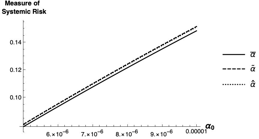
Figure 1: Change in our measure of systemic risk for different estimates of $\alpha_{i}$ ($i=1,2,3$) when varying $\alpha_{0}$.

As expected, our measure of systemic risk increases for larger values of $\alpha_{0}$.

The following corollary related to the market failure probability as $\varepsilon\rightarrow 0$ follows easily from Theorem 3.

Corollary 10.

(Market Failure when $\varepsilon\rightarrow 0$)

$$\lim_{\varepsilon\rightarrow 0}\frac{\mathbb{P}\left(\tau_{1}\in\left(t,t+\varepsilon\right],\tau_{2}\in\left(t,t+\varepsilon\right]|\tau_{1}>t,\tau_{2}>t,\right)}{\varepsilon}=\mathbb{E}\left(\alpha_{0}(X_{t})\right).$$ (12)

Proof.

Note that

$$\mathbb{P} \left(\tau_{1}\in\left(t,t+\varepsilon\right],\tau_{2}\in\left(t,t+\varepsilon\right]|\tau_{1}>t,\tau_{2}>t,\left(X_{u}\right)_{u\leq t+\varepsilon}\right)$$

$$=\frac{\mathbb{P}\left(\tau_{1}\in\left(t,t+\varepsilon\right],\tau_{2}\in\left(t,t+\varepsilon\right]|\left(X_{u}\right)_{u\leq t+\varepsilon}\right)}{\mathbb{P}\left(\tau_{1}>t,\tau_{2}>t|\left(X_{u}\right)_{u\leq t+\varepsilon}\right)}.$$

For the numerator, using Theorem 3 with $K=2$,

$$\mathbb{P}\left(\tau_{1}\in\left(t,t+\varepsilon\right],\tau_{2}\in\left(t,t+\varepsilon\right]|\left(X_{u}\right)_{u\leq t+\varepsilon}\right)=\\ \mathbb{P}\left(\tau_{1}>t,\tau_{2}>t|\left(X_{u}\right)_{u\leq t+\varepsilon}\right)-\mathbb{P}\left(\tau_{1}>t,\tau_{2}>t+\varepsilon|\left(X_{u}\right)_{u\leq t+\varepsilon}\right)\\ -\mathbb{P}\left(\tau_{1}>t+\varepsilon,\tau_{2}>t|\left(X_{u}\right)_{u\leq t+\varepsilon}\right)+\mathbb{P}\left(\tau_{1}>t+\varepsilon,\tau_{2}>t+\varepsilon|\left(X_{u}\right)_{u\leq t+\varepsilon}\right)=\\ \exp\left[-\left(A_{1}+A_{2}+A_{0}\right)\left(t\right)\right]-\exp\left[-A_{1}\left(t\right)-\left(A_{2}+A_{0}\right)\left(t+\varepsilon\right)\right]\\ -\exp\left[-\left(A_{1}+A_{0}\right)\left(t+\varepsilon\right)-A_{2}\left(t\right)\right]+\exp\left[-\left(A_{1}+A_{2}+A_{0}\right)\left(t+\varepsilon\right)\right].$$

Dividing by $\mathbb{P}\left(\tau_{1}>t,\tau_{2}>t|\left(X_{u}\right)_{u\leq t+\varepsilon}\right)=\exp\left[-A_{1}\left(t\right)-A_{2}\left(t\right)-A_{0}\left(t\right)\right]$, we get:

$$\mathbb{P} \left(\tau_{1}\in\left(t,t+\varepsilon\right],\tau_{2}\in\left(t,t+\varepsilon\right]|\tau_{1}>t,\tau_{2}>t,\left(X_{u}\right)_{u\leq t+\varepsilon}\right)=1$$

$$-\exp\left[-\int\limits_{t}^{t+\varepsilon}\left(\alpha_{2}+\alpha_{0}\right)(X_{u})du\right]-\exp\left[-\int\limits_{t}^{t+\varepsilon}\left(\alpha_{1}+\alpha_{0}\right)(X_{u})du\right]$$

$$+\exp\left[-\int\limits_{t}^{t+\varepsilon}\left(\alpha_{1}+\alpha_{2}+\alpha_{0}\right)(X_{u})du\right].$$

Hence, by using L’Hôpital’s rule, we get:

$$\lim_{\varepsilon\rightarrow 0}\frac{\mathbb{P}\left(\tau_{1}\in\left(t,t+\varepsilon\right],\tau_{2}\in\left(t,t+\varepsilon\right]|\tau_{1}>t,\tau_{2}>t,\left(X_{u}\right)_{u\leq t+\varepsilon}\right)}{\varepsilon}=\\ \left(\alpha_{2}+\alpha_{0}\right)\left(X_{t}\right)+\left(\alpha_{1}+\alpha_{0}\right)\left(X_{t}\right)-\left(\alpha_{1}+\alpha_{2}+\alpha_{0}\right)\left(X_{t}\right)=\alpha_{0}(X_{t}).$$

Moreover, given $\mathbb{P}\left(\tau_{1}\in\left(t,t+\varepsilon\right],\tau_{2}\in\left(t,t+\varepsilon\right]|\tau_{1}>t,\tau_{2}>t,\left(X_{u}\right)_{u\leq t+\varepsilon}\right)$ is bounded by 1 and a conditioning argument, we can conclude that

$$\lim_{\varepsilon\rightarrow 0}\frac{\mathbb{P}\left(\tau_{1}\in\left(t,t+\varepsilon\right],\tau_{2}\in\left(t,t+\varepsilon\right]|\tau_{1}>t,\tau_{2}>t,\right)}{\varepsilon}=\mathbb{E}\left(\alpha_{0}(X_{t})\right).$$ (13)

∎

That is, the probability of a market failure due to two banks defaulting over the next time interval $(t,t+\varepsilon]$ with $\varepsilon\approx 0$ is equal to the probability of a market-wide stress event occurring, as noted before.

3.3 Catastrophic Market Failure

It is of interest to determine the probability that all banks will default within a small interval of time. This would be a catastrophic market failure.

Theorem 11.

(Occurrence of all the Default Times)

Let $\tau_{(K)}=max\{\tau_{1},...,\tau_{K}\}$.

$$\mathbb{P}\left(\tau_{(K)}\leq\varepsilon\right)=1+\mathbb{E}\left[e^{-A_{0}\left(\varepsilon\right)}\left(\prod\limits_{i=1}^{K}\left(1-e^{-A_{i}\left(\varepsilon\right)}\right)-1\right)\right].$$ (14)

Proof.

For any $K$, we have

$$\tilde{\mathbb{P}}\left(\tau_{(K)}\leq\varepsilon\right)= \tilde{\mathbb{P}}\left(\tau_{1}\leq\varepsilon,\tau_{2}\leq\varepsilon,\dots,\tau_{K}\leq\varepsilon\right)$$

$$= \tilde{\mathbb{P}}\left(\tau_{1}\leq\varepsilon,\tau_{2}\leq\varepsilon,\dots,\tau_{K}\leq\varepsilon,\eta_{0}>\varepsilon\right)$$

$$+\tilde{\mathbb{P}}\left(\tau_{1}\leq\varepsilon,\tau_{2}\leq\varepsilon,\dots,\tau_{K}\leq\varepsilon,\eta_{0}\leq\varepsilon\right).$$

As $$\tau_{i}=\min\left(\eta_{i},\eta_{0}\right) \left\{\tau_{1}\leq\varepsilon,\tau_{2}\leq\varepsilon,\dots,\tau_{K}\leq\varepsilon,\eta_{0}>\varepsilon\right\} \left\{\eta_{1}\leq\varepsilon,\eta_{2}\leq\varepsilon,\dots,\eta_{K}\leq\varepsilon,\eta_{0}>\varepsilon\right\} \left\{\tau_{1}\leq\varepsilon,\tau_{2}\leq\varepsilon,\dots,\tau_{K}\leq\varepsilon,\eta_{0}\leq\varepsilon\right\} \left\{\eta_{0}\leq\epsilon\right\}$$, the event is equal to and is equal to

$$\tilde{\mathbb{P}}(\tau_{(K)}\leq\varepsilon)= \tilde{\mathbb{P}}\left(\eta_{1}\leq\varepsilon,\eta_{2}\leq\varepsilon,\dots,\eta_{K}\leq\varepsilon,\eta_{0}>\varepsilon\right)+\tilde{\mathbb{P}}\left(\eta_{0}\leq\varepsilon\right).$$

Using the independence of $$\eta_{i}$$

$$\tilde{\mathbb{P}}(\tau_{(K)}\leq\varepsilon)= \tilde{\mathbb{P}}\left(\eta_{0}>\varepsilon\right)\tilde{\mathbb{P}}\left(\eta_{1}\leq\varepsilon\right)\tilde{\mathbb{P}}\left(\eta_{2}\leq\varepsilon\right)\dots\tilde{\mathbb{P}}\left(\eta_{K}\leq\varepsilon\right)+\tilde{\mathbb{P}}\left(\eta_{0}\leq\varepsilon\right)$$

$$= e^{-A_{0}\left(\varepsilon\right)}\left[\prod\limits_{i=1}^{K}\left(1-e^{-A_{i}(\varepsilon)}\right)\right]+1-e^{-A_{0}\left(\varepsilon\right)}$$

$$= 1+e^{-A_{0}\left(\varepsilon\right)}\left[\prod\limits_{i=1}^{K}\left(1-e^{-A_{i}(\varepsilon)}\right)-1\right].$$

The result follows by taking an additional expectation. ∎

Remark 12.

(Catastrophic Market Failure with Identical Distributions)

Let $A_{i}(\varepsilon)$ for $i=1,2,\dots,K$ be the same for all banks and independent of $K$, say $A(\varepsilon)$, implying that the G-SIBs’ default times are identically distributed. Then, $\lim_{K\rightarrow\infty}\prod\limits_{i=1}^{K}\left(1-e^{-A_{i}\left(\varepsilon\right)}\right)=\lim_{K\rightarrow\infty}\left(1-e^{-A\left(\varepsilon\right)}\right)^{K}=0$, which implies that

$$\lim_{K\rightarrow\infty}\mathbb{P}\left(\tau_{(K)}<\varepsilon\right)=1-\mathbb{E}\left(e^{-A_{0}(\varepsilon)}\right)=\mathbb{P}\left(\eta_{0}<\varepsilon\right).$$ (15)

As the number of G-SIBs approaches infinity, the probability of a catastrophic market failure is equal to the probability of a market-wide stress event occurring. This makes sense since, except for the market-wide stress event, the probability of idiosyncratic defaults are independent across G-SIBs.

Corollary 13.

(Catastrophic Market Failure with Constant Default Intensities)

If $\alpha_{i}(X_{t})=\alpha_{i}$ for all $t\geq 0$, all $i=1,2,\dots,K$, and where $\alpha_{i}\in\mathbb{R}^{+}$, then:

$$\mathbb{P}\left(\tau_{(K)}\leq\varepsilon\right)=1+e^{-\alpha_{0}\varepsilon}\left(\prod\limits_{i=1}^{K}\left(1-e^{\alpha_{i}\varepsilon}\right)-1\right).$$ (16)

Remark 14.

(Destructive Competition)

With destructive competition (see Example 1) and assuming that for all $i=1,2,\dots,K$, $\alpha_{i}(X_{t},K)=\ln(K)+b(X_{t})$ and $\varepsilon<1$, then

$$\lim_{K\rightarrow\infty}\mathbb{P}\left(\tau_{(K)}<\varepsilon\right)=\mathbb{P}\left(\eta_{0}<\varepsilon\right).$$ (17)

As documented, under destructive competition, the probability of a catastrophic market failure increases to the indicated limit as the number of GSIBs approaches infinity.

Proof.

(Destructive Competition) Recall that:

$$\mathbb{P}\left(\tau_{(K)}\leq\varepsilon\right)=1-\mathbb{E}\left[e^{-A_{0}\left(\varepsilon\right)}\left(1-\prod\limits_{i=1}^{K}\left(1-e^{-A_{i}\left(\varepsilon,K\right)}\right)\right)\right].$$ (18)

If $\alpha_{i}(X_{t},K)=\ln(K)+b(X_{t})$, then

$$\tilde{\mathbb{P}}\left(\tau_{(K)}\leq\varepsilon\right) =1-e^{-A_{0}\left(\varepsilon\right)}\left(1-\left(1-e^{-A\left(\varepsilon,K\right)}\right)^{K}\right)$$

$$=1-e^{-A_{0}\left(\varepsilon\right)}\left(1-\left(1-e^{-\varepsilon\ln(K)-B(\varepsilon)}\right)^{K}\right)$$

$$=1-e^{-A_{0}\left(\varepsilon\right)}\left(1-\left(1-\frac{e^{-B(\varepsilon)}}{K^{\varepsilon}}\right)^{K}\right)$$

$$\overset{K\rightarrow\infty}{\longrightarrow}1-e^{-A_{0}\left(\varepsilon\right)}.$$ (19)

The results follow by taking an expectation and interchanging limits, which we can do because $\tilde{\mathbb{P}}(\cdot)$ is bounded by 1. ∎

3.4 Bounds on the Market Failure Probability

For some empirical applications, it may be useful to obtain bounds on the market failure probability as in the subsequent theorem.

Theorem 15.

(Bounds on the Market Failure Probability)

$$\mathbb{P}\left(\left|\tau_{i}-\tau_{j}\right|<\varepsilon\text{ for some }(i,j),i\neq j\right)\leq\\ \min\left[\binom{K}{2}-\sum\limits_{i=1}^{K}\sum\limits_{j\neq i}^{K}\mathbb{E}\left(\int_{0}^{\infty}\alpha_{i}(X_{x})e^{-A_{i}(x)-A_{j}(x+\varepsilon)-A_{0}(x+\varepsilon)}dx\right),\right.\\ 1-\mathbb{E}\Biggl{(}\sum_{j\in S(P_{K})}\int\limits_{0}^{\infty}f_{j_{1}}(x_{1})\int\limits_{x_{1}+\varepsilon}^{\infty}f_{j_{2}}(x_{2})\int\limits_{x_{2}+\varepsilon}^{\infty}f_{j_{3}}(x_{3})\dots\int\limits_{x_{K-3}+\varepsilon}^{\infty}f_{j_{K-2}}(x_{K-2})\\ \int\limits_{x_{K-2}+\varepsilon}^{\infty}f_{j_{K-1}}(x_{K-1})\exp\left[-A_{j_{K}}(x_{K-1}+\varepsilon)-A_{0}(x_{K-1}+\varepsilon)\right]\,dx_{K-1}\,dx_{K-2}\dots{\\ }\left.\dots\,dx_{3}\,dx_{2}\,dx_{1}\Biggr{)}\right]$$ (20)

where $S\left(P_{K}\right)$ stands for a subset of $P_{K}$ (Recall $P_{K}$ stands for the set of all possible permutations of $(1,2,\dots,K)$).

$$\mathbb{P}\left(\left|\tau_{i}-\tau_{j}\right|<\varepsilon\text{ for some }(i,j),i\neq j\right)\geq\\ \max\left[1-\mathbb{E}\left(e^{-A_{0}\left((K-1)\varepsilon\right)}\sum\limits_{j\in P_{K}}\exp\left(-\sum\limits_{i=1}^{K-1}A_{j_{i+1}}\left(i\varepsilon\right)\right)\right),\right.\\ \left.1-\min\limits_{i\neq j}\left(\int_{0}^{\infty}\alpha_{i}(x)e^{-A_{i}(x)-(A_{j}+A_{0})(x+\varepsilon)}dx+\int_{0}^{\infty}\alpha_{j}(x)e^{-A_{j}(x)-(A_{i}+A_{0})(x+\varepsilon)}dx\right)\right].$$ (21)

Proof.

Note that by construction $\eta_{0},\eta_{1},\eta_{2},\dots,\eta_{K}$ are mutually independent.

For the first upper bound, note the following:

$$\tilde{\mathbb{P}} \left(\left|\tau_{i}-\tau_{j}\right|<\varepsilon\;for\>some\>(i,j)\in\left(1,...,K\right)\times\left(1,...,K\right),i\neq j\right)$$

$$=\tilde{\mathbb{P}}\left(\bigcup_{i=1}^{K}\bigcup_{j>i}|\tau_{i}-\tau_{j}|\leq\varepsilon\right)\leq\sum\limits_{i=1}^{K}\sum\limits_{j>i}\tilde{\mathbb{P}}\left(|\tau_{i}-\tau_{j}|\leq\varepsilon\right).$$ (22)

For any $i,j$, we have:

$$\tilde{\mathbb{P}}\left(|\tau_{i}-\tau_{j}|\leq\varepsilon\right)=1-\tilde{\mathbb{P}}\left(\tau_{i}-\tau_{j}>\varepsilon,\tau_{i}>\tau_{j}\right)-\tilde{\mathbb{P}}\left(\tau_{j}-\tau_{i}>\varepsilon,\tau_{j}>\tau_{i}\right).$$

Let us focus on $\tilde{\mathbb{P}}\left(\tau_{i}-\tau_{j}>\varepsilon,\tau_{i}>\tau_{j}\right)$ and note that in the next equality we do not consider the event $\{\eta_{i}>\eta_{j}>\eta_{0}\}$ because it implies $\tau_{i}=\tau_{j}$ and so it is impossible to have $\tau_{i}-\tau_{j}>\varepsilon$

$$\tilde{\mathbb{P}} \left(\tau_{i}-\tau_{j}>\varepsilon,\tau_{i}>\tau_{j}\right)=\tilde{\mathbb{P}}\left(\tau_{i}-\tau_{j}>\varepsilon,\eta_{0}>\eta_{i}>\eta_{j}\right)$$

$$+\tilde{\mathbb{P}}\left(\tau_{i}-\tau_{j}>\varepsilon,\eta_{i}>\eta_{0}>\eta_{j}\right)=\int\limits_{0}^{\infty}\int\limits_{y+\varepsilon}^{\infty}\int\limits_{x}^{\infty}f_{0}(z)f_{i}(x)f_{j}(y)\,dz\,dx\,dy$$

$$+\int\limits_{0}^{\infty}\int\limits_{y+\varepsilon}^{\infty}\int\limits_{z}^{\infty}f_{i}(x)f_{0}(z)f_{j}(y)\,dx\,dz\,dy=\int\limits_{0}^{\infty}f_{j}(y)\int\limits_{y+\varepsilon}^{\infty}\alpha_{i}(X_{x})e^{-A_{i}(x)-A_{0}(x)}\,dx\,dy$$

$$+\int\limits_{0}^{\infty}f_{j}(y)\int\limits_{y+\varepsilon}^{\infty}\alpha_{0}(X_{z})e^{-A_{i}(z)-A_{0}(z)}\,dz\,dy$$

$$=\int\limits_{0}^{\infty}f_{j}(y)\int\limits_{y+\varepsilon}^{\infty}\left[\alpha_{i}(X_{x})+\alpha_{0}(X_{x})\right]e^{-A_{i}(x)-A_{0}(x)}\,dx\,dy$$

$$=\int\limits_{0}^{\infty}\alpha_{j}(y)e^{-A_{j}(y)-A_{i}(y+\varepsilon)-A_{0}(y+\varepsilon)}\,dy.$$

$\tilde{\mathbb{P}}\left(\tau_{i}-\tau_{j}>\varepsilon,\tau_{j}>\tau_{i}\right)$ follows by an analogous argument:

$$\tilde{\mathbb{P}}\left(\tau_{i}-\tau_{j}>\varepsilon,\tau_{j}>\tau_{i}\right)=\int\limits_{0}^{\infty}\alpha_{i}(y)e^{-A_{i}(y)-A_{j}(y+\varepsilon)-A_{0}(y+\varepsilon)}\,dy.$$

Joining these 2 probabilities, we get:

$$\tilde{\mathbb{P}}\left(|\tau_{i}-\tau_{j}|\leq\varepsilon\right)=1-\int\limits_{0}^{\infty}\alpha_{j}(y)e^{-A_{j}(y)-A_{i}(y+\varepsilon)-A_{0}(y+\varepsilon)}dy\\ -\int\limits_{0}^{\infty}\alpha_{i}(y)e^{-A_{i}(y)-A_{j}(y+\varepsilon)-A_{0}(y+\varepsilon)}dy.$$

Using this along with (3.4), we get:

$$\tilde{\mathbb{P}}\left(\left|\tau_{i}-\tau_{j}\right|<\varepsilon\;for\>some\>(i,j)\in\left(1,...,K\right)\times\left(1,...,K\right),i\neq j\right)\\ \leq\sum\limits_{i=1}^{K}\sum\limits_{j>i}\left[1-\int\limits_{0}^{\infty}\alpha_{j}(y)e^{-A_{j}(y)-A_{i}(y+\varepsilon)-A_{0}(y+\varepsilon)}dy\right.\\ \left.-\int\limits_{0}^{\infty}\alpha_{i}(y)e^{-A_{i}(y)-A_{j}(y+\varepsilon)-A_{0}(y+\varepsilon)}dy\right]\\ =\binom{K}{2}-\sum\limits_{i=1}^{K}\sum\limits_{j\neq i}^{K}\int\limits_{0}^{\infty}\alpha_{i}(y)e^{-A_{i}(y)-A_{j}(y+\varepsilon)-A_{0}(y+\varepsilon)}dy.$$

Finally, the desired upper bound follows by taking an additional expectation.

The second upper bound is natural as we are taking a sum over a smaller set.

For the first lower bound, it suffices to bound

$$\mathbb{P}\left(|\tau_{i}-\tau_{j}|>\varepsilon\text{ for all }(i,j),i\neq j\right)$$

from above. This is because:

$$\mathbb{P}\left(\left|\tau_{i}-\tau_{j}\right|<\varepsilon\text{ for some }(i,j),i\neq j\right)=1-\mathbb{P}\left(|\tau_{i}-\tau_{j}|>\varepsilon\text{ for all }(i,j),i\neq j\right).$$

From Theorem 6, we know that,

$$\tilde{\mathbb{P}}\left(|\tau_{i}-\tau_{j}|>\varepsilon\text{ for all }(i,j),i\neq j\right)=\sum_{j\in P_{K}}\int\limits_{0}^{\infty}f_{j_{1}}(x_{1})\int\limits_{x_{1}+\varepsilon}^{\infty}f_{j_{2}}(x_{2})\\ \int\limits_{x_{2}+\varepsilon}^{\infty}f_{j_{3}}(x_{3})\dots\int\limits_{x_{K-3}+\varepsilon}^{\infty}f_{j_{K-2}}(x_{K-2})\int\limits_{x_{K-2}+\varepsilon}^{\infty}f_{j_{K-1}}(x_{K-1})\exp\left[-A_{j_{K}}(x_{K-1}+\varepsilon)\right.\\ \left.-A_{0}(x_{K-1}+\varepsilon)\right]\,dx_{K-1}\,dx_{K-2}\dots\,dx_{3}\,dx_{2}\,dx_{1}.$$

As $x_{K-1}\geq x_{K-2}+\varepsilon$ in the innermost integral in one of the terms of the previous sum, then $e^{-\left(A_{j_{K}}+A_{0}\right)(x_{K-1}+\varepsilon)}\leq e^{-\left(A_{j_{K}}+A_{0}\right)(x_{K-2}+2\varepsilon)}$ and hence:

$$\int\limits_{0}^{\infty}f_{j_{1}}(x_{1})\int\limits_{x_{1}+\varepsilon}^{\infty}f_{j_{2}}(x_{2})\dots{\\ }\dots\int\limits_{x_{K-2}+\varepsilon}^{\infty}f_{j_{K-1}}(x_{K-1})e^{-\left(A_{j_{K}}+A_{0}\right)(x_{K-1}+\varepsilon)}dx_{K-1}\dots\,dx_{1}\\ \leq\int\limits_{0}^{\infty}f_{j_{1}}(x_{1})\int\limits_{x_{1}+\varepsilon}^{\infty}f_{j_{2}}(x_{2})\dots e^{-\left(A_{j_{K}}+A_{0}\right)(x_{K-2}+2\varepsilon)}\\ \int\limits_{x_{K-2}+\varepsilon}^{\infty}f_{j_{K-1}}(x_{K-1})\,dx_{K-1}\dots\,dx_{2}\,dx_{1}\\ =\int\limits_{0}^{\infty}f_{j_{1}}(x_{1})\int\limits_{x_{1}+\varepsilon}^{\infty}f_{j_{2}}(x_{2})\dots{\\ }\dots\int\limits_{x_{K-3}+\varepsilon}^{\infty}f_{j_{K-2}}(x_{K-2})e^{-\left(A_{j_{K}}+A_{0}\right)(x_{K-2}+2\varepsilon)-A_{j_{K-1}}(x_{K-2}+\varepsilon)}\,dx_{K-2}\dots\,dx_{2}\,dx_{1}.$$

As $x_{K-2}\geq x_{K-3}+\varepsilon$ in the innermost integral, we have

$$e^{-\left(A_{j_{K}}+A_{0}\right)(x_{K-2}+2\varepsilon)-A_{j_{K-1}}(x_{K-2}+\varepsilon)}\leq e^{-\left(A_{j_{K}}+A_{0}\right)(x_{K-3}+3\varepsilon)-A_{j_{K-1}}(x_{K-3}+2\varepsilon)}.$$

Then, we solve the integral with respect to $x_{K-2}$. We keep going in a similar fashion to conclude that:

$$\int\limits_{0}^{\infty}f_{j_{1}}(x_{1})\int\limits_{x_{1}+\varepsilon}^{\infty}f_{j_{2}}(x_{2})\dots{\\ }\dots\int\limits_{x_{K-2}+\varepsilon}^{\infty}f_{j_{K-1}}(x_{K-1})e^{-\left(A_{j_{K}}+A_{0}\right)(x_{K-1}+\varepsilon)}\,dx_{K-1}\dots\,dx_{2}\,dx_{1}\\ \leq\exp\left[-\left(A_{j_{K}}+A_{0}\right)\left((K-1)\varepsilon\right)-A_{j_{K-1}}\left((K-2)\varepsilon\right)-\dots\right.\\ \left.\dots-A_{j_{3}}(2\varepsilon)-A_{j_{2}}(\varepsilon)\right]=\exp\left[-A_{0}\left((K-1)\varepsilon\right)-\sum\limits_{i=1}^{K-1}A_{j_{i+1}}\left(i\varepsilon\right)\right].$$

Then we take the sum over all possible permutations $P_{K}$ to get:

$$\tilde{\mathbb{P}}\left(|\tau_{i}-\tau_{j}|>\varepsilon\text{ for all }(i,j),i\neq j\right)\leq\\ \sum_{j\in P_{K}}\exp\left[-A_{0}\left((K-1)\varepsilon\right)-\sum\limits_{i=1}^{K-1}A_{j_{i+1}}\left(i\varepsilon\right)\right].$$

Recall that the sub index $j$ in the sum stands for any of the possible permutations. This is $j=\left(j_{1}=\sigma(1),j_{2}=\sigma(2),\dots,j_{K}=\sigma(K)\right)$ Using the complement of the previous probability, we have

$$\tilde{\mathbb{P}}\left(\left|\tau_{i}-\tau_{j}\right|<\varepsilon\text{ for some }(i,j),i\neq j\right)\geq\\ 1-e^{-A_{0}\left((K-1)\varepsilon\right)}\sum\limits_{j\in P_{K}}\exp\left(-\sum\limits_{i=1}^{K-1}A_{j_{i+1}}\left(i\varepsilon\right)\right).$$

The desired lower bound follows by taking an additional expectation.

For the second lower bound, note that:

$$\mathbb{P}\left(|\tau_{i}-\tau_{j}|>\varepsilon\text{ for all }(i,j),i\neq j\right)=\\ \mathbb{P}\left(\bigcap\limits_{i=1}^{K}\bigcap\limits_{j\neq i}^{K}|\tau_{i}-\tau_{j}|>\varepsilon\right)\leq\min\limits_{i\neq j}\mathbb{P}\left(|\tau_{i}-\tau_{j}|>\varepsilon\right)\\ =\min\limits_{i\neq j}\left[\int_{0}^{\infty}\alpha_{i}(x)e^{-A_{i}(x)-(A_{j}+A_{0})(x+\varepsilon)}dx+\int_{0}^{\infty}\alpha_{j}(x)e^{-A_{j}(x)-(A_{i}+A_{0})(x+\varepsilon)}dx\right].$$ (23)

And then, use the following:

$$\mathbb{P}\left(\left|\tau_{i}-\tau_{j}\right|<\varepsilon\text{ for some }(i,j),i\neq j\right)=1-\mathbb{P}\left(|\tau_{i}-\tau_{j}|>\varepsilon\text{ for all }(i,j),i\neq j\right).$$

∎

Corollary 16.

(Constant Default Intensities)

If $\alpha_{i}(X_{t})=\alpha_{i}$ for all $t\geq 0$, all $i=1,2,\dots,K$, and where $\alpha_{i}\in\mathbb{R}^{+}$, then:

$$\mathbb{P}\left(\left|\tau_{i}-\tau_{j}\right|<\varepsilon\text{ for some }(i,j),i\neq j\right)\leq\\ \min\left[\binom{K}{2}-e^{-\alpha_{o}\varepsilon}\sum\limits_{i=1}^{K}\alpha_{i}\sum\limits_{j\neq i}^{K}e^{\alpha_{j}\varepsilon}\left(\frac{1}{\alpha_{i}+\alpha_{j}+\alpha_{0}}\right),\right.\\ \left.1-\sum_{j\in S\left(P_{K}\right)}\prod\limits_{i=1}^{K-1}\left(\frac{\alpha_{j_{i}}}{\alpha_{0}+\sum\limits_{k=i}^{K}\alpha_{j_{k}}}e^{-\varepsilon\left(\alpha_{0}+\sum\limits_{k=i+1}^{K}\alpha_{j_{k}}\right)}\right)\right].$$ (24)

$$\mathbb{P}\left(\left|\tau_{i}-\tau_{j}\right|<\varepsilon\text{ for some }(i,j),i\neq j\right)\geq\\ \max\left[1-e^{\alpha_{0}\varepsilon\left(K-1\right)}\sum\limits_{j\in P_{K}}\exp\left(-\varepsilon\sum\limits_{i=1}^{K-1}i\alpha_{j_{i+1}}\right),\right.\\ \left.1-\min_{i\neq j}\left(e^{-\varepsilon\alpha_{0}}\frac{1}{\alpha_{i}+\alpha_{j}+\alpha_{0}}\left(\alpha_{i}e^{-\varepsilon\alpha_{j}}+\alpha_{j}e^{-\varepsilon\alpha_{i}}\right)\right)\right].$$ (25)

4 Comparative Statics

This section explores how the market failure probability changes when the initial conditions in the economy change. We consider both changing the number of G-SIBs and the initial state of the economy.

4.1 The Number of G-SIBs

For regulatory purposes, it is important to understand how the probability of a market failure changes with the inclusion of another G-SIB. This relates to macro-prudential policy regarding whether the number of banks in the economy being “too large to fail” or designated as G-SIBs should be reduced (by breaking them up into smaller institutions) to decrease the market failure probability (see Berndt et al., (2021), Schich & Toader, (2017) for issues related to G-SIBs designation).

Computing the market failure probability for $K$ banks versus $K+1$ banks in Theorem 6 and taking the difference yields the marginal impact of adding another G-SIB to the economy. It is easy to show that this probability increases as more G-SIBs enter the market.

Theorem 17.

(Increasing the Number of G-SIBs)

$$\mathbb{P}\left(\left|\tau_{i}-\tau_{j}\right|<\varepsilon\;for\>some\>(i,j)\in\left(1,\dots,K\right)\times\left(1,\dots,K\right),i\neq j\right)<\\ \mathbb{P}\left(\left|\tau_{i}-\tau_{j}\right|<\varepsilon\;for\>some\>(i,j)\in\left(1,\dots,K+1\right)\times\left(1,\dots,K+1\right),i\neq j\right)$$ (26)

provided that $\alpha_{i}(\cdot)$ for $i=0,1,2,\dots,K$ and the underlying process, i.e., $(X_{t})_{t\geq 0}$ remain fixed.

Proof.

Let

$$A :=\{\left|\tau_{i}-\tau_{j}\right|<\varepsilon\;for\>some\>(i,j)\in\left(1,...,K\right)^{2},i\neq j\}$$ (27)

$$B :=\{\left|\tau_{i}-\tau_{j}\right|<\varepsilon\;for\>some\>(i,j)\in\left(1,\dots,K,K+1\right)^{2},i\neq j\}.$$ (28)

Note that the event $B$ can be decomposed in the following way:

$$B=A\cup\{\left|\tau_{K+1}-\tau_{j}\right|<\varepsilon\;for\>some\>j\in\left(1,...,K\right)\}.$$ (29)

It is clear that $A\subsetneq B$ and hence the result follows . ∎

This result suggests that as the number of G-SIBs goes to infinity, the market failure probability converges to one, as the following theorem documents.

Theorem 18.

(Limit as $K\rightarrow\infty$)

$$\lim_{K\rightarrow\infty}\mathbb{P}\left(\left|\tau_{i}-\tau_{j}\right|<\varepsilon\;for\>some\>(i,j)\in\left(1,...,K\right)\times\left(1,...,K\right),i\neq j\right)=1.$$ (30)

Proof.

Similar to the proof of Theorem 3, for $k=1,2,\dots,K$, let $\tau_{(k)}$ and $\eta_{(k)}$ be the $k^{th}$ order statistic of $\left(\tau_{1},\tau_{2},\dots,\tau_{K}\right)$ and $\left(\eta_{1},\eta_{2},\dots,\eta_{K}\right)$ respectively. For example, $\tau_{(1)}=\min\left(\tau_{1},\tau_{2},\dots,\tau_{K}\right)$, $\eta_{(1)}=\min\left(\eta_{1},\eta_{2},\dots,\eta_{K}\right)$, $\tau_{(K)}=\max\left(\tau_{1},\tau_{2},\dots,\tau_{K}\right)$ and $\eta_{(K)}=\max\left(\eta_{1},\eta_{2},\dots,\eta_{K}\right)$.

The complement of the event $\left\{\left|\tau_{i}-\tau_{j}\right|<\varepsilon\;\mathrm{for\>some}\>(i,j),\>i\neq j\right\}$ is equal to the event $\left\{\left|\tau_{i}-\tau_{j}\right|\geq\varepsilon\;\mathrm{for\>all}\>(i,j),\>i\neq j\right\}$. Then, we get:

$$\tilde{\mathbb{P}}\left(\left|\tau_{i}-\tau_{j}\right|\geq\varepsilon\;\mathrm{for\>all}\>(i,j),\>i\neq j\right)=\\ \tilde{\mathbb{P}}\left(\left|\tau_{i}-\tau_{j}\right|\geq\varepsilon\;\mathrm{for\>all}\>(i,j),\>i\neq j,\eta_{0}\geq\eta_{(K)}\right)\\ +\tilde{\mathbb{P}}\left(\left|\tau_{i}-\tau_{j}\right|\geq\varepsilon\;\mathrm{for\>all}\>(i,j),\>i\neq j,\eta_{(k-1)}\leq\eta_{0}<\eta_{(K)}\right)\\ +\tilde{\mathbb{P}}\left(\left|\tau_{i}-\tau_{j}\right|\geq\varepsilon\;\mathrm{for\>all}\>(i,j),\>i\neq j,\eta_{0}<\eta_{(K-1)}\right).$$ (31)

If $\eta_{0}<\eta_{(K-1)}$, then at least there exists one pair of $(i,j)$, $i\neq j$ such that $\tau_{i}=\tau_{j}=\eta_{0}$ and hence, $\tilde{\mathbb{P}}\left(\left|\tau_{i}-\tau_{j}\right|\geq\varepsilon\;\mathrm{for\>all}\>(i,j),\>i\neq j,\eta_{0}<\eta_{(K-1)}\right)=0$.

If $\left|\tau_{i}-\tau_{j}\right|\geq\varepsilon\;\mathrm{for\>all}\>(i,j),\>i\neq j$, then $\tau_{(2)}\geq\tau_{(1)}+\varepsilon$, $\tau_{(3)}\geq\tau_{(2)}+\varepsilon,\dots,\tau_{(K)}\geq\tau_{(K-1)}+\varepsilon$, which implies $\tau_{(K)}\geq\tau_{(1)}+\left(K-1\right)\varepsilon$. Moreover, on the event $\{\eta_{0}\geq\eta_{(K)}\}$, we have that $\tau_{(K)}=\eta_{(K)}$ and $\tau_{(1)}=\eta_{(1)}$. Hence,

$$\tilde{\mathbb{P}}\left(\left|\tau_{i}-\tau_{j}\right|\geq\varepsilon\;\mathrm{for\>all}\>(i,j),\>i\neq j,\eta_{0}\geq\eta_{(K)}\right)\\ \leq\tilde{\mathbb{P}}\left(\tau_{(K)}\geq\tau_{(1)}+\left(K-1\right)\varepsilon,\eta_{0}\geq\eta_{(K)}\right)\\ =\tilde{\mathbb{P}}\left(\eta_{(K)}\geq\eta_{(1)}+\left(K-1\right)\varepsilon,\eta_{0}\geq\eta_{(K)}\right)\\ =\tilde{\mathbb{P}}\left(\eta_{(1)}+\left(K-1\right)\varepsilon\leq\eta_{(K)}\leq\eta_{0}\right)\\ \leq\tilde{\mathbb{P}}\left(\eta_{(1)}+\left(K-1\right)\varepsilon\leq\eta_{0}\right).$$ (32)

$$\tilde{\mathbb{P}}\left(\left|\tau_{i}-\tau_{j}\right|\geq\varepsilon\;\mathrm{for\>all}\>(i,j),\>i\neq j,\eta_{0}\geq\eta_{(K)}\right)\\ \leq\tilde{\mathbb{P}}\left(\tau_{(K)}\geq\tau_{(1)}+\left(K-1\right)\varepsilon,\eta_{0}\geq\eta_{(K)}\right)\\ =\tilde{\mathbb{P}}\left(\eta_{(K)}\geq\eta_{(1)}+\left(K-1\right)\varepsilon,\eta_{0}\geq\eta_{(K)}\right)\\ =\tilde{\mathbb{P}}\left(\eta_{(1)}+\left(K-1\right)\varepsilon\leq\eta_{(K)}\leq\eta_{0}\right)\\ \leq\tilde{\mathbb{P}}\left(\eta_{(1)}+\left(K-1\right)\varepsilon\leq\eta_{0}\right).$$ (33)

When taking the limit $K\rightarrow\infty$, as $\eta_{i}$ for $i=0,1,\dots,K$ under $\tilde{\mathbb{P}}$, is a.s. finite, we get

$$\lim_{K\rightarrow\infty}\tilde{\mathbb{P}}\left(\left|\tau_{i}-\tau_{j}\right|\geq\varepsilon\;\mathrm{for\>all}\>(i,j),\>i\neq j,\eta_{0}\geq\eta_{(K)}\right)\\ \leq\lim_{K\rightarrow\infty}\tilde{\mathbb{P}}\left(\eta_{(1)}+\left(K-1\right)\varepsilon\leq\eta_{0}\right)=0.$$ (34)

Now, on the event $\{\eta_{(k-1)}\leq\eta_{0}<\eta_{(K)}\}$, we have that $\tau_{(K)}=\eta_{0}$ and $\tau_{(1)}=\eta_{(1)}$. By a similar reasoning as above,

$$\tilde{\mathbb{P}}\left(\left|\tau_{i}-\tau_{j}\right|\geq\varepsilon\;\mathrm{for\>all}\>(i,j),\>i\neq j,\eta_{(k-1)}\leq\eta_{0}<\eta_{(K)}\right)\\ \leq\tilde{\mathbb{P}}\left(\tau_{(K)}\geq\tau_{(1)}+\left(K-1\right)\varepsilon,\eta_{(k-1)}\leq\eta_{0}<\eta_{(K)}\right)\\ =\tilde{\mathbb{P}}\left(\eta_{0}\geq\eta_{(1)}+\left(K-1\right)\varepsilon,\eta_{(k-1)}\leq\eta_{0}<\eta_{(K)}\right)\\ \leq\tilde{\mathbb{P}}\left(\eta_{(1)}+\left(K-1\right)\varepsilon\leq\eta_{0}\right)\overset{K\rightarrow\infty}{\longrightarrow}0.$$ (35)

The result follows after taking an expectation. The interchange in the expectation and limit as $K\rightarrow\infty$ is justified as $\tilde{\mathbb{P}}\left(\left|\tau_{i}-\tau_{j}\right|\geq\varepsilon\;\mathrm{for\>all}\>(i,j),\>i\neq j\right)$ is bounded by 1. ∎

Consequently, the number of G-SIBs in the economy needs to be restricted by regulators to ensure that the probability of a market failure is at an acceptable level. If the probability of a market failure as implied by the number of existing G-SIBs is too high, then Theorem 6 enables the regulators to select the number of G-SIBs such that the market failure probability is below some given threshold. This implies, of course, that the excess G-SIBs must be broken-up into smaller banks.

Instead of breaking-up the G-SIBs, regulators can alternatively control the probability of a market failure by requiring the existing G-SIBs to change their asset/liability structures. This tool is discussed in the next section.

4.2 Changing the State of the Economy and Banks’ Balance Sheets

This section explores the impact of changing the state of economy vector $X_{r}$ on the market failure probability. The idea, of course, is that some of the inputs are under the control of the regulators, e.g. required capital of a G-SIB. We investigate the impact of changes in the initial conditions on the market failure probability. To facilitate the exposition, let $X_{r}=(x_{1}(r),...,x_{d}(r))$, so that $\alpha_{i}(X_{r})=\alpha_{i}(x_{1}(r),...,x_{d}(r))$.

We redefine the default time for the $i^{th}$ G-SIB due to idiosyncratic events and the first time that a market-wide stress event occurs in the following way:

$$\eta_{i} :=\inf\left\{s:\alpha_{i}\left(X_{0}\right)+A_{i}(s)\geq Z_{i}\right\}\text{ for }i=1,\dots,K$$

$$\eta_{0} :=\inf\left\{s:\alpha_{0}\left(X_{0}\right)+A_{0}(s)\geq Z_{0}\right\}.$$

Just as before, the default time of the $i^{th}$ G-SIB is

$$\tau_{i}=\min\left(\eta_{0},\eta_{i}\right).$$

Then, it is easy to check that

$$\mathbb{P}\left(\eta_{i}>t|\left(X_{u}\right)_{0\leq u\leq t}\right) =\exp\left(-\alpha_{i}\left(X_{0}\right)-A_{i}(t)\right)$$

$$\mathbb{P}\left(\tau_{i}>t|\left(X_{u}\right)_{0\leq u\leq t}\right) =\exp\left(-\alpha_{i}\left(X_{0}\right)-\alpha_{0}\left(X_{0}\right)-A_{i}(t)-A_{0}(t)\right).$$

To ensure that the probability distributions of $\eta_{i}$ and $\tau_{i}$ are correctly defined, we assign a positive probability to the event $\left\{\eta_{i}=0\right\}$ such that

$$\mathbb{P}\left(\eta_{i}=0|X_{0}\right)=1-\exp\left(-\alpha_{i}\left(X_{0}\right)\right).$$

This implies that

$$\mathbb{P}\left(\tau_{i}=0|X_{0}\right)=1-\exp\left(-\alpha_{i}\left(X_{0}\right)-\alpha_{0}\left(X_{0}\right)\right).$$

The interpretation is that there is a positive probability of an “instantaneous” default at $t=0$. Under these modifications, we have the following result.

Theorem 19.

(Comparative Statics)

$$\frac{\partial}{\partial x_{\ell}(0)}\mathbb{P}\left(\left|\tau_{i}-\tau_{j}\right|<\varepsilon\text{ for some }(i,j)\in\left(1,...,K\right)\times\left(1,\dots,K\right),{i\neq j}\right)=\\ \mathbb{E}\left[\left(\sum\limits_{i=0}^{K}\frac{\partial\alpha_{i}(X_{0})}{\partial x_{\ell}(0)}\right)\tilde{\mathbb{P}}\left(\left|\tau_{i}-\tau_{j}\right|\geq\varepsilon\text{ for all }(i,j),{i\neq j}\right)\right]=\\ \mathbb{E}\Biggl{[}\left(\sum\limits_{i=0}^{K}\frac{\partial\alpha_{i}(X_{0})}{\partial x_{\ell}(0)}\exp\left(-\sum\limits_{i=0}^{K}\alpha_{i}(X_{0})\right)\right)\sum_{j\in P_{K}}\int\limits_{0}^{\infty}\hat{f}_{j_{1}}(x_{1})\int\limits_{x_{1}+\varepsilon}^{\infty}\hat{f}_{j_{2}}(x_{2})\\ \int\limits_{x_{2}+\varepsilon}^{\infty}\hat{f}_{j_{3}}(x_{3})\dots\int\limits_{x_{K-2}+\varepsilon}^{\infty}\hat{f}_{j_{K-1}}(x_{K-1})\exp\left[-A_{j_{K}}(x_{K-1}+\varepsilon)-A_{0}(x_{K-1}+\varepsilon)\right]\\ \,dx_{K-1}\dots\,dx_{3}\,dx_{2}\,dx_{1}\Biggr{]}$$ (36)

where $\hat{f}_{j_{k}}(x):={\alpha_{j_{k}}(X_{x})}\exp\left[-A_{j_{k}}(x)\right]$. The derivative is taken with respect to the $\ell$ component of the $\mathbb{R}^{d}$ vector $X$ at time $t=0$, i.e., we are analyzing the market failure probability when changing the initial state of the $\ell$ component of the economy vector.

Proof.

First note that

$$\frac{\partial}{\partial x_{\ell}(0)}\mathbb{P}\left(\left|\tau_{i}-\tau_{j}\right|<\varepsilon\text{ for some }(i,j),i\neq j\right)=\\ \frac{\partial}{\partial x_{\ell}(0)}\mathbb{E}\left[\tilde{\mathbb{P}}\left(\left|\tau_{i}-\tau_{j}\right|<\varepsilon\text{ for some }(i,j),i\neq j\right)\right].$$

As $\tilde{\mathbb{P}}\left(\left|\tau_{i}-\tau_{j}\right|<\varepsilon\text{ for some }(i,j),i\neq j\right)\leq 1$, we can interchange expectation and derivative and so, it suffices to find

$$\frac{\partial}{\partial x_{\ell}(0)}\tilde{\mathbb{P}}\left(\left|\tau_{i}-\tau_{j}\right|<\varepsilon\text{ for some }(i,j),i\neq j\right)$$

and then take an expectation.

Now, with the change of definition of $\eta_{i}$ and $\eta_{0}$, by a similar fashion as in Theorem 6, we get that

$$\tilde{\mathbb{P}}\left(\left|\tau_{i}-\tau_{j}\right|<\varepsilon\text{ for some }(i,j),i\neq j\right)=\\ 1-\tilde{\mathbb{P}}\left(\left|\tau_{i}-\tau_{j}\right|\geq\varepsilon\text{ for all }(i,j),{i\neq j}\right)=\\ 1-\exp\left(-\sum\limits_{i=0}^{K}\alpha_{i}(X_{0})\right)\sum_{j\in P_{K}}\int\limits_{0}^{\infty}\hat{f}_{j_{1}}(x_{1})\int\limits_{x_{1}+\varepsilon}^{\infty}\hat{f}_{j_{2}}(x_{2})\int\limits_{x_{2}+\varepsilon}^{\infty}\hat{f}_{j_{3}}(x_{3})\dots{\\ }\int\limits_{x_{K-2}+\varepsilon}^{\infty}\hat{f}_{j_{K-1}}(x_{K-1})\exp\left[-A_{j_{K}}(x_{K-1}+\varepsilon)-A_{0}(x_{K-1}+\varepsilon)\right]\,dx_{K-1}\dots\,dx_{1}.$$

Differentiating the previous equation with respect to $x_{\ell}(0)$, we obtain

$$\frac{\partial}{\partial x_{\ell}(0)}\tilde{\mathbb{P}}\left(\left|\tau_{i}-\tau_{j}\right|<\varepsilon\text{ for some }(i,j),i\neq j\right)\\ =-\frac{\partial}{\partial x_{\ell}(0)}\tilde{\mathbb{P}}\left(\left|\tau_{i}-\tau_{j}\right|\geq\varepsilon\text{ for all }(i,j),{i\neq j}\right)\\ =\left(\sum\limits_{i=0}^{K}\frac{\partial\alpha_{i}(X_{0})}{\partial x_{\ell}(0)}\right)\tilde{\mathbb{P}}\left(\left|\tau_{i}-\tau_{j}\right|\geq\varepsilon\text{ for all }(i,j),{i\neq j}\right)\\ =\left(\sum\limits_{i=0}^{K}\frac{\partial\alpha_{i}(X_{0})}{\partial x_{\ell}(0)}\exp\left(-\sum\limits_{i=0}^{K}\alpha_{i}(X_{0})\right)\right)\sum_{j\in P_{K}}\int\limits_{0}^{\infty}\hat{f}_{j_{1}}(x_{1})\int\limits_{x_{1}+\varepsilon}^{\infty}\hat{f}_{j_{2}}(x_{2})\dots{\\ }\int\limits_{x_{K-2}+\varepsilon}^{\infty}\hat{f}_{j_{K-1}}(x_{K-1})\exp\left[-A_{j_{K}}(x_{K-1}+\varepsilon)-A_{0}(x_{K-1}+\varepsilon)\right]\,dx_{K-1}\dots\,dx_{1}.$$

∎

Given estimates of the relevant intensities, these partial derivatives are easily computed and they provide the information that regulators can use to determine the impact of their regulatory restrictions on the probability of a market failure.

Remark 20.

(Linear Approximation)

For some simpler calculations, if $\alpha_{i}(X_{r})=\sum_{j=1}^{d}\beta_{ij}x_{j}(r)$ for $\beta_{ij}\in\mathbb{R}^{+}$ and $x_{j}(r)>0$ for $j=1,\dots,d$ and all $r>0$, then

$$\frac{\partial}{\partial x_{\ell}(0)}\mathbb{P}\left(\left|\tau_{i}-\tau_{j}\right|<\varepsilon\text{ for some }(i,j)\in\left(1,...,K\right)\times\left(1,\dots,K\right),{i\neq j}\right)=\\ \left(\sum\limits_{i=0}^{K}\beta_{i\ell}\right)\mathbb{P}\left(\left|\tau_{i}-\tau_{j}\right|\geq\varepsilon\text{ for all }(i,j),{i\neq j}\right).$$ (37)

References

- Acemoglu et al., (2015) Acemoglu, D., Ozdaglar, A., & Tahbaz-Salehi, A. 2015. Systemic Risk and Stability in Financial Networks. American Economic Review, 105(2), 564–608.
- Acharya et al., (2009) Acharya, V., Pedersen, L., Philippon, T., & Richardson, M. 2009. Regulating systemic risk. Chap. 13 of: Acharya, V., & Richardson, M. (eds), Restoring Financial Stability: How to Repair a Failed System. John Wiley and Sons.
- Allen & Carletti, (2013) Allen, F., & Carletti, E. 2013. What Is Systemic Risk? Journal of Money, Credit and Banking, 45(s1), 121–127.
- Bank for International Settlements, (2014) Bank for International Settlements. 2014. The G-SIB assessment methodology - score calculation. Basel Commitee on Banking Supervision, November.
- Berndt et al., (2021) Berndt, A., Duffie, D., & Zhu, Y. 2021. The Decline of Too Big to Fail. Working paper, Stanford University.
- Bielecki & Rutkowski, (2003) Bielecki, T., & Rutkowski, M. 2003. Dependent Defaults and Credit Migrations. Applicationes Mathematicae, 30(2), 121–145.
- Bielecki et al., (2013) Bielecki, T., Cousin, A., Crépey, S., & Herbertsson, A. 2013. In search of a grand unifying theory. Creditflux Newsletter Analysis, July, 20–21.
- Bisias et al., (2012) Bisias, D., Flood, M., Lo, A., & Valavanis, S. 2012. A Survey of Systemic Risk Analytics. Annual Review of Financial Economics, 4(1), 255–296.
- Brigo et al., (2007a) Brigo, D., Pallavicini, A., & Torresetti, R. 2007a. Calibration of CDO Tranches with the Dynamical Generalized-Poisson Loss Model. Available at SSRN.
- Brigo et al., (2007b) Brigo, D., Pallavicini, A., & Torresetti, R. 2007b. Default correlation, cluster dynamics and single names: The GPCL dynamical loss model. Available at arXiv.
- Campbell et al., (2008) Campbell, J. Y., Hilscher, J., & Szilagyi, J. 2008. In Search of Distress Risk. The Journal of Finance, 63(6), 2899–2939.
- Chava & Jarrow, (2004) Chava, S., & Jarrow, R. 2004. Bankruptcy prediction with industry effects. Review of Finance, 8(4), 537–569.
- Coculescu, (2022) Coculescu, D. 2022. A default system with overspilling contagion. Available at arXiv.
- Crouhy et al., (2008) Crouhy, M., Jarrow, R., & Turnbull, S. 2008. The subprime credit crisis of 2007. Journal of Derivatives, Fall, 81–110.
- Duffie et al., (2003) Duffie, D., Jarrow, R., Purnanandam, A., & Yang, M. 2003. Market Pricing of Deposit Insurance. Journal of Financial Services Research, 24(2), 93–119.
- El Karoui et al., (2017) El Karoui, N., Jeanblanc, M., & Jiao, Y. 2017. Dynamics of multivariate default system in random environment. Stochastic Processes and their Applications, 127(12), 3943–3965.
- Engle, (2018) Engle, R. 2018. Systemic Risk 10 Years Later. Annual Review of Financial Economics, 10(1), 125–152.
- Financial Stability Board, (2020) Financial Stability Board. 2020. List of global systemically important banks (G-SIBs). https://www.fsb.org/2020/11/2020-list-of-global-systemically-important-banks-g-sibs/, November.
- Giesecke, (2003) Giesecke, K. 2003. A Simple Exponential Model for Dependent Defaults. The Journal of Fixed Income, 13(3), 74–83.
- Jarrow & Lamichhane, (2021) Jarrow, R., & Lamichhane, S. 2021. Asset price bubbles, market liquidity, and systemic risk. Mathematics and Financial Economics, 15(1).
- Liang & Wang, (2012) Liang, X., & Wang, G. 2012. On a reduced form credit risk model with common shock and regime switching. Insurance: Mathematics and Economics, 51(3), 567–575.
- Lindskog & McNeil, (2003) Lindskog, F., & McNeil, A. 2003. Common Poisson Shock Models: Applications to Insurance and Credit Risk Modelling. ASTIN Bulletin, 33(2), 209–238.
- Protter, (2009) Protter, P. 2009. The financial meltdown. SMF-Gazette, 119, 76–82.
- Protter & Quintos, (2021) Protter, P., & Quintos, A. 2021. Stopping Times Occurring Simultaneously. Working paper, Columbia University, University of Wisconsin-Madison.
- Schich & Toader, (2017) Schich, S., & Toader, O. 2017. To be or not to be a G-SIB: does it matter? Journal of Financial Management Markets and Institutions, 5(2), 169–192.
- Shumway, (2001) Shumway, T. 2001. Forecasting bankruptcy more accurately: a simple hazard model. Journal of Business, 74(1), 101–124.