Decision Theoretic Cutoff and ROC Analysis for
Bayesian Optimal Group Testing

Abstract

We study the inference problem in the group testing to identify defective items from the perspective of the decision theory. We introduce Bayesian inference and consider the Bayesian optimal setting in which the true generative process of the test results is known. We demonstrate the adequacy of the posterior marginal probability in the Bayesian optimal setting as a diagnostic variable based on the area under the curve (AUC). Using the posterior marginal probability, we derive the general expression of the optimal cutoff value that yields the minimum expected risk function. Furthermore, we evaluate the performance of the Bayesian group testing without knowing the true states of the items: defective or non-defective. By introducing an analytical method from statistical physics, we derive the receiver operating characteristics curve, and quantify the corresponding AUC under the Bayesian optimal setting. The obtained analytical results precisely describes the actual performance of the belief propagation algorithm defined for single samples when the number of items is sufficiently large.

I Introduction

Group testing is an effective testing method to reduce the number of tests required for identifying defective items by performing tests on the pools of items [1]. As the number of the pools is set to be less than that of the items, the number of tests required in the group testing is smaller than that of the items. A mathematical procedure is required to estimate items’ states based on the test results, which is equivalent to solving an underdetermined problem. It is expected that when the prevalence (fraction of the defective items) is sufficiently small, the defective items can be accurately identified using an appropriate inference method, as with sparse estimation [2, 3], wherein an underdetermined problem is solved under the assumption that the number of nonzero (defective in the context of group testing) components in the variables to be estimated is sufficiently small. The reduction in the number of tests reduces the testing costs; hence, the application of group testing to various diseases such as HIV [4] and hepatitis virus [5, 6] has been discussed. In addition, the need to detect elements in heterogeneous states from a large population is common not only in medical tests but also in various other fields. The group testing matches such demands and is applied to the detection of rare mutations in genetic populations [7] and the monitoring of exposure to chemical substances [8].

The accuracy of group testing depends on the pooling and estimation methods. Representative pooling methods are random pooling under a constraint related to the number of pools each item belongs to [9], and the binary splitting method where the defective pools are sequentially divided into subpools and the subpools are repeatedly tested [10, 11]. From an experimental point of view, a method called shifted transversal for high-throughput screening has been proposed [12]. In addition, a pooling method using a paper-like device for multiple malaria infections has been developed for effective testing [13]. Recently, a pooling method using active learning has also been proposed [14, 15].

The estimation problem in group testing has been studied based on the mathematical correspondence between the group testing and coding theory [16, 17]. By considering errors that are inevitable in realistic testing, Bayesian inference has been introduced to the estimation process in group testing for modeling the probabilistic error [18, 19]. The estimation of the items’ states using Bayesian inference is superior to that using binary splitting-based methods in the case of finite error probability. However, the applicability of the theoretic bounds for group testing studied so far are restricted to the parameter region where asymptotic limits are applicable; hence, the theoretical bounds are not necessarily practical for general settings [20, 21].

In contrast to such approaches, we quantify the performance of the Bayesian group testing and understand its applicability as a diagnostic classifier. Considering the practical situation, we examine the no-gold-standard case and introduce a statistical model for group testing. The usage of the statistical model is one of the approaches to understand the test property without a gold standard [22]. The statistical model considered here describes an idealized group testing, and there are no practical tests that completely match this setting. However, as explained in the main text, the Bayesian optimal setting considered here, in which the generative process of the test result is known, can provide a practical guide for group testing.

We consider two quantification methods used in medical tests that output continuous values. The first is the cutoff-dependent property. The basis for applying Bayesian inference to estimate the items’ states, which are discrete, is the posterior distribution, which is a continuous function; hence, a mapping from continuous to discrete variables is needed. In prior studies on Bayesian group testing, the maximum posterior marginal (MPM) estimator, which is equivalent to the cutoff of 0.5, was used for the mapping to determine the items’ states from the posterior distribution [18, 19]. However, there is no mathematical background behind the use of the MPM estimator. We appropriately determine the cutoff in Bayesian group testing using a risk function from the view point of decision theory [23] or utility theory [24], and understand the MPM estimator and the maximization of Youden index in the unified framework of the Bayesian decision theory.

The second characterization is the cutoff-independent property using the receiver operating characteristic (ROC) curve [25, 26]. More quantitatively, the area under the curve (AUC) of the ROC curve is used as an indicator of the usefulness of a test [27]. For evaluating the AUC in the no-gold standard case, we apply a method based on statistical physics to the group testing model. The analytical result well describes the actual performance of the belief propagation (BP) algorithm defined for the given data.

The main contributions of our study are as follows.

• We show that the expected AUC is maximized under the Bayesian optimal setting when the marginal posterior probability is used as the diagnostic variable.

• We show that in the Bayesian optimal setting, Bayes risk function defined by the false positive rate and false negative rate is minimized using the marginal posterior probability and appropriate cutoff.

• We derive the distribution of the marginal posterior probability for defective and non-defective items under the Bayesian optimal setting without knowing which items are defective. Using this distribution, we obtain the ROC curve and quantify the AUC. Then, we identify the parameter region in which the group testing with smaller number of tests yields a better identification performance than that of the original test performed on all items.

• We demonstrate that the analytical results accurately describe the behavior of BP algorithm employed for a single sample when the number of items is sufficiently large.

The remainder of this paper is organized as follows. In Sec. II, we describe our model for the group testing and Bayesian optimal setting. In Sec. III, we introduce several theorems hold in the Bayesian optimal setting, and derive a general expression for the cutoff corresponding to the risk function. In Sec.IV, the performance evaluation method based on the replica method for the group testing is summarized and the results are presented. In Sec.V, the correspondence between the replica method and the BP algorithm is explained. Sec.VI summarizes this study and explains the considerations regarding the assumptions used in this paper.

II Model and settings

Let us denote the number of items as $N$. We consider randomly generated pools under the constraint that the number of items in each pool is $K$, and the number of pools each item belongs to is $C$. Here, we refer to $K$ and $C$ as the pool size and overlap, respectively, and set them to be sufficiently smaller than $N$. There are $N_{p}=\displaystyle\frac{N!}{K!(N-K)!}$ pools that satisfy the condition. We label them as $\nu=1,2,\ldots,N_{p}$ and prepare the corresponding variable $\bm{c}=\{c_{1},c_{2},\ldots,c_{N_{p}}\}\in\{0,1\}^{N_{p}}$, which represents pooling method: $c_{\nu}=1$ indicates that the $\nu$-th pool is tested, whereas $c_{\nu}=0$ indicates that it is not tested. We consider that each pool is not tested more than once, and $M$-tests are performed in total; hence, $\sum_{\nu}c_{\nu}=M$ and $C=KM/N$ hold. From the definition of the group testing, $M$ is smaller than $N$, and we set $\alpha=M/N~{}(<1)$. The set of labels of the items in the $\nu$-th pool is ${\cal L}(\nu)$, and the number of labels in ${\cal L}(\nu)$ is $K$ without dependence on $\nu$. The true state of all items is denoted by $\bm{x}^{(0)}\in\{0,1\}^{N}$, and that of the items in the $\nu$-th pool is denoted by $\bm{x}_{(\nu)}^{(0)}\in\{0,1\}^{K}$. For instance, when the 1st pool contains the 1st, 2nd, and 3rd items, $\bm{x}_{(1)}^{(0)}=\{x_{1}^{(0)},x_{2}^{(0)},x_{3}^{(0)}\}$. We introduce the following assumptions in our model of the group testing.

$\bullet$ A1

The pools that contain at least one defective item are regarded as positive.

Under this assumption, the true state of the $\nu$-th pool, denoted by $T(\bm{x}_{(\nu)}^{(0)})$, is given by $T(\bm{x}_{(\nu)}^{(0)})=\vee_{i\in{\cal L}(\nu)}^{K}x_{i}^{(0)}$, where $\vee$ is the logical sum.

$\bullet$ A2

Each test result independently obeys the identical distribution.

In addition, we consider that the test property is characterized by the true positive probability $p_{\mathrm{TP}}$ and false positive probability $p_{\mathrm{FP}}$. Hence, the true generative process of the test result performed on the $\nu$-th pool is given by

$$f(y_{\nu}|c_{\nu},\bm{x}^{(0)}_{(\nu)})=(1-c_{\nu})$$ (1)

$$+c_{\nu}\Big{\{}\left(p_{\mathrm{TP}}y_{\nu}+(1-p_{\mathrm{TP}})(1-y_{\nu})\right)T(\bm{x}^{(0)}_{(\nu)})$$

$$+\left(p_{\mathrm{FP}}y_{\nu}+(1-p_{\mathrm{FP}})(1-y_{\nu})\right)(1-T(\bm{x}^{(0)}_{(\nu)}))\Big{\}},$$

and the joint distribution of the $M$-test results is given by $f(\bm{y}|\bm{c},\bm{x}^{(0)})=\prod_{\nu=1}^{N_{p}}f(y_{\nu}|c_{\nu},\bm{x}^{(0)}_{(\nu)})$.

$\bullet$ A3

The true positive probability $p_{\mathrm{TP}}$ and false positive probability $p_{\mathrm{FP}}$ are known in advance.

Following this assumption, the assumed model for the inference is set as $f(\bm{y}|\bm{c},\bm{x})$.

As the prior knowledge, we introduce the following assumptions.

$\bullet$ A4

The prevalence $\theta$ is known.

$\bullet$ A5

The pretest probability of all items is set to the prevalence $\theta$.

Hence, we set the prior distribution as

$$\phi(\bm{x}) =\prod_{i=1}^{N}\left\{(1-\theta)(1-x_{i})+\theta x_{i}\right\}.$$ (2)

Following the Bayes’ theorem, the posterior distribution is given by

$$P(\bm{x}|\bm{y},\bm{c})=\frac{1}{P_{y}(\bm{y}|\bm{c})}f(\bm{y}|\bm{c},\bm{x})\phi(\bm{x}),$$ (3)

where $P_{y}(\bm{y}|\bm{c})$ is the normalization constant given by

$$P_{y}(\bm{y}|\bm{c})=\sum_{\bm{x}}f(\bm{y}|\bm{c},\bm{x})\phi(\bm{x}).$$ (4)

We note that $P_{y}(\bm{y}|\bm{c})$ corresponds to the true generative process of the test results in the Bayesian optimal setting. In the problem setting considered here, the assumed model used in the inference matches the true generative process of the test results. We refer to such a setting as Bayes optimal.

III Appropriate diagnostic variable and cutoff

In this section, we present a discussion based on Bayesian decision theory for the setting of the diagnostic variable and cutoff.

III-A Diagnostic variable for decision

First, we consider the statistic that should be used as a diagnostic variable to determine the items’ states. In this study, we adopt the statistic that is expected to maximize the AUC. We denote the arbitrary statistic $s_{i}(\bm{y},\bm{c})$ for the $i$-th item, which characterizes the estimated item’s state under the pooling method $\bm{c}$ and the test result $\bm{y}$. The statistic $\bm{s}$ does not need to be evaluated in the framework of Bayesian estimation but can be defined based on other methods. We use the following expression for the AUC, which is equivalent to the Wilcoxon–Mann–Whitney test statistic [27]:

$$\mathrm{AUC} (\bm{x}^{(0)},\bm{s}(\bm{y},\bm{c}))=\frac{1}{N^{2}\theta(1-\theta)}$$

$$\times\sum_{i\neq j}x_{i}^{(0)}(1-x_{j}^{(0)})\Big{\{}\mathbb{I}(s_{i}(\bm{y},\bm{c})>s_{j}(\bm{y},\bm{c}))$$

$$\hskip 56.9055pt+\frac{1}{2}\mathbb{I}(s_{i}(\bm{y},\bm{c})=s_{j}(\bm{y},\bm{c}))\Big{\}}.$$ (5)

Furthermore, we define the expected AUC as $\overline{\mathrm{AUC}}[\bm{s}]=E_{\bm{x}^{(0)}}\left[E_{\bm{y}|\bm{x}^{(0)},\bm{c}}\left[\mathrm{AUC}(\bm{x}^{(0)},\bm{s}(\bm{y},\bm{c}))\right]\right]$, where $E_{\bm{x}^{(0)}}[\cdot]$ and $E_{\bm{y}|\bm{x}^{(0)},\bm{c}}[\cdot]$ denote the expectation according to the prior $\phi(\bm{x}^{(0)})$ and the likelihood $f({\bm{y}|\bm{x}^{(0)},\bm{c}})$, respectively, and $[\bm{s}]$ denotes a functional of $\bm{s}$. In the Bayesian optimal setting, the expected AUC is given by

$$\overline{\mathrm{AUC}}[\bm{s}] =\sum_{\bm{y}}P_{y}(\bm{y}|\bm{c})\widehat{\mathrm{AUC}}(\bm{y},\bm{c}),$$

where $\widehat{\mathrm{AUC}}(\bm{y},\bm{c})$ is the posterior AUC defined by

$$\widehat{\mathrm{AUC}}(\bm{y},\bm{c})=\frac{1}{N^{2}\theta(1-\theta)}$$

$$\times\sum_{i\neq j}E_{\bm{x}|\bm{y},\bm{c}}\left[x_{i}(1-x_{j})\right]\Big{\{}\mathbb{I}(s_{i}(\bm{y},\bm{c}))>s_{j}(\bm{y},\bm{c})))$$

$$\hskip 85.35826pt+\frac{1}{2}\mathbb{I}\left(s_{i}(\bm{y},\bm{c})=s_{j}(\bm{y},\bm{c})\right)\Big{\}}.$$ (6)

We denote the marginal posterior probability under the Bayesian optimal setting as $\rho_{i}(\bm{y},\bm{c})=\sum_{\bm{x}}x_{i}P(\bm{x}|\bm{y},\bm{c})$. For simplicity, we consider that the case $E_{\bm{x}|\bm{y},\bm{c}}\left[x_{i}(1-x_{j})\right]\sim\rho_{i}(\bm{y},\bm{c})(1-\rho_{j}(\bm{y},\bm{c}))$ holds; hence,

$$\widehat{\mathrm{AUC}}(\bm{y},\bm{c})=\frac{1}{N^{2}\theta(1-\theta)}$$

$$\times\sum_{i\neq j}\rho_{i}(\bm{y},\bm{c})(1-\rho_{j}(\bm{y},\bm{c}))\Big{\{}\mathbb{I}(s_{i}(\bm{y},\bm{c}))>s_{j}(\bm{y},\bm{c})))$$

$$\hskip 85.35826pt+\frac{1}{2}\mathbb{I}\left(s_{i}(\bm{y},\bm{c})=s_{j}(\bm{y},\bm{c})\right)\Big{\}}.$$ (7)

As a diagnostic variable, we adopt the statistic that yields the largest $\widehat{\mathrm{AUC}}(\bm{y},\bm{c})$. The following theorem suggests the statistic appropriate for the purpose.

Theorem 1.

The maximum of the posterior AUC (7) is achieved at $\bm{s}=\bm{\rho}$ for any $\bm{y}$ and $\bm{c}$.

Proof.

We introduce the order statistic of $\bm{\rho}$ as $\rho_{\sigma(1)}\leq\rho_{\sigma(2)}\leq\cdots\leq\rho_{\sigma(N)}$, where $\sigma(j)\in\{1,2,\cdots,N\}$ denotes the index of the component in $\bm{\rho}$ whose value is the $j$-th smallest. Using the order statistic, (7) for $\bm{s}=\bm{\rho}$ is given by

$$\widehat{\mathrm{AUC}}(\bm{\rho}(\bm{y},\bm{c}))=\frac{\sum_{i=2}^{N}\sum_{j<i}\rho_{\sigma(i)}(\bm{y},\bm{c})(1-\rho_{\sigma(j)}(\bm{y},\bm{c}))}{N^{2}\theta(1-\theta)}.$$ (8)

The difference between $\widehat{\mathrm{AUC}}(\bm{\rho}(\bm{y},\bm{c}))$ and $\widehat{\mathrm{AUC}}(\bm{y},\bm{c},\bm{s}(\bm{y},\bm{c}))$ under an arbitrary statistic $\bm{s}$ is given by

$$\widehat{\mathrm{AUC}}(\bm{\rho}(\bm{y},\bm{c}))-\widehat{\mathrm{AUC}}(\bm{y},\bm{c},\bm{s}(\bm{y},\bm{c}))=\frac{1}{N^{2}\theta(1-\theta)}$$

$$\times\sum_{i=2}^{N}\sum_{j<i}\rho_{\sigma(i)}(\bm{y},\bm{c})(1-\rho_{\sigma(j)}(\bm{y},\bm{c}))$$

$$\hskip 28.45274pt\times\{1-\mathbb{I}(s_{\sigma(i)}(\bm{y},\bm{c})\geq s_{\sigma(j)}(\bm{y},\bm{c}))\}\geq 0,$$ (9)

where the inequality trivially holds because $1-\mathbb{I}(s_{\sigma(i)}(\bm{y},\bm{c})\geq s_{\sigma(j)}(\bm{y},\bm{c}))\geq 0$. Equation (9) indicates that the posterior marginal probability $\bm{\rho}$ yields the largest value of $\widehat{\mathrm{AUC}}$. ∎

Remark 1.

The equality holds when $s_{\sigma(i)}\geq s_{\sigma(j)}$ is satisfied for all $j<i$. In other words, when the sorted $\bm{s}$ as $s_{\sigma(1)},s_{\sigma(2)},\cdots,s_{\sigma(N)}$ corresponds to the order statistic of $\bm{s}$, $\widehat{AUC}$ is the maximum, as in the case of the evaluation using the posterior marginal probability under the Bayesian optimal setting. In principle, the statistic $\bm{s}$ not under the Bayesian optimal setting can achieve the maximum of $\widehat{AUC}$ when it satisfies the abovementioned condition. Furthermore, as an example, $s_{i}=\rho_{i}^{k}$ for $k>0$ also yields the largest value of $\widehat{AUC}$. In the following, we evaluate the AUC using $\bm{\rho}$ for simplicity.

The Bayesian optimal setting is the ideal case and is impractical, but indicates the best possible performance of the group testing in the sense that it yields the largest $\widehat{\mathrm{AUC}}$.

III-B Determination of cutoff

The adequacy of the marginal posterior probability as a diagnostic variable can be confirmed in the interpretation of the cutoff based on a utility function. We define the utility function for the use of an arbitrary estimator $\hat{\bm{x}}(\bm{y},\bm{c})\in\{0,1\}^{N}$ as follows [24]:

$$U(\bm{x}^{(0)},\hat{\bm{x}}(\bm{y},\bm{c});\bm{u})$$

$$=\theta\left(u_{\mathrm{TP}}\mathrm{TP}+u_{\mathrm{FN}}\mathrm{FN}\right)+(1-\theta)\mathrm{FP}u_{\mathrm{FP}}+(1-\theta)\mathrm{TN}u_{\mathrm{TN}}$$

$$=\theta u_{\mathrm{TP}}+(1-\theta)u_{\mathrm{FP}}$$

$$\hskip 14.22636pt+\theta(u_{\mathrm{FN}}-u_{\mathrm{TP}})\mathrm{FN}+(1-\theta)(u_{\mathrm{FP}}-u_{\mathrm{TN}})\mathrm{FP},$$ (10)

where $\bm{u}=\{u_{\mathrm{TP}},u_{\mathrm{FN}},u_{\mathrm{FP}},u_{\mathrm{TN}}\}$, and $\mathrm{TP}$, $\mathrm{FN}=1-\mathrm{TP}$, $\mathrm{FP}=1-\mathrm{TN}$, and $\mathrm{TN}$ are the true positive rate, false negative rate, false positive rate, and true negative rate, respectively. Following our notations, $\mathrm{FN}$ and $\mathrm{FP}$ are given by

$$\mathrm{FN}(\bm{x}^{(0)},\hat{\bm{x}}(\bm{y},\bm{c})) =\frac{\sum_{i=1}^{N}x_{i}^{(0)}(1-\hat{x}_{i}(\bm{y},\bm{c}))}{N\theta}$$ (11)

$$\mathrm{FP}(\bm{x}^{(0)},\hat{\bm{x}}(\bm{y},\bm{c})) =\frac{\sum_{i=1}^{N}(1-x_{i}^{(0)})\hat{x}_{i}(\bm{y},\bm{c})}{N(1-\theta)}.$$ (12)

The first and second terms of (10) are constants given by the model parameters; hence, for convenience, we define the risk function $R(\bm{x}^{(0)},\hat{\bm{x}}(\bm{y},\bm{c});\bm{\lambda})$ from the third and fourth terms of (10) as

$$R(\bm{x}^{(0)},\hat{\bm{x}}(\bm{y},\bm{c});\bm{\lambda})=\lambda_{\mathrm{FN}}\mathrm{FN}+\lambda_{\mathrm{FP}}\mathrm{FP},$$ (13)

where $\bm{\lambda}=\{\lambda_{\mathrm{FN}},\lambda_{\mathrm{FP}}\}$ is the set of parameters given by $\lambda_{\mathrm{FN}}=-\theta(u_{\mathrm{FN}}-u_{\mathrm{TP}})>0$ and $\lambda_{\mathrm{FP}}=-(1-\theta)(u_{\mathrm{FP}}-u_{\mathrm{TN}})>0$, respectively. The risk function evaluates the detrimental effect of the incorrectly estimated results. The maximization of the utility function is equivalent to the minimization of the risk function; hence, we consider the risk minimization. We define an expected risk as $\overline{R}[\hat{\bm{x}};\lambda]=E_{\bm{x}^{(0)}}\left[E_{\bm{y}|\bm{x}^{(0)},\bm{c}}\left[R(\bm{x}^{(0)},\hat{\bm{x}}(\bm{y},\bm{c});\lambda)\right]\right]$. Under the Bayesian optimal setting, the expected risk known as Bayes risk is given by

$$\overline{R}[\hat{\bm{x}};\lambda]=\sum_{\bm{y}}P_{y}(\bm{y}|\bm{c})\hat{R}(\hat{\bm{x}}(\bm{y},\bm{c});\lambda),$$ (14)

where $\hat{R}(\hat{\bm{x}}(\bm{y},\bm{c});\lambda)$ is the posterior risk defined as

$$\hat{R}(\hat{\bm{x}}(\bm{y},\bm{c});\bm{\lambda})=\lambda_{\mathrm{FN}}\widehat{\mathrm{FN}}(\hat{\bm{x}}(\bm{y},\bm{c}))+\lambda_{\mathrm{FP}}\widehat{\mathrm{FP}}(\hat{\bm{x}}(\bm{y},\bm{c})),$$ (15)

and $\widehat{\mathrm{FN}}$ and $\widehat{\mathrm{FP}}$ are the posterior FN and posterior FP defined as

$$\widehat{\mathrm{FN}}(\hat{\bm{x}}(\bm{y},\bm{c})) =E_{\bm{x}|\bm{y},\bm{c}}\left[\frac{\sum_{i=1}^{N}x_{i}(1-\hat{x}_{i}(\bm{y},\bm{c}))}{N\theta}\right]$$

$$=\frac{\sum_{i=1}^{N}\rho_{i}(\bm{y},\bm{c})(1-\hat{x}_{i}(\bm{y},\bm{c}))}{N\theta},$$ (16)

$$\widehat{\mathrm{FP}}(\hat{\bm{x}}(\bm{y},\bm{c})) =E_{\bm{x}|\bm{y},\bm{c}}\left[\frac{\sum_{i=1}^{N}(1-x_{i})\hat{x}_{i}(\bm{y},\bm{c})}{N\theta}\right]$$

$$=\frac{\sum_{i=1}^{N}(1-\rho_{i}(\bm{y},\bm{c}))\hat{x}_{i}(\bm{y},\bm{c})}{N(1-\theta)},$$ (17)

respectively. Here, the following relationship holds:

$$E_{\bm{x}^{(0)}} \left[E_{\bm{y}|\bm{x}^{(0)},\bm{c}}[\widehat{\mathrm{FN}}(\hat{\bm{x}}(\bm{y},\bm{c}))]\right]$$

$$\hskip 28.45274pt=E_{\bm{x}^{(0)}}[E_{\bm{y}|\bm{x}^{(0)},\bm{c}}[\mathrm{FN}(\bm{x}^{(0)},\hat{\bm{x}}(\bm{y},\bm{c}))]]$$ (18)

$$E_{\bm{x}^{(0)}} \left[E_{\bm{y}|\bm{x}^{(0)},\bm{c}}[\widehat{\mathrm{FP}}(\hat{\bm{x}}(\bm{y},\bm{c}))]\right]$$

$$\hskip 28.45274pt=E_{\bm{x}^{(0)}}[E_{\bm{y}|\bm{x}^{(0)},\bm{c}}[\mathrm{FP}(\bm{x}^{(0)},\hat{\bm{x}}(\bm{y},\bm{c}))]].$$ (19)

We define the optimal estimator as that minimizes the posterior risk $\hat{R}(\hat{\bm{x}}(\bm{y},\bm{c});\bm{\lambda})$ for any $\bm{y}$ and $\bm{c}$ at a given $\bm{\lambda}$. The optimal estimator yields the minimum expected risk, and the estimator corresponds to the Bayes estimator in the decision theory [23]. The following theorem represents the basis for the cutoff determination.

Theorem 2.

The optimal estimator is given by a cutoff-based function using the marginal posterior probability in the Bayesian optimal setting $\bm{\rho}$ as

$$\hat{x}_{i}(\bm{y},\bm{c})=\mathbb{I}\left(\rho_{i}(\bm{y},\bm{c})>\frac{\theta\lambda_{\mathrm{FP}}}{\lambda_{\mathrm{FN}}(1-\theta)+\theta\lambda_{\mathrm{FP}}}\right).$$ (20)

Proof.

Transforming the R.H.S. of (15), we obtain

$$\hat{R}(\hat{\bm{x}}(\bm{y},\bm{c});\bm{\lambda})$$ (21)

$$=\frac{1}{N}\sum_{i=1}^{N}\Big{\{}\frac{\lambda_{\mathrm{FN}}\rho_{i}(\bm{y},\bm{c})}{\theta}$$

$$\hskip 28.45274pt+\hat{x}_{i}(\bm{y},\bm{c})\left(\frac{\lambda_{\mathrm{FP}}(1-\rho_{i}(\bm{y},\bm{c}))}{1-\theta}-\frac{\lambda_{\mathrm{FN}}\rho_{i}(\bm{y},\bm{c})}{\theta}\right)\Big{\}}.$$

The component-wise minimization of (21) with respect to $\hat{x}_{i}$ under the constraint $\hat{x}_{i}\in\{0,1\}$ leads to (20). ∎

In general, any function that maps $[0,1]$-continuous values to $\{0,1\}$-discrete values can be an estimator for the items’ states, but (20) indicates that the optimal estimator is defined by the cutoff given by the prevalence $\theta$ and the parameters of the risk function $\lambda_{\mathrm{FN}}$ and $\lambda_{\mathrm{FP}}$. Furthermore, the form of (20) indicates that the marginal posterior probability is appropriate for the evaluation of the test performance using AUC.

Let us consider the maximization of the Youden index as an example of risk minimization. The Youden index is expressed as follows:

$$J_{Y}(\bm{x}^{(0)},\bm{y},\bm{c})=\mathrm{TP}(\bm{x}^{(0)},\bm{y},\bm{c})-\mathrm{FP}(\bm{x}^{(0)},\bm{y},\bm{c}).$$ (22)

Hence, $J_{Y}(\bm{x}^{(0)},\bm{y},\bm{c})=1-R(\bm{x}^{(0)},\bm{y},\bm{c};\lambda_{\mathrm{FN}}=\lambda_{\mathrm{FP}}=1/2)$. Thus, the maximization of the Youden index corresponds to equal reductions in the false negative and false positive. By following Theorem 2, we immediately obtain Corollary 1 by substituting $\lambda=1/2$ into (20).

Corollary 1.

The cutoff that equals the prevalence $\theta$ maximizes the posterior Youden index given by (15) for $\lambda_{\mathrm{FN}}=\lambda_{\mathrm{FP}}=1/2$.

Next, let us consider the MPM estimator corresponding to the cutoff of 0.5. Following (20), 0.5 is the optimal cutoff at $\lambda_{\mathrm{FN}}=\theta$ and $\lambda_{\mathrm{FP}}=1-\theta$, where the risk is equivalent to the mean squared error $\frac{1}{N}E_{\bm{x}^{(0)}}\left[E_{\bm{y}|\bm{x}^{(0)},\bm{c}}\left[\sum_{i=1}^{N}(x_{i}^{(0)}-\hat{x}_{i}(\bm{y},\bm{c}))^{2}\right]\right]$. This fact is consistent with previous studies in which the optimality of the MPM estimator is supported in terms of the minimization of the expected mean squared error [28, 29, 30]. The risk at $\lambda_{\mathrm{FN}}=\theta$ and $\lambda_{\mathrm{FP}}=1-\theta$ implies that the priority of the decision is determined by the prevalence $\theta$; when $\theta<0.5$, the priority is to reduce false positives, and when $\theta>0.5$, the priority is to reduce false negatives. In other words, the use of the MPM estimator indicates that the priority of the decision is to avoid identification errors in larger populations of the non-defective and defective populations. Group testing is effective when the prevalence is sufficiently small; hence, the usage of the MPM estimator in the group testing decreases the false positives rather than the false negatives. If we need to reduce the false negative rate in group testing rather than the false positive rate, such as a test where a low false positive probability is considered, the usage of the MPM estimator may not achieve the purpose; hence, the setting of the appropriate cutoff under the risk is important.

III-C Optimal cutoff and Bayes factor

The expression of the estimator with the appropriate cutoff (20) has correspondence with the Bayes factor [31]. The Bayes factor is defined as the ratio of the marginal likelihoods of two competing models. Here, we focus on the $i$-th item and consider $x_{i}^{(0)}=0$ and $x_{i}^{(0)}=1$ as the competing ‘models.’ We denote the Bayes factor for the $i$-th item $\mathrm{BF}_{i}^{10}$ and define it as [32, 33]

$$\mathrm{BF}_{i}^{10}(\bm{y},\bm{c})=\frac{\tilde{f}_{i}(\bm{y}|\bm{c},x_{i}=1)}{\tilde{f}_{i}(\bm{y}|\bm{c},x_{i}=0)},$$ (23)

where $\tilde{f}_{i}(\bm{y}|\bm{c},x_{i})=\frac{1}{P_{y}(\bm{y}|\bm{c})}\sum_{\bm{x}\backslash x_{i}}f(\bm{y}|\bm{c},\bm{x})\prod_{j\neq i}\phi(x_{j})$ is the marginalized likelihood under the constraint on $x_{i}$. The Bayes factor can be expressed using the posterior odds $O_{i}^{\mathrm{post}}(\bm{y},\bm{c})$ and the prior odds $O_{i}^{\mathrm{pri}}(\bm{y},\bm{c})$ as

$$\mathrm{BF}_{i}^{10}(\bm{y},\bm{c})=\frac{O_{i}^{\mathrm{post}}(\bm{y},\bm{c})}{O_{i}^{\mathrm{pri}}(\bm{y},\bm{c})},$$ (24)

where

$$O_{i}^{\mathrm{post}}(\bm{y},\bm{c}) =\frac{\rho_{i}(\bm{y},\bm{c})}{1-\rho_{i}(\bm{y},\bm{c})}$$ (25)

$$O_{i}^{\mathrm{pri}}(\bm{y},\bm{c}) =\frac{\theta}{1-\theta}.$$ (26)

Based on the expressions (25) and (26), the optimal estimator with the appropriate cutoff (20) is expressed using the Bayes factor as follows:

$$\hat{x}_{i}(\bm{y},\bm{c})=\mathbb{I}\left(\mathrm{BF}^{10}_{i}(\bm{y},\bm{c})>\frac{\lambda_{\mathrm{FP}}}{\lambda_{\mathrm{FN}}}\right).$$ (27)

In particular, in the maximization of the expected Youden index, which corresponds to $\lambda_{\mathrm{FP}}=\lambda_{\mathrm{FN}}$, the $i$th item is considered defective when $\mathrm{BF}^{10}_{i}>1$, and considered non-defective when $\mathrm{BF}^{10}_{i}<1$. Following the conventional interpretation of the Bayes factor, $\mathrm{BF}^{10}_{i}=1$ indicates that the evidence against $x_{i}^{(0)}=0$ is ‘not worth more than a bare mention’ [32, 34]. Hence, the maximization of the posterior Youden index provides a loose criterion for deciding $x_{i}^{(0)}=1$. Meanwhile, the MPM estimator, which corresponds to $\lambda_{\mathrm{FP}}=1-\theta$ and $\lambda_{\mathrm{FN}}=\theta$ with a small prevalence provides a strict criterion for deciding $x_{i}^{(0)}=1$. For instance, at $\theta=0.01$, the $i$-th item is regarded as defective when $\mathrm{BF}^{10}_{i}>99$. In the conventional interpretation, $\mathrm{BF}^{10}_{i}=99$ indicates that the evidence against $x_{i}^{(0)}=0$ is ‘Strong’ [32] or ‘Very Strong’ [34]. Hence, the usage of the MPM estimator at small values of $\theta$ indicates that strong evidence is required to identify the defective items.

As explained in Sec.V, in the BP algorithm, the Bayes factor can be expressed by using the probabilities appearing in the algorithm.

IV ROC Analysis by replica method

As discussed in the previous section, Bayesian optimal setting maximizes the expected AUC and the expected risk. In this section, we evaluate the expected AUC under the Bayesian optimal setting. The procedure explained herein has been introduced for the analysis of error-correcting codes such as low-density-parity-check codes [35] and compressed sensing [36], which have mathematical similarities with the group testing. For deriving the ROC curve and the associated AUC, we need to obtain the distributions of the marginal posterior probability of the non-defective items $P_{\rho}^{-}(\rho|\bm{y},\bm{x}^{(0)},\bm{c})$ and the defective items $P_{\rho}^{+}(\rho|\bm{y},\bm{x}^{(0)},\bm{c})$, which are defined as

$$P_{\rho}^{-}(\rho|\bm{y},\bm{x}^{(0)},\bm{c}) =\frac{1}{N(1-\theta)}\sum_{i=1}^{N}(1-x_{i}^{(0)})\delta\left(\rho-\rho_{i}\left(\bm{y},\bm{c}\right)\right)$$ (28)

$$P_{\rho}^{+}(\rho|\bm{y},\bm{x}^{(0)},\bm{c}) =\frac{1}{N\theta}\sum_{i=1}^{N}x_{i}^{(0)}\delta\left(\rho-\rho_{i}(\bm{y},\bm{c})\right).$$ (29)

Assuming that the distributions under the fixed test results $\bm{y}$, pooling methods $\bm{c}$, and items’ states $\bm{x}^{(0)}$ converge to the typical distribution at sufficiently large values of $N$, we consider the averaged distribution functions

$$P_{\rho}^{-}(\rho) =\frac{1}{N(1-\theta)}\sum_{i=1}^{N}E_{\bm{y},\bm{c},\bm{x}^{(0)}}\left[(1-x_{i}^{(0)})\delta\left(\rho-\rho_{i}\right)\right],$$ (30)

$$P_{\rho}^{+}(\rho) =\frac{1}{N\theta}\sum_{i=1}^{N}E_{\bm{y},\bm{c},\bm{x}^{(0)}}\left[x_{i}^{(0)}\delta\left(\rho-\rho_{i}\right)\right],$$ (31)

where $E_{\bm{y},\bm{c},\bm{x}^{(0)}}[\cdot]$ denotes the expectation with respect to the randomness ($\bm{y},\bm{c},\bm{x}^{(0)}$), whose joint distribution is given by

$$P_{\mathrm{rand}}(\bm{y},\bm{c},\bm{x}^{(0)}) \!=\!\frac{1}{{\cal D}}\prod_{i=1}^{N}\delta\!\left(\!\sum_{\mu\in{\cal G}(i)}c_{\mu},C\!\right)\!\!f(\bm{y}|\bm{c},\bm{x}^{(0)})\phi(\bm{x}^{(0)}).$$ (32)

Here, ${\cal G}(i)$ is the set of pool indices where $i$-th item is contained, and ${\cal D}$ is the normalization constant.

For further calculation, we introduce the integral representation of the delta function in (30) and (31).

$$\delta\left(\rho-\rho_{i}(\bm{y},\bm{c})\right) =\int d\hat{\rho}\exp\left\{-\hat{\rho}\left(\rho-\rho_{i}(\bm{y},\bm{c})\right)\right\}$$

$$=\int d\hat{\rho}e^{-\hat{\rho}\rho}\sum_{k=0}^{\infty}\frac{1}{k!}\left(\hat{\rho}\rho_{i}(\bm{y},\bm{c})\right)^{k}.$$ (33)

We define the conditional expectation of the $k$-th power of the posterior marginal probability as follows:

$$m_{ik}^{-} =E_{\bm{y},\bm{c},\bm{x}^{(0)}}\left[(1-x_{i}^{(0)})\rho_{i}^{k}(\bm{y},\bm{c})\right],$$ (34)

$$m_{ik}^{+} =E_{\bm{y},\bm{c},\bm{x}^{(0)}}\left[x_{i}^{(0)}\rho_{i}^{k}(\bm{y},\bm{c})\right].$$ (35)

Using (35), the distribution of the marginal posterior probability is given by

$$P_{\rho}^{+}(\rho) =\frac{1}{N\theta}\sum_{i=1}^{N}\int d\hat{\rho}~{}e^{-\hat{\rho}\rho}\sum_{k=0}^{\infty}\frac{\hat{\rho}^{k}}{k!}m_{ik}^{+}.$$ (36)

$$P_{\rho}^{-}(\rho) =\frac{1}{N(1-\theta)}\sum_{i=1}^{N}\int d\hat{\rho}~{}e^{-\hat{\rho}\rho}\sum_{k=0}^{\infty}\frac{\hat{\rho}^{k}}{k!}m_{ik}^{-}.$$ (37)

The strategy for obtaining the distributions is based on the reconstruction of the distribution by the moments $m_{ik}^{+}$, $m_{ik}^{-}$ for $i\in\{1,\cdots,N\}$, $k\in\{0,1,\cdots,\infty\}$, as shown in (36)–(37). The calculation methods for $m_{ik}^{+}$ and $m_{ik}^{-}$ are the same; Hence, we mainly explain the calculation of $m_{ik}^{+}$.

For the expectation with respect to the randomness, we introduce the following identity that holds for $k\in\mathbb{N}$:

$$E_{\bm{x}|\bm{y},\bm{c}}[g(\bm{x})]^{k}=\lim_{n\to 0}P_{y}^{n}(\bm{y}|\bm{c})E_{\bm{x}|\bm{y},\bm{c}}[g(\bm{x})]^{k}$$

$$=\lim_{n\to 0}P_{y}^{n-k}(\bm{y}|\bm{c})\prod_{\kappa=1}^{k}\sum_{\bm{x}^{(\kappa)}}g(\bm{x}^{(\kappa)})f(\bm{y}|\bm{x}^{(\kappa)},\bm{c})\phi(\bm{x}^{(\kappa)}),$$ (38)

where we express the $k$-th power by introducing $k$-replicated systems $\bm{x}^{(\kappa)}\in\{0,1\}^{N},~{}\kappa\in\{1,\cdots,k\}$. Using the identity (38), we obtain

$$m_{ik}^{+} =\lim_{n\to 0}{\cal M}_{ik}^{+}(n)$$ (39)

$${\cal M}_{ik}^{+}(n) =E_{\bm{y},\bm{c},\bm{x}^{(0)}}\Big{[}P_{y}^{n-k}(\bm{y}|\bm{c})x_{i}^{(0)}$$

$$\hskip 28.45274pt\times\prod_{\kappa=1}^{k}\sum_{\bm{x}^{(\kappa)}}x_{i}^{(\kappa)}f(\bm{y}|\bm{c},\bm{x}^{(\kappa)})\phi(\bm{x}^{(\kappa)})\Big{]}.$$ (40)

We introduce a calculation method known as the replica method for the evaluation of (40). First, assume that $n\in\mathbb{N}$ and $n>k$; hence, $n-k\in\mathbb{N}$. We obtain the following expressions:

$${\cal M}_{ik}^{+}(n) =E_{y,c,x^{(0)}}\Big{[}x_{i}^{(0)}\sum_{\bm{x}^{(1)}}\cdots\sum_{\bm{x}^{(n)}}x_{i}^{(1)}x_{i}^{(2)}\cdots x_{i}^{(k)}$$

$$\hskip 56.9055pt\times\prod_{a=1}^{n}f(\bm{y}|\bm{c},\bm{x}^{(a)})\phi(\bm{x}^{(a)})\Big{]}$$ (41)

$$=\sum_{\bm{y},\bm{c}}\sum_{\bm{x}^{(0)}}\sum_{\bm{x}^{(1)}}\cdots\sum_{\bm{x}^{(n)}}x_{i}^{(0)}x_{i}^{(1)}x_{i}^{(2)}\cdots x_{i}^{(k)}$$

$$\hskip 56.9055pt\times\prod_{a=0}^{n}f(\bm{y}|\bm{c},\bm{x}^{(a)})\phi(\bm{x}^{(a)}),$$ (42)

where $P_{y}^{n-k}(\bm{y}|\bm{c})$ is expressed using the $n-k$-replicas $\{\bm{x}^{(k+1)},\cdots,\bm{x}^{(n)}\}$ in (41). We combine $\bm{x}^{(0)}$ with other replica variables; hence, (42) is represented by the $n+1$-replica variables $\bm{x}^{(0)},\bm{x}^{(1)},\cdots,\bm{x}^{(n)}$. The analytical expression of (42) for the integer $n$ is analytically continued to the real values of $n$ to take the limit $n\to 0$ in (39). The detailed calculation is presented in the Appendix; here, we briefly explain the basic approach for the calculations.

We introduce an (unnormalized) probability mass function ${\cal Q}_{n}(\tilde{\bm{x}}_{i})$, where $\tilde{\bm{x}_{i}}=\{x_{i}^{(0)},x_{i}^{(1)},\cdots,x_{i}^{(n)}\}\in\{0,1\}^{n+1}$ is the vector consisting of the replica variables. Here, it is noted that both $\{\bm{x}^{(0)},\bm{x}^{(1)},\ldots,\bm{x}^{(n)}\}$ and $\{\tilde{\bm{x}}_{1},\ldots,\tilde{\bm{x}}_{N}\}$ represent the $n+1$-replica variables. In the replica method, the latter expression is used in the analysis. As shown in the Appendix, (42) depends on the replica variables only through the function ${\cal Q}_{n}(\tilde{\bm{x}})$, whose value needs to be determined to be consistent with the weight $\prod_{a=0}^{n}f(\bm{y}|\bm{c},\bm{x}^{(a)})\phi(\bm{x}^{(a)})$ in (42) for each configuration of $\{\tilde{\bm{x}}_{i}\}$. Furthermore, for analytic continuation, we introduce an assumption known as the replica symmetric (RS) assumption, in which the function ${\cal Q}_{n}(\tilde{\bm{x}})$ is invariant against the permutation of the indices of the replica variables except $x^{(0)}$. In this case, the probability mass function can be described using the Bernoulli parameters because $x_{i}^{(a)}\in\{0,1\}$ is a binary variable. For the invariance of the replica indices, the Bernoulli parameter needs to be equivalent for all replicas. Here, we set the Bernoulli parameter as $\mu$. It is natural to consider that the Bernoulli parameter depends on the true state $x^{(0)}$. This consideration and de Finetti’s theorem [37] indicate that ${\cal Q}_{n}(\tilde{x})$ can be expressed in the form of

$${\cal Q}_{n}(\tilde{\bm{x}}) =Q_{n}p_{n}(x^{(0)})\int d\mu\pi(\mu|x^{(0)})$$

$$\times\prod_{a=1}^{n}\left\{(1-\mu)(1-x^{(a)})+\mu x^{(a)}\right\}.$$ (43)

Here, $\int d\mu\pi(\mu|x^{(0)})=1$ is satisfied for $x^{(0)}\in\{0,1\}$, and

$$p_{n}(x^{(0)}) =(1-\rho_{n})(1-x^{(0)})+\rho_{n}x^{(0)},$$ (44)

where $\rho_{n}\in[0,1]$. In the RS assumption, the distributions $\pi(\mu|x^{(0)})$, $\rho_{n}$, $Q_{n}$ need to be determined to be consistent with the weight $\prod_{a=0}^{n}f(\bm{y}|\bm{c},\bm{x}^{(a)})\phi(\bm{x}^{(a)})$. This RS assumption and the associated analytic continuation may cause instability of the solution; hence, we need to check the adequacy of our analysis. In Sec.IV-B, the result of the replica method is compared with that of the BP algorithm, and we consider the analysis shown here as adequate for the performance evaluation of the group testing.

Following the calculation shown in the Appendix, the distributions of the marginal posterior probability for the defective and non-defective items are given by

$$P_{\rho}^{+}(\rho) =\int\prod_{\gamma=1}^{C}d\hat{\mu}_{\gamma}\hat{\pi}(\hat{\mu}_{\gamma}|1)\delta\left(\rho-\mu(\hat{\bm{\mu}}_{(C)},\theta)\right),$$ (45)

$$P_{\rho}^{-}(\rho) =\int\prod_{\gamma=1}^{C}d\hat{\mu}_{\gamma}\hat{\pi}(\hat{\mu}_{\gamma}|0)\delta\left(\rho-\mu(\hat{\bm{\mu}}_{(C)},\theta)\right),$$ (46)

where $\hat{\bm{\mu}}_{(C)}=[\hat{\mu}_{1},\cdots,\hat{\mu}_{C}]^{\mathrm{T}}$, and

$$\mu(\hat{\bm{\mu}}_{(C)},{\theta}) =\frac{{\theta}\prod_{\gamma=1}^{C}\hat{\mu}_{\gamma}}{(1-{\theta})\prod_{\gamma=1}^{C}(1-\hat{\mu}_{\gamma})+{\theta}\prod_{\gamma=1}^{C}\hat{\mu}_{\gamma}}.$$ (47)

The function $\hat{\pi}(\hat{\mu}|x^{(0)})$ is the conjugate of the function $\pi$ that satisfies $\int d\hat{\mu}\hat{\pi}(\hat{\mu}|x^{(0)})=1$ for $x^{(0)}\in\{0,1\}$. As shown in the Appendix, $\hat{\pi}(\hat{\mu}|x^{(0)})$ for $x^{(0)}=1$ and $x^{(0)}=0$ are derived as

$$\hat{\pi}(\hat{\mu}|1) =\int\prod_{k=1}^{K-1}d\mu_{k}\sum_{u_{k}^{(0)}}\phi(u_{k}^{(0)})\pi(\mu_{k}|u_{k}^{(0)})$$ (48)

$$\times\Big{[}p_{\mathrm{TP}}\delta\Big{(}\hat{\mu}-\hat{\mu}(p_{\mathrm{TP}},p_{\mathrm{FP}},\bm{\mu}_{(K-1)})\Big{)}$$

$$\hskip 14.22636pt+(1-p_{\mathrm{TP}})\delta\Big{(}\hat{\mu}-\hat{\mu}(1-p_{\mathrm{TP}},1-p_{\mathrm{FP}},\bm{\mu}_{(K-1)})\Big{)}\Big{]}$$

$$\hat{\pi}(\hat{\mu}|0) =\hat{\pi}(\hat{\mu}|1)\!-\!\int\prod_{k=1}^{K-1}d\mu_{k}\pi(\mu_{k}|0)(1\!-\!\theta)^{K-1}(p_{\mathrm{TP}}\!-\!p_{\mathrm{FP}})$$

$$\times\Big{[}\delta\left(\hat{\mu}-\hat{\mu}(p_{\mathrm{TP}},p_{\mathrm{FP}},\bm{\mu}_{(K-1)})\right)$$

$$\hskip 14.22636pt-\delta\Big{(}\hat{\mu}-\hat{\mu}(1-p_{\mathrm{TP}},1-p_{\mathrm{FP}},\bm{\mu}_{(K-1)})\Big{)}\Big{]},$$ (49)

respectively, where $\bm{\mu}_{(K-1)}=[\mu_{1},\cdots,\mu_{K-1}]^{\mathrm{T}}$ and

$$\hat{\mu}(p_{\mathrm{TP}},p_{\mathrm{FP}},\bm{\mu}_{(K-1)})$$

$$=\frac{p_{\mathrm{TP}}}{p_{\mathrm{TP}}+p_{\mathrm{TP}}(1-q(\bm{\mu}_{(K-1)}))+p_{\mathrm{FP}}q(\bm{\mu}_{(K-1)})}.$$ (50)

Here, we set $q(\bm{\mu}_{(K)})\equiv\prod_{\ell=1}^{K}(1-\mu_{\ell})$. Using the conjugate distribution $\hat{\pi}(\hat{\mu}|x^{(0)})$, the distribution $\pi(\mu|x^{(0)})$ is given by

$$\pi(\mu|x^{(0)}) \!=\!\int\!\prod_{\gamma=1}^{C-1}d\hat{\mu}_{\gamma}\hat{\pi}(\hat{\mu}_{\gamma}|x^{(0)})\delta\left(\mu\!-\!\mu(\hat{\bm{\mu}}_{(C-1)},{\theta})\right).$$ (51)

We emphasize that in deriving the distributions, we do not apply any knowledge about which items are defective or non-defective.

IV-A Numerical calculation of the distributions by population dynamics

To obtain the distributions (45)–(46), we need to calculate the distributions $\hat{\pi}(\hat{\mu}_{\gamma}|x^{(0)})$ and ${\pi}(\mu_{k}|x^{(0)})$ to satisfy (48), (49), and (51). Here, we numerically obtain these distributions using a sampling method known as population dynamics (PD) [38]; the procedure is shown in Algorithm 1. PD considers the recursive updating of (48), (49), and (51) as

$$\hat{\pi}^{(t)}(\hat{\mu}|1)=\int\prod_{k=1}^{K-1}d\mu_{k}\sum_{u_{k}}\phi(u_{k})\pi^{(t-1)}(\mu_{k}|u_{k})$$ (52)

$$\hskip 14.22636pt\times\Big{[}p_{\mathrm{TP}}\delta\Big{(}\hat{\mu}-\hat{\mu}(p_{\mathrm{TP}},p_{\mathrm{FP}},\bm{\mu}_{(K-1)})\Big{)}$$

$$\hskip 19.91684pt+(1-p_{\mathrm{TP}})\delta\Big{(}\hat{\mu}-\hat{\mu}(1-p_{\mathrm{TP}},1-p_{\mathrm{FP}},\bm{\mu}_{(K-1)})\Big{)}\Big{]}$$

$$\hat{\pi}^{(t)}(\hat{\mu}|0)=\hat{\pi}^{(t)}(\hat{\mu}|1)$$ (53)

$$-\int\prod_{k=1}^{K-1}d\mu_{k}\pi^{(t-1)}(\mu_{k}|0)(1-\theta)^{K-1}(p_{\mathrm{TP}}-p_{\mathrm{FP}})$$

$$\hskip 14.22636pt\times\Big{[}\delta\left(\hat{\mu}-\hat{\mu}(p_{\mathrm{TP}},p_{\mathrm{FP}},\bm{\mu}_{(K-1)})\right)$$

$$\hskip 28.45274pt-\delta\Big{(}\hat{\mu}-\hat{\mu}(1-p_{\mathrm{TP}},1-p_{\mathrm{FP}},\bm{\mu}_{(K-1)})\Big{)}\Big{]}$$

$$\pi^{(t)}(\mu|x)=\int\prod_{\gamma=1}^{C-1}d\hat{\mu}_{\gamma}\hat{\pi}^{(t-1)}(\hat{\mu}_{\gamma}|x)\delta\left(\mu-\mu(\hat{\bm{\mu}}_{(C-1)},{\theta})\right)$$

$$\hskip 170.71652pt(x\in\{0,1\}),$$ (54)

where $t$ in the superscript denotes the iteration step. For updating the distributions, we prepare four populations of random variables $\bm{\pi}^{-}$, $\bm{\pi}^{+}$, $\hat{\bm{\pi}}^{-}$, and $\hat{\bm{\pi}}^{+}$, corresponding to the four distributions $\pi(\mu|0)$, $\pi(\mu|1)$, $\hat{\pi}(\hat{\mu}|0)$, and $\hat{\pi}(\hat{\mu}|1)$, respectively. The number of components in the populations are set to be a sufficiently large value, which we denote as $N_{\pi}$. For instance, let us consider the population dynamics corresponding to (54). In updating the population $\bm{\pi}^{\pm}$, we select $C-1$ components from the population $\hat{\bm{\pi}}^{\pm}$; this operation mimics $C-1$-times-sampling according to $\hat{\pi}(\hat{\mu}|0)$ or $\hat{\pi}(\hat{\mu}|1)$. Using the selected $C-1$-components, we compute $\mu(\hat{\bm{\mu}}_{(C-1)},\theta)$, and replace a randomly chosen component in $\bm{\mu}^{\pm}$ with $\mu(\hat{\bm{\mu}}_{(C-1)},\theta)$. The same procedure is repeated for updating (48) and (49). After updating sufficient time steps $T$ according to (51), (48), and (49), we approximately calculate the distributions (45) and (46) by sampling the components of the populations $\hat{\bm{\mu}}^{\pm}$ a sufficient number of times $R$.

Algorithm 1 Population dynamics for evaluation of $P_{\rho}^{\pm}(\rho)$

1:$p_{\mathrm{TP}}$, $p_{\mathrm{FP}}$, $\theta$, $K$, $C$, $N_{\pi}$, $T$, $R$

2:$P_{\rho}^{\pm}(\rho)$ for $x\in\{0,1\}$

3:Initialize:

4:      $\bm{\pi}^{\pm},~{}\hat{\bm{\pi}}^{\pm}\leftarrow$ Initial values from $[0,1]^{N_{\pi}}$

5:for $t=1\,\ldots\,T$ do$\triangleright$ Start: Evaluate cavity distributions

6:     for $\gamma=1\,\ldots\,C-1$ do

7:         $i^{+}\sim[1,N_{\pi}]$ and $\hat{\mu}_{\gamma}^{+}\leftarrow\hat{\pi}_{i^{+}}^{+}$

8:         $i^{-}\sim[1,N_{\pi}]$ and $\hat{\mu}_{\gamma}^{-}\leftarrow\hat{\pi}_{i^{-}}^{+}$      

9:     end for

10:     $\gamma^{+}\sim[1,N_{\pi}]$ and $\pi_{\gamma^{+}}^{+}\leftarrow\mu(\hat{\bm{\mu}}^{+}_{(C-1)},\theta)$

11:     $\gamma^{-}\sim[1,N_{\pi}]$ and $\pi_{\gamma^{-}}^{-}\leftarrow\mu(\hat{\bm{\mu}}^{-}_{(C-1)},\theta)$

12:     for $\ell=1\,\ldots\,K-1$ do

13:         $j^{\pm}\sim[1,N_{\pi}],~{}b^{\pm}\sim[0,1]$

14:         $\mu_{\ell}^{+}\leftarrow\pi_{j}^{+}\mathbb{I}(b^{+}\leq\theta)+\pi_{j}^{-}\mathbb{I}(b^{+}>\theta)$

15:         $u_{\ell}^{-}\leftarrow\mathbb{I}(b^{-}\leq\theta)$ and $\mu_{\ell}^{-}\leftarrow\pi_{j}^{+}u^{-}_{\ell}+\pi_{j}^{-}(1-u^{-}_{\ell})$      

16:     end for

17:     $\ell^{\pm}\sim[1,N_{\pi}],~{}\tau^{\pm}\sim[0,1]$

18:     if $\tau^{+}\leq p_{\mathrm{TP}}$ then

19:         $\hat{\pi}_{\ell^{+}}\leftarrow\hat{\mu}(p_{\mathrm{TP}},p_{\mathrm{FP}},\bm{\mu}^{+}_{(K-1)})$

20:     else

21:         $\hat{\pi}_{\ell^{+}}\leftarrow\hat{\mu}(1-p_{\mathrm{TP}},1-p_{\mathrm{FP}},\bm{\mu}_{(K-1)}^{+})$      

22:     end if

23:     $v\leftarrow(p_{\mathrm{FP}}-p_{\mathrm{TP}})\mathbb{I}\left(\sum_{\ell=1}^{K-1}u_{\ell}^{-}=0\right)+p_{\mathrm{TP}}$

24:     if $\tau^{-}\leq v$ then

25:         $\hat{\pi}_{\ell^{-}}\leftarrow\hat{\mu}(p_{\mathrm{TP}},p_{\mathrm{FP}},\bm{\mu}^{-}_{(K-1)})$

26:     else

27:         $\hat{\pi}_{\ell^{-}}\leftarrow\hat{\mu}(1-p_{\mathrm{TP}},1-p_{\mathrm{FP}},\bm{\mu}^{-}_{(K-1)})$      

28:     end if

29:end for

30:for $r=1\,\ldots\,R$ do$\triangleright$ Start: Evaluation of $P_{\rho}^{\pm}(\rho)$

31:     for $\gamma=1\,\ldots\,C$ do

32:         $i^{+}\sim[1,N_{\pi}]$ and $\hat{\mu}_{\gamma}^{+}\leftarrow\pi_{i^{+}}^{+}$

33:         $i^{-}\sim[1,N_{\pi}]$ and $\hat{\mu}_{\gamma}^{-}\leftarrow\pi_{i^{-}}^{-}$      

34:     end for

35:     $P_{r}^{\pm}\leftarrow\mu(\hat{\bm{\mu}}^{\pm}_{(C)},\theta)$

36:end for

37:$P_{\rho}^{\pm}(\rho)\leftarrow$ Histogram of $\{P_{r}^{\pm}\}$

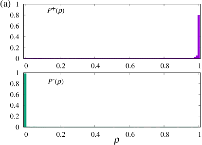
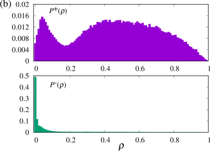
Figure 1: Examples of $P_{\rho}^{\pm}(\rho)$. (a) $\alpha=0.5$, $K=10$, $\theta=0.05$, $p_{\mathrm{TP}}=0.98$, and $p_{\mathrm{FP}}=0.01$, and (b) $\alpha=0.5$, $K=10$, $\theta=0.1$, $p_{\mathrm{TP}}=0.9$, and $p_{\mathrm{FP}}=0.05$.

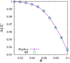
Figure 2: (a) Comparison of AUCs evaluated by the replica method and BP algorithm for $\alpha=0.5$, $K=10$, $p_{\mathrm{TP}}=0.95$, $p_{\mathrm{FP}}=0.1$. The results of the BP algorithm are averaged over 100 samples at $N=1000$, and the results of the replica method are averaged over 10 random number sequences in the population dynamics. (b) Prevalence dependence of the cutoff that maximizes the expected Youden index at $\alpha=0.5$, $K=10$, $p_{\mathrm{TP}}=0.95$, $p_{\mathrm{FP}}=0.1$. The slope of the dotted line is 1.

Fig. 1 shows the examples of $P_{\rho}^{\pm}(\rho)$ calculated by the population dynamics, where the parameters are set as $N_{\pi}=10^{4}$, $T=10^{7}$, and $R=10^{5}$. Distribution (a) is for $\alpha=0.5$, $\theta=0.05$, $p_{\mathrm{TP}}=0.98$, and $p_{\mathrm{FP}}=0.01$, which is an example for small prevalence and small error probabilities, and (b) is for $\alpha=0.5$, $\theta=0.1$, $p_{\mathrm{TP}}=0.9$, and $p_{\mathrm{FP}}=0.05$, which is an example for relatively large prevalence and large error probabilities. In the case of (a), the peaks of the two distributions are far apart, and the two populations can be separated with high accuracy. Meanwhile, in case (b), the posterior probability for the defective items is widely distributed.

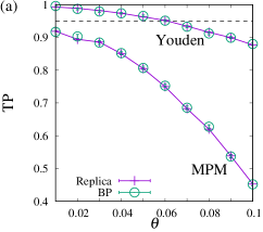
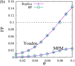
Figure 3: Comparison of (a) TP and (b) FP under the cutoff of $\theta$ (Youden) and 0.5 (MPM) for $\alpha=0.5$, $p_{\mathrm{TP}}=0.95$, and $p_{\mathrm{FP}}=0.1$. The dashed horizontal lines represent the characteristics of the original test; $p_{\mathrm{TP}}$ for (a) and $p_{\mathrm{FP}}$ for (b).

IV-B Comparison with the BP algorithm

We have imposed some assumptions in our analysis so far. Here, we confirm the adequacy of these assumptions by comparing the analytical results with those obtained using the BP algorithm [39, 19]. The details of the BP algorithm and its correspondence with the replica analysis are discussed in Sec.V. When the pools are randomly constructed under the constraints on $K\ll N$ and $C\ll N$, it is known that the exact posterior marginals can be obtained by the BP algorithm at sufficiently large values of $N$ and $M$ while setting the ratio $\alpha=M/N\sim O(1)$.

In Fig.2(a), the AUC derived using the replica method and the associated population dynamics are compared with that calculated using the BP algorithm at $\alpha=0.5$, $p_{\mathrm{TP}}=0.95$, and $p_{\mathrm{FP}}=0.1$. For BP, the number of items is set to $N=1000$, and the results are averaged over 1000 samples of the test results $\bm{y}$ and pooling method $\bm{c}$. For calculating the AUC using BP, we set the true state of the items to satisfy $\sum_{i=1}^{N}x_{i}^{(0)}=N\theta$ and fix a pooling method $\bm{c}$; then, we generate one instance of $\bm{y}$ according to the likelihood. TP and FP for each cutoff are calculated using the true state of the items and the posterior probability by BP. As shown in 2(a), the theoretical result, denoted by ’Replica,’ coincides with the algorithmic result of BP, denoted by ’BP,’ where the result of BP is averaged over 100 samples of $\bm{y}$, $\bm{c}$, and $\bm{x}^{(0)}$. In Fig. 2(b), the dependence on the prevalence of the cutoff, which maximizes the expected Youden index calculated by the replica method, is shown. For comparison, we show the diagonal dashed line with gradient 1. As discussed in Sec. III, the cutoff that maximizes the expected Youden index is coincident with the prevalence. This observation also supports the adequacy of our analysis.

In Fig.3, the cutoff-dependent properties, (a) true positive rate (TP) and (b) false positive rate (FP), are shown in comparison with the results of the replica method and BP algorithm, where the lines with labels ‘Youden’ and ‘MPM’ indicate the TP and FP under the cutoff of $\theta$ and $0.5$, respectively. The cutoff-dependent property evaluated by the replica method also matches with that calculated by the BP algorithm. The horizontal dashed lines represent the original test properties, (a) $p_{\mathrm{TP}}$, (b) $p_{\mathrm{FP}}$, and $\mathrm{TP}>p_{\mathrm{TP}}$ and $\mathrm{FP}<p_{\mathrm{FP}}$ indicate that a part of the test errors are corrected by the group testing. As discussed in Sec. III, the MPM estimator prefers to decrease FP, and as a tradeoff, the TP obtained using the MPM estimator is lower than that in the Youden index maximization. In the case of Youden index maximization, the false positive and false negative can be corrected simultaneously when $\theta<0.06$. This result also matches the behavior of the BP algorithm.

IV-C Effectiveness of the group testing measured by ROC curve

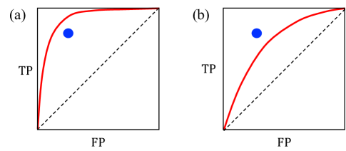
Figure 4: Our criterion for the effectiveness of group testing. As shown in (a), when the original test property (dot at $(p_{\mathrm{FP}},p_{\mathrm{TP}})$) is below the ROC curve (solid line), we consider the group testing to be superior to the original test. In contrast, when the original test property is above the ROC curve, as shown in (b), we consider the group testing to be inferior to the original test.

We discuss the parameter region in which the identification performance of the group testing under the Bayesian optimal setting is superior to that of the original test. We introduce the criterion shown in Fig.4 for the quantitative comparison between the original test and the group testing. The solid line in Fig. 4 is an example of the ROC curve obtained with Bayesian group testing, and the dot located at $(p_{\mathrm{FP}},p_{\mathrm{TP}})$ represents an example of the original test property. The better test method approaches the ROC curve toward the point $(\mathrm{FP}=0$,$\mathrm{TP}=1)$; hence, we consider the group test under the Bayesian optimal setting superior to the original test when the dot is below the ROC curve, as shown in Fig. 4 (a). In the contrasting situation, the dot is over the ROC curve, as shown in Fig. 4 (b), and we consider that the group test cannot exceed the original test performance. The ROC curve is obtained with the distributions of the posterior marginal probabilities derived by the replica method under the Bayesian optimal setting $P_{\rho}^{\pm}(\rho)$.

Fig.5 shows the phase diagrams based on the criterion at $\alpha=0.5$ and $K=10$ for (a) $\theta=0.05$ and (b) $\theta=0.07$, where the shaded area represents the region where the group testing under the Bayesian optimal setting is effective. Here, we do not consider the region $p_{\mathrm{TP}}<0.5$ and $p_{\mathrm{FP}}>0.5$, where the test performance is worse than the random decision on the items’ states. The effective region shrinks as the prevalence increases, and extends as the number of tests increases. As $p_{\mathrm{TP}}$ decreases, the group testing performance becomes inferior to that of the original test for a small region $p_{\mathrm{FP}}$. This is because a part of the true negatives is erroneously changed to positive while correcting the false negatives, and the fraction of false results is larger than $p_{\mathrm{FP}}$.

As discussed in Sec.III, the Bayesian optimal setting yields the largest value of the expected AUC when the correlation between the items’ states is ignored. Therefore, in the model mismatch case, the effective regions shown in Fig.5 are smaller than that in the Bayesian optimal setting. In the parameter region where the group testing under the Bayesian optimal setting is inferior to the original test, it is expected that the group testing under any other setting is also inferior to the original test. We can utilize the phase diagrams of the Bayes optimal setting as a guide to interpret which parameter region is appropriate for the group testing.

Figure 5: At $\alpha=0.5$ and $K=10$, the identification performance of the Bayesian group testing exceeds that of the original test in the shaded parameter region. (a) and (b) are for $\theta=0.05$ and $\theta=0.07$, respectively.

V Interpretation of the replica analysis from the correspondence with the BP algorithm

V-A BP algorithm

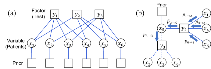
Figure 6: (a) Factor graph representation of the posterior distribution for pools on which the tests are performed. (b) Tree approximation of the graph and messages defined on the edges.

The meaning of the distributions $\pi$ and $\hat{\pi}$ in the replica method and the corresponding population dynamics can be interpreted by utilizing the correspondence between the replica method and BP algorithm. The derivation of the BP algorithm for the group testing can be referred from [9, 39, 18, 19], and is briefly explained here. Fig.6(a) illustrates a graphical representation of the posterior distribution (3) for the group testing, where the pools on which the tests are not performed ($\nu$-th pool with $c_{\nu}=0$) are not depicted. The variable nodes ($\bigcirc$) and factor nodes ($\square$) represent the items’ states and the test results performed on the pools, respectively. The edges represent the pooling method; the edge between the 1st factor node and 1st item indicates that the 1st item is contained in the 1st pool. The degrees of factor nodes and variable nodes correspond to the pool size $K$ and overlap $C$. In the derivation of the BP algorithm, we locally impose a tree approximation as shown in Fig.6(b), and define two messages $p_{i\to\nu}(x_{i})$ and $\tilde{p}_{\nu\to i}(x_{i})$ on the edge that connects $\nu$-th factor node and $i$-th variable node. Intuitively, these messages correspond to the marginal posterior distributions of $x_{i}$ before and after performing the $\nu$-th test under the tree approximation. The BP algorithm describes the constructive manner of the joint distribution on the tree as

$$\tilde{p}_{\nu\to i}(x_{i}) \propto\sum_{\bm{x}\backslash x_{i}}\tilde{f}(y_{\nu}|\bm{x}_{(\nu)})\prod_{j\in{\cal L}(\nu)\backslash i}p_{j\to\nu}(x_{j})$$ (55)

$$p_{i\to\nu}(x_{i}) \propto\phi(x_{i})\prod_{\eta\in{\cal G}(i)\backslash\nu}\tilde{p}_{\eta\to i}(x_{i}),$$ (56)

where we denote $\tilde{f}(y_{\nu}|\bm{x}_{(\nu)})\equiv f(y_{\nu}|c_{\nu}=1,\bm{x}_{(\nu)})$ for conciseness. As mentioned earlier, ${\cal L}(\nu)$ and ${\cal G}(i)$ are the set of item labels in the $\nu$-th pool and the set of pool labels $i$-th item is contained, respectively. Using these messages, the marginalized posterior distribution is given by

$$p_{i}(x_{i})\propto\phi(x_{i})\prod_{\eta\in{\cal G}(i)}\tilde{p}_{\eta\to i}(x_{i}).$$ (57)

On the tree graphs, (57) describes the exact marginal distribution, and to obtain (57), we need to propagate the messages on the tree once starting from the arbitrary root. For the general graphs, we need to recursively update the messages for sufficient time steps until convergence; hence, hereafter, we denote the messages at time step $t$ as $\tilde{p}_{\nu\to i}^{(t)}$ and $p_{i\to\nu}^{(t)}$. In the case of the group testing with random pools, the BP algorithm is expected to provide exact values of the posterior marginals at $N,~{}M\to\infty$ keeping $\alpha=M/N$ finite.

The messages are defined for the binary variables as defective or non-defective; hence, they are represented by the $[0,1]-$Bernoulli parameters $\{m_{j\to\nu}^{(t)}\}$ and $\{\tilde{m}_{\nu\to i}^{(t)}\}$, which are called the F-cavity fields and V-cavity fields, respectively, as

$$p_{j\to\nu}^{(t)}(x_{i}) =(1-m_{j\to\nu}^{(t)})(1-x_{i})+m_{j\to\nu}^{(t)}x_{i}$$ (58)

$$\tilde{p}_{\nu\to i}^{(t)}(x_{i}) =(1-\tilde{m}_{\nu\to i}^{(t)})(1-x_{i})+\tilde{m}_{\nu\to i}^{(t)}x_{i}.$$ (59)

The time evolution of these Bernoulli parameters are derived from (55)–(56) as

$$m_{j\to\nu}^{(t)}=\frac{\theta\displaystyle\prod_{\eta\in{\cal G}(i)\backslash\nu}\tilde{m}^{(t-1)}_{\eta\to i}}{(1-\theta)\displaystyle\prod_{\eta\in{\cal G}(i)\backslash\nu}(1-\tilde{m}_{\eta\to i}^{(t-1)})+\theta\prod_{\eta\in{\cal G}(i)\backslash\nu}\tilde{m}_{\eta\to i}^{(t-1)}}$$ (60)

$$\tilde{m}_{\nu\to i}^{(t)}$$ (61)

$$=\!\frac{U_{\nu}}{U_{\nu}\left\{2\!-\!\!\!\displaystyle\prod_{j\in{\cal L}(\nu)\!\backslash i}(1\!-\!m_{j\to\nu}^{(t-1)})\right\}\!+\!W_{\nu}\!\!\!\displaystyle\prod_{j\in{\cal L}(\nu)\!\backslash i}(1\!-\!m_{j\to\nu}^{(t-\!1)})},$$

where

$$U_{\nu} =p_{\mathrm{TP}}y_{\nu}+(1-p_{\mathrm{TP}})(1-y_{\nu}),$$ (62)

$$W_{\nu} =p_{\mathrm{FP}}y_{\nu}+(1-p_{\mathrm{FP}})(1-y_{\nu}).$$ (63)

We denote the obtained cavity fields after sufficient updates as $\{m_{j\to\nu}\}$ and $\{\tilde{m}_{\nu\to i}\}$. The marginal posterior distribution (57) is expressed using the Bernoulli parameter $m_{i}$, which is given by the F-cavity fields as

$$m_{i}=\frac{\theta\prod_{\eta\in{\cal G}(i)}\tilde{m}_{\eta\to i}}{(1-\theta)\prod_{\eta\in{\cal G}(i)}(1-\tilde{m}_{\eta\to i})+\theta\prod_{\eta\in{\cal G}(i)}\tilde{m}_{\eta\to i}}.$$ (64)

(64) is the estimate of the marginal posterior probability $\rho_{i}$; hence, using (64) and the appropriate cutoff, one can obtain the items’ states under the given test results $\bm{y}$ and pooling method $\bm{c}$. Furthermore, the Bayes factor (23) can be calculated using the BP algorithm as

$$\mathrm{BF}_{i}^{10}=\prod_{\eta\in{\cal G}(i)}\frac{\tilde{m}_{\eta\to i}}{1-\tilde{m}_{\eta\to i}}.$$ (65)

The decision based on the Bayes factor (27) can be easily implemented by the BP algorithm using the expression (65).

An advantage of the BP algorithm is that the updating of the messages is implemented using the matrix products. In Algorithm 2, the BP algorithm using the matrix representation is summarized, where the messages are represented in the matrix forms $\bm{M}\in\mathbb{R}^{N\times M}$ and $\tilde{\bm{M}}\in\mathbb{R}^{M\times N}$, where $M_{i\nu}=m_{i\to\nu}$ and $\tilde{M}_{\nu i}=\tilde{m}_{\nu\to i}$. In Algorithm 2, we introduce the matrix $\bm{F}\in\{0,1\}^{M\times N}$ representing the pooling method $\bm{c}$, where $F_{\nu i}=1$ when $\nu\in{\cal G}(i)$ or $i\in{\cal L}(\nu)$, and $F_{\nu i}=0$ otherwise. For convenience, we define an operator $\Pi(\bm{A})$ for an arbitrary $M\times N$ matrix $\bm{A}$ that outputs an $N$-dimensional vector whose $i$-th component is $\prod_{\mu=1}^{M}A_{\mu i}$, and $\bm{1}_{M\times N}$ is an $M\times N$ matrix whose components are 1. The notations $\circ$ and $\oslash$ represent the Hadamard product and Hadamard division, respectively, namely $(A\circ B)_{ij}=A_{ij}B_{ij}$ and $(A\oslash B)_{ij}=A_{ij}/B_{ij}$, where $A$ and $B$ are matrices of the same size.

Algorithm 2 BP algorithm for group testing (matrix representation)

1:$p_{\mathrm{TP}}$, $p_{\mathrm{FP}}$, $\theta$, $\bm{y}$, $\bm{F}$, $\varepsilon$

2:$\bm{m}$

3:Initialize:

4:      $\bm{Y}\leftarrow\bm{y}\bm{1}_{1\times N}$ $\bm{U}\leftarrow p_{\mathrm{TP}}\bm{Y}+(1-p_{\mathrm{TP}})(\bm{1}_{M\times N}-\bm{Y})$ $\bm{W}\leftarrow p_{\mathrm{FP}}\bm{Y}+(1-p_{\mathrm{FP}})(\bm{1}_{M\times N}-\bm{Y})$ $t\leftarrow 0$$\triangleright$ Iteration counting
$s\leftarrow 0$$\triangleright$ Indicator of the convergence
$\bm{M}^{(0)}\leftarrow$ Initial values from $[0,1]^{N\times M}$
$\bm{M}^{(0)}\leftarrow\bm{M}^{\!(0)}\circ\bm{F}^{\mathrm{T}}$$\triangleright$ Remove undefined messages
$\widetilde{\bm{M}}^{(0)}\leftarrow$ Initial values from $[0,1]^{M\times N}$
$\widetilde{\bm{M}}^{(0)}\leftarrow\widetilde{\bm{M}}^{(0)}\circ\bm{F}$$\triangleright$ Remove undefined messages

5:while $s=0$ do$\triangleright$ BP loop start

6:     $t\leftarrow t+1$

7:     $\bm{Q}^{(t)}\!\leftarrow\!\!(\Pi(\bm{1}_{\!N\!\times\!M}\!-\!\bm{M}^{(t-1)})\bm{1}_{\!1\!\times\!N})\oslash\!(\bm{1}_{\!N\!\times\!M}\!-\!\bm{M}^{(t-1)})^{\mathrm{T}}$

8:     $\widetilde{\bm{M}}^{(t)}\!\!\leftarrow\!\!\bm{F}\circ(\bm{U}\oslash(\bm{U}+(\bm{U}\circ(\bm{1}_{M\times N}-\bm{Q}^{(t)})+\bm{W}\circ\bm{Q}^{(t)}))$

9:     $\widetilde{\bm{Q}}^{(t)}_{+}\!\!\leftarrow\!\!(\Pi(\widetilde{\bm{M}}^{(t-1)}\!+\!(\bm{1}_{\!M\!\times\!N}\!-\!\bm{F}))\bm{1}_{\!1\!\times\!M})\oslash\!(\widetilde{\bm{M}}^{(t-1)}\!+\!(\bm{1}_{\!M\!\times\!N}\!-\!\bm{F}))^{\mathrm{T}}$

10:     $\widetilde{\bm{Q}}^{(t)}_{-}\!\!\leftarrow\!\!(\Pi(\bm{1}_{\!M\!\times\!N}\!-\!\widetilde{\bm{M}}^{(t-1)})\bm{1}_{\!1\!\times\!M})\oslash(\bm{1}_{\!M\!\times\!N}\!-\!\widetilde{\bm{M}}^{(t-1)})^{\mathrm{T}}$

11:     $\bm{M}^{(t)}\leftarrow\bm{F}^{\mathrm{T}}\circ(\theta\bm{Q}^{(t)}_{+}\oslash(\theta\bm{Q}^{(t)}_{+}+(1-\theta)\bm{Q}^{(t)}_{-}))$

12:     $dM^{(t)}\leftarrow||\bm{M}^{(t)}\!-\!\bm{M}^{(t-1)}||_{2}$

13:     $d\widetilde{M}^{(t)}\leftarrow||\widetilde{\bm{M}}^{(t)}\!-\!\widetilde{\bm{M}}^{(t-1)}||_{2}$

14:     $s\leftarrow\mathbb{I}(dM^{(t)}<NM\varepsilon$ and $d\widetilde{M}^{(t)}<NM\varepsilon)$

15:end while

16:$\bm{m}\leftarrow\theta\Pi(\widetilde{\bm{M}}^{(t)}+(\bm{1}_{M\times N}-\bm{F}))\oslash(\theta\Pi(\widetilde{\bm{M}}^{(t)}+(\bm{1}_{M\times N}-\bm{F}))+(1-\theta)\Pi(\bm{1}_{M\times N}-\widetilde{\bm{M}}^{(t)}))$

V-B Expectation of BP trajectory and replica analysis

The cavity fields in the BP algorithm are random variables that depend on the realization of the randomness $\bm{y}$ and $\bm{c}$, where $\bm{y}$ is generated by the true items’ states $\bm{x}^{(0)}$. Let us define the probability distribution of the F-cavity fields for defective and non-defective items at step $t$ as

$$\pi_{\mathrm{BP}}^{(t)}(m|1)=E_{\bm{y},\bm{c},\bm{x}^{(0)}|x_{i}^{(0)}=1}[\delta(m^{(t)}_{i\to\nu}-m)]$$ (66)

$$\pi_{\mathrm{BP}}^{(t)}(m|0)=E_{\bm{y},\bm{c},\bm{x}^{(0)}|x_{i}^{(0)}=0}[\delta(m^{(t)}_{i\to\nu}-m)],$$ (67)

and that of the V-cavity fields as

$$\tilde{\pi}_{\mathrm{BP}}^{(t)}(\tilde{m}|1)=E_{\bm{y},\bm{c},\bm{x}^{(0)}|x_{i}^{(0)}=1}[\delta(\tilde{m}^{(t)}_{\nu\to i}-m)]$$ (68)

$$\tilde{\pi}_{\mathrm{BP}}^{(t)}(\tilde{m}|0)=E_{\bm{y},\bm{c},\bm{x}^{(0)}|x_{i}^{(0)}=0}[\delta(\tilde{m}^{(t)}_{\nu\to i}-m)],$$ (69)

where $E_{\bm{y},\bm{c},\bm{x}^{(0)}|x_{i}^{(0)}=1}[\cdot]$ and $E_{\bm{y},\bm{c},\bm{x}^{(0)}|x_{i}^{(0)}=0}[\cdot]$ denote the expectation with respect to randomness under the constraint that $x_{i}^{(0)}=1$ and $x_{i}^{(0)}=0$, respectively. Here, we assume that (66)–(69) do not depend on $i$, and the dependency between the messages can be ignored. Under this assumption, we can show that the time evolution equations of the distributions (66)–(69) correspond to the recursive updating of the distributions derived by the replica method as follows. Assuming the independence of $\tilde{m}_{\eta\to i}$ for $\eta\in{\cal G}(i)$, (68) is transformed as

$$\pi_{\mathrm{BP}}^{(t)}(m|1)$$

$$=\!E_{\bm{y},\bm{c},\bm{x}^{(0)}\!|x_{i}^{(0)}\!=1}\!\!\left[\delta\!\left(\!m\!-\!\frac{\rho\displaystyle\prod_{\eta\in{\cal G}(i)\backslash\nu}\tilde{m}_{\eta\to i}}{(1\!-\!\rho)\!\!\!\!\!\!\!\displaystyle\prod_{\eta\in{\cal G}(i)\backslash\nu}\!\!\!\!\!\!(1\!-\!\tilde{m}_{\eta\to i})\!+\!\rho\!\!\!\!\!\!\!\prod_{\eta\in{\cal G}(i)\backslash\nu}\!\!\!\!\!\!\tilde{m}_{\eta\to i}}\!\right)\!\right]$$

$$=\int\prod_{\gamma=1}^{C-1}d\tilde{m}_{\gamma}\tilde{\pi}_{\mathrm{BP}}^{(t-1)}(\tilde{m}_{\gamma}|1)\delta\left(m-\mu(\tilde{\bm{m}}_{(C-1)})\right),$$ (70)

where $\tilde{\bm{m}}_{(C-1)}=[\tilde{m}_{1},\cdots,\tilde{m}_{C-1}]^{\mathrm{T}}$ and $\mu(\tilde{\bm{m}}_{(C-1)},\theta)$ is given by (47). Equation (70) corresponds to the recursive relationship of the distribution derived using the replica method (54) at $x=1$. The same relationship holds for $\pi_{\mathrm{BP}}^{(t)}(m|0)$ based on the above discussion.

For the derivation of the V-cavity field distribution, we need to consider the generative process of $\bm{y}$. When $x_{i}=1$, the test result on the $\nu$-th pool $y_{\nu}$, which contains the $i$-th item, is 1 with probability $p_{\mathrm{TP}}$ and 0 with probability $1-p_{\mathrm{TP}}$, irrespective of the states of the other items in the pool. Therefore, under the assumption of independency of the V-cavity fields, (68) is given by

$$\tilde{\pi}^{(t)}_{\mathrm{BP}}(\tilde{m}|1)=\int\prod_{\kappa=1}^{K-1}dm_{\kappa}\sum_{x_{1},\cdots,x_{K-1}}\prod_{\kappa=1}^{K-1}\phi(x_{\kappa})\pi^{(t-1)}_{\mathrm{BP}}(m_{\kappa}|x_{\kappa})$$

$$\hskip 14.22636pt\times\Big{\{}p_{\mathrm{TP}}\delta\left(\tilde{m}-\tilde{\mu}(p_{\mathrm{TP}},p_{\mathrm{FP}},\bm{m}_{(K-1)})\right)$$

$$\hskip 19.91684pt+(1\!-\!p_{\mathrm{TP}})\delta(\tilde{m}-\tilde{\mu}(1\!-\!p_{\mathrm{TP}},1\!-\!p_{\mathrm{FP}},\bm{m}_{(K\!-\!1)})\Big{\}},$$ (71)

where $\bm{m}_{(K-1)}=[m_{1},\cdots,m_{K-1}]^{\mathrm{T}}$, and $\tilde{\mu}(p_{\mathrm{TP}},p_{\mathrm{FP}},\bm{m}_{(K-1)})$ is given by (50). Equation (71) is equivalent to the analytical expression derived using the replica method (52). Meanwhile, when $x_{i}^{(0)}=0$, the test result $y_{\nu}$ is governed by the other items in the pool. When all items are non-defective, $y_{\nu}=1$ and $y_{\nu}=0$ are realized with probability $p_{\mathrm{FP}}$ and $1-p_{\mathrm{FP}}$, respectively. If there is at least one defective item in the $\nu$-th pool, $y_{\nu}=1$ and $y_{\nu}=0$ are realized with probability $p_{\mathrm{TP}}$ and $1-p_{\mathrm{TP}}$, respectively. Thus, only the all-zero case differs from the distribution $\tilde{\pi}_{\mathrm{BP}}^{(t)}(\tilde{m}|1)$. In summary, we obtain

$$\tilde{\pi}_{\mathrm{BP}}^{(t)}(\tilde{m}|0)=\tilde{\pi}^{(t)}_{\mathrm{BP}}(\tilde{m}|1)+\int\prod_{\kappa=1}^{K-1}dm_{\kappa}\pi_{\mathrm{BP}}^{(t)}(m_{\kappa}|0)(1-\theta)^{K-1}$$

$$\times\Big{\{}(p_{\mathrm{FP}}\!-\!p_{\mathrm{TP}})\delta\left(\tilde{m}-\tilde{\mu}(p_{\mathrm{TP}},p_{\mathrm{FP}},\bm{m}_{(K-1)})\right)$$

$$\hskip 5.69046pt+(p_{\mathrm{TP}}\!-\!p_{\mathrm{FP}})\delta\left(\tilde{m}-\tilde{\mu}(1\!-\!p_{\mathrm{TP}},1\!-\!p_{\mathrm{FP}},\bm{m}_{(K\!-\!1)})\right)\}$$ (72)

Equation (72) is equivalent to (53) in the replica method.

In fact, the BP algorithm is defined for one realization of the randomness $\bm{y}$, $\bm{c}$, and $\bm{x}^{(0)}$. However, because of the law of large numbers, it is expected that the empirical distributions of the cavity fields for a single typical samples of $\bm{y},\bm{c},\bm{x}^{(0)}$ converge in probability as

$$\frac{1}{N\theta C}\sum_{i=1}^{N}\!\sum_{\nu\in{\cal G}(i)}\!\!x_{i}^{(0)}\delta(m^{(t)}_{i\to\nu}\!-\!m) \xrightarrow{N\to\infty}\pi_{\mathrm{BP}}^{(t)}(m|1)$$ (73)

$$\frac{1}{N\theta C}\sum_{i=1}^{N}\!\sum_{\nu\in{\cal G}(i)}\!\!(1\!-\!x_{i}^{(0)})\delta(m^{(t)}_{i\to\nu}\!-\!m) \xrightarrow{N\to\infty}\pi_{\mathrm{BP}}^{(t)}(m|0)$$ (74)

$$\frac{1}{MK\theta}\!\sum_{\nu=1}^{M}\!\sum_{i\in{\cal M}(\nu)}\!\!\!x_{i}^{(0)}\delta(\tilde{m}^{(t)}_{\nu\to i}\!-\!\tilde{m}) \xrightarrow{N\to\infty}\tilde{\pi}_{\mathrm{BP}}^{(t)}(\tilde{m}|1)$$ (75)

$$\frac{1}{MK\theta}\!\sum_{\nu=1}^{M}\!\sum_{i\in{\cal M}(\nu)}\!\!\!(1\!-\!x_{i}^{(0)})\delta(\tilde{m}^{(t)}_{i\to\nu}\!-\!\tilde{m}) \xrightarrow{N\to\infty}\tilde{\pi}_{\mathrm{BP}}^{(t)}(\tilde{m}|0).$$ (76)

for any $t$. Eqs. (73)-(76) are known as self-averaging property. In Figs.7 and 8, the time evolution of the logarithmic values of $\pi^{(t)}(\mu|x)$ and $\hat{\pi}^{(t)}(\hat{\mu}|x)$ ($x\in\{0,1\}$) in the replica method and that of $\pi_{\mathrm{BP}}^{(t)}(\mu|x)$ and $\hat{\pi}^{(t)}_{\mathrm{BP}}(\hat{\mu}|x)$ in the BP algorithm are compared at $\alpha=0.5$, $K=10$, $p_{\mathrm{TP}}=0.9$, and $p_{\mathrm{FP}}=0.05$. The distribution in BP is calculated as the L.H.S. of (73)–(76) at $N=5\times 10^{5}$ for a single sample of $\bm{y},\bm{c},\bm{x}^{(0)}$. As the initial condition, we set all members of the populations $\bm{\pi}^{+}$ and $\bm{\pi}^{-}$ at $\theta$ and that of populations $\hat{\bm{\pi}}^{+}$ and $\hat{\bm{\pi}}^{-}$ at 0.5 in Algorithm 1. Correspondingly, we set $m_{i\to\nu}=\theta$ and $\hat{m}_{\nu\to i}=0.5$ as the initial condition in BP for all pairs of $(i,\nu)$, where $i\in{\cal L}(\nu)$ or $\nu\in{\cal G}(i)$. The difference between the distribution by PD and that by BP is $O(10^{-2})$ at the maximum; hence, it is considered that the assumption of the self-averaging property is adequate. In particular, the bifurcation in the distribution that appears at $t\leq 5$ for $\pi(\mu|x)$ and $\pi_{\mathrm{BP}}(m|x)$, and that appears at $t\leq 4$ for $\hat{\pi}(\hat{\mu}|x)$ and $\hat{\pi}_{\mathrm{BP}}(\hat{m}|x)$ entirely match each other.

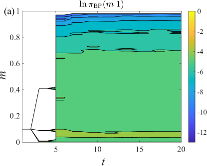
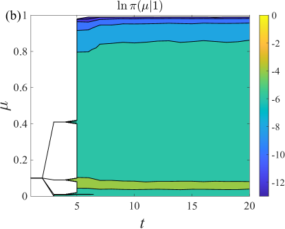
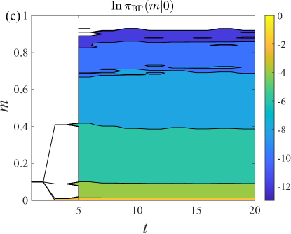
Figure 7: Time evolution of the logarithmic distributions $\pi_{\mathrm{BP}}(m|x)$ and $\pi(\mu|x)$ for $x\in\{0,1\}$ at $\alpha=0.5$, $K=10$, $p_{\mathrm{TP}}=0.9$, and $p_{\mathrm{FP}}=0.05$. In BP, the distributions are calculated under a fixed randomness at $N=5\times 10^{5}$.

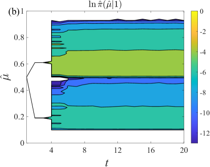
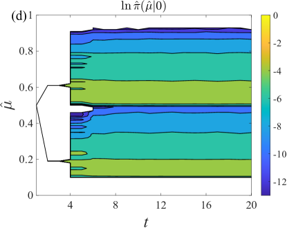
Figure 8: Time evolution of the logarithmic distributions $\hat{\pi}_{\mathrm{BP}}(\hat{m}|x)$ and $\hat{\pi}(\hat{\mu}|x)$ for $x\in\{0,1\}$ at $\alpha=0.5$, $K=10$, $p_{\mathrm{TP}}=0.9$, and $p_{\mathrm{FP}}=0.05$. In BP, the distributions are calculated under a fixed randomness at $N=5\times 10^{5}$.

VI Summary and Conclusion

In this study, we analyzed a group testing model under the Bayesian optimal setting. We demonstrated that the posterior AUC takes the maximum value when the marginal posterior probability under the Bayesian optimal setting is used as the diagnostic variable. Furthermore, we derived an optimal cutoff based on the expected risk; in particular, the estimator defined by the cutoff that equals the prevalence maximizes an unbiased estimator of the expected Youden index. The derived cutoff can be interpreted by using the Bayes factor. To understand the performance of the group testing under the Bayesian optimal setting, we applied the replica method in statistical physics to the group testing model. The obtained result matched the result of the algorithm, which supports our analysis. Based on the consideration of the Bayesian optimal setting, the obtained results are expected to provide an estimation of the upper bound for the group testing performance.

In the following, we summarize the assumptions introduced in our problem setting, and explain how we can approach these assumptions to achieve realistic settings in the future.

$\bullet$ A1  

The pools containing at least one defective item are regarded as positive.

When we consider the clinical testing where the specimens of the patients are pooled, the dilution effect is negligible. To consider this effect, a group testing model that has a detection limit is proposed [40]. Furthermore, in applying the group testing to the genome sequence processing, semi-quantitative group testing is a realistic setting rather than the logical sum rule [41].

$\bullet$ A2  

Independence of the tests

When the specimens collected from the defected patients do not contain sufficient amounts of the pathogen to exceed the detection threshold, the results of the test performed on the pools that contain insufficient specimen quantity can be non-defective with a high probability when compared with other pools. This is an example that violates the assumption of the independence and identicality of the tests.

In the case of the diagnostic test for intrathoracic tuberculosis in children, a multiple sampling and pooling method for specimens collected using different methods such as gastric aspirate, a nasopharyngeal aspirate, and induced sputum has been discussed to obtain greater specimen volume [42]. The combinatorial formulation of the collection method of the specimen and the subsequent group testing are expected to provide more realistic models.

$\bullet$ A3-4

Prior knowledge of the true positive probability, false positive probability, and prevalence

The test properties $p_{\mathrm{TP}}$ and $p_{\mathrm{FP}}$ and the prevalence $\theta$ are generally unknown; hence, an estimation procedure is required. There are various methods to estimate the true positive probability and false positive probability in a diagnostic test, and the utilization of these methods before performing the group testing is straightforward. For instance, in previous studies, the estimation of parameters was studied by introducing Bayesian inference [43]. To simultaneously estimate these parameters and the items’ states in the group testing, the expectation-maximization method and hierarchical Bayes approach [19] can be combined with the BP algorithm.

$\bullet$ A5  

Equal pretest probability of all items

In the BP algorithm mentioned in Sec.IV-A, the evaluation of the marginal posterior probability under the item-dependent prior distribution is possible. Furthermore, as a realistic setting, the regional-dependence of the prevalence is considered by introducing the mixed effect model [44]. However, the cutoff determination and performance evaluation in the case of inhomogeneous prevalence should be discussed.

Details of the replica method

We introduce the following expression of the Kronecker’s delta:

$$\delta(a,b)=\oint_{|z|=1}\frac{dz}{2\pi\sqrt{-1}z^{b+1}}z^{a}.$$ (77)

Applying (77) to the joint distribution for the randomness (32), we obtain:

$$P_{\mathrm{rand}}(\bm{y},\bm{c},\bm{x}^{(0)})$$

$$=\frac{1}{\cal D}\prod_{j=1}^{N}\oint\frac{dz_{j}}{2\pi\sqrt{-1}z_{j}^{C+1}}z_{j}^{\sum_{\mu\in{\cal G}(j)}c_{\mu}}f(\bm{y}|\bm{c},\bm{x}^{(0)})\phi(\bm{x}^{(0)}),$$ (78)

where the integral representation of Kronecker’s delta is introduced. The procedure for calculating (42) is summarized in three steps.

$\bullet$ 1

Summation of $\bm{y}$ and $\bm{c}$

$\bullet$ 2

Integration of $\bm{z}$, which appears in the integral representation of Kronecker’s delta in (78)

$\bullet$ 3

Approximation using the saddle point method under RS assumption

We explain these procedures below.

-A Summation of $\bm{y}$ and $\bm{c}$

Summation over $\bm{y}$ and $\bm{c}$ leads to the following expression:

$${\cal M}_{ik}^{+}(n) =\frac{1}{{\cal D}}\oint\frac{\prod_{j=1}^{N}dz_{j}z_{j}^{-(C+1)}}{(2\pi\sqrt{-1})^{N}}\sum_{\{\bm{x}^{(a)}\}}x_{i}^{(0)}x_{i}^{(1)}\cdots x_{i}^{(k)}$$

$$\times\phi(\{\bm{x}^{(a)}\})\prod_{\nu=1}^{N_{p}}\left[1+\prod_{j\in{\cal L}(\nu)}^{K}z_{j}W_{n}(\tilde{\bm{x}}_{(\mu)})\right].$$ (79)

Here, $\tilde{\bm{x}}_{i}=\{x_{i}^{(0)},x_{i}^{(1)},\cdots,x_{i}^{(n)}\}\in\{0,1\}^{n+1}$ is the replica vector of the $j$-th variable, and $\tilde{\bm{x}}_{(\nu)}=\{\tilde{\bm{x}}_{1(\nu)},\cdots,\tilde{\bm{x}}_{K(\nu)}\}$. We set $\phi(\{\bm{x}^{(a)}\})=\prod_{a=0}^{n}\phi(\bm{x}^{(a)})$, and $W_{n}(\tilde{\bm{x}}_{(\mu)})$ is defined as

$$W_{n}(\tilde{\bm{x}}_{(\mu)})=\prod_{a=0}^{n}\left\{p_{\mathrm{TP}}T(\bm{x}^{(a)}_{(\mu)})+p_{\mathrm{FP}}(1-T(\bm{x}^{(a)}_{(\mu)}))\right\}$$ (80)

$$+\prod_{a=0}^{n}\left\{(1-p_{\mathrm{TP}})T(\bm{x}^{(a)}_{(\mu)})+(1-p_{\mathrm{FP}})(1-T(\bm{x}^{(a)}_{(\mu)}))\right\}.$$

Furthermore, we introduce the dummy variables $\tilde{\bm{u}}_{j}=\{u_{j}^{(0)},u_{j}^{(1)},\cdots,u_{j}^{(n)}\}\in\{0,1\}^{n+1}$ for $j=1,\cdots,K$, and substitute the identity $\sum_{\tilde{\bm{u}}_{j}}\delta(\tilde{\bm{x}}_{j},\bm{u}_{j})=1$ for every $j\in\{1,\cdots,K\}$ as

$${\cal M}_{ik}^{+}(n) =\frac{1}{{\cal D}}\oint\frac{\prod_{j=1}^{N}dz_{j}z_{j}^{-(C+1)}}{(2\pi\sqrt{-1})^{N}}\!\!\!\sum_{\{\bm{x}^{(a)}\}}\!\!\!\phi(\{\bm{x}^{(a)}\})\prod_{\kappa=0}^{k}x_{i}^{(\kappa)}$$

$$\times\exp\left[\!\sum_{\nu=1}^{N_{p}}\!\prod_{j\in{\cal L}(\nu)}\!\left\{\!z_{j}\!\sum_{\tilde{\bm{u}}_{j}}\delta(\tilde{\bm{x}}_{j(\nu)},\tilde{\bm{u}}_{j})\!\right\}\!W_{n}(\{\tilde{\bm{u}}_{j}\})\!\right]$$

$$\simeq\frac{\prod_{i=1}^{N}dz_{i}z_{i}^{-(C+1)}}{(2\pi\sqrt{-1})^{N}}\sum_{\{\bm{x}^{(a)}\}}\phi(\{\bm{x}^{(a)}\})\prod_{\kappa=0}^{k}x_{i}^{(\kappa)}$$

$$\times\exp\left[\frac{N^{K}}{K!}\sum_{\{\tilde{\bm{u}}_{i}\}}\prod_{j=1}^{K}{\cal Q}_{n}(\tilde{\bm{u}}_{j})W_{n}(\{\tilde{\bm{u}}_{i}\})\right].$$ (81)

In deriving (81), we use the relationship $\sum_{\nu=1}^{N_{p}}1\sim\frac{1}{K!}\sum_{i_{1}=1}^{N}\cdots\sum_{i_{K}=1}^{N}1$, which is valid at sufficiently large values of $N$. Here, we set $\{\tilde{\bm{u}}_{i}\}=\{\tilde{\bm{u}}_{1},\cdots,\tilde{\bm{u}}_{K}\}$, and define the function ${\cal Q}_{n}(\tilde{\bm{u}})$ as follows:

$${\cal Q}_{n}(\tilde{\bm{u}})=\frac{1}{N}\sum_{i=1}^{N}z_{i}\prod_{a=0}^{n}\delta\left(x_{i}^{(a)},u^{(a)}\right).$$ (82)

(82) is a function of $\bm{z}$, $\{\bm{x}_{i}^{(a)}\}$, and $\tilde{\bm{u}}$, but it is expected that $\frac{1}{N}\sum_{i=1}^{N}z_{i}\prod_{a=0}^{n}\delta(x_{i}^{(a)},u^{(a)})\to E_{\bm{z},\tilde{\bm{x}}}[z\prod_{a=0}^{n}\delta(x^{(a)},u^{(a)})]$ holds for sufficiently large values of $N$; hence, we consider ${\cal Q}_{n}$ as a function of $\tilde{\bm{u}}$.

-B Integration of $\bm{z}$

We introduce the identity for all possible $\tilde{\bm{u}}\in\{0,1\}^{n+1}$:

$$1 =\int d{\cal Q}_{n}(\tilde{\bm{u}})\delta\left(\frac{1}{N}\sum_{i=1}^{N}z_{i}\prod_{a=0}^{n}\delta(x_{i}^{(a)},u^{(a)})-{\cal Q}_{n}(\bm{u})\right)$$

$$=\int\frac{d\hat{\cal Q}_{n}(\tilde{\bm{u}})d{\cal Q}_{n}(\tilde{\bm{u}})}{2\pi}$$

$$\times\!\exp\!\left\{\hat{\cal Q}_{n}(\tilde{\bm{u}})\!\left(\sum_{i=1}^{N}\!z_{i}\!\prod_{a=0}^{n}\!\delta(x_{i}^{(a)}\!\!,u^{(a)})\!-\!N{\cal Q}_{n}(\tilde{\bm{u}})\!\right)\!\right\},$$ (83)

where $\hat{\cal Q}_{n}(\tilde{\bm{u}})$ is the conjugate of ${\cal Q}_{n}(\tilde{\bm{u}})$. Substituting this into (81) and integrating $\bm{z}$, we obtain

$${\cal M}^{+}_{ik}(n) =\frac{1}{\cal D}\int d\bm{{\cal Q}}_{n}d\hat{\bm{{\cal Q}}}_{n}\exp\left(N\psi(\bm{{\cal Q}}_{n},\hat{\bm{{\cal Q}}}_{n})\right)$$ (84)

$$\times\frac{\sum_{\tilde{\bm{x}}_{i}}x_{i}^{(0)}x_{i}^{(1)}\cdots x_{i}^{(k)}\phi(\tilde{\bm{x}}_{i})\left(\hat{\cal Q}_{n}(\tilde{\bm{x}}_{i})\right)^{C}}{\sum_{\tilde{\bm{x}}_{i}}\phi(\tilde{\bm{x}}_{i})\left(\hat{\cal Q}_{n}(\tilde{\bm{x}}_{i})\right)^{C}},$$

where $\bm{{\cal Q}}_{n}=\{{\cal Q}_{n}(\tilde{\bm{u}})|\tilde{\bm{u}}\in\{0,1\}^{n+1}\}$, and $\hat{\bm{{\cal Q}}}_{n}=\{\hat{{\cal Q}}_{n}(\tilde{\bm{u}})|\tilde{\bm{u}}\in\{0,1\}^{n+1}\}$. The function $\psi(\bm{{\cal Q}}_{n},\hat{\bm{{\cal Q}}}_{n})$ is given by

$$\psi(\bm{{\cal Q}}_{n},\hat{\bm{{\cal Q}}}_{n}) ={\cal S}_{n}(\hat{\bm{{\cal Q}}}_{n})-{\cal V}(\bm{{\cal Q}}_{n},\hat{\bm{{\cal Q}}}_{n})+{\cal E}_{n}(\bm{{\cal Q}}_{n}),$$ (85)

where

$${\cal V}(\bm{{\cal Q}}_{n},\hat{\bm{{\cal Q}}}_{n}) =\sum_{\tilde{\bm{u}}}\hat{{\cal Q}}_{n}(\tilde{\bm{u}}){\cal Q}_{n}(\tilde{\bm{u}})$$ (86)

$${\cal S}_{n}(\hat{\bm{{\cal Q}}}_{n}) =\ln\sum_{\tilde{\bm{x}}}\prod_{a=0}^{n}\phi(\bm{x}^{(a)})(\hat{{\cal Q}}_{n}(\tilde{\bm{x}}))^{C}$$ (87)

$${\cal E}_{n}(\bm{{\cal Q}}_{n}) =\frac{N^{K-1}}{K!}\sum_{\tilde{\bm{u}}_{1},\cdots,\tilde{\bm{u}}_{K}}\prod_{k=1}^{K}{\cal Q}_{n}(\tilde{\bm{u}}_{k})W_{n}(\{\tilde{\bm{u}}_{k}\}).$$ (88)

Following the same procedure, ${\cal M}_{ik}^{-}$ is given by

$${\cal M}^{-}_{ik}(n) =\frac{1}{\cal D}\int d\bm{{\cal Q}}_{n}d\hat{\bm{{\cal Q}}}_{n}\exp\left(N\psi(\bm{{\cal Q}}_{n},\hat{\bm{{\cal Q}}}_{n})\right)$$ (89)

$$\times\frac{\sum_{\tilde{\bm{x}}_{i}}(1-x_{i}^{(0)})x_{i}^{(1)}\cdots x_{i}^{(k)}\phi(\tilde{\bm{x}}_{i})\left(\hat{\cal Q}_{n}(\tilde{\bm{x}}_{i})\right)^{C}}{\sum_{\tilde{\bm{x}}_{i}}\phi(\tilde{\bm{x}}_{i})\left(\hat{\cal Q}_{n}(\tilde{\bm{x}}_{i})\right)^{C}}.$$

As shown in (84) and (89), ${\cal M}_{ik}^{\pm}(n)$ does not depend on $i$; hence, it is denoted as ${\cal M}_{k}^{\pm}(n)$.

-C Saddle point method

Considering sufficiently large $N$, we introduce the saddle point method for the integrals in (84) and (89). Thus, we obtain

$${\cal M}_{k}^{+}(n) =\frac{\exp\left(N\psi(\bm{{\cal Q}}^{*}_{n},\hat{\bm{{\cal Q}}}^{*}_{n})\right)}{{\cal D}}$$ (90)

$$\times\frac{\sum_{\tilde{\bm{x}}}x^{(0)}x^{(1)}\cdots x^{(k)}\phi(\tilde{\bm{x}})\left(\hat{\cal Q}^{*}_{n}(\tilde{\bm{x}})\right)^{C}}{\sum_{\tilde{\bm{x}}}\phi(\tilde{\bm{x}})\left(\hat{\cal Q}_{n}^{*}(\tilde{\bm{x}})\right)^{C}},$$

where $\hat{\cal Q}^{*}_{n}$ and ${\cal Q}^{*}_{n}$ denote the saddle points defined as

$$\{\bm{{\cal Q}}_{n}^{*},\hat{\bm{{\cal Q}}}_{n}^{*}\}=\arg\mathop{\mathrm{extr}}_{\bm{{\cal Q}}_{n},\hat{\bm{{\cal Q}}}_{n}}\psi(\bm{{\cal Q}}_{n},\hat{\bm{{\cal Q}}}_{n}),$$ (91)

where $\mathrm{extr}_{\bm{{\cal Q}}_{n},\hat{\bm{{\cal Q}}}_{n}}$ represents the extremization with respect to $\bm{{\cal Q}}_{n}$ and $\hat{\bm{{\cal Q}}}_{n}$.

-C1 Replica symmetric ansatz

To obtain the expressions of $\bm{{\cal Q}}_{n}^{*}$ and $\hat{\bm{{\cal Q}}}_{n}^{*}$ given by (91), we introduce the replica symmetric (RS) assumption to ${\cal Q}_{n}(\tilde{\bm{x}})$ and $\hat{{\cal Q}}_{n}(\tilde{\bm{x}})$, which are expressed as (43) and

$$\hat{\cal Q}_{n} (\tilde{\bm{u}})=\hat{Q}_{n}p_{n}(u^{(0)})$$

$$\!\times\!\int\!d\hat{\mu}\hat{\pi}(\hat{\mu}|u^{(0)})\!\prod_{a=1}^{n}\left\{(1\!-\!\hat{\mu})(1\!-\!u^{(a)})\!+\!\hat{\mu}u^{(a)}\right\},$$ (92)

respectively, where $\int d\hat{\mu}\hat{\pi}(\hat{\mu}|u^{(0)})=1$ holds for $u^{(0)}\in\{0,1\}$, and

$$\hat{p}_{n}(u^{(0)}) =(1-\hat{\rho}_{n})(1-u^{(0)})+(1-\hat{\rho}_{n})u^{(0)}.$$ (93)

Under the RS assumption, the summation of $\tilde{\bm{u}}$ can be implemented, and the resultant form of ${\cal M}_{k}^{+}(n)$ is given by

$${\cal M}_{k}^{+}(n) =\theta~{}\mathop{\mathrm{extr}}_{\Omega_{n},\hat{\Omega}_{n}}\Big{[}\int\prod_{\gamma=1}^{C}d\hat{\mu}_{\gamma}\hat{\pi}(\hat{\mu}_{\gamma}|1)\frac{\exp\left(N\psi(\Omega_{n},\hat{\Omega}_{n})\right)}{\cal D}$$

$$\times\left\{\frac{\theta\prod_{\gamma=1}^{C}\hat{\mu}_{\gamma}}{\theta\prod_{\gamma=1}^{C}\hat{\mu}_{\gamma}+(1-\theta)\prod_{\gamma=1}^{C}(1-\hat{\mu}_{\gamma})}\right\}^{k}$$

$$\hskip 14.22636pt\times\left\{(1-{\theta})\prod_{c=1}^{C}(1-\hat{\mu}_{c})+{\theta}\prod_{c=1}^{C}\hat{\mu}_{c}\right\}^{n}\Big{]},$$ (94)

where $\Omega_{n}=\{\pi(\cdot|1),\pi(\cdot|0),Q_{n},\rho_{n}\}$ and $\hat{\Omega}_{n}=\{\hat{\pi}(\cdot|1),\hat{\pi}(\cdot|0),\hat{Q}_{n},\hat{\rho}_{n}\}$. The terms in $\psi$, (86)–(88), under the RS assumption are given by

$${\cal S}_{n}=C\ln\hat{Q}_{n}$$

$$+\ln\Big{[}\theta\hat{\rho}_{n}^{C}\int\prod_{\gamma=1}^{C}d\hat{\mu}_{\gamma}\hat{\pi}(\hat{\mu}_{c}|1)$$

$$\hskip 42.67912pt\times\Big{\{}(1-{\theta})\prod_{\gamma=1}^{C}(1-\hat{\mu}_{\gamma})+{\theta}\prod_{\gamma=1}^{C}\hat{\mu}_{\gamma}\Big{\}}^{n}$$

$$\hskip 28.45274pt+(1-\theta)(1-\hat{\rho}_{n})^{C}\int\prod_{\gamma=1}^{C}d\hat{\mu}_{\gamma}\hat{\pi}(\hat{\mu}_{\gamma}|0)$$

$$\hskip 42.67912pt\times\Big{\{}(1-{\theta})\prod_{\gamma=1}^{C}(1-\hat{\mu}_{\gamma})+{\theta}\prod_{\gamma=1}^{C}\hat{\mu}_{\gamma}\Big{\}}^{n}\Big{]}$$ (95)

$${\cal V}_{n}=Q_{n}\hat{Q}_{n}\int d\mu d\hat{\mu}$$ (96)

$$\times\Big{[}\rho_{n}\hat{\rho}_{n}\pi(\mu|1)\hat{\pi}(\hat{\mu}|1)\left\{(1-\mu)(1-\hat{\mu})+\mu\hat{\mu}\right\}^{n}$$

$$+(1-\rho_{n})(1-\hat{\rho}_{n})\pi(\mu|0)\hat{\pi}(\hat{\mu}|0)\left\{(1-\mu)(1-\hat{\mu})+\mu\hat{\mu}\right\}^{n}\Big{]}$$

$${\cal E}_{n}=Q_{n}^{K}\int d\bm{\mu}_{(K)}\sum_{u_{1}\cdots u_{K}}\Big{[}\prod_{\ell=1}^{K}p_{n}(u_{\ell})\pi(\mu_{k}|u_{k})$$ (97)

$$\times\Big{\{}p_{\mathrm{TP}}\Big{(}p_{\mathrm{TP}}(1-q(\bm{\mu}_{(K)}))+p_{\mathrm{FP}}q(\bm{\mu}_{(K)})\Big{)}^{n}$$

$$+\!(1\!-\!p_{\mathrm{TP}})\Big{(}(1\!-\!p_{\mathrm{TP}})(1\!-\!q(\bm{\mu}_{(K)}))\!+\!(1\!-\!p_{\mathrm{FP}})q(\bm{\mu}_{(K)})\Big{)}^{n}\!\Big{\}}$$

$$-\prod_{\ell=1}^{K}\pi(\mu_{\ell}|0)(1-\rho_{n})^{K}(p_{\mathrm{TP}}-p_{\mathrm{FP}})$$

$$\hskip 14.22636pt\times\Big{\{}\Big{(}p_{\mathrm{TP}}(1-q(\bm{\mu}_{(K)}))+p_{\mathrm{FP}}q(\bm{\mu}_{(K)})\Big{)}^{n}$$

$$\hskip 22.76228pt-\Big{(}(1-p_{\mathrm{TP}})(1-q(\bm{\mu}_{(K)}))+(1-p_{\mathrm{FP}})q(\bm{\mu}_{(K)})\Big{)}^{n}\Big{\}}\Big{]}.$$

The expressions of (94)–(97) are available for general $n\in\mathbb{R}$; hence, we extend these expressions to $n\in\mathbb{R}$ and take the limit $n\to 0$

-C2 Calculation of the normalization constant ${\cal D}$

From the definition of ${\cal D}$ shown in (78), ${\cal D}$ is equivalent to ${\cal M}_{k}^{\pm}$ at $n\to 0$ and $k\to 0$. At this limit, $W_{n}(\{u_{i}^{(0)}\})$ is reduced to a constant; hence, the summation over $\bm{x}^{(0)}$ in (81) and the saddle point method for the integral of $\bm{{\cal Q}}_{0}$ and $\hat{\bm{{\cal Q}}}_{n}$ gives the following expression:

$$\frac{1}{N} \log{\cal D}=\!\!\!\!\mathop{\mathrm{extr}}_{Q_{0},\hat{Q}_{0},\rho_{0},\hat{\rho}_{0}}\!\Big{[}\log\!\left(\hat{Q}_{0}^{C}\{(1\!-\!\theta_{0})(1\!-\!\hat{\rho}_{0})^{C}\!+\!\theta_{0}\hat{\rho}_{0}^{C}\}\!\right)$$

$$-Q_{0}\hat{Q}_{0}\{(1-\rho_{0})(1-\hat{\rho}_{0})+\rho_{0}\hat{\rho}_{0}\}+\frac{N^{K-1}Q_{0}^{K}}{K!}\Big{]}.$$ (98)

At the saddle point, we obtain

$$Q_{0} =\left(\frac{C(K-1)!}{N^{K-1}}\right)^{1/K}$$ (99)

$$\hat{Q}_{0} =\frac{2C}{Q_{0}}$$ (100)

$$\rho_{0} =\theta$$ (101)

$$\hat{\rho}_{0} =\frac{1}{2}.$$ (102)

Furthermore, $\exp(\psi)/{\cal D}\to 1$ holds at $n\to 0$, and we obtain

$$\sum_{k=0}^{\infty}\frac{\hat{\rho}^{k}}{k!}m_{k}^{+}=\theta\int\prod_{\gamma=1}^{C}d\hat{\mu}_{\gamma}\hat{\pi}(\hat{\mu}_{\gamma}|1)$$ (103)

$$\hskip 42.67912pt\times\exp\left(\frac{\hat{\rho}\theta\prod_{\gamma=1}^{C}\hat{\mu}_{\gamma}}{\theta\prod_{\gamma=1}^{C}\hat{\mu}_{\gamma}+(1-\theta)\prod_{\gamma=1}^{C}(1-\hat{\mu}_{\gamma})}\right),$$

$$\sum_{k=0}^{\infty}\frac{\hat{\rho}^{k}}{k!}m_{k}^{-}=(1-\theta)\int\prod_{\gamma=1}^{C}d\hat{\mu}_{\gamma}\hat{\pi}(\hat{\mu}_{\gamma}|0)$$ (104)

$$\hskip 42.67912pt\times\exp\left(\frac{\hat{\rho}\theta\prod_{\gamma=1}^{C}\hat{\mu}_{\gamma}}{\theta\prod_{\gamma=1}^{C}\hat{\mu}_{\gamma}+(1-\theta)\prod_{\gamma=1}^{C}(1-\hat{\mu}_{\gamma})}\right).$$

Substituting (103) and (104) into (36) and (37), we obtain (45) and (46).

-C3 Derivation of $\pi(\mu|u)$ and $\hat{\pi}(\hat{\mu}|u)$ for $u\in\{0,1\}$

The functional form of $\pi(\mu|u)$ and $\hat{\pi}(\hat{\mu}|u)$ under the RS assumption is obtained based on the saddle point conditions $\frac{\partial\psi}{\partial\hat{\pi}(\hat{\mu}|u)}=0~{}(u=\{0,1\})$ and $\frac{\partial\psi}{\partial{\pi}(\hat{\mu}|u)}=0~{}(u=\{0,1\})$. First, the condition $\frac{\partial\psi}{\partial\hat{\pi}(\hat{\mu}|u)}=0$ for $u\in\{0,1\}$ gives the following equation:

$$\hat{\eta}+\int\prod_{\gamma=1}^{C-1}d\hat{\mu}_{\gamma}\hat{\pi}(\hat{\mu}_{\gamma}|u)$$

$$\hskip 14.22636pt\times\log\left\{(1-\hat{\mu})(1-\mu(\hat{\bm{\mu}}_{(C-1)},{\theta}))+\hat{\mu}\mu(\hat{\bm{\mu}}_{(C-1)},{\theta})\right\}$$

$$+\int\prod_{\gamma=1}^{C-1}d\hat{\mu}_{\gamma}\hat{\pi}(\hat{\mu}_{\gamma}|u)\log\left\{(1-{\theta})\prod_{\gamma=1}^{C-1}(1-\hat{\mu}_{\gamma})+{\theta}\prod_{\gamma=1}^{C-1}\hat{\mu}_{\gamma}\right\}$$

$$=\int d\mu\pi(\mu|u)\log\{(1-\mu)(1-\hat{\mu})+\mu\hat{\mu}\},$$ (105)

where $\hat{\eta}$ is a Lagrange multiplier for the constraint $\int d\hat{\mu}\hat{\pi}(\hat{\mu}|u)=1$. Setting $\hat{\eta}$ appropriately, we obtain (51). Next, we can derive the following equation from the condition $\frac{\partial\psi}{\partial\pi(\mu|1)}=0$:

$$\int d\hat{\mu}\hat{\pi}(\hat{\mu}|1)\log\{(1-\mu)(1-\hat{\mu})+\mu\hat{\mu}\}$$

$$=\int\prod_{k=1}^{K-1}d\mu_{k}\prod_{k=1}^{K-1}\sum_{u_{k}}\phi(u_{k})\pi(\mu_{k}|u_{k})$$

$$\times\Big{[}p_{\mathrm{TP}}\log\Big{\{}\!(1-\mu)(1-\hat{\mu}(p_{\mathrm{TP}},p_{\mathrm{FP}},\bm{\mu}_{(K-1)}))$$

$$\hskip 113.81102pt+\mu\hat{\mu}(p_{\mathrm{TP}},p_{\mathrm{FP}},\bm{\mu}_{(K-1)})\Big{\}}$$

$$\hskip 14.22636pt+(1\!-p_{\mathrm{TP}})\log\Big{\{}\!(1-\mu)(1-\hat{\mu}(1\!-p_{\mathrm{TP}},\!1\!-p_{\mathrm{FP}},\bm{\mu}_{(K-1)}))$$

$$\hskip 56.9055pt+\mu\hat{\mu}(1\!-p_{\mathrm{TP}},\!1\!-p_{\mathrm{FP}},\!\bm{\mu}_{(K-1)})\Big{\}}\Big{]}.$$ (106)

Solving this, we obtain (48). Following the same procedure based on $\frac{\partial\psi}{\partial\pi(\mu|0)}=0$, (49) is obtained.

References

- [1] R. Dorfman, “The detection of defective members of large poulations,” Ann. Math. Statist., vol. 14, pp. 436–440, 1943.
- [2] K. G. Atia and V. Saligrama, “Boolean compressed sensing and noisy group testing,” IEEE Transaction on Information Theory, vol. 58, no. 3, pp. 1880–1901, 2012.
- [3] T. Hastie, R. Tibshirani, and M. Wainwright, Statistical Learning with Sparsity: The Lasso and Generalizations. Chapman & Hall, 2015.
- [4] M. Krajden, D. Cook, A. Mak, K. Chu, N. Chahil, M. Steinberga, M. Rekartb, and M. Gilberta, “Pooled nucleic acid testing increases the diagnostic yield of acute hiv infections in a high- risk population compared to 3rd and 4th generation hiv enzyme immunoassays,” Journal of Clinical Virology, vol. 61, pp. 132–137, 2014.
- [5] S. H. Kleinman, D. M. Strong, G. G. E. Tegtmeier, P. V. Holland, J. B. Gorlin, C. R. Cousins, R. P. Chiacchierini, and L. A. Pietrelli, “Hepatitis b virus (hbv) dna screening of blood donations in minipools with the cobas ampliscreen hbv test,” Transfusion, vol. 45, pp. 1247–1257, 2005.
- [6] B. Sarov, L. Novack, N. Beer, J. Safi, H. Soliman, J. S. Pliskin, E. Litvak, A. Yaari, and E. Shinar, “Feasibility and cost-benefit of implementing pooled screening for hcvag in small blood bank settings,” Transfusion Medicine, vol. 17, pp. 479–487, 2007.
- [7] C. I. Amos, M. L. Frazier, and W. Wang, “Dna pooling in mutation detection with reference to sequence analysis,” Am. J. Hum. Genet., vol. 66, pp. 1689–1692, 2000.
- [8] A. L. Heffernan, L. L. Aylward, L.-M. L. Toms, P. D. Sly, M. Macleod, and J. F. Mueller, “Pooled biological specimens for human biomonitoring of environmental chemicals: Opportunities and limitations,” Journal of Exposure Science and Environmental Epidemiology, vol. 24, pp. 225–232, 2014.
- [9] M. Mézard, M. Tarzia, and C. Toninelli, “Statistical physics of group testing,” Journal of Physics: Conference Series, vol. 95, p. 012019, 2008.
- [10] M. Sobel and P. A. Groll, “Group testing to eliminate efficiently all defectives in a binomial sample,” Bell Labs Technical Journal, vol. 38, no. 5, pp. 1179–1252, 1959.
- [11] K. F. Hwang, “A method for detecting all defective members in a population by group testing,” Journal of the American Statistical Association, vol. 67, no. 339, pp. 605–608, 1972.
- [12] N. Thierry-Mieg, “A new pooling strategy for high-throughput screening: the shifted transversal design,” BMC Bioinformatics, vol. 7, no. 28, pp. 1–13, 2006.
- [13] G. Xu, D. Nolder, J. Reboud, M. C. Oguike, D. A. van Schalkwyk, C. J. Sutherland, and J. M. Cooper, “Paper‐origami‐based multiplexed malaria diagnostics from whole blood,” Angew. Chem., vol. 128, pp. 15 476–15 479, 2016.
- [14] M. Cuturi, O. Teboul, Q. Berthet, A. Doucet, and J.-P. Vert, “Noisy adaptive group testing using bayesian sequential experimental design,” https://arxiv.org/abs/2004.12508, 2020.
- [15] A. Sakata, “Active pooling design in group testing based on bayesian posterior prediction,” Physical Review E, vol. 103, p. 022110, 2021.
- [16] G. O. H. Katona, A Survey of Combinatorial Theory. The American Society of Human Genetics, 1973, ch. 23, pp. 285–308.
- [17] M. Aldridge, O. Johnson, and J. Scarlett, Group Testing: An Information Theory Perspective. Now Publishers, 2019.
- [18] D. Sejdinovic and O. Johnson, “Note on noisy group testing: Asymptotic bounds and belief propagation reconstruction,” in 48th Annual Allerton Conference on Communication, Control, and Computing (Allerton). IEEE, 2010, pp. 998 – 1003.
- [19] A. Sakata, “Bayesian inference of infected patients in group testing with prevalence estimation,” Journal of Physical Society Japan, vol. 89, p. 084001, 2020.
- [20] J. Scarlett and V. Cevher, “Phase transitions in group testing,” in 27th Annual ACM-SIAM Symposium on Discrete Algorithms (SODA). ACM, 2016, pp. 40–53.
- [21] A. Coja-Oghlan, O. Gebhard, M. Hahn-Klimroth, and P. Loick, “Information-theoretic and algorithmic thresholds for group testing,” IEEE Transactions on Information Theory, vol. 66, no. 12, pp. 7911–7928, 2020.
- [22] A. W. S. Rutjes, J. B. Reitsma, A. Coomarasamy, K. S. Khan, and P. M. M. Bossuyt, “Evaluation of diagnostic tests when there is no gold standard. a review of methods,” Health Technology Assessment, vol. 11, no. 50, 2007.
- [23] E. L. Lehmann and G. Casella, Theory of Point Estimation. Oxford University PressSpringer, 1998.
- [24] E. Somoza and D. Mossman, “”biological markers” and psychiatric diagnosis: Risk-benefit balancing using roc analysis,” Biological Psychiatry, vol. 29, no. 8, pp. 811–826, 1991.
- [25] R. Kumar and A. Indrayan, “Receiver operating characteristic (roc) curve for medical researchers,” Indian Pediatr, vol. 48, no. 4, pp. 277–87, 2011.
- [26] K. Hajian-Tilaki, “Receiver operating characteristic (roc) curve analysis for medical diagnostic test evaluation,” Caspian J Intern Med, vol. 4, no. 2, pp. 627–635, 2013.
- [27] A. J. Hanley and J. B. McNeil, “The meaning and use of the area under a receiver operating characteristic (roc) curve,” Radiology, vol. 143, no. 1, pp. 29–36, 1982.
- [28] J. Marroquin, S. Mitter, and T. Poggio, “Probabilistic solution of ill-posed problems in computational vision,” Journal of the American Statistical Association, vol. 82, no. 397, pp. 76–89, 1987.
- [29] P. Ruján, “Finite temperature error-correcting codes,” Phys. Rev. Lett., vol. 70, pp. 2968–2971, May 1993. [Online]. Available: https://link.aps.org/doi/10.1103/PhysRevLett.70.2968
- [30] Y. Iba, “The nishimori line and bayesian statistics,” J. Phys. A: Math. Gen., vol. 32, no. 21, p. 3875, 1999.
- [31] S. N. Goodman, “Toward evidence-based medical statistics. 2: The bayes factor,” Ann Intern Med, vol. 130, no. 12, pp. 1005–13, 1999.
- [32] H. Jeffreys, Theory of Probability. Oxford University Press, 1961.
- [33] I. J. Good, Bayesian Statistics vol.2 (Bernardo, J. M. and DeGroot, M. H. and Lindley, D. and Smith, A. F. M. Eds.). Elsevier Science Publishers, 1985, ch. Weight of evidence: A brief survey, pp. 249–270.
- [34] R. E. Kass and A. E. Raftery, “Bayes factors,” Journal of the American Statistical Association, vol. 90, no. 430, pp. 773–795, 1995.
- [35] T. Murayama, Y. Kabashima, D. Saad, and R. Vicente, “Statistical physics of regular low-density parity-check error-correcting codes,” Phys. Rev. E, vol. 62, p. 1577, 2000.
- [36] Y. Kabashima, T. Wadayama, and T. Tanaka, “A typical reconstruction limit for compressed sensing based on lp-norm minimization,” Journal of Statistical Mechanics: Theory and Experiment, vol. 2009, no. 09, p. L09003, 2009.
- [37] E. Hewitt and L. J. Savage, “Symmetric measures on cartesian products,” Transactions of the American Mathematical Society, vol. 80, no. 2, pp. 470–501, 1955.
- [38] M. Mézard and G. Parisi, “The bethe lattice spin glass revisited,” Eur. Phys. J. B, vol. 20, p. 217, 2001.
- [39] T. Kanamori, H. Uehara, and M. Jimbo, “Pooling design and bias correction in dna library screening,” Journal of Statistical Theory and Practice, vol. 6, no. 1, pp. 220–238, 2012.
- [40] P. Damaschke, “Threshold group testing,” in General Theory of Information Transfer and Combinatorics, R. Ahlswede, L. Bäumer, N. Cai, H. Aydinian, V. Blinovsky, C. Deppe, and H. Mashurian, Eds., 2006, pp. 707–718.
- [41] A. Emad and O. Milenkovic, “Semiquantitative group testing,” IEEE Transaction on Information Theory, vol. 60, no. 8, pp. 4614–4636, 2014.
- [42] E. Walters, M. M. van der Zalm, A.-M. Demers, A. Whitelaw, M. Palmer, C. Bosch, H. R. Draper, H. S. Schaaf, P. Goussard, C. J. Lombard, R. P. Gie, and A. C. Hesseling, “Specimen pooling as a diagnostic strategy for microbiologic confirmation in children with intrathoracic tuberculosis,” Pediatr Infect Dis J., vol. 38, pp. e128–e131, 2019.
- [43] L. Joseph, T. W. Gyorkos, and L. Coupal, “Bayesian estimation of disease prevalence and the parameters of diagnostic tests in the absence of a gold standard,” American Journal of Epidemilogy, vol. 141, pp. 263–272, 1995.
- [44] P. Chen, J. M. Tebbs, and C. R. Bilder, “Group testing regression models with fixed and random effects,” Biometrics, vol. 65, pp. 1270–1278, 2009.