A High-Velocity Scatterer Revealed in the Thinning Ejecta of a Type II Supernova

Abstract

We present deep, nebular-phase spectropolarimetry of the Type II-P/L SN 2013ej, obtained 167 days after explosion with the European Southern Observatory’s Very Large Telescope. The polarized flux spectrum appears as a nearly perfect ($92\%{\rm\ correlation}$), redshifted (by $\sim 4,000$ km s^-1) replica of the total flux spectrum. Such a striking correspondence has never been observed before in nebular-phase supernova spectropolarimetry, although data capable of revealing it have heretofore been only rarely obtained. Through comparison with 2D polarized radiative transfer simulations of stellar explosions, we demonstrate that localized ionization produced by the decay of a high-velocity, spatially confined clump of radioactive ⁵⁶Ni — synthesized by and launched as part of the explosion with final radial velocity exceeding $4,500$ km s^-1 — can reproduce the observations through enhanced electron scattering. Additional data taken earlier in the nebular phase (day 134) yield a similarly strong correlation ($84\%$) and redshift, whereas photospheric-phase epochs that sample days 8 through 97, do not. This suggests that the primary polarization signatures of the high-velocity scattering source only come to dominate once the thick, initially opaque hydrogen envelope has turned sufficiently transparent. This detection in an otherwise fairly typical core-collapse supernova adds to the growing body of evidence supporting strong asymmetries across Nature’s most common types of stellar explosions, and establishes the power of polarized flux — and the specific information encoded by it in line photons at nebular epochs — as a vital tool in such investigations going forward.

1 Introduction

The mechanism that successfully ejects a star’s outer layers in a core-collapse supernova (CC SN) explosion remains uncertain (for a recent overview, see Ono et al., 2020). A powerful clue to its nature is the geometry of the ejected material, and the observational technique most capable of directly revealing this geometry for an unresolved source is polarimetry (Shapiro & Sutherland, 1982). Under the ansatz of simple reflection by an external scatterer that does not present circular symmetry in the plane of the sky, the polarized flux — an object’s observed polarization percentage multiplied by its total flux spectrum — reveals the spectrum of any light that has “taken a bounce” prior to reaching the observer (Hough, 2006). This basic framework has been most famously employed to establish the presence of hidden broad-line regions in Type II Seyfert galaxies (Antonucci & Miller, 1985). Although not generally observed in Seyfert studies, a pronounced redshift of the polarized flux relative to the total flux demands one additional characteristic of the scattering source: Radial recession from the region responsible for the total flux spectrum (Antonucci & Miller, 1985; Kawabata et al., 2002; Jeffery, 2004; Dessart et al., 2021a). In this study we present and examine the first nebular-phase spectropolarimetry data of a CC SN, SN 2013ej, to bear the hallmarks of such a high-velocity scatterer.

SN 2013ej occurred in the nearby galaxy M74 ($D=9.6\pm 0.7{\rm\ Mpc}$; Huang et al. 2015), and has been extensively studied at X-ray, UV, optical, and infrared wavelengths (see Morozova et al. 2018, and references therein). Photometrically, it straddles the boundary between the Type II-Plateau (II-P) and Type II-Linear (II-L) sub-classifications (Dhungana et al. 2016; see also Figure A1 in the Appendix), and exhibits characteristics that suggest some early interaction with circumstellar material (CSM; Morozova et al. 2018; Hillier & Dessart 2019). From tight constraints placed by pre-explosion imaging, Valenti et al. (2014) estimate the date of explosion to have been $23.95^{+4{\rm\ h}}_{-12{\rm\ h}}$ July, 2013 UT. Yuan et al. (2016) identify the point of transition between the “photospheric” (opaque) and “nebular” (increasingly transparent) phases of its development to have occurred around day 106 after explosion.

SN 2013ej’s spectroscopic evolution was fairly typical for an SN II-P/L through the end of the photospheric phase (Yuan et al., 2016). As is commonly observed (Silverman et al., 2017), its nebular spectra revealed marked asymmetries in prominent line profiles (e.g., H$\alpha$; Yuan et al. 2016), a characteristic often ascribed to the ionizing effects of ⁵⁶Ni decay occurring farther out into the ejecta than conventional explosion mechanisms generally predict (see Ono et al., 2020, and references therein). In the case of SN 2013ej, Utrobin & Chugai (2017) propose the ejection of ⁵⁶Ni at velocities exceeding $4,000$ km s^-1 in an effort to explain both the nebular line-profile morphology as well as its bolometric luminosity evolution. Such high inferred velocities strain the maximum values obtainable from standard neutrino-driven CC SN simulations (Wongwathanarat et al., 2015; Orlando et al., 2021).

SN 2013ej exhibited strong polarization during the photospheric phase, and there have now been two thorough spectropolarimetric studies carried out on its early evolution. In the first, Mauerhan et al. (2017) find a non-spherical photosphere, perhaps induced by weak interaction with an asymmetric CSM to be the probable causes of the photospheric-phase polarization; reflection off of pre-existing, distant dust is also considered as a possible contributor to the signal. In the second study, Nagao et al. (2021) invoke a mix of explosion asymmetry and CSM interaction as the causes of the continuum polarization seen during the photospheric phase.

In this Letter, we focus exclusively on high signal-to-noise ratio (SNR) spectropolarimetry of SN 2013ej obtained during the nebular phase, in an effort to uniquely constrain the scattering environment at late times. We describe the observations in Section 2, present the results and analysis in Section 3, and conclude in Section 4. Appendices provide additional detail of the data acquisition and reductions (Appendix A), empirical analysis techniques (Appendix B), and our modeling approach and the inferences drawn from it (Appendix C).

2 Observations

We observed SN 2013ej on the nights of January 3, 4, and 12, 2014 for a total of three hours using the European Southern Observatory’s 8-meter Very Large Telescope (VLT) with the FOcal Reducer and low dispersion Spectrograph 2 (FORS2; Appenzeller et al. 1998) + polarimetry module. These were the final observations of a multi-epoch campaign (see Appendix A.1) to gather spectropolarimetry of this nearby SN. They took place more than 160 days after the estimated date of explosion and about 60 days after the photospheric phase is estimated to have ended. The total flux spectra exhibit all of the characteristics of a nebular spectrum according to the criteria of Silverman et al. (2017), indicating an optically thin, largely transparent nebula.

The observed polarization did not measurably change over the course of the nine days of our observations, which allowed us to combine the datasets to improve the SNR. We shall refer to these combined observations as having occurred on “Day 167” after explosion, which represents the average of the epochs corresponding to the three individual nights. We corrected these data for an interstellar polarization (ISP) component ($p_{\rm ISP}\approx 0.8\%$; see Appendix A.2) as well as a small degree of instrumental polarization ($p_{\rm inst}<0.1\%$; Cikota et al. 2017).

3 Results and Analysis

We compare the observed polarized and total flux spectra of SN 2013ej in Figure 1a. The two spectra show a remarkable resemblance, but with an evident offset between them, in the sense that the polarized flux appears shifted to longer wavelengths relative to the total flux. To quantify this, we cross-correlated the two spectra over the entire spectral range ($4300-9100$ Å) using the FXCOR package within IRAF, which implements the cross-correlation technique developed by Tonry & Davis (1979). It yielded a single, clear peak at $3,946\pm 132{\rm\ km\ s}^{-1}$, and reported a 92% correlation and Tonry & Davis $R$ value of 14.6, both of which indicate an “excellent” fit (Appendix B.1). We compare the polarized and total flux spectra — now with the total flux spectrum artificially redshifted by $3,946{\rm\ km\ s}^{-1}$ — in Figure 1b. Such a redshifted, polarized flux is the generic signature of scattering by a rapidly receding, external source (see Section 1); to help fix ideas, a simplified model of the situation is presented in Figure 2. We pursue this basic model and its implications now by confronting it with the following three observational facts:

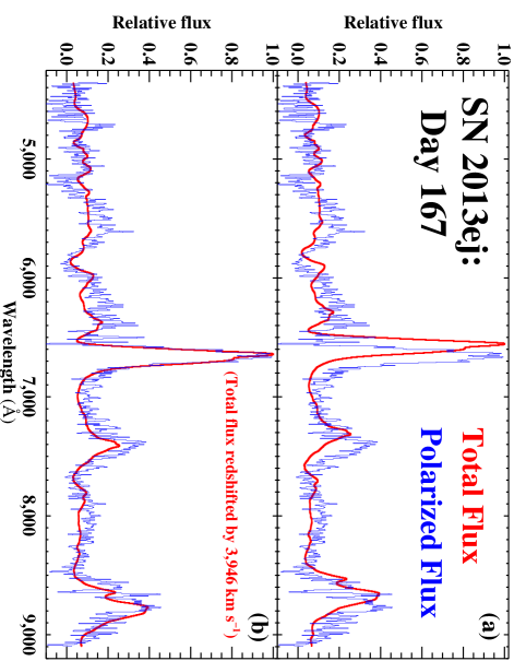
Figure 1: Polarized flux (blue, noisier data) and total flux (red, thick lines) spectra of SN 2013ej, taken 167 days after explosion. The recession velocity of $657$ km s^-1 (Lu et al., 1993) has been removed from these and all data unless otherwise noted. The polarized flux was derived by multiplying the total flux by the observed polarization percentage at each wavelength, where the polarization percentage was estimated through calculation of the rotated Stokes parameter (RSP; see Appendix A.1). (a) Observed data. (b) Same as in (a) but with the total flux spectrum now artificially redshifted by $3,946$ km s^-1. To aid comparison of features, the total flux spectrum was first scaled by a factor of 0.0041 (chosen to produce the best fit to the H$\alpha$ spectral region), and then normalized to unity with the same normalization factor also applied to the polarized flux.

Figure 2: Simplified schematic of physical situation proposed to generate the redshifted polarized flux spectrum seen in SN 2013ej at nebular epochs. The SN flux spectrum is produced interior to an external scatterer that is located within the (homologously) expanding and otherwise transparent nebula that makes up the SN remnant. The scattering source recedes from the center of the nebula with velocity $v_{\rm rec}$ at an angle to the line-of-sight (LOS), chosen here to be $\alpha_{\rm LOS}=90^{\circ}$. This yields a LOS velocity relative to the distant observer of $v_{\rm LOS}=v_{\rm rec}\cos{\alpha_{\rm LOS}}$. Under this arrangement, the portion of the total flux spectrum that is scattered by the source and redirected towards the observer receives both a net polarization and a redshift with respect to the total flux spectrum received directly. The polarization arises from the scattering process (i.e., $p\propto\sin^{2}[\alpha_{\rm LOS}]$, achieving a maximum for $\alpha_{\rm LOS}=90^{\circ}$), while the redshift is imparted according to $v_{\rm shift}=v_{\rm rec}-v_{\rm LOS}=v_{\rm rec}(1-\cos{\alpha_{\rm LOS}})$. Note that for simplicity the SN flux spectrum is depicted here as being generated solely in the innermost part of the ejecta; in reality (and, in our models), line emission occurs through an extended ejecta volume, resulting in some departures from a perfect replication of the total flux in the polarized flux spectrum (see Appendix C.1).

1. The first clear signature of the high-velocity scatterer emerged sometime between days 97 and 134 after explosion. We searched all other epochs of our data (i.e., those from days 8, 34, 55, 67, 97, and 134; see Table A1 in the Appendix) for significant correlation between the total and polarized fluxes by running FXCOR at each epoch in a manner identical to our treatment of the day 167 data. The other nebular-phase epoch, taken on day 134, yielded results very similar to, albeit with somewhat less significance than, those obtained on day 167: A single, strongly peaked correlation at $v_{\rm shift}=4,368\pm 232$ km s^-1, Tonry & Davis $R$ value of 7.6, and a correlation percentage of 84%. None of the earlier, photospheric epochs yielded a Tonry & Davis $R$ value greater than 1.7 or a correlation greater than 34% for any velocity shift (see Table B1 in the Appendix).

2. The total and polarized flux profiles of strong emission lines (i.e., H$\alpha$ $\lambda$6563 Å; [Ca II] $\lambda\lambda$7291, 7324 Å; Ca II $\lambda\lambda$8498, 8542, 8662 Å) are closely matched in terms of breadth and specific spectral characteristics including, notably, asymmetries in the line profiles. We show the data for the H$\alpha$ region in Figure 3 for both nebular epochs.

3. The overall spectral energy distributions (that is, the spectral shapes across the observed range from $4300$ Å — $9100$ Å) of the total and polarized fluxes are the same (Figure 1, and Figure B1 in the Appendix).

Taken in turn, these facts generically imply that the scattering source must (1) have first come to dominate the polarization signal during the early nebular phase of the SN’s development; (2) possess some degree of geometrical confinement and be situated largely external to the region responsible for the bulk of the line emission; and (3) be effectively “gray” (that is, independent of wavelength) in its scattering opacity. This final characteristic argues naturally for free electrons as the scattering agent.

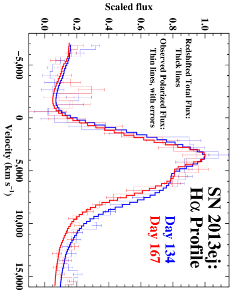
Figure 3: Polarized flux (thin lines, with 1$\sigma$ statistical uncertainties) and total flux (thick lines) spectra across the H$\alpha$ profile of SN 2013ej during the two nebular epochs sampled by our observations. The total flux spectra have been artificially redshifted by $4,368$ km s^-1 (Day 134) and $3,946$ km s^-1 (Day 167), and scaled by factors of 0.0035 (Day 134) and 0.0041 (Day 167), to assist with the direct comparison of features. The peaks of the total flux at both epochs have been normalized to unity, with the same scaling then also applied to the polarized flux. Note that the polarized flux data have a wider binning than the total flux data to improve the SNR.

To test our basic model and draw quantitative conclusions, we performed time-dependent, non-local thermodynamic equilibrium radiative transfer simulations of SN ejecta with CMFGEN coupled to an upgraded version of the 2D polarized radiative transfer code LONG_POL (Dessart et al., 2021b, and references therein). The simulations were carried out in the manner described by Dessart et al. (2021a), but with model x3p0ext4 selected from Hillier & Dessart (2019) for the progenitor and ejecta — a red supergiant (RSG) progenitor of initial mass ${\rm M}_{\rm init}=15\ {\rm M}_{\odot}$ (consistent with the inferred progenitor of SN 2013ej; Dhungana et al. 2016) demonstrated by Hillier & Dessart (2019) to best replicate the photometric and spectroscopic properties of SN 2013ej. We aged the explosion to the epoch of our final observations, and then inserted a region of enhanced free electron density (i.e., density enhancement factor $N_{\rm e,fac}$ relative to the surrounding free-electron density) in the outer ejecta to serve as the scattering source.

Following Dessart et al. (2021a), we ran multiple simulations, allowing $N_{\rm e,fac}$, $v_{\rm rec}$, $\alpha_{\rm LOS}$, and the region’s opening angle (defined as $2\beta$, where $\beta$ is the half-opening angle) and spread in radial velocity ($v_{\rm spread}$) to vary and tested each realization for conformity with observational constraints (Appendix C.2). Redshifted, polarized fluxes showing a clean reflection of the total flux were routinely obtained in our simulations, provided the scattering region had sufficient optical depth and was placed well outside of the primary region of spectrum formation. Figure 4 presents results from one such simulation, together with a direct comparison with the observed polarization for SN 2013ej on day 167. The overall agreement between our models and the observations in terms of both the specific character and the level of the observed polarization demonstrate that our basic ansatz is indeed capable of replicating the essential observations of SN 2013ej.

Figure 4: Comparing models to observations. Results from a 2D polarized radiative transfer simulation described in the text and designed according to the basic physical setup depicted in Figure 2 and detailed by Dessart et al. (2021a). The scattering source in this example is characterized by $v_{\rm rec}=4,000$ km s^-1, $v_{\rm spread}=400$ km s^-1, $\alpha_{\rm LOS}=90^{\circ}$, $2\beta=30^{\circ}$, and $N_{\rm e,fac}=100$. (a, b) Total and polarized flux resulting from the simulation, presented in a manner identical to that shown for the data of SN 2013ej in Figure 1, where we have again normalized all spectra to 1.0 at the location of the H$\alpha$ peak. (c) Direct comparison between the model’s predicted polarization (red, smooth curve) and that actually observed for SN 2013ej on Day 167 (black, noisy data).

Further comparisons between the models and observations permit quantitative constraints on the location and distribution of the scatterer (or, scatterers) to be drawn. First, we note again that the entire emission profiles, including asymmetries, appear well replicated in polarized light (Figures 1 and 3). From the velocity of the blue edges of the emission profiles relative to line center, we are thus able to conservatively set the recession velocity of the inner parts of the scatterer, which typically dominate the redshift imparted to the polarized flux (Dessart et al., 2021a), at $\sim 4,000$ km s^-1. Since $v_{\rm shift}\approx 4,000$ km s^-1 for the observations of SN 2013ej, this effectively limits $\alpha_{\rm LOS}$ to values of $\alpha_{\rm LOS}\lesssim 90^{\circ}$ (Figure 2); that is, the dominant scattering source responsible for the polarization must be located close to the plane of the sky or in the approaching hemisphere of the remnant.

Second, the lack of broadening of the polarized flux profiles of lines relative to the profiles seen in the total flux (Figure 3) constrains the opening angle of the scatterer to values of $2\beta\lesssim 40^{\circ}$, since a less confined scatterer unacceptably broadened the polarized line profile in our models (Appendix C.2). This also restricts any “bi-polar” (or otherwise multiply distributed) arrangement to the scatterer(s) to orientations within $\sim 10^{\circ}$ of the plane of the sky and with nearly identical values of $v_{\rm rec}$ (see Appendix C.2). To summarize: Comparing our models with the observed data constrains a single, asymmetrically distributed scatterer to have $\alpha_{\rm LOS}\lesssim 90^{\circ}$, $v_{\rm rec}>4,000$ km s^-1, and $2\beta<40^{\circ}$; if multiple scatterers are responsible for the polarization, they must all be contained close to the plane defined by $\alpha_{\rm LOS}\approx 90^{\circ}$ (the plane of the sky) and at nearly the same recession velocities.

Establishing the existence of a high-velocity, geometrically confined scatterer does not establish its cause. As discussed in Section 1, a popular scenario capable of producing enhanced free-electron density in the expanding ejecta of CC SNe is decay heating from radioactive nickel, created and ejected during the explosion. To investigate this possibility, we studied the effects of a concentration of ${}^{56}{\rm Ni}$ on the ionization structure of our specific model at nebular times. Consistent with the results of Dessart et al. (2021a), we found that even a relatively small amount ($M_{\rm Ni}\approx 0.004\ {\rm M}_{\odot}$), placed in a very confined clump at sufficient velocity ($v_{\rm rec}\gtrsim 4,000$ km s^-1) produced ionization and, hence, electron density enhancements sufficient to generate the polarization levels observed (e.g., Figure 4).

The enhanced electron density in our simulations typically extended $\gtrsim 500$ km s^-1 beyond the specific location of the nickel clump, into both the denser, more slowly moving ejecta and the less-dense, more quickly moving ejecta. Since it is the recession speed of the inner edge of the enhanced electron density that is typically responsible for the redshift imparted to the polarized flux (Dessart et al., 2021a), this locates the putative ⁵⁶Ni in SN 2013ej at a minimum recession velocity of $\gtrsim 4,500$ km s^-1.

4 Conclusions and Discussion

In this work, we show direct evidence from nebular-phase spectropolarimetry that a confined, asymmetrically distributed, high-velocity scattering source exists in the ejecta of the Type II-P/L SN 2013ej. We find the most plausible physical origin to be free electrons liberated through ionization caused by the decay of radioactive ⁵⁶Ni, synthesized by and launched as part of the explosion with final radial velocity exceeding $4,500$ km s^-1.

This specific finding for SN 2013ej, an otherwise fairly typical CC SN arising from a progenitor star with a massive hydrogen envelope intact (Dhungana et al., 2016; Hillier & Dessart, 2019), must be viewed in light of the predictions of hydrodynamical simulations of neutrino-driven SN explosions. Calculations in such stars that incorporate the development of Rayleigh-Taylor instabilities (Chevalier, 1976), when carried out assuming an initially spherical SN shock, have proven capable of obtaining maximum ${}^{56}{\rm Ni}$ velocities of $\sim 2,000$ km s^-1 (Herant & Benz, 1991). More recently, such models that treat consistently the development of explosion asymmetries — produced by convective instabilities behind the stalled shock and the standing accretion shock instability (Blondin et al., 2003) — have achieved maximum ${}^{56}{\rm Ni}$ velocities of between $3,700-4,400$ km s^-1 in some instances (Wongwathanarat et al., 2015), with speeds approaching $\sim 5,000$ km s^-1 claimed in only the most extreme cases (Orlando et al., 2021).

In this context, it may also be useful to consider studies of the much more energetic SNe associated with long-duration $\gamma$-ray bursts (GRBs), which arise from fast-rotating, higher-mass progenitors (${\rm M_{\rm initial}}\gtrsim 25{\rm\ M}_{\odot}$; Woosley & Bloom 2006) whose envelopes have been completely stripped of their hydrogen and helium layers prior to explosion. Here, detection of extremely high-velocity ($v\gtrsim 100,000$ km s^-1), Ni-rich ejections of material (Izzo et al., 2019) implicate a grossly non-spherical explosion in which the explosion mechanism — typically envisaged as requiring a “central engine” (Sobacchi et al., 2017) — drives material well beyond the denuded core of the progenitor star. Similarly high-velocity material is also inferred from the characteristics of very early time spectra of some “stripped-envelope” CC SNe that are not associated with GRBs (i.e., SNe Ib/c, IIb; Izzo et al. 2020). The confirmation that a high-velocity scatterer exists in the thinning ejecta of SN 2013ej may bolster the contention (see Ono et al. 2020, and references therein) that a related mechanism is at play in more typical SNe II that arise from lower-mass progenitors (Smartt, 2015), with unequivocal polarization signatures only coming to dominate the signal once the thick, initially opaque hydrogen envelope has turned sufficiently transparent. Additional, high SNR nebular-phase spectropolarimetry of nearby Type II SNe are certainly warranted to further test this conjecture.

Appendix A Data Acquisition, Reduction, and Correction for ISP

A.1 Observations and Data Reduction

Our complete observational program gathered seven epochs of spectropolarimetry of SN 2013ej. All observations were made at the VLT with FORS2 mounted at the Cassegrain focus of the Antu (UT1) telescope. The data sample days 8 – 172 following the estimated date of explosion. Details of the observational epochs, instrumental setup, exposure times, and observational conditions are given in Table A1. Note that due to observational constraints (maximum visibility of SN 2013ej of $\sim 1$ hour by the final observations, as it set shortly after sunset), the two nebular-phase epochs (i.e., epochs 6 and 7) that are the focus of this study incorporate data taken on multiple nights. The timing of all of the spectropolarimetric epochs relative to the photometric light curve of SN 2013ej is shown in Figure A1.

The data reduction, including extraction of the spectra, correction for the small ($\lesssim 0.1\%$) amount of instrumental polarization known to exist at the VLT (Cikota et al., 2017), and formation of the Stokes parameters and total flux spectra, was carried out according to the procedures described by Dessart et al. (2021b). From each epoch’s final observed dataset, we subtracted the ISP derived in Appendix A.2, removed a redshift of 657 km s^-1 (Lu et al., 1993, via NED), and rebinned to $5$ Å bin^-1 over a wavelength range of $4300$ Å – $9100$ Å.

Table A1: Journal of Spectropolarimetric Observations of SN 2013ej

				Exposure	Air	Seeing	Slit
Epoch	Day	UT Date	MJD	(s)	Mass	(arcsec)	(arcsec)
1	8.442	2013-08-01.392	56,505.392	5,760 (10)	1.31–1.40	1.0	1.0
2	34.346	2013-08-27.296	56,531.296	3,600 (8)	1.31–1.45	1.0	1.5
3	55.277	2013-09-17.227	56,552.227	3,680 (5)	1.33–1.49	1.0	1.5
4	67.307	2013-09-29.257	56,564.257	6,400 (21)	1.31–1.51	0.8	1.5
5	97.297	2013-10-29.247	56,594.247	7,200 (15)	1.35–2.34	1.2	1.0
6	133.150	2013-12-04.100	56,630.100	9,600 (2)	1.31–1.61	1.7	1.6
$\cdots$	134.144	2013-12-05.094	56,631.094	8,050 (2)	1.31–1.51	1.0	1.6
7	163.106	2014-01-03.056	56,660.056	3,600 (1)	1.43–1.64	1.0	1.0
$\cdots$	164.113	2014-01-04.063	56,661.063	3,600 (2)	1.46–1.76	1.0	1.6
$\cdots$	172.105	2014-01-12.055	56,669.055	3,600 (2)	1.54–1.93	1.0	1.6

Note. — All observations were obtained with VLT-FORS2 using the 300 line/mm grism (“GRIS_300V”) along with the “GG435” order-sorting filter to prevent second-order contamination. This resulted in a useable spectral range of 4300 Å – 9200 Å. Observations made through a 1$\farcs$0 slit delivered a resolution of $\sim 12$ Å ($R\approx 550$ at H$\alpha$), whereas those made through 1$\farcs$5 and 1$\farcs$6 slits delivered resolutions of $\sim 17$ Å and $\sim 18$ Å ($R\approx 350$ at H$\alpha$), respectively, derived from the full width at half maximum (FWHM) of night-sky lines.

Figure A1: V-band light curve of SN 2013ej (filled circles; magnitudes are in the Vega-system) with the timings of the seven epochs of spectropolarimetry (Table A1) indicated by vertical arrows, all relative to the date of explosion estimated by Valenti et al. (2014). The photometric data are taken from the Mount Laguna Supernova Survey (MOLASUS; Khandrika 2016) through day 128, and supplemented with data from Huang et al. (2015) thereafter. Dashed, vertical lines denote the precipitous drop in luminosity that occurs during the transition period between the opaque “photospheric” phase (before $\sim$ day 96 for SN 2013ej) and the increasingly transparent radioactive tail phase (after $\sim$ day 106; Yuan et al., 2016). Note that the $V$-band decline of $\sim 0.87$ mag (Bose et al., 2015) between peak and day 50 after explosion places SN 2013ej close to the boundary established by Faran et al. (2014) that separates “Type II-L” from “Type II-P”; indeed, most authors consider SN 2013ej to be an intermediate, or “transitional”, object (Bose et al., 2015; Dhungana et al., 2016; Morozova et al., 2018), one of a growing number that straddle the defining characteristics of the Type II-P/L categories.

To translate the normalized Stokes $q$ and $u$ parameters into estimates of polarization, $p$, we computed the polarization according to each of the four definitions given by Leonard et al. (2001): “Traditional Polarization” ($p_{\rm trad}$), “Debiased Polarization” ($p_{\rm deb}$), “Optimal Polarization” ($p_{\rm opt}$), and “rotated Stokes parameter” (RSP). As expected for data with a strong, non-zero polarization signal, all four calculations yielded very similar results when applied to the observed data. Following Leonard et al. (2001), we calculated the RSP by first smoothing the polarization angle curve and then rotating the Stokes parameters through the wavelength-dependent angle defined by the smoothed curve. This procedure is designed to place all of the polarization signal in the RSP, which makes it effectively equivalent to $p_{\rm trad}$ in regions where the SNR and polarization are high, but with improved noise characteristics in spectral regions with low polarization levels, which exist in our data following removal of the ISP (see Figure 4c). For both presentation and computational purposes, we therefore adopted the RSP as our best estimate of $p$, including for our calculations of the polarized flux. That is, the polarized flux spectra presented and analyzed in this work were produced by multiplying the RSP by the total flux: ${\rm RSP}(\lambda)\times f(\lambda)$. We note that using any of the other estimates for $p$ had minor impact on the resulting polarized flux, except in spectral regions with very low polarization, in which the RSP is much better behaved and, thus, preferred.

A.2 Interstellar Polarization

To derive the ISP for SN 2013ej, we followed the approach detailed by Dessart et al. (2021b), in which strong, unblended emission features (e.g., regions near the peaks of H$\alpha$ and the Ca II IR triplet) are assumed to completely depolarize all SN light during the optically thick photospheric phase, leaving only the ISP. For multi-epoch data, this should present as fixed, unchanging levels of polarization (and, polarization angle) with time in these spectral regions. Figure A2 displays our data taken during the middle of the photospheric phase of SN 2013ej, on days 34, 55, and 67 after explosion (Table A1). Sharp, consistent depolarizations are indeed seen in the spectral regions near the peaks of the H$\alpha$ and Ca II IR triplet lines in the total flux spectrum (i.e., near $6540$ Å and $8620$ Å, respectively). What is more, while the overall polarization level (and, to a lesser extent, the polarization angle) shows substantial evolution over the 33 days covered by these observations, these specific regions do not, always returning to the same polarization level and angle, regardless of epoch. Such constancy is fully consistent with expectations that the total, unchanging ISP is indicated at these wavelengths during these epochs.

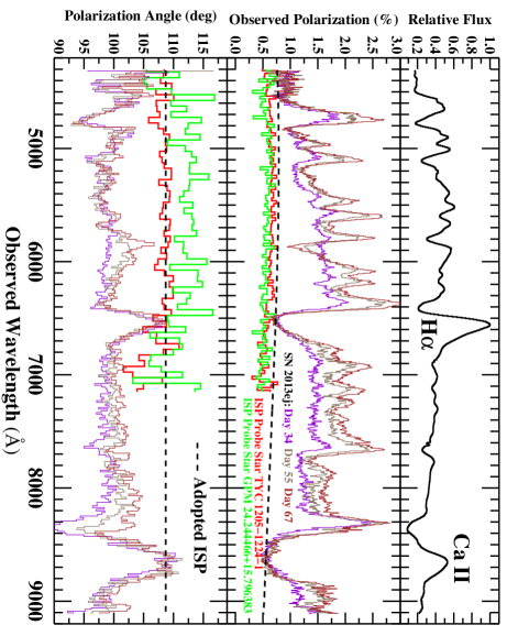
Figure A2: Determining the ISP to SN 2013ej. Top: Total flux spectrum of SN 2013ej taken on day 55 after explosion, with prominent emission lines labeled. Middle: Observed polarization level (thin lines) for three mid-photospheric-phase epochs, color coded by day since explosion (Table A1). Bottom: Same as for middle, but for the observed polarization angle. Also shown in both the middle and bottom panels are the observed polarizations and polarization angles of two Galactic “ISP probe” stars TYC 1205-1224-1 (thick, red lines) and GPM 24.244466+15.796383 (thick, green lines); note that these data do not extend redward of $7150$ Å. The total ISP derived in Appendix A.2 is indicated by the thick, black, dashed line in both panels.

For an SN with minimal extra-Galactic reddening, one way to test any ISP estimate is to observe Galactic “ISP probe” stars (Tran, 1995): Distant, intrinsically unpolarized stars in the Milky Way that lie near to the LOS of the SN and are sufficiently far away to fully probe the ISP produced by Galactic dust. SN 2013ej is an excellent candidate for such a test, since it lacks any detectable interstellar Na I D $\lambda\lambda 5890,5896$ Å absorption at the redshift of its host galaxy (NGC 628) in high-resolution spectra, which implies negligible host-galaxy extinction (Valenti et al., 2014; Bose et al., 2015) and, by logical extension, host-galaxy ISP. We thus obtained spectropolarimetry of two distant Galactic stars using the 6.5 meter Multiple Mirror Telescope (MMT) on Mt. Hopkins on 2016 July 8 (UT), as part of the Supernova Spectropolarimetry (SNSPOL; Hoffman et al. 2017) Project. The data were acquired and reduced as described by Mauerhan et al. (2014). The first “probe” star, GPM 24.244466+15.796383, is separated by only $3\farcm 4$ from SN 2013ej in the sky and is estimated by Gaia parallax (Bailer-Jones et al., 2018) to be $700\pm 30$ pc away. The second star, TYC 1205-1224-1 is separated by $53\farcm 3$, and is estimated by Gaia parallax to be $319\pm 5$ pc away. Both stars satisfy the criterion of Tran (1995) that they be located at least 150 pc above or below the Galactic plane in order to fully sample the Galactic ISP along the LOS. (The Galactic latitude of SN 2013ej, $b=-45.7^{\circ}$, necessitates a distance of at least $210$ pc.)

We overplot the “probe” star spectropolarimetry data in the bottom panel of Figure A2, and find them to show remarkable consistency with expectations based on the depolarized spectral line analysis: The measured polarization levels and polarization angles of both stars are very close to those measured in the H$\alpha$ peak of SN 2013ej during the photospheric epochs. (The limited spectral range precludes such a direct comparison at the location of Ca II.) Small differences may presumably be attributed to either patchy Galactic ISP or a small amount of host galaxy ISP.

With the overall level and angle of the ISP thus convincingly constrained, we proceeded to derive a total ISP to be subtracted from our data as follows. First, we estimated the observed polarization near the peaks of both H$\alpha$ (6520 Å – 6560 Å) and Ca II (8600 Å – 8640 Å) by taking the average values obtained from all three mid-photospheric epochs. Next, we assumed the empirically derived functional form for ISP given by Serkowski (1973):

$$p_{\rm ISP}=p_{\rm max,ISP}\exp[-K_{\rm ISP}\ln^{2}(\lambda_{\rm max,ISP}/\lambda)]$$ (A1)

where $p_{\rm ISP}$ is the percent polarization at a wavelength $\lambda$, $p_{\rm max,ISP}$ is the maximum level of ISP that occurs at $\lambda_{\rm max,ISP}$ , and $K_{\rm ISP}$ is a constant that determines the full width of the linear polarization curve. We arrived at the level and wavelength dependence for the ISP across our full spectral range then by seeking the set of values of $\lambda_{\rm max,ISP},\ p_{\rm max,ISP}$, and $K_{\rm ISP}$ that produced the best-fitting “Serkowski curve” (i.e., Equation A1) to our two ISP points derived from the H$\alpha$ and Ca II regions. Note that rather than adopting an empirical relation between $K_{\rm ISP}$ and $\lambda_{\rm max,ISP}$ (e.g., Cikota et al., 2017), we chose instead to allow $K_{\rm ISP}$ to range between 0.6 and 1.5, based on the ranges seen in recent studies (see Cikota et al., 2018, and references therein); this also provided a much better fit to our data points. Finally, guided by the wavelengths of peak polarization observed for the Galactic probe stars (Figure A2), we restricted $\lambda_{\rm max,ISP}$ to lie between $5,000-5,500$ Å.

Our minimization resulted in best-fit values of $p_{\rm max,ISP}=0.79\%$, $\lambda_{\rm max,ISP}=5100$ Å, and $K_{\rm ISP}=1.28$; we set the polarization angle to be $\theta_{\rm ISP}=108.7^{\circ}$, the simple average of the values obtained over the H$\alpha$ and Ca II regions in our three epochs. This adopted ISP is overplotted in Figure A2, and represents the ISP that was then subtracted from all observed data to produce the intrinsic SN polarization presented and analyzed by this work. The close agreement between the ISP derived from the polarization observed for SN 2013ej itself with that measured from the probe stars, coupled with the evidence for minimal host galaxy ISP, provides confidence in our chosen ISP and the technique used to derive it; small, but justifiable, changes to it were tested and found to have negligible impact on the quantitative results of this work.

We note that our adopted ISP is similar to the ISP value derived by Nagao et al. (2021) in their spectropolarimetric study of SN 2013ej, but differs somewhat from the value chosen by Mauerhan et al. (2017). As pointed out by Nagao et al. (2021), the discrepancy may not be that surprising given that Mauerhan et al. (2017) adopted the ISP derived towards a different SN (SN 2002ap) in the same host galaxy, for which significant host galaxy ISP is suspected (see Nagao et al., 2021, and references therein).

Appendix B Data Analysis

B.1 Deriving the Velocity Shift of the Polarized Flux

To derive the (relativistic) velocity offset between the total and polarized flux spectra, we ran IRAF’s FXCOR task (“Release Mar93”) with the polarized flux spectrum as the “object” and the total flux spectrum as the “template”. We turned on continuum subtraction for both the object and template (not doing so altered the calculated shift by less than 20 km s^-1 in all cases), and ran the correlation over the entire spectral range (4300 – 9100 Å). Following Filippenko et al. (1999), we divided the uncertainty reported by the task by a factor of 2.77, to bring the uncertainties in line with those calculated using equation (20) of Tonry & Davis (1979).

Table B1 presents the results of our cross-correlations for all seven epochs of data. In general, normalized cross-correlation peak values above 0.8 (80% correlation) are considered “excellent”, whereas those below $\sim 0.5$ are not considered to be “good” (Alpaslan, 2009). Significant correlation between the total and polarized flux exists only during the two nebular-phase epochs, on days 134 and 167. For completeness, we show in Figure B1 the data for the day 134 epoch in a manner identical to that shown in Figure 1 for the day 167 data.

From the lack of correlation prior to the nebular phase, our proposed mechanism for the SN polarization — reflection off of an asymmetrically distributed, externally located, high-velocity scatterer — appears to dominate the polarization signal only at nebular times. We have thus focused our analysis here squarely on the nebular data. We note that the photospheric-phase data, some of which are displayed in Figure A2 where they are utilized to derive the ISP, are the same data analyzed by Nagao et al. (2021) in their study of the continuum polarization of SN 2013ej during the photospheric phase. The primary characteristics of the nebular-phase polarization data that are uniquely analyzed by our study — i.e., redshifted, polarized flux observed across all strong line features — are not present at the earlier times investigated by either Nagao et al. (2021) or Mauerhan et al. (2017), and thus demand a distinctly different analysis. We leave an evaluation of the possible contribution that a high-velocity scatterer could have had on the photospheric-phase spectropolarimetry to a future work (D. Leonard et al., in preparation).

Table B1: Measured Correlation Between Total Flux and Polarized Flux

		Normalized Cross-	Peak
Epoch	Day	Correlation Peak	Significance
1	8	0.341	1.6
2	34	0.280	1.7
3	55	0.309	1.5
4	67	0.298	1.3
5	97	0.336	1.5
6	134	0.843	7.6
7	167	0.915	14.6

Figure B1: Comparing the total and polarized flux spectra of SN 2013ej on day 134, displayed as in Figure 1 for the day 167 data. To aid comparison of features, the total flux spectrum has been scaled by a factor of 0.0035, chosen to produce the best fit to the H$\alpha$ spectral region; the total flux spectrum has been artificially redshifted by $4,368$ km s^-1 in (b).

B.2 Constraints on the Broadening of Line Features in the Polarized Flux

For comparison with models (see Appendix C), a critical observational constraint is the degree to which unblended emission-line features appearing in the polarized flux are not broadened relative to the same features in the total flux (Dessart et al., 2021a). Casual examination of Figure 1 and Figure B1 in the Appendix reveals no such obvious broadening. Further, the close agreement between the total and polarized flux line-profile morphologies (Figure 3) convincingly argues in favor of the entire flux profile being reflected rather than a narrower component being broadened by a (finely tuned) spatially extended scatterer.

Assuming this to be the case, we set quantitative limits on any broadening by carrying out the following analysis on the H$\alpha$ profile from the day 167 data. First, we removed the observed velocity shift (i.e., $v_{\rm shift}=3,946$ km s^-1) from the polarized flux. Next, we rebinned both the total and polarized fluxes to the approximate spectral resolution (Table A1), and then converted the wavelength scale to a (relativistic) velocity scale with respect to the rest wavelength of H$\alpha$ (i.e., $6562.8$ Å). We then sought the scaling to apply to the total flux to provide the best match between it and the polarized flux (accounting for uncertainties) over the velocity range of $\pm 5,000$ km s^-1. Minimizing the $\chi^{2}$ of the fit yielded a scaling of $0.0041$, which we then applied to the total flux spectrum. This scaling produced a reduced $\chi^{2}$ of $\chi^{2}_{\rm red}=1.027$ over this velocity range which, for 15 degrees of freedom (i.e., 16 data points and 1 free parameter), implies disagreement between the total and polarized fluxes at the $0.80\sigma$ level for a one-dimensional Gaussian (see discussion by Leonard et al. 2008) — a convincing level of agreement.

We then applied “broadening factors” to the observed polarized flux by multiplying the velocity vector by factors ranging from 0.80 to 1.50, sampling by hundredths. For each realization, we minimized $\chi^{2}_{\rm red}$, keeping the scaling as a free parameter for each fit.

Next, we sought any evidence that the polarized flux was already broadened relative to the total flux, which would logically manifest as better fits for broadening factors of less than unity; no such evidence was found. On the other hand, the fits did slightly improve for broadening factors greater than unity, up through a factor of 1.07 (i.e., a 7% broadening), for which $\chi^{2}_{\rm red}=0.72$. However, given that measurements of $\chi^{2}_{\rm red}$ have an inherent uncertainty of $\sim\sqrt{2/N}$ (Andrae et al., 2010), where N is the number of data points ($N=16$ in this case, resulting in an uncertainty in $\chi^{2}_{\rm red}$ of $\approx 0.35$), the improvement is only significant at the $1\sigma$ level.

To set an upper bound on the possible broadening of the polarized flux we searched for the broadening factor that would yield a $3\sigma$ discrepancy between the total flux and the polarized flux for data characterized by our uncertainties; this occurred at a broadening factor of 1.24. We therefore take a $24\%$ broadening as a conservative upper limit on the possible broadening factor of the polarized flux relative to the total flux that could be present in our data. (Note that this limit gets tighter the higher the SNR of the data: For data with twice the SNR as ours, the limit on the possible broadening factor is only 1.12; for nine times the SNR it is only 1.06.)

Appendix C Modeling and Interpretation

C.1 Theoretical Modeling and Consideration of Dust

The numerical simulations presented by Dessart et al. (2021a) establish that a clump of ${}^{56}{\rm Ni}$ inserted into realistic SN ejecta is capable of generating high enough levels of ionization at nebular times to provide sufficient electron scattering to generate overall polarization at the $\sim 0.5\%$ level seen in our data for SN 2013ej. Here we employed the same code in an effort to: (1) verify the fundamental results of Dessart et al. (2021a) when using a progenitor and ejecta model specific to SN 2013ej; and (2) set quantitative constraints on the distribution of the high-velocity scatterer inferred to exist in its ejecta.

We began with the set of model RSG progenitors presented by Hillier & Dessart (2019), and selected model x3p0ext4 for our direct comparisons since it was shown in that work to most faithfully reproduce the specific light curves and spectral evolution of SN 2013ej itself. To test whether a single, rapidly receding scatterer consisting of enhanced free-electron density could reproduce the polarization observed in the nebular-phase data of SN 2013ej we first aged this model to day 173 and then ran simulations over a wide range of parameter values. Similar to the results of Dessart et al. (2021a), we found the simulations to consistently produce appropriately redshifted, polarized flux spectra, provided the scatterer was placed sufficiently outside (i.e., at velocities $\gtrsim 3,000$ km s^-1; see Figures 8 and 9 of Dessart et al. 2021a) of the primary region of spectrum formation; placing the scatterer at velocities substantially less than this did not replicate the polarized line flux profile of, e.g., H$\alpha$, due to the substantial overlap between the line-emitting and line-scattering regions. We emphasize that our simulations are crafted specifically to investigate the polarization implications of an asymmetrically distributed, high-velocity scattering source. The effects of any asymmetry in the ‘core’ emission region — anticipated to be minor on the nebular-phase polarization but potentially significant for, e.g., line-profile morphology — will be addressed by a future work (L. Dessart et al., in preparation).

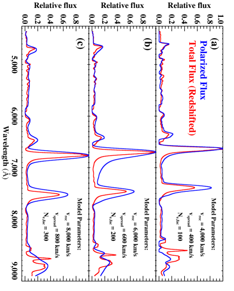
Figure C1: Example total and polarized flux spectra drawn from simulations. Total flux (red) and polarized flux (blue) for three simulations, with the total flux shown in each case artificially redshifted to best match the polarized flux. Each simulation is calculated with the same ejecta structure (RSG model x3p0ext4, from Hillier & Dessart 2019) and age (173 days). All ejecta include a concentration of enhanced free-electron density inserted at $\alpha_{\rm LOS}=90^{\circ}$ (Figure 2) and with opening angle $2\beta=30^{\circ}$, but with differing recession velocities ($v_{\rm rec}$), spreads in radial velocity ($v_{\rm spread}$), and free-electron density enhancements ($N_{\rm e,fac}$), as indicated in each panel. All models yield a polarized flux spectrum appropriately redshifted with respect to the total flux spectrum, and achieve mean polarization levels, calculated over the range 4300 Å $\rightarrow$ 9100 Å, of the same order as that observed in SN 2013ej on day 167: i.e., 0.47%, 0.58%, and 0.20% for the models shown in (a), (b), and (c), respectively, compared with 0.56% measured for SN 2013ej. (Note that a direct comparison between SN 2013ej and the polarization generated by the model depicted here in panel a is shown in Figure 4c.) There is clearly a complex interplay among overall polarization level, breadth of unblended line features in polarized flux (e.g., H$\alpha$), and fidelity of line features seen in polarized flux (particularly evident in the Ca II near-IR lines).

As an example, one realization from our modeling that was found to reasonably replicate both the level and the specific features seen in the polarization of SN 2013ej is shown in Figure 4; Figure C1 shows further examples that provide a sense of how the resulting polarized flux varied with changes in the model’s input parameters (here modifying $v_{\rm rec}$, $v_{\rm spread}$, and $N_{\rm e,fac}$). Degeneracies certainly exist among the model parameters. For instance, models with $\alpha_{\rm LOS}\neq 90^{\circ}$ can achieve quantitatively similar results to those with $\alpha_{\rm LOS}=90^{\circ}$ (i.e., the angle that intrinsically generates maximum polarization and used for the models shown in the figures) with appropriate adjustments to $v_{\rm rec}$ and $N_{\rm e,fac}$; the model presented in Figure 4 is not a unique, “best-fit”. Furthermore, departures from naive expectation based on the simplified toy model presented by Figure 2 are also clearly apparent in both the simulations as well as in the data. For instance, in the model results shown in Figure C1, the polarized flux spectra are not perfect representations of the total flux spectra, deviating notably in the relative strengths and fidelity of specific line features. Similar departures are also seen in the data of SN 2013ej (see Figure 1 and Figure B1 in this Appendix). As discussed by Dessart et al. (2021a), such differences may be expected given that the line emitting region — particularly for the strongest lines — is extended out into the ejecta (and even beyond the region containing the scatterer); it is not the idealized central source depicted in Figure 2.

As also discussed by Dessart et al. (2021a), many of the qualitative results of these simulations could plausibly obtain as well with high-velocity dust serving as the scatterer, since dust is very efficient at scattering, and polarizing, photons. However, a main observational constraint demanded by our observations is wavelength-independence of the scattering source (Section 3) which, while a natural consequence of electron scattering, is not a generic feature of dust scattering unless the grains are much larger than the wavelengths of light being scattered. While no specific studies have yet been carried out that model the wavelength-dependence expected for large-grain dust scattering at optical wavelengths, investigations at longer wavelengths find that the diameters of the smallest grains need to be at least $\sim 3$ times larger than the observed wavelengths to produce “gray” scattering (e.g., Natta et al., 2007). If applied to this situation, it would require grains of at least $\sim 3\ \mu{\rm m}$ in diameter, with little tolerance for any significant contribution by smaller-sized grains.

Such dust would need to be created in the high-velocity, outer ejecta of the SN, most plausibly as the result of interaction between the ejecta and CSM creating a cold, dense shell within which the dust could conceivably form. While there is some observational evidence for early dust formation — sometimes with large ($\gtrsim 1\ \mu{\rm m}$) inferred grain size — in the ejecta of some SNe II (see Priestley et al., 2020, and references therein), the events typically show signs of interaction with a far denser CSM than that inferred to exist in SN 2013ej (Bose et al., 2015; Morozova et al., 2018). Further, the lack of broadening of the polarized flux features (Appendix B.2), as well as their lack of evolution (Section 3), would necessitate a single, persistent dust blob (or two or more such blobs at identical $v_{\rm shift}$), in contrast with basic expectations of dust formed through interaction with a more widely distributed CSM. In contrast, there are clear physical mechanisms that may produce ${}^{56}{\rm Ni}$ clumps or “fingers”, which would naturally yield isolated geometrical entities. Thus, although we can not completely rule out dust as a possibility, we consider it an unlikely agent to explain the specific scattering characteristics that we see here, and have therefore quantitatively pursued free electrons as the scatterer at work in SN 2013ej at these epochs; we postpone to a future study any detailed modeling of dust and its possible impact on the SN radiation, including its possible effect on line profile morphology as well (e.g., Bevan & Barlow, 2016).

C.2 Constraints Derived from the Modeling

Although limited by the degeneracies described in the previous section, our simulations revealed the following three constraining features, which permit us to draw some conclusions about the scattering source at work in SN 2013ej.

1. The scattering that dominates the polarization signal occurs near the inner boundary of the region of enhanced scattering. This is likely due to the dominating contribution to the scattering from the low-velocity portion of the region, where free electron densities are necessarily higher for a given value of $N_{\rm e,fac}$. The amount of the measured difference between $v_{\rm rec}$ and $v_{\rm shift}$ was typically $\sim 500$ km s^-1 (see Figure 4) for free-electron distributions with $v_{\rm spread}=1,000$ km s^-1, the value typically obtained for ionization produced by a confined mass of ⁵⁶Ni in our simulations. This thus requires the actual velocity of the putative ⁵⁶Ni to be at a somewhat larger value than that indicated by the observed velocity shift of the polarized flux alone. Since our observations of SN 2013ej indicate $v_{\rm shift}\approx 4,000$ km s^-1, and the full-profile reflection demands that $v_{\rm rec}\gtrsim 4,000$ km s^-1, this necessarily restricts $\alpha_{\rm LOS}$ to values $\lesssim 90^{\circ}$ (i.e., since $v_{\rm shift}=v_{\rm rec}[1-\cos{\alpha_{\rm LOS}}]$; see Figure 2), and places the putative ⁵⁶Ni in SN 2013ej at a minimum velocity of $\gtrsim 4,500$ km s^-1(i.e., for $\alpha_{\rm LOS}=90^{\circ}$).

   We note here that such a “high velocity” for the scatterer does not introduce a significant time-delay for the reflected spectrum relative to the one that is directly observed. For instance, a scatterer characterized by $v_{\rm rec}=4,500$ km s^-1 would be located on day 167 roughly $2.5$ light-days from the center of the nebula. For $\alpha_{\rm LOS}=90^{\circ}$, the time delay would thus be $\sim 2.5$ days; the maximum possible delay time of $\sim 5$ days would result for $\alpha_{\rm LOS}=180^{\circ}$. During the nebular phase, SN spectra evolve very slowly, and so a few days of delay has negligible impact on the spectrum of the reflected light relative to that received directly.

2. For a single external scatterer, the breadth of unblended line features in polarized flux is driven most strongly by the opening angle, with larger values serving to increase the breadth of the line. In Appendix B.2, we derived the absolute upper limit on the broadening of the H$\alpha$ line in the day 167 polarized flux spectrum of SN 2013ej to be 24%. From our models, any opening angle $\gtrsim 40^{\circ}$ for the scatterer yielded more than this amount of broadening in the polarized flux, thus placing an upper limit of $2\beta\lesssim 40^{\circ}$ on the external scatterer present in SN 2013ej.

3. A bi-polar distribution of identical high-velocity scatterers is only consistent with the data for a narrow range of orientations. We also investigated the effect of multiple scatterers by performing simulations with a “bi-polar” distribution of identical clumps — i.e., two clumps $180^{\circ}$ apart, a popular set-up for jet-like explosion mechanisms (Utrobin & Chugai, 2017; Izzo et al., 2019). Similar to the results of Dessart et al. (2021a), we found that LOS angles of $\alpha_{\rm LOS}\lesssim 60^{\circ}$ (for the approaching clump) produced a clear “double peaked” profile in the polarized flux, decidedly inconsistent with observations of SN 2013ej. Angles between $60^{\circ}\lesssim\alpha_{\rm LOS}\lesssim 80^{\circ}$ produced line profiles which, while no longer double-peaked, were still unacceptably broadened relative to the constraints set on SN 2013ej. From this, we conclude that if a bi-polar distribution of identical scatterers is present in SN 2013ej, it is limited to inclinations within $\sim 10^{\circ}$ of the plane of the sky (i.e., $80^{\circ}\lesssim\alpha_{\rm LOS}\lesssim 100^{\circ}$).

References

- Alpaslan (2009) Alpaslan, M. 2009, arXiv e-prints, arXiv:0912.4755. https://arxiv.org/abs/0912.4755
- Andrae et al. (2010) Andrae, R., Schulze-Hartung, T., & Melchior, P. 2010, arXiv e-prints, arXiv:1012.3754. https://arxiv.org/abs/1012.3754
- Antonucci & Miller (1985) Antonucci, R. R. J., & Miller, J. S. 1985, ApJ, 297, 621, doi: 10.1086/163559
- Appenzeller et al. (1998) Appenzeller, I., Fricke, K., Fürtig, W. et al. 1998, The Messenger, 94, 1
- Bailer-Jones et al. (2018) Bailer-Jones, C. A. L., Rybizki, J., Fouesneau, M., Mantelet, G., & Andrae, R. 2018, AJ, 156, 58, doi: 10.3847/1538-3881/aacb21
- Bevan & Barlow (2016) Bevan, A., & Barlow, M. J. 2016, MNRAS, 456, 1269, doi: 10.1093/mnras/stv2651
- Blondin et al. (2003) Blondin, J. M., Mezzacappa, A., & DeMarino, C. 2003, ApJ, 584, 971, doi: 10.1086/345812
- Bose et al. (2015) Bose, S., Sutaria, F., Kumar, B., et al. 2015, ApJ, 806, 160, doi: 10.1088/0004-637X/806/2/160
- Chevalier (1976) Chevalier, R. A. 1976, ApJ, 207, 872, doi: 10.1086/154557
- Cikota et al. (2017) Cikota, A., Patat, F., Cikota, S., & Faran, T. 2017, MNRAS, 464, 4146, doi: 10.1093/mnras/stw2545
- Cikota et al. (2018) Cikota, A., Hoang, T., Taubenberger, S., et al. 2018, A&A, 615, A42, doi: 10.1051/0004-6361/201731395
- Dessart et al. (2021a) Dessart, L., John Hillier, D., & Leonard, D. C. 2021a, A&A, 651, A10, doi: 10.1051/0004-6361/202140409
- Dessart et al. (2021b) Dessart, L., Leonard, D. C., John Hillier, D., & Pignata, G. 2021b, A&A, 651, A19, doi: 10.1051/0004-6361/202140281
- Dhungana et al. (2016) Dhungana, G., Kehoe, R., Vinko, J., et al. 2016, ApJ, 822, 6, doi: 10.3847/0004-637X/822/1/6
- Faran et al. (2014) Faran, T., Poznanski, D., Filippenko, A. V., et al. 2014, MNRAS, 445, 554, doi: 10.1093/mnras/stu1760
- Filippenko et al. (1999) Filippenko, A. V., Leonard, D. C., Matheson, T., et al. 1999, PASP, 111, 969
- Herant & Benz (1991) Herant, M., & Benz, W. 1991, ApJ, 370, L81, doi: 10.1086/185982
- Hillier & Dessart (2019) Hillier, D. J., & Dessart, L. 2019, A&A, 631, A8, doi: 10.1051/0004-6361/201935100
- Hoffman et al. (2017) Hoffman, J. L., Williams, G. G., Leonard, D. C., et al. 2017, in IAU Symposium, Vol. 329, The Lives and Death-Throes of Massive Stars, ed. J. J. Eldridge, J. C. Bray, L. A. S. McClelland, & L. Xiao, 54–58, doi: 10.1017/S1743921317003052
- Hough (2006) Hough, J. 2006, Astronomy and Geophysics, 47, 3.31, doi: 10.1111/j.1468-4004.2006.47331.x
- Huang et al. (2015) Huang, F., Wang, X., Zhang, J., et al. 2015, ApJ, 807, 59, doi: 10.1088/0004-637X/807/1/59
- Izzo et al. (2020) Izzo, L., Auchettl, K., Hjorth, J., et al. 2020, A&A, 639, L11, doi: 10.1051/0004-6361/202038152
- Izzo et al. (2019) Izzo, L., de Ugarte Postigo, A., Maeda, K., et al. 2019, Nature, 565, 324, doi: 10.1038/s41586-018-0826-3
- Jeffery (2004) Jeffery, D. J. 2004, arXiv e-prints, astro. https://arxiv.org/abs/astro-ph/0406440
- Kawabata et al. (2002) Kawabata, K. S., Jeffery, D. J., Iye, M., et al. 2002, ApJ, 580, L39
- Khandrika (2016) Khandrika, H. G. 2016, Master’s thesis, San Diego State University
- Leonard et al. (2001) Leonard, D. C., Filippenko, A. V., Ardila, D. R., & Brotherton, M. S. 2001, ApJ, 553, 861, doi: 10.1086/320959
- Leonard et al. (2008) Leonard, D. C., Gal-Yam, A., Fox, D. B., et al. 2008, PASP, 120, 1259, doi: 10.1086/595797
- Lu et al. (1993) Lu, N. Y., Hoffman, G. L., Groff, T., Roos, T., & Lamphier, C. 1993, ApJS, 88, 383, doi: 10.1086/191826
- Mauerhan et al. (2014) Mauerhan, J., Williams, G. G., Smith, N., et al. 2014, MNRAS, 442, 1166, doi: 10.1093/mnras/stu730
- Mauerhan et al. (2017) Mauerhan, J. C., Van Dyk, S. D., Johansson, J., et al. 2017, ApJ, 834, 118, doi: 10.3847/1538-4357/834/2/118
- Morozova et al. (2018) Morozova, V., Piro, A. L., & Valenti, S. 2018, ApJ, 858, 15, doi: 10.3847/1538-4357/aab9a6
- Nagao et al. (2019) Nagao, T., Cikota, A., Patat, F., et al. 2019, MNRAS, 489, L69, doi: 10.1093/mnrasl/slz119
- Nagao et al. (2021) Nagao, T., Patat, F., Taubenberger, S., et al. 2021, MNRAS, 505, 3664, doi: 10.1093/mnras/stab1582
- Natta et al. (2007) Natta, A., Testi, L., Calvet, N., et al. 2007, in Protostars and Planets V, ed. B. Reipurth, D. Jewitt, & K. Keil, 767. https://arxiv.org/abs/astro-ph/0602041
- Ono et al. (2020) Ono, M., Nagataki, S., Ferrand, G., et al. 2020, ApJ, 888, 111, doi: 10.3847/1538-4357/ab5dba
- Orlando et al. (2021) Orlando, S., Wongwathanarat, A., Janka, H. T., et al. 2021, A&A, 645, A66, doi: 10.1051/0004-6361/202039335
- Priestley et al. (2020) Priestley, F. D., Bevan, A., Barlow, M. J., & De Looze, I. 2020, MNRAS, 497, 2227, doi: 10.1093/mnras/staa2121
- Serkowski (1973) Serkowski, K. 1973, in IAU Symposium, Vol. 52, Interstellar Dust and Related Topics, ed. J. M. Greenberg & H. C. van de Hulst, 145
- Shapiro & Sutherland (1982) Shapiro, P. R., & Sutherland, P. G. 1982, ApJ, 263, 902, doi: 10.1086/160559
- Silverman et al. (2017) Silverman, J. M., Pickett, S., Wheeler, J. C., et al. 2017, MNRAS, 467, 369, doi: 10.1093/mnras/stx058
- Smartt (2015) Smartt, S. J. 2015, PASA, 32, e016, doi: 10.1017/pasa.2015.17
- Sobacchi et al. (2017) Sobacchi, E., Granot, J., Bromberg, O., & Sormani, M. C. 2017, MNRAS, 472, 616, doi: 10.1093/mnras/stx2083
- Tonry & Davis (1979) Tonry, J., & Davis, M. 1979, AJ, 84, 1511, doi: 10.1086/112569
- Tran (1995) Tran, H. D. 1995, ApJ, 440, 565
- Utrobin & Chugai (2017) Utrobin, V. P., & Chugai, N. N. 2017, MNRAS, 472, 5004, doi: 10.1093/mnras/stx2415
- Valenti et al. (2014) Valenti, S., Sand, D., Pastorello, A., et al. 2014, MNRAS, 438, L101, doi: 10.1093/mnrasl/slt171
- Wongwathanarat et al. (2015) Wongwathanarat, A., Müller, E., & Janka, H. T. 2015, A&A, 577, A48, doi: 10.1051/0004-6361/201425025
- Woosley & Bloom (2006) Woosley, S. E., & Bloom, J. S. 2006, ARA&A, 44, 507, doi: 10.1146/annurev.astro.43.072103.150558
- Yuan et al. (2016) Yuan, F., Jerkstrand, A., Valenti, S., et al. 2016, MNRAS, 461, 2003, doi: 10.1093/mnras/stw1419