Principled Representation Learning for Entity Alignment

Abstract.

Embedding-based entity alignment (EEA) has recently received great attention. Despite significant performance improvement, few efforts have been paid to facilitate understanding of EEA methods. Most existing studies rest on the assumption that a small number of pre-aligned entities can serve as anchors connecting the embedding spaces of two KGs. Nevertheless, no one investigates the rationality of such an assumption. To fill the research gap, we define a typical paradigm abstracted from existing EEA methods and analyze how the embedding discrepancy between two potentially aligned entities is implicitly bounded by a predefined margin in the scoring function. Further, we find that such a bound cannot guarantee to be tight enough for alignment learning. We mitigate this problem by proposing a new approach, named NeoEA, to explicitly learn KG-invariant and principled entity embeddings. In this sense, an EEA model not only pursues the closeness of aligned entities based on geometric distance, but also aligns the neural ontologies of two KGs by eliminating the discrepancy in embedding distribution and underlying ontology knowledge. Our experiments demonstrate consistent and significant improvement in performance against the best-performing EEA methods.

1. Introduction

Knowledge graphs (KGs), such as DBpedia (Auer et al., 2007) and Wikidata (Vrandečić and Krötzsch, 2014), have become crucial resources for many AI applications. Although a large-scale KG offers structured knowledge derived from millions of facts in the real world, it is still incomplete by nature, and the downstream applications are always demanding more knowledge. Entity alignment (EA) is then proposed to solve this issue, which exploits the potentially aligned entities among different KGs to facilitate knowledge fusion and exchange.

Recently, embedding-based entity alignment (EEA) methods (Chen et al., 2017; Sun et al., 2017; Zhu et al., 2017; Wang et al., 2018b; Guo et al., 2019; Ye et al., 2019; Wu et al., 2019; Sun et al., 2020a; Fey et al., 2020) have been prevailing in the EA area. The central idea is to encode entity/relation semantics into embeddings and estimate entity similarity based on their embedding distance. These methods either learn an alignment function $f_{a}$ to minimize the distance between the embeddings of a pair of aligned entities (Wang et al., 2018b), or directly map these two entities to one vector representation (Sun et al., 2017). Meanwhile, they leverage a shared scoring function $f_{s}$ to encode semantics into representations, such that two potentially aligned entities shall have similar feature expression. During this process, a small number of aligned entity pairs (a.k.a., seed alignment) are required as supervision data to align (or merge) the embedding spaces of two KGs.

Different from the conventional laborious methods (Suchanek et al., 2012; El-Roby and Aboulnaga, 2015; Lacoste-Julien et al., 2013) which manually collect and select discriminative features, EEA ones rarely rely on third-party tools or pipeline for preprocessing. Commonly, they just need triples or adjacency matrices of KGs as the input data, and have achieved comparable or better performance on many benchmarks (Sun et al., 2017; Sun et al., 2018; Sun et al., 2020b).

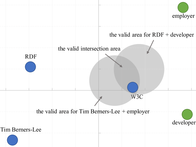
Figure 1. Illustration of margin-based score function. Blue and green nodes denote entity embeddings and relation embeddings, respectively. The center of each grey circle is assigned according to the head entity and relation in the triple. The radii are exactly the margin $\lambda$.

Another strength of EEA is that it suffers slightly from the heterogeneity of two KGs. The relationships among entities are interpreted by the score function $f_{s}$ and manifested as distances in the embedding space. Hence, the similarity between a pair of entities can be defined and estimated smoothly. Without loss of generality, we consider the score function of TransE (Bordes et al., 2013) as $f_{s}$. It describes a triple $(e_{i},r,e_{j})$ by ${\mathbf{e}}_{i}+{\mathbf{r}}\approx{\mathbf{e}}_{j}$, where $e_{i},r,e_{j}$ are the head entity, relation, and tail entity, respectively. The approximation is achieved by defining a margin $\lambda$ to ensure:

(1) $$||{\mathbf{e}}_{i}+{\mathbf{r}}-{\mathbf{e}}_{j}||\leq\lambda,$$

where $||\cdot||$ denotes the L1 or L2 distance. We illustrate this concept in Figure 1, where the two triples (Tim Berners-Lee, employer, W3C) and (RDF, developer, W3C) have the same tail entity W3C. The valid area for W3C is decided by two circles. Their centers are $\textit{Tim Berners-Lee}+\textit{employer}$ and $\textit{RDF}+\textit{developer}$, respectively. The radii are exactly the margin $\lambda$. Therefore, the desired embedding of W3C should be located in the intersection area.

Many existing EEA methods (Chen et al., 2017; Sun et al., 2017; Sun et al., 2018) have explored how to choose a proper $\lambda$ for the entity alignment task, but we argue this goes beyond a mere parameter-tuning problem. In this paper, we define a paradigm leveraged by the current methods. We show that the embedding discrepancy of an underlying aligned entity pair is bounded by $\epsilon\propto\lambda$, for most EEA methods (Chen et al., 2017; Sun et al., 2017; Zhu et al., 2017; Sun et al., 2018; Pei et al., 2019b), or allowing more divergence between two potentially aligned entities (Wang et al., 2018b; Guo et al., 2019; Wu et al., 2019; Ye et al., 2019; Sun et al., 2020a). Further, we find that this margin-based bound cannot be set as tight as expected, causing minimal constraints on the entities with few neighbors. Take W3C in Figure 1 as an example. The valid area will shrink and finally disappear if this entity has more and more linked neighbors. There is only one way to mitigate this problem – enlarging the radii, which will allow more divergence for entities with a few neighbors.

We consider additional constraints on entity embeddings to mitigate the above problem, which we name neural-ontology-driven entity alignment (abbr., NeoEA). An ontology (Horrocks et al., 2006; Grau et al., 2008; Baader et al., 2005) is usually comprised of axioms that define the legitimate relationships among entities and relations. Those axioms make a KG principled (i.e., constrained by rules). For example, an “Object Property Domain” axiom in OWL 2 EL (Grau et al., 2008) claims the valid head entities for a specific relation (e.g., the head entities of relation “birthPlace” should be in class “Person”), and it thus determines the head entity distributions of this relation. The neural ontology in this paper is reversely deduced from the entity embedding distributions, which is clearly different from the existing methods like OWL2Vec* (Chen et al., 2021) that leverages external ontology data to improve KG embeddings. We expect to align the high-level neural ontologies to diminish the discrepancy of entity embedding distributions and ontology knowledge between two KGs.

The main contributions of this paper are threefold:

• We define a paradigm for the current EEA methods, and demonstrate that the margin $\lambda$ in their scoring function $f_{s}$ implicitly bounds the embedding discrepancy in each potential alignment pair. We show that this margin-based bound cannot be as tight as we expect.

• We propose NeoEA to learn KG-invariant and principled representations by aligning the neural axioms of two KGs. We prove that minimizing the difference can substantially align their corresponding ontology-level knowledge without assuming the existence of real ontology data.

• We conducted experiments to verify the effectiveness of NeoEA with several state-of-the-art methods as baselines. We show that NeoEA can consistently and significantly improve their performance.

2. Background

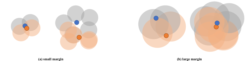
Figure 2. Influence of margin $\lambda$ to different entities in EEA. Blue and orange nodes denote the entities in ${\mathcal{E}}_{1}$ and ${\mathcal{E}}_{2}$, respectively.

2.1. Embedding-based Entity Alignment

We start by defining a typical KG ${\mathcal{G}}=({\mathcal{E}},{\mathcal{R}},{\mathcal{T}})$, where ${\mathcal{E}}$ and ${\mathcal{R}}$ are the entity and relation sets respectively, and ${\mathcal{T}}\subseteq{\mathcal{E}}\times{\mathcal{R}}\times{\mathcal{E}}$ is the triple set. A triple $(e_{1},r,e_{2})$ comprises three elements, i.e., the head entity $e_{1}$, the relation $r$, and the tail entity $e_{2}$. We use the boldface ${\mathbf{e}}_{1}$ to denote the embedding of the entity $e_{1}$.

The common paradigm employed by most existing EEA methods (Chen et al., 2017; Sun et al., 2017; Zhu et al., 2017; Sun et al., 2018; Pei et al., 2019b) is then defined as:

Definition 0 (Embedding-based Entity Alignment).

The input of EEA is two KGs ${\mathcal{G}}_{1}=({\mathcal{E}}_{1},{\mathcal{R}}_{1},{\mathcal{T}}_{1})$, ${\mathcal{G}}_{2}=({\mathcal{E}}_{2},{\mathcal{R}}_{2},{\mathcal{T}}_{2})$, and a small subset of aligned entity pairs $\mathcal{S}\subset\mathcal{E}_{1}\times\mathcal{E}_{2}$ as seeds to connect ${\mathcal{G}}_{1}$ with ${\mathcal{G}}_{2}$. An EEA model consists of two neural functions: an alignment function $f_{a}$, which is used to regularize the embeddings of pairwise entities in ${\mathcal{S}}$; and a scoring function $f_{s}$, which scores the embeddings based on the joint triple set ${\mathcal{T}}_{1}\cup{\mathcal{T}}_{2}$. EEA estimates the alignment of an arbitrary entity pair $(e_{i}^{1},e_{j}^{2})$ by their geometric distance $d({\mathbf{e}}_{i}^{1},{\mathbf{e}}_{j}^{2})$.

The existing studies have explored a diversity of $f_{a}$. The pioneering work MTransE (Chen et al., 2017) was proposed to learn a mapping matrix to cast an entity embedding ${\mathbf{e}}_{i}^{1}$ to the vector space of ${\mathcal{G}}_{2}$. SEA (Pei et al., 2019b) and OTEA (Pei et al., 2019a) extended this approach with adversarial training to learn the projection matrix. Especially, OTEA is highly related to our approach as it is also based on optimal transport (OT) (Arjovsky et al., 2017). The differences are: (1) NeoEA provides a general way to align entity embedding distributions, while OTEA regularizes the projection matrix via optimal transport. (2) NeoEA exploits the underlying ontology information to facilitate entity alignment.

Recently, a simpler yet more efficient method was widely-used, which directly maps a pair of aligned entities $(e_{i}^{1},e_{i}^{2})\in{\mathcal{S}}$ to one embedding vector ${\mathbf{e}}_{i}$ (Sun et al., 2017; Zhu et al., 2017; Guo et al., 2019). Meanwhile, some methods (Wang et al., 2018b; Pei et al., 2019b; Wu et al., 2019) started to leverage a softer way to incorporate seed information, in which the distance between entities in a positive pair (i.e., known alignment in $\mathcal{S}$) is minimized, while that referred to a negative pair is enlarged. As the most efficient choice, we consider $f_{a}$ as Euclidean distance between two embeddings (Sun et al., 2020a; Guo et al., 2019; Wang et al., 2018b; Pei et al., 2019b; Wu et al., 2019). The corresponding alignment loss can be written as follows:

(2) $$\begin{split}\mathcal{L}_{a}=&\sum_{(e_{i}^{1},e_{i}^{2})\in\mathcal{S}}||{\mathbf{e}}_{i}^{1}-{\mathbf{e}}_{i}^{2}||+\sum_{(e_{i^{\prime}}^{1},e_{j^{\prime}}^{2})\in\mathcal{S}^{-}}\mathit{ReLU}(\alpha-||{\mathbf{e}}_{i^{\prime}}^{1}-{\mathbf{e}}_{j^{\prime}}^{2}||),\end{split}$$

where $\mathcal{S}^{-}$ denotes the set of negative pairs. $\alpha$ is the minimal margin allowed between entities in each negative entity pair.

On the other hand, the scoring function $f_{s}$ also has various design choices (Sun et al., 2017; Guo et al., 2019; Wang et al., 2018b). Most methods (Chen et al., 2017; Sun et al., 2017; Pei et al., 2019b, a; Sun et al., 2018) choose TransE as their scoring function, i.e., $f_{s}(\tau)=f_{s}((e_{i},r,e_{j}))=||{\mathbf{e}}_{i}+{\mathbf{r}}-{\mathbf{e}}_{j}||,\tau=(e_{i},r,e_{j})\in{\mathcal{T}}_{1}\cup{\mathcal{T}}_{2}$. The corresponding loss is:

(3) $$\begin{split}\mathcal{L}_{s}=&\sum_{\tau\in{\mathcal{T}}_{1}\cup{\mathcal{T}}_{2}}\mathit{ReLU}(f_{s}(\tau)-\lambda)+\sum_{\tau^{\prime}\in{\mathcal{T}}_{1}^{-}\cup{\mathcal{T}}_{2}^{-}}\mathit{ReLU}(\lambda-f_{s}(\tau^{\prime})),\end{split}$$

where ${\mathcal{T}}_{1}^{-}$ and ${\mathcal{T}}_{2}^{-}$ are negative triple sets. $\mathcal{L}_{s}$ is a margin-based loss in which the distance $d({\mathbf{e}}_{i}+{\mathbf{r}},{\mathbf{e}}_{j})$ in a positive triple should at least be smaller than $\lambda\geq 0$, while larger than $\lambda$ for negative ones.

2.2. Understanding and Rethinking EEA

We illustrate how an EEA method works with Figure 2. When the KG embedding model has a small margin, as shown in the left of Figure 2a, the entities with few neighbors can be constrained tightly. With aligned entity pairs serving as anchors, the circles are very close to each other. Therefore, two entities stay closely in the overlapped intersection areas. By contrast, there is no valid area for the entities with rich neighbors. The entities in the right of Figure 2a are not “fully expressed” (Kazemi and Poole, 2018; Trouillon et al., 2016).

If we enlarge the margin, as shown in Figure 2b, the embeddings for entities with rich neighbors can be correctly assigned. However, the intersection areas for entities with few neighbors are too loose to bound the underlying aligned entities. The two embeddings are not as similar as we expect in the vector space. We summarize the above observations as:

Proposition 0 (Discrepancy Bound).

The embedding difference of two potentially aligned entities $(e_{x}^{1},e_{y}^{2})$ is bound by $\epsilon$, which is proportional to the hyper-parameter $\lambda$:

(4) $$\exists\epsilon\propto\lambda,||{\mathbf{e}}_{x}^{1}-{\mathbf{e}}_{y}^{2}||\leq\epsilon.$$

Proof.

We start with the case that each entity in $(e_{x}^{1},e_{y}^{2})$ has only one neighbor, connected by the same relation $r^{1}=r^{2}$. We assume that their neighbors are actually a pair of aligned entities $(e_{i}^{1},e_{i}^{2})\in{\mathcal{S}}$. With a well-trained and almost optimal EEA model, we have ${\mathbf{e}}_{i}^{1}={\mathbf{e}}_{i}^{2}$ (as $\mathcal{L}_{a}$ is minimized) and ${\mathbf{r}}^{1}={\mathbf{r}}^{2}$ (denoted by ${\mathbf{r}}$ for simplicity). According to Equation (3), we have:

(5) $$||f_{s}({\mathbf{e}}_{x}^{1},{\mathbf{r}},{\mathbf{e}}_{i}^{1})||\approx||f_{s}({\mathbf{e}}_{y}^{2},{\mathbf{r}},{\mathbf{e}}_{i}^{2})||\leq\lambda.$$

Without loss of generality, we consider the scoring function of TransE as $f_{s}$, and then derive:

(6) $$||{\mathbf{e}}_{x}^{1}+{\mathbf{r}}-{\mathbf{e}}_{i}^{1}||\leq\lambda,\quad||{\mathbf{e}}_{y}^{2}+{\mathbf{r}}-{\mathbf{e}}_{i}^{2}||\leq\lambda.$$

For simplicity, we use a constant $C$ to denote ${\mathbf{r}}-{\mathbf{e}}_{i}^{1}$ and ${\mathbf{r}}-{\mathbf{e}}_{i}^{2}$, such that Equation (6) will be rewritten as

(7) $$||{\mathbf{e}}_{x}^{1}+C||\leq\lambda,\quad||{\mathbf{e}}_{y}^{2}+C||\leq\lambda.$$

Then, we get

$$2\lambda\geq ||{\mathbf{e}}_{x}^{1}+C||+||{\mathbf{e}}_{y}^{2}+C||$$

$$\geq ||({\mathbf{e}}_{x}^{1}+C)-({\mathbf{e}}_{y}^{2}+C)||$$

(8) $$= ||{\mathbf{e}}_{x}^{1}-{\mathbf{e}}_{y}^{2}||.$$

Now, we consider a more complicated case, where the neighbors of $e_{x}^{1}$ and $e_{y}^{2}$ are not in the known alignment set. We denote ${\mathbf{r}}-{\mathbf{e}}_{i}^{1}$ and ${\mathbf{r}}-{\mathbf{e}}_{i}^{2}$ by $C^{1}_{i}$ and $C^{2}_{i}$, respectively. If the neighbors of the neighbors $e_{i}^{1},e_{i}^{2}$ are a pair of known alignment, we will have $||C^{1}_{i}-C^{2}_{i}||=||{\mathbf{e}}_{i}^{2}-{\mathbf{e}}_{i}^{1}||\leq 2\lambda$, otherwise we can recursively navigate more neighbors. Therefore, we have:

$$2\lambda\geq ||{\mathbf{e}}_{x}^{1}-{\mathbf{e}}_{y}^{2}+(C^{1}_{i}-C^{2}_{i})||$$

(9) $$\geq ||{\mathbf{e}}_{x}^{1}-{\mathbf{e}}_{y}^{2}||-||C^{1}_{i}-C^{2}_{i}||,$$

which results to an looser bound:

(10) $$||{\mathbf{e}}_{x}^{1}-{\mathbf{e}}_{y}^{2}||\leq 2\lambda+||C^{1}_{i}-C^{2}_{i}||.$$

For the case that the entities $(e_{x}^{1},e_{y}^{2})$ have more than one neighbors, the bound will be further tighten as the embeddings are constrained by multiple triples. ∎

Proposition 2 suggests that decreasing the value of $\lambda$ will decrease the embedding discrepancy in the underlying aligned entity pairs. However, previous studies (Trouillon et al., 2016; Kazemi and Poole, 2018) have proved that $\lambda$ cannot be set as small as we want. This is because TransE with a small margin is not sufficient to fully capture the semantics contained in triples. Some empirical statistics (Sun et al., 2018) also illustrate such results. Enlarging the margin $\lambda$, on the other hand, will bring significant variance between ${\mathbf{e}}_{x}^{1}$ and ${\mathbf{e}}_{y}^{2}$, especially for those entities with few neighbors. For the models that do not belong to the TransE family, e.g., neural-based like ConvE (Dettmers et al., 2018), or composition-based like ComplEx (Trouillon et al., 2016), as proved in  (Wang et al., 2018a; Kazemi and Poole, 2018), they are more expressive than TransE. In this case, entities with sufficient neighbors can be correctly modeled, while entities with only a few neighbors are also less constrained. Therefore, those models allow more diversity between ${\mathbf{e}}_{x}^{1}$ and ${\mathbf{e}}_{y}^{2}$. We believe this is why they performed badly in the EA task (Guo et al., 2019; Sun et al., 2020b).

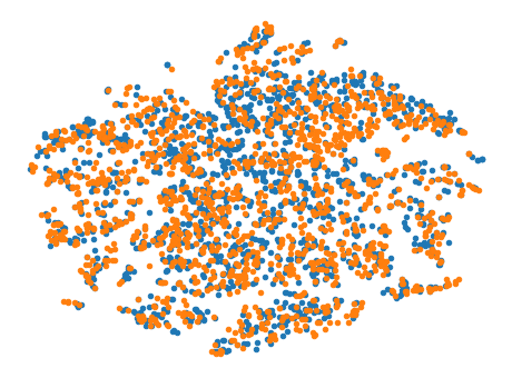
(a)

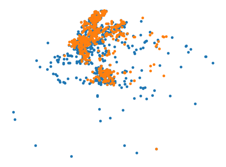
(b)

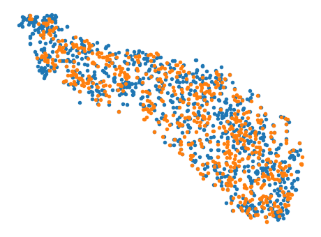
(c)

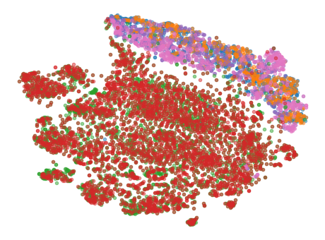
(d)

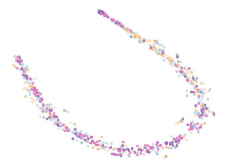
(e)

Figure 3. Example of different embedding distributions. (a) Entity embedding distributions of two KGs, i.e., ${\mathbb{A}}_{E}$. $Blue$ points denote entities in ${\mathcal{G}}_{1}$, and $orange$ ones are entities in ${\mathcal{G}}_{2}$. The two embedding sets are nearly uniformly distributed and almost aligned (based on the EEA model RDGCN (Wu et al., 2019), the same below). (b) The head entity embedding distributions of relation “genre”. The two distributions are only aligned partially. (c) Head entity embedding distributions conditioned on “genre”, i.e., ${\mathbb{A}}_{E_{h}|r_{i}}$. Two conditioned distributions are aligned as expected. (d) The head entity distributions conditioned on three different relations: “genre” (colors: $<blue,orange>$), “writer” (colors: $<purple,pink>$), “brithPlace” (colors: $<green,red>$). The distributions corresponding to the first two relations are overlapped, while a clear decision boundary between them and the last one is observed. (e) Triple embedding distributions conditioned on relations “artist” (colors: $<blue,orange>$) and “musicalArtist” (colors: $<purple,pink>$), respectively. The entity embeddings referred to sub-relation “musicalArtist” are covered by those corresponding to “artist”.

In short, most existing works adopt the above strategy to learn cross-KG embeddings for EA, which makes them stuck in balancing between the bound and the expressiveness. On the one hand, they want the KG embedding model can fully model all given triples. On the other hand, they also want the discrepancy between potentially aligned entities to be restrained more tightly. In this paper, we explore a new direction to align the conditioned embedding distributions of two KGs to ensure the embeddings principled.

3. Neural Ontology

3.1. Aligning Embedding Distributions with Adversarial Learning

In real-world KGs, entities conform with the axioms in ontologies (Grau et al., 2008). Similarly, we call the entity embedding distributions “neural axioms”, as aligning them also allows us to regularize the entity embeddings at a high level.

We start from an introduction to the entity embedding distribution. It is well-known that entity embeddings can implicitly capture some ontology-level information (Bordes et al., 2013; Yang et al., 2015). For example, entities that belong to the same class are usually spatially close to each other in the vector space. In the other way around, a cluster of entity embeddings in the vector space may also indicate the existence of a class. Our goal is to exploit such ontology-level knowledge from the embedding distributions. Therefore, we define the basic neural axiom as the distribution of entity embeddings:

(11) $${\mathbb{A}}_{E}= p_{e}({\mathbf{e}}),$$

where $p_{e}$ is the entity probability distribution over the sample set $E$ (in this case it equals to ${\mathcal{E}}$). Aligning the basic neural axioms ${\mathbb{A}}_{E}^{1}$ and ${\mathbb{A}}_{E}^{2}$ of two KGs is trivial. We take the advantages of existing domain adaptation (DA) methods (Ganin and Lempitsky, 2015; Shen et al., 2018; Ben-David et al., 2010; Courty et al., 2017) that also aims to align the feature distributions of two datasets for knowledge transferring. Specifically, we consider the method based on adversarial learning (Goodfellow et al., 2014; Arjovsky et al., 2017), where a discriminator is employed to distinguish entity embeddings of ${\mathcal{E}}_{1}$ from those of ${\mathcal{E}}_{2}$ (or vice versa). The embeddings, by contrast, try to confuse the discriminator. Therefore, the same semantics in two KGs shall be encoded in the same way into the embeddings to fool the discriminator. The corresponding empirical Wasserstein distance based loss (Arjovsky et al., 2017; Shen et al., 2018) is:

(12) $$\mathcal{L}_{{\mathbb{A}}_{E}}=\mathbb{E}_{{\mathbb{A}}_{E}^{1}}[f_{w}({\mathbf{e}})]-\mathbb{E}_{{\mathbb{A}}_{E}^{2}}[f_{w}({\mathbf{e}})],$$

where $f_{w}$ is the learnable domain critic that maps the embedding vector to a scalar value. As suggested in (Arjovsky et al., 2017), the empirical Wasserstein distance can be approximated by maximizing $\mathcal{L}_{{\mathbb{A}}_{E}}$, if the parameterized family of $f_{w}$ are all 1-Lipschitz.

Although the above method provide a general solution for many alignment tasks, it is not completely appropriate to the EEA problem. The most important reason is that entity embeddings are initialized randomly and tend to uniformly distributed in the vector space, which we can observe from Figure 3(a).

Recall that the alignment loss $\mathcal{L}_{a}$ consists of two terms. The first is $\sum_{(e_{i}^{1},e_{i}^{2})\in\mathcal{S}}||{\mathbf{e}}_{i}^{1}-{\mathbf{e}}_{i}^{2}||$, which aims to minimize the difference of embeddings for each positive pair. The cardinality of $\mathcal{S}$ is usually small in the weakly supervised setting. However, a large size of negative samples are used for contrastive learning, which means that $||\mathcal{S}||\ll||\mathcal{S}^{-}||$. The model actually put more effort into the second term $\sum_{(e_{i^{\prime}}^{1},e_{j^{\prime}}^{2})\in\mathcal{S}^{-}}\mathit{ReLU}(\alpha-||{\mathbf{e}}_{i^{\prime}}^{1}-{\mathbf{e}}_{j^{\prime}}^{2}||)$, of which the main target is to randomly push the embeddings of non-aligned entities away from each other. On the other hand, $\mathcal{L}_{s}$ is also a contrastive loss and has a similar effect on maximizing the pairwise distance between a positive entity and its corresponding sampled negative ones. Therefore, we may conclude that:

Proposition 0 (Uniformity).

The entity embeddings of two KGs tend to be uniformly distributed in the vector space as an EEA model is optimized.

This characteristic has also been studied in (Wang and Isola, 2020) in other representation learning problems. It is actually a good property revealing that the information of entities are efficiently encoded to maximize the entropy. However, for the given EEA problem, the entity embedding distributions of two KGs will be similar to each other, especially when the seed alignment pairs exist. Thus, only aligning the basic neural axioms is less helpful to facilitate EEA.

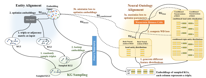
Figure 4. Architecture of NeoEA. Solid lines denote forward propagation, while dotted lines represent backward propagation. The architecture consists of three decoupled modules: (1) Entity alignment module, in which the EEA model is unaware of the existence of other modules. (2) KG sampling module, in which we sample sub-KGs to replace the whole KGs for efficiency. (3) Neural ontology alignment module, in which the discrepancy between each pair of neural axioms is estimated by Wasserstein-distance critic and optimized by gradient ascent/descent.

3.2. Conditional Neural Axiom

We can estimate the conditional distributions rather than the raw distributions to avoid the problem brought from the uniformity property. Specifically, we name conditional neural axioms to describe the entity (or triple) embedding distributions under specific semantics:

(13) $${\mathbb{A}}_{E_{h}|r_{i}} =p_{e_{h}|r_{i}}({\mathbf{e}}_{h}|{\mathbf{r}}_{i}),$$

where ${\mathbb{A}}_{E_{h}|r_{i}}$ denotes the head entity embedding distribution conditioned on the relation embedding ${\mathbf{r}}_{i}$. $p_{e_{h}|r_{i}}$ is the conditional probability distribution of the head entities given $r_{i}$. The corresponding sample set is defined as:

(14) $$E_{h}|r_{i} =\{e\,|\,\exists e^{\prime},(e,r_{i},e^{\prime})\in{\mathcal{T}}\}.$$

Following the similar rule, we can define the conditioned triple distribution ${\mathbb{A}}_{E_{h,t}|r_{i}}$ with the sample set

(15) $$E_{h,t}|r_{i}=\{(e_{h},e_{t})\,|\,(e_{h},r_{i},e_{t})\in{\mathcal{T}}\}.$$

Numerous methods have been proposed to process the neural conditioning operation, ranging from addition and concatenation (Mirza and Osindero, 2014; Wang et al., 2014; Dettmers et al., 2018), to matrix multiplication (Lin et al., 015a; Ji et al., 2015; Nguyen et al., 2016). Rather than developing new methods, we value more on its common merit: projecting the entities to a relation-specific subspace (Wang et al., 2014; Lin et al., 015a; Nguyen et al., 2016). Hence, the corresponding embedding distributions conditioned on different relations become discriminative, compared to uniformly distributed in the original embedding space.

Furthermore, conditional neural axioms capture high-level ontology knowledge:

Proposition 0 (Expressiveness).

Aligning the conditional neural axioms minimizes the embedding discrepancy of two KGs at the ontology level.

Proof.

See Appendix A for details. ∎

We take ${\mathbb{A}}_{E_{h}|r_{i}}$ as an example that summarizes the empirical “Object Property Domain” axiom of $r_{i}$ in OWL 2 EL (Baader et al., 2005). Supposed there exists such an axiom stating that the head entities of $r_{i}$ should belong to some specific class $c$ (e.g., only head entities belonging to the class ”Person” have the relation ”birthPlace”). We further suppose that there exists a classifier $f_{c}({\mathbf{e}})\in[0,1]$, such that $f_{c}({\mathbf{e}}_{j})=1$ if head entity $e_{j}$ belongs to class $c$, and $0$ otherwise. Then, with the knowledge of the given axiom, one may derive the following rule:

(16) $$\forall e\in\{e\,|\,\exists e^{\prime},(e,r_{i},e^{\prime})\in{\mathcal{T}}_{1}\cup{\mathcal{T}}_{2}\},\ f_{c}({\mathbf{e}})=1,$$

which is equivalent to:

(17) $$\mathbb{E}_{{\mathbb{A}}^{1}_{E_{h}|r_{i}}}[f_{c}({\mathbf{e}})]=\mathbb{E}_{{\mathbb{A}}^{2}_{E_{h}|r_{i}}}[f_{c}({\mathbf{e}})]=1,$$

both of which means that all head entities of $r_{i}$ in either KG should be correctly classified to $c$. Then, we have:

(18) $$\mathbb{E}_{{\mathbb{A}}_{E_{h}|r_{i}}^{1}}[f_{c}({\mathbf{e}})]-\mathbb{E}_{{\mathbb{A}}_{E_{h}|r_{i}}^{2}}[f_{c}({\mathbf{e}})]=0.$$

In fact, we do not have such knowledge about $r_{i}$ and class $c$. Instead, we can leverage a neural function $f_{c^{\prime}}({\mathbf{e}}|{\mathbf{r}}_{i})$ to estimate $f_{c}$ empirically. In this way, ${\mathbb{A}}_{E_{h}|r_{i}}^{1}$ and ${\mathbb{A}}_{E_{h}|r_{i}}^{2}$ are supposed to be aligned to minimize the loss corresponding to the above rule. Therefore, we deduce this problem back to a similar form to Equation 12, i.e.,

(19) $$\mathcal{L}_{{\mathbb{A}}_{E_{h}|r_{i}}}=\mathbb{E}_{{\mathbb{A}}_{E_{h}|r_{i}}^{1}}[f_{c^{\prime}}({\mathbf{e}}\,|\,{\mathbf{r}}_{i})]-\mathbb{E}_{{\mathbb{A}}_{E_{h}\,|\,r_{i}}^{2}}[f_{c^{\prime}}({\mathbf{e}}|{\mathbf{r}}_{i})],$$

which suggests that aligning the above conditional neural axioms can minimize the discrepancy of potential “Object Property Domain” axioms between two KGs.

Example 0 (OWL2 axiom: ObjectPropertyDomain).

As shown in Figure 3(b) and Figure 3(c), we assume that the head entities of relation “genre” are under the class “Work of Art” (although it does not exist in the dataset). It is clear that the head entity embedding distributions are only partially aligned in Figure 3(b), while those in Figure 3(c) are matched well.

In Figure 3(d), we illustrate a more complicated example. The head entities of relations “genre” and “writer” mainly belong to “Work of Art”, which show overlapped distributions (blue-orange, pink-purple) in the figure. By contrast, there exists a clear decision boundary between them and the distributions conditioned on relation “birthPlace” (red-green), as the head entities of relation “birthPlace” are under the class “Person”.

Example 0 (OWL2 axiom: SubObjectPropertyOf).

We consider two relations, “musicalArtist” and “artist” as an example, where the former is the latter’s sub-relation. In Figure 3(e), the triple distributions conditioned on “musicalArtist” (colors: pink-purple) are covered by those conditioned on “artist” (colors: orange-blue).

Algorithm 1 NeoEA

1:  Input: two KGs ${\mathcal{G}}_{1}$, ${\mathcal{G}}_{2}$, the seed alignment set ${\mathcal{S}}$, the EEA model ${\mathcal{M}}(f_{s},f_{a})$, number of steps for NeoEA $n$;

2:  Initialize all variables;

3:  repeat

4:     for $i:=1$ to $n$ do

5:        Sample sub-KGs from respective KGs ${\mathcal{G}}_{1}$, ${\mathcal{G}}_{2}$;

6:        Compute the Wasserstein-distance-based loss $\mathcal{L}_{w}$ for each pair of neural axioms;

7:        Optimize the Wasserstein distance critic $f_{w}$ by maximizing $\mathcal{L}_{w}$.

8:     end for

9:     Sample sub-KGs from respective KGs ${\mathcal{G}}_{1}$, ${\mathcal{G}}_{2}$;

10:     Compute Wasserstein-distance-based loss $\mathcal{L}_{w}$ for each pair of neural axioms;

11:     Compute the losses $\mathcal{L}_{a}$, $\mathcal{L}_{s}$ of the EEA model ${\mathcal{M}}$;

12:     Optimize the EEA model and embeddings by minimizing $\mathcal{L}_{a}$, $\mathcal{L}_{s}$, $\mathcal{L}_{w}$;

13:  until the alignment loss on the validation set converges.

3.3. Implementation

We illustrate the overall structure and training procedure in Figure 4 and Algorithm 1, respectively. The framework can be divided into three modules:

Entity Alignment. This module aims at encoding the semantics of KGs into embeddings. Almost all existing EEA models can be used here, no matter what the input data look like (e.g., triples or adjacency matrices).

KG Sampling. For each KG, we sample a sub-KG to estimate the data distributions of neural axioms. It is more efficient than separately sampling candidates for each axiom, especially when KGs get big.

Neural Ontology Alignment. As aforementioned, for each pair of embedding distributions, we align them by minimizing the empirical Wasserstein distance.

For efficiency, we share the parameters of Wasserstein distance critic only in each type of neural axiom, which reduces the number of model parameters and avoids the situation that some relations only have a small number of triples. This also allows us to perform fast mini-batch training by aligning the axioms of the same type in one operation. Given the sample KGs ${\mathcal{G}}^{\prime}_{1}=({\mathcal{E}}^{\prime}_{1},{\mathcal{R}}^{\prime}_{1},{\mathcal{T}}^{\prime}_{1})$, ${\mathcal{G}}^{\prime}_{2}=({\mathcal{E}}^{\prime}_{2},{\mathcal{R}}^{\prime}_{2},{\mathcal{T}}^{\prime}_{2})$, the corresponding batch loss is:

$$\mathcal{L}_{\mathit{sep}}= \mathcal{L}_{{\mathbb{A}}_{E^{\prime}}}$$

$$+ (\sum_{r^{\prime}\in{\mathcal{R}}^{\prime}_{1}}{\mathbb{E}_{{\mathbb{A}}_{E^{\prime}_{h}|r^{\prime}}}[f_{h|r}({\mathbf{e}}|{\mathbf{r}}^{\prime})]}$$

$$-\sum_{r^{\prime}\in{\mathcal{R}}^{\prime}_{2}}{\mathbb{E}_{{\mathbb{A}}_{E^{\prime}_{h}|r^{\prime}}}[f_{h|r}({\mathbf{e}}|{\mathbf{r}}^{\prime})]})$$

$$+ (\sum_{r^{\prime}\in{\mathcal{R}}^{\prime}_{1}}{\mathbb{E}_{{\mathbb{A}}_{E^{\prime}_{h,t}|r^{\prime}}}[f_{h,t|r}({\mathbf{e}}_{h},{\mathbf{e}}_{t}|{\mathbf{r}}^{\prime})]}$$

(20) $$-\sum_{r^{\prime}\in{\mathcal{R}}^{\prime}_{2}}{\mathbb{E}_{{\mathbb{A}}_{E^{\prime}_{h,t}|r^{\prime}}}[f_{h,t|r}({\mathbf{e}}_{h},{\mathbf{e}}_{t}|{\mathbf{r}}^{\prime})]})$$

where $\mathcal{L}_{{\mathbb{A}}_{E^{\prime}}}$ is the basic axiom loss under the sampled KGs. $f_{h|r}$ and $f_{h,t|r}$ are the critic functions of two types of neural axioms, respectively. The loss $\mathcal{L}_{\mathit{batch}}$ will approximate to that in pairwise calculation when batch-size is considerably greater than the number of relations. We take the second term in Equation (3.3) as an example. For pairwise estimation, the loss should be:

$$\sum {}_{(r_{1},r_{2})\in{\mathcal{S}}_{r}}{(\mathbb{E}_{{\mathbb{A}}_{E^{\prime}_{h}|r_{1}}}[f_{h|r}({\mathbf{e}}|{\mathbf{r}}_{1})]-\mathbb{E}_{{\mathbb{A}}_{E^{\prime}_{h}|r_{2}}}[f_{h|r}({\mathbf{e}}|{\mathbf{r}}_{2})])}$$

$$= \sum_{(r_{1},r_{2})\in{\mathcal{S}}_{r}}{\mathbb{E}_{{\mathbb{A}}_{E^{\prime}_{h}|r_{1}}}[f_{h|r}({\mathbf{e}}|{\mathbf{r}}_{1})]}$$

(21) $$- \sum_{(r_{1},r_{2})\in{\mathcal{S}}_{r}}{\mathbb{E}_{{\mathbb{A}}_{E^{\prime}_{h}|r_{2}}}[f_{h|r}({\mathbf{e}}|{\mathbf{r}}_{2})]},$$

where ${\mathcal{S}}_{r}\subset{\mathcal{R}}_{1}\times{\mathcal{R}}_{2}$ denotes the set of all aligned relation pairs. The above equation suggests that the pairwise loss is based on the respective relation sets of two KGs, not constrained by each pair of aligned relations. Generally, the number of relations is much smaller than the number of sampled triples in one batch, which means that ${\mathcal{R}}^{\prime}_{1},{\mathcal{R}}^{\prime}_{2}$ in Equation (3.3) can cover a large proportion of elements in the full relation sets ${\mathcal{R}}_{1}$, ${\mathcal{R}}_{2}$. Therefore, we used $\mathcal{L}_{\mathit{batch}}$ to approximate the pairwise loss in the implementation.

4. Experiments

Table 1. Results on V1 datasets (5-fold cross-validation).

Models	EN-FR			EN-DE			D-W			D-Y
	H@1	H@5	MRR	H@1	H@5	MRR	H@1	H@5	MRR	H@1	H@5	MRR
RSN (Guo et al., 2019)	.393	.595	.487	.587	.752	.662	.441	.615	.521	.514	.655	.580
RSN + NeoEA	.399	.597	.490	.600	.759	.673	.450	.624	.530	.522	.663	.588
SEA (Pei et al., 2019b)	.280	.530	.397	.530	.718	.617	.360	.572	.458	.500	.706	.591
SEA + NeoEA	.320	.584	.443	.586	.766	.668	.389	.608	.490	.549	.752	.638
BootEA (Sun et al., 2018)	.507	.718	.603	.675	.820	.740	.572	.744	.649	.739	.849	.788
BootEA + NeoEA	.521	.733	.617	.676	.820	.740	.579	.753	.658	.756	.859	.797
RDGCN (Wu et al., 2019)	.755	.854	.800	.830	.895	.859	.515	.669	.584	.931	.969	.949
RDGCN + NeoEA	.775	.868	.817	.846	.908	.874	.527	.671	.592	.941	.972	.955

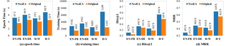
Figure 5. Results on OpenEA 100K datasets.

In this section, we empirically verify the effectiveness of NeoEA by a series of experiments with state-of-the-art methods as baselines. The source code was uploaded .

4.1. Settings

We selected four best-performing and representative models as our baselines:

• RSN (Guo et al., 2019), an RNN-based EEA model with only structure data as input.

• SEA (Pei et al., 2019b), a TransE-based model with both structure and attribute data as input.

• BootEA (Sun et al., 2018), a TransE-based EEA model with only structure data as input.

• RDGCN (Wu et al., 2019), a GCN-based model with both structure and attribute data as input.

The whole framework is based on OpenEA (Sun et al., 2020b). We modified only the initialization of the original project. In this sense, the EEA models were unaware of the existence of neural ontologies. Furthermore, we kept the optimal hyper-parameter settings in OpenEA to ensure a fair comparison.

The data distributions of some previous benchmarks such as JAPE (Sun et al., 2017) and BootEA (Sun et al., 2018) are different from those of real-world KGs, which means that conducting experiments on those benchmarks cannot reflect the realistic performance of an EEA model (Guo et al., 2019; Sun et al., 2020b). Therefore, we consider the latest benchmark provided by OpenEA (Sun et al., 2020b), which consists of four sub-datasets with two density settings. Specifically, “D-W”, “D-Y” denote “DBpedia (Auer et al., 2007)-WikiData (Vrandečić and Krötzsch, 2014)”, “DBpedia-YAGO (Fabian et al., 2007)”, respectively. “EN-DE” and “EN-FR’ denote two cross-lingual datasets, both of which are sampled from DBpedia. Each sampled KG has around 15,000 entities. The entity degree distributions in “V1” datasets are similar to those in the original KGs, while the average degree in “V2” datasets are doubled. For detailed statistics of the datasets, please refer to (Sun et al., 2020b).

4.2. Empirical Comparisons

Table 2. Results of ablation study based on the best-performing model RDGCN, on V1 datasets.

Models	EN-FR			EN-DE			D-W			D-Y
	H@1	H@5	MRR	H@1	H@5	MRR	H@1	H@5	MRR	H@1	H@5	MRR
Full	.775	.868	.817	.846	.908	.874	.527	.671	.592	.941	.972	.955
Partial	.771	.863	.813	.840	.900	.871	.523	.669	.590	.936	.971	.952
Basic	.755	.853	.799	.827	.895	.858	.512	.656	.578	.931	.969	.948
Original	.755	.854	.800	.830	.895	.859	.515	.669	.584	.931	.969	.949

The main results on V1 datasets are shown in Table 1. Although the performance of four baseline models varied from different datasets, all of them gained improvement with NeoEA. This demonstrates that aligning the neural ontology is beneficial for all four kinds of EEA models.

On the other hand, we find that the performance improvement on SEA and RDGCN was more significant than that on BootEA and RSN, as the latter two are not typical EEA models. BootEA has a sophisticated bootstrapping procedure, which may be challenging to be injected with NeoEA. RSN tries to capture long-term dependencies. The complicated objective may conflict with NeoEA more or less. Even though we still observe relatively significant improvement on some datasets (e.g., EN-DE and D-Y). Therefore, we believe their performance can be refined through a joint hyper-parameter turning with NeoEA, which we leave to future work.

The results on V2 datasets (i.e., the denser and simpler ones) are presented in Appendix B. Briefly, the improvement is relatively smaller than that on V1 datasets because the average entity degree is doubled. However, NeoEA still outperformed all the baselines. Those results empirically proved its effectiveness.

4.3. The Scalability and Efficiency of NeoEA

We also conducted experiment on the OpenEA 100K datasets to evaluate performance of NeoEA on larger KGs. We used a single TITAN RTX for training, and SEA (the fastest model) as the basic EEA model. In theory, NeoEA does not have multiple GCN/GAT layers nor the pair-wise similarity estimation on whole graphs. The embedding distributions are also obtained from the sampled KG. Therefore, NeoEA is applicable to large-scale datasets.

The results are shown in Figure 5, from which we can find that the time for training one epoch (Figure 5a) was not evidently increased, especially considering the cost of switching the optimizers. On the other hand, the overall training time was nearly doubled (Figure 5b), caused by the adversarial training procedure. Even thought the loss converged more slowly in NeoEA, we should notice that the overall training time was much less than that of complicated EEA models, e.g., BootEA (35,000+ seconds). In Figures 5c and 5d, we can find that the improvement for Hits@1 and MRR was significant, especially on the D-Y dataset that took longest time in training.

4.4. The Necessity of Conditioned Neural Axioms

We designed an experiment to verify some claims in Section 3. We choose the best-performing model RDGCN as our baseline. As shown in Table 2, “Full” denotes NeoEA with the full set of neural axioms. “Partial” denotes NeoEA without the conditional triple axioms. We further removed the conditional entity axioms from “Partial” to construct “Basic”, and the last one, “Original”, denotes the original EEA model.

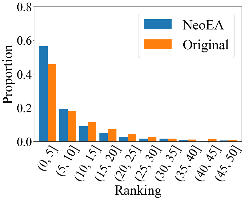
(a) rankings of long-tail entities

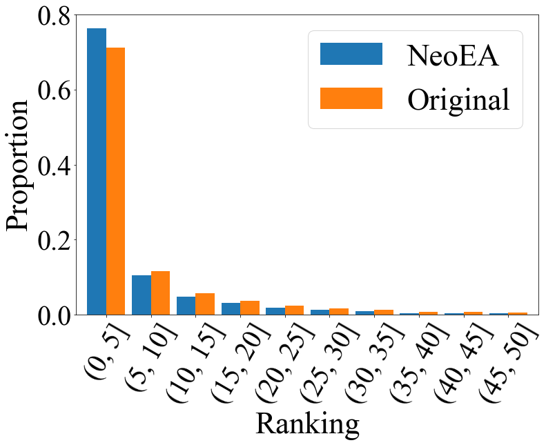
(b) rankings of popular entities

Figure 6. Normalized histograms of alignment rankings on EN-FR, V1 dataset.

It is clear that aligning the basic axiom was less effective or even harmful to the model. This result empirically demonstrates our assumption that the uniformity property of the learned entity embeddings will make the embedding distribution alignment meaningless. On the other hand, aligning only a part of conditional axioms ${\mathbb{A}}_{E_{h}|r_{i}},{\mathbb{A}}_{E_{t}|r_{i}}$ that describe entity embedding distributions conditioned on relation embeddings was significantly helpful for the model. Also, the additional improvement was observed with the full conditional axioms.

Note that the improvement from “Partial” to “Full” was not as significant as that from ”Basic” to “Partial”. This is because the triple neural axioms mainly describe the relationships between different relations (see Appendix A). Due to the sampling strategy of the datasets, the number of relations is relatively small. Few correlated relation pairs exist in the datasets, resulting in limited improvement.

4.5. Further Analysis of the Bound

We have shown that the embedding discrepancy between each underlying aligned pair is bounded by $\epsilon$ associated with $\lambda$ in Section 2. In this section, we provide empirical statistics to verify this point. To this end, we manually split the entities into two groups: (1) long-tail entities, which have at most two neighbors that do not belong to known aligned pairs; (2) popular entities, the remaining.

We draw the histograms of alignment rankings w.r.t. respective groups based on the EEA model SEA. From Figure 6, we can find that the proportion of the inexact alignments (i.e., ranking $>5$) for long-tail entities is evidently larger than that of popular entities, especially for the bins $(5,20]$. This observation verified that the long-tail entities are less constrained compared to those popular entities in EEA problem.

Furthermore, with NeoEA, the rankings of those long-tail entities were improved more significantly than those of popular entities, which demonstrates that NeoEA indeed tightened the representation discrepancy of those less restrained entities.

We report the average ranking improvement on four V1 datasets in Figure 7, which shows consistent results. It is worth noting that the ranking improvement for long-tail entities is more than twice as larger as that for popular entities, except the D-W dataset.

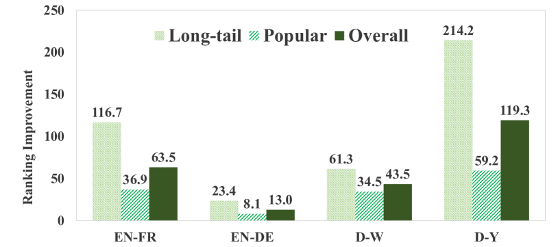
Figure 7. The average ranking improvement on different groups of entities.

5. Conclusion and Future Work

In this paper, we proposed a new approach to learn KG embeddings for entity alignment. We proved its expressiveness theoretically and demonstrated its efficiency by conducting extensive experiments on the latest benchmarks. We observed that four state-of-the-art EEA methods gained evident benefits with NeoEA. Moreover, we showed that the proposed conditional neural axioms are the key to improve the performance of current EEA methods. For future work, we plan to study how to extend NeoEA with realistic ontology knowledge for further improvement.

Appendix A Proof for Proposition 2

Proposition 3 (Expressiveness).

Aligning the conditional neural axioms minimizes the embedding discrepancy of two KGs at the ontology level.

Proof.

We split the proofs according to the types of axioms in OWL2 EL (Baader et al., 2005):

ObjectPropertyDomain, ObjectPropertyRange. The proof for ObjectPropertyDomain has been presented in Section 3, and that for ObjectPropertyRange is similar.

ReflexiveObjectProperty, IrreflexiveObjectProperty. If we say that a relation $r_{i}$ is reflexive, it must satisfy

(22) $$\forall(e,r_{i},e^{\prime})\in{\mathcal{T}},\ (e,r_{i},e)\in{\mathcal{T}},$$

which means each head entities of $r_{i}$ must be connected by $r_{i}$ to itself. The above rule suggests that we can align the underlying reflexive knowledge by minimizing the discrepancy between triple distributions conditioned on relation $r_{i}$, i.e., aligning ${\mathbb{A}}_{E_{(h,t)}|r_{i}}^{1}$ with ${\mathbb{A}}_{E_{(h,t)}|r_{i}}^{2}$. The similar to IrreflexiveObjectProperty axiom.

FunctionalObjectProperty, InverseFunctionalObjectProperty. We first introduce FunctionalObjectProperty axiom. It compels each head entity $e$ connected by relation $r_{i}$ to have exactly one tail entity, implying the following rule:

(23) $$\forall(e,r_{i},e^{\prime})\in{\mathcal{T}},\forall e^{\prime\prime}\in{\mathcal{E}},\ (e,r_{i},e^{\prime\prime})\notin{\mathcal{T}}.$$

The above rule is also related to the triple distribution conditioned on $r_{i}$. The similar to the InverseFunctionalObjectProperty axiom.

SymmetricObjectProperty, AsymmetricObjectProperty. The first axiom can state a relation $r_{i}$ is symmetric, that is,

(24) $$\forall(e,r_{i},e^{\prime})\in{\mathcal{T}},\ (e^{\prime},r_{i},e)\in{\mathcal{T}}.$$

It is also related to the triple distributions referred to $r_{i}$, implying that aligning ${\mathbb{A}}_{E_{(h,t)}|r_{i}}^{1}$ with ${\mathbb{A}}_{E_{(h,t)}|r_{i}}^{2}$ is sufficient to minimize the difference. The similar to the AsymmetricObjectProperty axiom.

SubObjectPropertyOf, EquivalentObjectProperties, DisjointObjectProperties and InverseObjectProperties. We show that these axioms also define rules related to triple distributions conditioned on relations. We start from SubObjectPropertyOf, which can state that relation $r_{i}$ is a sub-property of relation $r_{j}$ (e.g., “hasDog” is one of the sub-properties of “hasPet”). We formulate it as

(25) $$\forall(e,r_{i},e^{\prime})\in{\mathcal{T}},\ (e^{\prime},r_{j},e)\in{\mathcal{T}}.$$

To align the potential SubObjectPropertyOf axioms between two KGs, we can respectively align $({\mathbb{A}}_{E_{(h,t)}|r_{i}}^{1},{\mathbb{A}}_{E_{(h,t)}|r_{i}}^{2})$ and $({\mathbb{A}}_{E_{(h,t)}|r_{j}}^{1},{\mathbb{A}}_{E_{(h,t)}|r_{j}}^{2})$, such that the joint one $({\mathbb{A}}_{E_{(h,t)}|r_{i},r_{j}}^{1},{\mathbb{A}}_{E_{(h,t)}|r_{i},r_{j}}^{2})$ will also be aligned.

Similarly, if $r_{i}$ and $r_{j}$ are equivalent, we can interpret the axiom as

(26)

If they are disjoint, the corresponding rule will be

(27) $$\forall(e,r_{i},e^{\prime})\in{\mathcal{T}},\ (e,r_{j},e^{\prime})\notin{\mathcal{T}}.$$

If they are inverse to each other, the rule is

(28) $$\forall(e,r_{i},e^{\prime})\in{\mathcal{T}},\ (e^{\prime},r_{j},e)\in{\mathcal{T}}.$$

TransitiveObjectProperty. We show that this axiom is also related to triple distributions conditioned on $r_{i}$. Supposed that a relation $r_{i}$ is transitive, then one can derive the following rule:

(29) $$\forall(e,r_{i},e^{\prime})\in{\mathcal{T}}\&(e^{\prime},r_{i},e^{\prime\prime})\in{\mathcal{T}},\ (e,r_{i},e^{\prime\prime})\in{\mathcal{T}},$$

which means we can align the potential TransitiveObjectProperty axioms via minimizing the distribution discrepancy between ${\mathbb{A}}_{E_{(h,t)}|r_{i}}^{1}$ and ${\mathbb{A}}_{E_{(h,t)}|r_{i}}^{2}$. ∎

Appendix B Results on V2 Datasets

The results on V2 datasets are shown in Table 3. Although entities have doubled number of neighbors in V2 datasets, all baseline models still gained significant improvement with NeoEA.

Table 3. Results on V2 datasets (5-fold cross-validation).

Models	EN-FR			EN-DE			D-W			D-Y
	H@1	H@5	MRR	H@1	H@5	MRR	H@1	H@5	MRR	H@1	H@5	MRR
RSN (Guo et al., 2019)	.579	.759	.662	.791	.890	.837	.723	.854	.782	.933	.974	.951
RSN + NeoEA	.583	.760	.666	.794	.892	.839	.729	.858	.787	.935	.976	.953
SEA (Pei et al., 2019b)	.360	.651	.494	.606	.779	.687	.567	.770	.660	.899	.950	.923
SEA + NeoEA	.375	.666	.508	.637	.800	.712	.588	.784	.677	.917	.959	.936
BootEA (Sun et al., 2018)	.660	.850	.745	.833	.912	.869	.821	.926	.867	.958	.984	.969
BootEA + NeoEA	.665	.853	.749	.834	.916	.870	.822	.926	.869	.958	.984	.969
RDGCN (Wu et al., 2019)	.847	.919	.880	.833	.891	.860	.623	.757	.684	.936	.966	.950
RDGCN + NeoEA	.864	.933	.896	.849	.902	.874	.632	.760	.690	.940	.970	.953

References

- (1)
- Arjovsky et al. (2017) Martín Arjovsky, Soumith Chintala, and Léon Bottou. 2017. Wasserstein GAN. CoRR (2017). arXiv:1701.07875
- Auer et al. (2007) Sören Auer, Christian Bizer, Georgi Kobilarov, Jens Lehmann, Richard Cyganiak, and Zachary G. Ives. 2007. DBpedia: A nucleus for a web of open data. In ISWC. 722–735.
- Baader et al. (2005) Franz Baader, Sebastian Brandt, and Carsten Lutz. 2005. Pushing the EL Envelope. In IJCAI. 364–369.
- Ben-David et al. (2010) Shai Ben-David, John Blitzer, Koby Crammer, Alex Kulesza, Fernando Pereira, and Jennifer Wortman Vaughan. 2010. A theory of learning from different domains. Mach. Learn. 79 (2010), 151–175.
- Bordes et al. (2013) Antoine Bordes, Nicolas Usunier, Alberto Garcia-Durán, Jason Weston, and Oksana Yakhnenko. 2013. Translating embeddings for modeling multi-relational data. In NIPS. 2787–2795.
- Chen et al. (2021) Jiaoyan Chen, Pan Hu, Ernesto Jiménez-Ruiz, Ole Magnus Holter, Denvar Antonyrajah, and Ian Horrocks. 2021. OWL2Vec*: embedding of OWL ontologies. Mach. Learn. 110, 7 (2021), 1813–1845.
- Chen et al. (2017) Muhao Chen, Yingtao Tian, Mohan Yang, and Carlo Zaniolo. 2017. Multilingual knowledge graph embeddings for cross-lingual knowledge alignment. In IJCAI. 1511–1517.
- Courty et al. (2017) Nicolas Courty, Rémi Flamary, Amaury Habrard, and Alain Rakotomamonjy. 2017. Joint distribution optimal transportation for domain adaptation. In NeurIPS. 3730–3739.
- Dettmers et al. (2018) Tim Dettmers, Pasquale Minervini, Pontus Stenetorp, and Sebastian Riedel. 2018. Convolutional 2D knowledge graph embeddings. In AAAI. 1811–1818.
- El-Roby and Aboulnaga (2015) Ahmed El-Roby and Ashraf Aboulnaga. 2015. ALEX: Automatic link exploration in linked data. In SIGMOD. Melbourne, Australia, 1839–1853.
- Fabian et al. (2007) MS Fabian, Kasneci Gjergji, WEIKUM Gerhard, et al. 2007. Yago: A core of semantic knowledge unifying wordnet and wikipedia. In WWW. 697–706.
- Fey et al. (2020) Matthias Fey, Jan Eric Lenssen, Christopher Morris, Jonathan Masci, and Nils M. Kriege. 2020. Deep Graph Matching Consensus. In ICLR. https://openreview.net/forum?id=HyeJf1HKvS
- Ganin and Lempitsky (2015) Yaroslav Ganin and Victor S. Lempitsky. 2015. Unsupervised Domain Adaptation by Backpropagation. In ICML. 1180–1189.
- Goodfellow et al. (2014) Ian J. Goodfellow, Jean Pouget-Abadie, Mehdi Mirza, Bing Xu, David Warde-Farley, Sherjil Ozair, Aaron Courville, and Yoshua Bengio. 2014. Generative Adversarial Networks. arXiv:1406.2661
- Grau et al. (2008) Bernardo Cuenca Grau, Ian Horrocks, Boris Motik, Bijan Parsia, Peter F. Patel-Schneider, and Ulrike Sattler. 2008. OWL 2: The next step for OWL. J. Web Semant. 6, 4 (2008), 309–322.
- Guo et al. (2019) Lingbing Guo, Zequn Sun, and Wei Hu. 2019. Learning to Exploit Long-term Relational Dependencies in Knowledge Graphs. In ICML. 2505–2514.
- Horrocks et al. (2006) Ian Horrocks, Oliver Kutz, and Ulrike Sattler. 2006. The Even More Irresistible SROIQ. In Proceedings, Tenth International Conference on Principles of Knowledge Representation and Reasoning, Lake District of the United Kingdom, June 2-5, 2006, Patrick Doherty, John Mylopoulos, and Christopher A. Welty (Eds.). AAAI Press, 57–67. http://www.aaai.org/Library/KR/2006/kr06-009.php
- Ji et al. (2015) Guoliang Ji, Shizhu He, Liheng Xu, Kang Liu, and Jun Zhao. 2015. Knowledge graph embedding via dynamic mapping matrix. In ACL. 687–696.
- Kazemi and Poole (2018) Seyed Mehran Kazemi and David Poole. 2018. SimplE embedding for link prediction in knowledge graphs. In NeurlIPS. Montréal, Canada, 4289–4300.
- Lacoste-Julien et al. (2013) Simon Lacoste-Julien, Konstantina Palla, Alex Davies, Gjergji Kasneci, Thore Graepel, and Zoubin Ghahramani. 2013. SiGMa: Simple greedy matching for aligning large knowledge bases. In KDD. Chicago, IL, USA, 572–580.
- Lin et al. (015a) Yankai Lin, Zhiyuan Liu, Maosong Sun, Yang Liu, and Xuan Zhu. 2015a. Learning entity and relation embeddings for knowledge graph completion. In AAAI. 2181–2187.
- Mirza and Osindero (2014) Mehdi Mirza and Simon Osindero. 2014. Conditional Generative Adversarial Nets. CoRR (2014). arXiv:1411.1784
- Nguyen et al. (2016) Dat Quoc Nguyen, Kairit Sirts, Lizhen Qu, and Mark Johnson. 2016. STransE: A novel embedding model of entities and relationships in knowledge bases. In NAACL. San Diego, USA, 460–466.
- Pei et al. (2019b) Shichao Pei, Lu Yu, Robert Hoehndorf, and Xiangliang Zhang. 2019b. Semi-supervised entity alignment via knowledge graph embedding with awareness of degree difference. In WWW. 3130–3136.
- Pei et al. (2019a) Shichao Pei, Lu Yu, and Xiangliang Zhang. 2019a. Improving Cross-lingual Entity Alignment via Optimal Transport. In IJCAI. 3231–3237.
- Shen et al. (2018) Jian Shen, Yanru Qu, Weinan Zhang, and Yong Yu. 2018. Wasserstein Distance Guided Representation Learning for Domain Adaptation. In AAAI. 4058–4065.
- Suchanek et al. (2012) Fabian M. Suchanek, Serge Abiteboul, and Pierre Senellart. 2012. PARIS: Probabilistic alignment of relations, instances, and schema. PVLDB 5 (2012), 157–168.
- Sun et al. (2017) Zequn Sun, Wei Hu, and Chengkai Li. 2017. Cross-lingual entity alignment via joint attribute-preserving embedding. In ISWC. 628–644.
- Sun et al. (2018) Zequn Sun, Wei Hu, Qingheng Zhang, and Yuzhong Qu. 2018. Bootstrapping entity alignment with knowledge graph embedding. In IJCAI. 4396–4402.
- Sun et al. (2020a) Zequn Sun, Chengming Wang, Wei Hu, Muhao Chen, Jian Dai, Wei Zhang, and Yuzhong Qu. 2020a. Knowledge Graph Alignment Network with Gated Multi-hop Neighborhood Aggregation. In AAAI. 222–229.
- Sun et al. (2020b) Zequn Sun, Qingheng Zhang, Wei Hu, Chengming Wang, Muhao Chen, Farahnaz Akrami, and Chengkai Li. 2020b. A Benchmarking Study of Embedding-based Entity Alignment for Knowledge Graphs. CoRR abs/2003.07743 (2020).
- Trouillon et al. (2016) Théo Trouillon, Johannes Welbl, Sebastian Riedel, Éric Gaussier, and Guillaume Bouchard. 2016. Complex embeddings for simple link prediction. In ICML. 2071–2080.
- Vrandečić and Krötzsch (2014) Denny Vrandečić and Markus Krötzsch. 2014. Wikidata: a free collaborative knowledgebase. Commun. ACM 57 (2014), 78–85.
- Wang and Isola (2020) Tongzhou Wang and Phillip Isola. 2020. Understanding Contrastive Representation Learning through Alignment and Uniformity on the Hypersphere. In ICML. 9929–9939.
- Wang et al. (2018a) Yanjie Wang, Rainer Gemulla, and Hui Li. 2018a. On Multi-Relational Link Prediction With Bilinear Models. In AAAI. 4227–4234.
- Wang et al. (2018b) Zhichun Wang, Qingsong Lv, Xiaohan Lan, and Yu Zhang. 2018b. Cross-lingual knowledge graph alignment via graph convolutional networks. In EMNLP. 349–357.
- Wang et al. (2014) Zhen Wang, Jianwen Zhang, Jianlin Feng, and Zheng Chen. 2014. Knowledge graph embedding by translating on hyperplanes. In AAAI. 1112–1119.
- Wu et al. (2019) Yuting Wu, Xiao Liu, Yansong Feng, Zheng Wang, Rui Yan, and Dongyan Zhao. 2019. Relation-Aware Entity Alignment for Heterogeneous Knowledge Graphs. In IJCAI. 5278–5284.
- Yang et al. (2015) Bishan Yang, Wen-tau Yih, Xiaodong He, Jianfeng Gao, and Li Deng. 2015. Embedding entities and relations for learning and inference in knowledge bases. In ICLR. http://arxiv.org/abs/1412.6575
- Ye et al. (2019) Rui Ye, Xin Li, Yujie Fang, Hongyu Zang, and Mingzhong Wang. 2019. A Vectorized Relational Graph Convolutional Network for Multi-Relational Network Alignment. In IJCAI. 4135–4141.
- Zhu et al. (2017) Hao Zhu, Ruobing Xie, Zhiyuan Liu, and Maosong Sun. 2017. Iterative entity alignment via joint knowledge embeddings. In IJCAI. 4258–4264.