Utilizing Redundancy in Cost Functions
for Resilience in Distributed Optimization and Learning

Abstract

This paper considers the problem of resilient distributed optimization and stochastic machine learning in a server-based architecture. The system comprises a server and multiple agents, where each agent has a local cost function. The agents collaborate with the server to find a minimum of their aggregate cost functions. We consider the case when some of the agents may be asynchronous and/or Byzantine faulty. In this case, the classical algorithm of distributed gradient descent (DGD) is rendered ineffective. Our goal is to design techniques improving the efficacy of DGD with asynchrony and Byzantine failures. To do so, we start by proposing a way to model the agents’ cost functions by the generic notion of $(f,\,r;\epsilon)$-redundancy where $f$ and $r$ are the parameters of Byzantine failures and asynchrony, respectively, and $\epsilon$ characterizes the closeness between agents’ cost functions. This allows us to quantify the level of redundancy present amongst the agents’ cost functions, for any given distributed optimization problem. We demonstrate, both theoretically and empirically, the merits of our proposed redundancy model in improving the robustness of DGD against asynchronous and Byzantine agents, and their extensions to distributed stochastic gradient descent (D-SGD) for robust distributed machine learning with asynchronous and Byzantine agents.

1 Introduction

With the rapid growth in the computational power of modern computer systems and the scale of optimization tasks, e.g., learning of deep neural networks [39], the problem of distributed optimization over a multi-agent system has gained significant attention in recent years. In the setting of multi-agent system, each agent has a local cost function. The goal is to design an algorithm that allows the agents to collectively minimize the aggregated cost functions of all agents [9]. Formally, we suppose that there are $n$ agents in the system where each agent $i$ has a cost function $Q_{i}:\mathbb{R}^{d}\to\mathbb{R}$. A distributed optimization algorithm enables the agents to compute a global minimum $x^{*}$ such that

$$x^{*}\in\arg\min_{x\in\mathbb{R}^{d}}\sum_{i=1}^{n}Q_{i}(x).$$ (1)

For example, amongst a group of $n$ people, the function $Q_{i}(x)$ may represent the cost of each person $i$ to travel to some location $x$, and thus, $x^{*}$ represents a location that minimizes the aggregate (or average) travel cost for all the $n$ people. Besides the obvious application to distributed machine learning [9], the above multi-agent optimization problem finds many other applications, such as distributed sensing [41], and swarm robotics [42].

Distributed optimization systems, however, encounter some issues in practice; such as presence of faulty agents that send wrong information and stragglers that operate slowly. Prior works have shown that even a single faulty agent can compromise the entire distributed optimization process [11, 47]. Stragglers, on the other hand, can lead to computational inefficiencies wasting resources [21, 30, 4]. These issues require further attention and have sparked a plethora of research [10, 5, 35, 48, 20, 23, 38].

Resilient distributed optimization refers to the problem of distributed optimization when there are faulty agents and/or stragglers in the system. Specifically, there are 4 types of problems listed below and summarized in Table 1.

Problem A

Distributed optimization in a synchronous system with no faulty agents

Problem B

Distributed optimization in a synchronous system with faulty agents

Problem C

Asynchronous distributed optimization with no faulty agents

Problem D

Asynchronous distributed optimization with faulty agents

Problem A has been well studied in the past, and can be solved using several existing distributed optimization algorithms [9, 37, 46, 49]. Problems B, C and D on the other hand require use of techniques to irregularities due to faulty agents and/or asynchrony. Note that for faulty agents, we consider a Byzantine fault model [28], where no constraints are imposed on the behavior of the faulty agents.

Table 1: Problems in Resilient Distributed Optimization.

	No faulty agents	Faulty agents
Synchronous	A	B
Asynchronous	C	D

To formally study each of the above problems, we define the objective of resilient distributed optimization by the notion of $(f,r;\epsilon)$-resilience stated below. Recall that the Euclidean distance between a point $x$ and a set $Y$ in $\mathbb{R}^{d}$, denoted by $\mathrm{dist}\left(x,\,Y\right)$, is defined to be

$$\mathrm{dist}\left(x,\,Y\right)=\inf_{y\in Y}\mathrm{dist}\left(x,\,y\right)=\inf_{y\in Y}\left\lVert x-y\right\rVert,$$

where $\left\lVert\cdot\right\rVert$ represents the Euclidean norm.

Definition 1 ($(f,r;\epsilon)$-resilience).

For $\epsilon\geq 0$, a distributed optimization algorithm is said to be $(f,r;\epsilon)$-resilient if its output $\widehat{x}$ satisfies

$$\mathrm{dist}\left(\widehat{x},\,\arg\min_{x\in\mathbb{R}^{d}}\sum_{i\in\mathcal{H}}Q_{i}(x)\right)\leq\epsilon$$

for each set $\mathcal{H}$ of $n-f$ non-faulty agents, despite the presence of up to $f$ faulty agents and up to $r$ stragglers.

In this paper, we show how redundancy in agents’ cost functions can be utilized to obtain $(f,r;\epsilon)$-resilience. Specifically, we consider a redundancy property of the agents’ cost functions, named $(f,r;\epsilon)$-redundancy, as defined below. Recall that the Hausdorff distance between two sets $X$ and $Y$ in $\mathbb{R}^{d}$, denoted by $\mathrm{dist}\left(X,\,Y\right)$, is defined to be

$$\mathrm{dist}\left(X,\,Y\right)\triangleq\max\left\{\sup_{x\in X}\mathrm{dist}\left(x,\,Y\right),\sup_{y\in Y}\mathrm{dist}\left(y,\,X\right)\right\}.$$

Definition 2 ($(f,r;\epsilon)$-redundancy).

For $\epsilon\geq 0$, the agents’ cost functions are said to satisfy the $(f,r;\epsilon)$-redundancy property if and only if the distance between the minimum point sets of the aggregated cost functions of any pair of subsets of agents $S,\widehat{S}\subsetneq\{1,...,n\}$, where $\left\lvert S\right\rvert=n-f$, $\left\lvert\widehat{S}\right\rvert\geq n-r-2f$ and $\widehat{S}\subsetneq S$, is bounded by $\epsilon$, i.e.,

$$\mathrm{dist}\left(\arg\min_{x}\sum_{i\in S}Q_{i}(x),\,\arg\min_{x}\sum_{i\in\widehat{S}}Q_{i}(x)\right)\leq\epsilon.$$

It should be noted that for any distributed optimization problem, for any $r<n$ and $f<(n-r)/2$, there exists $\epsilon\geq 0$ such that the agents’ cost functions satisfy the $(f,r;\epsilon)$-redundancy property. Intuitively, the above redundancy property indicates the loss in accuracy due to losing some of agents in the system during the optimization process. For a fixed $f$ and $r$, smaller $\epsilon$ indicates more redundancy. On the other hand, for a fixed $\epsilon$, smaller $f$ or $r$ indicates less redundancy.

Next, we consider distributed gradient descent (DGD) based algorithms where a server maintains an estimate for the optimum. In each iteration of the algorithm, the server sends this estimate to the agents, and the agents send the gradients of their local cost functions at that estimate to the server. The server uses these gradients to update the estimate. Specifically, Algorithm 1 is a framework for several instances of the distributed optimization algorithms presented later in this paper. The main difference between these different algorithms is in the manner in which they perform the iterative update (2) at the server – different gradient aggregators are used when solving different instances of the distributed optimization problems. A gradient aggregator $\mathsf{GradAgg}(\cdot;n,f,r):\mathbb{R}^{d\times(n-r)}\rightarrow\mathbb{R}^{d}$ is a function that takes $n-r$ vectors in $\mathbb{R}^{d}$ (gradients) and outputs a vector in $\mathbb{R}^{d}$ for the update, with the knowledge that there are up to $f$ Byzantine faulty agents and up to $r$ stragglers out of the $n$ agents in the system. The compact set $\mathcal{W}$ contains the true solution to the problem. We will explain the details when introducing our convergence analyses.

Input: $n$, $f$, $r$, $\epsilon$. A convex compact set $\mathcal{W}$. Each agent $i$ has its cost function $Q_{i}(x)$.

The initial estimate of the optimum, $x^{0}$, is chosen by the server in $\mathcal{W}$. The new estimate $x^{t+1}$ is computed in iteration $t\geq 0$ as follows:

Step 1:

The server requests each agent for the gradient of its local cost function at the current estimate $x^{t}$. Each agent $j$ is expected to send to the server the gradient (or stochastic gradient) $g_{j}^{t}$ with timestamp $t$.

Step 2:

The server waits until it receives $n-r$ gradients with the timestamp of $t$. Suppose $S^{t}\subseteq\{1,...,n\}$ is the set of agents whose gradients are received by the server at step $t$ where $\left\lvert S^{t}\right\rvert=n-r$. The server updates its estimate to

$$x^{t+1}=\left[x^{t}-\eta_{t}\,\mathsf{GradAgg}\left(g_{j}^{t}|\,j\in S^{t};n,f,r\right)\right]_{\mathcal{W}}$$ (2)

where $\eta_{t}\geq 0$ is the step-size for each iteration $t$, and $[\,\cdot\,]_{\mathcal{W}}$ denotes a projection onto $\mathcal{W}$.

Algorithm 1 Resilient distributed gradient-descent under $(f,r;\epsilon)$-redundancy

1.1 Distributed machine learning

Distributed machine learning is a special case of distributed optimization. We consider a machine learning model $\Pi$ characterized by a real-valued parameter vector $x\in\mathbb{R}^{d}$. Each agent $i$ has a data generation distribution $\mathcal{D}_{i}$ over $\mathbb{R}^{m}$. Each data point $z\in\mathbb{R}^{m}$ is a real-valued vector that incurs a cost defined by a loss function $\ell:(x;z)\mapsto\mathbb{R}$. The expected loss function for each agent $j$ can be defined as

$$Q_{i}(x)=\mathbb{E}_{z\sim\mathcal{D}_{i}}\ell(x;z),~{}\textrm{ for all }x\in\mathbb{R}^{d}.$$ (3)

The goal of training a machine learning model $\Pi$ is to minimize the aggregate cost over all the agents, which is of the same form as (1).

Stochastic gradient descent is a more efficient method than descent-based method using full gradients for machine learning tasks [6, 7, 8], and therefore more commonly used. Resilient distributed stochastic learning problem also has 4 types, corresponding to the four problems in Table 1, summarized below. To solve these problems, we use stochastic optimization algorithms, with each agent’s expected cost function defined in (3).

Problem AS

Synchronous system, no faulty agents

Problem BS

Synchronous system with faulty agents

Problem CS

Asynchronous system, no faulty agents

Problem DS

Asynchronous system with faulty agents

We discuss the stochastic version of Algorithm 1 with D-SGD in detail in Section 4.

1.2 Open problems in the problem space

We briefly discuss the current status of problems listed in Table 1 and their distributed learning counterparts.

Problems A, B and AS have been solved previously. In particular, as stated above, Problem A can be solved by DGD with standard convexity assumptions on the cost functions without redundancy. It was previously shown that $(f,0;\epsilon)$-redundancy is necessary and sufficient to solve Problem B [17, 35]. For the stochastic case, Problem AS has been solved using D-SGD with convexity assumptions and without redundancy [33].

In this paper, we show how to utilize redundancy to solve Problems C, D, BS, CS, and DS. The rest of the paper is organized as follows: We discuss other related work in Section 2. We then provide analyses on different versions of Algorithm 1, namely asymptotic convergence for optimization problems in Section 3, and convergence rate results for learning problems in Section 4. Empirical results are provided in Section 5. Finally, we summarize the paper and discuss limitations in our results in Section 6.

Proofs for all theorems and the code for experiments can be found in the supplementary materials.

2 Related work

Byzantine fault-tolerant optimization Byzantine agents make the goal of distributed optimization (1) generally impossible. However, prior work has shown that the goal of minimizing the aggregate cost function of only the non-faulty agents is achievable [17], i.e., finding a point $x_{\mathcal{H}}$ such that

$$\textstyle x_{\mathcal{H}}\in\arg\min_{x}\sum_{i\in\mathcal{H}}Q_{i}(x),$$ (4)

where $\mathcal{H}$ is a set of non-faulty agents. Various methods are proposed to solve Byzantine fault-tolerant optimization or learning problems [34], including robust gradient aggregation [5, 11], gradient coding [10], and other methods [52, 55].

Redundancy in cost functions Prior research showed promising results on how redundancy in cost functions can be utilized to achieve robustness in distributed optimization problems. Gupta and Vaidya [17] showed that what is equal to $(f,0;0)$-redundancy is both necessary and sufficient to solve Byzantine optimization problems exactly, i.e., $(f,0;0)$-resilience. Liu et al. [35] further showed that $(f,0;\epsilon)$-redundancy is necessary to achieve $(f,0;\epsilon)$-resilience, and sufficient to achieve $(f,0;2\epsilon)$-resilience. In practice, $(f,0;\epsilon)$-redundancy property helps DGD-based algorithms to achieve $(f,0;\mathcal{O}(\epsilon))$-resilience, where the value of $\mathcal{O}(\epsilon)$ is decided by the gradient aggregation rule [35]. In this paper, we will further provide results on the open problems mentioned in Section 1.2 with $(f,r;\epsilon)$-redundancy. To the best of our knowledge, we are the first to characterize redundancy this way, and use it to solve both Byzantine and asynchronous problems.

To rigorously analyze the utility of $(f,r;\epsilon)$-redundancy, we consider D-(S)GD in this paper. Yet one could also apply the redundancy property in other distributed optimization algorithms such as federated local SGD [18].

Asynchronous optimization Unlike faulty agents, the existence of stragglers does not necessarily render optimization problems unsolvable, but it can make a synchronous process intolerably long. In a shared-memory system, where clients and server communicate via shared memory, prior works have studied asynchronous optimization. Specifically, prior works show that distributed optimization problems can be solved using stale gradients with a constant delay [29] or bounded delay [1, 15]. Furthermore, methods such as Hogwild! allow lock-free updates in shared memory [38]. Other works use variance reduction and incremental aggregation methods to improve the convergence rate [43, 22, 14, 45]. Although with a different architecture, these results indicate it is possible to solve asynchronous optimization problems using stale gradients. Still, a bound on allowable delay is needed, which convergence rate is related to.

Coding has been used to mitigate the effect of stragglers or failures [32, 23, 24, 54]. Tandon et al. [48] proposed a framework using maximum-distance separable coding across gradients to tolerate failures and stragglers. Similarly, Halbawi et al. [20] adopted coding to construct a coding scheme with a time-efficient online decoder. Karakus et al. [25] proposed an encoding distributed optimization framework with deterministic convergence guarantee. Other replication- or repetition-based techniques involve either task-rescheduling or assigning the same tasks to multiple nodes [3, 16, 44, 50, 53]. These previous methods rely on algorithm-created redundancy of data or gradients to achieve robustness. However, $(f,r;\epsilon)$-redundancy is a property of the cost functions themselves, allowing us to exploit such redundancy without extra effort.

3 Problems C and D

In this section, we study resilient distributed optimization Problems C and D with redundancy in cost functions. From now on, we use $[n]$ as a shorthand for the set $\{1,...,n\}$.

3.1 Asynchronous optimization

Consider Problem C in Table 1. Specifically, the resilient optimization problem where there are up to $r$ asynchronous agents and 0 Byzantine agents in the system. The goal is to solve (1). We first introduce some standard assumptions on the cost functions that are necessary for our analysis.

Assumption 1.

For each (non-faulty) agent $i$, the function $Q_{i}(x)$ is $\mu$-Lipschitz smooth, i.e., $\forall x,x^{\prime}\in\mathbb{R}^{d}$,

$$\left\lVert\nabla Q_{i}(x)-\nabla Q_{i}(x^{\prime})\right\rVert\leq\mu\left\lVert x-x^{\prime}\right\rVert.$$ (5)

Assumption 2.

For any set $S\subset[n]$, we define the average cost function to be $Q_{S}(x)=({1}/{\left\lvert S\right\rvert})\sum_{j\in S}Q_{j}(x)$. We assume that $Q_{S}(x)$ is $\gamma$-strongly convex for any $S$ subject to $\left\lvert S\right\rvert\geq n-r$, i.e., $\forall x,x^{\prime}\in\mathbb{R}^{d}$,

$$\left\langle\nabla Q_{S}(x)-\nabla Q_{S}(x^{\prime}),\,x-x^{\prime}\right\rangle\geq\gamma\left\lVert x-x^{\prime}\right\rVert^{2}.$$ (6)

Given Assumption 2, there is only one minimum point for any $S$, $\left\lvert S\right\rvert\geq n-r$. Let us define $x^{*}=\arg\min_{x}\sum_{j\in[n]}Q_{j}(x)$. Thus, $x^{*}$ is the unique minimum point for the aggregate cost functions of all agents. We assume that

$$x^{*}\in\mathcal{W}.$$ (7)

Recall that $\mathcal{W}$ is used in (2), which is an arbitrary convex compact set. For example, $\mathcal{W}$ can be a hypercube $[-a,a]^{d}$ such that each element of $x^{*}$ lies in $[-a,a]$. This assumption is used in our theoretical analysis.

Recall (2) in Step 2 of our Algorithm 1. We define the gradient aggregation rule for asynchronous optimization to be

$$\mathsf{GradAgg}\left(g_{j}^{t}|j\in S^{t};n,f,r\right)=\sum_{j\in{S^{t}}}g_{j}^{t}$$ (8)

for every iteration $t$. That is, the algorithm updates the current estimate using the sum of the first $n-r$ gradients it receives. Note that $g_{j}^{t}=\nabla Q_{j}(x^{t})$ is the full gradient.

For this algorithm, we present below an asymptotic convergence guarantee of our proposed algorithm described in Section 1.

Theorem 1.

Suppose that Assumptions 1 and 2 hold true, and the agents’ cost functions satisfy $(0,r;\epsilon)$-redundancy. Assume that $\eta_{t}$ in (2) satisfies $\sum_{t=0}^{\infty}\eta_{t}=\infty$ and $\sum_{t=0}^{\infty}\eta_{t}^{2}<\infty$. Let $\alpha$ and $D$ be defined as follows:

$$\alpha\triangleq 1-\frac{r}{n}\cdot\frac{\mu}{\gamma}>0\textrm{ and }\mathsf{D}\triangleq\frac{2r\mu}{\alpha\gamma}\epsilon.$$

Then, for the proposed Algorithm 1,

$$\lim_{t\rightarrow\infty}\left\lVert x^{t}-x^{*}\right\rVert\leq\mathsf{D},$$

where $x^{*}=\arg\min_{x}\sum_{i\in[n]}Q_{i}(x)$.

Intuitively, when $(0,r;\epsilon)$-redundancy is satisfied, our algorithm is guaranteed to output an approximation of the true minimum point of the aggregate cost functions of all agents, and the distance between algorithm’s output and the true minimum $x^{*}=\arg\min_{x}\sum_{i\in[n]}Q_{i}(x)$ is bounded. The error bound $\mathsf{D}$ is linear to $\epsilon$.

3.1.1 Utilizing stale gradients

Let us denote $T^{t;k}$ the set of agents whose latest gradients received by the server at iteration $t$ is computed using the estimate $x^{k}$. Suppose $S^{t;k}$ is the set of agents whose gradients computed using the estimate $x^{t}$ is received by iteration $t$. $T^{t;k}$ can be defined in an inductive way: (i) $T^{t;t}=S^{t;t}$, and (2) $T^{t;t-i}=S^{t;t-i}\backslash\bigcup_{k=0}^{i-1}T^{t;t-k}$, $\forall i\geq 1$. Note that the definition implies $T^{t;t-i}\cap T^{t;t-j}$ for any $i\neq j$. Let us further define $T^{t}=\bigcup_{i=0}^{\tau}T^{t;t-i}$, where $\tau\geq 0$ is a predefined straggler parameter.

To extend Algorithm 1 to use gradients of previous iterations, in Step 2 we replace update rule (2) to

$$x^{t+1}=\left[x^{t}-\eta_{t}\sum_{i=0}^{\tau}\sum_{j\in T^{t;t-i}}\nabla Q_{j}(x^{t-i})\right]_{\mathcal{W}},$$ (9)

and now we only require the server wait till $T^{t}$ is at least $n-r$. Intuitively, the new algorithm updates its iterative estimate $x^{t}$ using the latest gradients from no less than $n-r$ agents at each iteration $t$.

Theorem 2.

Suppose Assumption 1 and 2 hold true, and the cost functions of all agents satisfies $(0,r;\epsilon)$-redundancy. Assume that $\eta_{t}$ in (94) satisfies $\sum_{t=0}^{\infty}\eta_{t}=\infty$, $\sum_{t=0}^{\infty}\eta_{t}^{2}<\infty$, and $\eta_{t}\geq\eta_{t+1}$ for all $t$. Let $\alpha$ and $D$ be defined as follows:

$$\alpha\triangleq 1-\frac{r}{n}\cdot\frac{\mu}{\gamma}>0\textrm{ and }D\triangleq\frac{2r\mu}{\alpha\gamma}\epsilon.$$

Then, suppose there exists a $\tau\geq 0$ such that $\left\lvert T^{t}\right\rvert\geq n-r$ for all $t$, for the proposed algorithm with update rule (94),

$$\lim_{t\rightarrow\infty}\left\lVert x^{t}-x^{*}\right\rVert\leq\mathsf{D},$$ (10)

where $x^{*}=\arg\min_{x}\sum_{j\in[n]}Q_{j}(x)$.

This algorithm accepts gradients at most $\tau$-iteration stale. Theorem 2 shows exactly the same error bound $\mathsf{D}$ as Theorem 1, independent from $\tau$, indicating that by using stale gradients, the accuracy of the output would not be affected, so long as the number of gradients used in each iteration is guaranteed by properly choosing $\tau$. Still, the convergence rate (the number of iterations needed to converge) will be effected by $\tau$.

3.2 Asynchronous Byzantine optimization

Consider Problem D in Table 1. Specifically, the resilient optimization problem where there are up to $r$ asynchronous agents and up to $f$ Byzantine agents in the system, for which overlapping is possible. Due to the existence of Byzantine agents, the goal here is to solve (4). Similar to what we do in Section 3.1, we first introduce some assumptions on the cost functions that only apply to non-faulty agents for our analysis. Suppose $\mathcal{H}\subset[n]$ is a subset of non-faulty agents with $\left\lvert\mathcal{H}\right\rvert=n-f$. Apart from Assumption 1, we need to modify the strong convexity assumption.

Assumption 3.

For any set $S\subset\mathcal{H}$, we define the average cost function to be $Q_{S}(x)=({1}/{\left\lvert S\right\rvert})\sum_{j\in S}Q_{j}(x)$. We assume that $Q_{S}(x)$ is $\gamma$-strongly convex for any $S$ subject to $\left\lvert S\right\rvert\geq n-f$, i.e., $\forall x,x^{\prime}\in\mathbb{R}^{d}$,

$$\left\langle\nabla Q_{S}(x)-\nabla Q_{S}(x^{\prime}),\,x-x^{\prime}\right\rangle\geq\gamma\left\lVert x-x^{\prime}\right\rVert^{2}.$$ (11)

Similar to the conclusion in Section 3.1 regarding the existence of a minimum point (7), we also require the existence of a solution to the fault-tolerant optimization problem: For each subset of non-faulty agents $S$ with $\left\lvert S\right\rvert=n-f$, we assume that there exists a point $x_{S}\in\arg\min_{x\in\mathbb{R}^{d}}\sum_{j\in S}Q_{j}(x)$ such that $x_{S}\in\mathcal{W}$. By Assumptions 3, there exists a unique minimum point $x_{\mathcal{H}}$ in $\mathcal{W}$ that minimize the aggregate cost functions of agents in $\mathcal{H}$. Specifically,

$$\{x_{\mathcal{H}}\}=\mathcal{W}\cap\arg\min_{x\in\mathbb{R}^{d}}\sum_{j\in\mathcal{H}}Q_{j}(x).$$ (12)

Recall (2) in Step 2 of our Algorithm 1. We define the gradient aggregation rule for Problem D to be

$$\mathsf{GradAgg}\left(g_{j}^{t}|j\in S^{t};n,f,r\right)=\mathsf{GradFilter}\left(g_{j}^{t}|j\in S^{t};n-r,f\right).$$ (13)

for every iteration $t$, where $\mathsf{GradFilter}$ is a robust aggregation rule, or a gradient filter, that allows fault-tolerance [35, 13, 26]. Specifically, a gradient filter $\mathsf{GradFilter}(\cdot;m,f):\mathbb{R}^{d\times m}\rightarrow\mathbb{R}^{d}$ is a function that takes $m$ vectors of $d$-dimension and outputs a $d$-dimension vector given that there are up to $f$ Byzantine agents. Generally, $m>f\geq 0$. Each agent $j$ sends a vector

$$g_{j}^{t}=\left\{\begin{array}[]{cl}\nabla Q_{j}(x^{t}),&\textrm{ if the agent is non-faulty,}\\ \textrm{arbitrary vector},&\textrm{ if the agent is faulty}\end{array}\right.$$ (14)

to the server at iteration $t$.

Following the above aggregation rule, the server receives the first $n-r$ vectors from the agents in the set $S^{t}$, and send the vectors through a gradient filter.

Theorem 3.

Suppose that Assumptions 1 and 3 hold true, and the cost functions of all agents satisfies $(f,r;\epsilon)$-redundancy. Assume that $\eta_{t}$ satisfies $\sum_{t=0}^{\infty}=\infty$ and $\sum_{t=0}^{\infty}\eta_{t}^{2}<\infty$. Suppose that $\left\lVert\mathsf{GradFilter}\left(n-r,f;\,\left\{g_{i}^{t}\right\}_{i\in S^{t}}\right)\right\rVert<\infty$ for all $t$. The proposed algorithm with aggregation rule (165) satisfies the following: For some point $x_{\mathcal{H}}\in\mathcal{W}$, if there exists a real-valued constant $\mathsf{D}^{*}\in\left[0,\max_{x\in\mathcal{W}}\left\lVert x-x_{\mathcal{H}}\right\rVert\right)$ and $\xi>0$ such that for each iteration $t$,

$$\phi_{t}\triangleq\left\langle x^{t}-x_{\mathcal{H}},\,\mathsf{GradFilter}\left(n-r,f;\,\left\{g_{i}^{t}\right\}_{i\in S^{t}}\right)\right\rangle\geq\xi\textrm{ when }\left\lVert x^{t}-x_{\mathcal{H}}\right\rVert\geq\mathsf{D}^{*},$$

we have $\lim_{t\rightarrow\infty}\left\lVert x^{t}-x_{\mathcal{H}}\right\rVert\leq\mathsf{D}^{*}$.

Intuitively, so long as the gradient filter in use satisfies the desired properties in Theorem 3, our adapted algorithm can tolerate up to $f$ Byzantine faulty agents and up to $r$ stragglers in distributed optimization. Such kind of gradient filters includes CGE [35] and coordinate-wise trimmed mean [55]. For the gradient filter CGE, we obtain the following parameters in Theorem 3:

$$\alpha=1-\frac{f-r}{n-r}+\frac{2\mu}{\gamma}\cdot\frac{f+r}{n-r}>0,$$

$$\xi=\alpha m\gamma\delta\left(\frac{4\mu(f+r)\epsilon}{\alpha\gamma}+\delta\right)>0,$$

$$\mathsf{D}^{*}=\frac{4\mu(f+r)\epsilon}{\alpha\gamma}+\delta,$$

where $\delta>0$ is an arbitrary positive number.

Intuitively, by applying CGE gradient filter, the output of our new algorithm can converge to a $\epsilon$-related area centered by the true minimum point $x_{\mathcal{H}}$ of aggregate cost functions of non-faulty agents, with up to $f$ Byzantine agents and up to $r$ stragglers.

Results in Theorems 1, 2, and the specific result for CGE shows that Algorithm 1 is $(f,r;\mathcal{O}(\epsilon))$-resilient for Problems C and D. Note that when $f=0$, Problem D becomes Problem C with $(0,r;\epsilon)$-redundancy, while when $r=0$, Problem D becomes Problem B with $(f,0;\epsilon)$-redundancy solved in [35]. That is, results in Theorem 3 using CGE with $(f,r;\epsilon)$-redundancy generalizes Problems B and C.

4 Resilient distributed stochastic machine learning problems

As discussed in Section 1.1, resilient distributed machine learning problems can be formulated in the same forms of resilient distributed optimization problems, but the stochastic method D-SGD is more commonly used than DGD. In this section, we show how to utilize $(f,r;\epsilon)$-redundancy in solving resilient distributed machine learning problems: Problems BS, CS, and DS.

We first briefly revisit the computation of stochastic gradients in a distributed machine learning system. To compute a stochastic gradient in iteration $t$, a (non-faulty) agent $i$ samples $k$ i.i.d. data points $z_{i_{1}}^{t},...,z_{i_{k}}^{t}$ from its distribution $\mathcal{D}_{i}$ and computes

$$g_{i}^{t}=\frac{1}{k}\sum_{i=1}^{k}\nabla\ell(x^{t},z_{i_{j}}^{t}),$$ (15)

where $k$ is referred to as the batch size.

We will also use the following notations in this section. Suppose faulty agents (if any) in the system are fixed during a certain execution. For each non-faulty agent $i$, let $\boldsymbol{z}_{i}^{t}=\left\{z_{i_{1}}^{t},...,z_{i_{k}}^{t}\right\}$ denote the collection of $k$ i.i.d. data points sampled by agent $i$ at iteration $t$. For each agent $i$ and iteration $t$, we define a random variable

$$\zeta_{i}^{t}=\begin{cases}\boldsymbol{z}_{i}^{t},&\textrm{ agent $i$ is non-faulty},\\ g_{i}^{t},&\textrm{ agent $i$ is faulty}.\end{cases}$$ (16)

Recall that $g_{i}^{t}$ can be an arbitrary $d$-dimensional random variable for each Byzantine faulty agent $i$. For each iteration $t$, let $\zeta^{t}=\left\{\zeta_{i}^{t},\,i=1,...,n\right\}$, and let $\mathbb{E}_{t}$ denote the expectation with respect to the collective random variables $\zeta^{0},...,\zeta^{t}$, given the initial estimate $x^{0}$. Specifically,

$$\mathbb{E}_{t}(\cdot)=\mathbb{E}_{\zeta^{0},...,\zeta^{t}}(\cdot),~{}\forall t\geq 0.$$ (17)

Similar to Section 3, we make standard Assumptions 1 and 2 (or Assumption 3 depending on the existence of Byzantine agents). We also need an extra assumption to bound the variance of stochastic gradients from all (non-faulty) agents.

Assumption 4.

For each (non-faulty) agent $i$, assume that the variance of $g_{i}^{t}$ is bounded. Specifically, there exists a finite real value $\sigma$ such that for all non-faulty agent $i$,

$$\mathbb{E}_{\zeta_{i}^{t}}\left\lVert g_{i}^{t}-\mathbb{E}_{\zeta_{i}^{t}}\left(g_{i}^{t}\right)\right\rVert^{2}\leq\sigma^{2}.$$ (18)

We make no assumption over Byzantine agents.

Suppose $\mathcal{H}\subset[n]$ is a subset of non-faulty agents with $\left\lvert\mathcal{H}\right\rvert=n-f$, and a solution $x_{\mathcal{H}}$ exists in $\mathcal{W}$. Note that when $f=0$, $\mathcal{H}=[n]$. The following theorem shows the general results for Problems BS, CS, and DS.

Theorem 4.

Consider Algorithm 1 with stochastic updates and a certain gradient aggregator (specified later). Suppose Assumptions 1, 2 (or 3), and 4 hold true, the expected cost functions of non-faulty functions satisfy $(f,r;\epsilon)$-redundancy, $\alpha>0$ and step size in (2) $\eta_{t}=\eta>0$ for all $t$. Let $\mathsf{M}$ be an error-related margin. If $\eta<\overline{\eta}$, the following holds true:

• The value of a convergence rate parameter $\rho$ satisfies $0\leq\rho<1$, and

• Given the initial estimate $x^{0}$ arbitrarily chosen from $\mathcal{W}$, for all $t\geq 0$,

  $$\mathbb{E}_{t}\left\lVert x^{t+1}-x_{\mathcal{H}}\right\rVert^{2} \leq\rho^{t+1}\left\lVert x^{0}-x_{\mathcal{H}}\right\rVert^{2}+\frac{1-\rho^{t+1}}{1-\rho}\mathsf{M}.$$ (19)

Where the gradient aggergator in use and values of $\alpha$, $\overline{\eta}$, $\rho$, and $\mathsf{M}$ depend on the problems. Specifically, let $\Gamma=\max_{x\in\mathcal{W}}\left\lVert x-x^{*}\right\rVert$, we have

Problem BS For Byzantine learning, we have $r=0$. We use the following gradient aggregator

$$\mathsf{GradAgg}\left(g_{j}^{t}|j\in S^{t};n,f,0\right)=\mathsf{GradFil}\left(g_{j}^{t}|j\in[n];n,f\right)$$

Specifically, we show the result of using CGE gradient filter, where the parameters are defined as follows:

The resilience margin

$$\alpha=1-\frac{f}{n}\cdot\frac{\gamma+2\mu}{\gamma}.$$

The parameter determines step size

$$\overline{\eta}=\frac{2n\gamma\alpha}{(n-f)^{2}\mu^{2}}.$$

The convergence rate parameter

$$\rho =1-2(n-f)\eta\gamma+4f\eta\mu+(n-f)^{2}\eta^{2}\mu^{2}.$$

And the error-related margin

$$\mathsf{M} =4n\eta\mu\epsilon\left(2f+(n-f)^{2}\eta\mu\right)\Gamma+4n^{2}(n-f)^{2}\eta^{2}\mu^{2}\epsilon^{2}+2f\eta\sigma\Gamma+(n-f)^{2}\eta^{2}\sigma^{2}.$$

Problem CS For asynchronous learning, we have $f=0$. Note that since $\mathcal{H}=[n]$, $x_{\mathcal{H}}=x^{*}$ in (284). We use the gradient aggregator (72). The said parameters are defined as follows:

$$\alpha=1-\frac{r}{n}\cdot\frac{\mu}{\gamma},$$

$$\overline{\eta}=\frac{2n\gamma\alpha}{(n-r)^{2}\mu^{2}},$$

$$\rho=1-2(n\gamma-r\mu)\eta+(n-r)^{2}\eta^{2}\mu^{2},$$

$$\mathsf{M} =4n\eta\mu\epsilon\left(r+(n-r)^{2}\eta\mu\right)\Gamma+4n^{2}(n-r)^{2}\eta^{2}\mu^{2}\epsilon^{2}+(n-r)^{2}\eta^{2}\sigma^{2}.$$

Problem DS For asynchronous Byzantine learning, we have $f,r\geq 0$. We use the gradient aggregator (165).

Specifically, we show the result of using CGE gradient filter, where the parameters are defined as follows:

$$\alpha=1-\frac{f-r}{n-r}+\frac{f+r}{n-r}\cdot\frac{2\mu}{\gamma},$$

$$\overline{\eta}=\frac{2(n-r)\gamma\alpha}{(n-r-f)^{2}\mu^{2}},$$

$$\rho=1-2(n-f)\eta\gamma+4(f+r)\eta\mu+(n-r-f)^{2}\eta^{2}\mu^{2},$$

$$\mathsf{M}= 4(n-r)\eta\mu\epsilon\left(2(f+r)+(n-r-f)^{2}\eta\mu\right)\Gamma+4(n-r)^{2}(n-r-f)^{2}\eta^{2}\mu^{2}\epsilon^{2}$$

$$+2(f+r)\eta\sigma\Gamma+(n-r-f)^{2}\eta^{2}\sigma^{2}.$$

For Problem DS, we also need an extra assumption that $n\geq 2f+r/2$ to guarantee that $\rho\geq 0$.

4.1 Discussions

The three results provided above, each for a type of resilient distributed learning problems, indicates that with $(f,r;\epsilon)$-redundancy, there exist algorithms to approximate the true solution to (1) or (4) with D-SGD, where linear convergence is achievable, and the error range of that approximation is expected to be proportional to $\epsilon$ and $\sigma$. Specifically, in (284) when $t\rightarrow\infty$,

$$\lim_{t\rightarrow\infty}\mathbb{E}_{t}\left\lVert x^{t+1}-x_{H}\right\rVert^{2}\leq\frac{1}{1-\rho}\mathsf{M},$$ (20)

where $\mathsf{M}$ is changes monotonically as $\epsilon$ and $\sigma$.

Note that the result for Problem DS generalized the two results for Problems BS and CS. Also, Gupta et al. [19] showed a special case of Problem BS, where all agents have the same data distribution. Since the distribution of each agent can be different, our results can be applied to a broader range of distributed machine learning problems, including heterogeneous problems like federated learning [27].

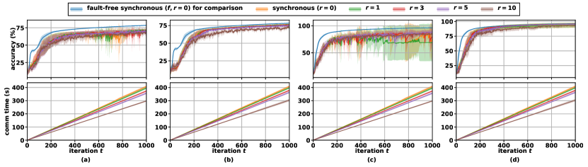
Figure 1: Empirical results for resilient distributed learning tasks with $n=20$, $f=3$, and various $r$’s with Algorithm 1 for Problem DS with D-SGD and CGE gradient filter. Datasets: (ab) Fashion-MNIST, (cd) MNIST. Byzantine faults: (ac) reverse-gradient, (bd) label-flipping. Solid line for average; shade for standard deviation.

5 Empirical studies

In this section, we empirically show the effectiveness of our scheme in Algorithm 1 on some benchmark distributed machine learning tasks. It is worth noting that even though the actual values of redundancy parameter $\epsilon$ are difficult to compute, through the following results we can still see that the said redundancy property exists in real-world scenarios and it supports our algorithm to realize its applicability.

We simulate a server-based distributed learning system using multiple threads, one for the server, the rest for agents, with inter-thread communications handled by message passing interface. The simulator is built in Python with PyTorch [40] and MPI4py [12], and deployed on a virtual machine with 14 vCPUs and 16 GB memory.

The experiments are conducted on two benchmark image-classification datasets: MNIST [6] of monochrome handwritten digits, and Fashion-MNIST [51] of grayscale images of clothes. Each dataset comprises of 60,000 training and 10,000 testing data points in 10 non-overlapping classes, with each image of size $28\times 28$. For each dataset, we train a benchmark neural network LeNet [31] with 431,080 learnable parameters. Data points are divided among agents such that each agent gets 2 out of 10 classes, and each class appears in 4 agents; $\mathcal{D}_{i}$ for each agent $i$ is unique. We show the performance of Algorithm 1 for Problem DS.

In each of our experiments, we simulate a distributed system of $n=20$ agents with $f=3$ and different values of $r=0,1,3,5,10$. Note that when $r=0$, our algorithm becomes the synchronous Problem BS. We also compare these results with the fault-free synchronous Problem AS ($f,r=0$). We choose batch size $b=128$ for D-SGD, and fixed step size $\eta=0.01$. Performance of algorithms is measured by model accuracy at each step. We also document the cumulative communication time of each setting. Experiments of each setting are run 4 times with different random seeds, and the averaged performance is reported. The results are shown in Figure 1. We show the first 1,000 iterations as there is a clear trend of converging by the end of 1,000 iterations for both tasks in all four settings.

For Byzantine agents, we evaluate two types of faults: reverse-gradient where faulty agents reverse the direction of its true gradients, and label-flipping where faulty agents label data points of class $i$ as class $9-i$.

As is shown in the first row of Figure 1, Algorithm 1 converges in a similar rate, and the learned model reaches comparable accuracy to the one learned by synchronous algorithm at the same iteration; there is a gap between them and the fault-free case, echoing the error bound $\mathsf{M}$. In the second row of Figure 1, we see that by dropping out $r$ stragglers, the communication overhead is gradually reduced with increasing value of $r$. It is worth noting that reduction in communication time over $r$ when $r$ is small is more significant than that when $r$ is large, indicating a small number of stragglers work very slow, from which our algorithm improves more in communication overhead.

6 Summary

We studied the impact of $(f,r;\epsilon)$-redundancy in cost functions on resilient distributed optimization and machine learning. Specifically, we presented an algorithm for resilient distributed optimization and learning, and analyzed its convergence when agents’ cost functions have $(f,r;\epsilon)$-redundancy - a generic characterization of redundancy in costs functions. We examined the resilient optimization and learning problem space. We showed that, under $(f,r;\epsilon)$-redundancy, Algorithm 1 with DGD achieves $(f,r;\mathcal{O}(\epsilon))$-resilience for optimization Problems C and D, and Algorithm 1 with D-SGD can solve resilient distributed learning Problems BS, CS, DS with error margins proportional to $\epsilon$. We presented empirical results showing efficacy of Algorithm 1 solving the most generalized Problem DS for resilient distributed learning.

Discussion on limitations Note that our results in this paper are proved under strongly-convex assumptions. One may argue that such kind of assumptions are too strong to be realistic. However, previous research has pointed out that although not a global property, cost functions of many machine learning problems are strongly-convex in the neighborhood of local minimizers [8]. Also, there is a research showing that the results on non-convex cost functions can be derived from those on strongly-convex cost functions [2], and therefore our results can be applied to a broader range of real-world problems. Our empirical results showing efficacy of our algorithm also concur with this argument.

It is also worth noting that the approximation bounds in optimization problems are linearly associated with the number of agents $n$, and the error margins in learning problems are related to $\Gamma$, the size of $\mathcal{W}$. These bounds can be loose when $n$ or $\Gamma$ is large. We do note that in practice $\mathcal{W}$ can be arbitrary, for example, a neighborhood of local minimizers mentioned above, making $\Gamma$ acceptably small. The value of $\epsilon$ can also be small in practice, as indicated by results in Section 5.

Acknowledgements

Research reported in this paper was supported in part by the Army Research Laboratory under Cooperative Agreement W911NF- 17-2-0196, and by the National Science Foundation award 1842198. The views and conclusions contained in this document are those of the authors and should not be interpreted as representing the official policies, either expressed or implied, of the Army Research Laboratory, National Science Foundation, or the U.S. Government. Research reported in this paper is also supported in part by a Fritz Fellowship from Georgetown University.

Appendix A Proofs of theorems in Section 3

In this section, we present the detailed proof of the asymptotic convergence results presented in Section 3, namely Theorems 1, 2, and 3. For each of them, we restate the assumptions, then proceed with the proofs of the theorems.

A.1 Lemma 1

First of all, the proofs of the results presented in Section 3 utilize the following lemma:

Lemma 1.

Consider the general iterative update rule (2). Let $\eta_{t}$ satisfy $$\sum_{t=0}^{\infty}\eta_{t}=\infty~{}\textrm{ and }~{}\sum_{t=0}^{\infty}\eta_{t}^{2}<\infty.$$ For any given gradient aggregation rule $\mathsf{GradAgg}\left(g_{j}^{t}|\,j\in S^{t};n,f,r\right)$, if there exists $\mathsf{M}<\infty$ such that $$\left\lVert\mathsf{GradAgg}\left(g_{j}^{t}|\,j\in S^{t};n,f,r\right)\right\rVert\leq\mathsf{M}$$ (21) for all $t$, and there exists $\mathsf{D}^{*}\in\left[0,\max_{x\in\mathcal{W}}\left\lVert x-x^{*}\right\rVert\right)$ and $\xi>0$ such that when $\left\lVert x^{t}-x^{*}\right\rVert\geq\mathsf{D}^{*}$, $$\phi_{t}\triangleq\left\langle x^{t}-x^{*},\,\mathsf{GradAgg}\left(g_{j}^{t}|\,j\in S^{t};n,f,r\right)\right\rangle\geq\xi,~{}$$ (22) we have $\lim_{t\rightarrow\infty}\left\lVert x^{t}-x^{*}\right\rVert\leq\mathsf{D}^{*}$.

Consider the iterative process (2). Assume that $x^{*}\in\mathcal{W}$. From now on, we use $\mathsf{GradAgg}[t]$ as a short hand for the output of the gradient aggregation rule at iteration $t$, i.e.

$$\mathsf{GradAgg}[t]\triangleq\mathsf{GradAgg}\left(g_{j}^{t}|\,j\in S^{t};n,f,r\right).$$ (23)

The proof of this lemma uses the following sufficient criterion for the convergence of non-negative sequences:

Lemma 2 (Ref. [6]).

Consider a sequence of real values $\{u_{t}\}$, $t=0,1,\dots$. If $u_{t}\geq 0$, $\forall t$,

$$\sum_{t=0}^{\infty}(u_{t+1}-u_{t})_{+}<\infty~{}\textrm{ implies }~{}\left\{\begin{array}[]{l}u_{t}\xrightarrow[t\rightarrow\infty]{}u_{\infty}<\infty,\\ \sum_{t=0}^{\infty}(u_{t+1}-u_{t})_{-}>-\infty,\end{array}\right.$$

where the operators $(\cdot)_{+}$ and $(\cdot)_{-}$ are defined as follows for a real value scalar $x$:

$$(x)_{+}=\left\{\begin{array}[]{ll}x,&x>0,\\ 0,&\textrm{otherwise},\end{array}\right.~{}\textrm{ and }~{}(x)_{-}=\left\{\begin{array}[]{ll}0,&x>0,\\ x,&\textrm{otherwise}.\end{array}\right.$$

A.1.1 Proof of Lemma 1

Let $e_{t}$ denote $\left\lVert x^{t}-x^{*}\right\rVert$. Define a scalar function $\psi$,

$$\psi(y)=\left\{\begin{array}[]{ll}0,&y<\left(\mathsf{D}^{*}\right)^{2},\\ \left(y-\left(\mathsf{D}^{*}\right)^{2}\right)^{2},&\textrm{otherwise}.\end{array}\right.$$ (24)

Let $\psi^{\prime}(y)$ denote the derivative of $\psi$ at $y$. Then (cf. [6])

$$\psi(z)-\psi(y)\leq(z-y)\psi^{\prime}(y)+(z-y)^{2},~{}\forall y,z\in\mathbb{R}_{\geq 0}.$$ (25)

Note,

$$\psi^{\prime}(y)=\max\left\{0,2\left(y-\left(\mathsf{D}^{*}\right)^{2}\right)\right\}.$$ (26)

Now, define

$$h_{t}\triangleq\psi(e_{t}^{2}).$$ (27)

From (25) and (27),

$$h_{t+1}-h_{t}=\psi\left(e_{t+1}^{2}\right)-\psi\left(e_{t}^{2}\right)\leq\left(e_{t+1}^{2}-e_{t}^{2}\right)\psi^{\prime}\left(e_{t}^{2}\right)+\left(e_{t+1}^{2}-e_{t}^{2}\right)^{2},~{}\forall t\in\mathbb{Z}_{\geq 0}.$$ (28)

From now on, we use $\psi_{t}^{\prime}$ as the shorthand for $\psi^{\prime}\left(e_{t}^{2}\right)$, i.e.,

$$\psi_{t}^{\prime}\triangleq\psi^{\prime}\left(e_{t}^{2}\right).$$ (29)

From above, for all $t\geq 0$,

$$h_{t+1}-h_{t}\leq\left(e_{t+1}^{2}-e_{t}^{2}\right)\psi^{\prime}_{t}+\left(e_{t+1}^{2}-e_{t}^{2}\right)^{2}.$$ (30)

Recall the iterative process (2). Using the non-expansion property of Euclidean projection onto a closed convex set,

$$\left\lVert x^{t+1}-x^{*}\right\rVert\leq\left\lVert x^{t}-\eta_{t}\mathsf{GradAgg}[t]-x^{*}\right\rVert.$$ (31)

Taking square on both sides, and recalling that $e_{t}\triangleq\left\lVert x^{t}-x^{*}\right\rVert$,

$$e_{t+1}^{2}\leq e_{t}^{2}-2\eta_{t}\left\langle x_{t}-x^{*},\,\mathsf{GradAgg}[t]\right\rangle+\eta_{t}^{2}\left\lVert\mathsf{GradAgg}[t]\right\rVert^{2}.$$

Recall from (22) that $\left\langle x_{t}-x^{*},\,\mathsf{GradAgg}[t]\right\rangle=\phi_{t}$, therefore,

$$e_{t+1}^{2}\leq e_{t}^{2}-2\eta_{t}\phi_{t}+\eta_{t}^{2}\left\lVert\mathsf{GradAgg}[t]\right\rVert^{2},~{}\forall t\geq 0.$$ (32)

As $\psi^{\prime}_{t}\geq 0,~{}\forall t\in\mathbb{Z}_{\geq 0}$, combining (30) and (32),

$$h_{t+1}-h_{t}\leq\left(-2\eta_{t}\phi_{t}+\eta_{t}^{2}\left\lVert\mathsf{GradAgg}[t]\right\rVert^{2}\right)\psi^{\prime}_{t}+\left(e_{t+1}^{2}-e_{t}^{2}\right)^{2},~{}\forall t\geq 0.$$ (33)

Note that

$$\left\lvert e_{t+1}^{2}-e_{t}^{2}\right\rvert=(e_{t+1}+e_{t})\left\lvert e_{t+1}-e_{t}\right\rvert.$$ (34)

As $\mathcal{W}$ is assumed compact, there exists

$$\Gamma=\max_{x\in\mathcal{W}}\left\lVert x-x^{*}\right\rVert\leq\infty.$$ (35)

Let $\Gamma>0$, since otherwise $\mathcal{W}=\{x^{*}\}$ only contains one point, and the problem becomes trivial. As $x^{t}\in\mathcal{W}$, $\forall t\geq 0$,

$$e_{t}\leq\Gamma,$$ (36)

which implies

$$e_{t+1}+e_{t}\leq 2\Gamma.$$ (37)

Therefore,

$$\left\lvert e_{t+1}^{2}-e_{t}^{2}\right\rvert\leq 2\Gamma\left\lvert e_{t+1}-e_{t}\right\rvert,~{}\forall t\geq 0.$$ (38)

By triangle inequality,

$$\left\lvert e_{t+1}-e_{t}\right\rvert=\left\lvert\left\lVert x^{t+1}-x^{*}\right\rVert-\left\lVert x^{t}-x^{*}\right\rVert\right\rvert\leq\left\lVert x^{t+1}-x^{t}\right\rVert.$$ (39)

From (2) and the non-expansion property of Euclidean projection onto a closed convex set,

$$\left\lVert x^{t+1}-x^{t}\right\rVert=\left\lVert\left[x^{t}-\eta_{t}\mathsf{GradAgg}[t]\right]_{\mathcal{W}}-x^{t}\right\rVert\leq\eta_{t}\left\lVert\mathsf{GradAgg}[t]\right\rVert.$$ (40)

So from (38), (39), and (40),

$$\left\lvert e_{t+1}^{2}-e_{t}^{2}\right\rvert\leq 2\eta_{t}\Gamma\left\lVert\mathsf{GradAgg}[t]\right\rVert,$$

$$\Longrightarrow \left(e_{t+1}^{2}-e_{t}^{2}\right)^{2}\leq 4\eta_{t}^{2}\Gamma^{2}\left\lVert\mathsf{GradAgg}[t]\right\rVert^{2}.$$ (41)

Substituting above in (33),

$$h_{t+1}-h_{t}\leq \left(-2\eta_{t}\phi_{t}+\eta_{t}^{2}\left\lVert\mathsf{GradAgg}[t]\right\rVert^{2}\right)\psi^{\prime}_{t}+4\eta_{t}^{2}\Gamma^{2}\left\lVert\mathsf{GradAgg}[t]\right\rVert^{2},$$

$$= -2\eta_{t}\phi_{t}\psi^{\prime}_{t}+(\psi^{\prime}_{t}+4\Gamma^{2})\eta_{t}^{2}\left\lVert\mathsf{GradAgg}[t]\right\rVert^{2},~{}\forall t\geq 0.$$ (42)

Recall that the statement of Lemma 1 assumes that $\mathsf{D}^{*}\in[0,\max_{x\in\mathcal{W}}\left\lVert x-x^{*}\right\rVert)$, which indicates $\mathsf{D}^{*}<\Gamma$. Using (26) and (36), we have

$$0\leq\psi^{\prime}_{t}\leq 2\left(e_{t}^{2}-\left(\mathsf{D}^{*}\right)^{2}\right)\leq 2\left(\Gamma^{2}-\left(\mathsf{D}^{*}\right)^{2}\right)\leq 2\Gamma^{2}.$$ (43)

Recall from (21) that $\left\lVert\mathsf{GradAgg}[t]\right\rVert\leq\mathsf{M}<\infty$ for all $t$. Substituting (43) in (A.1.1),

$$h_{t+1}-h_{t}\leq -2\eta_{t}\phi_{t}\psi^{\prime}_{t}+(2\Gamma^{2}+4\Gamma^{2})\eta_{t}^{2}\mathsf{M}^{2}=-2\eta_{t}\phi_{t}\psi^{\prime}_{t}+6\Gamma^{2}\eta_{t}^{2}\mathsf{M}^{2},~{}\forall t\geq 0.$$ (44)

Now we use Lemma 2 to show that $h_{\infty}=0$ as follows. For each iteration $t$, consider the following two cases:

Case 1)

Suppose $e_{t}<\mathsf{D}^{*}$. In this case, $\psi^{\prime}_{t}=0$. By Cauchy-Schwartz inequality,

$$\left\lvert\phi_{t}\right\rvert=\left\lvert\left\langle x^{t}-x^{*},\,\mathsf{GradAgg}[t]\right\rangle\right\rvert\leq e_{t}\left\lVert\mathsf{GradAgg}[t]\right\rVert.$$ (45)

By (21) and (36), this implies that

$$\left\lvert\phi_{t}\right\rvert\leq\Gamma\mathsf{M}<\infty.$$ (46)

Thus,

$$\phi_{t}\psi^{\prime}_{t}=0.$$ (47)

Case 2)

Suppose $e_{t}\geq\mathsf{D}^{*}$. Therefore, there exists $\delta\geq 0$, $e_{t}=\mathsf{D}^{*}+\delta$. From (26), we obtain that

$$\psi_{t}^{\prime}=2\left(\left(\mathsf{D}^{*}+\delta\right)^{2}-\left(\mathsf{D}^{*}\right)^{2}\right)=2\delta\left(2\mathsf{D}^{*}+\delta\right).$$ (48)

The statement of Lemma 1 assumes that $\phi_{t}\geq\xi>0$ when $e_{t}\geq\mathsf{D}^{*}$, thus,

$$\phi_{t}\psi^{\prime}_{t}\geq 2\delta\xi\left(2\mathsf{D}^{*}+\delta\right)>0.$$ (49)

From (47) and (49), for both cases,

$$\phi_{t}\psi^{\prime}_{t}\geq 0,~{}\forall t\geq 0.$$ (50)

Combining this with (44),

$$h_{t+1}-h_{t}\leq 6\Gamma^{2}\eta_{t}^{2}\mathsf{M}^{2}.$$ (51)

From above we have

$$\left(h_{t+1}-h_{t}\right)_{+}\leq 6\Gamma^{2}\eta_{t}^{2}\mathsf{M}^{2}.$$ (52)

Since $\sum_{t=0}^{\infty}\eta_{t}^{2}<\infty$, $\Gamma,\mathsf{M}<\infty$,

$$\sum_{t=0}^{\infty}\left(h_{t+1}-h_{t}\right)_{+}\leq 6\Gamma^{2}\mathsf{M}^{2}\sum_{t=0}^{\infty}\eta_{t}^{2}<\infty.$$ (53)

Then Lemma 2 implies that by the definition of $h_{t}$, we have $h_{t}\geq 0,~{}\forall t$,

$$h_{t}\xrightarrow[t\rightarrow\infty]{}h_{\infty}<\infty,~{}\textrm{and}$$ (54)

$$\sum_{t=0}^{\infty}\left(h_{t+1}-h_{t}\right)_{-}>-\infty.$$ (55)

Note that $h_{\infty}-h_{0}=\sum_{t=0}^{\infty}(h_{t+1}-h_{t})$. Thus, from (44) we have

$$h_{\infty}-h_{0}\leq-2\sum_{t=0}^{\infty}\eta_{t}\phi_{t}\psi_{t}^{\prime}+6\Gamma^{2}\mathsf{M}^{2}\sum_{t=0}^{\infty}\eta_{t}^{2}.$$ (56)

By (27) the definition of $h_{t}$, $h_{t}\geq 0$ for all $t$. Therefore, from above we obtain

$$2\sum_{t=0}^{\infty}\eta_{t}\phi_{t}\psi_{t}^{\prime}\leq h_{0}-h_{\infty}+6\Gamma^{2}\mathsf{M}^{2}\sum_{t=0}^{\infty}\eta_{t}^{2}.$$ (57)

By assumption, $\sum_{t=0}^{\infty}\eta_{t}^{2}<\infty$. Substituting from (36) that $e_{t}<\infty$ in (27), we obtain that

$$h_{0}=\psi\left(e_{0}^{2}\right)<\infty.$$ (58)

Therefore, (57) implies that

$$2\sum_{t=0}^{\infty}\eta_{t}\phi_{t}\psi_{t}^{\prime}\leq h_{0}+6\Gamma^{2}\mathsf{M}^{2}\sum_{t=0}^{\infty}\eta_{t}^{2}<\infty.$$ (59)

Or simply,

$$\sum_{t=0}^{\infty}\eta_{t}\phi_{t}\psi_{t}^{\prime}<\infty.$$ (60)

Finally, we reason below by contradiction that $h_{\infty}=0$. Note that for any $\zeta>0$, there exists a unique positive value $\beta$ such that $\zeta=2\beta\left(2\mathsf{D}^{*}+\sqrt{\beta}\right)^{2}$. Suppose that $h_{\infty}=2\beta\left(2\mathsf{D}^{*}+\sqrt{\beta}\right)^{2}$ for some positive value $\beta$. As the sequence $\{h_{t}\}_{t=0}^{\infty}$ converges to $h_{\infty}$ (see (54)), there exists some finite $\tau\in\mathbb{Z}_{\geq 0}$ such that for all $t\geq\tau$,

$$\left\lvert h_{t}-h_{\infty}\right\rvert\leq\beta\left(2\mathsf{D}^{*}+\sqrt{\beta}\right)^{2}$$ (61)

$$\Longrightarrow h_{t}\geq h_{\infty}-\beta\left(2\mathsf{D}^{*}+\sqrt{\beta}\right)^{2}.$$ (62)

As $h_{\infty}=2\beta\left(2\mathsf{D}^{*}+\sqrt{\beta}\right)^{2}$, the above implies that

$$h_{t}\geq\beta\left(2\mathsf{D}^{*}+\sqrt{\beta}\right)^{2},\forall t\geq\tau.$$ (63)

Therefore (cf. (24) and (27)), for all $t\geq\tau$,

$$\left(e_{t}^{2}-\left(\mathsf{D}^{*}\right)^{2}\right)^{2}\geq\beta\left(2\mathsf{D}^{*}+\sqrt{\beta}\right)^{2},\textrm{ or}$$

$$\left\lvert e_{t}^{2}-\left(\mathsf{D}^{*}\right)^{2}\right\rvert\geq\sqrt{\beta}\left(2\mathsf{D}^{*}+\sqrt{\beta}\right).$$

Thus, for each $t\geq\tau$, either

$$e^{2}_{t}\geq\left(\mathsf{D}^{*}\right)^{2}+\sqrt{\beta}\left(2\mathsf{D}^{*}+\sqrt{\beta}\right)=\left(\mathsf{D}^{*}+\sqrt{\beta}\right)^{2},$$ (64)

or

$$e^{2}_{t}\leq\left(\mathsf{D}^{*}\right)^{2}-\sqrt{\beta}\left(2\mathsf{D}^{*}+\sqrt{\beta}\right)<\left(\mathsf{D}^{*}\right)^{2}.$$ (65)

If the latter, i.e., (65) holds true for some $t^{\prime}\geq\tau$,

$$h_{t^{\prime}}=\psi\left(e_{t^{\prime}}^{2}\right)=0,$$ (66)

which contradicts (63). Therefore, (63) implies (64).

From above we obtain that if $h_{\infty}=2\beta\left(2\mathsf{D}^{*}+\sqrt{\beta}\right)^{2}$, there exists $\tau<\infty$ such that for all $t\geq\tau$,

$$e_{t}\geq\mathsf{D}^{*}+\sqrt{\beta}.$$ (67)

Thus, from (49), with $\delta=\sqrt{\beta}$, we obtain that

$$\phi_{t}\psi_{t}^{\prime}\geq 2\xi\sqrt{\beta}\left(2\mathsf{D}^{*}+\sqrt{\beta}\right),\forall t\geq\tau.$$ (68)

Therefore,

$$\sum_{t=\tau}^{\infty}\eta_{t}\phi_{t}\psi_{t}^{\prime}\geq 2\xi\sqrt{\beta}\left(2\mathsf{D}^{*}+\sqrt{\beta}\right)\sum_{t=\tau}^{\infty}\eta_{t}=\infty.$$ (69)

This is a contradiction to (60). Therefore, $h_{\infty}=0$, and by (27), the definition of $h_{t}$,

$$h_{\infty}=\lim_{t\rightarrow\infty}\psi\left(e_{t}^{2}\right)=0.$$ (70)

Hence, by (24), the definition of $\psi(\cdot)$,

$$\lim_{t\rightarrow\infty}\left\lVert x^{t}-x^{*}\right\rVert\leq\mathsf{D}^{*}.$$ (71)

A.2 Proof of Theorem 1

Theorem 1 states the asymptotic convergence of Algorithm 1 when solving Problem C, asynchronous optimization with no Byzantine agents ($f=0,r\geq 0$), using the following gradient aggregator:

$$\textstyle\mathsf{GradAgg}\left(g_{j}^{t}|j\in S^{t};n,f,r\right)=\sum_{j\in{S^{t}}}\nabla Q_{j}(x^{t})$$ (72)

The result is established upon the following assumptions:

Assumption 1. For each (non-faulty) agent $i$, the function $Q_{i}(x)$ is $\mu$-Lipschitz smooth, i.e., $\forall x,x^{\prime}\in\mathbb{R}^{d}$,

$$\left\lVert\nabla Q_{i}(x)-\nabla Q_{i}(x^{\prime})\right\rVert\leq\mu\left\lVert x-x^{\prime}\right\rVert.$$ (73)

Assumption 2. For any set $S\subset[n]$, we define the average cost function to be $Q_{S}(x)=({1}/{\left\lvert S\right\rvert})\sum_{j\in S}Q_{j}(x)$. We assume that $Q_{S}(x)$ is $\gamma$-strongly convex for any $S$ subject to $\left\lvert S\right\rvert\geq n-r$, i.e., $\forall x,x^{\prime}\in\mathbb{R}^{d}$,

$$\left\langle\nabla Q_{S}(x)-\nabla Q_{S}(x^{\prime}),\,x-x^{\prime}\right\rangle\geq\gamma\left\lVert x-x^{\prime}\right\rVert^{2}.$$ (74)

Now we prove Theorem 1. Note that $x^{*}=\arg\min_{x\in\mathcal{W}}\sum_{j\in[n]}Q_{j}(x)$ is the unique minimum of the aggregate cost functions of all agents, and the vector $g_{j}^{t}=\nabla Q_{j}(x^{t})$ is the gradient of $Q_{j}$ at $x^{t}$.

Theorem 1. Suppose that Assumptions 1 and 2 hold true, and the agents’ cost functions satisfy $(0,r;\epsilon)$-redundancy. Assume that $\eta_{t}$ in (2) satisfies $\sum_{t=0}^{\infty}\eta_{t}=\infty$ and $\sum_{t=0}^{\infty}\eta_{t}^{2}<\infty$. Let $\alpha$ and $D$ be defined as follows: $$\alpha\triangleq 1-\frac{r}{n}\cdot\frac{\mu}{\gamma}>0\textrm{ and }D\triangleq\frac{2r\mu}{\alpha\gamma}\epsilon.$$ Then, for the proposed Algorithm 1, $$\lim_{t\rightarrow\infty}\left\lVert x^{t}-x^{*}\right\rVert\leq\mathsf{D},$$ (75) where $x^{*}=\arg\min_{x}\sum_{i\in[n]}Q_{i}(x)$.

Proof.

First, we need to show that $\left\lVert\sum_{j\in S^{t}}\nabla Q_{j}(x^{t})\right\rVert$ is bounded for all $t$. By Assumption 1, for all $j\in[n]$,

$$\left\lVert\nabla Q_{j}(x)-\nabla Q_{j}(x^{*})\right\rVert\leq\mu\left\lVert x-x^{*}\right\rVert.$$ (76)

Let $x_{S}=\arg\min_{x}\sum_{j\in S}Q_{j}(x)$ be the minimum point of the aggregated cost functions of a set $S$ of $n-r$ agents, i.e., $\left\lvert S\right\rvert=n-r$. Note that $\sum_{j\in S}\nabla Q_{j}(x_{S})=0$. By triangle inequality,

$$\left\lVert\sum_{j\in S}\nabla Q_{j}(x_{S})-\sum_{j\in S}\nabla Q_{j}(x^{*})\right\rVert\leq\sum_{j\in S}\left\lVert\nabla Q_{j}(x_{S})-\nabla Q_{j}(x^{*})\right\rVert.$$ (77)

Combining (76) through (77),

$$\left\lVert\sum_{j\in S}\nabla Q_{j}(x^{*})\right\rVert\leq\left\lvert S\right\rvert\mu\left\lVert x_{S}-x^{*}\right\rVert.$$ (78)

By Definition 2 of $(0,r;\epsilon)$-redundancy, $\left\lVert x_{S}-x^{*}\right\rVert\leq\epsilon$. Therefore,

$$\left\lVert\sum_{j\in S}\nabla Q_{j}(x^{*})\right\rVert\leq\mu\epsilon(n-r).$$ (79)

Now, consider an arbitrary agent $i\in[n]\backslash S$. Let $T=S\cup\{i\}$. Using a similar argument as above, we obtain

$$\left\lVert\sum_{j\in T}\nabla Q_{j}(x^{*})\right\rVert\leq\mu\epsilon(n-r+1).$$ (80)

Therefore,

$$\left\lVert\nabla Q_{i}(x^{*})\right\rVert= \left\lVert\sum_{j\in T}\nabla Q_{j}(x^{*})-\sum_{j\in S}\nabla Q_{j}(x^{*})\right\rVert\leq\left\lVert\sum_{j\in T}\nabla Q_{j}(x^{*})\right\rVert+\left\lVert\sum_{j\in S}\nabla Q_{j}(x^{*})\right\rVert$$

$$\leq (n-r)\mu\epsilon+(n-r+1)\mu\epsilon=(2n-2r+1)\mu\epsilon.$$ (81)

Note that the inequality (81) can be applied to any $i\in[n]$ with a suitable choice of $S$ above.

On the other hand, by Assumption 1, for any $x\in\mathbb{R}^{d}$,

$$\left\lVert\nabla Q_{i}(x)-\nabla Q_{i}(x^{*})\right\rVert\leq\mu\left\lVert x-x^{*}\right\rVert.$$ (82)

By triangle inequality,

$$\left\lVert\nabla Q_{i}(x)\right\rVert\leq\left\lVert\nabla Q_{i}(x^{*})\right\rVert+\mu\left\lVert x-x^{*}\right\rVert.$$ (83)

Combining above and (81),

$$\left\lVert\nabla Q_{i}(x)\right\rVert\leq(2n-2r+1)\mu\epsilon+\mu\left\lVert x-x^{*}\right\rVert\leq 2n\mu\epsilon+\mu\left\lVert x-x^{*}\right\rVert.$$ (84)

Recall that $x^{t}\in\mathcal{W}$ for all $t$, where $\mathcal{W}$ is a compact set. There exists a $\Gamma=\max_{x\in\mathcal{W}}\left\lVert x-x^{*}\right\rVert<\infty$, such that $\left\lVert x^{t}-x^{*}\right\rVert\leq\Gamma$ for all $t$. Therefore, for all $t$,

$$\left\lVert\sum_{j\in S^{t}}\nabla Q_{j}(x^{t})\right\rVert =\left\lVert\sum_{j\in S^{t}}\nabla Q_{j}(x^{t})\right\rVert\leq\sum_{j\in S^{t}}\left\lVert\nabla Q_{j}(x^{t})\right\rVert$$

$$\leq\left\lvert S^{t}\right\rvert\cdot\left(2n\mu\epsilon+\mu\left\lVert x^{t}-x^{*}\right\rVert\right)\leq(n-r)\left(2n\mu\epsilon+\mu\Gamma\right)<\infty.$$ (85)

Second, consider the following term $\displaystyle\phi_{t}=\left\langle x^{t}-x^{*},\,\sum_{j\in S^{t}}\nabla Q_{j}(x^{t})\right\rangle$. We have

$$\phi_{t}= \left\langle x^{t}-x^{*},\,\sum_{j\in S^{t}}\nabla Q_{j}(x^{t})\right\rangle$$

$$= \left\langle x^{t}-x^{*},\,\sum_{j\in S^{t}}\nabla Q_{j}(x^{t})+\sum_{k\in[n]\backslash S^{t}}\nabla Q_{k}(x^{t})-\sum_{k\in[n]\backslash S^{t}}\nabla Q_{k}(x^{t})\right\rangle$$

$$= \left\langle x^{t}-x^{*},\,\sum_{j\in[n]}\nabla Q_{j}(x^{t})\right\rangle-\left\langle x^{t}-x^{*},\,\sum_{k\in[n]\backslash S^{t}}\nabla Q_{k}(x^{t})\right\rangle.$$ (86)

For the first term in (A.2), recall that $Q_{S}(x)=\frac{1}{\left\lvert S\right\rvert}\sum_{j\in S}Q_{j}(x)$ for any set $S$ that satisfies $\left\lvert S\right\rvert\geq n-r$. With Assumption 2,

$$\left\langle x^{t}-x^{*},\,\sum_{j\in[n]}\nabla Q_{j}(x^{t})\right\rangle=\left\langle x^{t}-x^{*},\,\sum_{j\in[n]}\nabla Q_{j}(x^{t})-\sum_{j\in[n]}\nabla Q_{j}(x^{*})\right\rangle$$

$$= n\cdot\left\langle x^{t}-x^{*},\,\nabla Q_{[n]}(x^{t})-\nabla Q_{[n]}(x^{*})\right\rangle\geq n\gamma\left\lVert x^{t}-x^{*}\right\rVert^{2}.$$ (87)

For the second term in (A.2), by Cauchy-Schwartz inequality,

$$\left\langle x^{t}-x^{*},\,\sum_{k\in[n]\backslash S^{t}}\nabla Q_{k}(x^{t})\right\rangle =\sum_{k\in[n]\backslash S^{t}}\left\langle x^{t}-x^{*},\,\nabla Q_{k}(x^{t})\right\rangle$$

$$\leq\sum_{k\in[n]\backslash S^{t}}\left\lVert x^{t}-x^{*}\right\rVert\cdot\left\lVert\nabla Q_{k}(x^{t})\right\rVert.$$ (88)

Combining (A.2), (A.2), and (A.2),

$$\phi_{t}\geq n\gamma\left\lVert x^{t}-x^{*}\right\rVert^{2}-\sum_{k\in[n]\backslash S^{t}}\left\lVert x^{t}-x^{*}\right\rVert\left\lVert\nabla Q_{k}(x^{t})\right\rVert.$$ (89)

Substituting from (84) in above, note that $\left\lvert[n]\backslash S^{t}\right\rvert=r$,

$$\phi_{t} \geq n\gamma\left\lVert x^{t}-x^{*}\right\rVert^{2}-\sum_{k\in[n]\backslash S^{t}}\left\lVert x^{t}-x^{*}\right\rVert(2n\mu\epsilon+\mu\left\lVert x^{t}-x^{*}\right\rVert)$$

$$=n\gamma\left\lVert x^{t}-x^{*}\right\rVert^{2}-r\left\lVert x^{t}-x^{*}\right\rVert(2n\mu\epsilon+\mu\left\lVert x^{t}-x^{*}\right\rVert)$$

$$=n\gamma\left(1-\dfrac{r}{n}\cdot\dfrac{\mu}{\gamma}\right)\left\lVert x^{t}-x^{*}\right\rVert\left(\left\lVert x^{t}-x^{*}\right\rVert-\dfrac{2r\mu\epsilon}{\gamma\left(1-\dfrac{r}{n}\cdot\dfrac{\mu}{\gamma}\right)}\right).$$ (90)

Recall that we assume $\displaystyle\alpha=1-\dfrac{r}{n}\cdot\dfrac{\mu}{\gamma}>0$. We have

$$\phi_{t}\geq\alpha n\gamma\left\lVert x^{t}-x^{*}\right\rVert\left(\left\lVert x^{t}-x^{*}\right\rVert-\dfrac{2r\mu}{\alpha\gamma}\epsilon\right).$$ (91)

Let $\mathsf{D}\triangleq\dfrac{2r\mu}{\alpha\gamma}\epsilon$. (91) implies for an arbitrary $\delta>0$,

$$\phi_{t}\geq\alpha n\gamma\delta\left(D+\delta\right)>0~{}\textrm{ when }~{}\left\lVert x^{t}-x^{*}\right\rVert\geq\mathsf{D}+\delta.$$ (92)

Therefore, by Lemma 1,

$$\lim_{t\rightarrow\infty}\left\lVert x^{t}-x^{*}\right\rVert\leq\mathsf{D}.$$ (93)

∎

A.3 Proof of Theorem 2

Theorem 2 states the asymptotic convergence of Algorithm 1 when solving Problem C while using stale gradients. Specifically, we replace (2) in Step 2 of Algorithm 1 with

$$\textstyle x^{t+1}=\left[x^{t}-\eta_{t}\sum_{i=0}^{\tau}\sum_{j\in T^{t;t-i}}\nabla Q_{j}(x^{t-i})\right]_{\mathcal{W}},$$ (94)

where the sets $T^{t;t-i}$’s are defined as follows: (1) $T^{t;t}=S^{t;t}$, and (2) $T^{t;t-i}=S^{t;t-i}\backslash\bigcup_{k=0}^{i-1}T^{t;t-k}$, $\forall i\geq 1$. We further define $T^{t}=\bigcup_{i=0}^{\tau}T^{t;t-i}$. The straggler parameter $\tau\geq 0$ is a predefined integer.

Theorem 2. Suppose Assumption 1 and 2 hold true, and the cost functions of all agents satisfies $(0,r;\epsilon)$-redundancy. Assume that $\eta_{t}$ in (94) satisfies $\sum_{t=0}^{\infty}\eta_{t}=\infty$, $\sum_{t=0}^{\infty}\eta_{t}^{2}<\infty$, and $\eta_{t}\geq\eta_{t+1}$ for all $t$. Let $\alpha$ and $D$ be defined as follows: $$\alpha\triangleq 1-\frac{r}{n}\cdot\frac{\mu}{\gamma}>0\textrm{ and }D\triangleq\frac{2r\mu}{\alpha\gamma}\epsilon.$$ Then, suppose there exists a $\tau\geq 0$ such that $\left\lvert T^{t}\right\rvert\geq n-r$ for all $t$, for the proposed algorithm with update rule (94), $$\lim_{t\rightarrow\infty}\left\lVert x^{t}-x^{*}\right\rVert\leq\mathsf{D},$$ (95) where $x^{*}=\arg\min_{x}\sum_{j\in[n]}Q_{j}(x)$.

The proof consists of three parts. In the first part, we show the norm of the update is bounded for all $t$. In the second part, we consider the inner product term $\phi_{t;1}$ (defined later) is lower-bounded. And in the third part, we show that with a lower-bounded $\phi_{t;1}$ term, the iterative estimate converges.

Proof.

First, we show that $\left\lVert\sum_{i=0}^{\tau}\sum_{j\in T^{t;t-i}}\nabla Q_{j}(x^{t-i})\right\rVert$ is bounded for all $t$. By Assumption 1 and $(0,r;\epsilon)$-redundancy, following the same argument in the proof of Theorem 1, we obtain that for all $j\in[n]$,

$$\left\lVert\nabla Q_{j}(x^{*})\right\rVert\leq(2n-2r+1)\mu\epsilon.$$ (81)

Furthermore, by Assumption 1, for all $x\in\mathbb{R}^{d}$,

$$\left\lVert\nabla Q_{j}(x)\right\rVert\leq 2n\mu\epsilon+\mu\left\lVert x-x^{*}\right\rVert.$$ (84)

Recall that $x^{t}\in\mathcal{W}$ for all $t$, where $\mathcal{W}$ is a compact set. There exists a $\Gamma=\max_{x\in\mathcal{W}}\left\lVert x-x^{*}\right\rVert<\infty$, such that $\left\lVert x^{t}-x^{*}\right\rVert\leq\Gamma$ for all $t$. Therefore, for all $t$,

$$\left\lVert\sum_{i=0}^{\tau}\sum_{j\in T^{t;t-i}}\nabla Q_{j}(x^{t-i})\right\rVert\leq\sum_{i=0}^{\tau}\sum_{j\in T^{t;t-i}}\left\lVert\nabla Q_{j}(x^{t-i})\right\rVert$$

$$\leq \sum_{i=0}^{\tau}\left\lvert T^{t;t-i}\right\rvert\cdot(2n\mu\epsilon+\mu\left\lVert x^{t-i}-x^{*}\right\rVert)\leq\sum_{i=0}^{\tau}\left\lvert T^{t;t-i}\right\rvert\cdot(2n\mu\epsilon+\mu\Gamma)$$ (96)

Recall the definition of $T^{t;t-i}$, that $T^{t;t-i_{1}}\cap T^{t;t-i_{2}}=\varnothing$ for all $0\leq i_{1},i_{2}\leq\tau$, $i_{1}\neq i_{2}$. Therefore, $\sum_{i=0}^{\tau}\left\lvert T^{t;t-i}\right\rvert\leq n$. Thus,

$$\left\lVert\sum_{i=0}^{\tau}\sum_{j\in T^{t;t-i}}\nabla Q_{j}(x^{t-i})\right\rVert\leq n(2n\mu\epsilon+\mu\Gamma)<\infty.$$ (97)

Second, consider the term

$$\phi_{t}=\left\langle x^{t}-x^{*},\,\sum_{i=0}^{\tau}\sum_{j\in T^{t;t-i}}\nabla Q_{j}(x^{t-i})\right\rangle.$$ (98)

Note that with the non-expansion property of Euclidean projection onto a closed convex set we have

$$\left\lVert x^{t+1}-x^{*}\right\rVert =\left\lVert x^{t}-\eta_{t}\sum_{i=0}^{\tau}\sum_{j\in T^{t;t-i}}\nabla Q_{j}(x^{t-i})-x^{*}\right\rVert^{2}$$

$$\leq\left\lVert x^{t}-x^{*}\right\rVert^{2}-2\eta_{t}\phi_{t}+\eta_{t}^{2}\left\lVert\sum_{i=0}^{\tau}\sum_{j\in T^{t;t-i}}\nabla Q_{j}(x^{t-i})\right\rVert^{2}.$$ (99)

Let $T^{t}=\bigcup_{i=0}^{\tau}T^{t;t-i}$ be the set of agents whose gradients are used for the update at iteration $t$.

$$\sum_{i=0}^{\tau}\sum_{j\in T^{t;t-i}}\nabla Q_{j}(x^{t-i})= \sum_{i=0}^{\tau}\sum_{j\in T^{t;t-i}}\left(\nabla Q_{j}(x^{t})-\nabla Q_{j}(x^{t})+\nabla Q_{j}(x^{t-i})\right)$$

$$= \sum_{i=0}^{\tau}\sum_{j\in T^{t;t-i}}\nabla Q_{j}(x^{t})-\sum_{i=0}^{\tau}\sum_{j\in T^{t;t-i}}\left(\nabla Q_{j}(x^{t})-\nabla Q_{j}(x^{t-i})\right)$$

$$= \sum_{j\in T^{t}}\nabla Q_{j}(x^{t})-\sum_{i=0}^{\tau}\sum_{j\in T^{t;t-i}}\left(\nabla Q_{j}(x^{t})-\nabla Q_{j}(x^{t-i})\right).$$ (100)

Therefore, we have

$$\phi_{t}= \left\langle x^{t}-x^{*},\,\sum_{i=0}^{\tau}\sum_{j\in T^{t;t-i}}\nabla Q_{j}(x^{t-i})\right\rangle$$

$$= \left\langle x^{t}-x^{*},\,\sum_{j\in T^{t}}\nabla Q_{j}(x^{t})\right\rangle-\left\langle x^{t}-x^{*},\,\sum_{i=0}^{\tau}\sum_{j\in T^{t;t-i}}\left(\nabla Q_{j}(x^{t})-\nabla Q_{j}(x^{t-i})\right)\right\rangle.$$ (101)

For the first term in (A.3), denote it $\phi_{t;1}$, we have

$$\phi_{t;1}= \left\langle x^{t}-x^{*},\,\sum_{j\in T^{t}}\nabla Q_{j}(x^{t})\right\rangle$$

$$= \left\langle x^{t}-x^{*},\,\sum_{j\in T^{t}}\nabla Q_{j}(x^{t})+\sum_{k\in[n]\backslash T^{t}}\nabla Q_{k}(x^{t})-\sum_{k\in[n]\backslash T^{t}}\nabla Q_{k}(x^{t})\right\rangle$$

$$= \left\langle x^{t}-x^{*},\,\sum_{j\in[n]}\nabla Q_{j}(x^{t})\right\rangle-\left\langle x^{t}-x^{*},\,\sum_{k\in[n]\backslash T^{t}}\nabla Q_{k}(x^{t})\right\rangle.$$ (102)

Recall (A.2) and (A.2), we have the same result as we have in (89):

$$\phi_{t;1}\geq n\gamma\left\lVert x^{t}-x^{*}\right\rVert^{2}-\sum_{k\in[n]\backslash T^{t}}\left\lVert x^{t}-x^{*}\right\rVert\left\lVert\nabla Q_{k}(x^{t})\right\rVert.$$ (103)

Note that $\left\lvert T^{t}\right\rvert\geq n-r$, or $\left\lvert[n]\backslash T^{t}\right\rvert\leq r$. Combining above and (84),

$$\phi_{t;1}\geq n\gamma\left\lVert x^{t}-x^{*}\right\rVert^{2}-r\left\lVert x^{t}-x^{*}\right\rVert\left(2n\mu\epsilon+\mu\left\lVert x-x^{*}\right\rVert\right)$$

$$= n\gamma\left(1-\dfrac{r}{n}\cdot\dfrac{\mu}{\gamma}\right)\left\lVert x^{t}-x^{*}\right\rVert\left(\left\lVert x^{t}-x^{*}\right\rVert-\dfrac{2r\mu\epsilon}{\gamma\left(1-\dfrac{r}{n}\cdot\dfrac{\mu}{\gamma}\right)}\right).$$ (104)

Recall that we assume $\displaystyle\alpha=1-\dfrac{r}{n}\cdot\dfrac{\mu}{\gamma}>0$. We have

$$\phi_{t;1}\geq\alpha n\gamma\left\lVert x^{t}-x^{*}\right\rVert\left(\left\lVert x^{t}-x^{*}\right\rVert-\dfrac{2r\mu}{\alpha\gamma}\epsilon\right).$$ (105)

Let $\mathsf{D}\triangleq\dfrac{2r\mu}{\alpha\gamma}\epsilon$. (105) implies for an arbitrary $\delta>0$,

$$\phi_{t;1}\geq\alpha n\gamma\delta\left(D+\delta\right)>0~{}\textrm{ when }~{}\left\lVert x^{t}-x^{*}\right\rVert\geq\mathsf{D}+\delta.$$ (106)

For the second term in (A.3), denote it $\phi_{t;2}$, by Cauchy-Schwartz inequality, we have

$$\phi_{t;2}= \left\langle x^{t}-x^{*},\,\sum_{i=0}^{\tau}\sum_{j\in T^{t;t-i}}\left(\nabla Q_{j}(x^{t})-\nabla Q_{j}(x^{t-i})\right)\right\rangle$$

$$\leq \left\lVert x^{t}-x^{*}\right\rVert\cdot\left\lVert\sum_{i=0}^{\tau}\sum_{j\in T^{t;t-i}}\left(\nabla Q_{j}(x^{t})-\nabla Q_{j}(x^{t-i})\right)\right\rVert.$$ (107)

Consider the factor $\left\lVert\sum_{i=0}^{t}\sum_{j\in T^{t;t-i}}\left(\nabla Q_{j}(x^{t})-\nabla Q_{j}(x^{t-i})\right)\right\rVert$. By triangle inequality,

$$\left\lVert\sum_{i=0}^{\tau}\sum_{j\in T^{t;t-i}}\left(\nabla Q_{j}(x^{t})-\nabla Q_{j}(x^{t-i})\right)\right\rVert\leq \sum_{i=0}^{\tau}\sum_{j\in T^{t;t-i}}\left\lVert\nabla Q_{j}(x^{t})-\nabla Q_{j}(x^{t-i})\right\rVert.$$ (108)

By Assumption 1 and $x^{t}\in\mathcal{W}$ for all $t$,

$$\left\lVert\nabla Q_{j}(x^{t})-\nabla Q_{j}(x^{t-i})\right\rVert\leq\mu\left\lVert x^{t}-x^{t-i}\right\rVert.$$ (109)

According to the update rule (94),

$$x^{t} =x^{t-1}-\eta_{t-1}\sum_{h=0}^{\tau}\sum_{j\in T^{t-1;t-1-h}}\nabla Q_{j}(x^{t-1-h})$$

$$=x^{t-2}-\eta_{t-1}\sum_{h=0}^{\tau}\sum_{j\in T^{t-1;t-1-h}}\nabla Q_{j}(x^{t-1-h})-\eta_{t-2}\sum_{h=0}^{\tau}\sum_{j\in T^{t-2;t-2-h}}\nabla Q_{j}(x^{t-2-h})$$

$$=x^{t-2}-\sum_{k=1}^{2}\eta_{t-k}\sum_{h=0}^{\tau}\sum_{j\in T^{t-k;t-k-h}}\nabla Q_{j}(x^{t-k-h})$$

$$=\cdots$$

$$=x^{t-i}-\sum_{k=1}^{i}\eta_{t-k}\sum_{h=0}^{\tau}\sum_{j\in T^{t-k;t-k-h}}\nabla Q_{j}(x^{t-k-h}).$$ (110)

Therefore,

$$\left\lVert x^{t}-x^{t-i}\right\rVert= \left\lVert\sum_{k=1}^{i}\eta_{t-k}\sum_{h=0}^{\tau}\sum_{j\in T^{t-k;t-k-h}}\nabla Q_{j}(x^{t-k-h})\right\rVert$$

$$\leq \sum_{k=1}^{i}\eta_{t-k}\left\lVert\sum_{h=0}^{\tau}\sum_{j\in T^{t-k;t-k-h}}\nabla Q_{j}(x^{t-k-h})\right\rVert.$$ (111)

By (97), let $\overline{G}=n(2n\mu\epsilon+\mu\Gamma)$. Also note that for all $t$, $\eta_{t}\geq\eta_{t+1}$. From above we have

$$\left\lVert x^{t}-x^{t-i}\right\rVert\leq\sum_{k=1}^{i}\eta_{t-k}\overline{G}\leq i\cdot\eta_{t-i}\overline{G}.$$ (112)

Combining (108), (109) and above, we have

$$\left\lVert\sum_{i=0}^{\tau}\sum_{j\in T^{t;t-i}}\left(\nabla Q_{j}(x^{t})-\nabla Q_{j}(x^{t-i})\right)\right\rVert\leq\sum_{i=0}^{\tau}\sum_{j\in T^{t;t-i}}\left\lVert\nabla Q_{j}(x^{t})-\nabla Q_{j}(x^{t-i})\right\rVert$$

$$\leq \sum_{i=0}^{\tau}\sum_{j\in T^{t;t-i}}\mu i\cdot\eta_{t-i}\overline{G}\leq\overline{G}\cdot\sum_{i=0}^{\tau}\sum_{j\in T^{t;t-i}}\mu\tau\eta_{t-\tau}=\overline{G}\cdot\sum_{j\in T^{t}}\mu\tau\eta_{t-\tau}$$

$$\leq \mu\tau\eta_{t-\tau}n\overline{G}.$$ (113)

Combining with (A.3), from above we have

$$\phi_{t;2}\leq\mu\tau\eta_{t-\tau}n\overline{G}\left\lVert x^{t}-x^{*}\right\rVert.$$ (114)

In summary, $\phi_{t}=\phi_{t;1}-\phi_{t;2}$.

Third, we show that assuming that there exists some $\mathsf{D}^{*}\in[0,\max_{x\in\mathcal{W}}\left\lVert x-x^{*}\right\rVert)$ and $\xi>0$, such that $\phi_{t;1}\geq\xi$ when $\left\lVert x^{t}-x^{*}\right\rVert\geq\mathsf{D}^{*}$, we have $\lim_{t\rightarrow\infty}\left\lVert x^{t}-x^{*}\right\rVert\leq\mathsf{D}^{*}$.

Let $e^{t}$ denote $\left\lVert x^{t}-x^{*}\right\rVert$. Define a scalar function $\psi$,

$$\psi(y)=\left\{\begin{array}[]{ll}0,&y<\left(\mathsf{D}^{*}\right)^{2},\\ \left(y-\left(\mathsf{D}^{*}\right)^{2}\right)^{2},&\textrm{otherwise}.\end{array}\right.$$ (115)

Let $\psi^{\prime}(y)$ denote the derivative of $\psi$ at $y$. Then (cf. [6])

$$\psi(z)-\psi(y)\leq(z-y)\psi^{\prime}(y)+(z-y)^{2},~{}\forall y,z\in\mathbb{R}_{\geq 0}.$$ (116)

Note,

$$\psi^{\prime}(y)=\max\left\{0,2\left(y-\left(\mathsf{D}^{*}\right)^{2}\right)\right\}.$$ (117)

Now, define

$$h_{t}\triangleq\psi(e_{t}^{2}).$$ (118)

From (116) and (118),

$$h_{t+1}-h_{t}=\psi\left(e_{t+1}^{2}\right)-\psi\left(e_{t}^{2}\right)\leq\left(e_{t+1}^{2}-e_{t}^{2}\right)\psi^{\prime}\left(e_{t}^{2}\right)+\left(e_{t+1}^{2}-e_{t}^{2}\right)^{2},~{}\forall t\in\mathbb{Z}_{\geq 0}.$$ (119)

From now on, we use $\psi_{t}^{\prime}$ as the shorthand for $\psi^{\prime}\left(e_{t}^{2}\right)$, i.e.,

$$\psi_{t}^{\prime}\triangleq\psi^{\prime}\left(e_{t}^{2}\right).$$ (120)

From above, for all $t\geq 0$,

$$h_{t+1}-h_{t}\leq\left(e_{t+1}^{2}-e_{t}^{2}\right)\psi^{\prime}_{t}+\left(e_{t+1}^{2}-e_{t}^{2}\right)^{2}.$$ (121)

Recall the iterative process (94). From now on, we use $\mathsf{StragAgg}[t]$ as a short hand for the output of the gradient aggregation rule at iteration $t$, i.e.

$$\mathsf{StragAgg}[t]\triangleq\sum_{i=0}^{\tau}\sum_{j\in T^{t;t-i}}\nabla Q_{j}(x^{t-i}).$$ (122)

Using the non-expansion property of Euclidean projection onto a closed convex set,

$$\left\lVert x^{t+1}-x^{*}\right\rVert\leq\left\lVert x^{t}-\eta_{t}\mathsf{StragAgg}[t]-x^{*}\right\rVert.$$ (123)

Taking square on both sides,

$$e_{t+1}^{2}\leq e_{t}^{2}-2\eta_{t}\left\langle x_{t}-x^{*},\,\mathsf{StragAgg}[t]\right\rangle+\eta_{t}^{2}\left\lVert\mathsf{StragAgg}[t]\right\rVert^{2}.$$

Recall from (98) that $\left\langle x_{t}-x^{*},\,\mathsf{StragAgg}[t]\right\rangle=\phi_{t}$, therefore (cf. (A.3)),

$$e_{t+1}^{2}\leq e_{t}^{2}-2\eta_{t}\phi_{t}+\eta_{t}^{2}\left\lVert\mathsf{StragAgg}[t]\right\rVert^{2},~{}\forall t\geq 0.$$ (124)

As $\psi^{\prime}_{t}\geq 0,~{}\forall t\in\mathbb{Z}_{\geq 0}$, combining (121) and (124),

$$h_{t+1}-h_{t}\leq\left(-2\eta_{t}\phi_{t}+\eta_{t}^{2}\left\lVert\mathsf{StragAgg}[t]\right\rVert^{2}\right)\psi^{\prime}_{t}+\left(e_{t+1}^{2}-e_{t}^{2}\right)^{2},~{}\forall t\geq 0.$$ (125)

Note that

$$\left\lvert e_{t+1}^{2}-e_{t}^{2}\right\rvert=(e_{t+1}+e_{t})\left\lvert e_{t+1}-e_{t}\right\rvert.$$ (126)

As $\mathcal{W}$ is assumed compact, there exists

$$\Gamma=\max_{x\in\mathcal{W}}\left\lVert x-x^{*}\right\rVert\leq\infty.$$ (127)

Let $\Gamma>0$, since otherwise $\mathcal{W}=\{x^{*}\}$ only contains one point, and the problem becomes trivial. As $x^{t}\in\mathcal{W}$, $\forall t\geq 0$,

$$e_{t}\leq\Gamma,$$ (128)

which implies

$$e_{t+1}+e_{t}\leq 2\Gamma.$$ (129)

Therefore,

$$\left\lvert e_{t+1}^{2}-e_{t}^{2}\right\rvert\leq 2\Gamma\left\lvert e_{t+1}-e_{t}\right\rvert,~{}\forall t\geq 0.$$ (130)

By triangle inequality,

$$\left\lvert e_{t+1}-e_{t}\right\rvert=\left\lvert\left\lVert x^{t+1}-x^{*}\right\rVert-\left\lVert x^{t}-x^{*}\right\rVert\right\rvert\leq\left\lVert x^{t+1}-x^{t}\right\rVert.$$ (131)

From (94) and the non-expansion property of Euclidean projection onto a closed convex set,

$$\left\lVert x^{t+1}-x^{t}\right\rVert=\left\lVert\left[x^{t}-\eta_{t}\mathsf{StragAgg}[t]\right]_{\mathcal{W}}-x^{t}\right\rVert\leq\eta_{t}\left\lVert\mathsf{StragAgg}[t]\right\rVert.$$ (132)

So from (130), (131), and (132),

$$\left\lvert e_{t+1}^{2}-e_{t}^{2}\right\rvert\leq 2\eta_{t}\Gamma\left\lVert\mathsf{StragAgg}[t]\right\rVert,$$

$$\Longrightarrow \left(e_{t+1}^{2}-e_{t}^{2}\right)^{2}\leq 4\eta_{t}^{2}\Gamma^{2}\left\lVert\mathsf{StragAgg}[t]\right\rVert^{2}.$$ (133)

Substituting above in (125),

$$h_{t+1}-h_{t}\leq \left(-2\eta_{t}\phi_{t}+\eta_{t}^{2}\left\lVert\mathsf{StragAgg}[t]\right\rVert^{2}\right)\psi^{\prime}_{t}+4\eta_{t}^{2}\Gamma^{2}\left\lVert\mathsf{StragAgg}[t]\right\rVert^{2},$$

$$= -2\eta_{t}\phi_{t}\psi^{\prime}_{t}+(\psi^{\prime}_{t}+4\Gamma^{2})\eta_{t}^{2}\left\lVert\mathsf{StragAgg}[t]\right\rVert^{2},~{}\forall t\geq 0.$$ (134)

Recall that $\phi_{t}=\phi_{t;1}-\phi_{t;2}$. Also, $\eta_{t}\geq\eta_{t+1}$ for all $t$. Substitute for (128) and (114) in above, we obtain that

$$h_{t+1}-h_{t}\leq -2\eta_{t}(\phi_{t;1}-\phi_{t;2})\psi^{\prime}_{t}+(\psi^{\prime}_{t}+4\Gamma^{2})\eta_{t}^{2}\left\lVert\mathsf{StragAgg}[t]\right\rVert^{2},~{}\forall t\geq 0$$

$$\leq -2\eta_{t}\phi_{t;1}\psi^{\prime}_{t}+2\eta_{t}(\mu\tau\eta_{t-\tau}n\overline{G}e_{t})\psi^{\prime}_{t}+(\psi^{\prime}_{t}+4\Gamma^{2})\eta_{t}^{2}\left\lVert\mathsf{StragAgg}[t]\right\rVert^{2},~{}\forall t\geq 0$$

$$\leq -2\eta_{t}\phi_{t;1}\psi^{\prime}_{t}+2\eta_{t}^{2}\mu\tau n\overline{G}\Gamma\psi^{\prime}_{t}+(\psi^{\prime}_{t}+4\Gamma^{2})\eta_{t}^{2}\left\lVert\mathsf{StragAgg}[t]\right\rVert^{2},~{}\forall t\geq 0.$$ (135)

Let us assume for now that $\mathsf{D}^{*}\in[0,\max_{x\in\mathcal{W}}\left\lVert x-x^{*}\right\rVert)$, which indicates $\mathsf{D}^{*}<\Gamma$. Using (117) and (128), we have

$$0\leq\psi^{\prime}_{t}\leq 2\left(e_{t}^{2}-\left(\mathsf{D}^{*}\right)^{2}\right)\leq 2\left(\Gamma^{2}-\left(\mathsf{D}^{*}\right)^{2}\right)\leq 2\Gamma^{2}.$$ (136)

From (97) (recall that $\overline{G}=n(2n\mu\epsilon+\mu\Gamma)$), $\left\lVert\mathsf{StragAgg}[t]\right\rVert\leq\overline{G}<\infty$ for all $t$. Substituting (136) in (A.3),

$$h_{t+1}-h_{t}\leq -2\eta_{t}\phi_{t;1}\psi^{\prime}_{t}+2\eta_{t}^{2}\mu\tau n\overline{G}\Gamma\left(2\Gamma^{2}\right)+\left(2\Gamma^{2}+4\Gamma^{2}\right)\eta_{t}^{2}\overline{G}^{2}$$

$$= -2\eta_{t}\phi_{t;1}\psi^{\prime}_{t}+\eta_{t}^{2}\left(4\mu\tau n\Gamma^{3}\overline{G}+6\Gamma^{2}\overline{G}^{2}\right),~{}\forall t\geq 0.$$ (137)

Now we use Lemma 2 to show that $h_{\infty}=0$ as follows. For each iteration $t$, consider the following two cases:

Case 1)

Suppose $e_{t}<\mathsf{D}^{*}$. In this case, $\psi^{\prime}_{t}=0$. By Cauchy-Schwartz inequality,

$$\left\lvert\phi_{t;1}\right\rvert=\left\lvert\left\langle x^{t}-x^{*},\,\mathsf{StragAgg}[t]\right\rangle\right\rvert\leq e_{t}\left\lVert\mathsf{StragAgg}[t]\right\rVert.$$ (138)

By (97) and (128), this implies that

$$\left\lvert\phi_{t;1}\right\rvert\leq\Gamma\overline{G}<\infty.$$ (139)

Thus,

$$\phi_{t;1}\psi^{\prime}_{t}=0.$$ (140)

Case 2)

Suppose $e_{t}\geq\mathsf{D}^{*}$. Therefore, there exists $\delta\geq 0$, $e_{t}=\mathsf{D}^{*}+\delta$. From (117), we obtain that

$$\psi_{t}^{\prime}=2\left(\left(\mathsf{D}^{*}+\delta\right)^{2}-\left(\mathsf{D}^{*}\right)^{2}\right)=2\delta\left(2\mathsf{D}^{*}+\delta\right).$$ (141)

The statement of Lemma 1 assumes that $\phi_{t}\geq\xi>0$ when $e_{t}\geq\mathsf{D}^{*}$, thus,

$$\phi_{t;1}\psi^{\prime}_{t}\geq 2\delta\xi\left(2\mathsf{D}^{*}+\delta\right)>0.$$ (142)

From (140) and (142), for both cases,

$$\phi_{t;1}\psi^{\prime}_{t}\geq 0,~{}\forall t\geq 0.$$ (143)

Combining this with (A.3),

$$h_{t+1}-h_{t}\leq\eta_{t}^{2}\left(4\mu\tau n\Gamma^{3}\overline{G}+6\Gamma^{2}\overline{G}^{2}\right).$$ (144)

From above we have

$$\left(h_{t+1}-h_{t}\right)_{+}\leq\eta_{t}^{2}\left(4\mu\tau n\Gamma^{3}\overline{G}+6\Gamma^{2}\overline{G}^{2}\right).$$ (145)

Since $\sum_{t=0}^{\infty}\eta_{t}^{2}<\infty$, $\Gamma,\overline{G}<\infty$,

$$\sum_{t=0}^{\infty}\left(h_{t+1}-h_{t}\right)_{+}\leq\left(4\mu\tau n\Gamma^{3}\overline{G}+6\Gamma^{2}\overline{G}^{2}\right)\sum_{t=0}^{\infty}\eta_{t}^{2}<\infty.$$ (146)

Then Lemma 2 implies that by the definition of $h_{t}$, we have $h_{t}\geq 0,~{}\forall t$,

$$h_{t}\xrightarrow[t\rightarrow\infty]{}h_{\infty}<\infty,~{}\textrm{and}$$ (147)

$$\sum_{t=0}^{\infty}\left(h_{t+1}-h_{t}\right)_{-}>-\infty.$$ (148)

Note that $h_{\infty}-h_{0}=\sum_{t=0}^{\infty}(h_{t+1}-h_{t})$. Thus, from (A.3) we have

$$h_{\infty}-h_{0}\leq-2\sum_{t=0}^{\infty}\eta_{t}\phi_{t;1}\psi_{t}^{\prime}+\left(4\mu\tau n\Gamma^{3}\overline{G}+6\Gamma^{2}\overline{G}^{2}\right)\sum_{t=0}^{\infty}\eta_{t}^{2}.$$ (149)

By (27) the definition of $h_{t}$, $h_{t}\geq 0$ for all $t$. Therefore, from above we obtain

$$2\sum_{t=0}^{\infty}\eta_{t}\phi_{t;1}\psi_{t}^{\prime}\leq h_{0}-h_{\infty}+\left(4\mu\tau n\Gamma^{3}\overline{G}+6\Gamma^{2}\overline{G}^{2}\right)\sum_{t=0}^{\infty}\eta_{t}^{2}.$$ (150)

By assumption, $\sum_{t=0}^{\infty}\eta_{t}^{2}<\infty$. Substituting from (128) that $e_{t}<\infty$ in (118), we obtain that

$$h_{0}=\psi\left(e_{0}^{2}\right)<\infty.$$ (151)

Therefore, (150) implies that

$$2\sum_{t=0}^{\infty}\eta_{t}\phi_{t;1}\psi_{t}^{\prime}\leq h_{0}+\left(4\mu\tau n\Gamma^{3}\overline{G}+6\Gamma^{2}\overline{G}^{2}\right)\sum_{t=0}^{\infty}\eta_{t}^{2}<\infty.$$ (152)

Or simply,

$$\sum_{t=0}^{\infty}\eta_{t}\phi_{t;1}\psi_{t}^{\prime}<\infty.$$ (153)

Finally, we reason below by contradiction that $h_{\infty}=0$. Note that for any $\zeta>0$, there exists a unique positive value $\beta$ such that $\zeta=2\beta\left(2\mathsf{D}^{*}+\sqrt{\beta}\right)^{2}$. Suppose that $h_{\infty}=2\beta\left(2\mathsf{D}^{*}+\sqrt{\beta}\right)^{2}$ for some positive value $\beta$. As the sequence $\{h_{t}\}_{t=0}^{\infty}$ converges to $h_{\infty}$ (see (147)), there exists some finite $\tau\in\mathbb{Z}_{\geq 0}$ such that for all $t\geq\tau$,

$$\left\lvert h_{t}-h_{\infty}\right\rvert\leq\beta\left(2\mathsf{D}^{*}+\sqrt{\beta}\right)^{2}$$ (154)

$$\Longrightarrow h_{t}\geq h_{\infty}-\beta\left(2\mathsf{D}^{*}+\sqrt{\beta}\right)^{2}.$$ (155)

As $h_{\infty}=2\beta\left(2\mathsf{D}^{*}+\sqrt{\beta}\right)^{2}$, the above implies that

$$h_{t}\geq\beta\left(2\mathsf{D}^{*}+\sqrt{\beta}\right)^{2},\forall t\geq\tau.$$ (156)

Therefore (cf. (115) and (118)), for all $t\geq\tau$,

$$\left(e_{t}^{2}-\left(\mathsf{D}^{*}\right)^{2}\right)^{2}\geq\beta\left(2\mathsf{D}^{*}+\sqrt{\beta}\right)^{2},\textrm{ or}$$

$$\left\lvert e_{t}^{2}-\left(\mathsf{D}^{*}\right)^{2}\right\rvert\geq\sqrt{\beta}\left(2\mathsf{D}^{*}+\sqrt{\beta}\right).$$

Thus, for each $t\geq\tau$, either

$$e^{2}_{t}\geq\left(\mathsf{D}^{*}\right)^{2}+\sqrt{\beta}\left(2\mathsf{D}^{*}+\sqrt{\beta}\right)=\left(\mathsf{D}^{*}+\sqrt{\beta}\right)^{2},$$ (157)

or

$$e^{2}_{t}\leq\left(\mathsf{D}^{*}\right)^{2}-\sqrt{\beta}\left(2\mathsf{D}^{*}+\sqrt{\beta}\right)<\left(\mathsf{D}^{*}\right)^{2}.$$ (158)

If the latter, i.e., (158) holds true for some $t^{\prime}\geq\tau$,

$$h_{t^{\prime}}=\psi\left(e_{t^{\prime}}^{2}\right)=0,$$ (159)

which contradicts (156). Therefore, (156) implies (157).

From above we obtain that if $h_{\infty}=2\beta\left(2\mathsf{D}^{*}+\sqrt{\beta}\right)^{2}$, there exists $\tau<\infty$ such that for all $t\geq\tau$,

$$e_{t}\geq\mathsf{D}^{*}+\sqrt{\beta}.$$ (160)

Thus, from (142), with $\delta=\sqrt{\beta}$, we obtain that

$$\phi_{t}\psi_{t}^{\prime}\geq 2\xi\sqrt{\beta}\left(2\mathsf{D}^{*}+\sqrt{\beta}\right),\forall t\geq\tau.$$ (161)

Therefore,

$$\sum_{t=\tau}^{\infty}\eta_{t}\phi_{t}\psi_{t}^{\prime}\geq 2\xi\sqrt{\beta}\left(2\mathsf{D}^{*}+\sqrt{\beta}\right)\sum_{t=\tau}^{\infty}\eta_{t}=\infty.$$ (162)

This is a contradiction to (153). Therefore, $h_{\infty}=0$, and by (118), the definition of $h_{t}$,

$$h_{\infty}=\lim_{t\rightarrow\infty}\psi\left(e_{t}^{2}\right)=0.$$ (163)

Hence, by (115), the definition of $\psi(\cdot)$,

$$\lim_{t\rightarrow\infty}\left\lVert x^{t}-x^{*}\right\rVert\leq\mathsf{D}^{*}.$$ (164)

Finally, recall the result in (106), for arbitrary $\delta>0$,

$$\phi_{t;1}\geq\alpha n\gamma\delta\left(D+\delta\right)>0~{}\textrm{ when }~{}\left\lVert x^{t}-x^{*}\right\rVert\geq\mathsf{D}+\delta,$$ (106)

with $\displaystyle\alpha=1-\dfrac{r}{n}\cdot\dfrac{\mu}{\gamma}>0$ and $\mathsf{D}=\dfrac{2r\mu}{\alpha\gamma}\epsilon$. Combining with the third part of this proof, $\lim_{t\rightarrow\infty}\left\lVert x^{t}-x^{*}\right\rVert\leq\mathsf{D}$. ∎

A.4 Proof of Theorems 3 and the special case when using CGE gradient filter

Theorem 3 states the asymptotic convergence of Algorithm 1 when solving Problem D, asynchronous Byzantine fault-tolerant optimization ($f,r\geq 0$), using the following gradient aggregator:

$$\textstyle\mathsf{GradAgg}\left(g_{j}^{t}|j\in S^{t};n,f,r\right)=\mathsf{GradFilter}\left(g_{j}^{t}|j\in S^{t};n-r,f\right).$$ (165)

i.e., any gradient filter that satisfies the condition listed in the theorem. The result is established upon Assumption 1 and the following assumption:

Assumption 3. For any set $S\subset\mathcal{H}$, we define the average cost function to be $Q_{S}(x)=({1}/{\left\lvert S\right\rvert})\sum_{j\in S}Q_{j}(x)$. We assume that $Q_{S}(x)$ is $\gamma$-strongly convex for any $S$ subject to $\left\lvert S\right\rvert\geq n-f$, i.e., $\forall x,x^{\prime}\in\mathbb{R}^{d}$,

$$\left\langle\nabla Q_{S}(x)-\nabla Q_{S}(x^{\prime}),\,x-x^{\prime}\right\rangle\geq\gamma\left\lVert x-x^{\prime}\right\rVert^{2}.$$ (166)

Note that within the convex compact set $\mathcal{W}$, $x_{\mathcal{H}}=\arg\min_{x\in\mathcal{W}}\sum_{j\in\mathcal{H}}Q_{j}(x)$ is the unique minimum of the aggregate cost functions of agents in $\mathcal{H}$, where $\mathcal{H}\subset[n]$ is a set of non-faulty agents with $\mathcal{H}=n-f$, and

$$g_{j}^{t}=\left\{\begin{array}[]{cl}\nabla Q_{j}(x^{t}),&\textrm{ if the agent is non-faulty,}\\ \textrm{arbitrary vector},&\textrm{ if the agent is faulty.}\end{array}\right.$$ (167)

Theorem 3. Suppose that Assumptions 1 and 3 hold true, and the cost functions of all agents satisfies $(f,r;\epsilon)$-redundancy. Assume that $\eta_{t}$ satisfies $\sum_{t=0}^{\infty}=\infty$ and $\sum_{t=0}^{\infty}\eta_{t}^{2}<\infty$. Suppose that $\left\lVert\mathsf{GradFilter}\left(n-r,f;\,\left\{g_{i}^{t}\right\}_{i\in S^{t}}\right)\right\rVert<\infty$ for all $t$. The proposed algorithm with aggregation rule (165) satisfies the following: For some point $x_{\mathcal{H}}\in\mathcal{W}$, if there exists a real-valued constant $\mathsf{D}^{*}\in\left[0,\max_{x\in\mathcal{W}}\left\lVert x-x_{\mathcal{H}}\right\rVert\right)$ and $\xi>0$ such that for each iteration $t$, $$\phi_{t}\triangleq\left\langle x^{t}-x_{\mathcal{H}},\,\mathsf{GradFilter}\left(n-r,f;\,\left\{g_{i}^{t}\right\}_{i\in S^{t}}\right)\right\rangle\geq\xi\textrm{ when }\left\lVert x^{t}-x_{\mathcal{H}}\right\rVert\geq\mathsf{D}^{*},$$ we have $\lim_{t\rightarrow\infty}\left\lVert x^{t}-x_{\mathcal{H}}\right\rVert\leq\mathsf{D}^{*}$.

Note that by combining (165) and Lemma 1, Theorem 3 has already been proven. To illustrate the correctness of Theorem 3 in practice, we present in the main paper a group of parameters when CGE gradient filter is in use:

$$\alpha=1-\frac{f-r}{n-r}+\frac{2\mu}{\gamma}\cdot\frac{f+r}{n-r}>0,$$

$$\xi=\alpha m\gamma\delta\left(\frac{4\mu(f+r)\epsilon}{\alpha\gamma}+\delta\right)>0,$$

$$\mathsf{D}^{*}=\frac{4\mu(f+r)\epsilon}{\alpha\gamma}+\delta.$$

The gradient filter CGE [35] can be defined as a function on $\mathbb{R}^{d\times m}\rightarrow\mathbb{R}^{d}$, with two hyperparameters $m$ and $f$. The server receives $m$ gradients $\left\{g_{i}^{t}\right\}_{i\in S^{t}}$ from $m$ agents in the set $S^{t}$ in iteration t. The server sorts the gradients as per their Euclidean norms (ties broken arbitrarily):

$$\left\lVert g_{i_{1}}^{t}\right\rVert\leq\ldots\leq\left\lVert g_{i_{m-f}}^{t}\right\rVert\leq\left\lVert g_{i_{m-f+1}}^{t}\right\rVert\leq\ldots\leq\left\lVert g_{i_{m}}^{t}\right\rVert.$$

That is, the gradient with the smallest norm, $g_{i_{1}}^{t}$, is received from agent $i_{1}$, and the gradient with the largest norm, $g_{i_{m}}^{t}$, is received from agent $i_{m}$, with $i_{j}\in S^{t}$ for all $j$. Then, the output of the CGE gradient-filter is the vector sum of the $m-f$ gradients with smallest $m-f$ Euclidean norms. Specifically,

$$\mathsf{GradFilter}\left(m,f;\,\left\{g^{t}_{i}\right\}_{i\in S^{t}}\right)=\sum_{j=1}^{m-f}g_{i_{j}}^{t}.$$ (168)

We now write this result in the full form as follows, and provide its proof. In this proof, we set $m=n-r$. Theorem 3-CGE. Suppose that Assumptions 1 and 3 hold true, and the cost functions of all agents satisfies $(f,r;\epsilon)$-redundancy. Assume that $\eta_{t}$ satisfies $\sum_{t=0}^{\infty}=\infty$ and $\sum_{t=0}^{\infty}\eta_{t}^{2}<\infty$. Suppose $\mathsf{GradFilter}$ in use is CGE. If the following conditions hold true: (i) $\left\lVert\mathsf{GradFilter}\left(n-r,f;\,\left\{g_{i}^{t}\right\}_{i\in S^{t}}\right)\right\rVert<\infty$ for all $t$, and (ii) if $$\alpha=1-\frac{f-r}{n-r}+\frac{2\mu}{\gamma}\cdot\frac{f+r}{n-r}>0,$$ (169) then for each set of $n-f$ non-faulty agents $\mathcal{H}$, for an arbitrary $\delta>0$, $\displaystyle\phi_{t}\geq\alpha m\gamma\delta\left(\frac{4\mu(f+r)\epsilon}{\alpha\gamma}+\delta\right)>0\textrm{ when }\left\lVert x^{t}-x_{\mathcal{H}}\right\rVert\geq\frac{4\mu(f+r)\epsilon}{\alpha\gamma}+\delta.$ Then for Algorithm 1 with aggregation rule (165) with CGE gradient filter, we have $$\lim_{t\rightarrow\infty}\left\lVert x^{t}-x_{\mathcal{H}}\right\rVert\leq\frac{4\mu(f+r)\epsilon}{\alpha\gamma}.$$

Proof.

Throughout, we assume $f>0$ to ignore the trivial case of $f=0$.

First, we show that $\left\lVert\mathsf{GradFilter}\left(m,f;\,\left\{g^{t}_{i}\right\}_{i\in S^{t}}\right)\right\rVert=\left\lVert\sum_{j=1}^{m-f}g_{i_{j}}^{t}\right\rVert<\infty,~{}\forall t$. Consider a subset $S_{1}\subset\mathcal{H}$ with $\left\lvert S_{1}\right\rvert=m-2f$. From triangle inequality,

$$\left\lVert\sum_{j\in S_{1}}\nabla Q_{j}(x)-\sum_{j\in S_{1}}\nabla Q_{j}(x_{\mathcal{H}})\right\rVert\leq\sum_{j\in S_{1}}\left\lVert\nabla Q_{j}(x)-\nabla Q_{j}(x_{\mathcal{H}})\right\rVert,\quad\forall x\in\mathbb{R}^{d}.$$

Under Assumption 1, i.e., Lipschitz continuity of non-faulty gradients, for each non-faulty agent $j$, $\left\lVert\nabla Q_{j}(x)-\nabla Q_{j}(x_{\mathcal{H}})\right\rVert\leq\mu\left\lVert x-x_{\mathcal{H}}\right\rVert$. Substituting this above implies that

$$\left\lVert\sum_{j\in S_{1}}\nabla Q_{j}(x)-\sum_{j\in S_{1}}\nabla Q_{j}(x_{\mathcal{H}})\right\rVert\leq\left\lvert S_{1}\right\rvert\mu\,\left\lVert x-x_{\mathcal{H}}\right\rVert.$$ (170)

As $\left\lvert S_{1}\right\rvert=m-2f$, the $(f,r;\epsilon)$-redundancy property defined in Definition 2 implies that for all $x_{1}\in\arg\min_{x}\sum_{j\in S_{1}}Q_{j}(x)$,

$$\left\lVert x_{1}-x_{\mathcal{H}}\right\rVert\leq\epsilon.$$

Substituting from above in (170) implies that, for all $x_{1}\in\arg\min_{x}\sum_{j\in S_{1}}Q_{j}(x)$,

$$\left\lVert\sum_{j\in S_{1}}\nabla Q_{j}(x_{1})-\sum_{j\in S_{1}}\nabla Q_{j}(x_{\mathcal{H}})\right\rVert\leq\left\lvert S_{1}\right\rvert\mu\,\left\lVert x_{1}-x_{\mathcal{H}}\right\rVert\leq\left\lvert S_{1}\right\rvert\mu\epsilon.$$ (171)

For all $x_{1}\in\arg\min_{x}\sum_{j\in S_{1}}Q_{j}(x)$, $\nabla Q_{j}(x_{1})=0$. Thus, (171) implies that

$$\left\lVert\sum_{j\in S_{1}}\nabla Q_{j}(x_{\mathcal{H}})\right\rVert\leq\left\lvert S_{1}\right\rvert\mu\epsilon.$$ (172)

Now, consider an arbitrary non-faulty agent $i\in\mathcal{H}\setminus S_{1}$. Let $S_{2}=S_{1}\cup\{i\}$. Using similar arguments as above we obtain that under the $(f,r;\epsilon)$-redundancy property and Assumption 1, for all $x_{2}\in\arg\min_{x}\sum_{j\in S_{2}}Q_{j}(x)$,

$$\left\lVert\sum_{j\in S_{2}}\nabla Q_{j}(x_{\mathcal{H}})\right\rVert=\left\lVert\sum_{j\in S_{2}}\nabla Q_{j}(x_{2})-\sum_{j\in S_{2}}\nabla Q_{j}(x_{\mathcal{H}})\right\rVert\leq\left\lvert S_{2}\right\rvert\mu\epsilon.$$ (173)

Note that $\sum_{j\in S_{2}}\nabla Q_{j}(x)=\sum_{j\in S_{1}}\nabla Q_{j}(x)+\nabla Q_{i}(x)$. From triangle inequality,

$$\left\lVert\nabla Q_{i}(x_{\mathcal{H}})\right\rVert-\left\lVert\sum_{j\in S_{1}}\nabla Q_{j}(x_{\mathcal{H}})\right\rVert\leq\left\lVert\sum_{j\in S_{1}}\nabla Q_{j}(x_{\mathcal{H}})+\nabla Q_{i}(x_{\mathcal{H}})\right\rVert.$$ (174)

Therefore, for each non-faulty agent $i\in\mathcal{H}$,

$$\left\lVert\nabla Q_{i}(x_{\mathcal{H}})\right\rVert \leq\left\lVert\sum_{j\in S_{1}}\nabla Q_{j}(x_{\mathcal{H}})+\nabla Q_{i}(x_{\mathcal{H}})\right\rVert+\left\lVert\sum_{j\in S_{1}}\nabla Q_{j}(x_{\mathcal{H}})\right\rVert\leq\left\lvert S_{2}\right\rvert\mu\epsilon+\left\lvert S_{1}\right\rvert\mu\epsilon$$

$$=(m-2f+1)\mu\epsilon+(m-2f)\mu\epsilon=(2m-4f+1)\mu\epsilon.$$ (175)

Now, for all $x$ and $i\in\mathcal{H}$, by Assumption 1,

$$\left\lVert\nabla Q_{i}(x)-\nabla Q_{i}(x_{\mathcal{H}})\right\rVert\leq\mu\left\lVert x-x_{\mathcal{H}}\right\rVert.$$

By triangle inequality,

$$\left\lVert\nabla Q_{i}(x)\right\rVert\leq\left\lVert\nabla Q_{i}(x_{\mathcal{H}})\right\rVert+\mu\left\lVert x-x_{\mathcal{H}}\right\rVert.$$

Substituting from (175) above we obtain that

$$\left\lVert\nabla Q_{i}(x)\right\rVert\leq(2m-4f+1)\mu\epsilon+\mu\left\lVert x-x_{\mathcal{H}}\right\rVert\leq 2m\mu\epsilon+\mu\left\lVert x-x_{\mathcal{H}}\right\rVert.$$ (176)

We use the above inequality (176) to show below that $\left\lVert\sum_{j=1}^{m-f}g_{i_{j}}^{t}\right\rVert$ is bounded for all $t$. Recall that for each iteration $t$,

$$\left\lVert g_{i_{1}}^{t}\right\rVert\leq...\leq\left\lVert g_{i_{m-f}}^{t}\right\rVert\leq\left\lVert g_{i_{m-f+1}}^{t}\right\rVert\leq...\leq\left\lVert g_{i_{m}}^{t}\right\rVert.$$

As there are at most $f$ Byzantine agents, for each $t$ there exists $\sigma_{t}\in\mathcal{H}$ such that

$$\left\lVert g_{i_{m-f}}^{t}\right\rVert\leq\left\lVert g_{i_{\sigma_{t}}}^{t}\right\rVert.$$ (177)

As $g_{j}^{t}=\nabla Q_{j}(x^{t})$ for all $j\in\mathcal{H}$, from (177) we obtain that

$$\left\lVert g_{i_{j}}^{t}\right\rVert\leq\left\lVert\nabla Q_{\sigma_{t}}(x^{t})\right\rVert,\quad\forall j\in\{1,\ldots,m-f\},~{}t.$$

Substituting from (176) above we obtain that for every $j\in\{1,\ldots,m-f\}$,

$$\left\lVert g_{i_{j}}^{t}\right\rVert\leq\left\lVert g_{i_{m-f}}^{t}\right\rVert\leq 2m\mu\epsilon+\mu\left\lVert x^{t}-x_{\mathcal{H}}\right\rVert.$$

Therefore, from triangle inequality,

$$\left\lVert\sum_{j=1}^{m-f}g_{i_{j}}^{t}\right\rVert\leq\sum_{j=1}^{m-f}\left\lVert g_{i_{j}}^{t}\right\rVert\leq(m-f)\left(2m\mu\epsilon+\mu\left\lVert x^{t}-x_{\mathcal{H}}\right\rVert\right).$$ (178)

Recall that $x_{\mathcal{H}}\in\mathcal{W}$. Let $\Gamma=\max_{x\in\mathcal{W}}\left\lVert x-x_{\mathcal{H}}\right\rVert$. As $\mathcal{W}$ is a compact set, $\Gamma<\infty$. Recall from the update rule (2) that $x^{t}\in\mathcal{W}$ for all $t$. Thus, $\left\lVert x^{t}-x_{\mathcal{H}}\right\rVert\leq\max_{x\in\mathcal{W}}\left\lVert x-x_{\mathcal{H}}\right\rVert=\Gamma<\infty$. Substituting this in (178) implies that

$$\left\lVert\sum_{j=1}^{m-f}g_{i_{j}}^{t}\right\rVert\leq(m-f)\left(2m\mu\epsilon+\mu\Gamma\right)<\infty.$$ (179)

Recall that in this particular case, $\sum_{j=1}^{m-f}g_{i_{j}}^{t}=\mathsf{GradFilter}\left(m,f;\,\left\{g^{t}_{i}\right\}_{i\in S^{t}}\right)$ (see (168)). Therefore, from above we obtain that

$$\left\lVert\mathsf{GradFilter}\left(m,f;\,\left\{g^{t}_{i}\right\}_{i\in S^{t}}\right)\right\rVert<\infty,\quad\forall t.$$ (180)

Second, we show that for an arbitrary $\delta>0$ there exists $\xi>0$ such that

$$\phi_{t}\triangleq\left\langle x^{t}-x_{\mathcal{H}},\,\sum_{j=1}^{m-f}g_{i_{j}}^{t}\right\rangle\geq\xi~{}\text{ when }~{}\left\lVert x^{t}-x_{\mathcal{H}}\right\rVert\geq\mathsf{D}\,\epsilon+\delta.$$

Consider an arbitrary iteration $t$. Note that, as $\left\lvert\mathcal{H}\right\rvert=n-f$, there are at least $m-2f$ agents that are common to both sets $\mathcal{H}$ and $\{i_{1},...,i_{m-f}\}$. We let $\mathcal{H}^{t}=\{i_{1},...,i_{m-f}\}\cap\mathcal{H}$. The remaining set of agents $\mathcal{B}^{t}=\{i_{1},...,i_{m-f}\}\setminus\mathcal{H}^{t}$ comprises of only faulty agents. Note that $\left\lvert\mathcal{H}^{t}\right\rvert\geq m-2f$ and $\left\lvert\mathcal{B}^{t}\right\rvert\leq f$. Therefore,

$$\phi_{t}=\left\langle x^{t}-x_{\mathcal{H}},\,\sum_{j\in\mathcal{H}^{t}}g_{j}^{t}\right\rangle+\left\langle x^{t}-x_{\mathcal{H}},\,\sum_{k\in\mathcal{B}^{t}}g_{k}^{t}\right\rangle.$$ (181)

Consider the first term in the right-hand side of (181). Note that

$$\left\langle x^{t}-x_{\mathcal{H}},\,\sum_{j\in\mathcal{H}^{t}}g_{j}^{t}\right\rangle =\left\langle x^{t}-x_{\mathcal{H}},\,\sum_{j\in\mathcal{H}^{t}}g_{j}^{t}+\sum_{j\in\mathcal{H}\backslash\mathcal{H}^{t}}g_{j}^{t}-\sum_{j\in\mathcal{H}\backslash\mathcal{H}^{t}}g_{j}^{t}\right\rangle$$

$$=\left\langle x^{t}-x_{\mathcal{H}},\,\sum_{j\in\mathcal{H}}g_{j}^{t}\right\rangle-\left\langle x^{t}-x_{\mathcal{H}},\,\sum_{j\in\mathcal{H}\backslash\mathcal{H}^{t}}g_{j}^{t}\right\rangle.$$

Recall that $g_{j}^{t}=\nabla Q_{j}(x^{t})$, $\forall j\in\mathcal{H}$. Therefore,

$$\left\langle x^{t}-x_{\mathcal{H}},\,\sum_{j\in\mathcal{H}^{t}}g_{j}^{t}\right\rangle=\left\langle x^{t}-x_{\mathcal{H}},\,\sum_{j\in\mathcal{H}}\nabla Q_{j}(x^{t})\right\rangle-\left\langle x^{t}-x_{\mathcal{H}},\,\sum_{j\in\mathcal{H}\backslash\mathcal{H}^{t}}\nabla Q_{j}(x^{t})\right\rangle.$$ (182)

Due to the strong convexity assumption (i.e., Assumption 3), for all $x,\,y\in\mathbb{R}^{d}$,

$$\left\langle x-y,\,\nabla\sum_{j\in\mathcal{H}}Q_{j}(x)-\nabla\sum_{j\in\mathcal{H}}Q_{j}(y)\right\rangle\geq\left\lvert\mathcal{H}\right\rvert\,\gamma\left\lVert x-y\right\rVert^{2}.$$

As $x_{\mathcal{H}}$ is minimum point of $\sum_{j\in\mathcal{H}}Q_{j}(x)$, $\nabla\sum_{j\in\mathcal{H}}Q_{j}(x_{\mathcal{H}})=0$. Thus,

$$\left\langle x^{t}-x_{\mathcal{H}},\,\sum_{j\in\mathcal{H}}\nabla Q_{j}(x^{t})\right\rangle =\left\langle x^{t}-x_{\mathcal{H}},\,\nabla\sum_{j\in\mathcal{H}}Q_{j}(x^{t})-\nabla\sum_{j\in\mathcal{H}}Q_{j}(x_{\mathcal{H}})\right\rangle$$

$$\geq\left\lvert\mathcal{H}\right\rvert\,\gamma\left\lVert x^{t}-x_{\mathcal{H}}\right\rVert^{2}.$$ (183)

Now, due to the Cauchy-Schwartz inequality,

$$\left\langle x^{t}-x_{\mathcal{H}},\,\sum_{j\in\mathcal{H}\backslash\mathcal{H}^{t}}\nabla Q_{j}(x^{t})\right\rangle =\sum_{j\in\mathcal{H}\backslash\mathcal{H}^{t}}\left\langle x^{t}-x_{\mathcal{H}},\,\nabla Q_{j}(x^{t})\right\rangle$$

$$\leq\sum_{j\in\mathcal{H}\backslash\mathcal{H}^{t}}\left\lVert x^{t}-x_{\mathcal{H}}\right\rVert\,\left\lVert\nabla Q_{j}(x^{t})\right\rVert.$$ (184)

Substituting from (183) and (184) in (182) we obtain that

$$\left\langle x^{t}-x_{\mathcal{H}},\,\sum_{j\in\mathcal{H}^{t}}g_{j}^{t}\right\rangle\geq\gamma\left\lvert\mathcal{H}\right\rvert\,\left\lVert x^{t}-x_{\mathcal{H}}\right\rVert^{2}-\sum_{j\in\mathcal{H}\backslash\mathcal{H}^{t}}\left\lVert x^{t}-x_{\mathcal{H}}\right\rVert\,\left\lVert\nabla Q_{j}(x^{t})\right\rVert.$$ (185)

Next, we consider the second term in the right-hand side of (181). From the Cauchy-Schwartz inequality,

$$\left\langle x^{t}-x_{\mathcal{H}},\,g_{k}^{t}\right\rangle\geq-\left\lVert x^{t}-x_{\mathcal{H}}\right\rVert\,\left\lVert g_{k}^{t}\right\rVert.$$

Substituting from (185) and above in (181) we obtain that

$$\phi_{t}\geq\gamma\left\lvert\mathcal{H}\right\rvert\,\left\lVert x^{t}-x_{\mathcal{H}}\right\rVert^{2}-\sum_{j\in\mathcal{H}\backslash\mathcal{H}^{t}}\left\lVert x^{t}-x_{\mathcal{H}}\right\rVert\,\left\lVert\nabla Q_{j}(x^{t})\right\rVert-\sum_{k\in\mathcal{B}^{t}}\left\lVert x^{t}-x_{\mathcal{H}}\right\rVert\,\left\lVert g_{k}^{t}\right\rVert.$$ (186)

Recall that, due to the sorting of the gradients, for an arbitrary $k\in\mathcal{B}^{t}$ and an arbitrary $j\in\mathcal{H}\backslash\mathcal{H}^{t}$,

$$\left\lVert g_{k}^{t}\right\rVert\leq\left\lVert g_{j}^{t}\right\rVert=\left\lVert\nabla Q_{j}(x^{t})\right\rVert.$$ (187)

Recall that $\mathcal{B}^{t}=\{i_{1},\ldots,\,i_{m-f}\}\setminus\mathcal{H}^{t}$. Thus, $\left\lvert\mathcal{B}^{t}\right\rvert=m-f-\left\lvert\mathcal{H}^{t}\right\rvert$. Also, as $\left\lvert\mathcal{H}\right\rvert=n-f$, $\left\lvert\mathcal{H}\backslash\mathcal{H}^{t}\right\rvert=n-f-\left\lvert\mathcal{H}^{t}\right\rvert$. That is, $\left\lvert\mathcal{B}^{t}\right\rvert\leq\left\lvert\mathcal{H}\backslash\mathcal{H}^{t}\right\rvert$. Therefore, (187) implies that

$$\sum_{k\in\mathcal{B}^{t}}\left\lVert g_{k}^{t}\right\rVert\leq\sum_{j\in\mathcal{H}\backslash\mathcal{H}^{t}}\left\lVert\nabla Q_{j}(x^{t})\right\rVert.$$

Substituting from above in (186), we obtain that

$$\phi_{t} \geq\gamma\left\lvert\mathcal{H}\right\rvert\,\left\lVert x^{t}-x_{\mathcal{H}}\right\rVert^{2}-2\sum_{j\in\mathcal{H}\backslash\mathcal{H}^{t}}\left\lVert x^{t}-x_{\mathcal{H}}\right\rVert\,\left\lVert\nabla Q_{j}(x^{t})\right\rVert.$$

Substituting from (176), i.e., $\left\lVert\nabla Q_{i}(x)\right\rVert\leq 2m\mu\epsilon+\mu\left\lVert x-x_{\mathcal{H}}\right\rVert$, above we obtain that

$$\phi_{t} \geq\gamma\left\lvert\mathcal{H}\right\rvert\,\left\lVert x^{t}-x_{\mathcal{H}}\right\rVert^{2}-2\left\lvert\mathcal{H}\backslash\mathcal{H}^{t}\right\rvert\,\left\lVert x^{t}-x_{\mathcal{H}}\right\rVert\,(2m\mu\epsilon+\mu\left\lVert x^{t}-x_{\mathcal{H}}\right\rVert)$$

$$\geq\left(\gamma\left\lvert\mathcal{H}\right\rvert-2\mu\left\lvert\mathcal{H}\backslash\mathcal{H}^{t}\right\rvert\right)\left\lVert x^{t}-x_{\mathcal{H}}\right\rVert^{2}-4m\mu\epsilon\left\lvert\mathcal{H}\backslash\mathcal{H}^{t}\right\rvert\,\left\lVert x^{t}-x_{\mathcal{H}}\right\rVert.$$

As $\left\lvert\mathcal{H}\right\rvert=n-f$ and $\left\lvert\mathcal{H}\backslash\mathcal{H}^{t}\right\rvert\leq f+r$, the above implies that

$$\begin{split}\phi_{t}&\geq\left(\gamma(n-f)-2\mu(f+r)\right)\left\lVert x^{t}-x_{\mathcal{H}}\right\rVert^{2}-4m\mu\epsilon(f+r)\left\lVert x^{t}-x_{\mathcal{H}}\right\rVert\\ &=\left(\gamma(n-f)-2\mu(f+r)\right)\left\lVert x^{t}-x_{\mathcal{H}}\right\rVert\left(\left\lVert x^{t}-x_{\mathcal{H}}\right\rVert-\dfrac{4m\mu\epsilon(f+r)}{\gamma(n-f)-2\mu(f+r)}\right)\\ &=m\gamma\left(1-\frac{f-r}{m}+\frac{2\mu}{\gamma}\cdot\frac{f+r}{m}\right)\left\lVert x^{t}-x_{\mathcal{H}}\right\rVert\left(\left\lVert x^{t}-x_{\mathcal{H}}\right\rVert-\frac{4\mu(f+r)\epsilon}{\gamma\left(1-\frac{f-r}{m}+\frac{2\mu}{\gamma}\cdot\frac{f+r}{m}\right)}\right).\end{split}$$ (188)

Recall that we defined

$$\alpha=1-\frac{f-r}{m}+\frac{2\mu}{\gamma}\cdot\frac{f+r}{m}.$$

Substituting from above in (188) we obtain that

$$\phi_{t}\geq\alpha m\gamma\left\lVert x^{t}-x_{\mathcal{H}}\right\rVert\left(\left\lVert x^{t}-x_{\mathcal{H}}\right\rVert-\frac{4\mu(f+r)\epsilon}{\alpha\gamma}\right).$$ (189)

As it is assumed that $\alpha>0$, (189) implies that for an arbitrary $\delta>0$,

$$\phi_{t}\geq\alpha m\gamma\delta\left(\frac{4\mu(f+r)\epsilon}{\alpha\gamma}+\delta\right)>0~{}\text{ when }\left\lVert x^{t}-x_{\mathcal{H}}\right\rVert>\frac{4\mu(f+r)\epsilon}{\alpha\gamma}.$$ (190)

Combine (190) with Theorem 3, hence, the proof. ∎

Appendix B Proofs of theorems in Section 4

In this section, we present the detailed proof of the convergence rate results presented in Section 4 of the main paper, i.e., the three cases of Theorem 4, one for each of Problems BS, CS, and DS. We state them separately, then proceed with the proofs.

B.1 Preliminaries

First, we revisit these definitions and notations from Section 4.

To compute a stochastic gradient in iteration $t$, each non-faulty agent $i$ samples $k$ i.i.d. data points $z_{i_{1}}^{t},...,z_{i_{k}}^{t}$ from the distribution $\mathcal{D}_{i}$ and computes

$$g_{i}^{t}=\frac{1}{k}\sum_{i=1}^{k}\nabla\ell(x^{t},z_{i_{j}}^{t}),$$ (191)

where $k$ is referred as the batch size of the training procedure.

Suppose faulty agents in the system are fixed during a certain execution. For each non-faulty agent $i$, let $\boldsymbol{z}_{i}^{t}=\left\{z_{i_{1}}^{t},...,z_{i_{k}}^{t}\right\}$ denote the collection of $k$ i.i.d. data points sampled by agent $i$ at iteration $t$. Now for each agent $i$ and iteration $t$, we define a random variable

$$\zeta_{i}^{t}=\begin{cases}\boldsymbol{z}_{i}^{t},&\textrm{ agent $i$ is non-faulty},\\ g_{i}^{t},&\textrm{ agent $i$ is faulty}.\end{cases}$$ (192)

Recall that $g_{i}^{t}$ can be an arbitrary $d$-dimensional random variable for each Byzantine faulty agent $i$. For each iteration $t$, let $\zeta^{t}=\left\{\zeta_{i}^{t},\,i=1,...,n\right\}$, and let $\mathbb{E}_{t}$ denote the expectation with repect to the collective random variables $\zeta^{0},...,\zeta^{t}$, given the initial estimate $x^{0}$. Specifically,

$$\mathbb{E}_{t}(\cdot)=\mathbb{E}_{\zeta^{0},...,\zeta^{t}}(\cdot),~{}\forall t\geq 0.$$ (193)

Similar to Section 3, we make standard Assumptions 1 and 2 (or Assumption 3 depending on the existence of Byzantine agents). We also need an extra assumption to bound the variance of stochastic gradients from all (non-faulty) agents.

Assumption 4. For each (non-faulty) agent $i$, assume that the variance of $g_{i}^{t}$ is bounded. Specifically, there exists a finite real value $\sigma$ such that for all non-faulty agent $i$,

$$\mathbb{E}_{\zeta_{i}^{t}}\left\lVert g_{i}^{t}-\mathbb{E}_{\zeta_{i}^{t}}\left(g_{i}^{t}\right)\right\rVert^{2}\leq\sigma^{2}.$$ (194)

We make no assumption over Byzantine agents.

Also, recall that we defined for the asynchronous case without Byzantine agents ($r\geq 0,f=0$), by Assumptions 1 and 2, there is only one minimum point

$$x^{*}=\arg\min_{x}\sum_{j\in[n]}Q_{j}(x)$$ (195)

for the aggregate cost functions of all agents. If Byzantine agents can exist ($f\geq 0$), by Assumptions 1 and 3, there is only one minimum point

$$x_{\mathcal{H}}=\arg\min_{x}\sum_{j\in\mathcal{H}}Q_{j}(x)$$ (196)

for the aggregate cost functions of a set of non-faulty agents $\mathcal{H}$, where $\left\lvert\mathcal{H}\right\rvert=n-f$. None trivially, we assume $x^{*}$ (or $x_{\mathcal{H}}$ if allowing Byzantine agents) is contained in the convex compact set $\mathcal{W}$.

B.2 Observations and lemmas from the assumptions

Before the proof, we first introduce and prove some results from the assumptions we made. From the definition of $\zeta^{t}$, for each non-faulty agent $i$ and deterministic real-valued function $\Psi$,

$$\mathbb{E}_{\zeta^{t}}\Psi\left(g_{i}^{t}\right)=\mathbb{E}_{\zeta_{1}^{t},...,\zeta_{n}^{t}}\Psi\left(g_{i}^{t}\right).$$ (197)

Also, for non-faulty each agent $i$, $\zeta_{i}^{t}=\boldsymbol{z}_{i}^{t}$. For a given current estimate $x^{t}$, the stochastic gradient $g_{i}^{t}$ is a function of data points $\boldsymbol{z}_{i}^{t}$ sampled by agent $i$. As non-faulty agents choose their data points independently in each iteration, from above we have that for each non-faulty agent $i$,

$$\mathbb{E}_{\zeta_{1}^{t},...,\zeta_{n}^{t}}\Psi\left(g_{i}^{t}\right)=\mathbb{E}_{\boldsymbol{z}_{i}^{t}}\Psi\left(g_{i}^{t}\right).$$ (198)

Therefore, for each non-faulty agent $i$,

$$\mathbb{E}_{\zeta^{t}}\Psi\left(g_{i}^{t}\right)=\mathbb{E}_{\boldsymbol{z}_{i}^{t}}\Psi\left(g_{i}^{t}\right).$$ (199)

Trivially, from (199) we obtain that for an arbitrary non-faulty agent $i$ and iteration $t$,

$$\mathbb{E}_{\zeta^{t}}\left[g_{i}^{t}\right]=\mathbb{E}_{\boldsymbol{z}_{i}^{t}}\left[g_{i}^{t}\right].$$ (200)

From the definition of a stochastic gradient (191) and (200) we have

$$\mathbb{E}_{\zeta^{t}}\left[g_{i}^{t}\right]=\frac{1}{k}\cdot\mathbb{E}_{\boldsymbol{z}_{i}^{t}}\sum_{j=1}^{k}\left(\nabla\ell(x^{t},z_{i_{j}}^{t})\right),$$ (201)

where the gradient of loss function $\ell(\cdot,\cdot)$ is with respect to its first argument $w$, the estimate of the machine learning model. Recall that $\boldsymbol{z}_{i}^{t}$ constitutes $k$ data points sampled i.i.d. from the distribution $\mathcal{D}_{i}$, therefore,

$$\mathbb{E}_{\zeta^{t}}\left[g_{i}^{t}\right]=\frac{1}{k}\cdot\sum_{j=1}^{k}\mathbb{E}_{z_{i_{j}}^{t}\sim\mathcal{D}_{i}}\nabla\ell(x^{t},z_{i_{j}}^{t}).$$ (202)

Note that

$$\nabla Q_{i}(x)=\mathbb{E}_{z\sim\mathcal{D}_{i}}\nabla\ell(w,z),~{}\forall w\in\mathbb{R}^{d}.$$ (203)

Substituting from (203) in (202), we obtain that for any non-faulty agent $i$,

$$\mathbb{E}_{\zeta^{t}}\left[g_{i}^{t}\right]=\frac{1}{k}\sum_{j=1}^{k}\nabla Q_{i}(x^{t})=\nabla Q_{i}(x^{t}).$$ (204)

B.2.1 Lemma 3 on expectations related to gradients

Lemma 3.

For any iteration $t$, if Assumption 4 holds true, for each non-faulty agent $i$, the two inequalities hold true: $$\mathbb{E}_{\zeta_{i}^{t}}\left\lVert g_{i}^{t}-\mathbb{E}_{\zeta_{i}^{t}}\left[g_{i}^{t}\right]\right\rVert\leq\sigma.$$ (205) $$\mathbb{E}_{\zeta^{t}}\left\lVert g_{i}^{t}\right\rVert^{2}\leq\sigma^{2}+\left\lVert\nabla Q_{i}(x^{t})\right\rVert^{2}.$$ (206)

Proof.

For the first inequality: Note that $\left(\cdot\right)^{2}$ is a convex function. By Jensen’s inequality,

$$\left(\mathbb{E}_{\zeta_{i}^{t}}\left\lVert g_{i}^{t}-\mathbb{E}_{\zeta_{i}^{t}}\left[g_{i}^{t}\right]\right\rVert\right)^{2}\leq\mathbb{E}_{\zeta_{i}^{t}}\left\lVert g_{i}^{t}-\mathbb{E}_{\zeta_{i}^{t}}\left[g_{i}^{t}\right]\right\rVert^{2}.$$ (207)

Substitute above in Assumption 4, we have

$$\left(\mathbb{E}_{\zeta_{i}^{t}}\left\lVert g_{i}^{t}-\mathbb{E}_{\zeta_{i}^{t}}\left[g_{i}^{t}\right]\right\rVert\right)^{2}\leq\sigma^{2}.$$ (208)

Since both sides are non-negative, taking square roots on both sides we have

$$\mathbb{E}_{\zeta_{i}^{t}}\left\lVert g_{i}^{t}-\mathbb{E}_{\zeta_{i}^{t}}\left[g_{i}^{t}\right]\right\rVert\leq\sigma.$$ (205)

For the second inequality: Let $i$ be an arbitrary non-faulty agent. Using the definition of Euclidean norm, for any $t$,

$$\left\lVert g_{i}^{t}-\mathbb{E}_{\zeta^{t}}\left[g_{i}^{t}\right]\right\rVert^{2}=\left\lVert g_{i}^{t}\right\rVert^{2}-2\left\langle g_{i}^{t},\,\mathbb{E}_{\zeta^{t}}\left[g_{i}^{t}\right]\right\rangle+\left\lVert\mathbb{E}_{\zeta^{t}}\left[g_{i}^{t}\right]\right\rVert^{2}.$$ (209)

Upon taking expectations on both sides, we obtain that

$$\mathbb{E}_{\zeta^{t}}\left\lVert g_{i}^{t}-\mathbb{E}_{\zeta^{t}}\left[g_{i}^{t}\right]\right\rVert^{2} =\mathbb{E}_{\zeta^{t}}\left\lVert g_{i}^{t}\right\rVert^{2}-\mathbb{E}_{\zeta^{t}}2\left\langle g_{i}^{t},\,\mathbb{E}_{\zeta^{t}}\left[g_{i}^{t}\right]\right\rangle+\mathbb{E}_{\zeta^{t}}\left\lVert\mathbb{E}_{\zeta^{t}}\left[g_{i}^{t}\right]\right\rVert^{2}$$

$$=\mathbb{E}_{\zeta^{t}}\left\lVert g_{i}^{t}\right\rVert^{2}-2\mathbb{E}_{\zeta^{t}}\left[g_{i}^{t}\right]\cdot\mathbb{E}_{\zeta^{t}}\left[g_{i}^{t}\right]+\left\lVert\mathbb{E}_{\zeta^{t}}\left[g_{i}^{t}\right]\right\rVert^{2}$$

$$=\mathbb{E}_{\zeta^{t}}\left\lVert g_{i}^{t}\right\rVert^{2}-\left\lVert\mathbb{E}_{\zeta^{t}}\left[g_{i}^{t}\right]\right\rVert^{2}.$$ (210)

Note that from (199), $\mathbb{E}_{\zeta^{t}}\left\lVert g_{i}^{t}-\mathbb{E}_{\zeta^{t}}\left[g_{i}^{t}\right]\right\rVert^{2}=\mathbb{E}_{\boldsymbol{z}^{t}}\left\lVert g_{i}^{t}-\mathbb{E}_{\boldsymbol{z}^{t}}\left[g_{i}^{t}\right]\right\rVert^{2}$, therefore

$$\mathbb{E}_{\boldsymbol{z}^{t}}\left\lVert g_{i}^{t}-\mathbb{E}_{\boldsymbol{z}^{t}}\left[g_{i}^{t}\right]\right\rVert^{2}=\mathbb{E}_{\zeta^{t}}\left\lVert g_{i}^{t}\right\rVert^{2}-\left\lVert\mathbb{E}_{\boldsymbol{z}^{t}}\left[g_{i}^{t}\right]\right\rVert^{2}.$$ (211)

Recall from (204) that $\mathbb{E}_{\zeta_{i}^{t}}\left[g_{i}^{t}\right]=\nabla Q_{i}(x^{t})$. Substituting this in (211),

$$\mathbb{E}_{\boldsymbol{z}^{t}}\left\lVert g_{i}^{t}-\mathbb{E}_{\boldsymbol{z}^{t}}\left[g_{i}^{t}\right]\right\rVert^{2}=\mathbb{E}_{\zeta^{t}}\left\lVert g_{i}^{t}\right\rVert^{2}-\left\lVert\nabla Q_{i}(x^{t})\right\rVert^{2}.$$ (212)

Combining Assumption 4 and (199), we have $\mathbb{E}_{\boldsymbol{z}^{t}}\left\lVert g_{i}^{t}-\mathbb{E}_{\boldsymbol{z}^{t}}\left[g_{i}^{t}\right]\right\rVert^{2}\leq\sigma^{2}$. Substituting this in (212), we obtain that

$$\mathbb{E}_{\zeta^{t}}\left\lVert g_{i}^{t}\right\rVert^{2}\leq\sigma^{2}+\left\lVert\nabla Q_{i}(x^{t})\right\rVert^{2}.$$ (206)

∎

B.2.2 Lemmas on $\gamma$ and $\mu$

Suppose there is no faulty agents in the system ($f=0$), we have the following result:

Lemma 4.

If Assumptions 1 and 2 hold true, $$\gamma\leq\mu.$$ (213)

Proof.

Consider a set $S$ of at least $n-r$ agents. By Assumption 2, for any $w\in\mathbb{R}^{d}$,

$$\left\langle\sum_{j\in S}\nabla Q_{j}(x)-\sum_{j\in S}\nabla Q_{j}(x^{*}),\,x-x^{*}\right\rangle\geq\left\lvert S\right\rvert\gamma\left\lVert x-x^{*}\right\rVert^{2}.$$ (214)

By Cauchy-Schwartz inequality and triangle inequality,

$$\left\langle\sum_{j\in S}\nabla Q_{j}(x)-\sum_{j\in S}\nabla Q_{j}(x^{*}),\,x-x^{*}\right\rangle \leq\left\lVert\sum_{j\in S}\nabla Q_{j}(x)-\sum_{j\in S}\nabla Q_{j}(x^{*})\right\rVert\left\lVert x-x^{*}\right\rVert$$

$$\leq\sum_{j\in S}\left\lVert\nabla Q_{j}(x)-\nabla Q_{j}(x^{*})\right\rVert\left\lVert x-x^{*}\right\rVert.$$ (215)

By Assumption 1, for any agent $j$ and $w\in\mathbb{R}^{d}$,

$$\left\lVert\nabla Q_{j}(x)-\nabla Q_{j}(x^{*})\right\rVert\leq\mu\left\lVert x-x^{*}\right\rVert.$$ (216)

Therefore,

$$\sum_{j\in S}\left\lVert\nabla Q_{j}(x)-\nabla Q_{j}(x^{*})\right\rVert\left\lVert x-x^{*}\right\rVert\leq\left\lvert S\right\rvert\mu\left\lVert x-x^{*}\right\rVert^{2}.$$ (217)

Combining (214), (215), and (217), we have

$$\gamma\leq\mu.$$ (218)

∎

The same result can also be obtained when there are faulty agents in the system ($f\geq 0$), only that a different assumption needs to be applied:

Lemma 5.

If Assumptions 1 and 3 hold true, $$\gamma\leq\mu.$$ (219) The proof follows the same steps as Lemma 5.

B.2.3 Lemma 6 on expected convergence of estimates

Lemma 6.

Consider the general iterative update rule (2). Suppose $\mathsf{M}\geq 0$ and $\rho\in[0,1)$ are two real values. If $\displaystyle\mathbb{E}_{\zeta^{t}}\left\lVert x^{t+1}-x_{\mathcal{H}}\right\rVert^{2}\leq$ $\displaystyle\rho\left\lVert x^{t}-x_{\mathcal{H}}\right\rVert^{2}+\mathsf{M}.$ (220) we have $\displaystyle\mathbb{E}_{t}\left\lVert x^{t+1}-x_{\mathcal{H}}\right\rVert^{2}$ $\displaystyle\leq\rho^{t+1}\left\lVert x^{0}-x_{\mathcal{H}}\right\rVert^{2}+\left(\frac{1-\rho^{t+1}}{1-\rho}\right)\mathsf{M}.$ (221)

Proof.

We start from the condition

$$\mathbb{E}_{\zeta^{t}}\left\lVert x^{t+1}-x_{\mathcal{H}}\right\rVert^{2}\leq \rho\left\lVert x^{t}-x_{\mathcal{H}}\right\rVert^{2}+\mathsf{M}.$$ (222)

Specifically, since $\mathbb{E}_{0}=\mathbb{E}_{\zeta^{0}}$, for $t=0$, we have

$$\mathbb{E}_{0}\left\lVert x^{1}-x_{\mathcal{H}}\right\rVert^{2}\leq \rho\left\lVert x^{0}-x_{\mathcal{H}}\right\rVert^{2}+\mathsf{M}.$$ (223)

Recall that $x^{t}$ is a function of random variable $\zeta^{t-1}=\left\{\zeta_{1}^{t-1},...,\zeta_{n}^{t-1}\right\}$ given $x^{t-1}$. Recursively, we obtain that $x^{t}$ is a function of random variables $\zeta^{0},...,\zeta^{t-1}$, given the initial estimate $x^{0}$. Therefore, $\left\lVert x^{t+1}-x_{\mathcal{H}}\right\rVert^{2}$ is a function of random variables $\zeta^{0},...,\zeta^{t}$, given the initial estimate $x^{0}$. For all $t>0$, let

$$\mathbb{E}_{\zeta^{t}|\zeta^{0},...,\zeta^{t-1}}\left\lVert x^{t+1}-x_{\mathcal{H}}\right\rVert^{2}$$ (224)

denote the conditional expectation of $\left\lVert x^{t+1}-x_{\mathcal{H}}\right\rVert^{2}$ given the random variables $\zeta^{0},...,\zeta^{t-1}$, and $x^{0}$. Thus,

$$\mathbb{E}_{\zeta^{t}}\left\lVert x^{t+1}-x_{\mathcal{H}}\right\rVert^{2}=\mathbb{E}_{\zeta^{t}|\zeta^{0},...,\zeta^{t-1}}\left\lVert x^{t+1}-x_{\mathcal{H}}\right\rVert^{2}.$$ (225)

Substituting (225) in (361), we obtain that given $x^{0}$,

$$\mathbb{E}_{\zeta^{t}|\zeta^{0},...,\zeta^{t-1}}\left\lVert x^{t+1}-x_{\mathcal{H}}\right\rVert^{2}\leq\rho\left\lVert x^{t}-x_{\mathcal{H}}\right\rVert^{2}+\mathsf{M}.$$ (226)

Note that by Bayes’ rule, for all $t>0$,

$$\mathbb{E}_{\zeta^{0},...,\zeta^{t}}\left\lVert x^{t+1}-x_{\mathcal{H}}\right\rVert^{2}=\mathbb{E}_{\zeta^{0},...,\zeta^{t-1}}\left(\mathbb{E}_{\zeta^{t}|\zeta^{0},...,\zeta^{t-1}}\left\lVert x^{t+1}-x_{\mathcal{H}}\right\rVert^{2}\right).$$ (227)

Taking expectation $\mathbb{E}_{\zeta^{0},...,\zeta^{t-1}}$ on both sides of (226), we obtain that given $x^{0}$,

$$\mathbb{E}_{\zeta^{0},...,\zeta^{t}}\left\lVert x^{t+1}-x_{\mathcal{H}}\right\rVert^{2} \leq\mathbb{E}_{\zeta^{0},...,\zeta^{t-1}}\left(\rho\left\lVert x^{t}-x_{\mathcal{H}}\right\rVert^{2}+\mathsf{M}\right)$$

$$\leq\rho\mathbb{E}_{\zeta^{0},...,\zeta^{t-1}}\left\lVert x^{t}-x_{\mathcal{H}}\right\rVert^{2}+\mathsf{M}.$$ (228)

Recall that we defined the notation $\mathbb{E}_{t}$ as a shorthand for the joint expectation $\mathbb{E}_{\zeta^{0},...,\zeta^{t}}$ given $x^{0}$ for all $t$. Therefore, with this notation,

$$\mathbb{E}_{t}\left\lVert x^{t+1}-x_{\mathcal{H}}\right\rVert^{2} \leq\rho\mathbb{E}_{t-1}\left\lVert x^{t}-x_{\mathcal{H}}\right\rVert^{2}+\mathsf{M}.$$ (229)

By induction, we now prove the following bound

$$\mathbb{E}_{t}\left\lVert x^{t+1}-x_{\mathcal{H}}\right\rVert^{2} \leq\rho^{t+1}\left\lVert x^{0}-x_{\mathcal{H}}\right\rVert^{2}+\left(\frac{1-\rho^{t+1}}{1-\rho}\right)\mathsf{M}.$$ (315)

We have already shown that (315) is true when $t=0$ (see (223)). Suppose (315) is true when $t=\tau-1$ where $\tau$ is an arbitrary integer with $\tau>1$, i.e.,

$$\mathbb{E}_{\tau-1}\left\lVert x^{\tau}-x_{\mathcal{H}}\right\rVert^{2} \leq\rho^{\tau}\left\lVert x^{0}-x_{\mathcal{H}}\right\rVert^{2}+\left(\frac{1-\rho^{\tau}}{1-\rho}\right)\mathsf{M}.$$ (230)

Combining (229) with above, we have

$$\mathbb{E}_{\tau}\left\lVert x^{\tau+1}-x_{\mathcal{H}}\right\rVert^{2} \leq\rho\mathbb{E}_{\tau-1}\left\lVert x^{\tau}-x_{\mathcal{H}}\right\rVert^{2}+\mathsf{M}$$

$$\leq\rho\left(\rho^{\tau}\left\lVert x^{0}-x_{\mathcal{H}}\right\rVert^{2}+\left(\frac{1-\rho^{\tau}}{1-\rho}\right)\mathsf{M}\right)+\mathsf{M}$$

$$\leq\rho^{\tau+1}\left\lVert x^{0}-x_{\mathcal{H}}\right\rVert^{2}+\left(\rho\left(\frac{1-\rho^{\tau}}{1-\rho}\right)+1\right)\mathsf{M}$$

$$\leq\rho^{\tau+1}\left\lVert x^{0}-x_{\mathcal{H}}\right\rVert^{2}+\left(\frac{1-\rho^{\tau+1}}{1-\rho}\right)\mathsf{M}.$$ (231)

That is, (315) is also true when $t=\tau$. By induction, (315) holds true for all $t\geq 0$. ∎

Note that Lemma 6 also holds when replacing all $x_{\mathcal{H}}$ with $x^{*}$ if there is no faulty agents in the system.

In the following part of this section, we present the detailed proofs of Theorem 4 for three cases.

B.3 Proof of Theorem 4 - Problem BS

Recall that for Problem BS, there is up to $f$ Byzantine faulty agents, and 0 stragglers. Let us define the following parameters:

• The resilience margin

  $$\alpha=1-\frac{f}{n}\cdot\frac{\gamma+2\mu}{\gamma}.$$ (232)

• The parameter that determines step size

  $$\overline{\eta}=\frac{2n\gamma\alpha}{(n-f)^{2}\mu^{2}}.$$ (233)

Theorem 4-BS. Consider Algorithm 1 with stochastic gradients and the following gradient aggregator $\displaystyle\textstyle\mathsf{GradAgg}\left(g_{j}^{t}|j\in S^{t};n,f,0\right)=\mathsf{GradFilter}\left(g_{j}^{t}|j\in[n];n,f\right)$ using CGE gradient filter. Suppose Assumptions 1, 3, and 4 hold true, the expected cost functions of non-faulty functions satisfy $(f,0;\epsilon)$-redundancy, $\alpha>0$ and step size in (2) $\eta_{t}=\eta>0$ for all $t$. Let $\displaystyle\mathsf{M}$ $\displaystyle=4n\eta\mu\epsilon\left(2f+(n-f)^{2}\eta\mu\right)\Gamma+4n^{2}(n-f)^{2}\eta^{2}\mu^{2}\epsilon^{2}+2f\eta\sigma\Gamma+(n-f)^{2}\eta^{2}\sigma^{2}.$ (234) If $\eta<\overline{\eta}$, the following holds true: • The value of a convergence rate parameter $\displaystyle\rho$ $\displaystyle=1-2(n-f)\eta\gamma+4f\eta\mu+(n-f)^{2}\eta^{2}\mu^{2}.$ (235) satisfies $0\leq\rho<1$, and • Given the initial estimate $x^{0}$ arbitrarily chosen from $\mathcal{W}$, for all $t\geq 0$, $\displaystyle\mathbb{E}_{t}\left\lVert x^{t+1}-x_{\mathcal{H}}\right\rVert^{2}$ $\displaystyle\leq\rho^{t+1}\left\lVert x^{0}-x_{\mathcal{H}}\right\rVert^{2}+\frac{1-\rho^{t+1}}{1-\rho}\mathsf{M}.$ (236)

Proof.

First, we show a recursive bound over the expected value of $\left\lVert x^{t}-x^{*}\right\rVert^{2}$. Following the first part of the proof of Theorem 3-CGE, we know that by Assumption 1 and $(f,r;\epsilon)$-redundancy, for every non-faulty agent $i\in[n]$, we obtain (176) that

$$\left\lVert\nabla Q_{i}(x)\right\rVert\leq(2m-4f+1)\mu\epsilon+\mu\left\lVert x-x_{\mathcal{H}}\right\rVert\leq 2m\mu\epsilon+\mu\left\lVert x-x_{\mathcal{H}}\right\rVert.$$

This result stands when $r=0$, the current case.

Let us denote $\boldsymbol{g}^{t}$ the output of CGE gradient-filter applied, i.e.

$$\boldsymbol{g}^{t}=\mathsf{GradFilter}\left(g_{j}^{t}|j\in[n];n,f\right)=\sum_{l=1}^{n-f}g_{i_{l}}^{t},$$ (237)

where the gradients are sorted by their norms as

$$\left\lVert g_{i_{1}}^{t}\right\rVert\leq...\leq\left\lVert g_{i_{n-f-1}}^{t}\right\rVert\leq\left\lVert g_{i_{n-f}}^{t}\right\rVert\leq\left\lVert g_{i_{n-f+1}}^{t}\right\rVert\leq...\leq\left\lVert g_{i_{n}}^{t}\right\rVert.$$ (238)

With $\eta_{t}=\eta$ and above, for each iteration $t$ we have

$$x^{t+1}=x^{t}-\eta\boldsymbol{g}^{t}.$$ (239)

Subtracting $x_{\mathcal{H}}$ and taking norm on both sides, we have

$$\left\lVert x^{t+1}-x_{\mathcal{H}}\right\rVert^{2}=\left\lVert x^{t}-x_{\mathcal{H}}\right\rVert^{2}-2\eta\left\langle x^{t}-x_{\mathcal{H}},\,\boldsymbol{g}^{t}\right\rangle+\eta^{2}\left\lVert\boldsymbol{g}^{t}\right\rVert^{2}.$$ (240)

By triangle inequality,

$$\left\lVert\boldsymbol{g}^{t}\right\rVert\leq\sum_{l=1}^{n-f}\left\lVert g_{i_{l}}^{t}\right\rVert.$$ (241)

Note that $\mathcal{H}$ denotes a set of $n-f$ non-faulty agents. We have

$$\sum_{l=1}^{n-f}\left\lVert g_{i_{l}}^{t}\right\rVert\leq\sum_{j\in\mathcal{H}}\left\lVert g_{j}^{t}\right\rVert.$$ (242)

Combining the above two inequalities together, we have

$$\left\lVert\boldsymbol{g}^{t}\right\rVert\leq\sum_{j\in\mathcal{H}}\left\lVert g_{j}^{t}\right\rVert.$$ (243)

Thus, by and AM-QM inequality (i.e., $\frac{1}{n}\sum_{j=1}^{n}a_{j}\leq\sqrt{\frac{1}{n}\sum_{j=1}^{n}a_{j}^{2}}$ for any $n$ positive real $a_{j}$’s), from the above we have

$$\left\lVert\boldsymbol{g}^{t}\right\rVert^{2}\leq\left(\sum_{j\in\mathcal{H}}\left\lVert g_{j}^{t}\right\rVert\right)^{2}\leq\left\lvert\mathcal{H}\right\rvert\sum_{j\in\mathcal{H}}\left\lVert g_{j}^{t}\right\rVert^{2}=(n-f)\sum_{j\in\mathcal{H}}\left\lVert g_{j}^{t}\right\rVert^{2}.$$ (244)

On the other hand, consider the term $\left\langle x^{t}-x_{\mathcal{H}},\,\boldsymbol{g}^{t}\right\rangle$. let $\mathcal{H}^{t}=\{i_{1},...,i_{n-f}\}\cap\mathcal{H}$, and let $\mathcal{B}^{t}=\{i_{1},...,i_{n-f}\}\backslash\mathcal{H}^{t}$. Note that

$$\left\lvert\mathcal{H}^{t}\right\rvert\geq\left\lvert\mathcal{H}\right\rvert-f=n-2f,~{}\textrm{ and }~{}\left\lvert\mathcal{B}^{t}\right\rvert\leq f.$$ (245)

From (237),

$$\boldsymbol{g}^{t}=\sum_{j\in\mathcal{H}^{t}}g_{j}^{t}+\sum_{j\in\mathcal{B}^{t}}g_{j}^{t}.$$ (246)

Therefore,

$$\left\langle x^{t}-x_{\mathcal{H}},\,\boldsymbol{g}^{t}\right\rangle=\left\langle x^{t}-x_{\mathcal{H}},\,\sum_{j\in\mathcal{H}^{t}}g_{j}^{t}\right\rangle+\left\langle x^{t}-x_{\mathcal{H}},\,\sum_{j\in\mathcal{B}^{t}}g_{j}^{t}\right\rangle.$$ (247)

We define

$$\phi_{t}=\left\langle x^{t}-x_{\mathcal{H}},\,\boldsymbol{g}^{t}\right\rangle=\sum_{j\in\mathcal{H}^{t}}\left\langle x^{t}-x_{\mathcal{H}},\,g_{j}^{t}\right\rangle+\sum_{j\in\mathcal{B}^{t}}\left\langle x^{t}-x_{\mathcal{H}},\,g_{j}^{t}\right\rangle.$$ (248)

Substituting above and (244) in (240), we obtain that

$$\left\lVert x^{t+1}-x_{\mathcal{H}}\right\rVert^{2}\leq\left\lVert x^{t}-x_{\mathcal{H}}\right\rVert^{2}-2\eta\phi_{t}+(n-f)\eta^{2}\sum_{j\in\mathcal{H}}\left\lVert g_{j}^{t}\right\rVert^{2}.$$ (249)

Recall that $\zeta^{t}=\left\{\zeta_{1}^{t},...,\zeta_{n}^{t}\right\}$, and $x^{t+1}$ is a function of the set of random variables $\zeta^{t}$. Also note that $\mathbb{E}_{\zeta^{t}}\left\lVert x^{t}-x_{\mathcal{H}}\right\rVert^{2}=\left\lVert x^{t}-x_{\mathcal{H}}\right\rVert^{2}$. Taking expectation $\mathbb{E}_{\zeta^{t}}$ on both sides, we have

$$\mathbb{E}_{\zeta^{t}}\left\lVert x^{t+1}-x_{\mathcal{H}}\right\rVert^{2}\leq\left\lVert x^{t}-x_{\mathcal{H}}\right\rVert^{2}-2\eta\mathbb{E}_{\zeta^{t}}\left[\phi_{t}\right]+(n-f)\eta^{2}\sum_{j\in\mathcal{H}}\mathbb{E}_{\zeta^{t}}\left\lVert g_{j}^{t}\right\rVert^{2}.$$ (250)

Consider $\mathbb{E}_{\zeta^{t}}\left[\phi_{t}\right]$. From (248) the definition of $\phi_{t}$,

$$\mathbb{E}_{\zeta^{t}}\left[\phi_{t}\right] =\mathbb{E}_{\zeta^{t}}\sum_{j\in\mathcal{H}^{t}}\left\langle x^{t}-x_{\mathcal{H}},\,g_{j}^{t}\right\rangle+\mathbb{E}_{\zeta^{t}}\sum_{j\in\mathcal{B}^{t}}\left\langle x^{t}-x_{\mathcal{H}},\,g_{j}^{t}\right\rangle$$

$$=\sum_{j\in\mathcal{H}^{t}}\left\langle x^{t}-x_{\mathcal{H}},\,\mathbb{E}_{\zeta^{t}}\left[g_{j}^{t}\right]\right\rangle+\mathbb{E}_{\zeta^{t}}\sum_{j\in\mathcal{B}^{t}}\left\langle x^{t}-x_{\mathcal{H}},\,g_{j}^{t}\right\rangle.$$ (251)

Recall from (204) that for any $j\in\mathcal{H}$, $\mathbb{E}_{\zeta^{t}}\left[g_{j}^{t}\right]=\nabla Q_{j}(x^{t})$. The first term of (251) becomes

$$\sum_{j\in\mathcal{H}^{t}}\left\langle x^{t}-x_{\mathcal{H}},\,\mathbb{E}_{\zeta^{t}}\left[g_{j}^{t}\right]\right\rangle =\sum_{j\in\mathcal{H}^{t}}\left\langle x^{t}-x_{\mathcal{H}},\,\nabla Q_{j}(x^{t})\right\rangle$$

$$=\left\langle x^{t}-x_{\mathcal{H}},\,\sum_{j\in\mathcal{H}}\nabla Q_{j}(x^{t})\right\rangle-\left\langle x^{t}-x_{\mathcal{H}},\,\sum_{j\in\mathcal{H}\backslash\mathcal{H}^{t}}\nabla Q_{j}(x^{t})\right\rangle$$ (252)

By Assumption 3, also the fact that $\nabla\sum_{j\in\mathcal{H}}Q_{j}(x_{\mathcal{H}})=0$,

$$\left\langle x^{t}-x_{\mathcal{H}},\,\sum_{j\in\mathcal{H}}\nabla Q_{j}(x^{t})\right\rangle=\left\langle x^{t}-x_{\mathcal{H}},\,\sum_{j\in\mathcal{H}}\nabla Q_{j}(x^{t})-\sum_{j\in\mathcal{H}}\nabla Q_{j}(x_{\mathcal{H}})\right\rangle\geq\left\lvert\mathcal{H}\right\rvert\gamma\left\lVert x^{t}-x_{\mathcal{H}}\right\rVert^{2}.$$ (253)

By Cauchy-Schwartz inequality,

$$\left\langle x^{t}-x_{\mathcal{H}},\,\sum_{j\in\mathcal{H}\backslash\mathcal{H}^{t}}\nabla Q_{j}(x^{t})\right\rangle=\sum_{j\in\mathcal{H}\backslash\mathcal{H}^{t}}\left\langle x^{t}-x_{\mathcal{H}},\,\nabla Q_{j}(x^{t})\right\rangle\leq\sum_{j\in\mathcal{H}\backslash\mathcal{H}^{t}}\left\lVert x^{t}-x_{\mathcal{H}}\right\rVert\left\lVert\nabla Q_{j}(x^{t})\right\rVert.$$ (254)

Also by Cauchy-Schwartz inequality, for any $j\in[n]$,

$$\left\langle x^{t}-x_{\mathcal{H}},\,g_{j}^{t}\right\rangle\geq-\left\lVert x^{t}-x_{\mathcal{H}}\right\rVert\left\lVert g_{j}^{t}\right\rVert.$$ (255)

Recall the sorting of vectors $\{g_{j}^{t}\}_{j=1}^{n}$. For an arbitrary $j\in\mathcal{B}^{t}$ and an arbitrary $j^{\prime}\in\mathcal{H}\backslash\mathcal{H}^{t}$,

$$\left\lVert g_{j}^{t}\right\rVert\leq\left\lVert g_{j^{\prime}}^{t}\right\rVert.$$ (256)

Recall that $\mathcal{B}^{t}=\left\{i_{1},...,i_{n-f}\right\}\backslash\mathcal{H}^{t}$. Thus, $\left\lvert\mathcal{B}^{t}\right\rvert=n-f-\left\lvert\mathcal{H}^{t}\right\rvert$. Also, as $\left\lvert\mathcal{H}\right\rvert=n-f$, $\left\lvert\mathcal{H}\backslash\mathcal{H}^{t}\right\rvert=n-f-\left\lvert\mathcal{H}^{t}\right\rvert$. That is, $\left\lvert\mathcal{B}^{t}\right\rvert=\left\lvert\mathcal{H}\backslash\mathcal{H}^{t}\right\rvert$. Therefore, we have

$$\sum_{j\in\mathcal{B}^{t}}\left\langle x^{t}-x_{\mathcal{H}},\,g_{j}^{t}\right\rangle \geq-\sum_{j\in\mathcal{B}^{t}}\left\lVert x^{t}-x_{\mathcal{H}}\right\rVert\left\lVert g_{j}^{t}\right\rVert\geq-\sum_{j\in\mathcal{H}\backslash\mathcal{H}^{t}}\left\lVert x^{t}-x_{\mathcal{H}}\right\rVert\left\lVert g_{j}^{t}\right\rVert$$ (257)

Taking expectation on both sides, for the second term of (251) we have

$$\mathbb{E}_{\zeta^{t}}\sum_{j\in\mathcal{B}^{t}}\left\langle x^{t}-x_{\mathcal{H}},\,g_{j}^{t}\right\rangle\geq\mathbb{E}_{\zeta^{t}}\left[-\sum_{j\in\mathcal{H}\backslash\mathcal{H}^{t}}\left\lVert x^{t}-x_{\mathcal{H}}\right\rVert\left\lVert g_{j}^{t}\right\rVert\right]=-\sum_{j\in\mathcal{H}\backslash\mathcal{H}^{t}}\left\lVert x^{t}-x_{\mathcal{H}}\right\rVert\mathbb{E}_{\zeta^{t}}\left\lVert g_{j}^{t}\right\rVert.$$ (258)

Recall (205) from Lemma 3 that for any non-faulty agent $i$,

$$\mathbb{E}_{\zeta_{i}^{t}}\left\lVert g_{i}^{t}-\mathbb{E}_{\zeta_{i}^{t}}\left[g_{i}^{t}\right]\right\rVert\leq\sigma.$$

Note that by triangle inequality,

$$\left\lVert g_{i}^{t}-\mathbb{E}_{\zeta_{i}^{t}}\left[g_{i}^{t}\right]\right\rVert\geq\left\lVert g_{i}^{t}\right\rVert-\left\lVert\mathbb{E}_{\zeta_{i}^{t}}\left[g_{i}^{t}\right]\right\rVert.$$ (259)

Taking expectation on both sides, we obtain that

$$\mathbb{E}_{\zeta_{i}^{t}}\left\lVert g_{i}^{t}-\mathbb{E}_{\zeta_{i}^{t}}\left[g_{i}^{t}\right]\right\rVert\geq\mathbb{E}_{\zeta_{i}^{t}}\left\lVert g_{i}^{t}\right\rVert-\left\lVert\mathbb{E}_{\zeta_{i}^{t}}\left[g_{i}^{t}\right]\right\rVert.$$ (260)

Combining above and (205), we have

$$\mathbb{E}_{\zeta_{i}^{t}}\left\lVert g_{i}^{t}\right\rVert\leq\sigma+\left\lVert\mathbb{E}_{\zeta_{i}^{t}}\left[g_{i}^{t}\right]\right\rVert=\sigma+\left\lVert\nabla Q_{i}\left(x^{t}\right)\right\rVert.$$ (261)

Substituting (261) in (258), we obtain that

$$\mathbb{E}_{\zeta^{t}}\sum_{j\in\mathcal{B}^{t}}\left\langle x^{t}-x_{\mathcal{H}},\,g_{j}^{t}\right\rangle \geq-\sum_{j\in\mathcal{H}\backslash\mathcal{H}^{t}}\left\lVert x^{t}-x_{\mathcal{H}}\right\rVert\mathbb{E}_{\zeta^{t}}\left\lVert g_{j}^{t}\right\rVert$$

$$\geq-\sum_{j\in\mathcal{H}\backslash\mathcal{H}^{t}}\left\lVert x^{t}-x_{\mathcal{H}}\right\rVert\left(\sigma+\left\lVert\nabla Q_{j}(x^{t})\right\rVert\right)$$

$$=-\sigma\left\lvert\mathcal{H}\backslash\mathcal{H}^{t}\right\rvert\left\lVert x^{t}-x_{\mathcal{H}}\right\rVert-\sum_{j\in\mathcal{H}\backslash\mathcal{H}^{t}}\left\lVert x^{t}-x_{\mathcal{H}}\right\rVert\left\lVert\nabla Q_{j}(x^{t})\right\rVert.$$ (262)

Combining (251), (253), (254), and (262), we have

$$\mathbb{E}_{\zeta^{t}}\left[\phi_{t}\right] \geq\left\lvert\mathcal{H}\right\rvert\gamma\left\lVert x^{t}-x_{\mathcal{H}}\right\rVert^{2}-2\sum_{j\in\mathcal{H}\backslash\mathcal{H}^{t}}\left\lVert x^{t}-x_{\mathcal{H}}\right\rVert\left\lVert\nabla Q_{j}(x^{t})\right\rVert-\sigma\left\lvert\mathcal{H}\backslash\mathcal{H}^{t}\right\rvert\left\lVert x^{t}-x_{\mathcal{H}}\right\rVert.$$ (263)

Substituting (176) from the beginning of this proof in above, we have

$$\mathbb{E}_{\zeta^{t}}\left[\phi_{t}\right] \geq\left\lvert\mathcal{H}\right\rvert\gamma\left\lVert x^{t}-x_{\mathcal{H}}\right\rVert^{2}-2\left\lvert\mathcal{H}\backslash\mathcal{H}^{t}\right\rvert\left\lVert x^{t}-x_{\mathcal{H}}\right\rVert\left(2n\mu\epsilon+\mu\left\lVert x^{t}-x_{\mathcal{H}}\right\rVert\right)-\sigma\left\lvert\mathcal{H}\backslash\mathcal{H}^{t}\right\rvert\left\lVert x^{t}-x_{\mathcal{H}}\right\rVert.$$ (264)

As $\left\lvert\mathcal{H}\right\rvert=n-f$ and $\left\lvert\mathcal{H}\backslash\mathcal{H}^{t}\right\rvert\leq f$, the above implies that

$$\mathbb{E}_{\zeta^{t}}\left[\phi_{t}\right] \geq(n-f)\gamma\left\lVert x^{t}-x_{\mathcal{H}}\right\rVert^{2}-2f\left\lVert x^{t}-x_{\mathcal{H}}\right\rVert\left(2n\mu\epsilon+\mu\left\lVert x^{t}-x_{\mathcal{H}}\right\rVert\right)-f\sigma\left\lVert x^{t}-x_{\mathcal{H}}\right\rVert$$

$$\geq\left((n-f)\gamma-2f\mu\right)\left\lVert x^{t}-x_{\mathcal{H}}\right\rVert^{2}-(4nf\mu\epsilon+f\sigma)\left\lVert x^{t}-x_{\mathcal{H}}\right\rVert.$$ (265)

Consider the term $\sum_{j\in\mathcal{H}}\mathbb{E}_{\zeta^{t}}\left\lVert g_{j}^{t}\right\rVert^{2}$. Recall from Lemma 3 that

$$\mathbb{E}_{\zeta^{t}}\left\lVert g_{j}^{t}\right\rVert^{2}\leq\sigma^{2}+\left\lVert\nabla Q_{j}(x^{t})\right\rVert^{2}.$$

Substituting (176) in above, we have

$$\mathbb{E}_{\zeta^{t}}\left\lVert g_{j}^{t}\right\rVert^{2}\leq\sigma^{2}+\left\lVert\nabla Q_{j}(x^{t})\right\rVert^{2}=\sigma^{2}+\left(2n\mu\epsilon+\mu\left\lVert x^{t}-x_{\mathcal{H}}\right\rVert\right)^{2}.$$ (266)

Therefore, as $\left\lvert\mathcal{H}\right\rvert=n-f$,

$$\sum_{j\in\mathcal{H}}\mathbb{E}_{\zeta^{t}}\left\lVert g_{j}^{t}\right\rVert^{2} \leq\left\lvert\mathcal{H}\right\rvert\left(\sigma^{2}+\left(2n\mu\epsilon+\mu\left\lVert x^{t}-x_{\mathcal{H}}\right\rVert\right)^{2}\right)$$

$$=(n-f)\left(\sigma^{2}+\left(2n\mu\epsilon+\mu\left\lVert x^{t}-x_{\mathcal{H}}\right\rVert\right)^{2}\right).$$ (267)

Substituting (265) and (267) in (250), we have

$$\mathbb{E}_{\zeta^{t}}\left\lVert x^{t+1}-x_{\mathcal{H}}\right\rVert^{2}\leq\left\lVert x^{t}-x_{\mathcal{H}}\right\rVert^{2}-2\eta\mathbb{E}_{\zeta^{t}}\left[\phi_{t}\right]+(n-f)\eta^{2}\sum_{j\in\mathcal{H}}\mathbb{E}_{\zeta^{t}}\left\lVert g_{j}^{t}\right\rVert^{2}$$

$$\leq \left\lVert x^{t}-x_{\mathcal{H}}\right\rVert^{2}-2\eta\left(\left((n-f)\gamma-2f\mu\right)\left\lVert x^{t}-x_{\mathcal{H}}\right\rVert^{2}-(4nf\mu\epsilon+f\sigma)\left\lVert x^{t}-x_{\mathcal{H}}\right\rVert\right)$$

$$\qquad\qquad+(n-f)^{2}\eta^{2}\left(2n\mu\epsilon+\mu\left\lVert x^{t}-x_{\mathcal{H}}\right\rVert\right)^{2}+(n-f)^{2}\eta^{2}\sigma^{2}$$

$$= \left(1-2(n-f)\eta\gamma+4f\eta\mu+(n-f)^{2}\eta^{2}\mu^{2}\right)\left\lVert x^{t}-x_{\mathcal{H}}\right\rVert^{2}+4n^{2}(n-f)^{2}\eta^{2}\mu^{2}\epsilon^{2}$$

$$\qquad\qquad+\left(4n\eta\mu\epsilon\left(2f+(n-f)^{2}\eta\mu\right)+2f\eta\sigma\right)\left\lVert x^{t}-x_{\mathcal{H}}\right\rVert+(n-f)^{2}\eta^{2}\sigma^{2}.$$ (268)

Let $B=4n\eta\mu\epsilon\left(2f+(n-f)^{2}\eta\mu\right)$, $C=4n^{2}(n-f)^{2}\eta^{2}\mu^{2}\epsilon^{2}$, $D=2f\eta\sigma$, $E=(n-f)^{2}\eta^{2}\sigma^{2}$. Recall that $x^{t}\in\mathcal{W}$ for all $t$, where $\mathcal{W}$ is a convex compact set. There exists a $\Gamma=\max_{x\in\mathcal{W}}\left\lVert x-x^{*}\right\rVert<\infty$, such that $\left\lVert x^{t}-x^{*}\right\rVert\leq\Gamma$ for all $t$. Thus, from (268) we obtain

$$\mathbb{E}_{\zeta^{t}}\left\lVert x^{t+1}-x^{*}\right\rVert^{2} \leq\left(1-2(n-f)\eta\gamma+4f\eta\mu+(n-f)^{2}\eta^{2}\mu^{2}\right)\left\lVert x^{t}-x^{*}\right\rVert^{2}$$

$$\qquad+B\Gamma+C+D\Gamma+E.$$ (269)

Recall (235) the definition of $\rho$, we have

$$\mathbb{E}_{\zeta^{t}}\left\lVert x^{t+1}-x^{*}\right\rVert^{2} \leq\rho\left\lVert x^{t}-x^{*}\right\rVert^{2}+B\Gamma+C+D\Gamma+E.$$ (270)

Note that $B,C,D\geq 0$.

Second, we show $0\leq\rho<1$. Recall that in (232) we defined

$$\alpha=1-\cfrac{f}{n}\cdot\cfrac{\gamma+2\mu}{\gamma}.$$ (280)

We have

$$(n-f)\gamma-2f\mu=n\gamma\alpha.$$ (271)

So $\rho$ can be written as

$$\rho=1-2n\eta\gamma\alpha+(n-f)^{2}\eta^{2}\mu^{2}=1-(n-f)^{2}\mu^{2}\eta\left(\frac{2n\gamma\alpha}{(n-f)^{2}\mu^{2}}-\eta\right).$$ (272)

Recall (233) that $\overline{\eta}=\cfrac{2n\gamma\alpha}{(n-f)^{2}\mu^{2}}$. From above we obtain that

$$\rho=1-(n-f)^{2}\mu^{2}\eta(\overline{\eta}-\eta).$$ (273)

Note that

$$\eta(\overline{\eta}-\eta)=\left(\frac{\overline{\eta}}{2}\right)^{2}-\left(\eta-\frac{\overline{\eta}}{2}\right)^{2}.$$ (274)

Therefore,

$$\rho =1-(n-f)^{2}\mu^{2}\left[\left(\frac{\overline{\eta}}{2}\right)^{2}-\left(\eta-\frac{\overline{\eta}}{2}\right)^{2}\right]$$

$$=(n-f)^{2}\mu^{2}\left(\eta-\frac{\overline{\eta}}{2}\right)^{2}+1-(n-f)^{2}\mu^{2}\left(\frac{\overline{\eta}}{2}\right)^{2}.$$ (275)

Since $\eta\in(0,\overline{\eta})$, the minimum value of $\rho$ can be obtained when $\eta=\overline{\eta}/2$,

$$\min_{\eta}\rho=1-(n-f)^{2}\mu^{2}\left(\frac{\overline{\eta}}{2}\right)^{2}.$$ (276)

On the other hand, since $\eta\in(0,\overline{\eta})$, from (353), $\rho<1$. Thus,

$$1-(n-f)^{2}\mu^{2}\left(\frac{\overline{\eta}}{2}\right)^{2}\leq\rho<1.$$ (277)

Substituting (233) in above implies that $A\in\left[1-\left(\cfrac{n\gamma\alpha}{(n-f)\mu}\right)^{2},1\right)$. Note that since $\alpha>0$, we have $(n-f)\gamma-2f\mu>0$. Thus,

$$((n-f)\gamma-2f\mu)^{2}<(n-f)^{2}\gamma^{2}.$$ (278)

Recall from Lemma 5 that $\gamma\leq\mu$, and that $(n-f)\gamma-2f\mu=n\gamma\alpha$, we have $\left(\cfrac{n\gamma\alpha}{(n-f)\mu}\right)^{2}<\cfrac{\gamma}{\mu}\leq 1$. Therefore, $\rho\in[0,1)$.

Third, we show the convergence property. Let $F=B\Gamma+C$, $G=D\Gamma+E$. Note that $F(\epsilon)=\mathcal{O}(\epsilon^{2})$ is a function of $\epsilon$, and $G(\sigma)=\mathcal{O}(\sigma^{2})$ is a function of $\sigma$.

Recall that in (234) we defined

$$\mathsf{M}=4n\eta\mu\epsilon\left(2f+(n-f)^{2}\eta\mu\right)\Gamma+4n^{2}(n-f)^{2}\eta^{2}\mu^{2}\epsilon^{2}+2f\eta\sigma\Gamma+(n-f)^{2}\eta^{2}\sigma^{2}=F+G.$$

From (270), definition of $\rho$ in (235), and definition of $\mathsf{M}$ above, we have

$$\mathbb{E}_{\zeta^{t}}\left\lVert x^{t+1}-x_{\mathcal{H}}\right\rVert^{2}\leq \rho\left\lVert x^{t}-x_{\mathcal{H}}\right\rVert^{2}+\mathsf{M}.$$ (279)

By Lemma 6, since $\mathsf{M}\geq 0$ and $\rho\in[0,1)$, we have

$$\mathbb{E}_{t}\left\lVert x^{t+1}-x_{\mathcal{H}}\right\rVert^{2} \leq\rho^{t+1}\left\lVert x^{0}-x_{\mathcal{H}}\right\rVert^{2}+\left(\frac{1-\rho^{t+1}}{1-\rho}\right)\mathsf{M}.\qed$$

B.4 Proof of Theorem 4 - Problem CS

Recall that for Problem CS, there is 0 Byzantine agents, and up to $r$ stragglers. Let us define the following parameters:

• The resilience margin

  $$\alpha=1-\frac{r}{n}\cdot\frac{\mu}{\gamma},$$ (280)

• The parameter that determines step size

  $$\overline{\eta}=\frac{2n\gamma\alpha}{(n-r)^{2}\mu^{2}},$$ (281)

Theorem 4-CS. Consider Algorithm 1 with stochastic updates and the following gradient aggregator (72) $\displaystyle\textstyle\mathsf{GradAgg}\left(g_{j}^{t}|j\in S^{t};n,f,r\right)=\sum_{j\in{S^{t}}}\nabla g_{j}^{t},$ where $g_{j}^{t}$ is the stochastic gradient of agent $j$ at iteration $i$. Suppose Assumptions 1, 2, and 4 hold true, the expected cost functions of the agents in the system satisfy $(r,\epsilon)$-redundancy, $\alpha>0$ and step size in (2) $\eta_{t}=\eta>0$ for all $t$. Let $\displaystyle\mathsf{M}$ $\displaystyle=4n\eta\mu\epsilon\left(r+(n-r)^{2}\eta\mu\right)\Gamma+4n^{2}(n-r)^{2}\eta^{2}\mu^{2}\epsilon^{2}+(n-r)^{2}\eta^{2}\sigma^{2}.$ (282) If $\eta<\overline{\eta}$, the following holds true: • The value of $\displaystyle\rho=1-2(n\gamma-r\mu)\eta+(n-r)^{2}\eta^{2}\mu^{2},$ (283) satisfies $0<\rho<1$, and • Given the initial estimate $x^{0}$ arbitrarily chosen from $\mathcal{W}$, for all $t\geq 0$, $\displaystyle\mathbb{E}_{t}\left\lVert x^{t+1}-x^{*}\right\rVert^{2}$ $\displaystyle\leq\rho^{t+1}\left\lVert x^{0}-x^{*}\right\rVert^{2}+\left(\frac{1-\rho^{t+1}}{1-\rho}\right)\mathsf{M}.$ (284)

Proof.

First, we show a recursive bound over the expected value of $\left\lVert x^{t}-x^{*}\right\rVert^{2}$. Following the first part of the proof of Theorem 1, we know that by Assumption 1 and $(0,r;\epsilon)$-redundancy, for all $i\in[n]$, we obtain (84) that

$$\left\lVert\nabla Q_{i}(x)\right\rVert\leq 2n\mu\epsilon+\mu\left\lVert x-x^{*}\right\rVert.$$

Define $\boldsymbol{g}^{t}=\sum_{j\in S^{t}}g_{j}^{t}$. Recall our iterative update (2). Using the non-expansion property of Euclidean projection onto a closed convex set, with $\eta_{t}=\eta$ for all $t$, we have

$$\left\lVert x^{t+1}-x^{*}\right\rVert\leq\left\lVert x^{t}-\eta\boldsymbol{g}^{t}-x^{*}\right\rVert.$$ (285)

Taking square on both sides, we have

$$\left\lVert x^{t+1}-x^{*}\right\rVert^{2}\leq \left\lVert x^{t}-x^{*}\right\rVert^{2}-2\eta\left\langle x^{t}-x^{*},\,\boldsymbol{g}^{t}\right\rangle+\eta^{2}\left\lVert\boldsymbol{g}^{t}\right\rVert^{2}$$ (286)

By triangle inequality and AM-QM inequality (i.e., $\frac{1}{n}\sum_{j=1}^{n}x_{j}\leq\sqrt{\frac{1}{n}\sum_{j=1}^{n}x_{j}^{2}}$ for any $n$ positive real $x_{j}$’s),

$$\left\lVert\boldsymbol{g}^{t}\right\rVert^{2}\leq\left(\sum_{j\in S^{t}}\left\lVert g_{j}^{t}\right\rVert\right)^{2}\leq\left\lvert S^{t}\right\rvert\sum_{j\in S^{t}}\left\lVert g_{j}^{t}\right\rVert^{2}=(n-r)\sum_{j\in S^{t}}\left\lVert g_{j}^{t}\right\rVert^{2}.$$ (287)

Substitute above in (286), we have

$$\left\lVert x^{t+1}-x^{*}\right\rVert^{2}\leq \left\lVert x^{t}-x^{*}\right\rVert^{2}-2\eta\left\langle x^{t}-x^{*},\,\boldsymbol{g}^{t}\right\rangle+(n-r)\eta^{2}\sum_{j\in S^{t}}\left\lVert g_{j}^{t}\right\rVert^{2}.$$ (288)

We define

$$\phi_{t}=\left\langle x^{t}-x^{*},\,\boldsymbol{g}^{t}\right\rangle=\sum_{j\in S^{t}}\left\langle x^{t}-x^{*},\,g_{j}^{t}\right\rangle.$$ (289)

Substituting above in (288), we have

$$\left\lVert x^{t+1}-x^{*}\right\rVert^{2}\leq \left\lVert x^{t}-x^{*}\right\rVert^{2}-2\eta\phi_{t}+(n-r)\eta^{2}\sum_{j\in S^{t}}\left\lVert g_{j}^{t}\right\rVert^{2}.$$ (290)

Recall that $\zeta^{t}=\{\zeta_{1}^{t},...,\zeta_{n}^{t}\}$, and $x^{t+1}$ is a function of the set of random variables $\zeta^{t}$. Also note that $\mathbb{E}_{\zeta^{t}}\left\lVert x^{t}-x^{*}\right\rVert^{2}=\left\lVert x^{t}-x^{*}\right\rVert^{2}$. Taking expectation $\mathbb{E}_{\zeta^{t}}$ on both sides, we have

$$\mathbb{E}_{\zeta^{t}}\left\lVert x^{t+1}-x^{*}\right\rVert^{2}\leq \left\lVert x^{t}-x^{*}\right\rVert^{2}-2\eta\mathbb{E}_{\zeta^{t}}\left[\phi_{t}\right]+(n-r)\eta^{2}\sum_{j\in S^{t}}\mathbb{E}_{\zeta^{t}}\left\lVert g_{j}^{t}\right\rVert^{2}.$$ (291)

Consider $\mathbb{E}_{\zeta^{t}}\left[\phi_{t}\right]$. With the definition of $\boldsymbol{g}^{t}$ we have

$$\mathbb{E}_{\zeta^{t}}\left[\phi_{t}\right]=\mathbb{E}_{\zeta^{t}}\left\langle x^{t}-x^{*},\,\boldsymbol{g}^{t}\right\rangle=\mathbb{E}_{\zeta^{t}}\left\langle x^{t}-x^{*},\,\sum_{j\in S^{t}}g_{j}^{t}\right\rangle.$$ (292)

Recall from (204) that for any $j\in[n]$, $\mathbb{E}_{\zeta^{t}}\left[g_{j}^{t}\right]=\nabla Q_{j}(x^{t})$. Substituting this in (292), we have

$$\mathbb{E}_{\zeta^{t}}\left[\phi_{t}\right] =\mathbb{E}_{\zeta^{t}}\left\langle x^{t}-x^{*},\,\sum_{j\in S^{t}}g_{j}^{t}\right\rangle=\left\langle x^{t}-x^{*},\,\mathbb{E}_{\zeta^{t}}\sum_{j\in S^{t}}g_{j}^{t}\right\rangle$$

$$=\left\langle x^{t}-x^{*},\,\sum_{j\in S^{t}}\mathbb{E}_{\zeta^{t}}\left[g_{j}^{t}\right]\right\rangle=\left\langle x^{t}-x^{*},\,\sum_{j\in S^{t}}\nabla Q_{j}(x^{t})\right\rangle$$

$$=\left\langle x^{t}-x^{*},\,\sum_{j\in S^{t}}\nabla Q_{j}(x^{t})+\sum_{j\in[n]\backslash S^{t}}\nabla Q_{j}(x^{t})-\sum_{j\in[n]\backslash S^{t}}\nabla Q_{j}(x^{t})\right\rangle$$

$$=\left\langle x^{t}-x^{*},\,\sum_{j\in[n]}\nabla Q_{j}(x^{t})\right\rangle-\left\langle x^{t}-x^{*},\,\sum_{j\in[n]\backslash S^{t}}\nabla Q_{j}(x^{t})\right\rangle.$$ (293)

For the first term in (B.4), recall that $x^{*}$ is the minimum of $\sum_{j\in[n]}Q_{j}(x)$, i.e., $\sum_{j\in[n]}\nabla Q_{j}(x^{*})=0$. By Assumption 2, we have

$$\left\langle x^{t}-x^{*},\,\sum_{j\in[n]}\nabla Q_{j}(x^{t})\right\rangle=\left\langle x^{t}-x^{*},\,\sum_{j\in[n]}\nabla Q_{j}(x^{t})-\sum_{j\in[n]}\nabla Q_{j}(x^{*})\right\rangle\geq n\gamma\left\lVert x^{t}-x^{*}\right\rVert^{2}.$$ (294)

For the second term in (B.4), by Cauchy-Schwartz inequality,

$$\left\langle x^{t}-x^{*},\,\sum_{j\in[n]\backslash S^{t}}\nabla Q_{j}(x^{t})\right\rangle \geq-\sum_{j\in[n]\backslash S^{t}}\left\lVert x^{t}-x^{*}\right\rVert\left\lVert\nabla Q_{j}(x^{t})\right\rVert.$$ (295)

Note that $\left\lvert[n]\backslash S^{t}\right\rvert=r$. Substituting (84) in above,

$$\left\langle x^{t}-x^{*},\,\sum_{j\in[n]\backslash S^{t}}\nabla Q_{j}(x^{t})\right\rangle \geq-r\left\lVert x^{t}-x^{*}\right\rVert(2n\mu\epsilon+\mu\left\lVert x^{t}-x^{*}\right\rVert).$$ (296)

Substituting (294) and (296) in (B.4), we have

$$\mathbb{E}_{\zeta^{t}}\left[\phi_{t}\right] =\left\langle x^{t}-x^{*},\,\sum_{j\in[n]}\nabla Q_{j}(x^{t})\right\rangle-\left\langle x^{t}-x^{*},\,\sum_{j\in[n]\backslash S^{t}}\nabla Q_{j}(x^{t})\right\rangle$$

$$\geq(n\gamma-r\mu)\left\lVert x^{t}-x^{*}\right\rVert^{2}-2nr\mu\epsilon\left\lVert x^{t}-x^{*}\right\rVert.$$ (297)

Now consider $\sum_{j\in S^{t}}\mathbb{E}_{\zeta^{t}}\left\lVert g_{j}^{t}\right\rVert^{2}$. Recall (206) from Lemma 3 that

$$\mathbb{E}_{\zeta^{t}}\left\lVert g_{i}^{t}\right\rVert^{2}\leq\sigma^{2}+\left\lVert\nabla Q_{i}(x^{t})\right\rVert^{2}.$$

Combining above and (84), we have

$$\sum_{j\in S^{t}}\mathbb{E}_{\zeta^{t}}\left\lVert g_{j}^{t}\right\rVert^{2}\leq\left\lvert S^{t}\right\rvert\left(\sigma^{2}+\left(2n\mu\epsilon+\mu\left\lVert x^{t}-x^{*}\right\rVert\right)^{2}\right).$$ (298)

Note that $\left\lvert S^{t}\right\rvert=n-r$. Substituting (B.4) and (298) in (291),

$$\mathbb{E}_{\zeta^{t}}\left\lVert x^{t+1}-x^{*}\right\rVert^{2} \leq\left\lVert x^{t}-x^{*}\right\rVert^{2}-2\eta\left((n\gamma-r\mu)\left\lVert x^{t}-x^{*}\right\rVert^{2}-2nr\mu\epsilon\left\lVert x^{t}-x^{*}\right\rVert\right)$$

$$\qquad+(n-r)^{2}\eta^{2}\left(\sigma^{2}+\left(2n\mu\epsilon+\mu\left\lVert x^{t}-x^{*}\right\rVert\right)^{2}\right)$$

$$\leq(1-2(n\gamma-r\mu)\eta+(n-r)^{2}\eta^{2}\mu^{2})\left\lVert x^{t}-x^{*}\right\rVert^{2}$$

$$\qquad+4n\eta\mu\epsilon\left(r+(n-r)^{2}\eta\mu\right)\left\lVert x^{t}-x^{*}\right\rVert$$

$$\qquad+(n-r)^{2}\eta^{2}(\sigma^{2}+4n^{2}\mu^{2}\epsilon^{2}).$$ (299)

Let $B=4n\eta\mu\epsilon\left(r+(n-r)^{2}\eta\mu\right)$, $C=4n^{2}(n-r)^{2}\eta^{2}\mu^{2}\epsilon^{2}$, and $D=(n-r)^{2}\eta^{2}\sigma^{2}$. Recall that $x^{t}\in\mathcal{W}$ for all $t$, where $\mathcal{W}$ is a convex compact set. There exists a $\Gamma=\max_{x\in\mathcal{W}}\left\lVert x-x^{*}\right\rVert<\infty$, such that $\left\lVert x^{t}-x^{*}\right\rVert\leq\Gamma$ for all $t$. Thus, from (B.4) we obtain

$$\mathbb{E}_{\zeta^{t}}\left\lVert x^{t+1}-x^{*}\right\rVert^{2} \leq(1-2(n\gamma-r\mu)\eta+(n-r)^{2}\eta^{2}\mu^{2})\left\lVert x^{t}-x^{*}\right\rVert^{2}+B\Gamma+C+D.$$ (300)

Recall (283) the definition of $\rho$, we have

$$\mathbb{E}_{\zeta^{t}}\left\lVert x^{t+1}-x^{*}\right\rVert^{2} \leq\rho\left\lVert x^{t}-x^{*}\right\rVert^{2}+B\Gamma+C+D.$$ (301)

Note that $B,C,D\geq 0$.

Second, we show $0\leq\rho<1$. Recall that in (280) we defined

$$\alpha=1-\frac{r}{n}\cdot\frac{\mu}{\gamma}.$$

We have

$$n\gamma-r\mu=n\gamma\alpha.$$ (302)

So $\rho$ can be written as

$$\rho=1-2n\eta\gamma\alpha+(n-r)^{2}\eta^{2}\mu^{2}=1-(n-r)^{2}\mu^{2}\eta\left(\frac{2n\gamma\alpha}{(n-r)^{2}\mu^{2}}-\eta\right).$$ (303)

Recall (281) that $\overline{\eta}=\cfrac{2n\gamma\alpha}{(n-r)^{2}\mu^{2}}$, from above we obtain that

$$\rho=1-(n-r)^{2}\mu^{2}\eta(\overline{\eta}-\eta).$$ (304)

Note that

$$\eta(\overline{\eta}-\eta)=\left(\frac{\overline{\eta}}{2}\right)^{2}-\left(\eta-\frac{\overline{\eta}}{2}\right)^{2}.$$ (305)

Therefore,

$$\rho =1-(n-r)^{2}\mu^{2}\left[\left(\frac{\overline{\eta}}{2}\right)^{2}-\left(\eta-\frac{\overline{\eta}}{2}\right)^{2}\right]$$

$$=(n-r)^{2}\mu^{2}\left(\eta-\frac{\overline{\eta}}{2}\right)^{2}+1-(n-r)^{2}\mu^{2}\left(\frac{\overline{\eta}}{2}\right)^{2}.$$ (306)

Since $\eta\in(0,\overline{\eta})$, the minimum value of $\rho$ can be obtained when $\eta=\overline{\eta}/2$,

$$\min_{\eta}\rho=1-(n-r)^{2}\mu^{2}\left(\frac{\overline{\eta}}{2}\right)^{2}.$$ (307)

On the other hand, since $\eta\in(0,\overline{\eta})$, from (304), $\rho<1$. Thus,

$$1-(n-r)^{2}\mu^{2}\left(\frac{\overline{\eta}}{2}\right)^{2}\leq\rho<1.$$ (308)

Substituting (281) in above implies that $A\in\left[1-\left(\cfrac{n\gamma\alpha}{(n-r)\mu}\right)^{2},1\right)$. Note that since $\alpha>0$, we have $n\gamma-r\mu>0$. Thus, with $\gamma\leq\mu$ (cf. Lemma 4),

$$(n\gamma-r\mu)^{2}\leq(n-r)^{2}\mu^{2}.$$ (309)

Recall that $n\gamma-r\mu=n\gamma\alpha$, we have $\left(\cfrac{n\gamma\alpha}{(n-r)\mu}\right)^{2}\leq 1$. Therefore, $\rho\in[0,1)$.

Third, we show the convergence property. Let $E=B\Gamma+C$. Note that $E(\epsilon)=\mathcal{O}(\epsilon^{2})$ is a function of $\epsilon$, and $D(\sigma)=\mathcal{O}(\sigma^{2})$ is a function of $\sigma$.

Recall that in (282) we defined

$$\mathsf{M}=4n\eta\mu\epsilon\left(r+(n-r)^{2}\eta\mu\right)\Gamma+4n^{2}(n-r)^{2}\eta^{2}\mu^{2}\epsilon^{2}+(n-r)^{2}\eta^{2}\sigma^{2}=E+D.$$

From (301), definition of $\rho$ in (283), and definition of $\mathsf{M}$ above, we have

$$\mathbb{E}_{\zeta^{t}}\left\lVert x^{t+1}-x^{*}\right\rVert^{2} \leq\rho\left\lVert x^{t}-x^{*}\right\rVert^{2}+\mathsf{M}.$$ (310)

By Lemma 6, since $\mathsf{M}\geq 0$ and $\rho\in[0,1)$, we have

$$\mathbb{E}_{t}\left\lVert x^{t+1}-x_{\mathcal{H}}\right\rVert^{2} \leq\rho^{t+1}\left\lVert x^{0}-x_{\mathcal{H}}\right\rVert^{2}+\left(\frac{1-\rho^{t+1}}{1-\rho}\right)\mathsf{M}.\qed$$

B.5 Proof of Theorem 4 - Problem DS

Recall that for Problem DS, there is up to $f$ Byzantine agents, and up to $r$ stragglers. Let us define the following parameters:

• The resilience margin

  $$\alpha=1-\frac{f-r}{n-r}+\frac{f+r}{n-r}\cdot\frac{2\mu}{\gamma}.$$ (311)

• The parameter that determines step size

  $$\overline{\eta}=\cfrac{2(n-r)\gamma\alpha}{(n-r-f)^{2}\mu^{2}}.$$ (312)

Theorem 4-DS. Consider Algorithm 1 with stochastic updates and the following gradient aggregator $\displaystyle\textstyle\mathsf{GradAgg}\left(g_{j}^{t}|j\in S^{t};n,f,r\right)=\mathsf{GradFilter}\left(g_{j}^{t}|j\in S^{t};n-r,f\right).$ using CGE gradient filter. Suppose Assumptions 1, 3, and 4 hold true, the expected cost functions of the agents in the system satisfy $(r,\epsilon)$-redundancy, $\alpha>0$, step size in (2) $\eta_{t}=\eta>0$ for all $t$, and $n\geq 2f+r/2$. Let $\displaystyle\mathsf{M}=$ $\displaystyle 4(n-r)\eta\mu\epsilon\left(2(f+r)+(n-r-f)^{2}\eta\mu\right)\Gamma+4(n-r)^{2}(n-r-f)^{2}\eta^{2}\mu^{2}\epsilon^{2}$ $\displaystyle\quad+2(f+r)\eta\sigma\Gamma+(n-r-f)^{2}\eta^{2}\sigma^{2}.$ (313) If $\eta<\overline{\eta}$, the following holds true: • The value of $\displaystyle\rho=1-2(n-f)\eta\gamma+4(f+r)\eta\mu+(n-r-f)^{2}\eta^{2}\mu^{2},$ (314) satisfies $0<\rho<1$, and • Given the initial estimate $x^{0}$ arbitrarily chosen from $\mathbb{R}^{d}$, for all $t\geq 0$, $\displaystyle\mathbb{E}_{t}\left\lVert x^{t+1}-x_{\mathcal{H}}\right\rVert^{2}$ $\displaystyle\leq\rho^{t+1}\left\lVert x^{0}-x_{\mathcal{H}}\right\rVert^{2}+\left(\frac{1-\rho^{t+1}}{1-\rho}\right)\mathsf{M}.$ (315)

Proof.

First, we show a recursive bound over the expected value of $\left\lVert x^{t}-x_{\mathcal{H}}\right\rVert^{2}$. Following the first part of the proof of Theorem 3-CGE, we know that by Assumption 1 and $(f,r;\epsilon)$-redundancy, for every non-faulty agent $i\in[n]$, we obtain (176) that

$$\left\lVert\nabla Q_{i}(x)\right\rVert\leq(2m-4f+1)\mu\epsilon+\mu\left\lVert x-x_{\mathcal{H}}\right\rVert\leq 2m\mu\epsilon+\mu\left\lVert x-x_{\mathcal{H}}\right\rVert.$$ (316)

Let us denote $\boldsymbol{g}^{t}$ the output the gradient-filter applied, i.e.

$$\boldsymbol{g}^{t}=\mathsf{GradFilter}\left(g_{j}^{t}|j\in S^{t};m,f\right).$$ (317)

With $\eta_{t}=\eta$ and above, for each iteration $t$ we have

$$x^{t+1}=x^{t}-\eta\boldsymbol{g}^{t}.$$ (318)

Subtracting $x_{\mathcal{H}}$ and taking norm on both sides, we have

$$\left\lVert x^{t+1}-x_{\mathcal{H}}\right\rVert^{2}=\left\lVert x^{t}-x_{\mathcal{H}}\right\rVert^{2}-2\eta\left\langle x^{t}-x_{\mathcal{H}},\,\boldsymbol{g}^{t}\right\rangle+\eta^{2}\left\lVert\boldsymbol{g}^{t}\right\rVert^{2}.$$ (319)

Consider the CGE gradient-filter, where

$$\boldsymbol{g}^{t}=\sum_{l=1}^{m-f}g_{i_{l}}^{t},$$ (320)

where the gradients are sorted by their norms as

$$\left\lVert g_{i_{1}}^{t}\right\rVert\leq...\leq\left\lVert g_{i_{m-f-1}}^{t}\right\rVert\leq\left\lVert g_{i_{m-f}}^{t}\right\rVert\leq\left\lVert g_{i_{m-f+1}}^{t}\right\rVert\leq...\leq\left\lVert g_{i_{m}}^{t}\right\rVert.$$ (321)

By triangle inequality,

$$\left\lVert\boldsymbol{g}^{t}\right\rVert\leq\sum_{l=1}^{m-f}\left\lVert g_{i_{l}}^{t}\right\rVert.$$ (322)

As there are at most $f$ Byzantine agents, for each iteration $t$ there exists a $\sigma_{t}\in\mathcal{H}$ such that

$$\left\lVert g_{i_{m-f}}^{t}\right\rVert\leq\left\lVert g_{i_{\sigma_{t}}}^{t}\right\rVert.$$ (323)

Combining the above two inequalities together, we have

$$\left\lVert\boldsymbol{g}^{t}\right\rVert\leq\sum_{l=1}^{m-f}\left\lVert g_{i_{\sigma_{t}}}^{t}\right\rVert=(m-f)\left\lVert g_{i_{\sigma_{t}}}^{t}\right\rVert.$$ (324)

Thus,

$$\left\lVert\boldsymbol{g}^{t}\right\rVert^{2}\leq(m-f)^{2}\left\lVert g_{i_{\sigma_{t}}}^{t}\right\rVert^{2}.$$ (325)

On the other hand, consider the term $\left\langle x^{t}-x_{\mathcal{H}},\,\boldsymbol{g}^{t}\right\rangle$. let $\mathcal{H}^{t}=\{i_{1},...,i_{m-f}\}\cap\mathcal{H}$, and let $\mathcal{B}^{t}=\{i_{1},...,i_{m-f}\}\backslash\mathcal{H}^{t}$. Note that

$$\left\lvert\mathcal{H}^{t}\right\rvert\geq\left\lvert\mathcal{H}\right\rvert-f=m-2f,~{}\textrm{ and }~{}\left\lvert\mathcal{B}^{t}\right\rvert\leq f.$$ (326)

From (320),

$$\boldsymbol{g}^{t}=\sum_{j\in\mathcal{H}^{t}}g_{j}^{t}+\sum_{j\in\mathcal{B}^{t}}g_{j}^{t}.$$ (327)

Therefore,

$$\left\langle x^{t}-x_{\mathcal{H}},\,\boldsymbol{g}^{t}\right\rangle=\left\langle x^{t}-x_{\mathcal{H}},\,\sum_{j\in\mathcal{H}^{t}}g_{j}^{t}\right\rangle+\left\langle x^{t}-x_{\mathcal{H}},\,\sum_{j\in\mathcal{B}^{t}}g_{j}^{t}\right\rangle.$$ (328)

We define

$$\phi_{t}=\left\langle x^{t}-x_{\mathcal{H}},\,\boldsymbol{g}^{t}\right\rangle=\sum_{j\in\mathcal{H}^{t}}\left\langle x^{t}-x_{\mathcal{H}},\,g_{j}^{t}\right\rangle+\sum_{j\in\mathcal{B}^{t}}\left\langle x^{t}-x_{\mathcal{H}},\,g_{j}^{t}\right\rangle.$$ (329)

Substituting above and (325) in (319), we obtain that

$$\left\lVert x^{t+1}-x_{\mathcal{H}}\right\rVert^{2}\leq\left\lVert x^{t}-x_{\mathcal{H}}\right\rVert^{2}-2\eta\phi_{t}+(m-f)^{2}\eta^{2}\left\lVert g_{i_{\sigma_{t}}}^{t}\right\rVert^{2}.$$ (330)

Recall that $\zeta^{t}=\left\{\zeta_{1}^{t},...,\zeta_{n}^{t}\right\}$, and $x^{t+1}$ is a function of the set of random variables $\zeta^{t}$. Also note that $\mathbb{E}_{\zeta^{t}}\left\lVert x^{t}-x_{\mathcal{H}}\right\rVert^{2}=\left\lVert x^{t}-x_{\mathcal{H}}\right\rVert^{2}$. Taking expectation $\mathbb{E}_{\zeta^{t}}$ on both sides, we have

$$\mathbb{E}_{\zeta^{t}}\left\lVert x^{t+1}-x_{\mathcal{H}}\right\rVert^{2}\leq\left\lVert x^{t}-x_{\mathcal{H}}\right\rVert^{2}-2\eta\mathbb{E}_{\zeta^{t}}\left[\phi_{t}\right]+(m-f)^{2}\eta^{2}\mathbb{E}_{\zeta^{t}}\left\lVert g_{i_{\sigma_{t}}}^{t}\right\rVert^{2}.$$ (331)

From (329) the definition of $\phi_{t}$,

$$\mathbb{E}_{\zeta^{t}}\left[\phi_{t}\right] =\mathbb{E}_{\zeta^{t}}\sum_{j\in\mathcal{H}^{t}}\left\langle x^{t}-x_{\mathcal{H}},\,g_{j}^{t}\right\rangle+\mathbb{E}_{\zeta^{t}}\sum_{j\in\mathcal{B}^{t}}\left\langle x^{t}-x_{\mathcal{H}},\,g_{j}^{t}\right\rangle$$

$$=\sum_{j\in\mathcal{H}^{t}}\left\langle x^{t}-x_{\mathcal{H}},\,\mathbb{E}_{\zeta^{t}}\left[g_{j}^{t}\right]\right\rangle+\mathbb{E}_{\zeta^{t}}\sum_{j\in\mathcal{B}^{t}}\left\langle x^{t}-x_{\mathcal{H}},\,g_{j}^{t}\right\rangle.$$ (332)

Recall from (204) that for any $j\in\mathcal{H}$, $\mathbb{E}_{\zeta^{t}}\left[g_{j}^{t}\right]=\nabla Q_{j}(x^{t})$. The first term of (332) becomes

$$\sum_{j\in\mathcal{H}^{t}}\left\langle x^{t}-x_{\mathcal{H}},\,\mathbb{E}_{\zeta^{t}}\left[g_{j}^{t}\right]\right\rangle =\sum_{j\in\mathcal{H}^{t}}\left\langle x^{t}-x_{\mathcal{H}},\,\nabla Q_{j}(x^{t})\right\rangle$$

$$=\left\langle x^{t}-x_{\mathcal{H}},\,\sum_{j\in\mathcal{H}}\nabla Q_{j}(x^{t})\right\rangle-\left\langle x^{t}-x_{\mathcal{H}},\,\sum_{j\in\mathcal{H}\backslash\mathcal{H}^{t}}\nabla Q_{j}(x^{t})\right\rangle$$ (333)

By Assumption 3, also the fact that $\nabla\sum_{j\in\mathcal{H}}Q_{j}(x_{\mathcal{H}})=0$,

$$\left\langle x^{t}-x_{\mathcal{H}},\,\sum_{j\in\mathcal{H}}\nabla Q_{j}(x^{t})\right\rangle=\left\langle x^{t}-x_{\mathcal{H}},\,\sum_{j\in\mathcal{H}}\nabla Q_{j}(x^{t})-\sum_{j\in\mathcal{H}}\nabla Q_{j}(x_{\mathcal{H}})\right\rangle\geq\left\lvert\mathcal{H}\right\rvert\gamma\left\lVert x^{t}-x_{\mathcal{H}}\right\rVert^{2}.$$ (334)

By Cauchy-Schwartz inequality,

$$\left\langle x^{t}-x_{\mathcal{H}},\,\sum_{j\in\mathcal{H}\backslash\mathcal{H}^{t}}\nabla Q_{j}(x^{t})\right\rangle=\sum_{j\in\mathcal{H}\backslash\mathcal{H}^{t}}\left\langle x^{t}-x_{\mathcal{H}},\,\nabla Q_{j}(x^{t})\right\rangle\leq\sum_{j\in\mathcal{H}\backslash\mathcal{H}^{t}}\left\lVert x^{t}-x_{\mathcal{H}}\right\rVert\left\lVert\nabla Q_{j}(x^{t})\right\rVert.$$ (335)

Also by Cauchy-Schwartz inequality, for any $j\in[n]$,

$$\left\langle x^{t}-x_{\mathcal{H}},\,g_{j}^{t}\right\rangle\geq-\left\lVert x^{t}-x_{\mathcal{H}}\right\rVert\left\lVert g_{j}^{t}\right\rVert.$$ (336)

Recall the sorting of vectors $\{g_{j}^{t}\}_{j=1}^{n}$. For an arbitrary $j\in\mathcal{B}^{t}$ and an arbitrary $j^{\prime}\in\mathcal{H}\backslash\mathcal{H}^{t}$,

$$\left\lVert g_{j}^{t}\right\rVert\leq\left\lVert g_{j^{\prime}}^{t}\right\rVert.$$ (337)

Recall that $\mathcal{B}^{t}=\left\{i_{1},...,i_{n-f}\right\}\backslash\mathcal{H}^{t}$. Thus, $\left\lvert\mathcal{B}^{t}\right\rvert=m-f-\left\lvert\mathcal{H}^{t}\right\rvert$. Also, as $\left\lvert\mathcal{H}\right\rvert=n-f$, $\left\lvert\mathcal{H}\backslash\mathcal{H}^{t}\right\rvert=n-f-\left\lvert\mathcal{H}^{t}\right\rvert$. That is, $\left\lvert\mathcal{B}^{t}\right\rvert\leq\left\lvert\mathcal{H}\backslash\mathcal{H}^{t}\right\rvert$. Therefore, we have

$$\sum_{j\in\mathcal{B}^{t}}\left\langle x^{t}-x_{\mathcal{H}},\,g_{j}^{t}\right\rangle \geq-\sum_{j\in\mathcal{B}^{t}}\left\lVert x^{t}-x_{\mathcal{H}}\right\rVert\left\lVert g_{j}^{t}\right\rVert\geq-\sum_{j\in\mathcal{H}\backslash\mathcal{H}^{t}}\left\lVert x^{t}-x_{\mathcal{H}}\right\rVert\left\lVert g_{j}^{t}\right\rVert.$$ (338)

Taking expectation on both sides, for the second term of (332) we have

$$\mathbb{E}_{\zeta^{t}}\sum_{j\in\mathcal{B}^{t}}\left\langle x^{t}-x_{\mathcal{H}},\,g_{j}^{t}\right\rangle\geq\mathbb{E}_{\zeta^{t}}\left[-\sum_{j\in\mathcal{H}\backslash\mathcal{H}^{t}}\left\lVert x^{t}-x_{\mathcal{H}}\right\rVert\left\lVert g_{j}^{t}\right\rVert\right]=-\sum_{j\in\mathcal{H}\backslash\mathcal{H}^{t}}\left\lVert x^{t}-x_{\mathcal{H}}\right\rVert\mathbb{E}_{\zeta^{t}}\left\lVert g_{j}^{t}\right\rVert.$$ (339)

Recall (205) from Lemma 3 that for any non-faulty agent $i$,

$$\mathbb{E}_{\zeta_{i}^{t}}\left\lVert g_{i}^{t}-\mathbb{E}_{\zeta_{i}^{t}}\left[g_{i}^{t}\right]\right\rVert\leq\sigma.$$

Note that by triangle inequality,

$$\left\lVert g_{i}^{t}-\mathbb{E}_{\zeta_{i}^{t}}\left[g_{i}^{t}\right]\right\rVert\geq\left\lVert g_{i}^{t}\right\rVert-\left\lVert\mathbb{E}_{\zeta_{i}^{t}}\left[g_{i}^{t}\right]\right\rVert.$$ (340)

Taking expectation on both sides, we obtain that

$$\mathbb{E}_{\zeta_{i}^{t}}\left\lVert g_{i}^{t}-\mathbb{E}_{\zeta_{i}^{t}}\left[g_{i}^{t}\right]\right\rVert\geq\mathbb{E}_{\zeta_{i}^{t}}\left\lVert g_{i}^{t}\right\rVert-\left\lVert\mathbb{E}_{\zeta_{i}^{t}}\left[g_{i}^{t}\right]\right\rVert.$$ (341)

Combining above and (205), we have

$$\mathbb{E}_{\zeta_{i}^{t}}\left\lVert g_{i}^{t}\right\rVert\leq\sigma+\left\lVert\mathbb{E}_{\zeta_{i}^{t}}\left[g_{i}^{t}\right]\right\rVert=\sigma+\left\lVert\nabla Q_{i}\left(x^{t}\right)\right\rVert.$$ (342)

Substituting (342) in (339), we obtain that

$$\mathbb{E}_{\zeta^{t}}\sum_{j\in\mathcal{B}^{t}}\left\langle x^{t}-x_{\mathcal{H}},\,g_{j}^{t}\right\rangle \geq-\sum_{j\in\mathcal{H}\backslash\mathcal{H}^{t}}\left\lVert x^{t}-x_{\mathcal{H}}\right\rVert\mathbb{E}_{\zeta^{t}}\left\lVert g_{j}^{t}\right\rVert$$

$$\geq-\sum_{j\in\mathcal{H}\backslash\mathcal{H}^{t}}\left\lVert x^{t}-x_{\mathcal{H}}\right\rVert\left(\sigma+\left\lVert\nabla Q_{j}(x^{t})\right\rVert\right)$$

$$=-\sigma\left\lvert\mathcal{H}\backslash\mathcal{H}^{t}\right\rvert\left\lVert x^{t}-x_{\mathcal{H}}\right\rVert-\sum_{j\in\mathcal{H}\backslash\mathcal{H}^{t}}\left\lVert x^{t}-x_{\mathcal{H}}\right\rVert\left\lVert\nabla Q_{j}(x^{t})\right\rVert.$$ (343)

Combining (332), (334), (335), and (343), we have

$$\mathbb{E}_{\zeta^{t}}\left[\phi_{t}\right] \geq\left\lvert\mathcal{H}\right\rvert\gamma\left\lVert x^{t}-x_{\mathcal{H}}\right\rVert^{2}-2\sum_{j\in\mathcal{H}\backslash\mathcal{H}^{t}}\left\lVert x^{t}-x_{\mathcal{H}}\right\rVert\left\lVert\nabla Q_{j}(x^{t})\right\rVert-\sigma\left\lvert\mathcal{H}\backslash\mathcal{H}^{t}\right\rvert\left\lVert x^{t}-x_{\mathcal{H}}\right\rVert.$$ (344)

Substituting (176) in above, we have

$$\mathbb{E}_{\zeta^{t}}\left[\phi_{t}\right] \geq\left\lvert\mathcal{H}\right\rvert\gamma\left\lVert x^{t}-x_{\mathcal{H}}\right\rVert^{2}-2\left\lvert\mathcal{H}\backslash\mathcal{H}^{t}\right\rvert\left\lVert x^{t}-x_{\mathcal{H}}\right\rVert\left(2m\mu\epsilon+\mu\left\lVert x^{t}-x_{\mathcal{H}}\right\rVert\right)-\sigma\left\lvert\mathcal{H}\backslash\mathcal{H}^{t}\right\rvert\left\lVert x^{t}-x_{\mathcal{H}}\right\rVert.$$ (345)

As $\left\lvert\mathcal{H}\right\rvert=n-f$, $\left\lvert H^{t}\right\rvert\geq m-2f$, and $\left\lvert\mathcal{H}\backslash\mathcal{H}^{t}\right\rvert=n-f-\left\lvert H^{t}\right\rvert\leq f+r$, the above implies that

$$\mathbb{E}_{\zeta^{t}}\left[\phi_{t}\right] \geq(n-f)\gamma\left\lVert x^{t}-x_{\mathcal{H}}\right\rVert^{2}-2(f+r)\left\lVert x^{t}-x_{\mathcal{H}}\right\rVert\left(2m\mu\epsilon+\mu\left\lVert x^{t}-x_{\mathcal{H}}\right\rVert\right)-(f+r)\sigma\left\lVert x^{t}-x_{\mathcal{H}}\right\rVert$$

$$\geq\left((n-f)\gamma-2(f+r)\mu\right)\left\lVert x^{t}-x_{\mathcal{H}}\right\rVert^{2}-(4m\mu\epsilon+\sigma)(f+r)\left\lVert x^{t}-x_{\mathcal{H}}\right\rVert.$$ (346)

Now consider the third term $(m-f)^{2}\eta^{2}\mathbb{E}_{\zeta^{t}}\left\lVert g_{i_{\sigma_{t}}}^{t}\right\rVert^{2}$ in (331). Recall from Lemma 3 that for any non-faulty agent $j$,

$$\mathbb{E}_{\zeta^{t}}\left\lVert g_{j}^{t}\right\rVert^{2}\leq\sigma^{2}+\left\lVert\nabla Q_{j}(x^{t})\right\rVert^{2}.$$ (LABEL:eqn:lemma-1)

Substituting (176) in above, we have

$$\mathbb{E}_{\zeta^{t}}\left\lVert g_{j}^{t}\right\rVert^{2}\leq\sigma^{2}+\left\lVert\nabla Q_{j}(x^{t})\right\rVert^{2}=\sigma^{2}+\left(2m\mu\epsilon+\mu\left\lVert x^{t}-x_{\mathcal{H}}\right\rVert\right)^{2}.$$ (347)

Therefore,

$$(m-f)^{2}\eta^{2}\mathbb{E}_{\zeta^{t}}\left\lVert g_{i_{\sigma_{t}}}^{t}\right\rVert^{2} \leq(m-f)^{2}\eta^{2}\left(\sigma^{2}+\left(2m\mu\epsilon+\mu\left\lVert x^{t}-x_{\mathcal{H}}\right\rVert\right)^{2}\right).$$ (348)

Substituting (346) and (348) in (331), we have

$$\mathbb{E}_{\zeta^{t}}\left\lVert x^{t+1}-x_{\mathcal{H}}\right\rVert^{2}\leq\left\lVert x^{t}-x_{\mathcal{H}}\right\rVert^{2}-2\eta\mathbb{E}_{\zeta^{t}}\left[\phi_{t}\right]+(m-f)^{2}\eta^{2}\mathbb{E}_{\zeta^{t}}\left\lVert g_{i_{\sigma_{t}}}^{t}\right\rVert^{2}$$

$$\leq \left\lVert x^{t}-x_{\mathcal{H}}\right\rVert^{2}-2\eta\left(\left((n-f)\gamma-2(f+r)\mu\right)\left\lVert x^{t}-x_{\mathcal{H}}\right\rVert^{2}-(4m\mu\epsilon+\sigma)(f+r)\left\lVert x^{t}-x_{\mathcal{H}}\right\rVert\right)$$

$$\qquad\qquad+(m-f)^{2}\eta^{2}\left(2m\mu\epsilon+\mu\left\lVert x^{t}-x_{\mathcal{H}}\right\rVert\right)^{2}+(m-f)^{2}\eta^{2}\sigma^{2}$$

$$= \left(1-2(n-f)\eta\gamma+4(f+r)\eta\mu+(m-f)^{2}\eta^{2}\mu^{2}\right)\left\lVert x^{t}-x_{\mathcal{H}}\right\rVert^{2}$$

$$\qquad\qquad+\left(4m\eta\mu\epsilon\left(2(f+r)+(m-f)^{2}\eta\mu\right)+2(f+r)\eta\sigma\right)\left\lVert x^{t}-x_{\mathcal{H}}\right\rVert$$

$$\qquad\qquad+4m^{2}(m-f)^{2}\eta^{2}\mu^{2}\epsilon^{2}+(m-f)^{2}\eta^{2}\sigma^{2}.$$ (349)

Let $B=4m\eta\mu\epsilon\left(2(f+r)+(m-f)^{2}\eta\mu\right)$, $C=4m^{2}(m-f)^{2}\eta^{2}\mu^{2}\epsilon^{2}$, $D=2(f+r)\eta\sigma$, and $E=(m-f)^{2}\eta^{2}\sigma^{2}$. Recall that $x^{t}\in\mathcal{W}$ for all $t$, where $\mathcal{W}$ is a convex compact set. There exists a $\Gamma=\max_{x\in\mathcal{W}}\left\lVert x-x^{*}\right\rVert<\infty$, such that $\left\lVert x^{t}-x^{*}\right\rVert\leq\Gamma$ for all $t$. Thus, from (349) we obtain

$$\mathbb{E}_{\zeta^{t}}\left\lVert x^{t+1}-x^{*}\right\rVert^{2} \leq\left(1-2(n-f)\eta\gamma+4(f+r)\eta\mu+(m-f)^{2}\eta^{2}\mu^{2}\right)\left\lVert x^{t}-x^{*}\right\rVert^{2}$$

$$\qquad+B\Gamma+C+D\Gamma+E.$$ (350)

Recall (314) the definition of $\rho$, we have

$$\mathbb{E}_{\zeta^{t}}\left\lVert x^{t+1}-x^{*}\right\rVert^{2} \leq\rho\left\lVert x^{t}-x^{*}\right\rVert^{2}+B\Gamma+C+D\Gamma+E.$$ (351)

Note that $B,C,D\geq 0$.

Second, we show $0\leq\rho<1$. Recall that in (311) we defined

$$\alpha=1-\frac{f-r}{m}+\frac{f+r}{m}\cdot\frac{2\mu}{\gamma}.$$

We have

$$(n-f)\gamma-2(f+r)\mu=m\gamma\alpha.$$ (352)

So $\rho$ can be written as

$$\rho=1-2m\eta\gamma\alpha+(m-f)^{2}\eta^{2}\mu^{2}=1-(m-f)^{2}\mu^{2}\eta\left(\frac{2m\gamma\alpha}{(m-f)^{2}\mu^{2}}-\eta\right).$$ (353)

Recall (312) that $\overline{\eta}=\cfrac{2m\gamma\alpha}{(m-f)^{2}\mu^{2}}$. From above we obtain that

$$\rho=1-(m-f)^{2}\mu^{2}\eta(\overline{\eta}-\eta).$$ (354)

Note that

$$\eta(\overline{\eta}-\eta)=\left(\frac{\overline{\eta}}{2}\right)^{2}-\left(\eta-\frac{\overline{\eta}}{2}\right)^{2}.$$ (355)

Therefore,

$$\rho =1-(m-f)^{2}\mu^{2}\left[\left(\frac{\overline{\eta}}{2}\right)^{2}-\left(\eta-\frac{\overline{\eta}}{2}\right)^{2}\right]$$

$$=(m-f)^{2}\mu^{2}\left(\eta-\frac{\overline{\eta}}{2}\right)^{2}+1-(m-f)^{2}\mu^{2}\left(\frac{\overline{\eta}}{2}\right)^{2}.$$ (356)

Since $\eta\in(0,\overline{\eta})$, the minimum value of $\rho$ can be obtained when $\eta=\overline{\eta}/2$,

$$\min_{\eta}\rho=1-(m-f)^{2}\mu^{2}\left(\frac{\overline{\eta}}{2}\right)^{2}.$$ (357)

On the other hand, since $\eta\in(0,\overline{\eta})$, from (353), $\rho<1$. Thus,

$$1-(m-f)^{2}\mu^{2}\left(\frac{\overline{\eta}}{2}\right)^{2}\leq\rho<1.$$ (358)

Substituting (312) in above implies that $A\in\left[1-\left(\cfrac{m\gamma\alpha}{(m-f)\mu}\right)^{2},1\right)$. Note that since $\alpha>0$, we have $(n-f)\gamma-2(f+r)\mu>0$. Recall from Lemma 5 that $\gamma\leq\mu$, thus

$$((n-f)\gamma-2(f+r)\mu)^{2}\leq((n-f)-2(f+r))^{2}\mu^{2}.$$ (359)

Recall that $(n-f)\gamma-2(f+r)\mu=m\gamma\alpha$, we have

$$1-\left(\cfrac{m\gamma\alpha}{(m-f)\mu}\right)^{2}\geq 1-\frac{((n-f)-2(f+r))^{2}}{(m-f)^{2}}=\frac{(2f+r)(2n-4f-3r)}{(m-f)^{2}}.$$ (360)

Note that we assume that $n\geq 2f+r/2$, thus the right hand side of the above is non-negative. Therefore, $\rho\in[0,1)$.

Third, we show the convergence property. Let $F=B\Gamma+C$, $G=D\Gamma+E$. Note that $F(\epsilon)=\mathcal{O}(\epsilon^{2})$ is a function of $\epsilon$, and $G(\sigma)=\mathcal{O}(\sigma^{2})$ is a function of $\sigma$.

Recall that in (313) we defined

$$\mathsf{M} =4m\eta\mu\epsilon\left(2(f+r)+(m-f)^{2}\eta\mu\right)\Gamma+4m^{2}(m-f)^{2}\eta^{2}\mu^{2}\epsilon^{2}+2\eta(f+r)\sigma\Gamma+(m-f)^{2}\eta^{2}\sigma^{2}=F+G.$$

From (351), definition of $\rho$ in (314), and definition of $\mathsf{M}$ above, we have

$$\mathbb{E}_{\zeta^{t}}\left\lVert x^{t+1}-x_{\mathcal{H}}\right\rVert^{2}\leq \rho\left\lVert x^{t}-x_{\mathcal{H}}\right\rVert^{2}+\mathsf{M}.$$ (361)

By Lemma 6, since $\mathsf{M}\geq 0$ and $\rho\in[0,1)$, we have

$$\mathbb{E}_{t}\left\lVert x^{t+1}-x_{\mathcal{H}}\right\rVert^{2} \leq\rho^{t+1}\left\lVert x^{0}-x_{\mathcal{H}}\right\rVert^{2}+\left(\frac{1-\rho^{t+1}}{1-\rho}\right)\mathsf{M}.\qed$$

References

- Agarwal and Duchi [2012] Alekh Agarwal and John C Duchi. Distributed delayed stochastic optimization. In 2012 IEEE 51st IEEE Conference on Decision and Control (CDC), pages 5451–5452. IEEE, 2012.
- Allen-Zhu and Hazan [2016] Zeyuan Allen-Zhu and Elad Hazan. Optimal black-box reductions between optimization objectives. arXiv preprint arXiv:1603.05642, 2016.
- Ananthanarayanan et al. [2013] Ganesh Ananthanarayanan, Ali Ghodsi, Scott Shenker, and Ion Stoica. Effective straggler mitigation: Attack of the clones. In 10th USENIX Symposium on Networked Systems Design and Implementation (NSDI 13), pages 185–198, 2013.
- Assran et al. [2020] Mahmoud Assran, Arda Aytekin, Hamid Reza Feyzmahdavian, Mikael Johansson, and Michael G Rabbat. Advances in asynchronous parallel and distributed optimization. Proceedings of the IEEE, 108(11):2013–2031, 2020.
- Blanchard et al. [2017] Peva Blanchard, El Mahdi El Mhamdi, Rachid Guerraoui, and Julien Stainer. Machine learning with adversaries: Byzantine tolerant gradient descent. In Proceedings of the 31st International Conference on Neural Information Processing Systems, pages 118–128, 2017.
- Bottou [1998] Léon Bottou. Online learning and stochastic approximations. On-line learning in neural networks, 17(9):142, 1998.
- Bottou and Bousquet [2008] Léon Bottou and Olivier Bousquet. The tradeoffs of large scale learning. In J.C. Platt, D. Koller, Y. Singer, and S. Roweis, editors, Advances in Neural Information Processing Systems 20 (NIPS 2007), pages 161–168. NIPS Foundation (http://books.nips.cc), 2008.
- Bottou et al. [2018] Léon Bottou, Frank E Curtis, and Jorge Nocedal. Optimization methods for large-scale machine learning. Siam Review, 60(2):223–311, 2018.
- Boyd et al. [2011] Stephen Boyd, Neal Parikh, and Eric Chu. Distributed optimization and statistical learning via the alternating direction method of multipliers. Now Publishers Inc, 2011.
- Chen et al. [2018] Lingjiao Chen, Hongyi Wang, Zachary Charles, and Dimitris Papailiopoulos. Draco: Byzantine-resilient distributed training via redundant gradients. In International Conference on Machine Learning, pages 903–912. PMLR, 2018.
- Chen et al. [2017] Yudong Chen, Lili Su, and Jiaming Xu. Distributed statistical machine learning in adversarial settings: Byzantine gradient descent. Proceedings of the ACM on Measurement and Analysis of Computing Systems, 1(2):1–25, 2017.
- Dalcin et al. [2011] Lisandro D Dalcin, Rodrigo R Paz, Pablo A Kler, and Alejandro Cosimo. Parallel distributed computing using python. Advances in Water Resources, 34(9):1124–1139, 2011.
- Damaskinos et al. [2019] Georgios Damaskinos, El Mahdi El Mhamdi, Rachid Guerraoui, Arsany Hany Abdelmessih Guirguis, and Sébastien Louis Alexandre Rouault. Aggregathor: Byzantine machine learning via robust gradient aggregation. In The Conference on Systems and Machine Learning (SysML), 2019, number CONF, 2019.
- Defazio et al. [2014] Aaron Defazio, Francis Bach, and Simon Lacoste-Julien. Saga: A fast incremental gradient method with support for non-strongly convex composite objectives. arXiv preprint arXiv:1407.0202, 2014.
- Feyzmahdavian et al. [2016] Hamid Reza Feyzmahdavian, Arda Aytekin, and Mikael Johansson. An asynchronous mini-batch algorithm for regularized stochastic optimization. IEEE Transactions on Automatic Control, 61(12):3740–3754, 2016.
- Gardner et al. [2015] Kristen Gardner, Samuel Zbarsky, Sherwin Doroudi, Mor Harchol-Balter, and Esa Hyytia. Reducing latency via redundant requests: Exact analysis. ACM SIGMETRICS Performance Evaluation Review, 43(1):347–360, 2015.
- Gupta and Vaidya [2020] Nirupam Gupta and Nitin H Vaidya. Resilience in collaborative optimization: redundant and independent cost functions. arXiv preprint arXiv:2003.09675, 2020.
- Gupta et al. [2021a] Nirupam Gupta, Thinh T Doan, and Nitin Vaidya. Byzantine fault-tolerance in federated local sgd under 2f-redundancy. arXiv preprint arXiv:2108.11769, 2021a.
- Gupta et al. [2021b] Nirupam Gupta, Shuo Liu, and Nitin Vaidya. Byzantine fault-tolerant distributed machine learning with norm-based comparative gradient elimination. In 2021 51st Annual IEEE/IFIP International Conference on Dependable Systems and Networks Workshops (DSN-W), pages 175–181. IEEE, 2021b.
- Halbawi et al. [2018] Wael Halbawi, Navid Azizan, Fariborz Salehi, and Babak Hassibi. Improving distributed gradient descent using reed-solomon codes. In 2018 IEEE International Symposium on Information Theory (ISIT), pages 2027–2031. IEEE, 2018.
- Hannah and Yin [2017] Robert Hannah and Wotao Yin. More iterations per second, same quality–why asynchronous algorithms may drastically outperform traditional ones. arXiv preprint arXiv:1708.05136, 2017.
- Johnson and Zhang [2013] Rie Johnson and Tong Zhang. Accelerating stochastic gradient descent using predictive variance reduction. Advances in neural information processing systems, 26:315–323, 2013.
- Karakus et al. [2017a] Can Karakus, Yifan Sun, and Suhas Diggavi. Encoded distributed optimization. In 2017 IEEE International Symposium on Information Theory (ISIT), pages 2890–2894. IEEE, 2017a.
- Karakus et al. [2017b] Can Karakus, Yifan Sun, Suhas Diggavi, and Wotao Yin. Straggler mitigation in distributed optimization through data encoding. Advances in Neural Information Processing Systems, 30:5434–5442, 2017b.
- Karakus et al. [2019] Can Karakus, Yifan Sun, Suhas Diggavi, and Wotao Yin. Redundancy techniques for straggler mitigation in distributed optimization and learning. The Journal of Machine Learning Research, 20(1):2619–2665, 2019.
- Karimireddy et al. [2021] Sai Praneeth Karimireddy, Lie He, and Martin Jaggi. Learning from history for byzantine robust optimization. In International Conference on Machine Learning, pages 5311–5319. PMLR, 2021.
- Konečnỳ et al. [2015] Jakub Konečnỳ, Brendan McMahan, and Daniel Ramage. Federated optimization: Distributed optimization beyond the datacenter. arXiv preprint arXiv:1511.03575, 2015.
- Lamport et al. [1982] Leslie Lamport, Robert Shostak, and Marshall Pease. The byzantine generals problem. ACM Transactions on Programming Languages and Systems, 4(3):382–401, 1982.
- Langford et al. [2009] John Langford, Alexander Smola, and Martin Zinkevich. Slow learners are fast. arXiv preprint arXiv:0911.0491, 2009.
- Leblond [2018] Rémi Leblond. Asynchronous optimization for machine learning. PhD thesis, PSL Research University, 2018.
- LeCun et al. [1998] Yann LeCun, Léon Bottou, Yoshua Bengio, and Patrick Haffner. Gradient-based learning applied to document recognition. Proceedings of the IEEE, 86(11):2278–2324, 1998.
- Lee et al. [2017] Kangwook Lee, Maximilian Lam, Ramtin Pedarsani, Dimitris Papailiopoulos, and Kannan Ramchandran. Speeding up distributed machine learning using codes. IEEE Transactions on Information Theory, 64(3):1514–1529, 2017.
- Li et al. [2014] Mu Li, David G Andersen, Alexander J Smola, and Kai Yu. Communication efficient distributed machine learning with the parameter server. Advances in Neural Information Processing Systems, 27:19–27, 2014.
- Liu [2021] Shuo Liu. A survey on fault-tolerance in distributed optimization and machine learning. arXiv preprint arXiv:2106.08545, 2021.
- Liu et al. [2021a] Shuo Liu, Nirupam Gupta, and Nitin H. Vaidya. Approximate byzantine fault-tolerance in distributed optimization. In Proceedings of the 2021 ACM Symposium on Principles of Distributed Computing, PODC’21, page 379–389, New York, NY, USA, 2021a. Association for Computing Machinery. ISBN 9781450385480.
- Liu et al. [2021b] Shuo Liu, Nirupam Gupta, and Nitin H Vaidya. Asynchronous distributed optimization with redundancy in cost functions. arXiv preprint arXiv:2106.03998, 2021b.
- Nedic and Ozdaglar [2009] Angelia Nedic and Asuman Ozdaglar. Distributed subgradient methods for multi-agent optimization. IEEE Transactions on Automatic Control, 54(1):48–61, 2009.
- Niu et al. [2011] Feng Niu, Benjamin Recht, Christopher Ré, and Stephen J Wright. Hogwild!: A lock-free approach to parallelizing stochastic gradient descent. arXiv preprint arXiv:1106.5730, 2011.
- Otter et al. [2020] Daniel W Otter, Julian R Medina, and Jugal K Kalita. A survey of the usages of deep learning for natural language processing. IEEE Transactions on Neural Networks and Learning Systems, 32(2):604–624, 2020.
- Paszke et al. [2019] Adam Paszke, Sam Gross, Francisco Massa, Adam Lerer, James Bradbury, Gregory Chanan, Trevor Killeen, Zeming Lin, Natalia Gimelshein, Luca Antiga, et al. Pytorch: An imperative style, high-performance deep learning library. arXiv preprint arXiv:1912.01703, 2019.
- Rabbat and Nowak [2004] Michael Rabbat and Robert Nowak. Distributed optimization in sensor networks. In Proceedings of the 3rd international symposium on Information processing in sensor networks, pages 20–27, 2004.
- Raffard et al. [2004] Robin L Raffard, Claire J Tomlin, and Stephen P Boyd. Distributed optimization for cooperative agents: Application to formation flight. In 2004 43rd IEEE Conference on Decision and Control (CDC)(IEEE Cat. No. 04CH37601), volume 3, pages 2453–2459. IEEE, 2004.
- Roux et al. [2012] Nicolas Le Roux, Mark Schmidt, and Francis Bach. A stochastic gradient method with an exponential convergence rate for finite training sets. arXiv preprint arXiv:1202.6258, 2012.
- Shah et al. [2015] Nihar B Shah, Kangwook Lee, and Kannan Ramchandran. When do redundant requests reduce latency? IEEE Transactions on Communications, 64(2):715–722, 2015.
- Shalev-Shwartz and Zhang [2013] Shai Shalev-Shwartz and Tong Zhang. Accelerated mini-batch stochastic dual coordinate ascent. arXiv preprint arXiv:1305.2581, 2013.
- Shi et al. [2015] Wei Shi, Qing Ling, Gang Wu, and Wotao Yin. Extra: An exact first-order algorithm for decentralized consensus optimization. SIAM Journal on Optimization, 25(2):944–966, 2015.
- Su and Vaidya [2016] Lili Su and Nitin H Vaidya. Fault-tolerant multi-agent optimization: optimal iterative distributed algorithms. In Proceedings of the 2016 ACM symposium on principles of distributed computing, pages 425–434, 2016.
- Tandon et al. [2017] Rashish Tandon, Qi Lei, Alexandros G Dimakis, and Nikos Karampatziakis. Gradient coding: Avoiding stragglers in distributed learning. In International Conference on Machine Learning, pages 3368–3376. PMLR, 2017.
- Varagnolo et al. [2015] Damiano Varagnolo, Filippo Zanella, Angelo Cenedese, Gianluigi Pillonetto, and Luca Schenato. Newton-raphson consensus for distributed convex optimization. IEEE Transactions on Automatic Control, 61(4):994–1009, 2015.
- Wang et al. [2015] Da Wang, Gauri Joshi, and Gregory Wornell. Using straggler replication to reduce latency in large-scale parallel computing. ACM SIGMETRICS Performance Evaluation Review, 43(3):7–11, 2015.
- Xiao et al. [2017] Han Xiao, Kashif Rasul, and Roland Vollgraf. Fashion-mnist: a novel image dataset for benchmarking machine learning algorithms. arXiv preprint arXiv:1708.07747, 2017.
- Xie et al. [2018] Cong Xie, Oluwasanmi Koyejo, and Indranil Gupta. Zeno: Byzantine-suspicious stochastic gradient descent. arXiv preprint arXiv:1805.10032, 24, 2018.
- Yadwadkar et al. [2016] Neeraja J Yadwadkar, Bharath Hariharan, Joseph E Gonzalez, and Randy Katz. Multi-task learning for straggler avoiding predictive job scheduling. The Journal of Machine Learning Research, 17(1):3692–3728, 2016.
- Yang et al. [2017] Yaoqing Yang, Pulkit Grover, and Soummya Kar. Coded distributed computing for inverse problems. In Proceedings of the 31st International Conference on Neural Information Processing Systems, pages 709–719, 2017.
- Yin et al. [2018] Dong Yin, Yudong Chen, Ramchandran Kannan, and Peter Bartlett. Byzantine-robust distributed learning: Towards optimal statistical rates. In International Conference on Machine Learning, pages 5650–5659. PMLR, 2018.