Bi-integrative analysis of two-dimensional heterogeneous panel data model

Abstract

Heterogeneous panel data models that allow the coefficients to vary across individuals and/or change over time have received increasingly more attention in statistics and econometrics. This paper proposes a two-dimensional heterogeneous panel regression model that incorporate a group structure of individual heterogeneous effects with cohort formation for their time-variations, which allows common coefficients between nonadjacent time points. A bi-integrative procedure that detects the information regarding group and cohort patterns simultaneously via a doubly penalized least square with concave fused penalties is introduced. We use an alternating direction method of multipliers (ADMM) algorithm that automatically bi-integrates the two-dimensional heterogeneous panel data model pertaining to a common one. Consistency and asymptotic normality for the proposed estimators are developed. We show that the resulting estimators exhibit oracle properties, i.e., the proposed estimator is asymptotically equivalent to the oracle estimator obtained using the known group and cohort structures. Furthermore, the simulation studies provide supportive evidence that the proposed method has good finite sample performence. A real data empirical application has been provided to highlight the proposed method.

Keywords: Panel Data, Bi-integration, Two-dimensional heterogeneity, Group Structure, Cohort Structure, Fused penalty.

1 Introduction

Panel (or longitudinal) data models have been widely-used in economics, finance, and many other fields. Panel models exhibit various advantages in combining useful cross-sectional and time series information in the data. Traditional homogeneous panel data model assumes that the slope coefficients are constant across individuals and periods. However, homogeneous assumption maybe too restrictive in many applications. In practice, both cross-sectional and time domain variations are observed. Many panel datasets cover lots of individuals coming from different backgrounds, such as different experimental methods, distinct crowds or geographic locations (census, tract, county, state, etc.), external classification, observable explanatory categories, nested (hierarchical) or non-nested datasets, which lead to heterogeneity across individuals. In addition, the heterogeneity usually represents some individual characteristics that are unobserved, such as the ability of individuals (Belzil and Hansen, 2002) in the labor market, the loan willingness for banks (Cornett et al., 2011). On the other side, time-specified coefficients captures unobserved time-varying behavior such as the historical events in the process of democratization(Bonhomme and Manresa, 2015), technological progress, institutional transformation, or economic transition. For these and other reasons, it is important to take into account for both cross-sectional and temporal heterogeneity in many applications.

Over the last few years, there is a fast growing literature on panel data model with heterogeneous slope coefficients, along two directions. One direction of research assumes that the regression coefficients are time-varying. In this case, the regression coefficients are assumed to be functions of time trend under the nonparametric framework (Li et al., 2011; Pei et al., 2018). In order to deal with the incidental parameter problem, some researchers assume that there exist unknown common breaks (Bai, 2010; Kim, 2011) or multiple structural breaks (Qian and Su, 2016; Li et al., 2017) of regression coefficients in prior, so that the difference of regression coefficients are successively pairwise sparse in time-dimension. Most of these works use shrinkage or fused penalty method to detect and estimate multiple change points simultaneously. The other direction assumes that the slope coefficients are heterogeneous across individuals, due to some individual-specific characteristics (Bester and Hansen, 2016; Feng et al., 2017). This literature includes complete heterogeneity and group-based heterogeneity. Complete heterogeneity assumes that slope coefficients are different across each individuals, and are usually modelled by random coefficient panel data models (Wooldridge, 2005; Murtazashvili and Wooldridge, 2008), nonparametric model (Boneva et al., 2015; Vogt and Linton, 2017) or other complete heterogeneous settings, see Pesaran (2006), Chudik et al. (2011), Karabiyik et al. (2017), among others. Group heterogeneous models assume that individuals can be classified into different groups, where the regression coefficients are the same within each group but heterogeneous across groups. Another approach uses finite mixture models in discrete choice panel data models with parametric(Kasahara and Shimotsu, 2009) or nonparametric method (Browning and Carro, 2010). A third method is clustering or integrating the group membership and estimating parameters simultaneously by solving the penalized objective function added the penalty term of slope coefficients between different individuals, such as the C-lasso (Su et al., 2016; Su and Ju, 2018; Huang et al., 2018), Panel-CARDS(Wang et al., 2018) and others.

An important issue in practice is that individual heterogeneity and time variation may occur simultaneously. For example, the saving-retention coefficients or saving-investment relations are heterogeneous across countries and periods in the famous Feldstein-Horioka puzzle. For this reason, research attention has been recently shifted to panel data model under two-dimensional heterogeneity. The main challenge in this situation is the increasing number of unknown parameters along with N and T. Thus, dimensional decomposition strategy becomes popular for reducing the number of coefficients along the two-dimensions in parametric model. Baltagi et al. (2016) extend the common correlated estimation(CCE) with common structural break in the individual-specific slope coefficients. Smith (2018) develops a new Bayesian approach to estimate non-common structural breaks in panel regression models. Neal (2018), Lu and Su (2019) decomposed the two-dimensional heterogeneous regression coefficients into three parts additively, i.e., the average component, individual-specific and time-varying component respectively. Chernozhukov et al. (2018) considered interactive pattern of two-dimensional heterogeneous regression coefficients. Another technique identifying the amounts of unknown coefficients with two-dimensions is to assume block structures, for example, Okui and Wang (2020); Lumsdaine et al. (2020) consider block-based structural slope coefficients with structural breaks and time-invariant grouped structure simultaneously and utilize fused lasso to detect the true pattern. In addition, Su et al. (2019) use nonparametric method to allow slope coefficients as a smooth function of time, synchronously considering heterogeneity across units.

In this paper, we propose a method of estimation and inference of panel data model with a more flexible heterogeneous structure. We argue that the concave pairwise fusion approach, proposed by Ma and Huang (2016, 2017), can be extended to conduct a Bi-integrative analysis of Group and Cohort Recovery (BIGCORE) for two-dimensional heterogeneous panel structure models. In particular, the BIGCORE method deals with panel structural model where the regression coefficients have block structure, in which the coefficients of observations within the same block are identical, but distinct across blocks in the rectangular arrangement of the two dimensional heterogeneous coefficients. The two-dimensional heterogeneous panel model is general, not only including the existing homogeneous panel data model, panel structural model with pure grouped structure or structural breaks, but also time-varying grouped structure with multiple structural breaks, diverse multiple structural breaks with time-varying grouped structure, and others. Therefore, our model in this paper is more general than the previous research and has great potential in empirical analysis for panel data with grouped and structural changes. Compared to the existing methods, our approach do not require strong assumptions that the coefficients have specific sparse structure, such as common structural breaks, invariant group membership and others and similarly, our approach also need not to determine the number of groups and change points in prior.

We use the ADMM algorithm to solve the optimization problem with double fused penalties. We establish that the estimators are consistent and asymptotically normal. We prove that the estimators have the oracle property in the sense that it is asymptotically equivalent to the infeasible estimator with known two-dimensional heterogeneous structure. Monte Carlo simulations are conducted and show nice sampling properties of our estimators in finite sample. Finally we illustrate the potential of our methods by an empirical application.

The rest of this paper is organized as follows. In Section 2, the two-dimensional panel structure model and the proposed estimation method are presented. In Section 3, an estimation procedure based on the ADMM algorithm is given to solve the optimization problem. In Section 4, we derive the asymptotic properties of the estimator. Section 5 discusses the determination of the penalty parameters and initial values. Section 6 conducts a Monte Carlo simulation. In section 7, we apply the proposed approach to a real dataset. Finally, we conclude the paper.

Notation. we introduce following notations that will be used throughout this paper. $\otimes$ is the Kronecker product, $\circ$ is the Hadamard product, $vec$ is the vectorization operator, $\gg$ denote much greater, the superscript $\top$ denote the transpose of a matrix, $\|\cdot\|$ stands for the Euclidean norm for vector, $\|\cdot\|_{F}$ denote the Frobenius norm of matrix. $\langle a,b\rangle=a^{\top}b$ be the inner product of two vectors a and b with the same dimension. $A^{+}$ denotes a vector obtained from row sums of matrix A. For a given vector $b=(b_{1},\ldots,b_{t})\in\mathbb{R}^{t}$ and a symmetric matrix $A_{t\times t}$, define $\|b\|_{\infty}=\max_{1\leq s\leq t}|b_{s}|$, $\|A\|_{\infty}=\max_{1\leq i\leq t}\sum_{j=1}^{t}|A_{ij}|$, $\|A\|=\|A\|_{2}=\max_{b\in\mathbb{R}^{t},\|b\|=1}\|Ab\|$ and $\|A\|_{2,\infty}=\max_{1\leq i\leq t}\|A_{i,}\|$, where $A_{i,}$ denotes vector of $i$th row of $A$. $\gamma_{\min}(A)$ and $\gamma_{\max}(A)$ be the smallest and largest eigenvalues of $A$ respectively. $\overset{D}{\rightarrow}$ denotes convergence in distribution.

2 The Model

Giving a panel dataset $\{(y_{it},z_{it}):i=1,\cdots,N;t=1,\cdots,T\}$, where $N$ and $T$ correspond to the total number of individuals and periods respectively, we consider the following heterogeneous regression model with two-way varying coefficients:

$$y_{it}=\mu_{it}+\boldsymbol{z}_{it}^{\top}\boldsymbol{\eta}_{it}+\epsilon_{it},\qquad i=1,\cdots,N;t=1,\cdots,T,$$ (1)

where $y_{it}\in\mathbb{R}^{1}$ is the dependent variable, $\mu_{it}$ is the time-varying individual fixed effect, $\boldsymbol{z}_{it}=(z_{it(1)},\cdots,z_{it(P-1)})^{\top}$ is $P-1$ dimensional regressors with slope coefficients $\boldsymbol{\eta}_{it}={(\boldsymbol{\eta}_{it1},\cdots,\boldsymbol{\eta}_{it(P-1)})^{\top}}\in\mathbb{R}^{(P-1)}$ that are potentially heterogeneous in both individual and temporal dimensions and $P$ is fixed. $\epsilon_{it}$’s are independent random errors with mean zero and standard error $\sigma$. In this model, the fixed effect $\mu_{it}$ and the slope coefficients $\boldsymbol{\eta}_{it}$ may vary in both individual and temporal dimensions.

In order to identify the unknown two-dimensional regression coefficients, we assume the following block structure, which combines grouped pattern among individuals with cohort structure across time. The time cohort structure is flexible, it allows the existence of common coefficients between nonadjacent time points and also includes structural breaks as special cases.

Let $\boldsymbol{\beta}_{it}=(\mu_{it},\boldsymbol{\eta}_{it}^{\top})^{\top}$, the true unknown block structure can be characterized in the following form:

$$\boldsymbol{\beta}_{it}=\begin{cases}\boldsymbol{\alpha}_{1},&\mbox{if}\;(i,t)\in\mathcal{A}_{1},\\ \boldsymbol{\alpha}_{2},&\mbox{if}\;(i,t)\in\mathcal{A}_{2},\\ \ \vdots&\qquad\vdots\\ \boldsymbol{\alpha}_{L},&\mbox{if}\;(i,t)\in\mathcal{A}_{L},\end{cases}$$ (2)

where $L$ is the unknown number of blocks with unknown partition of rectangle $\{\mathcal{A}_{l}:1\leq l\leq L\}$.

The block structure on regression coefficients given by (2) is quite general. Apparently, it includes many classical structures, such as: homogeneous constant with $\boldsymbol{\beta}_{it}=\boldsymbol{\alpha}$ for all $i=1,\cdots,N$ and $t=1,\cdots,T$; grouped pattern corresponding to $\boldsymbol{\beta}_{it}=\boldsymbol{\alpha}_{l}$, $(i,t)\in\mathcal{A}_{l}$ for all $t=1,\cdots,T$; and structural breaks with $\boldsymbol{\beta}_{it}=\boldsymbol{\alpha}_{l}$, $(i,t)\in\mathcal{A}_{l}$ for all $i=1,\cdots,N$ and $t_{l1}\leq t\leq t_{lk_{l}}$, where $t_{lj}$ for $j=1,\cdots,k_{l}$ is the time to event in the vertical ordinate of $\mathcal{A}_{l}$. Furthermore, it also includes some irregular heterogeneous structures depicted Figure (1), which illustrates some values of coefficients matrix, where the vertical ordinate represents the individuals and the horizontal ordinate represents temporal points. The block structure in our paper given by (2) under two-dimensional heterogeneity also includes the time-varying group memberships with common structural break in Figure (1b), constant group memberships with non-common structural in Figure (1a), identical group memberships with non-common structural breaks that depicted in Figure (1c), which is the same as the block structure on regression coefficients considered by Okui and Wang (2020). The block structure in Figure (1d) is more complex: group memberships are time-varying in individual dimension and the cohorts are different across groups. Individuals are divided into three groups, where the first quarter and the last quarter belong to identical group with constant and the second quarter and third quarter consist of different cohorts, where parts of nonadjacent time periods have common values. In reality of economics, there may exist other complex block structure under two-dimensional heterogeneity that also can be included in the setting of (2). To find out the above block structure, we need to estimate three sets of parameters: the block-specified coefficients $\boldsymbol{\alpha}$, the membership $\mathcal{A}_{l}$’s of individuals and time, and the number of blocks $L$.

(a) constant group memberships with common structural break

(b) time-varying group memberships with common structural break

(c) constant group memberships with noncommon structural break

(d) time-varying group memberships with noncommon structural breaks

Figure 1: Block structures on regression coefficients: the rows represent individuals and the columns represent the periods.

In the traditional homogeneous panel data models with individual or time fixed effects, a commonly-used technique to tackle incidental parameter problem is ’difference’. However, this strategy of eliminating the heterogeneous fixed effects is invalid whenever the regression slop coefficients are heterogeneous, no matter one-dimensional (i.e., $\boldsymbol{\eta}_{i}$ or $\boldsymbol{\eta}_{t}$) or two-dimensional heterogeneous (i.e., $\boldsymbol{\eta}_{it}$).

In this paper, to estimate the panel regression model with two-dimensional heterogeneous structure given by (2), we propose a bi-integrative procedure via doubly penalized least square with concave fused penalties. Penalized procedures are commonly used for parameter estimation and sparsity structure recovery.

To estimate the parameters $\boldsymbol{\beta}=\left(\boldsymbol{\beta}_{11}^{\top},\boldsymbol{\beta}_{12}^{\top},\cdots,\boldsymbol{\beta}_{1T}^{\top},\cdots,\boldsymbol{\beta}_{N1}^{\top},\boldsymbol{\beta}_{N2}^{\top},\cdots,\boldsymbol{\beta}_{NT}^{\top}\right)^{\top}$, and recover block structure under the fused sparse assumption $\|\boldsymbol{\beta}_{it}-\boldsymbol{\beta}_{jt^{\prime}}\|=0$ for $(i,t)$ and $(j,t^{\prime})$ belonging to common block $\mathcal{A}_{l}$ for $l=1,\cdots,L$, we consider the following double penalized least squares objective function:

$$\ell_{p}(\boldsymbol{\beta};\gamma,\lambda)={\displaystyle\frac{1}{2}\sum\limits_{i=1}^{N}\sum\limits_{t=1}^{T}(y_{it}-\boldsymbol{x}_{it}^{\top}\boldsymbol{\beta}_{it})^{2}+\sum_{t=1}^{T}\sum\limits_{i<j}\mathcal{P}_{\lambda}(\|\boldsymbol{\beta}_{it}-\boldsymbol{\beta}_{jt}\|)+\sum_{i=1}^{N}\sum\limits_{t<t^{\prime}}\mathcal{P}_{\gamma}\left(\left\|\boldsymbol{\beta}_{it}-\boldsymbol{\beta}_{it^{\prime}}\right\|\right)},$$ (3)

where $\mathcal{P}_{\lambda}(\cdot)$ and $\mathcal{P}_{\gamma}(\cdot)$are pairwise concave penalty functions, for example, SCAD penalty(Fan and Li, 2001) with tuning parameters $\lambda$

$$\mathcal{P}_{\lambda}(\kappa)=\lambda\int_{0}^{\kappa}\left(1-x/(\lambda\pi)\right)_{+}dx,$$

and MCP penalty(Zhang, 2010) with tuning parameters $\gamma$,

$$\mathcal{P}_{\gamma}(\kappa)=\gamma\int_{0}^{\kappa}\text{min}\{1,(\pi-x/)_{+}/(\pi-1)\}dx,$$

where the fixed parameter $\pi$ controls the concavity of the penalty function, $\kappa$ represents the pairwise term between individuals or periods.

Notice that the penalty functions in our objective function are composed of two parts: $\mathcal{P}_{\lambda}(\cdot)$ and $\mathcal{P}_{\gamma}(\cdot)$, where $\mathcal{P}_{\lambda}(\cdot)$ classifies individuals into the grouped structure and $\mathcal{P}_{\gamma}(\cdot)$ is used to integrate observations across different (adjacent and nonadjacent) periods into the cohort structure, apparently including detection of structural breaks. $\lambda$, $\gamma\geq 0$ are tuning parameters that control the amount of penalty on $\|\boldsymbol{\beta}_{it}-\boldsymbol{\beta}_{jt}\|$’s and $\|\boldsymbol{\beta}_{it}-\boldsymbol{\beta}_{it^{\prime}}\|$’s, respectively and determine an estimation path of the coefficient matrix $\boldsymbol{\beta}$, in which it can shrink $\|\boldsymbol{\beta}_{it}-\boldsymbol{\beta}_{jt}\|$’s and $\|\boldsymbol{\beta}_{it}-\boldsymbol{\beta}_{it^{\prime}}\|$’s towards zero with large enough values of $\lambda$ or $\gamma$.

For given $\lambda$ and $\gamma$, we define

$$\widehat{\boldsymbol{\beta}}(\lambda,\gamma)=\mathrm{argmin}_{\boldsymbol{\beta}\in\mathbb{R}^{NTP\times 1}}\ \ell_{p}(\boldsymbol{\beta};\gamma,\lambda),$$ (4)

and the values of $\lambda$ and $\gamma$ can be selected via a properly constructed Bayesian Information Criterion in the following sections. Specifically, for $\gamma\in[\gamma_{\mathrm{min}},\gamma_{\mathrm{max}}]$, $\lambda\in[\lambda_{\mathrm{min}},\lambda_{\mathrm{max}}]$, let the values of $\gamma$ and $\lambda$ be from a grid $\gamma_{\mathrm{min}}=\gamma_{0}<\ldots<\gamma_{M}=\gamma_{\mathrm{max}}$ and $\lambda_{\mathrm{min}}=\lambda_{0}<\ldots<\lambda_{W}=\lambda_{\mathrm{max}}$, respectively. Then for given $\gamma_{m}$, we compute the solution path $\widehat{\boldsymbol{\beta}}(\gamma_{m},\lambda_{w})$ based on the initial value $\widehat{\boldsymbol{\beta}}(\gamma_{m},\lambda_{w-1}).$ Using $\lambda_{w}$ and $\gamma_{m}$, we can compute the $\widehat{L}(\gamma_{m},\lambda_{w})$ distinct values of $\widehat{\boldsymbol{\beta}}_{it}(\gamma_{m},\lambda_{w})$, corresponding to $\{\widehat{\boldsymbol{\alpha}}_{1},\ldots,\widehat{\boldsymbol{\alpha}}_{\widehat{L}(\gamma_{m},\lambda_{w})}\}$. Then we select optimal $\widehat{\gamma}$ and $\widehat{\lambda}$ minimizing a data-driven criterion BIC defined later in (22), i.e., $(\widehat{\gamma},\widehat{\lambda})=\arg\min_{\gamma_{m},\lambda_{w}}\mathrm{BIC}(\gamma_{m},\lambda_{w})$. Given $\widehat{\gamma}$ and $\widehat{\lambda}$, we can calculate the estimates $\widehat{\boldsymbol{\beta}}=\widehat{\boldsymbol{\beta}}(\widehat{\gamma},\widehat{\lambda})$. Thus all the observations can be separated into $\widehat{L}=\widehat{L}(\widehat{\gamma},\widehat{\lambda})$ blocks accordingly, for example, $\widehat{\mathcal{A}}_{l}=\{(i,t):\widehat{\boldsymbol{\beta}}_{it}=\widehat{\boldsymbol{\alpha}}_{l},1\leq l\leq L\}$, and $\{\widehat{\mathcal{A}}_{1},\ldots,\widehat{\mathcal{A}}_{\widehat{L}}\}$ is a mutually exclusive partition of $\{(i,t):i=1,\cdots,N,t=1,\cdots,T\}$.

The construction of solution path with varying double tuning parameters uses the “bottom up” strategy - an important and necessary tactic in the literature of fusion penalty method, because the way of block structure recovery shares similarity as that of dendrogram for agglomerative hierarchical clustering.

3 The Estimation Procedure

Since the objective function does not have a closed-form solution, we use the Alternating Direction Method of Multipliers (ADMM) to solve the optimization problem. Let $\boldsymbol{\rho}_{ij,t}=\boldsymbol{\beta}_{it}-\boldsymbol{\beta}_{jt}$ be the difference of two individual-specified coefficients at a given period, and let $\boldsymbol{\delta}_{i,tt^{\prime}}=\boldsymbol{\beta}_{it}-\boldsymbol{\beta}_{it^{\prime}}$ represent the difference of two period-specified coefficients under a given individual, then the objective function is equivalent to

$$\tilde{\ell}_{p}(\boldsymbol{\beta},\boldsymbol{\rho},\boldsymbol{\delta})={\displaystyle\frac{1}{2}\sum\limits_{i=1}^{N}\sum\limits_{t=1}^{T}(y_{it}-\boldsymbol{x}_{it}^{\top}\boldsymbol{\beta}_{it})^{2}+\sum_{t=1}^{T}\sum\limits_{i<j}\mathcal{P}_{\lambda}(\|\boldsymbol{\rho}_{ij,t}\|){\displaystyle+\sum_{i=1}^{N}\sum\limits_{t<t^{\prime}}\mathcal{P}_{\gamma}(\|\boldsymbol{\delta}_{i,tt^{\prime}}\|),}}$$ (5)

$$s_{\cdot}t_{\cdot}\quad\boldsymbol{\rho}_{ij,t}=\boldsymbol{\beta}_{it}-\boldsymbol{\beta}_{jt}\quad and\quad\boldsymbol{\delta}_{i,tt^{\prime}}=\boldsymbol{\beta}_{it}-\boldsymbol{\beta}_{it^{\prime}},$$

where $\boldsymbol{\rho}=\{\boldsymbol{\rho}_{ij,t}^{\top},i<j,t=1,\cdots T\}^{\top}$ and $\boldsymbol{\delta}=\{\boldsymbol{\delta}_{i,tt^{\prime}}^{\top},t<t^{\prime},i=1,\cdots,N\}^{\top}$. Under the constraints, the augmented Lagrangian objective function is given by

$$\begin{array}[]{lll}Q(\boldsymbol{\beta},\boldsymbol{\rho},\boldsymbol{\delta},\boldsymbol{\nu},\boldsymbol{\upsilon})&=\tilde{\ell}_{p}(\boldsymbol{\beta},\boldsymbol{\rho},\boldsymbol{\delta})\\ &+\sum_{t=1}^{T}\sum_{i<j}\langle\boldsymbol{\nu}_{ij,t},\boldsymbol{\beta}_{it}-\boldsymbol{\beta}_{jt}-\boldsymbol{\rho}_{ij,t}\rangle+\frac{\psi}{2}\sum_{t=1}^{T}\sum_{i<j}\|\boldsymbol{\beta}_{it}-\boldsymbol{\beta}_{jt}-\boldsymbol{\rho}_{ij,t}\|^{2}\\ &{\displaystyle+\sum_{i=1}^{N}\sum_{t<t^{\prime}}\langle\boldsymbol{\upsilon}_{i,tt^{\prime}},\boldsymbol{\beta}_{it}-\boldsymbol{\beta}_{it^{\prime}}-\boldsymbol{\delta}_{i,tt^{\prime}}\rangle+\frac{\phi}{2}\sum_{i=1}^{N}\sum_{t<t^{\prime}}\|\ \boldsymbol{\beta}_{it}-\boldsymbol{\beta}_{it^{\prime}}-\boldsymbol{\delta}_{i,tt^{\prime}}\|^{2}},\end{array}$$

where the dual varibles $\boldsymbol{\nu}=\{\boldsymbol{\nu}_{ij,t}^{\top},i<j,t=1\cdots T\}^{\top}$ and $\boldsymbol{\upsilon}=\{\boldsymbol{\upsilon}_{i,tt^{\prime}}^{\top},t<t^{\prime},i=1\cdots N\}^{\top}$ are Lagrangian multipliers, $\psi$ and $\phi$ are fixed tuning parameters.

The ADMM method iteratively updates $\boldsymbol{\beta}$, $\boldsymbol{\rho}$, $\boldsymbol{\delta}$, $\boldsymbol{\nu}$, and $\boldsymbol{\upsilon}$ based on the following three steps: (1) For given values of $\left(\boldsymbol{\beta},\boldsymbol{\nu},\boldsymbol{\upsilon}\right)$, we update $\boldsymbol{\rho}$, and $\boldsymbol{\delta}$. (2) Then, we update $\left(\boldsymbol{\nu},\boldsymbol{\upsilon}\right)$ given other parameters. (3) Finally, the regression parameters $\boldsymbol{\beta}$ can be updated based on $(\boldsymbol{\rho},\boldsymbol{\delta},\boldsymbol{\nu},\boldsymbol{\upsilon})$.

More specifically, given $\boldsymbol{\beta}^{(s)}$, $\boldsymbol{\nu}^{(s)}$, $\boldsymbol{\upsilon}^{(s)}$ at the $s$th step, we obtain $\boldsymbol{\beta}^{(s+1)}$, $\boldsymbol{\nu}^{(s+1)}$, $\boldsymbol{\upsilon}^{(s+1)}$, $\boldsymbol{\rho}^{(s+1)}$, $\boldsymbol{\delta}^{(s+1)}$ in the $(s+1)$th step, by using the following ADMM iterative algorithm. First, we update $\boldsymbol{\rho}^{(s+1)}$ and $\boldsymbol{\delta}^{(s+1)}$, by solving (6) and (8) below, i.e.,

$$\boldsymbol{\rho}^{(s+1)}=\mathrm{argmin}_{\boldsymbol{\rho}}L\left(\boldsymbol{\rho},\boldsymbol{\beta}^{(s)},\boldsymbol{\nu}^{(s)}\right),$$ (6)

where

$$L\left(\boldsymbol{\rho},\boldsymbol{\beta}^{(s)},\boldsymbol{\nu}^{(s)}\right)=\frac{\psi}{2}\sum_{t=1}^{T}\sum_{i<j}\left\|\boldsymbol{\beta}_{it}^{(s)}-\boldsymbol{\beta}_{jt}^{(s)}+\psi^{-1}\boldsymbol{\nu}_{ij,t}^{(s)}-\boldsymbol{\rho}_{ij,t}\right\|^{2}+\sum_{t=1}^{T}\sum_{i<j}\mathcal{P}_{\lambda}(\|\boldsymbol{\rho}_{ij,t}\|),$$ (7)

$$\boldsymbol{\delta}^{(s+1)}=\mathrm{argmin}_{\boldsymbol{\delta}}H\left(\boldsymbol{\delta},\boldsymbol{\beta}^{(s)},\boldsymbol{\upsilon}^{(s)}\right),$$ (8)

and

$$H\left(\boldsymbol{\delta},\boldsymbol{\beta}^{(s)},\boldsymbol{\upsilon}^{(s)}\right)=\frac{\phi}{2}\sum_{i=1}^{N}\sum_{t=2}^{T}\left\|\boldsymbol{\beta}_{it}^{(s)}-\boldsymbol{\beta}_{it^{\prime}}^{(s)}+\phi^{-1}\boldsymbol{\upsilon}_{i,tt^{\prime}}^{(s)}-\boldsymbol{\delta}_{i,tt^{\prime}}\right\|^{2}+\sum_{i=1}^{N}\sum_{t<t^{\prime}}\mathcal{P}_{\gamma}(\|\boldsymbol{\delta}_{i,tt^{\prime}}\|).$$ (9)

By arguments similar to Ma and Huang (2016, 2017), under (7) and (9), the elements $\boldsymbol{\rho}_{ij,t}^{(s+1)}$ of $\boldsymbol{\rho}^{(s+1)}$ and the elements $\boldsymbol{\delta}_{i,tt^{\prime}}^{(s+1)}$ of $\boldsymbol{\delta}^{(s+1)}$ are the minimizers of $\frac{\varphi}{2}\|\boldsymbol{\xi}_{ij,t}^{(s)}-\boldsymbol{\rho}_{ij,t}\|^{2}+\mathcal{P}_{\lambda}(\|\boldsymbol{\rho}_{ij,t}||)$ , $\frac{\phi}{2}\|\boldsymbol{\vartheta}_{i,tt^{\prime}}^{(s)}-\boldsymbol{\delta}_{i,tt^{\prime}}\|^{2}+\mathcal{P}_{\gamma}\left(\|\boldsymbol{\delta}_{i,tt^{\prime}}\|\right)$, respectively, where $\boldsymbol{\xi}_{ij,t}^{(s)}=\boldsymbol{\beta}_{it}^{(s)}-\boldsymbol{\beta}_{jt}^{(s)}+\varphi^{-1}\boldsymbol{\nu}_{ij,t}^{(s)}$ and $\boldsymbol{\vartheta}_{i,tt^{\prime}}^{(s)}=\boldsymbol{\beta}_{it}^{(s)}-\boldsymbol{\beta}_{it^{\prime}}^{(s)}+\phi^{-1}\boldsymbol{\upsilon}_{i,tt^{\prime}}^{(s)}$. For different threshold operators $\mathcal{P}_{\lambda}(\cdot)$ and $\mathcal{P}_{\gamma}(\cdot)$, the estimates $\boldsymbol{\rho}_{ij,t}^{(s+1)}$ and $\boldsymbol{\delta}_{i,tt^{\prime}}^{(s+1)}$ are updated based on different formula corresponding to that operator. In particular,

• for the Lasso penalty,

  $$\boldsymbol{\rho}_{ij,t}^{(s+1)}=S\left(\boldsymbol{\xi}_{ij,t}^{(s)},\lambda/\varphi\right);\boldsymbol{\delta}_{i,tt^{\prime}}^{(s+1)}=S\left(\boldsymbol{\vartheta}_{i,tt^{\prime}}^{(s)},\gamma/\phi\right);$$

• for the SCAD penalty with $a>\max(1/\varphi+1,1/\phi+1)$,

  $$\boldsymbol{\rho}_{ij,t}^{(s+1)}=\left\{\begin{array}[]{ll}{S\left(\xi_{ij,t}^{(s)},\lambda/\varphi\right),}&{\text{if }\|\boldsymbol{\xi}_{ij,t}^{(s)}\|\leq\lambda+\lambda/\varphi}\\ {\displaystyle{\boldsymbol{\xi}_{ij,t}^{(s)},}}&{\text{if }\|\boldsymbol{\xi}_{ij,t}^{(s)}\|>a\lambda}\\ {\displaystyle{\frac{S\left(\boldsymbol{\xi}_{ij,t}^{(s)},a\lambda/((a-1)\varphi)\right)}{1-1/((a-1)\varphi)},}}&{\text{otherwise}},\end{array}\right.$$

  $$\boldsymbol{\delta}_{i,tt^{\prime}}^{(s+1)}=\left\{\begin{array}[]{ll}{S\left(\boldsymbol{\vartheta}_{k}^{(s)},\gamma/\phi\right),}&{\text{if }\|\boldsymbol{\vartheta}_{i,tt^{\prime}}^{(s)}\|\leq\gamma+\gamma/\phi}\\ {\displaystyle{\boldsymbol{\vartheta}_{i,tt^{\prime}}^{(s)},}}&{\text{if }\|\boldsymbol{\vartheta}_{i,tt^{\prime}}^{(s)}\|>a\gamma}\\ {\displaystyle{\frac{S\left(\boldsymbol{\vartheta}_{i,tt^{\prime}}^{(s)},a\gamma/((a-1)\phi)\right)}{1-1/((a-1)\phi)},}}&{\text{otherwise}},\end{array}\right.$$

• for MCP with $a>\max(1/\varphi,1/\phi)$,

  $$\rho_{ij,t}^{(s+1)}=\left\{\begin{array}[]{ll}{\displaystyle{\frac{S\left(\boldsymbol{\xi}_{ij,t}^{(s)},\lambda/\varphi\right)}{1-1/(a\varphi)},}}&{\text{if }\|\boldsymbol{\xi}_{ij,t}^{(s)}\|\leq a\lambda}\\ {\displaystyle{\boldsymbol{\xi}_{ij,t}^{(s)},}}&\text{otherwise,}\end{array}\right.$$

  $$\boldsymbol{\delta}_{i,tt^{\prime}}^{(s+1)}=\left\{\begin{array}[]{ll}{\displaystyle{\frac{S\left(\boldsymbol{\vartheta}_{k}^{(s)},\gamma/\phi\right)}{1-1/(a\phi)},}}&{\text{if }\|\boldsymbol{\vartheta}_{i,tt^{\prime}}^{(s)}\|\leq a\gamma}\\ {\displaystyle{\boldsymbol{\vartheta}_{i,tt^{\prime}}^{(s)},}}&\text{ otherwise,}\end{array}\right.$$

where $\varphi$ is turning parameter and

$$S(w,t)=\left\{\begin{array}[]{ll}{(1-t/\|w\|)w,}&{\text{if }t/\|w\|<1}\\ {0,}&{\text{otherwise}}.\end{array}\right.$$

Next, we update $\boldsymbol{\nu}^{(s+1)}$ and $\boldsymbol{\upsilon}^{(s+1)}$ by

$$\boldsymbol{\nu}_{ij,t}^{(s+1)}=\boldsymbol{\nu}_{ij,t}^{(s)}+\psi\left(\boldsymbol{\beta}_{it}^{(s)}-\boldsymbol{\beta}_{jt}^{(s)}-\boldsymbol{\rho}_{ij,t}^{(s+1)}\right)$$ (10)

and

$$\boldsymbol{\upsilon}_{i,tt^{\prime}}^{(s+1)}=\boldsymbol{\upsilon}_{i,tt^{\prime}}^{(s)}+\phi\left(\boldsymbol{\beta}_{it}^{(s)}-\boldsymbol{\beta}_{it^{\prime}}^{(s)}-\boldsymbol{\delta}_{i,tt^{\prime}}^{(s+1)}\right).$$ (11)

At last, we update the coefficients $\boldsymbol{\beta}^{(s+1)}$ via

$$\boldsymbol{\beta}^{(s+1)}=\mathrm{argmin}_{\boldsymbol{\beta}}Q\left(\boldsymbol{\beta},\boldsymbol{\rho}^{(s+1)},\boldsymbol{\delta}^{(s+1)},\boldsymbol{\nu}^{(s+1)},\boldsymbol{\upsilon}^{(s+1)}\right),$$ (12)

where

$$Q\left(\boldsymbol{\beta},\boldsymbol{\rho}^{(s+1)},\boldsymbol{\delta}^{(s+1)},\boldsymbol{\nu}^{(s+1)},\boldsymbol{\upsilon}^{(s+1)}\right)$$

$$= \tilde{\ell}_{p}\left(\boldsymbol{\beta},\boldsymbol{\rho}^{(s+1)},\boldsymbol{\delta}^{(s+1)}\right)+\sum_{i<j}\langle\nu_{ij}^{(s+1)},\boldsymbol{\beta}_{i}-\boldsymbol{\beta}_{j}-\rho_{ij}^{(s+1)}\rangle$$

$$+\frac{\psi}{2}\sum_{i<j}\left\|\boldsymbol{\beta}_{i}-\boldsymbol{\beta}_{j}-\boldsymbol{\rho}_{ij}^{(s+1)}\right\|^{2}+\sum_{t<t^{\prime}}\langle\boldsymbol{\upsilon}_{tt^{\prime}}^{(s+1)},\boldsymbol{\beta}_{t}-\boldsymbol{\beta}_{t^{\prime}}-\boldsymbol{\delta}_{tt^{\prime}}^{(s+1)}\rangle+\frac{\phi}{2}\sum_{t<t^{\prime}}\left\|\boldsymbol{\beta}_{t}-\boldsymbol{\beta}_{t^{\prime}}-\boldsymbol{\delta}_{tt^{\prime}}^{(s+1)}\right\|^{2}.$$

Minimizing the objective function (12) with respect to $\boldsymbol{\beta}$ is equivalent to minimizing

$$h\left(\boldsymbol{\beta},{\boldsymbol{\rho}}^{(s+1)},{\boldsymbol{\delta}}^{(s+1)},{\boldsymbol{\nu}}^{(s+1)},{\boldsymbol{\upsilon}}^{(s+1)}\right) = \frac{1}{2}\sum_{i=1}^{N}\sum_{t=1}^{T}(y_{it}-\boldsymbol{x}_{it}^{\top}\boldsymbol{\beta}_{it})^{2}$$ (14)

$$+\frac{\psi}{2}{\left\|\Omega\boldsymbol{\beta}-{\boldsymbol{\rho}}^{(s+1)}+{\psi}^{-1}{\boldsymbol{\nu}}^{(s+1)}\right\|}^{2}$$

$$+\frac{\phi}{2}{\left\|\Phi\boldsymbol{\beta}-\boldsymbol{\delta}^{(s+1)}+\phi^{-1}\boldsymbol{\upsilon}^{(s+1)}\right\|}^{2},$$

where $\Omega=(\mathcal{E}\otimes\boldsymbol{I}_{T})\otimes\boldsymbol{I}_{P}$, $\Phi=(\boldsymbol{I}_{N}\otimes\mathcal{D})\otimes\boldsymbol{I}_{P}$, $\mathcal{E}=\{(e_{i}-e_{j}),i<j\}_{\frac{N(N-1)}{2}\times N}^{\top}$ with $e_{i}$ being the $i$th unit vector whose $i$th element is 1 and the remaining elements are 0 and $\mathcal{D}=\{(e_{t}-e_{t^{\prime}}),t<t^{\prime}\}_{\frac{T(T-1)}{2}\times T}^{\top}$ with $e_{t}$ being the $t$th unit vector whose $t$th element is 1 and the remaining elements are 0. The integrative or fusion matrix $\mathcal{E}$ aims to calculate the difference of coefficients between each pairwise individuals, similarly to fusion matrix $\mathcal{D}$ for temporal dimension. Then, we get

$$\boldsymbol{\beta}^{(s+1)}=\left(\boldsymbol{X}^{\top}\boldsymbol{X}+\psi\Omega^{\top}\Omega+\phi\Phi^{\top}\Phi\right)^{-1}\left\{\boldsymbol{X}^{\top}\boldsymbol{Y}+\Omega^{\top}\left(\psi\boldsymbol{\rho}^{(s+1)}-\boldsymbol{\nu}^{(s+1)}\right)+\Phi^{\top}\left(\phi\boldsymbol{\delta}^{(s+1)}-\boldsymbol{\upsilon}^{(s+1)}\right)\right\},$$ (15)

where $\boldsymbol{Y}=\left(y_{11},\cdots,y_{1T},\cdots,y_{N1},\cdots,y_{NT}\right)^{\top}$, $\boldsymbol{X}=\mathrm{diag}(\boldsymbol{X}_{1},\cdots,\boldsymbol{X}_{N})$ and $\boldsymbol{X}_{i}=\mathrm{diag}(\boldsymbol{x}_{i1}^{\top},\cdots,\boldsymbol{x}_{iT}^{\top})$ with $\boldsymbol{x}_{it}=(1,\boldsymbol{z}_{it}^{\top})^{\top}$.

Explicit solution of $\boldsymbol{\beta}$ in (15) involves computational burden caused by calculating the inverse of a $NTP\times NTP$ dimensional matrix, especially with large $N$ and $T$. It is also noted that the design matrix $\boldsymbol{X}$, the fusion matrix $\Omega$ and $\Phi$ contain amounts of sparsity part, motivating us to accelerate the calculation process by by saving memory space and employing some equivalent algebra. Let $\widetilde{\boldsymbol{X}}_{NT\times P}=\left(\boldsymbol{x}_{11},\cdots,\boldsymbol{x}_{1T},\cdots,\boldsymbol{x}_{N1},\cdots,\boldsymbol{x}_{NT}\right)^{\top}$ with $\boldsymbol{x}_{it}$ being $P\times 1$ regressors under given individual $i$ and period $t$, $\widetilde{\boldsymbol{\beta}}_{NT\times P}=\left(\boldsymbol{\beta}_{11},\cdots,\boldsymbol{\beta}_{1T},\cdots,\boldsymbol{\beta}_{N1},\cdot,\boldsymbol{\beta}_{NT}\right)^{\top}$ with $\boldsymbol{\beta}_{it}$ being $P\times 1$ coefficients under given individual $i$ and period $t$, as the dense regressors and coefficients, rearranging the nonzero element of $\boldsymbol{X}$ and $\boldsymbol{\beta}$. Correspondingly, we set another form of dual variables $\widetilde{\boldsymbol{\nu}}$ and $\widetilde{\boldsymbol{\rho}}$, which are $\frac{N\times(N-1)}{2}\times TP$ dimensional matrices, and $\widetilde{\boldsymbol{\upsilon}}$, $\widetilde{\boldsymbol{\delta}}$ are $\frac{T\times(T-1)}{2}\times NP$ dimensional matrix. Therefore, (14) can be also rewritten as

$$h(\widetilde{\boldsymbol{\beta}},\widetilde{\boldsymbol{\rho}}^{(s+1)},\widetilde{\boldsymbol{\delta}}^{(s+1)},\widetilde{\boldsymbol{\nu}}^{(s+1)},\widetilde{\boldsymbol{\upsilon}}^{(s+1)})$$ (16)

$$= \frac{1}{2}\sum_{i=1}^{N}\sum_{t=1}^{T}(y_{it}-\boldsymbol{x}_{it}^{\top}\boldsymbol{\beta}_{it})^{2}$$

$$+\frac{\psi}{2}{\left\|(\mathcal{E}\otimes\boldsymbol{I}_{T})\widetilde{\boldsymbol{\beta}}-\widetilde{\boldsymbol{\rho}}^{(s+1)}+{\psi}^{-1}\widetilde{\boldsymbol{\nu}}^{(s+1)}\right\|}_{F}^{2}+\frac{\phi}{2}{\left\|(\boldsymbol{I}_{N}\otimes\mathcal{D})\widetilde{\boldsymbol{\beta}}-\widetilde{\boldsymbol{\delta}}^{(s+1)}+{\phi}^{-1}\widetilde{\boldsymbol{\upsilon}}^{(s+1)}\right\|}_{F}^{2}.$$

Let $A=\psi\Omega^{\top}\Omega+\phi\Phi^{\top}\Phi=\left[\psi(\mathcal{E}^{\top}\mathcal{E}\otimes\boldsymbol{I}_{T})+\phi(\boldsymbol{I}_{N}\otimes\mathcal{D}^{\top}\mathcal{D})\right]\otimes\boldsymbol{I}_{P}$, $\mathcal{E}^{\top}\mathcal{E}=N\boldsymbol{I}_{N}-1_{N}1_{N}^{\top}$, $\mathcal{D}^{\top}\mathcal{D}=T\boldsymbol{I}_{T}-1_{T}1_{T}^{\top}$. Applying the Sherman-Morrison-Woodbury formula, we can solve the above matrix inverse by

$$(\boldsymbol{X}^{\top}\boldsymbol{X}+A)^{-1}=A^{-1}-A^{-1}\boldsymbol{X}^{\top}(\boldsymbol{I}_{NT}+\boldsymbol{X}A^{-1}\boldsymbol{X}^{\top})^{-1}\boldsymbol{X}A^{-1}.$$

We have $A^{-1}=D\otimes\boldsymbol{I}_{P}$, where

$$D = \left[\psi(\mathcal{E}^{\top}\mathcal{E}\otimes\boldsymbol{I}_{T})+\phi(\boldsymbol{I}_{N}\otimes\mathcal{D}^{\top}\mathcal{D})\right]^{-1}$$ (17)

$$= \left\{\psi\left[(N\boldsymbol{I}_{N}-1_{N}1_{N}^{\top})\otimes\boldsymbol{I}_{T}\right]+\phi\left[(\boldsymbol{I}_{N}\otimes(T\boldsymbol{I}_{T}-1_{T}1_{T}^{\top})\right]\right\}^{-1}$$

$$= \left\{(\psi N+\phi T)\boldsymbol{I}_{NT}-\left[\psi(1_{N}1_{N}^{\top})\otimes\boldsymbol{I}_{T}+\phi\boldsymbol{I}_{N}\otimes(1_{T}1_{T}^{\top})\right]\right\}^{-1}.$$

Through setting

$$M=\left(I_{NT}+\left(\widetilde{\boldsymbol{X}}\widetilde{\boldsymbol{X}}^{\top}\right)\circ D\right)^{-1},$$

$$b^{(s+1)}=\widetilde{\boldsymbol{X}}\circ\boldsymbol{Y}+\mathcal{E}^{\top}(\psi\breve{\boldsymbol{\rho}}^{(s+1)}-\breve{\boldsymbol{\nu}}^{(s+1)})+\mathcal{D}^{\top}(\psi\breve{\boldsymbol{\delta}}^{(s+1)}-\breve{\boldsymbol{\upsilon}}^{(s+1)}),$$

where $\breve{\boldsymbol{\rho}}^{(s+1)}$ and $\breve{\boldsymbol{\nu}}^{(s+1)}$ are matrices by rearranging $\widetilde{\boldsymbol{\rho}}^{(s+1)}$ and $\widetilde{\boldsymbol{\nu}}^{(s+1)}$ into a $\frac{N(N-1)}{2}\times TP$ matrix whose rows store the fused values between each individuals, sequentially. Similarly, $\breve{\boldsymbol{\delta}}^{(s+1)}$ and $\breve{\boldsymbol{\upsilon}}^{(s+1)}$ are matrices by rearranging $\widetilde{\boldsymbol{\delta}}^{(s+1)}$ and $\widetilde{\boldsymbol{\upsilon}}^{(s+1)}$ into a $\frac{T(T-1)}{2}\times NP$ matrix whose rows store the fused values between each periods, sequentially. Finally, let

$$B^{(s+1)}=\widetilde{\boldsymbol{X}}\circ\left\{M\left[\widetilde{\boldsymbol{X}}\circ\left(Db^{(s+1)}\right)\right]^{+}\right\},$$

we get

$$\boldsymbol{\beta}^{(s+1)}=\mathrm{vec}\left\{\left[D\left(b^{(s+1)}-B^{(s+1)}\right)\right]^{+}\right\}.$$

4 Asymptotic Properties

4.1 Preliminary

In order to characterize the block structure on regression coefficients, we may first partition the grouped structure among individuals, and then determine the time structure of breaks in each group, as described in Figure (2)(a), we call this the group-cohort pattern. Alternatively, we may capture the block structure using a cohort-group pattern (described in Figure (2)(b)) which firstly partitions the structural breaks along the time dimension and then determines the group membership in each cohorts. Fortunately, it does not matter which pattern we select, since they depict exactly the same block structure by different structural matrices.

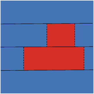
(a) Group-Cohort Pattern

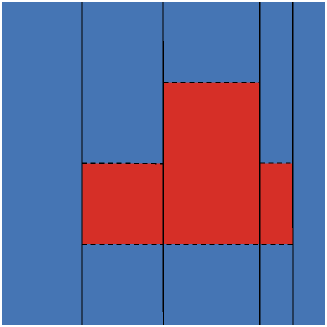
(b) Cohort-Group Pattern

Figure 2: Partitioned block structure on regression coefficients: firstly partition the blocks along the dash line and then along the dotted line.

We firstly introduce the group-cohort pattern in detail below. Let $K$ denote the split number of groups and $\mathcal{G}_{0k}$ denote the individual memberships for the $kth$ group for $k=1,\cdots,K$. Further, $R(k)$ denotes the number of blocks in the $kth$ group and $\mathcal{H}_{0r}(k)$ denote the temporal memberships for the $rth$ block in the $kth$ group $r=1,\cdots,R(k)$. Let $\boldsymbol{\Pi}$ denotes the grouped structure across individuals and $\widetilde{\Pi}=\{\pi_{ik},i=1,\cdots,N\}$ denotes an $N\times K$ matrix with $\pi_{ik}=1$ for $i\in\mathcal{G}_{0k}$ and $\pi_{ik}=0$ for $i\notin\mathcal{G}_{0k}$, indicating the group structure. Then, $\boldsymbol{\Pi}_{NTP\times KTP}=(\widetilde{\Pi}\otimes I_{T})\otimes I_{P}$. Furthermore, we let $\boldsymbol{W}$ denote the structural breaks in each group and for $k=1,\cdots,K,$ set $\widetilde{W}(k)=\{w_{tr}\}$ denote an $T\times R(k)$ matrix with $w_{tr}=1$ for $t\in\mathcal{H}_{0r}(k)$ and $w_{tr}=0$ for $r\notin\mathcal{H}_{0r}(k)$, which depicts the structural breaks under each group. Then, let $R=\sum_{k=1}^{K}R(k)$ and $\widetilde{\boldsymbol{W}}_{KT\times R}=\mathrm{diag}(\widetilde{W}(1),\cdots,\widetilde{W}(K))$ and $\boldsymbol{W}_{KTP\times RP}=\widetilde{\boldsymbol{W}}\otimes I_{P}$. As we can see, the number of blocks partitioned by group-cohort is not smaller than the number of real blocks, at least. Therefore, there is also a structural matrix to depict the relationship between group-cohort and real blocks. We use $\boldsymbol{Q}$ to depict the partitioned structure and $\boldsymbol{\eta}$ is the vector of values for split blocks with $L^{0}$ different values under the group-cohort pattern. It is obvious that some of the split blocks belong to same true block. Therefore, we set $\widetilde{\boldsymbol{Q}}_{R\times L^{0}}=\{q_{rl}\}$, with $r=\{1,\cdots,R\}$ and $l=\{1,\cdots,L^{0}\}$, denote an $R\times L^{0}$ matrix with $q_{rl}=1$ for $\eta_{r}=\alpha_{l}$, which depicts a structural matrix that integrate between spitted blocks and then $\boldsymbol{Q}_{RP\times L^{0}P}=\widetilde{\boldsymbol{Q}}\otimes I_{P}$. .As a result, $\boldsymbol{\beta}^{0}=\boldsymbol{\Pi}\boldsymbol{W}\boldsymbol{Q}\boldsymbol{\alpha}^{0}$ and the design matrix with known structural information $\mathbb{X}=\boldsymbol{X}\boldsymbol{\Pi}\boldsymbol{W}\boldsymbol{Q}$.

Similarly, we can also firstly set the cohorts structural matrix denoted by $\bar{\boldsymbol{W}}$ and then use $\bar{\boldsymbol{\Pi}}$ to describe the grouped structure in each cohorts in cohort-group pattern. Furthermore, $\bar{\boldsymbol{Q}}$ denotes the block integration in cohort-group pattern. Obviously, $\boldsymbol{\beta}^{0}=\Pi\boldsymbol{W}\boldsymbol{Q}\alpha^{0}=\bar{\boldsymbol{W}}\bar{\boldsymbol{\Pi}}\bar{\boldsymbol{Q}}\boldsymbol{\alpha^{0}}$, implying that we only need to select one of patterns. The two dimensional heterogeneous structure is more general than that in Okui and Wang (2020), due to the existence of structural matrices $\boldsymbol{Q}$ or $\bar{\boldsymbol{Q}}$, which depict the integration between splitted blocks and can be viewed as a mediator between different pattern.

To study the theoretical results of the proposed block regression estimator, we first investigate the asymptotic properties of the estimator with known block structure. Although, in practice, $L$ is generally unknown and such an estimator is infeasible. This infeasible procedure provides important information to which we should compare our feasible estimator. Let $\boldsymbol{\beta}^{0}$, $\boldsymbol{\alpha}^{0}$, $\mathcal{A}_{0}$ and $L_{0}$ denote the true values of $\boldsymbol{\beta}$, $\boldsymbol{\alpha}$, $\mathcal{A}$ and $L$, respectively. We also let $|\mathcal{A}_{l}|$ to signify the amount of elements in $\mathcal{A}_{l}$. $\mathcal{A}_{\min}=\min_{1\leq l\leq L}|\mathcal{A}_{l}|$ and $\mathcal{A}_{\max}=\max_{1\leq l\leq L}|\mathcal{A}_{l}|$, respectively represent the true minimum and maximum sample sizes among all blocks.

4.2 Asymptotic Property of the Infeasible Estimator with Known Two-Dimensional Heterogeneous Structure

If the underlying block structure $\mathcal{A}=\{\mathcal{A}_{l}:l=1,\cdots,L^{0}\}$ is known, which is equivalent to know the prior information of matrices $\boldsymbol{\Pi}$ and $\boldsymbol{W}$, $\boldsymbol{Q}$, and notice that $\boldsymbol{\beta}=\boldsymbol{\Pi}\boldsymbol{W}\boldsymbol{Q}\boldsymbol{\alpha}$, it is equivalent to consider $\widetilde{\boldsymbol{\alpha}}$ or $\widetilde{\boldsymbol{\beta}}=\boldsymbol{\Pi}\boldsymbol{W}\boldsymbol{Q}\widetilde{\boldsymbol{\alpha}}$. In this case, the post bi-integrative estimator is defined by:

$$\widetilde{\boldsymbol{\alpha}} = \mathop{{\rm argmin}}_{\boldsymbol{\alpha}\in\mathbb{R}^{PL}}\left\{\sum_{l=1}^{L}\sum_{(i,t)\in\mathcal{A}_{l}}(y_{it}-x_{it}^{\top}\boldsymbol{\alpha}_{l})^{2}\right\}$$ (18)

$$= \mathop{{\rm argmin}}_{\boldsymbol{\alpha}\in\mathbb{R}^{PL}}\left\{\|\boldsymbol{Y}-\mathbb{X}\boldsymbol{\alpha}\|^{2}\right\}$$

$$= \left(\mathbb{X}^{\top}\mathbb{X}\right)^{-1}\mathbb{X}^{\top}\boldsymbol{Y},$$

where $\widetilde{\boldsymbol{\alpha}}=(\widetilde{\alpha}_{1}^{\top},\cdots,\widetilde{\alpha}_{L^{0}}^{\top})^{\top}$.

Due to the block structure information, i.e., $\mathcal{A}$ is generally unknown in advance, the block-oracle estimators are infeasible in practice. However, it can shed light on the theoretical properties of the proposed estimators.

For investigating the statistical properties of the induced minimizer $\widetilde{\boldsymbol{\alpha}}$, we impose the following conditions,

• The noise vector $\boldsymbol{\epsilon}$ has sub-Gaussian tails such that $P(|\tau^{\top}\boldsymbol{\epsilon}|<\|\tau\|x)\geq 1-2\exp(-c_{1}x^{2})$ for any vector $\tau\in\mathbb{R}^{NT}$, $0<c_{1}<\infty$ and $x>0$, and $\epsilon_{it}$ is a sequence of independent random variables with $E(\epsilon_{it})=0$, $E(\epsilon_{it}^{2})=\sigma^{2}$ for $i=1,\cdots,N;t=1,\cdots,T$.

• (i) $\gamma_{\mathrm{min}}(\mathbb{X}^{\top}\mathbb{X})\geq c_{2}\mathcal{A}_{\mathrm{min}}$, $\gamma_{\mathrm{max}}(\mathbb{X}^{\top}\mathbb{X})\leq c_{3}NT.$ (ii) $\sum_{(i,t)\in\mathcal{A}_{l}}x_{it,p}^{2}=\left|\mathcal{A}_{l}\right|$, for $1\leq p\leq P$. (iii) $\sup_{it}\left\|\boldsymbol{x}_{it}\right\|\leq c_{4}\sqrt{P}$, (iv) $\left|\mathcal{A}_{\min}\right|\gg(L^{0}P)^{1/2}(NT)^{3/4}$, for some positive constants $c_{2}$, $c_{3}$ and $c_{4}$.

REMARK 1.

Condition (C1) about sub-Gaussian tails of the error is widely used in the literature of high-dimensional regressions. For Condition (C2), since

$$\mathbb{X}^{\top}\mathbb{X}=\mathrm{diag}(\sum_{(i,t)\in\mathcal{A}_{l}}x_{it}x_{it}^{\top},l=1,\cdots,L^{0}),$$

$\gamma_{\mathrm{min}}(\mathbb{X}^{\top}\mathbb{X})\geq\gamma_{\mathrm{min}}(\sum_{(i,t)\in\mathcal{A}_{l}}x_{it}x_{it}^{\top})\geq c_{2}\mathcal{A}_{\min}$, namely, the smallest eigenvalue of $\mathbb{X}^{\top}\mathbb{X}$ bounded by the smallest cardinal number of all blocks. Without loss of generality, we standardize the covariates in every sub-population, which is assumed in Condition (C2) (ii). Condition (C2) (iv) implies there should be enough observations within each block.

REMARK 2.

Usually, the proof of asymptotic normality on coefficients needs a little stronger assumption than consistency. For example, we only need finite second moment of $\epsilon_{it}$ to obtain consistency and finite fourth moment to obtain asymptotic normality. For simplicity, we are using the same assumptions for results (i) and (ii) in Theorem 1 below.

THEOREM 1.

(Asymptotic properties of the post bi-integrative estimator $\widetilde{\alpha}$)

• (Consistency and Rate of convergence) Under Conditions (C1) and (C2), we have

  $$\left\|\widetilde{\boldsymbol{\alpha}}-\boldsymbol{\alpha}^{0}\right\|\leq\Delta_{n}\text{,}\;\left\|\widetilde{\boldsymbol{\beta}}-\boldsymbol{\beta}^{0}\right\|\leq\sqrt{\left|\mathcal{A}_{\max}\right|}\Delta_{n}\text{, }\mathrm{and}\;\sup_{i,t}\left\|\widetilde{\boldsymbol{\beta}}_{it}-\boldsymbol{\beta}_{it}^{0}\right\|\leq\Delta_{n},$$

  where $\Delta_{n}=c_{1}^{-\frac{1}{2}}c_{2}^{-1}\sqrt{PL^{0}}\sqrt{NT\log(NT)}\left|\mathcal{A}_{\min}\right|^{-1}$.

• (Asymptotic normality) Under Conditions (C1) and (C2), we have

  $$s_{n}(\boldsymbol{d}_{n})^{-1}\boldsymbol{d}_{n}^{\top}(\widetilde{\boldsymbol{\alpha}}-\boldsymbol{\alpha}^{0})\overset{D}{\rightarrow}N(0,1),$$

  where

  $$s_{n}(\boldsymbol{d}_{n})=\sigma\{\boldsymbol{d}_{n}^{\top}(\mathbb{X}^{\top}\mathbb{X})^{-1}\boldsymbol{d}_{n}\}^{1/2},$$

  and $\sigma$ is the standard deviation for the error term, $\boldsymbol{d}_{n}$ is a $PL\times 1$ vector such that $\|\boldsymbol{d}_{n}\|=1$.

Theorem 1 states the post bi-integrative estimator $\widetilde{\boldsymbol{\alpha}}$ and the estimator $\widetilde{\boldsymbol{\beta}}$ with known block structure are consistent as both $N$ and $T$ $\rightarrow\infty$. Furthermore, the estimator $\widetilde{\boldsymbol{\beta}}$ is uniformly consistent across the samples.

4.3 Asymptotic Property of the Proposed Estimator with Unknown Block Structure

In practice, the block structure is unknown. In this section, we study the asymptotic properties of our proposed estimator with unknown block structure. We show that, under appropriate conditions, the induced local minimizer of the objective function (5) is asymptotically equivalent to the post bi-integrative estimator under a prior knowledge of block structure $\widetilde{\boldsymbol{\alpha}}$.

Let

$$b_{n}=\min_{\begin{subarray}{c}(i,t)\in\mathcal{A}_{l}\\ (j,t^{\prime})\in\mathcal{A}_{l^{\prime}}\end{subarray}}\left\|\boldsymbol{\beta}_{it}^{0}-\boldsymbol{\beta}_{jt^{\prime}}^{0}\right\|=\min_{l\neq l^{\prime}}\left\|\alpha_{l}^{0}-\alpha_{l^{\prime}}^{0}\right\|$$

be the minimum difference of the coefficients between any two blocks. In addition, we give assumption (C3):

• The scaled penalty functions $\rho_{\lambda}(s)=\lambda^{-1}\mathcal{P}_{\lambda}(s)$ and $\rho_{\gamma}(s)=\gamma^{-1}\mathcal{P}_{\gamma}(s)$ are symmetric, non-decreasing and concave on $[0,\infty)$. They are constant for $s\geq a\lambda$ or $s\geq a^{\prime}\gamma$ with some small constant $a>0$, $a^{\prime}>0$, and $\rho_{\lambda}(0)=\rho_{\gamma}(0)=0$. In addition, the first derivatives $\rho_{\lambda}^{\prime}(s)$ and $\rho_{\gamma}^{\prime}(s)$ exist and are continuous except for a finite number values for $s$ and $\rho_{\lambda}^{\prime}(0+)=\rho_{\gamma}^{\prime}(0+)=1$.

REMARK 3.

Condition (C3) is commonly given in the literature of concave penalties and penalized high-dimensional models such as , SCAD(Fan and Li, 2001) and MCP (Zhang, 2010). In addition, Lasso (Tibshirani et al., 2005) also satisfies (C1) and (C3) and just falls at the boundary of the class of penalty functions.

THEOREM 2.

Under Conditions (C1), (C2) and (C3) and $b_{n}>\max(a\lambda,a^{\prime}\gamma)$ with $\lambda\gg\Delta_{n}$ and $\gamma\gg\Delta_{n}$, the block-oracle estimator is a local minimizer of the objective function with probability tending to one, i.e., as both $N$ and $T$ $\rightarrow\infty$,

$$\boldsymbol{P}\left(\widehat{\boldsymbol{\beta}}(\lambda,\gamma)=\widetilde{\boldsymbol{\beta}}\right)\rightarrow 1,$$

where $\widehat{\boldsymbol{\beta}}(\lambda,\gamma)$ is the estimator by the integrative analysis.

The result in Theorem 2 implies that if the minimal difference of the coefficients between any two blocks is restricted by a lower bound, our proposed double penalized least square estimator can attain the block-oracle estimator and actually recover the true block structure with probability tending to one. Since the local minimizer $\widehat{\boldsymbol{\alpha}}$ of the objective function just attains the block-oracle estimator $\widetilde{\boldsymbol{\alpha}}$ , we can conclude the following corollary.

COROLLARY 1.

Let $\widehat{\boldsymbol{\alpha}}$ being the estimated coefficient vector of blocks, corresponding to $\widehat{\boldsymbol{\beta}}(\lambda,\gamma)$. Under conditions of Theorems 2, we obtain

$$s_{n}(\boldsymbol{d}_{n})^{-1}\boldsymbol{d}_{n}^{\top}(\widehat{\boldsymbol{\alpha}}-\boldsymbol{\alpha}^{0})\overset{D}{\rightarrow}N(0,1),$$

where

$$s_{n}(\boldsymbol{d}_{n})=\sigma\{\boldsymbol{d}_{n}^{\top}(\mathbb{X}^{\top}\mathbb{X})^{-1}\boldsymbol{d}_{n}\}^{1/2},$$

and $\sigma$ is the standard deviation for the error term, $\boldsymbol{d}_{n}$ is a $PL\times 1$ vector such that $\|\boldsymbol{d}_{n}\|=1$. In practice, the $\sigma$ is unknown in prior. The $\hat{\sigma}$ is estimated

$$\hat{\sigma}^{2}=\left(NT-\hat{L}P\right)^{-1}\sum_{i=1}^{N}\sum_{t=1}^{T}\left(y_{it}-\boldsymbol{x}_{it}^{\top}\hat{\boldsymbol{\beta}}_{it}\right)^{2},$$

with $\hat{\sigma}^{2}\overset{p}{\rightarrow}\sigma^{2}$.

The asymptotic distribution of the estimator provides a theoretical foundation for further statistical inference, such as the testing of heterogeneity. Next, we present an asymptotic $\chi^{2}$ test for hypothesis based on the estimators $\widehat{\boldsymbol{\alpha}}$. Specifically, we consider the null $H_{0}:\mathcal{B}\boldsymbol{\alpha}=0$ versus the alternative hypothesis $H_{1}:\mathcal{B}\boldsymbol{\alpha}\neq 0$, where $\mathcal{B}$ is a $q\times LP$ matrix and $q=$ rank$(\mathcal{B})$. Many important special cases belong to this hypothesis. For example, $H_{0lj}$: $\alpha_{lj}=0$, $l\in\{1,\ldots,L\}$ and $j\in\{1,\ldots,P\}$, which can be used to test the significance of the $j$th component of coefficients in the $l$th block; The null hypothesis $H_{0}:\alpha_{l}-\alpha_{l^{\prime}}=0$, $l,l^{\prime}\in\{1,\ldots,L\}$ can be used to test the existence of coefficients heterogeneity among blocks.

A standard $\chi^{2}$-test statistic for testing $H_{0}$: $\mathcal{B}\boldsymbol{\alpha}=0$ can be constructed as follows:

$$\mathcal{T}(\mathcal{B})=(\mathcal{B}\widehat{\boldsymbol{\alpha}})^{\top}(\mathcal{B}\widehat{\mathcal{V}}\mathcal{B}^{\top})^{-1}(\mathcal{B}\widehat{\boldsymbol{\alpha}}),$$ (19)

where $\widehat{\mathcal{V}}=\widehat{\sigma}^{2}(\mathbb{X}^{\top}\mathbb{X})^{-1}$.

THEOREM 3.

Under the null hypothesis and conditions in Theorem 2, $\mathcal{T}(\mathcal{B})\overset{D}{\rightarrow}\chi_{q}^{2}$, as both $N$ and $T\rightarrow\infty$.

Theorem 3 provides the asymptotic distribution of the test statistic $\mathcal{T}(\mathcal{B})$ under the null hypothesis $H_{0}$. Therefore, the $100(1-\tau)\%$ confidence interval for $\mathcal{B}\boldsymbol{\alpha}$ is given by

$$\mathbb{R}_{\tau}=\left\{\iota:(\mathcal{B}\widehat{\boldsymbol{\alpha}}-\iota)^{\top}(\mathcal{B}\widehat{\mathcal{V}}\mathcal{B}^{\top}-\iota)^{-1}(\mathcal{B}\widehat{\boldsymbol{\alpha}})\leq\chi_{q}^{2}(1-\tau)\right\},$$

where $\chi_{q}^{2}(1-\tau)$ is the $(1-\tau)$-quantile of the $\chi^{2}$ distribution with $q$ degrees of freedom.

5 Determination of the initial values and turning parameters

5.1 Initial values

The proposed ADMM algorithm requires an initialization. Initial value matters in accelerating the convergence of the iteration. In this paper, we propose the ridge fusion criterion to select initial parameters, since it has closed-form solution. Let

$$\ell_{R}(\boldsymbol{\beta})=\frac{1}{2}\sum_{i=1}^{N}\sum_{t=1}^{T}\left(y_{it}-\boldsymbol{x}_{it}^{\top}\boldsymbol{\beta}_{it}\right)^{2}+\frac{\lambda^{\ast}}{2}\sum_{i<j}\left\|\boldsymbol{\beta}_{i}-\boldsymbol{\beta}_{j}\right\|^{2}+\frac{\gamma^{\ast}}{2}\sum_{t<t^{\prime}}\left\|\boldsymbol{\beta}_{t}-\boldsymbol{\beta}_{t^{\prime}}\right\|^{2},$$ (20)

which can be written in matrix form

$$\ell_{R}(\boldsymbol{\beta})=\frac{1}{2}\left\|\boldsymbol{Y}-\boldsymbol{X}\boldsymbol{\beta}\right\|^{2}+\frac{\lambda^{\ast}}{2}\left\|\Omega\boldsymbol{\beta}\right\|^{2}+\frac{\gamma^{\ast}}{2}\left\|\Phi\boldsymbol{\beta}\right\|^{2},$$ (21)

where $\lambda^{\ast}$, $\gamma^{\ast}$ are the tuning parameters and chosen as $\lambda^{\ast}=\gamma^{\ast}=0.001$ in determination of initial values. By minimizing objective function (21), the initial value of $\boldsymbol{\beta}$ is given by

$$\boldsymbol{\beta}^{(1)}=\mathrm{vec}\left\{\{D^{\ast}(\widetilde{\boldsymbol{X}}\circ\boldsymbol{Y}-\widetilde{\boldsymbol{X}}\circ(M^{\ast}[\widetilde{\boldsymbol{X}}\circ(D^{\ast}(\widetilde{\boldsymbol{X}}\circ\boldsymbol{Y}))]^{+}))\}^{\top}\right\},$$

where

$$D^{\ast}=\left\{(\lambda^{\ast}N+\gamma^{\ast}T)\boldsymbol{I}_{NT}-\left[\psi(1_{N}1_{N}^{\top})\otimes\boldsymbol{I}_{T}+\phi\boldsymbol{I}_{N}\otimes(1_{T}1_{T}^{\top})\right]\right\}^{-1}$$

$$M^{\ast}=\left(I_{NT}+\left(\widetilde{\boldsymbol{X}}\widetilde{\boldsymbol{X}}^{\top}\right)\circ D^{\ast}\right)^{-1}.$$

5.2 Optimal tuning parameters

The proposed estimation is based on a penalized procedure that entails choices of tuning parameters $\lambda$ and $\gamma$.  Unsuitable choices of tuning parameters can produce poor estimates. Motivated by Wang et al. (2009); Ma and Huang (2016), we select the optimal tuning parameters $\widehat{\lambda}$ and $\widehat{\gamma}$ by minimizing the following modified BIC:

$$\mathrm{BIC}(\lambda,\gamma)=\log\left(\frac{1}{NT}\left\|\boldsymbol{Y}-\boldsymbol{X}\widehat{\boldsymbol{\beta}}(\lambda,\gamma)\right\|^{2}\right)+\mathcal{C}_{NT}\frac{\log(NT)}{NT}\left(\widehat{L}(\lambda,\gamma)P\right),$$ (22)

where $\mathcal{C}_{NT}$ is a constant or depending on $N$ and $T$. Following Ma and Huang (2016, 2017), we select $\mathcal{C}_{NT}=\log(NTP)$ in the Monte Carlo simulation and empirical analysis.

For convenience of analysis, we introduce some additional notations. Let $\mathcal{L}=\{1,2,\cdots,L_{\max}\}$, its three subsets $\mathcal{L}_{0}=\{L\in\mathcal{L}:L=L_{0}\}$, $\mathcal{L}_{\_{}}=\{L\in\mathcal{L}:L<L_{0}\}$, $\mathcal{L}_{+}=\{L\in\mathcal{L}:L>L_{0}\}$, represent cases of the true, under and over-fitting bi-integration, respectively. We establish asymptotic validity of the proposed BIC criterion in the following theorem.

THEOREM 4.

Supposing that all conditions of Theorem 2 hold, Then

$$p\left(\inf_{L\in\mathcal{L}_{\_{}}\cup\mathcal{L}_{+}}\mathrm{BIC}\left(L;\lambda,\gamma\right)>\mathrm{BIC}\left(L_{0};\lambda,\gamma\right)\right)\longrightarrow 1,\qquad\mathrm{as}\;(N,T)\longrightarrow\infty.$$ (23)

6 Monte Carlo simulation

In this section, we perform Monte Carlo simulation with $\mathcal{R}$ replications to investigate the finite-sample performance of the proposed bi-integration procedure with two data generating processes with various heterogeneous block structures on regression coefficients, measured by two aspects that one is the evaluation of the estimated regression coefficients and the other is the accuracy of bi-integration or recovery of block structures. We evaluate the performance of the estimated regression coefficients by root mean square error (RMSE) and its bias, measured by $\frac{1}{\mathcal{R}}\sum_{r=1}^{\mathcal{R}}\sqrt{\frac{1}{NTP}\|\widehat{\boldsymbol{\beta}}^{r}-\boldsymbol{\beta}^{0}\|^{2}}$ and $\frac{1}{\mathcal{R}}\sum_{r=1}^{\mathcal{R}}\left[\frac{1}{NTP}\sum_{i=1}^{N}\sum_{t=1}^{T}\sum_{j=1}^{P}(\widehat{\beta}_{itj}^{r}-\beta_{itj}^{0})\right]$ respectively, where $\widehat{\boldsymbol{\beta}}^{r}$ is the estimated coefficients vector in the $r$th replicate.

We evaluate the estimated numbers of blocks $\widehat{L}$ by the percentage (Per) of $\widehat{L}$ equal to the true number of blocks by the proposed BIGCORE procedure, calculated by $\frac{1}{\mathcal{R}}\sum_{r=1}^{\mathcal{R}}I(\widehat{L}^{r}=L^{0})$, where $\widehat{L}^{r}$ is the calculated number of blocks in the $r$th replicate. We also use the extended rand index(ERI), which measures percentage of correctly membership in each blocks. The Rand Index (RI) is used to evaluate the accuracy of clustering, which lies between 0 and 1, where higher values indicate better performance. Motivated by the formation of RI, we can get individual or period-specified RIs, denoted by $\text{RI}_{t}$ or $\text{RI}_{i}$ and define the ERI(T) and ERI(N) as the average of the whole periods and individuals respectively, i.e., ERI(T) $=\frac{1}{T}\sum_{t=1}^{T}\text{RI}_{t}$ and ERI(N)$=\frac{1}{N}\sum_{i=1}^{N}\text{RI}_{i}$. At last we adopt ERI=$\frac{1}{2}$[ERI(T)+ERI(N)] to evaluate the accuracy of BIGCORE procedure.

6.1 Data Generating Process

In this sections, we generate the simulated panel data observations $\{y_{it},x_{it}\}$, $i=1,\cdots,N$ and $t=1,\cdots,T$ by two data generating processes (DGP) with different block structures on regression coefficients and set the sample size as $N=20,40,60$ with $T=20,40,60$. In order to present the wide applicability of the proposed bi-integrating procedure, we consider the complex block structure in the example DGP1 and classical grouped structure in DGP2, respectively.

DGP1:(Block structure)

In this example, we generated observations from a two-dimensional heterogeneous panel data model,

$$y_{it}=\mu_{it}+x_{it}\eta_{it}+\epsilon_{it},\qquad i=1,\cdots,N;\quad t=1,\cdots,T.$$

Both the time-varying individual fixed effect $\mu_{it}$ and one-dimensional slope coefficient $\eta_{it}$ have the same structure of time-varying group memberships with common structural break depicted in Figure (1d). Then two blocks are considered and coefficient vector of the first block is set as $\boldsymbol{\alpha}_{1}=(-2,3)$ and let that of the second one be $\boldsymbol{\alpha}_{2}=(2,5)$ with the components corresponding to fixed effect $\mu_{it}$ and slope coefficient $\eta_{it}$, respectively. The block-based two-dimensional heterogeneous structure can be depicted by group-cohort pattern, such as, under the case of $N=40$, $T=40$, we consider group structure with $\mathcal{G}_{01}=\{1,\cdots,10,31,\cdots,40\}$, $\mathcal{G}_{02}=\{11,\cdots,20\}$, $\mathcal{G}_{03}=\{21,\cdots,30\}$ and the corresponding cohort structures under the assumed group formation are set by $\mathcal{H}_{01}(1)=\{1,\cdots,40\}$, $\mathcal{H}_{01}(2)=\{1,\cdots,19,30,\cdots,40\}$, $\mathcal{H}_{02}(2)=\{20,\cdots,29\}$, $\mathcal{H}_{01}(3)=\{1,\cdots,9,35,\cdots,40\}$, $\mathcal{H}_{02}(3)=\{10,\cdots,34\}$ and $\mathcal{H}_{01}(4)=\{1,\cdots,40\}$. Therefore, the ratio of number of block-specified observations is about $|\mathcal{A}_{1}|:|\mathcal{A}_{2}|\approx 3:1$. Other cases setting the sample sizes in the block structure under different combination of $N$ and $T$ has the similar way. The regressor $x_{it}$ is generated by

$$x_{it}=1+0.5\mu_{it}+\epsilon_{it},$$

where $\epsilon_{it}$ was taken from the standard normal distribution.

We consider the settings of homoscedasticity and heteroscedasticity on the error term by respectively generating $\epsilon_{it}\sim\ N(0,\sigma^{2})$ with $\sigma^{2}=0.5$, $\sigma^{2}=1$ and

$$\epsilon_{it}=\sigma_{it}e_{it},\sigma_{it}=\tau(0.05+0.05x_{it}^{2})^{1/2},$$

where $\tau=2$ or $\tau=1$ and $e_{it}\sim N(0,1)$.

DGP2(Grouped structure)

In this example, we consider the performance of proposed BIGCORE analysis in panel data model with grouped individual fixed effect and grouped slope coefficients. The Datasets are generated as:

$$y_{it}=\mu_{i}+x_{it}\eta_{i}+\epsilon_{it}.$$

Here, both the fixed effects and slope coefficients have identical grouped structure by randomly dividing the individuals into three groups with the proportion that $|\mathcal{G}_{1}|:|\mathcal{G}_{2}|:|\mathcal{G}_{3}|=3:3:4$, in which the true coefficients are $\boldsymbol{\alpha}_{1}=\{-2,3\}$, $\boldsymbol{\alpha}_{1}=\{2,6\}$ and $\boldsymbol{\alpha}_{3}=\{6,-1\}$, respectively. The regressor $x_{it}$ are generated as

$$x_{it}=1+0.5\mu_{i}+\epsilon_{it}.$$

Lastly, the error term is set as in DGP 1.

6.2 Simulation Results

In the simulation, we select the number of replicates $\mathcal{R}=100$. The grid of values of both tuning parameters $\lambda$ and $\gamma$ is set in the range of [0.1, 1.5] with step size 0.1. The fact that increasing grid of tuning parameters apparently improves integrative results is unconsidered here due to reducing computational cost. In order to accelerate the convergence of the proposed ADMM algorithm, we regard the converged value under the given combined tuning parameters as the initial value of the next iteration, instead of adopting identical initial values under different combined tuning parameters in the grid.

After one replicate, Figures (3) vividly presents the performance of our proposed BIGCORE analysis in estimating coefficients and block structure in DGP1 and DGP2 settings under $N=40$, $T=40$ and heteroscedasticity with $\tau=2$ and the figure elucidates that the developed method can achieve expected outcome because it can recover the true block or grouped structure correctly with consistent value of coefficient estimators. Another inevitable fact we should admit is that although Figures (3) actually shows ideal simulated results in one replicate, several worse BIGCORE results still occur occasionally, which is reflected by the misintegration that a little of observations may be wrongly partitioned, such as, it may occur in the replicates with the cases of large standard deviation of error term. Specifically, a little of observations originally belonging to red block are mistakenly bi-integrated into the blue block.

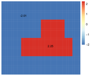
(a) Estimated fixed effect in DGP1

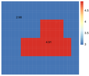
(b) Estimated slope efficient in DGP1

(c) Estimated fixed effect in DGP2

(d) Estimated slope efficient in DGP2

Figure 3: The estimates of result of fixed effect and slope efficient in DGP1 and DGP2 by one replicate.

For checking the representation of coefficients estimators, we report the RMSE and Bias of the slope coefficient for examples DGP1 and DGP2 in Tables (1) and Table (2), respectively, which elucidates that (i) both SCAD and MCP penalties present similar BIGCORE behaviors in terms of close values of RMSE and Bias, and both are also close to the oracle results, which is the reason we reject arguing the effective combination of the forms of double concave penalties; (ii) with increasing number of individuals or periods, the values of RMSE and the Bias decrease remarkably in all cases; (iii) the values of RMSE and Bias in DGP1 are relatively larger than that in DGP2. It may be owe to the more complex formation of block structure than that of grouped pattern and the group-specified cohort structure should be integrated in DGP1; (iv) the post estimators is recommended due to that it attains much smaller RMSE and Bias, especially as $N$ or $T$ increases. It is also noted that the estimation performance on slop coefficients under post-MCP is usually the same to that of post-SCAD, which is attributed to the common block structure recovery by both penalties.

For evaluating the accuracy of BIGCORE procedure in estimating the number of blocks, Table (3) and Table (4) reports the percentage of the estimated numbers of blocks equal to the true number of blocks by the SCAD and MCP shrinkage procedures under different cases of DGP1 and DGP2. In all cases, the percentage of correctly selecting the number of blocks increases as $N$ and $T$ are enlarged. The two concave penalties SCAD and MCP procedures have similar performance.

Another results under the evaluation criterion extended Rand index, which is used to measure the bi-integration ability of recovering the true underlying structures, are reported in Table (5), Table (6) and the results show that the extended Rand index are mostly close to one, which indicates the effectiveness of the proposed BIGCORE method. The results also imply that the BIGCORE performance was worsen with serious heteroscedasticity such as larger $\sigma^{2}$.

Table 1: The root mean square error (RMSE) and bias of the estimator of $\eta_{it}$ in DGP1

		Homoscedasticity				Heteroscedasticity
		$\sigma^{2}=0.5$		$\sigma^{2}=1$		$\tau=1$		$\tau=2$
(N,T)	Methods	RMSE	Bias	RMSE	Bias	RMSE	Bias	RMSE	Bias
(20, 20)	SCAD	0.0718	-0.0005	0.1442	0.0094	0.0645	-0.0066	0.3288	0.0286
	Post-SCAD	0.0517	0.0002	0.0842	0.0165	0.0529	0.0005	0.1616	0.0070
	MCP	0.0713	-0.001	0.1431	0.0159	0.0656	-0.0052	0.3258	0.0245
	Post-MCP	0.1122	0.0001	0.0894	0.0189	0.0529	-0.0009	0.1644	0.0071
	Oracle	0.0440	0.0002	0.0587	0.0122	0.0491	-0.0009	0.1473	0.0085
(40, 20)	SCAD	0.0596	-0.0033	0.1576	0.0126	0.0531	-0.0033	0.3984	0.0312
	Post-SCAD	0.0354	0.0015	0.0716	0.0082	0.0336	0.0026	0.2259	0.0034
	MCP	0.0585	-0.0037	0.1558	0.0149	0.0558	-0.0033	0.3903	0.0309
	Post-MCP	0.0354	0.00015	0.0725	0.0087	0.0379	0.0023	0.2216	0.0031
	Oracle	0.0300	0.0007	0.0443	0.0037	0.0324	0.0021	0.2048	0.0041
(20, 40)	SCAD	0.0728	-0.0039	0.1429	0.0057	0.0608	-0.0055	0.2622	0.1058
	Post-SCAD	0.0344	0.0002	0.0458	0.0029	0.0429	-0.0044	0.1360	0.0195
	MCP	0.0732	-0.0016	0.1426	0.0064	0.0623	-0.0048	0.2576	0.0999
	Post-MCP	0.0345	0.0002	0.0463	0.0027	0.0411	-0.0037	0.1301	0.0046
	Oracle	0.0331	0.0002	0.0415	0.0029	0.0382	-0.0038	0.0727	0.0016
(40, 40)	SCAD	0.0541	-0.0058	0.1315	0.0030	0.0414	-0.0057	0.1238	0.0319
	Post-SCAD	0.0226	-0.0026	0.0306	0.0002	0.0226	0.0013	0.0491	0.0016
	MCP	0.1179	-0.0075	0.1306	0.0035	0.0489	-0.0029	0.1217	0.0341
	Post-MCP	0.0226	-0.0027	0.0301	0.0002	0.0263	0.0018	0.0473	0.0022
	Oracle	0.0226	-0.0026	0.0298	0.0001	0.0226	0.0013	0.0470	0.0014
(60, 40)	SCAD	0.0569	-0.0037	0.1336	0.0034	0.0447	-0.0037	0.1748	0.0844
	Post-SCAD	0.0184	0.0012	0.0278	-0.0015	0.0203	0.0014	0.0496	0.0016
	MCP	0.0561	-0.0030	0.1332	0.0041	0.0448	-0.0037	0.0415	0.0013
	Post-MCP	0.0186	0.0012	0.0253	-0.0018	0.0202	0.00014	0.0481	0.0015
	Oracle	0.0184	0.0012	0.0260	-0.0017	0.0203	-0.0009	0.0382	-0.0013
(40, 60)	SCAD	0.0549	-0.0066	0.1294	0.0030	0.0406	-0.0025	0.1701	0.0805
	Post-SCAD	0.0197	0.0008	0.0295	0.0004	0.0190	-0.0009	0.0699	0.0027
	MCP	0.0544	-0.0062	0.2676	-0.0015	0.0407	-0.0027	0.1702	0.0110
	Post-MCP	0.0197	0.0008	0.0298	0.0004	0.0190	-0.0009	0.0624	0.0013
	Oracle	0.0197	0.0008	0.0257	0.0004	0.0190	-0.0009	0.0482	-0.0013
(60, 60)	SCAD	0.0455	-0.0013	0.1158	-0.0024	0.0385	-0.0019	0.1178	0.0156
	Post-SCAD	0.0197	0.0063	0.0284	0.0019	0.0188	-0.0007	0.0485	-0.0012
	MCP	0.0827	-0.0011	0.1212	-0.0031	0.0382	-0.0019	0.1193	0.0163
	Post-MCP	0.0197	0.0063	0.0285	0.0019	0.0188	-0.0007	0.0488	-0.0014
	Oracle	0.0197	0.0063	0.0284	0.0019	0.0188	-0.0007	0.0281	0.0041

Table 2: The root mean square error (RMSE) and bias of the estimator of $\eta_{i}$ in DGP2.

		Homoscedasticity				Heteroscedasticity
		$\sigma^{2}=0.5$		$\sigma^{2}=1$		$\tau=1$		$\tau=2$
(N,T)	Methods	RMSE	Bias	RMSE	Bias	RMSE	Bias	RMSE	Bias
(20,20)	SCAD	0.0924	0.0031	0.2424	0.0183	0.1030	0.0051	0.3288	0.0286
	Post-SCAD	0.0480	-0.0036	0.0881	-0.0142	0.0666	-0.0041	0.1615	0.0069
	MCP	0.0924	0.0036	0.2428	0.0187	0.1046	0.0051	0.2129	-0.0189
	Post-MCP	0.0474	-0.0036	0.0867	-0.0132	0.0666	-0.0042	0.0812	-0.0018
	Oracle	0.0457	-0.0037	0.0655	-0.0109	0.0666	-0.0041	0.1473	0.0085
(40, 20)	SCAD	0.0978	0.0039	0.2443	-0.0153	0.0998	-0.0054	0.3102	-0.0231
	Post-SCAD	0.0759	0.0011	0.0754	0.0172	0.0674	0.0042	0.1561	0.0054
	MCP	0.0962	0.0034	0.2453	-0.0153	0.1009	-0.0059	0.3154	-0.0231
	Post-MCP	0.0714	0.0037	0.0763	0.0172	0.0647	0.0045	0.1567	0.0058
	Oracle	0.0314	0.0038	0.0639	0.0111	0.0638	-0.0019	0.1248	0.0041
(20, 40)	SCAD	0.0344	0.0025	0.0773	0.0055	0.0509	0.0025	0.0966	0.0042
	Post-SCAD	0.0315	-0.0014	0.0483	-0.0121	0.0507	0.0008	0.0954	-0.0079
	MCP	0.0345	0.0023	0.1811	0.0051	0.0513	0.0028	0.0972	0.0042
	Post-MCP	0.0315	-0.0012	0.1392	-0.0121	0.0492	0.0008	0.0955	-0.0079
	Oracle	0.0315	-0.0014	0.0483	-0.0121	0.0507	0.0008	0.0954	-0.0079
(40,40)	SCAD	0.0646	0.0034	0.1635	0.0064	0.0688	0.0046	0.2869	0.0595
	Post-SCAD	0.0209	-0.0002	0.0317	-0.0002	0.0346	0.0025	0.0932	0.0019
	MCP	0.0646	0.0036	0.1628	0.0064	0.0686	0.0040	0.2828	0.0560
	Post-MCP	0.0208	-0.0003	0.0317	-0.0002	0.0344	0.0027	0.0936	0.0020
	Oracle	0.0209	-0.0002	0.0317	-0.0002	0.0346	0.0025	0.0707	0.0016
(60, 40)	SCAD	0.0998	0.0084	0.2182	0.0210	0.0924	0.0054	0.2414	-0.0247
	Post-SCAD	0.0189	0.0014	0.0279	-0.0015	0.0189	-0.0009	0.0248	0.0041
	MCP	0.0977	0.0081	0.2179	0.0100	0.0934	0.0058	0.2399	-0.0247
	Post-MCP	0.0169	0.0014	0.0279	-0.0015	0.0189	-0.0009	0.0249	0.0041
	Oracle	0.0189	0.0014	0.0278	-0.0015	0.0188	-0.0009	0.0167	0.0041
(40, 60)	SCAD	0.0352	0.0021	0.0545	0.0025	0.0354	0.0015	0.0828	0.0047
	Post-SCAD	0.0189	-0.0001	0.0334	-0.0001	0.0132	0.0017	0.0827	0.0010
	SCAD	0.0349	0.0020	0.0542	0.0023	0.0348	0.0019	0.0833	0.0049
	Post-SCAD	0.0188	-0.0001	0.0329	-0.0001	0.0132	0.0017	0.0845	0.0011
	Oracle	0.0188	-0.0001	0.0276	-0.0001	0.0132	0.0017	0.0845	0.0009
(60, 60)	SCAD	0.0443	0.0029	0.1153	0.0055	0.0414	0.0037	0.2469	0.0315
	Post-SCAD	0.0189	-0.0001	0.0299	-0.0002	0.0162	0.0021	0.0724	0.0011
	MCP	0.0438	0.0030	0.1152	0.0054	0.0414	0.0037	0.2421	0.0315
	Post-MCP	0.0189	-0.0001	0.0294	-0.0002	0.0162	0.0021	0.0724	0.0017
	Oracle	0.0189	-0.0001	0.0217	-0.0002	0.0162	0.0027	0.0619	0.0009

Table 3: The percentage(Per) of $\widehat{L}$ equal to the true number of blocks in DGP1.

		Homoscedasticity			Heteroscedasticity
		$\sigma^{2}=0.5$	$\sigma^{2}=1$		$\tau=1$	$\tau=2$
(N,T)	Methods	Per	Per		Per	Per
(20, 20)	SCAD	0.99	0.89		1.00	0.80
	MCP	0.99	0.89		1.00	0.81
(40, 20)	SCAD	1.00	0.90		0.97	0.84
	MCP	1.00	0.90		0.97	0.84
(20, 40)	SCAD	0.99	0.85		0.97	0.89
	MCP	0.99	0.87		0.97	0.88
(40, 40)	SCAD	0.98	0.89		1.00	0.92
	MCP	0.98	0.89		1.00	0.92
(60, 40)	SCAD	0.98	0.93		0.99	0.94
	MCP	0.98	0.93		0.98	0.93
(40, 60)	SCAD	1.00	0.91		0.99	0.91
	MCP	1.00	0.92		0.99	0.92
(60, 60)	SCAD	1.00	0.95		0.99	0.94
	MCP	1.00	0.95		0.99	0.94

Table 4: The percentage(Per) of $\widehat{L}$ equal to the true number of blocks in DGP2.

		Homoscedasticity			Heteroscedasticity
		$\sigma^{2}=0.5$	$\sigma^{2}=1$		$\tau=1$	$\tau=2$
(N,T)	Methods	Per	Per		Per	Per
(20, 20)	SCAD	1.00	1.00		1.00	0.99
	MCP	1.00	1.00		1.00	1.00
(40, 20)	SCAD	1.00	1.00		1.00	0.98
	MCP	1.00	1.00		1.00	1.00
(20, 40)	SCAD	1.00	1.00		1.00	1.00
	MCP	1.00	1.00		1.00	1.00
(40, 40)	SCAD	1.00	1.00		1.00	0.97
	MCP	1.00	1.00		1.00	0.98
(60, 40)	SCAD	1.00	1.00		1.00	1.00
	MCP	1.00	1.00		1.00	1.00
(40, 60)	SCAD	1.00	1.00		1.00	1.00
	MCP	1.00	1.00		1.00	1.00
(60, 60)	SCAD	1.00	1.00		1.00	1.00
	MCP	1.00	1.00		1.00	1.00

Table 5: The values of Extended Rand Index (ERI) in DGP1

		Homoscedasticity		Heteroscedasticity
		$\sigma^{2}=0.5$	$\sigma^{2}=1$	$\tau=1$	$\tau=2$
(N,T)	Methods	ERI	ERI	ERI	ERI
(20, 20)	SCAD	0.9974	0.9892	0.9991	0.9880
	MCP	0.9973	0.9897	0.9994	0.9884
(40, 20)	SCAD	0.9978	0.9863	0.9983	0.9742
	MCP	0.9978	0.9854	0.9982	0.9731
(20, 40)	SCAD	0.9968	0.9879	0.9981	0.9801
	MCP	0.9969	0.9878	0.9979	0.9995
(40, 40)	SCAD	0.9982	0.9902	0.9990	0.9926
	MCP	0.9982	0.9898	0.9990	0.9926
(60, 40)	SCAD	0.9980	0.9899	0.9989	0.9954
	MCP	0.9979	0.9893	0.9989	0.9956
(40, 60)	SCAD	0.9981	0.9903	0.9990	0.9949
	MCP	0.9980	0.9900	0.9990	0.9953
(60, 60)	SCAD	0.9981	0.9903	0.9990	0.9949
	MCP	0.9980	0.9900	0.9990	0.9953

Table 6: The values of Extended Rand Index(ERI) in DGP2.

		Homoscedasticity		Heteroscedasticity
		$\sigma^{2}=0.5$	$\sigma^{2}=1$	$\tau=1$	$\tau=2$
(N,T)	Methods	ERI	ERI	ERI	ERI
(20, 20)	SCAD	0.9986	0.9932	0.9993	0.9894
	MCP	0.9986	0.8910	0.9993	0.9142
(40, 20)	SCAD	0.9647	0.9274	0.9814	0.9415
	MCP	0.9659	0.9243	0.9820	0.9409
(20, 40)	SCAD	0.9999	0.9989	1.0000	0.9995
	MCP	0.9999	0.9981	0.9998	0.9986
(40, 40)	SCAD	0.9992	0.9963	0.9996	0.9894
	MCP	0.9993	0.9965	0.9996	0.9142
(60, 40)	SCAD	0.9816	0.9428	0.9883	0.9512
	MCP	0.9799	0.9449	0.9901	0.9564
(40, 60)	SCAD	0.9999	0.9992	1.0000	0.9894
	MCP	0.9999	0.9990	1.0000	0.9887
(60, 60)	SCAD	0.9996	0.9982	0.9998	0.9901
	MCP	0.9996	0.9979	0.9998	0.9912

7 Empirical application

In this section, we apply the proposed BIGCORE procedure to measure the heterogeneous impact of inputs on the economic output. Based on the classical Solow model about economic growth equation, the economic output is mainly determined by technological progress, Capital and Labor, and we establish the following regression given by

$$\log(\mathrm{GDP}_{it})=\mu_{it}+\beta_{1,it}\log(\mathrm{Hc}_{it})+\beta_{2,it}\log(\mathrm{Ck}_{it})+\beta_{3,it}\log(\mathrm{Ngd}_{it})+\epsilon_{it},$$ (24)

where $\mathrm{GDP}_{it}$ denotes the real gross domestic product, technological progress are usually represented by human capital(Hc) in the empirical literature, Ck is physical capital stock and Ngd denotes population growth plus break even investments of $5\%$. The coefficients represent different economic meanings, such as, the slope coefficient $\beta_{2,it}$ is the elasticity of investment on output. In the whole world, countries with different resource endowments and technical power are at different stages of development. For the developing countries, the elasticity of investment on output is larger than that of developed countries according to the law of economic development. From the perspective of period, the improvement of technological progress on economic development is diminishing marginally or remain stable, and the marginal effect shifts to higher level as the emergence of new technologies. Therefore, the slope coefficients are heterogeneous across countries and may exist structural breaks in the long span.

The original data are available form the Penn World Tables 8 and can be directly obtained from the package xtdcce2 of Stata. The dataset contains panel data with 92 countries and its yearly observations from 1963 until 2007. Same as Qian and Su (2016), the observations are averaged by each 5 years. Thus, we finally get panel data with $N=92$, $T=9$ and $P=4$. In addition, we set a grid of turning parameters $\lambda$ and $\gamma$ from 0.2 to 3 with interval of 0.2. Finally, we get two blocks $\hat{L}=2$ shown in Figure (4) that the blue block is denoted by $\mathcal{A}_{1}$ and the red block is denoted by $\mathcal{A}_{2}$. In the estimation process, optimal $\lambda$ and $\gamma$ are selected by 2.6 and 1.6 respectively, according to the modified BIC. The penalized estimators and post estimators based on the estimated block structure are reported in the Table (7) and the results imply that all the penalized estimators are statistically significant and most post estimators are statistically significant, except for $\beta_{2,it}$ and $\beta_{3,it}$ in block $\mathcal{A}_{2}$. What’s more, the standard errors of post estimators are smaller than that of penalized estimators, which is consistent to that of the Monte Carlo simulation. In conclusion, the block heterogeneity is remarkable in Solow model based on the BIGCORE method that the elasticity or marginal coefficient are significant across blocks, owing to different endowments across countries, continuous development and progress.

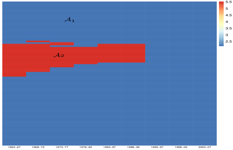
Figure 4: The estimated block structure and the corresponded estimation of intercept.

Table 7: Empirical Results.

	Dependent Variable: $\log({\rm GDP})$
	Penalized Estimators		Post Estimators
	$\hat{\mathcal{A}}_{1}$	$\hat{\mathcal{A}}_{2}$	$\hat{\mathcal{A}}_{1}$	$\hat{\mathcal{A}}_{2}$
Intercept	$2.144{{*}{*}{*}}$	$5.521{{*}{*}{*}}$	$1.719{{*}{*}{*}}$	$5.540{{*}{*}{*}}$
	$(0.708)$	$(1.978)$	$(0.514)$	$(1.436)$
$\log$(Hc)	$2.525{{*}{*}{*}}$	$1.336{{*}{*}{*}}$	$2.221{{*}{*}{*}}$	$2.735{{*}{*}{*}}$
	$(0.165)$	$(0.429)$	$(0.120)$	$(0.312)$
$\log$(Ck)	$0.184{{*}{*}{*}}$	$3.005{{*}{*}{*}}$	$0.127{{*}{*}{*}}$	$-0.010$
	$(0.021)$	$(0.163)$	$(0.016)$	$(0.119)$
$\log$(Ngd)	$-0.898{{*}{*}{*}}$	$-9.645{{*}{*}{*}}$	$-1.389{{*}{*}{*}}$	$-0.321$
	$(0.306)$	$(0.836)$	$(0.222)$	$(0.607)$
Obs(df = 820)	828	828	828	828
Std. Error	0.924	0.924	0.671	0.671
Note:	∗p$<$0.1; ∗∗p$<$0.05; ∗∗∗p$<$0.01
	Standard error are in parentheses

8 Conclusion

In this work, we consider a general panel data model with two-dimensional heterogeneous coefficients and propose a novel BIGCORE procedure to discover the assumed block structure and obtain the estimators simultaneously. An ADMM algorithm is developed to iteratively solve the objective function with double concave fused penalties. Simulated studies suggest that our method is effective and show fine performance in conducting BIGCORE analysis by correctly estimating the structure and coefficients. A modified Bayesian information criteria is proposed to get rid of the knotty issue that the double tuning parameters are sensitive to the estimators. However, computational complexity is growing with the increasing number of samples and time periods, causing the burden of the ADMM algorithm. What’s more, this work assumes that all coefficients have identical block structure under two-dimensional heterogeneity, which motivates us to plan to extend the BIGCORE analysis to the case of covariate-specified block structure. All or other issues, including the consideration of two-dimensional heterogeneous panel model with interactive effects, are worthy to be studied in the further research.

Proof of Theorem 1

The post bi-integrative estimator defined in (18) has expression given by

$$\widetilde{\boldsymbol{\alpha}}=(\mathbb{X}^{\top}\mathbb{X})^{-1}\mathbb{X}^{\top}\boldsymbol{Y},$$

and

$$\widetilde{\boldsymbol{\alpha}}-\boldsymbol{\alpha}^{0}=(\mathbb{X}^{\top}\mathbb{X})^{-1}\mathbb{X}^{\top}\boldsymbol{\epsilon},$$

Hence

$$\left\|\widetilde{\boldsymbol{\alpha}}-\boldsymbol{\alpha}^{0}\right\|\leq\|(\mathbb{X}^{\top}\mathbb{X})^{-1}\|\|\mathbb{X}^{\top}\boldsymbol{\epsilon}\|.$$

Condition (C2) (i) implies that

$$\|(\mathbb{X}^{\top}\mathbb{X})^{-1}\|\leq c_{2}^{-1}(\mathcal{A}_{\min})^{-1}.$$

Moreover, $\boldsymbol{X}\Pi\boldsymbol{W}\boldsymbol{Q}=\left[x_{it}^{\top}\boldsymbol{1}_{\left\{(i,t)\in\mathcal{A}_{l}\right\}}\right]_{i=1,t=1,l=1}^{N,T,L}$, $\sum_{i=1}^{N}\sum_{t=1}^{T}x_{it}^{2}\boldsymbol{1}_{\left\{(i,t)\in\mathcal{A}_{l}\right\}}=\left|\mathcal{A}_{l}\right|,$

$$\left\|(\boldsymbol{X}\Pi\boldsymbol{W}\boldsymbol{Q})^{\top}\boldsymbol{\epsilon}\right\|_{\infty}=\sup_{p,l}\Big{|}\sum_{i=1}^{N}\sum_{t=1}^{T}x_{itp}\epsilon_{it}\boldsymbol{1}_{\left\{(i,t)\in\mathcal{A}_{l}\right\}}\Big{|},$$

$$P\left(\|\mathbb{X}^{\top}\boldsymbol{\epsilon}\|_{\infty}>C\sqrt{NT\log(NT)}\right)=P\left(\|(\boldsymbol{X}\Pi\boldsymbol{W}\boldsymbol{Q})^{\top}\boldsymbol{\epsilon}\|_{\infty}>C\sqrt{NT\log(NT)}\right).$$

For some constant $0<C<\infty$, by union bound, we have

$$P\left(\|(\boldsymbol{X}\Pi\boldsymbol{W}\boldsymbol{Q})^{\top}\boldsymbol{\epsilon}\|_{\infty}>C\sqrt{NT\log(NT)}\right)$$

$$\leq \sum_{p=1,l=1}^{P,L}P\left(\Big{|}\sum_{n=1}^{N}\sum_{t=1}^{T}x_{itp}\boldsymbol{1}_{\{(i,t)\in\mathcal{A}_{l}\}}\epsilon_{it}\Big{|}>C\sqrt{NT\log(NT)}\right)$$

$$\leq \sum_{p=1,l=1}^{P,L}P\left(\Big{|}\sum_{i=1}^{N}\sum_{t=1}^{T}x_{itp}\boldsymbol{1}_{\{(i,t)\in\mathcal{A}_{l}\}}\epsilon_{it}\Big{|}>C\sqrt{|\mathcal{A}_{l}|\log(NT)}\right)$$

$$\leq 2\sum_{p=1,l=1}^{P,L}\exp\left(-c_{1}C^{2}\log(NT)\right)$$

$$= 2PL(NT)^{-c_{1}C^{2}}.$$

Since $\|\mathbb{X}^{\top}\boldsymbol{\epsilon}\|\leq\sqrt{LP}\|\mathbb{X}^{\top}\boldsymbol{\epsilon}\|_{\infty},$ then

$$P\left(\|\mathbb{X}^{\top}\boldsymbol{\epsilon}\|>C\sqrt{PL}\sqrt{NT\log(NT)}\right)\leq 2PL(NT)^{-c_{1}C^{2}}.$$

Therefore, we have with probability at least $1-2PL(NT)^{-c_{1}C^{2}}$,

$$\left\|\boldsymbol{\widetilde{\alpha}}-\boldsymbol{\alpha}^{0}\right\|\leq Cc_{2}^{-1}\sqrt{PL}\sqrt{NT\log(NT)}\left|\mathcal{A}_{\min}\right|^{-1}.$$

Therefore, we need $\left|\mathcal{A}_{\min}\right|\gg(LP)^{1/2}(NT)^{3/4}$, and the result of consistency in Theorem 1 (i) is proved by letting $C=c_{1}^{-1/2}$,

$$\left\|\tilde{\beta}-\boldsymbol{\beta}^{0}\right\|^{2} =\sum_{l=1}^{L}\sum_{(i,t)\in\mathcal{A}_{l}}\left\|\widetilde{\boldsymbol{\alpha}}-\boldsymbol{\alpha}^{0}\right\|^{2}\leq\left|\mathcal{A}_{\max}\right|\sum_{l=1}^{L}\left\|\widetilde{\boldsymbol{\alpha}}-\boldsymbol{\alpha}^{0}\right\|^{2}$$

$$=\left|\mathcal{A}_{\max}\right|\left\|\widetilde{\boldsymbol{\alpha}}-\boldsymbol{\alpha}^{0}\right\|^{2}\leq\left|\mathcal{A}_{\max}\right|\Delta_{n}^{2},$$

$$\sup_{i,t}\left\|\tilde{\beta}_{it}-\boldsymbol{\beta}_{it}^{0}\right\|=\sup_{l}\left\|\widetilde{\boldsymbol{\alpha}}-\boldsymbol{\alpha}_{l}^{0}\right\|\leq\left\|\widetilde{\boldsymbol{\alpha}}-\boldsymbol{\alpha}^{0}\right\|\leq\Delta_{n}.$$

For any $\boldsymbol{d}_{n}\in\mathbb{R}^{LP}$ with $\|\boldsymbol{d}_{n}\|=1$ and $\mathbb{X}=(\mathbb{X}_{1\cdot},\cdots,\mathbb{X}_{(NT)\cdot})^{\top}$

$$\boldsymbol{d}_{n}^{\top}(\widetilde{\boldsymbol{\alpha}}-\boldsymbol{\alpha}^{0})=\sum_{i=1}^{N}\sum_{t=1}^{T}\boldsymbol{d}_{n}^{\top}(\mathbb{X}^{\top}\mathbb{X})^{-1}\mathbb{X}_{(it)\cdot}\epsilon_{it}.$$

Hence, $E\{\boldsymbol{d}_{n}^{\top}(\widetilde{\boldsymbol{\alpha}}-\boldsymbol{\alpha}^{0})\}=0$

$$var\{\boldsymbol{d}_{n}^{\top}(\widetilde{\boldsymbol{\alpha}}-\boldsymbol{\alpha}^{0})\}=s_{n}(\boldsymbol{d}_{n})^{2}=\sigma^{2}\boldsymbol{d}_{n}^{\top}(\mathbb{X}^{\top}\mathbb{X})^{-1}\boldsymbol{d}_{n}\geq\sigma^{2}c_{3}^{-1}(NT)^{-1}.$$

Moreover, for any $\epsilon>0$,

$$\sum_{i=1}^{N}\sum_{t=1}^{T}E\Big{\{}\left(\boldsymbol{d}_{n}^{\top}(\mathbb{X}^{\top}\mathbb{X})^{-1}\mathbb{X}_{(it)\cdot}\epsilon_{it}\right)^{2}\boldsymbol{1}_{\{|\boldsymbol{d}_{n}^{\top}(\mathbb{X}^{\top}\mathbb{X})^{-1}\mathbb{X}_{(it)\cdot}\epsilon_{it}|>\epsilon s_{n}(\boldsymbol{d}_{n})\}}\Big{\}}$$

$$\leq NT\Big{\{}E\left(\boldsymbol{d}_{n}^{\top}(\mathbb{X}^{\top}\mathbb{X})^{-1}\mathbb{X}_{(it)\cdot}\epsilon_{it}\right)^{4}\Big{\}}^{1/2}\Big{\{}P\{|\boldsymbol{d}_{n}^{\top}(\mathbb{X}^{\top}\mathbb{X})^{-1}\mathbb{X}_{(it)\cdot}\epsilon_{it}|>\epsilon s_{n}(\boldsymbol{d}_{n})\}\Big{\}}^{1/2}.$$

Since $E(\epsilon_{it}^{4})\leq c$ by Condition (C1) and $\sup_{it}\|x_{it}\|\leq c_{4}\sqrt{P}$ by Condition (C3), then

$$\{E(\boldsymbol{d}_{n}^{\top}(\mathbb{X}^{\top}\mathbb{X})^{-1}\mathbb{X}_{(it)\cdot}\epsilon_{it})^{4}\}^{1/2}\leq\|\boldsymbol{d}_{n}^{\top}(\mathbb{X}^{\top}\mathbb{X})^{-1}\|^{2}\|\mathbb{X}_{it}\|^{2}[E(\epsilon_{it}^{4})]^{1/2}\leq c^{\prime}c_{2}^{-2}c_{4}^{2}|\mathcal{A}_{min}|^{-2}LP$$

, for some constant $0<c^{\prime}<\infty$.

Similarly, $E\left(\boldsymbol{d}_{n}^{\top}(\mathbb{X}^{\top}\mathbb{X})^{-1}\mathbb{X}_{(it)\cdot}\epsilon_{it}\right)^{2}\leq c^{\prime\prime}c_{2}^{-2}c_{4}^{2}|\mathcal{A}_{min}|^{-2}LP$, for some constant $0<c^{\prime\prime}<\infty$. Thus

$$P\Big{\{}|\boldsymbol{d}_{n}^{\top}(\mathbb{X}^{\top}\mathbb{X})^{-1}\mathbb{X}_{i}^{\top}\epsilon_{i}|>\epsilon s_{n}(\boldsymbol{d}_{n})\Big{\}} \leq E\left(\boldsymbol{d}_{n}^{\top}(\mathbb{X}^{\top}\mathbb{X})^{-1}\mathbb{X}_{it}\epsilon_{it}\right)^{2}/\{\epsilon^{2}s_{n}(\boldsymbol{d}_{n})^{2}\}$$

$$\leq c^{\prime\prime}c_{2}^{-2}c_{4}^{2}c_{3}^{-1}\sigma^{-2}\epsilon^{-2}\left|\mathcal{A}_{\min}\right|^{-2}LPNT,$$

for some constant $c^{\prime}$. Therefore, by the above results, we have

$$s_{n}(\boldsymbol{d}_{n})^{-2}\sum_{i=1}^{N}\sum_{t=1}^{T}E\Big{\{}\left(\boldsymbol{d}^{\top}(\mathbb{X}^{\top}\mathbb{X})^{-1}\mathbb{X}_{(it)\cdot}\epsilon_{it}\right)^{2}\boldsymbol{1}_{\{|\boldsymbol{d}^{\top}(\mathbb{X}^{\top}\mathbb{X})^{-1}\mathbb{X}_{(it)\cdot}\epsilon_{it}|>\epsilon s_{n}(\boldsymbol{d})\}}\Big{\}}$$

$$\leq O\left\{(NT)^{3}\left|\mathcal{A}_{\min}\right|^{-4}(LP)^{2}\right\}=o(1).$$

The last equality follows from the assumption that $\left|\mathcal{A}_{\min}\right|\gg(LP)^{1/2}(NT)^{3/4}$. Then, the result in this Theorem follows from Lindeberg-Feller Central Limit Theorem.

Proof of Theorem 2

In order to prove of Theorem 2, we firstly split the true block structure of coefficients as shown in Figure 5, which is different from the pattern of group-cohort or cohort-group in Figure 2. In this pattern, we firstly split the sample according to individuals as the true group structure and then split the sample across the temporal dimension. The difference lies how the cohorts are split. If there exist structural breaks for any individuals at given time period, we split the cohorts for all individuals, instead of splitting the cohorts under given groups. As we can see, the number of split blocks is larger. Let,

$$L(\boldsymbol{\beta})=\frac{1}{2}\|\boldsymbol{Y}-\boldsymbol{X}\boldsymbol{\beta}\|^{2},\qquad\mathcal{P}(\boldsymbol{\beta})=\sum_{t=1}^{T}\sum\limits_{i<j}\mathcal{P}_{\lambda}(\|\boldsymbol{\beta}_{it}-\boldsymbol{\beta}_{jt}\|)+\sum_{i=1}^{N}\sum\limits_{t<t^{\prime}}\mathcal{P}_{\gamma}\left(\left\|\boldsymbol{\beta}_{it}-\boldsymbol{\beta}_{it^{\prime}}\right\|\right)$$ (A.1)

$$L^{\mathcal{A}}(\alpha)=\frac{1}{2}\|\boldsymbol{Y}-\mathbb{X}\alpha\|^{2},\mathcal{P}^{\mathcal{A}}(\alpha)=\sum_{l<l^{\prime}}\left\{\lambda\sum_{c=1}^{C}(|\mathcal{A}_{lc}||\mathcal{A}_{l^{\prime}c}|)\rho_{\lambda}(\|\alpha_{l}-\alpha_{l^{\prime}}\|)+\gamma\sum_{k=1}^{K}(|\mathcal{A}_{lk}||\mathcal{A}_{l^{\prime}k}|)\rho_{\gamma}(\|\alpha_{l}-\alpha_{l^{\prime}}\|)\right\},$$ (A.2)

where $C$ denotes the number of groups split as Figure 5, $K$ denotes the number of cohorts split as Figure 5, $|\mathcal{A}_{lc}|$ denotes the cardinality of observations that belong to both the $c$th cohorts and true $l$ blocks , $|\mathcal{A}_{lk}|$ denotes the cardinality of observations that belong to both the $k$th cohorts and true $l$ blocks.

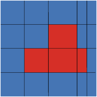
Figure 5: Partitioned block structure on regression coefficients.

Then,

$$Q(\boldsymbol{\beta})=L(\boldsymbol{\beta})+\mathcal{P}(\boldsymbol{\beta}),\qquad Q^{\mathcal{A}}(\alpha)=L^{\mathcal{A}}(\alpha)+\mathcal{P}^{\mathcal{A}}(\alpha).$$

Let $\mathcal{M}_{\mathcal{A}}$ denote the set of $\mathbb{R}^{NTP}$ coefficients that have block structure and $T:\mathcal{M}_{\mathcal{A}}\longmapsto\mathbb{R}^{LP}$ be the mapping that $T(\boldsymbol{\beta})$ is the $LP\times 1$ vector consisting of $L$ vectors with dimension $P$ and its $l$th vector is the values for the $l$th block. Let $T^{*}:\mathbb{R}^{NTP}\longmapsto\mathbb{R}^{LP}$ be the mapping that $T^{*}(\boldsymbol{\beta})=\{|\mathcal{A}_{l}|^{-1}\sum_{(i,t)\in\mathcal{A}_{l}}\beta_{it}^{\top},l=1,\cdots,L\}$. In the following, we consider the neighborhood of $\boldsymbol{\beta^{0}}$, $\Theta_{1}=\{\boldsymbol{\beta}\in\mathbb{R}^{NTP}:\sup_{it}\left\|\beta_{it}-\beta_{it}^{0}\right\|\leq\Delta_{n}\}$.

It is obvious that when $\boldsymbol{\beta}\in\mathcal{M}_{\mathcal{A}}$, $T(\boldsymbol{\beta})=T^{*}(\boldsymbol{\beta})$. By calculation, $\mathcal{P}(\boldsymbol{\beta})=\mathcal{P}^{\mathcal{A}}(T(\boldsymbol{\beta}))$ for every $\boldsymbol{\beta}\in\mathcal{M}_{\mathcal{A}}$ and $\mathcal{P}(T^{-1}(\alpha))=\mathcal{P}^{\mathcal{A}}(\alpha)$ according to split structure as shown in Figure 5. Therefore, we conclude that

$$Q(\boldsymbol{\beta})=Q^{\mathcal{A}}(T(\boldsymbol{\beta})),\qquad Q^{\mathcal{A}}(\alpha)=Q(T^{-1}(\alpha)).$$ (A.3)

We will verify the Theorem 2 by two steps.

The first step:

For any $\boldsymbol{\beta}\in\mathbb{R}^{NTP}$, Let $T^{*}(\boldsymbol{\beta})=\alpha$ and $\boldsymbol{\beta}^{*}=T^{-1}(T^{*}(\boldsymbol{\beta}))=\left(\boldsymbol{\beta}_{11}^{*\top},\cdots,\boldsymbol{\beta}_{1T}^{*\top},\cdots,\boldsymbol{\beta}_{N1}^{*\top},\cdots,\boldsymbol{\beta}_{NT}^{*\top}\right)^{*\top}$. Since

$$\left\|\alpha_{l}-\alpha_{l^{\prime}}\right\|\geq\left\|\alpha_{l}^{0}-\alpha_{l^{\prime}}^{0}\right\|-2\sup_{l}\left\|\alpha_{l}-\alpha_{l}^{0}\right\|$$

and

$$\sup_{l}\left\|\alpha_{l}-\alpha_{l}^{0}\right\|^{2} =\sup_{l}\left\|\left|\mathcal{A}_{l}\right|^{-1}\sum_{(i,t)\in\mathcal{A}_{l}}\beta_{it}-\alpha_{l}^{0}\right\|^{2}=\sup_{l}\left\|\left|\mathcal{A}_{l}\right|^{-1}\sum_{(i,t)\in\mathcal{A}_{l}}\left(\beta_{it}-\beta_{it}^{0}\right)\right\|^{2}$$

$$=\sup_{l}\left|\mathcal{A}_{l}\right|^{-2}\left\|\sum_{(i,t)\in\mathcal{A}_{l}}\left(\beta_{it}-\beta_{it}^{0}\right)\right\|^{2}\leq\sup_{l}\left|\mathcal{A}_{l}\right|^{-1}\sum_{(i,t)\in\mathcal{A}_{l}}\left\|\left(\beta_{it}-\beta_{it}^{0}\right)\right\|^{2}$$

$$\leq\sup_{(i,t)}\left\|\beta_{it}-\beta_{it}^{0}\right\|^{2}\leq\Delta_{n}^{2},$$

then, for all $l$ and $l^{\prime}$

$$\left\|\alpha_{l}-\alpha_{l^{\prime}}\right\|\geq\left\|\alpha_{l}^{0}-\alpha_{l^{\prime}}^{0}\right\|-2\sup_{l}\left\|\alpha_{l}-\alpha_{l}^{0}\right\|\geq b-2\Delta_{n}.$$

By the assumption that $b>a\lambda\gg\Delta_{n}$ and $b>a^{\prime}\gamma\gg\Delta_{n}$, we can get that $b-2\Delta_{n}>a\lambda$, $b-2\Delta_{n}>a^{\prime}\gamma$. As a result, we have $\mathcal{P}^{\mathcal{A}}(T^{*}(\boldsymbol{\beta}))=\mathcal{C}$, where $\mathcal{C}$ is a constant,under the assumption. Furthermore, $Q^{\mathcal{A}}(T^{*}(\boldsymbol{\beta}))=L^{\mathcal{A}}(T^{*}(\boldsymbol{\beta}))+\mathcal{C}$.

Because that $\widetilde{\alpha}$ is the unique global minimizer of $L^{\mathcal{A}}(\alpha)$, $L^{\mathcal{A}}(T^{*}(\boldsymbol{\beta}))>L^{\mathcal{A}}(\widetilde{\alpha})$. Furthermore, $Q^{\mathcal{A}}(T^{*}(\boldsymbol{\beta}))>Q^{\mathcal{A}}(\widetilde{\alpha})$. Implied by (A.3) that $Q^{\mathcal{A}}(\widetilde{\alpha})=Q(\widetilde{\boldsymbol{\beta}})$ and $Q^{\mathcal{A}}(T^{*}(\boldsymbol{\beta}))=Q(T^{-1}(T^{*}(\boldsymbol{\beta})))=Q(\boldsymbol{\beta}^{*})$. Finally, $Q(\boldsymbol{\beta}^{*})>Q(\widetilde{\boldsymbol{\beta}})$ for all $\boldsymbol{\beta}^{*}\neq\widetilde{\boldsymbol{\beta}}$.

The second step:

For a positive sequence $t$, let $\Theta_{2}=\{\beta_{it}:\sup_{it}\left\|\beta_{it}-\tilde{\beta}_{it}\right\|\leq t\}$. For $\boldsymbol{\beta}\in\Theta_{1}\cap\Theta_{2}$, By the Taylor expansion around $\boldsymbol{\beta}_{it}$, we can divide the difference of objective function into three parts:

$$Q(\boldsymbol{\beta})-Q(\boldsymbol{\beta}^{*})=\Gamma_{1}+\Gamma_{2}+\Gamma_{3}$$ (A.4)

where

$$\Gamma_{1}=-(\boldsymbol{Y}-\boldsymbol{X}\boldsymbol{\beta}^{m})^{\top}\boldsymbol{X}(\boldsymbol{\beta}-\boldsymbol{\beta}^{*}),$$

$$\Gamma_{2}=\sum_{t=1}^{T}\sum_{i=1}^{N}\frac{\partial\mathcal{P}(\boldsymbol{\beta}^{m})}{\partial\boldsymbol{\beta}_{it}}(\boldsymbol{\beta}_{it}-\boldsymbol{\beta}_{it}^{*}),$$

$$\Gamma_{3}=\sum_{i=1}^{N}\sum_{t=1}^{T}\frac{\partial\mathcal{P}(\boldsymbol{\beta}^{m})}{\partial\boldsymbol{\beta}_{t}}(\boldsymbol{\beta}_{it}-\boldsymbol{\beta}_{it}^{*}),$$

and $\boldsymbol{\beta}_{i}=(\beta_{i1}^{\top},\beta_{i2}^{\top},\cdots,\beta_{iT}^{\top})^{\top}$, $\boldsymbol{\beta}_{t}=(\beta_{1t}^{\top},\beta_{2t}^{\top},\cdots,\beta_{Nt}^{\top})^{\top}$, $\boldsymbol{\beta}^{m}=\theta\boldsymbol{\beta}+(1-\theta)\boldsymbol{\beta}^{*}$.

$$\Gamma_{2} = \sum_{t=1}^{T}\sum_{i<j}\mathcal{P}_{\lambda}\left(\left\|\boldsymbol{\beta}_{it}^{m}-\boldsymbol{\beta}_{jt}^{m}\right\|\right)-\sum_{t=1}^{T}\sum_{i<j}\mathcal{P}_{\lambda}\left(\left\|\boldsymbol{\beta}_{it}^{*}-\boldsymbol{\beta}_{jt}^{*}\right\|\right)$$

$$= \lambda\sum_{t=1}^{T}\sum_{i<j}\left[\rho\left(\left\|\boldsymbol{\beta}_{it}^{m}-\boldsymbol{\beta}_{jt}^{m}\right\|\right)-\rho\left(\left\|\boldsymbol{\beta}_{it}^{*}-\boldsymbol{\beta}_{jt}^{*}\right\|\right)\right]$$

$$= \lambda\sum_{t=1}^{T}\sum_{i<j}\left\{\left[\frac{\partial\rho\left(\left\|\boldsymbol{\beta}_{it}^{m}-\boldsymbol{\beta}_{jt}^{m}\right\|\right)}{\partial\boldsymbol{\beta}_{it}}\right]^{\prime}\left(\boldsymbol{\beta}_{it}-\boldsymbol{\beta}_{it}^{*}\right)+\left[\frac{\partial\rho\left(\left\|\boldsymbol{\beta}_{it}^{m}-\boldsymbol{\beta}_{jt}^{m}\right\|\right)}{\partial\boldsymbol{\beta}_{jt}}\right]^{\prime}\left(\boldsymbol{\beta}_{jt}-\boldsymbol{\beta}_{jt}^{*}\right)\right\}.$$

Since

$$\frac{\partial\rho\left(\left\|\boldsymbol{\beta}_{it}^{m}-\boldsymbol{\beta}_{jt}^{m}\right\|\right)}{\partial\boldsymbol{\beta}_{it}} = \rho^{\prime}\left(\left\|\boldsymbol{\beta}_{it}^{m}-\boldsymbol{\beta}_{jt}^{m}\right\|\right)\frac{\partial\left\|\boldsymbol{\beta}_{it}^{m}-\boldsymbol{\beta}_{jt}^{m}\right\|}{\partial\boldsymbol{\beta}_{it}}$$

$$= \rho^{\prime}\left(\left\|\boldsymbol{\beta}_{it}^{m}-\boldsymbol{\beta}_{jt}^{m}\right\|\right)\left\|\boldsymbol{\beta}_{it}^{m}-\boldsymbol{\beta}_{jt}^{m}\right\|^{-1}\frac{\partial\left[\left\|\boldsymbol{\beta}_{it}^{m}-\boldsymbol{\beta}_{jt}^{m}\right\|^{2}\right]}{\partial\boldsymbol{\beta}_{it}}$$

$$= \rho^{\prime}\left(\left\|\boldsymbol{\beta}_{it}^{m}-\boldsymbol{\beta}_{jt}^{m}\right\|\right)\left\|\boldsymbol{\beta}_{it}^{m}-\boldsymbol{\beta}_{jt}^{m}\right\|^{-1}\left(\boldsymbol{\beta}_{it}^{m}-\boldsymbol{\beta}_{jt}^{m}\right)^{\top}$$

So we have

$$\Gamma_{2}=\sum_{t=1}^{T}\sum_{i<j}\left\{\rho^{\prime}\left(\left\|\boldsymbol{\beta}_{it}^{m}-\boldsymbol{\beta}_{jt}^{m}\right\|\right)\left\|\boldsymbol{\beta}_{it}^{m}-\boldsymbol{\beta}_{jt}^{m}\right\|^{-1}\left(\boldsymbol{\beta}_{it}^{m}-\boldsymbol{\beta}_{jt}^{m}\right)^{\top}\left[\left(\boldsymbol{\beta}_{it}-\boldsymbol{\beta}_{it}^{*}\right)+\left(\boldsymbol{\beta}_{jt}-\boldsymbol{\beta}_{jt}^{*}\right)\right]\right\}$$

When $(i,t),(j,t)\in\mathcal{\mathcal{A}}_{l},\boldsymbol{\beta}_{it}^{*}=\boldsymbol{\beta}_{jt}^{*}$ and $\boldsymbol{\beta}_{it}^{m}-\boldsymbol{\beta}_{jt}^{m}=\theta\left(\boldsymbol{\beta}_{it}-\boldsymbol{\beta}_{jt}\right)$ ,

$$\Gamma_{2}= \lambda\sum_{t=1}^{T}\sum_{l=1}^{L}\sum_{\begin{subarray}{c}(i,t),(j,t)\in\mathcal{A}_{l}\\ i<j\end{subarray}}\rho^{\prime}\left(\left\|\beta_{it}^{m}-\beta_{jt}^{m}\right\|\right)\left\|\beta_{it}^{m}-\beta_{jt}^{m}\right\|^{-1}\left(\beta_{it}^{m}-\beta_{jt}^{m}\right)^{\mathrm{T}}\left(\beta_{it}-\beta_{jt}\right)$$

$$+ \lambda\sum_{t=1}^{T}\sum_{l<l^{\prime}}\sum_{\begin{subarray}{c}(i,t)\in\mathcal{A}_{l}\\ (j,t)\in\mathcal{A}_{l^{\prime}}\end{subarray}}\rho^{\prime}\left(\left\|\beta_{it}^{m}-\beta_{jt}^{m}\right\|\right)\left\|\beta_{it}^{m}-\beta_{jt}^{m}\right\|^{-1}\left(\beta_{it}^{m}-\beta_{jt}^{m}\right)^{\top}\left\{\left(\beta_{it}-\beta_{it}^{*}\right)-\left(\beta_{jt^{\prime}}-\beta_{jt}^{*}\right)\right\}.$$

Moreover,

$$\sup_{(i,t)}\left\|\beta_{it}^{*}-\beta_{it}^{0}\right\|^{2}=\sup_{l}\left\|\alpha_{l}-\alpha_{l}^{0}\right\|^{2}\leq\Delta_{n}^{2},$$

and

$$\sup_{(i,t)}\left\|\beta_{it}^{m}-\beta_{it}^{0}\right\|\leq\theta\sup_{(i,t)}\|\beta_{it}-\beta_{it}^{0}\|+(1-\theta)\sup_{(i,t)}\|\beta_{it}^{*}-\beta_{it}^{0}\|\leq\theta\Delta_{n}+(1-\theta)\Delta_{n}=\Delta_{n}.$$

Hence, for $l\neq l^{\prime},(i,t)\in\mathcal{A}_{l},(j,t)\in\mathcal{A}_{l^{\prime}}$,

$$\left\|\beta_{it}^{m}-\beta_{jt}^{m}\right\|\geq\min_{(i,t)\in\mathcal{A}_{l},(j,t)\in\mathcal{A}_{l^{\prime}}}\left\|\beta_{it}^{0}-\beta_{jt}^{0}\right\|-2\max_{(i,t)}\left\|\beta_{it}^{m}-\beta_{it}^{0}\right\|\geq b-2\Delta_{n}>a\lambda,$$

and thus $\rho^{\prime}\left(\left\|\beta_{it}^{m}-\beta_{jt}^{m}\right\|\right)=0$. Therefore,

$$\Gamma_{2}= \lambda\sum_{t=1}^{T}\sum_{l=1}^{L}\sum_{\begin{subarray}{c}(i,t),(j,t)\in\mathcal{A}_{l}\\ i<j\end{subarray}}\rho^{\prime}\left(\left\|\beta_{it}^{m}-\beta_{jt}^{m}\right\|\right)\left\|\beta_{it}^{m}-\beta_{jt}^{m}\right\|^{-1}\left(\beta_{it}^{m}-\beta_{jt}^{m}\right)^{\mathrm{T}}\left(\beta_{it}-\beta_{jt}\right)$$

$$= \lambda\sum_{t=1}^{T}\sum_{l=1}^{L}\sum_{\begin{subarray}{c}(i,t),(j,t)\in\mathcal{A}_{l}\\ i<j\end{subarray}}\rho^{\prime}\left(\left\|\beta_{it}^{m}-\beta_{jt}^{m}\right\|\right)\left\|\beta_{it}-\beta_{jt}\right\|.$$

With that $\sup_{(i,t)}\|\beta_{it}^{*}-\widetilde{\beta}_{it}\|\leq\sup_{(i,t)}\|\beta_{it}-\widetilde{\beta}_{it}\|$, we can obtain

$$\sup_{(i,t)}\left\|\beta_{it}^{m}-\beta_{jt^{\prime}}^{m}\right\| \leq 2\sup_{(i,t)}\left\|\beta_{it}^{m}-\beta_{it}^{*}\right\|\leq 2\sup_{i}\left\|\beta_{it}-\beta_{it}^{*}\right\|$$

$$\leq 2\left\{\sup_{(i,t)}\|\beta_{it}-\widetilde{\beta}_{it}\|+\sup_{(i,t)}\|\beta_{it}^{*}-\widetilde{\beta}_{it}\|\right\}\leq 4\sup_{(i,t)}\left\|\beta_{it}-\widetilde{\beta}_{it}\right\|\leq 4t.$$

Therefore, $\rho^{\prime}\left(\left\|\beta_{it}^{m}-\beta_{jt}^{m}\right\|\right)\geq\rho^{\prime}\left(4t\right)$, and by concavity of $\rho(\cdot)$,

$$\Gamma_{2}\geq\lambda\sum_{t=1}^{T}\sum_{l=1}^{L}\sum_{\begin{subarray}{c}(i,t),(j,t)\in\mathcal{A}_{l}\\ i<j\end{subarray}}\rho^{\prime}\left(4t\right)\left\|\beta_{it}-\beta_{jt}\right\|$$ (A.5)

Similarly,

$$\Gamma_{3}\geq\gamma\sum_{i=1}^{N}\sum_{l=1}^{L}\sum_{\begin{subarray}{c}(i,t),(i,t^{\prime})\in\mathcal{A}_{l}\\ t<t^{\prime}\end{subarray}}\rho^{\prime}\left(4t\right)\left\|\beta_{it}-\beta_{it}\right\|.$$ (A.6)

Let,

$$\boldsymbol{Q}=\left(\boldsymbol{Q}_{1}^{\top},\ldots,\boldsymbol{Q}_{NT}^{\top}\right)^{\top}=\left[\left(\boldsymbol{Y}-\mathbf{X}\boldsymbol{\beta}^{m}\right)^{\top}\boldsymbol{X}\right]^{\top},$$

then

$$\Gamma_{1} =-\boldsymbol{Q}^{\top}\left(\boldsymbol{\beta}-\boldsymbol{\beta}^{*}\right)=-\sum_{l=1}^{L}\sum_{\left\{(i,t),(j,t^{\prime})\in\mathcal{A}_{l}\right\}}\frac{\boldsymbol{Q}_{it}^{\top}\left(\beta_{it}-\beta_{jt^{\prime}}\right)}{\left|\mathcal{A}_{l}\right|}$$

$$=-\sum_{l=1}^{L}\sum_{\left\{(i,t),(j,t^{\prime})\in\mathcal{A}_{l}\right\}}\frac{\boldsymbol{Q}_{it}^{\top}\left(\beta_{it}-\beta_{jt^{\prime}}\right)}{2\left|\mathcal{A}_{l}\right|}-\sum_{l=1}^{L}\sum_{\left\{(i,t),(j,t^{\prime})\in\mathcal{A}_{l}\right\}}\frac{\boldsymbol{Q}_{it}^{\top}\left(\beta_{it}-\beta_{jt^{\prime}}\right)}{2\left|\mathcal{A}_{l}\right|}$$

$$=-\sum_{l=1}^{L}\sum_{\left\{(i,t),(j,t^{\prime})\in\mathcal{A}_{l}\right\}}\frac{\left(\boldsymbol{Q}_{jt^{\prime}}-\boldsymbol{Q}_{it}\right)^{\top}\left(\beta_{jt^{\prime}}-\beta_{it}\right)}{2\left|\mathcal{A}_{l}\right|}$$

$$=-\sum_{l=1}^{L}\sum_{\begin{subarray}{c}(i,t),(j,t^{\prime})\in\mathcal{A}_{l}\\ i<j,t<t^{\prime}\end{subarray}}\frac{\left(\mathbf{Q}_{jt^{\prime}}-\boldsymbol{Q}_{it}\right)^{\top}\left(\beta_{jt^{\prime}}-\beta_{it}\right)}{\left|\mathcal{A}_{l}\right|}.$$

Moreover,

$$\boldsymbol{Q}_{it}=\left(y_{it}-x_{it}^{\top}\beta_{it}^{m}\right)x_{it}=\left(\epsilon_{it}+x_{it}^{\top}\left(\beta_{it}^{0}-\beta_{it}^{m}\right)\right)x_{it}$$

and

$$\sup_{(i,t)}\left\|\boldsymbol{Q}_{it}\right\|\leq\sup_{(i,t)}\left\{\left\|x_{it}\right\|\left(\|\epsilon\|_{\infty}+\left\|x_{it}\right\|\left\|\beta_{it}^{0}-\beta_{it}^{m}\right\|\right)\right\},$$

then

$$\sup_{(i,t)}\left\|\boldsymbol{Q}_{it}\right\|\leq c_{4}\sqrt{P}\left(\|\epsilon\|_{\infty}+c_{4}\sqrt{P}\Delta_{n}\right).$$

By condition (C2),

$$P\left(\|\epsilon\|_{\infty}>\sqrt{2c_{1}^{-1}}\sqrt{\log(NT)}\right)\leq\sum_{i=1}^{N}\sum_{t=1}^{T}P\left(\left|\epsilon_{it}\right|>\sqrt{2c_{1}^{-1}}\sqrt{\log(NT)}\right)\leq 2(NT)^{-1}.$$

Then

$$\sup_{(i,t)}\left\|\boldsymbol{Q}_{it}\right\|\leq c_{4}\sqrt{P}\left(\sqrt{2c_{1}^{-1}}\sqrt{\log(NT)}+c_{4}\sqrt{P}\Delta_{n}\right)$$

and

$$\frac{\left(\mathbf{Q}_{jt^{\prime}}-\boldsymbol{Q}_{it}\right)^{\top}\left(\boldsymbol{\beta}_{jt^{\prime}}-\boldsymbol{\beta}_{it}\right)}{\left|\mathcal{A}_{l}\right|}$$

$$\leq\left|\mathcal{A}_{\min}\right|^{-1}\left\|\boldsymbol{Q}_{jt^{\prime}}-\boldsymbol{Q}_{it}\right\|\left\|\beta_{it}-\beta_{jt^{\prime}}\right\|\leq\left|\mathcal{A}_{\min}\right|^{-1}2\sup_{it}\left\|\boldsymbol{Q}_{it}\right\|\left\|\beta_{it}-\beta_{jt^{\prime}}\right\|$$

$$\leq 2\left|\mathcal{A}_{\min}\right|^{-1}c_{4}\sqrt{P}\left(\sqrt{2c_{1}^{-1}}\sqrt{\log(NT)}+c_{4}\sqrt{P}\Delta_{n}\right)\left\|\beta_{it}-\beta_{jt^{\prime}}\right\|.$$ (A.7)

At last, we have

$$\boldsymbol{Q}(\boldsymbol{\beta})-\boldsymbol{Q}(\boldsymbol{\beta}^{*}) \geq \sum_{l=1}^{L}\left[\sum_{t=1}^{T}\sum_{\begin{subarray}{c}(i,t),(j,t)\in\mathcal{A}_{l}\\ i<j\end{subarray}}\lambda\rho^{\prime}(4t)\left\|\beta_{it}-\beta_{jt^{\prime}}\right\|+\sum_{i=1}^{N}\sum_{\begin{subarray}{c}(i,t),(i,t^{\prime})\in\mathcal{A}_{l}\\ t<t^{\prime}\end{subarray}}\gamma\rho^{\prime}(4t)\right]\left\|\beta_{it}-\beta_{jt^{\prime}}\right\|-$$

$$\sum_{l=1}^{L}\sum_{\begin{subarray}{c}(i,t),(j,t^{\prime})\in\mathcal{A}_{l}\\ i<j,t<t^{\prime}\end{subarray}}2\left|\mathcal{A}_{\min}\right|^{-1}c_{4}\sqrt{P}\left(\sqrt{2c_{1}^{-1}}\sqrt{\log(NT)}+c_{4}\sqrt{P}\Delta_{n}\right)\left\|\beta_{it}-\beta_{jt^{\prime}}\right\|$$

$$\geq \sum_{l=1}^{L}\sum_{\begin{subarray}{c}(i,t),(j,t^{\prime})\in\mathcal{A}_{l}\\ i<j,t<t^{\prime}\end{subarray}}min(\lambda,\gamma)\rho^{\prime}(4t)\left\|\beta_{it}-\beta_{jt^{\prime}}\right\|-$$

$$\sum_{l=1}^{L}\sum_{\begin{subarray}{c}(i,t),(j,t^{\prime})\in\mathcal{A}_{l}\\ i<j,t<t^{\prime}\end{subarray}}2\left|\mathcal{A}_{\min}\right|^{-1}c_{4}\sqrt{P}\left(\sqrt{2c_{1}^{-1}}\sqrt{\log(NT)}+c_{4}\sqrt{P}\Delta_{n}\right)\left\|\beta_{it}-\beta_{jt^{\prime}}\right\|.$$

If $t=o(1)$, then $\rho^{\prime}(4t)\rightarrow 1$. Since $\lambda\gg\Delta_{n}$, $\gamma\gg\Delta_{n}$, $P=o(NT)$, and $|\mathcal{A}_{min}|^{-1}P=o(1)$, then $min(\lambda,\gamma)\gg\left|\mathcal{A}_{\min}\right|^{-1}\sqrt{P\log(NT)}$ and $min(\lambda,\gamma)\gg\left|\mathcal{A}_{\min}\right|^{-1}P\Delta_{n}$. Therefore, $\boldsymbol{Q}(\boldsymbol{\beta})-\boldsymbol{Q}(\boldsymbol{\beta}^{*})\geq 0$, if $N$ or $T$ tend towards infinity.

Proof of COROLLARY 1

According to asymptotic equivalence, we can conclude COROLLARY 1 based on Theorem 1 and Theorem 2. Besides, we can also get $\hat{L}\overset{p}{\rightarrow}L^{0}$.

According to assumption (C2) (iv) $\left|\mathcal{A}_{\min}\right|\gg(LP)^{1/2}(NT)^{3/4}$, we can get $L^{0}P=o_{p}\left(\frac{1}{(NT)^{1/6}}\right)$. Thus,

$${\displaystyle\lim_{(N,T)\to\infty}\hat{\sigma}^{2}={\displaystyle\lim_{(N,T)\to\infty}\frac{\boldsymbol{\epsilon}^{\top}\boldsymbol{\epsilon}}{NT}-{\displaystyle\lim_{(N,T)\to\infty}\frac{\boldsymbol{\epsilon}^{\top}\boldsymbol{X}}{NT}\left(\frac{\boldsymbol{X}^{\top}\boldsymbol{X}}{NT}\right)^{-1}\frac{\boldsymbol{X}^{\top}\boldsymbol{\epsilon}}{NT}}}}.$$

According to assumption (C1) and assumption (C2) that $\frac{\boldsymbol{X}^{\top}\boldsymbol{\epsilon}}{NT}\overset{p}{\rightarrow}0$ and $\frac{\boldsymbol{X}^{\top}\boldsymbol{X}}{NT}=O_{p}(1)$, as $(N,T)\to\infty$ , $\hat{\sigma}^{2}\overset{p}{\rightarrow}\sigma^{2}$ is obtained.

References

• (1)
• Bai (2010) Bai, Jushan. 2010. “Common breaks in means and variances for panel data.” Journal of Econometrics 157 (1): 78–92.
• Baltagi et al. (2016) Baltagi, Badi H., Qu Feng, and Chihwa Kao. 2016. “Estimation of heterogeneous panels with structural breaks.” Journal of Econometrics 191 (1): 176–195.
• Belzil and Hansen (2002) Belzil, Christian, and Jörgen Hansen. 2002. “Unobserved ability and the return to schooling.” Econometrica 70 (5): 2075–2091.
• Bester and Hansen (2016) Bester, C. Alan, and Christian B. Hansen. 2016. “Grouped effects estimators in fixed effects models.” Journal of Econometrics 190 (1): 197–208.
• Boneva et al. (2015) Boneva, Lena, Oliver Linton, and Michael Vogt. 2015. “A semiparametric model for heterogeneous panel data with fixed effects.” Journal of Econometrics 188 (2): 327–345.
• Bonhomme and Manresa (2015) Bonhomme, Stéphane, and Elena Manresa. 2015. “Grouped Patterns of Heterogeneity in Panel Data.” Econometrica 83 (3): 1147–1184.
• Browning and Carro (2010) Browning, Martin, and Jesus M Carro. 2010. “Heterogeneity in dynamic discrete choice models.” The Econometrics Journal 13 (1): 1–39.
• Chernozhukov et al. (2018) Chernozhukov, Victor, Christian Hansen, Yuan Liao, and Yinchu Zhu. 2018. “Inference for Heterogeneous Effects using Low-Rank Estimation of Factor Slopes.” arXiv preprint arXiv:1812.08089.
• Chudik et al. (2011) Chudik, Alexander, M. Hashem Pesaran, and Elisa Tosetti. 2011. “Weak and strong cross-section dependence and estimation of large panels.” The Econometrics Journal 14 (1): C45–C90.
• Cornett et al. (2011) Cornett, Marcia Millon, Jamie John McNutt, Philip E Strahan, and Hassan Tehranian. 2011. “Liquidity risk management and credit supply in the financial crisis.” Journal of Financial Economics 101 (2): 297–312.
• Fan and Li (2001) Fan, Jianqing, and Runze Li. 2001. “Variable Selection via Nonconcave Penalized Likelihood and its Oracle Properties.” Journal of the American Statistical Association 96 (456): 1348–1360.
• Feng et al. (2017) Feng, Guohua, Jiti Gao, Bin Peng, and Xiaohui Zhang. 2017. “A varying-coefficient panel data model with fixed effects: Theory and an application to US commercial banks.” Journal of Econometrics 196 (1): 68–82.
• Huang et al. (2018) Huang, Wenxin, Peter C. B. Phillips, and Liangjun Su. 2018. “Nonstationary Panel Model with Latent Group Structures and Cross-sectional Dependence.” Working Paper.
• Karabiyik et al. (2017) Karabiyik, Hande, Jean-Pierre Urbain, and Joakim Westerlund. 2017. “CCE estimation of factor-augmented regression models with more factors than observables.” Journal of Applied Econometrics 0 (0): .
• Kasahara and Shimotsu (2009) Kasahara, Hiroyuki, and Katsumi Shimotsu. 2009. “Nonparametric identification of finite mixture models of dynamic discrete choices.” Econometrica 77 (1): 135–175.
• Kim (2011) Kim, Dukpa. 2011. “Estimating a common deterministic time trend break in large panels with cross sectional dependence.” Journal of Econometrics 164 (2): 310–330.
• Li et al. (2011) Li, Degui, Jia Chen, and Jiti Gao. 2011. “Non-parametric time-varying coefficient panel data models with fixed effects.” The Econometrics Journal 14 (3): 387–408.
• Li et al. (2017) Li, Degui, Junhui Qian, and Liangjun Su. 2017. “Panel Data Models With Interactive Fixed Effects and Multiple Structural Breaks.” Journal of the American Statistical Association 111 (516): 1804–1819.
• Lu and Su (2019) Lu, Xun, and Liangjun Su. 2019. “Uniform Inference in Linear Panel Data Models with Two-Dimensional Heterogeneity.” Working Paper.
• Lumsdaine et al. (2020) Lumsdaine, Robin L, Ryo Okui, and Wendun Wang. 2020. “Estimation of Panel Group Structure Models with Structural Breaks in Group Memberships and Coefficients.” Available at SSRN 3617416.
• Ma and Huang (2016) Ma, Shujie, and Jian Huang. 2016. “Estimating subgroup-specific treatment effects via concave fusion.” arXiv preprint arXiv:1607.03717.
• Ma and Huang (2017) Ma, Shujie, and Jian Huang. 2017. “A Concave Pairwise Fusion Approach to Subgroup Analysis.” Journal of the American Statistical Association 112 (517): 410–423.
• Murtazashvili and Wooldridge (2008) Murtazashvili, Irina, and Jeffrey M Wooldridge. 2008. “Fixed effects instrumental variables estimation in correlated random coefficient panel data models.” Journal of Econometrics 142 (1): 539–552.
• Neal (2018) Neal, Timothy. 2018. “Multidimensional Slope Heterogeneity in Panel Data Models.” UNSW Business School Research Paper (2016-15A): .
• Okui and Wang (2020) Okui, Ryo, and Wendun Wang. 2020. “Heterogeneous structural breaks in panel data models.” Journal of Econometrics.
• Pei et al. (2018) Pei, Youquan, Tao Huang, and Jinhong You. 2018. “Nonparametric fixed effects model for panel data with locally stationary regressors.” Journal of Econometrics 202 (2): 286–305.
• Pesaran (2006) Pesaran, M. Hashem. 2006. “Estimation and Inference in Large Heterogeneous Panels with a Multifactor Error Structure.” Econometrica 74 (4): 967–1012.
• Qian and Su (2016) Qian, Junhui, and Liangjun Su. 2016. “Shrinkage estimation of common breaks in panel data models via adaptive group fused Lasso.” Journal of Econometrics 191 (1): 86–109.
• Smith (2018) Smith, Simon. 2018. “Forecasting Panel Data with Structural Breaks and Regime-Specific Grouped Heterogeneity.” USC-INET Research Paper (18-20): .
• Su and Ju (2018) Su, Liangjun, and Gaosheng Ju. 2018. “Identifying latent grouped patterns in panel data models with interactive fixed effects.” Journal of Econometrics 206 (2): 554–573.
• Su et al. (2016) Su, Liangjun, Zhentao Shi, and Peter C. B. Phillips. 2016. “Identifying Latent Structures in Panel Data.” Econometrica 84 (6): 2215–2264.
• Su et al. (2019) Su, Liangjun, Xia Wang, and Sainan Jin. 2019. “Sieve estimation of time-varying panel data models with latent structures.” Journal of Business & Economic Statistics 37 (2): 334–349.
• Tibshirani et al. (2005) Tibshirani, Robert, Michael Saunders, Saharon Rosset, Ji Zhu, and Keith Knight. 2005. “Sparsity and smoothness via the fused lasso.” Journal of the Royal Statistical Society: Series B (Statistical Methodology) 67 (1): 91–108.
• Vogt and Linton (2017) Vogt, Michael, and Oliver Linton. 2017. “Classification of non-parametric regression functions in longitudinal data models.” Journal of the Royal Statistical Society: Series B (Statistical Methodology) 79 (1): 5–27.
• Wang et al. (2009) Wang, Hansheng, Bo Li, and Chenlei Leng. 2009. “Shrinkage tuning parameter selection with a diverging number of parameters.” Journal of the Royal Statistical Society: Series B (Statistical Methodology) 71 (3): 671–683.
• Wang et al. (2018) Wang, Wuyi, Peter C. B. Phillips, and Liangjun Su. 2018. “Homogeneity pursuit in panel data models: Theory and application.” Journal of Applied Econometrics 33 (6): 797–815.
• Wooldridge (2005) Wooldridge, Jeffrey M. 2005. “Fixed-effects and related estimators for correlated random-coefficient and treatment-effect panel data models.” Review of Economics and Statistics 87 (2): 385–390.
• Zhang (2010) Zhang, Cun-Hui. 2010. “NEARLY UNBIASED VARIABLE SELECTION UNDER MINIMAX CONCAVE PENALTY.” The Annals of Statistics 38 (2): 894–942.