Spin-orbit interactions may relax the rigid conditions leading to flat bands

Abstract

Flat bands are of extreme interest in a broad spectrum of fields since given by their high degeneracy, a small perturbation introduced in the system is able to push the ground state in the direction of an ordered phase of interest. Hence the flat band engineering in real materials attracts huge attention. However, manufacturing a flat band represents a difficult task because its appearance in a real system is connected to rigid mathematical conditions relating a part of Hamiltonian parameters. Consequently, whenever a flat band is desired to be manufactured, these Hamiltonian parameters must be tuned exactly to the values fixed by these rigid mathematical conditions. Here we demonstrate that taking the many-body spin-orbit interaction (SOI) into account– which can be continuously tuned e.g. by external electric fields –, these rigid mathematical conditions can be substantially relaxed. On this line we show that a $\sim 20-30\%$ variation in the Hamiltonian parameters rigidly fixed by the flat band conditions can also lead to flat bands in the same or in a bit displaced position on the energy axis. This percentage can even increase to $\sim 80\%$ in the presence of an external magnetic field. The study is made in the case of conducting polymers. These systems are relevant not only because they have broad application possibilities, but also because they can be used to present the mathematical background of the flat band conditions in full generality, in a concise, clear and understandable manner applicable everywhere in itinerant systems.

I Introduction

Flat bands are attracting great interest today given by the broad application possibilities of the huge degeneracy they provide. Indeed, flat bands appear in several circumstances as: chiral edge mods broadband topological slow light E1 , diffraction-free photonics via collective excited states of atoms in Creutz super-radiance lattices E2 , interaction-enhanced group velocity in optical Kagome lattices E3 , production of topological states in 1D optical lattices E4 , generation of flat bands in non-Hermitian optical lattices E5 , realization of tilted Dirac cones from flat-bands which lead to intricate transport phenomena E6 , engineering flat band PT symmetric meta-materials E7 , use of singularities emerging on flat bands E8 , artificial flat band systems E9 , SQUID meta-materials on Lieb lattices E10 , or are of interest because of the emergence of different ordered phases in flat band systems as superconductivity E11 , ferromagnetism E12 , semimetal magnetic ordering E13 , excitonic insulator E14 , etc. Flat bands also produce interesting effects as quantized circular photo-galvanic effect E15 , ordered quantum dot arrays formed by moire excitons E16 , emergence of non-contractible-loop-states E17 , etc.

Flat bands occur in several type of materials from which conducting polymers E13 ; E18 ; E19 ; E20 ; E21 ; E22 have broad application possibilities covering thermal conductivity enhancement E23 , carrier charge transport E24 , heat exchangers and energy storage E25 , soft high performance capacitors E26 , switchers and commutators E27 , sensors E28 , high performance batteries E29 , biodegradable plastics E30 , light-emitting diodes E31 , organic transistors E32 , and even life sciences and medicine E33 ; E34 ; E35 . This is the reason why in the study of flat band characteristics, we exemplify the observed properties in the case of conducting polymers.

Flat bands can be effective E20 ; E36 ; E37 , or bare (i.e. provided exclusively by $\hat{H}_{kin}$, kinetic energy part of the Hamiltonian). Their main source of difficulties is that they are determined by rigid mathematical conditions connected to the parameters (e.g. hopping matrix elements, coupling constants) of the Hamiltonian ($\hat{H}$). Indeed, deducing the band structure in a lattice, in principle we obtain from the one particle part of the Hamiltonian a secular equation of the form

$$Q(\epsilon,\{p_{i}\},\{\text{trig}_{j}({\bf k}{\bf x}_{\alpha})\})=0$$ (1)

where $\epsilon=E_{n}({\bf k})$ provides the energy spectrum, $\{p_{i}\}$ represents the set of the parameters of the Hamiltonian ($i=1,2,...m_{max}$), ${\bf x}_{\alpha}$ are the Bravais vectors of the lattice, $\text{trig}_{j}(z)$ represent trigonometric functions of $\sin(nz)$, $\cos(nz)$ type (where $n$ is an integer) holding in their argument the ${\bf k}$ momentum dependence. The notation $\{\text{trig}_{j}({\bf k}{\bf x}_{\alpha})\}$ represents the set of all trigonometric functions emerging in the secular equation Eq.(1). In Eq.(1) all trigonometric contributions $\text{trig}_{j}$ emerge in Q additively, with multiplicative coefficients $T_{j}(\{p_{i}\})$ [i.e. as $V_{j}=T_{j}(\{p_{i}\})\text{trig}_{j}({\bf k}{\bf x}_{\alpha})$] which depend on the Hamiltonian parameters $\{p_{i}\}$. Eliminating these coefficients

$$T_{j}(\{p_{i}\})=0,\quad j=1,2,3,...,m$$ (2)

the ${\bf k}$ dependence disappears from the secular equation Eq.(1), hence from $Q=0$ we find ${\bf k}$ independent $\epsilon$ values, i.e. flat bands [see for exemplification Eq.(13-15)]. As seen from Eq.(2), when flat bands emerge, interdependences between Hamiltonian parameters must be present. If in Eq.(2) one has $j=1,2,...m<m_{max}$, these interdependencies rigidly fix the value of $m$ Hamiltonian parameters. Hence, when a flat band appears, only $(m_{max}-m)$ Hamiltonian parameters can be arbitrarily chosen, and $m$ Hamiltonian parameters remain rigidly fixed (given and determined by the arbitrarily taken $(m_{max}-m)$ $\hat{H}$ independent parameters). One mentions that Q in Eq.(1) contains additively also a $V_{0}=T_{j=0}$ term which does not contain ${\bf k}$, and explicitly one has $Q=\sum_{j=0}^{m}V_{j}$, [see also Eq. (25)].

Furthermore if the $T_{j}$ coefficients in Q also contain the parameter $\epsilon$, we can fix the origin of the energy axis to the position of the flat band (i.e. $\epsilon=0$), and the deduction of the flat band conditions can be similarly treated, as presented above in Eqs.(1,2).

Usually, the flat band conditions Eq.(2) are deduced from a given $\hat{H}$ describing itinerant systems with independent orbital and spin degrees of freedom. This state of facts is motivated by the observation that the many-body spin-orbit interaction $\hat{H}_{SO}=\lambda{\bf\sigma}\cdot(\nabla V\times{\bf k})$ is usually small. Here ${\bf\sigma}$ represents the spin of carriers, ${\bf k}$ is their momentum, $\nabla V$ the potential gradient, while $\lambda<<1$ is the strength of the spin-orbit interaction. When the system is interacting, (e.g. the leading term of the Coulomb interaction in a many-body system, the on-site Coulomb repulsion $U>0$ is present), the use of $H_{SO}$ introduces supplementary complications since because $\lambda<<U$ even the perturbative treatment is questionable, hence enforcing special treatment for obtaining exact results E38 ; E39 ; E40 .

Even if the spin-orbit interaction (SOI) is small, its effect is major since it breaks the spin-projection double degeneracy of each band E41 , and leads to several interesting effects as: stable soliton complexes E42 , enhances transport properties E43 , influences graphene properties E44 , coupling of Hofstadter butterfly pairs E45 , topological excitations E46 , provides stripe and plane-wave phases E47 , is able to produce spin-memory loss E48 , influences proximity effects at interfaces E49 , leads to anomalous Josephson effect E50 and condensed phases E38 . Furthermore, in several circumstances $\lambda$ is strongly tunable E51 , can be enhanced by Coulomb correlations E52 , can be increased by doping E53 , structural conformation (e.g. altering torsion in conjugated polymers) E54a , twist of the aromatic rings along the conjugation path E54b , and can be even tuned by external electric field E54 .

In this paper we show that taking into account $\hat{H}_{SO}$ in the system Hamiltonian $\hat{H}$, the rigid flat band conditions in Eq.(2) can be substantially relaxed. This procedure is tempting because the strength of SOI can be continuously tuned by an applied external electric field. Consequently, engineering a flat band in a real system is in fact more easily achievable compared to how it was considered before. As we mentioned previously, we exemplify our results on conducting polymers. Two spin-orbit couplings are considered, one (denoted by $\lambda$) as in base, and another one (denoted by $\lambda_{c}$) as inter-base contribution. In order to obtain more information, also external magnetic field is considered acting via Peierls phase factors. For the conducting polymer a pentagon chain is considered (e.g. polyaminotriazole type of chain) since this was one of the first produced conducting polymer.

The remaining part of the paper is constructed as follows: Sect. II. presents the studied system, Sect. III. deduces the band structure, and determines the flat bands, Sect. IV. (Sect. V.) describes how the mathematically rigid flat band conditions can be relaxed by spin orbit interactions maintaining (not maintaining) the position of the flat band, Sect. VI. summarizes the paper, and finally, Appendices A,B,C,D,E, containing mathematical details, close the presentation.

II The system studied

A schematic plot of the unit cell of the system containing 6 sites is presented in Fig.1. The upper antenna in the pentagon chain (as e.g. in polyaminotriazole, see Fig.2) is considered simply as the bonds (5,6) on Fig.1, since this structure is able to describe qualitatively correct its effect in the band structure. The external magnetic field is perpendicular to the plane of the cell. At the level of the Hamiltonian the system is described by

$$\hat{H}=\hat{H}_{kin}+\hat{H}_{SO}$$ (3)

where, denoting by $n=1,2,...,6$ the in-cell position of atoms, $\hat{H}_{kin}$ is given by

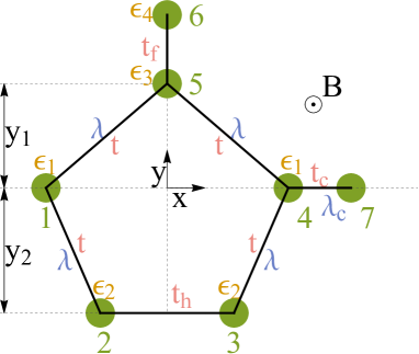
Figure 1: The pentagonal unit cell, with the nearest neighbour hopping matrix elements ($t,t_{h},t_{c},t_{f}$), the Rashba couplings ($\lambda,\lambda_{c}$), the on-site one-particle potentials ($\epsilon_{1},\epsilon_{2},\epsilon_{3},\epsilon_{4}$) and the external magnetic field ($B$).

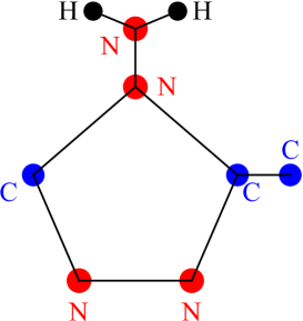
Figure 2: Schematic plot of the polyaminotriazole cell

$$\hat{H}_{kin} = \sum_{i,\sigma}[(te^{i\phi_{1,5}}\hat{c}^{\dagger}_{i,1,\sigma}\hat{c}_{i,5,\sigma^{\prime}}+te^{i\phi_{2,1}}\hat{c}^{\dagger}_{i,2,\sigma}\hat{c}_{i,1,\sigma^{\prime}}+te^{i\phi_{4,3}}\hat{c}^{\dagger}_{i,4,\sigma}\hat{c}_{i,3,\sigma^{\prime}}+te^{i\phi_{5,4}}\hat{c}^{\dagger}_{i,5,\sigma}\hat{c}_{i,4,\sigma^{\prime}}$$ (4)

$$+ t_{c}e^{i\phi_{7,4}}\hat{c}^{\dagger}_{i+a,7,\sigma}\hat{c}_{i,4,\sigma^{\prime}}+t_{h}e^{i\phi_{3,2}}\hat{c}^{\dagger}_{i,3,\sigma}\hat{c}_{i,2,\sigma}+t_{f}e^{i\phi_{6,5}}\hat{c}^{\dagger}_{i,6,\sigma}\hat{c}_{i,5,\sigma}+H.c.)$$

$$+ \sum_{n=1}^{6}\epsilon_{n}\hat{c}^{\dagger}_{i,n,\sigma}\hat{c}_{i,n,\sigma}].$$

Here $c^{\dagger}_{i,n,\sigma}$ creates an electron with $\sigma$ spin projection in the $n$ position of the cell placed at the site $i$; the $t,t_{h},t_{c},t_{f}$ are nearest neighbour hopping matrix elements; while $\epsilon_{n}$ are the on-site one-particle potentials at the in-cell positions $n$. Based on the symmetry of the unit cell, one uses the notations $\epsilon_{1}=\epsilon_{n=1}=\epsilon_{n=4},\epsilon_{2}=\epsilon_{n=2}=\epsilon_{n=3},\epsilon_{3}=\epsilon_{n=5},\epsilon_{4}=\epsilon_{n=6}$. The Peierls phase factors $\phi_{n,n^{\prime}}$ (describing the effect of the external magnetic field on the orbital motion of the carriers) are deduced in the Appendix A. Based on the obtained results, one uses the following notations $\phi_{3,2}=\phi_{1},\phi_{4,3}=\phi_{2,1}=\phi_{2},\phi_{5,4}=\phi_{1,5}=\phi_{3},\phi_{5,6}=\phi_{7,4}=0$.

Concerning $H_{SO}=\lambda{\bf\sigma}\cdot(\nabla V\times{\bf k})$, it introduces spin-flip type hoppings along the bonds of the system E38 . Since spin-orbit coupling for carbon influences considerably the physical processes in carbon made materials E55 ; E56 , we take into consideration $H_{SO}$ on bonds containing carbon atoms. This choice is supported also by the fact that these bonds provide the conjugated (i.e. conducting) nature of the polymer. From these bonds two manifolds can be constructed: in-cell bonds [(1,5);(2,1);(4,3);(5,4); see Fig.1], and inter-cell bonds [(7,4) in Fig.1]. Since the strength of the spin-orbit coupling on inter-cell bonds can be increased by atom intercalation E57 and the ending atoms on these bonds are different from the ending atoms on in-cell bonds, the SOI coupling on these bonds will be denoted by $\lambda_{c}$, while the in-cell SOI coupling by $\lambda$. In these conditions, taking into account Rashba interaction in polymers E54 , $H_{SO}$ becomes

$$\hat{H}_{SO} = \sum_{i,\sigma}(t^{\sigma,-\sigma}_{1,5}\hat{c}^{\dagger}_{i,1,\sigma}\hat{c}_{i,5,-\sigma}+t^{\sigma,-\sigma}_{2,1}\hat{c}^{\dagger}_{i,2,\sigma}\hat{c}_{i,1,-\sigma}+t^{\sigma,-\sigma}_{4,3}\hat{c}^{\dagger}_{i,4,\sigma}\hat{c}_{i,3,-\sigma}+t^{\sigma,-\sigma}_{5,4}\hat{c}^{\dagger}_{i,5,\sigma}\hat{c}_{i,4,-\sigma}$$ (5)

$$+ t_{c}^{\sigma,-\sigma}\hat{c}^{\dagger}_{i+a,7,\sigma}\hat{c}_{i,4,-\sigma}+H.c.),$$

where $\lambda=t_{5,1}^{\uparrow,\downarrow}=t_{1,5}^{\downarrow,\uparrow}=t_{1,2}^{\downarrow,\uparrow}=t_{2,1}^{\uparrow,\downarrow}=t_{3,4}^{\downarrow,\uparrow}=t_{4,3}^{\uparrow,\downarrow}=t_{4,5}^{\uparrow,\downarrow}=t_{5,4}^{\downarrow,\uparrow}$, and $\lambda_{c}=t_{c}^{\uparrow,\downarrow}=t_{7,4}^{\uparrow,\downarrow}$, furthermore $t_{i,j}^{\uparrow,\downarrow}=-t_{j,i}^{\uparrow,\downarrow}$ holds.

As mentioned previously the strength of $H_{SO}$ can be continuously tuned by an applied external electric field E58 ; E59 . One applies the external ${\bf E}=E{\vec{k}}$ field in the $z$ direction (perpendicular to the plane of the chain, ${\vec{k}}$ being the unit vector in $z$ direction). Since the carriers move in the $x$ direction (see Fig.3), the first quantized Rashba Hamiltonian becomes $\hat{H}_{R}=-i\eta\sigma_{y}k_{x}$ E60 ; E54 , (here $k_{x}$ is the momentum along the $x$ axis, i.e. along the polymer chain), hence the spin is oriented along the $y$ axis. After this step if one couples the external magnetic field ${\bf B}$ along the $z$ axis, since the magnetic induction and the spin vector are perpendicular, the Zeeman term provides zero contribution, and the external magnetic field acts only via the Peierls phase factor. If the source of SOI is exclusively the external electric field, $\lambda=\lambda_{c}$, and the connection of $\lambda$ to $E$ is given by E61

$$\lambda=\bar{K}E,\quad\bar{K}=\frac{|q|\hbar^{2}}{4m^{2}c^{2}}\frac{2\pi}{\lambda_{D}},$$ (6)

where in the expression of the coefficient $\bar{K}$, $q$ and $m$ are the charge and (rest) mass of the carriers, $\lambda_{D}$ is their de Broglie wavelength, and $c$ is the speed of light.

III The band structure

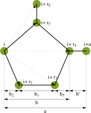
Figure 3: Notations used for the pentagonal unit cell

First we transform the $\hat{H}$ Hamiltonian from Eq.(3) to $k$-space. The fermionic operators are Fourier transformed via $\hat{c}_{i,r_{n},\sigma}=\frac{1}{\sqrt{N_{c}}}\sum_{k}e^{-ik(i+r_{n})}\hat{c}_{n,k,\sigma}$, where $N_{c}$ represents the number of unit cells and $k$ is directed along the $x$ axis (see Fig.3). One obtains [see also Eq.(A4)]

$$\hat{H}=\sum_{k}\sum_{\sigma,\sigma^{\prime}}[t^{\sigma,\sigma^{\prime}}_{1,5}\hat{c}^{\dagger}_{\bf{k},1,\sigma}\hat{c}_{\bf{k},5,\sigma^{\prime}}e^{i{\bf{k(r_{1}-r_{5}}})}+t^{\sigma,\sigma^{\prime}}_{2,1}\hat{c}^{\dagger}_{\bf{k},2,\sigma}\hat{c}_{i,1,\sigma^{\prime}}e^{i{\bf{k(r_{2}-r_{1}}})}+t^{\sigma,\sigma^{\prime}}_{4,3}\hat{c}^{\dagger}_{\bf{k},4,\sigma}\hat{c}_{\bf{k},3,\sigma^{\prime}}e^{i{\bf{k(r_{4}-r_{3}}})}$$

$$+t^{\sigma,\sigma^{\prime}}_{5,4}\hat{c}^{\dagger}_{\bf{k},5,\sigma}\hat{c}_{\bf{k},4,\sigma^{\prime}}e^{i{\bf{k(r_{5}-r_{4}}})}+t_{c}^{\sigma,\sigma^{\prime}}\hat{c}^{\dagger}_{\bf{k},1,\sigma}\hat{c}_{\bf{k},4,\sigma^{\prime}}e^{i{\bf{k(a-r_{4}}})}+t_{h}\hat{c}^{\dagger}_{\bf{k},3,\sigma}\hat{c}_{\bf{k},2,\sigma}e^{i{\bf{k(r_{3}-r_{2}}})}$$

$$+t_{f}\hat{c}^{\dagger}_{\bf{k},6,\sigma}\hat{c}_{\bf{k},5,\sigma}e^{i{\bf{k(r_{6}-r_{5}}})}+h.c.]+\sum_{n}\epsilon_{n}\hat{c}^{\dagger}_{\bf{k},n}\hat{c}_{\bf{k},n}.$$ (7)

Here $r_{n}$ represents the in-cell position of the $n$-th atoms in the cell, and $r_{1}=0$ is considered. The terms in the exponents are obtained via (see Fig.3):

$${\bf{k(r_{4}-r_{3}}})={\bf{k(r_{2}-r_{1}}})=kb_{2},\quad{\bf{k(r_{6}-r_{5}}})=0,\quad{\bf{k(a-r_{4}}})=kb^{\prime},$$

$${\bf{k(r_{3}-r_{2}}})=kb_{1},\quad{\bf{k(r_{5}-r_{4}}})={\bf{k(r_{1}-r_{5}}})=\frac{kb}{2}.$$ (8)

Using Eq.(8) in Eq.(7) one finds

$$\hat{H}=\sum_{k}\sum_{\sigma,\sigma^{\prime}}[t^{\sigma,\sigma^{\prime}}_{1,5}\hat{c}^{\dagger}_{\bf{k},1,\sigma}\hat{c}_{\bf{k},5,\sigma^{\prime}}e^{i\frac{kb}{2}}+t^{\sigma,\sigma^{\prime}}_{2,1}\hat{c}^{\dagger}_{\bf{k},2,\sigma}\hat{c}_{i,1,\sigma^{\prime}}e^{ikb_{2}}+t^{\sigma,\sigma^{\prime}}_{4,3}\hat{c}^{\dagger}_{\bf{k},4,\sigma}\hat{c}_{\bf{k},3,\sigma^{\prime}}e^{ikb_{2}}$$

$$+t^{\sigma,\sigma^{\prime}}_{5,4}\hat{c}^{\dagger}_{\bf{k},5,\sigma}\hat{c}_{\bf{k},4,\sigma^{\prime}}e^{i\frac{kb}{2}}+t_{h}\hat{c}^{\dagger}_{\bf{k},3,\sigma}\hat{c}_{\bf{k},2,\sigma}e^{ikb_{1}}+t_{f}\hat{c}^{\dagger}_{\bf{k},6,\sigma}\hat{c}_{\bf{k},5,\sigma}$$

$$+t_{c}^{\sigma,\sigma^{\prime}}\hat{c}^{\dagger}_{\bf{k},1,\sigma}\hat{c}_{\bf{k},4,\sigma^{\prime}}e^{ikb^{\prime}}+h.c.]+\sum_{n}\epsilon_{n}\hat{c}^{\dagger}_{\bf{k},n}\hat{c}_{\bf{k},n}.$$ (9)

One observes that $\hat{H}$ in Eq.(9) can be written as

$$\hat{H}=\sum_{k}[(\hat{c}^{\dagger}_{k,1,\uparrow},\ldots,\hat{c}^{\dagger}_{k,6,\uparrow},\hat{c}^{\dagger}_{k,1,\downarrow},\ldots,\hat{c}^{\dagger}_{k,6,\downarrow})\mathbb{M}\begin{pmatrix}\hat{c}_{k,1,\uparrow}\\ \vdots\\ \hat{c}_{k,6,\uparrow}\\ \hat{c}_{k,1,\downarrow}\\ \vdots\\ \hat{c}_{k,6,\downarrow}\end{pmatrix},$$

where $\mathbb{M}$, being a $12\times 12$ matrix, can be written in the following form:

$$\mathbb{M}=\begin{pmatrix}\mathbb{M}_{1}&\mathbb{M}_{2}\\ \mathbb{M}_{3}&\mathbb{M}_{4}\end{pmatrix}.$$ (10)

Here, the $\mathbb{M}_{j}$, $j=1,2,3,4$ contributions are given as follows:

$$\mathbb{M}_{1}=\begin{pmatrix}\epsilon_{1}&te^{-i(kb_{2}+\varphi_{2})}&0&t_{c}e^{ikb^{\prime}}&t_{1,5}e^{-i(\frac{kb}{2}-\varphi_{3})}&0\\ te^{i(kb_{2}+\varphi_{2})}&\epsilon_{2}&t_{h}e^{-i(kb_{1}+\varphi_{1})}&0&0&0\\ 0&t_{h}e^{i(kb_{1}+\varphi_{1})}&\epsilon_{2}&te^{-i(kb_{2}+\varphi_{2})}&0&0\\ t_{c}e^{-ikb^{\prime}}&0&te^{i(kb_{2}+\varphi_{2})}&\epsilon_{1}&te^{i(\frac{kb}{2}-\varphi_{3})}&0\\ te^{i(\frac{kb}{2}-\varphi_{3})}&0&0&te^{-i(\frac{kb}{2}-\varphi_{3})}&\epsilon_{3}&t_{f}\\ 0&0&0&0&t_{f}&\epsilon_{4}\end{pmatrix}$$

$$\mathbb{M}_{2}=\begin{pmatrix}0&-\lambda e^{-i(kb_{2}+\varphi_{2})}&0&\lambda_{c}e^{ikb^{\prime}}&-\lambda e^{-i(\frac{kb}{2}-\varphi_{3})}&0\\ \lambda e^{i(kb_{2}+\varphi_{2})}&0&0&0&0&0\\ 0&0&0&-\lambda e^{-i(kb_{2}+\varphi_{2})}&0&0\\ -\lambda_{c}&0&\lambda e^{i(kb_{2}+\varphi_{2})}&0&\lambda e^{i(\frac{kb}{2}-\varphi_{3})}&0\\ \lambda e^{-(\frac{kb}{2}-\varphi_{3})}&0&0&-\lambda e^{-i(\frac{kb}{2}-\varphi_{3})}&0&0\\ 0&0&0&0&0&0\end{pmatrix}$$

$$\mathbb{M}_{3}=\begin{pmatrix}0&\lambda e^{-i(kb_{2}+\varphi_{2})}&0&-\lambda_{c}e^{ikb^{\prime}}&\lambda e^{-i(\frac{kb}{2}-\varphi_{3})}&0\\ -\lambda e^{i(kb_{2}+\varphi_{2})}&0&0&0&0&0\\ 0&0&0&\lambda e^{-i(kb_{2}+\varphi_{2})}&0&0\\ \lambda_{c}e^{-ikb^{\prime}}&0&-\lambda e^{i(kb_{2}+\varphi_{2})}&0&-\lambda e^{i(\frac{kb}{2}-\varphi_{3})}&0\\ -\lambda e^{i(\frac{kb}{2}-\varphi_{3})}&0&0&\lambda e^{-i(\frac{kb}{2}-\varphi_{3})}&0&0\\ 0&0&0&0&0&0\end{pmatrix}$$

$$\mathbb{M}_{4}=\begin{pmatrix}\epsilon_{1}&te^{-i(kb_{2}+\varphi_{2})}&0&t_{c}e^{ikb^{\prime}}&te^{-i(\frac{kb}{2}-\varphi_{3})}&0\\ te^{i(kb_{2}+\varphi_{2})}&\epsilon_{2}&t_{h}e^{-i(kb_{1}+\varphi_{1})}&0&0&0\\ 0&t_{h}e^{i(kb_{1}+\varphi_{1})}&\epsilon_{2}&te^{-i(kb_{2}+\varphi_{2})}&0&0\\ t_{c}e^{-ikb^{\prime}}&0&te^{i(kb_{2}+\varphi_{2})}&\epsilon_{1}&te^{i(\frac{kb}{2}-\varphi_{3})}&0\\ te^{i(\frac{kb}{2}-\varphi_{3})}&0&0&te^{-i(\frac{kb}{2}-\varphi_{3})}&\epsilon_{3}&t_{f}\\ 0&0&0&0&t_{f}&\epsilon_{4}\end{pmatrix}$$

Now the band structure can be deduced from the secular equation of the matrix $\mathbb{M}$, namely $\det(\mathbb{M}-\epsilon\mathbb{I})=0$, where $\epsilon$ represents the energy eigenvalues, while $I$ is the $12\times 12$ identity matrix. This leads to the following equation (see Appendix B):

$$Q=\det(\mathbb{M}-\epsilon\mathbb{I})=C(A+iV)(A-iV)=0,$$ (11)

which represents in the present case Eq.(1). Here, $C=A_{f}^{2}\bar{\epsilon}_{2}^{2}\bar{\bar{\epsilon}}_{2}^{2}\bar{\epsilon}_{4}^{2}\bar{\bar{\epsilon}}_{3}^{2}$, $\bar{\bar{\epsilon}}_{3}=\bar{\epsilon}_{3}-\frac{|t_{f}|^{2}}{\bar{\epsilon}_{4}},\bar{\bar{\epsilon}}_{2}=\bar{\epsilon}_{2}-\frac{|t_{h}|^{2}}{\bar{\epsilon}_{2}}$, $A_{f}=\bar{\epsilon}_{1}-(t^{2}+\lambda^{2})\Big{(}\frac{\bar{\epsilon}_{4}}{\bar{\epsilon}_{3}\bar{\epsilon}_{4}-t_{f}^{2}}+\frac{\bar{\epsilon}_{2}}{\bar{\epsilon}_{2}^{2}-t_{h}^{2}}\Big{)}$. One has $\bar{\epsilon}_{j}=\epsilon_{j}-\epsilon$, ($j={1,2,3,4}$). The expressions of $A$ and $V$ are detailed in Appendix B, and one has

$$(A+iV)=A_{f}-\frac{1}{A_{f}}\bigg{(}(\bar{t}_{c}^{*}e^{i\varphi_{k}}-\frac{-\lambda^{2}+t^{2}}{\bar{\bar{\epsilon}}_{3}}e^{i\varphi}+\frac{-\lambda^{2}+t^{2}}{\bar{\epsilon}_{2}\bar{\bar{\epsilon}}_{2}}t_{h})+i(\bar{\lambda}_{c}e^{i\varphi_{k}}+\frac{2\lambda t}{\bar{\bar{\epsilon}}_{3}}e^{i\varphi}-\frac{2\lambda t}{\bar{\epsilon}_{2}\bar{\bar{\epsilon}}_{2}}t_{h})\bigg{)}$$

$$\hskip 39.83368pt*\bigg{(}(\bar{t}_{c}e^{-i\varphi_{k}}-\frac{-\lambda^{2}+t^{2}}{\bar{\bar{\epsilon}}_{3}}e^{-i\varphi}+\frac{-\lambda^{2}+t^{2}}{\bar{\epsilon}_{2}\bar{\bar{\epsilon}}_{2}}t_{h})-i(\bar{\lambda}_{c}^{*}e^{-i\varphi_{k}}+\frac{2\lambda t}{\bar{\bar{\epsilon}}_{3}}e^{-i\varphi}-\frac{2\lambda t}{\bar{\epsilon}_{2}\bar{\bar{\epsilon}}_{2}}t_{h})\bigg{)},$$

$$(A-iV)=A_{f}-\frac{1}{A_{f}}\bigg{(}(\bar{t}_{c}^{*}e^{i\varphi_{k}}-\frac{-\lambda^{2}+t^{2}}{\bar{\bar{\epsilon}}_{3}}e^{i\varphi}+\frac{-\lambda^{2}+t^{2}}{\bar{\epsilon}_{2}\bar{\bar{\epsilon}}_{2}}t_{h})-i(\bar{\lambda}_{c}e^{i\varphi_{k}}+\frac{2\lambda t}{\bar{\bar{\epsilon}}_{3}}e^{i\varphi}-\frac{2\lambda t}{\bar{\epsilon}_{2}\bar{\bar{\epsilon}}_{2}}t_{h})\bigg{)}$$

$$\hskip 39.83368pt*\bigg{(}(\bar{t}_{c}e^{-i\varphi_{k}}-\frac{-\lambda^{2}+t^{2}}{\bar{\bar{\epsilon}}_{3}}e^{-i\varphi}+\frac{-\lambda^{2}+t^{2}}{\bar{\epsilon}_{2}\bar{\bar{\epsilon}}_{2}}t_{h})+i(\bar{\lambda}_{c}^{*}e^{-i\varphi_{k}}+\frac{2\lambda t}{\bar{\bar{\epsilon}}_{3}}e^{-i\varphi}-\frac{2\lambda t}{\bar{\epsilon}_{2}\bar{\bar{\epsilon}}_{2}}t_{h})\bigg{)},$$ (12)

where $\bar{t}_{c}=t_{c}e^{2i\varphi_{3}}$,$\bar{\lambda}_{c}=\lambda_{c}e^{-2i\varphi_{3}}$, $\varphi_{k}=ka+\varphi$, $\varphi$ =$\varphi_{1}$ + 2 $\varphi_{2}$ + 2 $\varphi_{3}$ holds, and one has in Eq.(11) the expression $Q=CI_{+}I_{-}=0$, $I_{\pm}=A\pm iV$, which cannot be satisfied by $C=0$.

In what will follow one analyzes the $I_{+}=0$ relation providing $Q=0$ (note that the same conclusions are provided by the $I_{-}=0$ relation, see Appendix C). In the present situation, for $Q=0$ one has

$$I_{+}=(A+iV)=T_{0}+T_{1}\cos(\varphi_{k})+T_{2}\sin(\varphi_{k})=0,$$ (13)

where

$$T_{0}=A_{f}-\frac{1}{A_{f}}\bigg{(}(\lambda_{c}^{2}+t_{c}^{2})+(\lambda^{2}+t^{2})^{2}\bigg{(}\frac{1}{\bar{\bar{\epsilon}}_{3}^{2}}+\frac{t_{h}^{2}}{\bar{\epsilon}_{2}^{2}\bar{\bar{\epsilon}}_{2}^{2}}-\frac{t_{h}}{\bar{\epsilon}_{2}\bar{\bar{\epsilon}}_{2}\bar{\bar{\epsilon}}_{3}}2\cos(\varphi)\bigg{)}\bigg{)},$$

$$T_{1}=\frac{1}{A_{f}}\bigg{(}-\cos(2\varphi_{3}+\varphi)\frac{2(2\lambda t\lambda_{c}+t_{c}(\lambda^{2}-t^{2}))}{\bar{\bar{\epsilon}}_{3}}-\sin(2\varphi_{3}+\varphi)\frac{2(-2\lambda tt_{c}+\lambda_{c}(\lambda^{2}-t^{2}))}{\bar{\bar{\epsilon}}_{3}}+$$

$$\hskip 56.9055pt+\cos(2\varphi_{3})\frac{2(2\lambda t\lambda_{c}+t_{c}(\lambda^{2}-t^{2}))t_{h}}{\bar{\epsilon}_{2}\bar{\bar{\epsilon}}_{2}}+\sin(2\varphi_{3})\frac{2(-2\lambda tt_{c}+\lambda_{c}(\lambda^{2}-t^{2}))t_{h}}{\bar{\epsilon}_{2}\bar{\bar{\epsilon}}_{2}}\bigg{)},$$

$$T_{2}=\frac{1}{A_{f}}\bigg{(}\cos(2\varphi_{3}+\varphi)\frac{2(-2\lambda tt_{c}+\lambda_{c}(\lambda^{2}-t^{2}))}{\bar{\bar{\epsilon}}_{3}}-\sin(2\varphi_{3}+\varphi)\frac{2(2\lambda t\lambda_{c}+t_{c}(\lambda^{2}-t^{2}))}{\bar{\bar{\epsilon}}_{3}}-$$

$$\hskip 56.9055pt-\cos(2\varphi_{3})\frac{2(-2\lambda tt_{c}+\lambda_{c}(\lambda^{2}-t^{2}))t_{h}}{\bar{\epsilon}_{2}\bar{\bar{\epsilon}}_{2}}-\sin(2\varphi_{3})\frac{2(2\lambda t\lambda_{c}+t_{c}(\lambda^{2}-t^{2}))t_{h}}{\bar{\epsilon}_{2}\bar{\bar{\epsilon}}_{2}}\bigg{)}.$$ (14)

The here obtained $T_{j}=T_{j}({p_{i}})$, $j=1,2$ are the terms present in Eq.(2), and in the present case $trig_{1}({\bf k}{\bf x}_{\alpha})=\cos(\varphi_{k})$, $trig_{2}({\bf k}{\bf x}_{\alpha})=\sin(\varphi_{k})$ holds. The flat band conditions become [see Eq.(2)]:

$$T_{1}=0,\quad T_{2}=0.$$ (15)

From Eq.(13) and the flat band conditions Eq.(15) one also has $T_{0}=0$. In general, this relations determines the position of the flat band.

IV Relaxing the rigid flat band conditions while maintaining the position of the flat band

IV.1 The rigidly fixed flat band conditions

Let us start with the flat band conditions, Eq.(15), in the absence of SOI (i.e. $\lambda=\lambda_{c}=0$) and external magnetic field (i.e. $\varphi_{i}=0$ at $i=1,2,3$, see also Eq.(28), i.e. $\phi=0$ as well). In doing this job we fix the origin of the energy axis to the position of the flat band (i.e. $\epsilon=0$). From Eq.(15) we find

$$|t_{f}|=\frac{\sqrt{\epsilon_{4}[\epsilon_{3}t_{h}-(\epsilon_{2}^{2}-t_{h}^{2})]}}{\sqrt{t_{h}}},$$ (16)

while the $T_{0}=0$ condition, by fixing the flat band position to the origin, provides

$$|t_{c}|=\frac{(\epsilon_{2}+t_{h})(\epsilon_{1}(\epsilon_{2}-t_{h})-t^{2})}{\sqrt{(\epsilon_{2}^{2}-t_{h}^{2})^{2}}}.$$ (17)

These results are in agreement with the conditions deduced previously in literature E20 . One notes that the sign of the ($t_{f},t_{c}$) hopping amplitudes influences the relative position of the flat band in the band structure of the system. E.g. for ($t_{f}>0,t_{c}>0$) the flat band appears as the lowest band in the band structure [for $N_{b}$ number of atoms in the base (in our case $N_{b}=6$) one has $N_{b}$ bands in the band structure], for ($t_{f}<0,t_{c}<0$) the flat band appears in the upper position of the band structure, etc. From Eq.(16,17) the meaning of rigid flat band conditions can be clearly exemplified: All Hamiltonian parameters excepting $t_{f},t_{c}$ can be arbitrarily chosen (however the positivity conditions $\epsilon_{4}[\epsilon_{3}-(\epsilon_{2}^{2}-t_{h}^{2})/t_{h}]>0,(\epsilon_{2}+t_{h})[\epsilon_{1}-(\epsilon_{2}-t_{h})-t^{2}]>0$ seen in Eqs.(16,17) must be satisfied). But the $t_{f}$ value is rigidly fixed by Eq.(16). Furthermore, the Eq.(17), by fixing the flat band position to $\epsilon=0$ fixes the $t_{c}$ value as well. In order to exemplify (see Set.1 of data in Appendix D), if one takes e.g. $\epsilon_{1}=0.17,\epsilon_{2}=0.49,\epsilon_{3}=0.22,\epsilon_{4}=3.36,t_{h}=1.5$ (as arbitrarily taken Hamiltonian parameters), for the emergence of the flat band, we rigidly need $t_{f}=2.28941$, and in order to have $\epsilon=0$, we also need to have “rigidly” $t_{c}=1.1601$. This rigidity is considered to be the main difficulty in obtaining the flat band in practice. One notes, that it often happens, that at $\epsilon=0$, the rigid conditions relating the Hamiltonian parameters provided by $T_{j}=0,j>1$ and $T_{0}=0$ become interdependent.

What we do now is as follows: maintaining the arbitrarily taken Hamiltonian parameters, we modify $t_{f}=t_{f}^{rfbc}$ value from the rigid condition Eq.(16), and $t_{c}=t_{c}^{rfbc}$ value providing by Eq.(17) leading to flat band at $\epsilon=0$, where $rfbc$ means “rigid flat band condition”. By this, the studied band becomes dispersive (details presented in Appendix D). But we show that now taking into account the SOI spin-orbit coupling, the relaxed $t_{f}=t_{f}^{rfbc}+\Delta t_{f}$, $t_{c}=t_{c}^{rfbc}+\Delta t_{c}$ values are able to provide a flat band again. Consequently, not only $t_{f}^{rfbc}$, $t_{c}^{rfbc}$ are able to provide the flat band, but also $t_{f}=t_{f}^{rfbc}+\Delta t_{f}$, $t_{c}=t_{c}^{rfbc}+\Delta t_{c}$, do the same job, hence the rigid flat band conditions can be relaxed by SOI. By this, taking into account that $\lambda,\lambda_{c}$ can be tuned [even continuously e.g. by an external electric field, see Eq.(6)], the set up of a flat band in practice becomes a more easier job. During this Section, in this process, by keeping $\epsilon=0$, the flat band which emerges by re-flattening (i.e. in the presence of $\Delta t_{f}\neq 0$; $\Delta t_{c}\neq 0$; $\lambda,\lambda_{c}\neq 0$), will be placed at the origin of the energy axis again. Hence here, we relax the rigid flat band conditions but we maintain the position of the flat band at the same time. We do this job first in the absence of the $B$ external magnetic field.

IV.2 Relaxing the rigid flat band conditions by SOI at $B=0$

At $B=0$ and SOI present, based on Eq.(14), the flat band condition at $\epsilon=0$ presented in Eq.(15) become

$$T_{1}(B=0)=-\frac{2}{A_{f}}\left(2\lambda t\lambda_{c}+t_{c}(\lambda^{2}-t^{2})\right)\left(\frac{\epsilon_{4}}{\epsilon_{z}}-\frac{t_{h}}{\epsilon_{2}^{2}-t_{h}^{2}}\right)=0,$$

$$T_{2}(B=0)=-\frac{2}{A_{f}}\left(2\lambda tt_{c}-\lambda_{c}(\lambda^{2}-t^{2})\right)\left(\frac{\epsilon_{4}}{\epsilon_{z}}-\frac{t_{h}}{\epsilon_{2}^{2}-t_{h}^{2}}\right)=0,$$ (18)

while the $T_{0}=0$ relation maintaining the flat band in the origin provides

$$T_{0}(B=0)=A_{f}-\frac{1}{A_{f}}\bigg{(}(\lambda_{c}^{2}+t_{c}^{2})+(\lambda^{2}+t^{2})^{2}\bigg{(}\frac{1}{\bar{\bar{\epsilon}}_{3}^{2}}+\frac{t_{h}^{2}}{\bar{\epsilon}_{2}^{2}\bar{\bar{\epsilon}}_{2}^{2}}-2\frac{t_{h}}{\bar{\epsilon}_{2}\bar{\bar{\epsilon}}_{2}\bar{\bar{\epsilon}}_{3}}\bigg{)}\bigg{)}=0.$$ (19)

One notes, that the notations $A_{f},\bar{\epsilon}_{j},\bar{\bar{\epsilon}}_{j},$ are given below in Eq.(11). Furthermore, because of $\epsilon=0$ one has $\bar{\epsilon}_{j}=\epsilon_{j}$, and $\epsilon_{z}=\epsilon_{3}\epsilon_{4}-t_{f}^{2}$ holds.

In the two lines of Eq.(18) the simultaneous zero value of the two brackets containing $\lambda,\lambda_{c}$ requires not allowed complex SOI coupling values. Hence Eq.(18) is satisfied only by $\epsilon_{4}(\epsilon_{2}^{2}-t_{h}^{2})=\epsilon_{z}t_{h}$, which leads to the $t_{f}=t_{f}^{rfbc}$ value presented in Eq.(16). Consequently, if we would like to maintain the position of the flat band (i.e. $\epsilon=0$ has been fixed), $t_{f}^{rfbc}$ cannot be relaxed by SOI couplings. But $t_{c}^{rfbc}$ [presented in Eq.(17)] can be relaxed by SOI couplings. In order to see this, first one modifies $t_{c}$ to the value $t_{c}=t_{c}^{rfbc}+\Delta t_{c}$ and makes the flat band dispersive. What is happening explicitly in this step is presented in details in Appendix E, where the dispersive band obtained from the flat band at $\Delta t_{c}\neq 0$ and missing SOI is characterized (e.g. see Fig.12).

In the second step we turn on the SOI, which according to Eq.(19) is able to turn the dispersive band - obtained in the first step - back to a flat band at the same position on the energy scale.

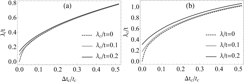
Figure 4: (a) The $\lambda$ values necessary to achieve a flat band with different fixed $\lambda_{c}$ values, after changing the $t_{c}=t_{c}^{rfbc}$ value defined by the rigid flat band conditions by $\Delta t_{c}$ (b) The $\lambda_{c}$ values necessary to achieve a flat band with different fixed $\lambda$ values, after changing the $t_{c}=t_{c}^{rfbc}$ value defined by the rigid flat band conditions by $\Delta t_{c}$. For exemplification we have used the Set.1 of Hamiltonian parameter data from Appendix D.

Figure 5: The $\lambda$, $\lambda_{c}$ values necessary to achieve a flat band after changing the $t_{c}=t_{c}^{rfbc}$ value defined by the rigid flat band conditions by $\Delta t_{c}$. The changed $\Delta t_{f}$ values were obtained by changing the $t_{h}$ hopping magnitude, therefore the value of $t_{h}$ is continuously changing along the solid lines, form the original $t_{h}$ to $1.5t_{h}$. In case a) one has $\lambda=constant$, while in the case b) $\lambda_{c}=constant$ holds. For exemplification we have used the Set.1 of Hamiltonian parameter data from Appendix D.

What one obtains is exemplified in Fig.4. The arbitrarily chosen Hamiltonian parameters, together with $t_{f}^{rfbc}$ and $t_{c}^{rfbc}$ are those used in Appendix D. One observes that even $50\%$ change in $t_{c}^{rfbc}$ can be easily compensated by $\lambda$ or $\lambda_{c}$ in reproducing the flat band in its initial position. One further observes that the in-base SOI ($\lambda$) is more efficient than its inter-base ($\lambda_{c}$) counterpart, since smaller $\lambda$ values are able to compensate the same $\Delta t_{c}$ values in reproducing the flat band. As seen, indeed the rigid flat band condition is substantially relaxed by SOI, at least at the level of $t_{c}$. The price of the re-flattened band to remain in the same position is that not all rigidly fixed Hamiltonian parameters can be relaxed (such as $t_{f}^{rfbc}$ in the present case). In such situation traditional procedures can be combined with SOI in order to achieve the re-flattening after the application of the $\Delta t_{c}\neq 0$ rigid flat band condition relaxation. In this case $\Delta t_{f}$ can be obtained by changing the side group connected to the pentagon [see Fig.2, where the side group $NH_{2}$ appears in the top (apical) part of the figure]. In the same time with this step, the counter apical (i.e. the N-N bond in Fig.2) hopping matrix element $t_{h}$ must be modified, which can be achieved e.g. by doping polyaminotriazole with $ClO_{4}$ ($PATClO_{4}$), fluorine ($PATF$), $HF_{2}$ ($PATHF_{2}$), etc. What is obtained is exemplified in Fig.5. We must here underline that higher $\lambda_{c}$ values allow higher $\Delta t_{f}$ values to be achieved in the attempt to transform the band back to a flat band. On this line we mention that by introducing heavy ions on intercell bonds we are able to increase the SOI coupling along the inter-base bonds E57 , and as seen here, this step would allow to increase the deviation from “rfbc” values in the process of band flattening.

Figure 6: The $\bar{\lambda}=\lambda=\lambda_{c}$ value necessary to compensate the deviation $\Delta t_{c}\neq 0$ from $t_{c}^{rfbc}$ in order to re-create the flat band at the origin of the energy axis. For exemplification we have used the Set.1 of Hamiltonian parameter data from Appendix D.

Often it happens that one has a pentagon polymer chain in which external side groups (apical atoms) are not present, doping is not used, and also heavy ion introductions on inter-base bonds is missing. In this case $\lambda=\lambda_{c}=\bar{\lambda}$ values can be tuned by external electric field as specified in Eq.(6). In such conditions, deviations $\Delta t_{c}\neq 0$ from $t_{c}^{rfbc}$ can be compensated by $\bar{\lambda}$ as shown in Fig.6 in order to create back the flat band at the origin of the energy axis.

IV.3 Relaxing the rigid flat band conditions by SOI at $B\neq 0$

When $B\neq 0$ holds, the flat band conditions Eq.(15) can be written as

$$\frac{1}{A_{f}}(-K_{g}v-S_{g}u)=0,\quad\frac{1}{A_{f}}(K_{g}u-S_{g}v)=0,$$ (20)

where the following notations have been introduced

$$K_{g}=\frac{\cos(4\varphi_{3}+\varphi_{b})}{\bar{\bar{\epsilon}}_{3}}-t_{h}\frac{\cos(2\varphi_{3})}{\bar{\epsilon}_{2}\bar{\bar{\epsilon}}_{2}},\quad S_{g}=\frac{\sin(4\varphi_{3}+\varphi_{b})}{\bar{\bar{\epsilon}}_{3}}-t_{h}\frac{\sin(2\varphi_{3})}{\bar{\epsilon}_{2}\bar{\bar{\epsilon}}_{2}},$$

$$v=2(2\lambda\lambda_{c}t+t_{c}(\lambda^{2}-t^{2})),\quad u=2(-2\lambda tt_{c}+\lambda_{c}(\lambda^{2}-t^{2})),$$

$$\varphi=\varphi_{b}+2\varphi_{3},\quad\varphi_{b}=\varphi_{1}+2\varphi_{2}.$$ (21)

Since for the Rashba interaction considered here $\lambda,\lambda_{c}$ must be real, Eq.(20) allows solutions only for $K_{g}=S_{g}=0$, which provide

$$I_{c}=I_{s}=I_{\varphi},\quad I_{\varphi}=X_{\varphi},$$

$$I_{c}=\frac{\cos(2\varphi_{3})}{\cos(4\varphi_{3}+\varphi_{b})},\quad I_{s}=\frac{\sin(2\varphi_{3})}{\sin(4\varphi_{3}+\varphi_{b})},\quad X_{\varphi}=\frac{\epsilon_{4}}{t_{h}}\frac{(\epsilon_{2}^{2}-t_{h}^{2})}{(\epsilon_{3}\epsilon_{4}-t_{f}^{2})}.$$ (22)

For solving Eq.(22) one studies the equality $I_{s}=I_{c}$. Before starting this job, let us underline that in the limit of zero external magnetic field, this equality gives $I_{\varphi}=X_{\varphi}=1$ and we reobtain the $B=0$ flat band condition deduced previously in Eq.(16). For $B\neq 0$, using $\sin(\alpha-\beta)=\sin(\alpha)\cos(\beta)-\cos(\alpha)\sin(\beta)$, the $I_{s}=I_{c}$ relation gives

$$\sin[(4\varphi_{3}+\varphi_{b})-2\varphi_{3}]=\sin(\varphi)=0,\quad i.e.\quad\varphi=\pm n\pi,$$ (23)

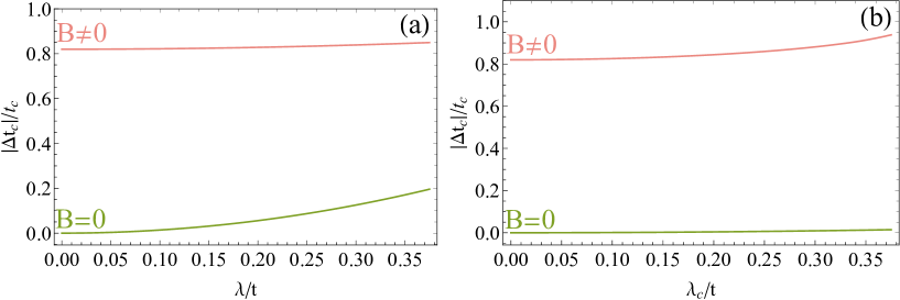
Figure 7: a) $\lambda$ and b) $\lambda_{c}$ spin orbit coupling values deduced at $B\neq 0$ (upper) and $B=0$ (lower) necessary to compensate the deviation $\Delta t_{c}\neq 0$ from $t_{c}^{rfbc}$ in order to re-create the flat band at the origin of the energy axis. For exemplification we have used the Set.2 of Hamiltonian parameter data from Appendix D.

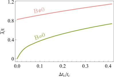
Figure 8: The $\bar{\lambda}=\lambda=\lambda_{c}$ spin orbit coupling values deduced at $B\neq 0$ (upper) and $B=0$ (lower) necessary to compensate the deviation $\Delta t_{c}\neq 0$ from $t_{c}^{rfbc}$ in order to re-create the flat band at the origin of the energy axis. For exemplification we have used the Set.3 of Hamiltonian parameter data from Appendix D.

where $n$ is an integer number or zero. Hence at $I_{s}=I_{c}$, one obtains $I_{s}=\sin(2\varphi_{3})/\sin(\pm n\pi+2\varphi_{3})$, consequently $I_{\varphi}=X_{\varphi}=\pm 1$, where the upper sign is obtained at $n=0$, while the lower sign at other $n$ values. One further observes that when Eq.(23) holds, Eq.(19) remains true, so the first line of Eq.(14) reduces to Eq.(19) when the flat band appears in the presence of the external magnetic field in the same position of the energy axis. Since $X_{\varphi}=1$, as mentioned above, reproduces the $B=0$ results (i.e. $\Delta t_{c}=\Delta t_{f}=0$ holds in this case), the $B\neq 0$ characteristics can be derived from the $X_{\varphi}=-1$ relation. Based on the last equality of the second line of Eq.(22), we obtain four different possible deviations $\Delta t_{f}$ from the $t_{f}^{rfbc}$ value, which are able to re-flatten the band at $B\neq 0$ in the same position of the energy axis in which it was placed the flat band at $B=0$:

$$\Delta t_{f}=\pm\frac{\sqrt{\epsilon_{4}[\epsilon_{3}t_{h}-(\epsilon_{2}^{2}-t_{h}^{2})]}}{\sqrt{t_{h}}}\pm\frac{\sqrt{\epsilon_{4}[\epsilon_{3}t_{h}+(\epsilon_{2}^{2}-t_{h}^{2})]}}{\sqrt{t_{h}}},$$ (24)

How $\Delta t_{c}$ modifies as function of the spin orbit coupling in flattening the band at $B\neq 0$ (placing the flat band in the same position of the energy axis in which the flat band for $t_{f}=t_{f}^{rfbc},t_{c}=t_{c}^{rfbc}$ was placed at $B=0$) is exemplified in Fig.7. The presented $|\Delta t_{c}|/t_{c}$ results were deduced from the $T_{0}$ expression of Eq.(14) in condition of Eq.(23). The $\bar{\lambda}=\lambda=\lambda_{c}$ results are similar, and are presented in Fig.8.

Based on the results presented in this subsection relating the $B\neq 0$ case, the following observations can be made: 1) It can be observed that only discrete nonzero external magnetic field values provide re-flattening effects [see Eq.(23)]. 2) As shown by Fig.7 and Eq.(24), huge $\Delta t_{c}/t_{c}$ and $\Delta t_{f}/t_{f}$ values can be achieved at $B\neq 0$ [allowed by the point 1)] in relaxing the rigid flat band conditions necessary for obtaining a flat band in the same position of the energy axis. Fig.7 shows that 80% deviations from $t_{c}^{rfbc}$ can be easily compensated by relatively small spin-orbit interaction values, and based on Eq.(24) it can be checked that 40-50% deviations from $t_{f}^{rfbc}$ can be achieved in producing a flat band at nonzero $B$. 3) The requirement to maintain a fixed flat band position on the energy axis is relatively restrictive since it does not allow all rigidly fixed flat band conditions to be continuously relaxed. In the present case, at $B\neq 0$, the $t_{f}^{rfbc}$ can be only discretely modified when flat bands are intended to be manufactured. 4) Since the condition in Eq.(23) is connected only to the total flux threading the unit cell, it results that in distorting the unit cell, new aspects in the band flattening via spin orbit interaction are not encountered.

V Relaxing the rigid flat band conditions without maintaining the position of the flat band

Let us consider that one has a flat band at $B=\lambda=\lambda_{c}=0$ which is placed in the origin of the energy axis, i.e. at $\epsilon=\epsilon_{1}=0$. As described previously, for the Hamiltonian parameters, this flat band emergence requires rigidly fixed flat band conditions, e.g. in the present case $t_{f}=t^{rfbc}_{f},t_{c}=t^{rfbc}_{c}$. Now we modify $t_{f}$ and $t_{c}$ with $\Delta t_{f}$ and $\Delta t_{c}$ relative to $t_{f}=t^{rfbc}_{f}$, and $t_{c}=t^{rfbc}_{c}$, the studied flat band becoming dispersive as exemplified in Appendix E. After this step we turn on the SOI such to transform back the dispersive band obtained in the previous step into a flat band placed in the position $\epsilon=\epsilon_{2}$. In the previous Section IV., we have analyzed the characteristics of this re-flattening process for $\epsilon_{1}=\epsilon_{2}=0$, i.e. for the case in which the re-flattened band emerges in the same position of the energy axis. Contrary to this, in the present Section V. we will analyze the case $\epsilon_{1}\neq\epsilon_{2}$, i.e. the situation in which the starting flat band position $\epsilon_{1}$ obtained at $t_{f}=t^{rfbc}_{f},t_{c}=t^{rfbc}_{c}$, and $B=\lambda=\lambda_{c}=0$, will be different from the position $\epsilon_{2}$ of the flat band obtained via SOI at the end of the process. As it will be seen from the results, this situation allows to considerably relax all rigidly fixed flat band conditions, hence allows to manufacture flat bands in real systems under easier conditions.

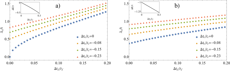
Figure 9: The $\lambda_{c}$ spin orbit coupling values necessary to compensate at $\lambda=0$ the common deviations $\Delta t_{c}\neq 0$ and $\Delta t_{f}\neq 0$ at a) $B=0$, and b) $B\neq 0$, in order to re-create a flat band placed originally (at $\lambda=\lambda_{c}=B=0$) in the origin of the energy axis $\epsilon=0$. The new position of the flat band is at $\epsilon=\Delta E$. In this figure $\Delta t_{c}/t_{c}<0$ holds. For exemplification we have used the Set.4 of Hamiltonian parameter data from Appendix D.

Figure 10: The $\lambda_{c}$ spin orbit coupling values necessary to compensate at $\lambda=0$ the common deviations $\Delta t_{c}\neq 0$ and $\Delta t_{f}\neq 0$ at a) $B=0$, and b) $B\neq 0$ in order to re-create a flat band placed originally (at $\lambda=\lambda_{c}=B=0$) in the origin of the energy axis $\epsilon=0$. The new position of the flat band is at $\epsilon=\Delta E$. In this figure $\Delta t_{c}/t_{c}>0$ holds. For exemplification we have used the Set.4 of Hamiltonian parameter data from Appendix D.

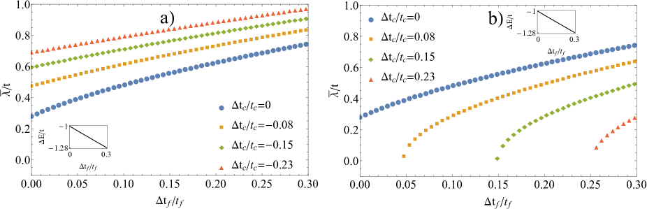
Figure 11: The $\lambda_{c}=\lambda=\bar{\lambda}$ spin orbit coupling values necessary to compensate the common deviations $\Delta t_{c}\neq 0$ and $\Delta t_{f}\neq 0$ at $B\neq 0$ and a) $\Delta t_{c}/t_{c}<0$, and b) $\Delta t_{c}/t_{c}>0$, in order to re-create a flat band placed originally (at $\bar{\lambda}=B=0$) at the origin of the energy axis $\epsilon=0$. The new position of the flat band is at $\epsilon=\Delta E$. For exemplification we have used the Set.4 of Hamiltonian parameter data from Appendix D.

Fig.9 (at $\Delta t_{c}/t_{c}<0$) and Fig.10 (at $\Delta t_{c}/t_{c}>0$) exemplifies the obtained results at $\lambda=0$. In these figures, the a) plots show the $B=0$ case, while the b) plots the $B\neq 0$ situation. It can be seen that even 20 $\%$ modification of $t_{c}^{rfbc}$ or $t_{f}^{rfbc}$ can be compensated by the presence of $\lambda_{c}$ in reproducing the flat band in a shifted position $\Delta E$ presented in the inset. It can be observed that all rigidly fixed Hamiltonian parameters can be relaxed in this case. In the presence of the external magnetic field $B$ larger $\Delta t_{f}/t_{f}$ deviations can be compensated by smaller $\lambda_{c}$ values, which underlines the importance of the consideration of $B$ in this process. In this case $\lambda_{c}$ can be modified by atom intercalation in the intercell bonds, structural conformation or twist application E51 ; E53 ; E54a ; E54b .

When one considers the intrinsic $\lambda$ and $\lambda_{c}$ small, and we tune both of them by external electric field, the $\lambda=\lambda_{c}=\bar{\lambda}$ case must be considered presented in Fig.11 which is plotted at nonzero and constant $B$. It can be observed that e.g. almost 30 $\%$ positive displacements in $\Delta t_{c}/t_{c}$ and $\Delta t_{f}/t_{f}$ can be compensated by relatively small $\bar{\lambda}/t$ values of order $10^{-2}$.

VI Further remarks

Several observations and remarks we would like to add in what will follows.

a) We approach the presented subject in fact in a mathematical language since this allows to show how the flat bands can be detected in general terms in an arbitrary case, how the flat band conditions can be deduced in a general case, shows that a part of the flat band conditions enumerated in the literature in fact provide the position of the flat band on the energy scale.

b) We have used different input parameters in Table I-II presented in Appendix D in order to underline that our findings, observations and technical approach to the problem are not related only to one given material, but have an extremely broad application spectrum. The used Hamiltonian parameters are not new, have not been introduced in this paper, all of them have a broad literature. Consequently, how these parameters affect the band structure is known. For example, in the case of conducting polymers, how the hopping parameters ($t_{i}$) and on-site one particle potentials ($\epsilon_{i}$) influence the band structure is seen e.g. in E18 ; E20 ; EX1 ; EX2 etc. How the Peierls phase factors – describing the action of the external magnetic field on the orbital motion of itinerant electrons – acts on the band structure is seen e.g. in E21 ; EX3 ; EX4 etc. How the many-body spin-orbit interaction acts on the band structure (in most cases the main effect is that breaks the spin projection double degeneracy of each band), is seen e.g. in E38 ; E39 ; EX5 ; EX6 , etc. This is why in this paper we concentrate on a single band not satisfying, but being in the absence of spin-orbit interaction closely placed to the rigid flat band conditions.

c) In order to exemplify inside the whole band structure the many-body SOI flattening effect we present Fig.12, where the polyaminotriazole case is exemplified in zero external magnetic field. The used Hamiltonian parameters are $t_{f}/t=1$ (see Ref.E18 ; EX1 ), and $t_{h}/t=0.93,t_{c}/t=1.06,\epsilon_{1}/t=\epsilon_{2}/t=0.33,\epsilon_{3}/t=1.66,\epsilon_{4}/t=0.8$, see Ref.EX7 . The rigid flat band conditions require in the absence of external fields and $\lambda=\lambda_{c}=0$ the values $t_{f}^{rfbc}=1.406$, $t_{c}^{rfbc}=1.996$ (in $t$ units). As seen, $\lambda/t=0.17$ provides $\Delta t_{f}/t_{f}=0.40$, $\Delta t_{c}/t_{c}=0.88$ relaxation of rigid flat band conditions.

Figure 12: The many-body spin-orbit interaction effect on the whole band structure: a) the $\lambda=\lambda_{c}=B=0$ case providing dispersive bands, and b) at $B=0$ the $\lambda/t=0.178$ providing a double degenerate flat band (see Appendix C). For the Hamiltonian parameters see text.

In the presented case, the flat band emerges at the position of the third band (see Fig.12.a). One notes, that in general, sign changes in the Hamiltonian parameters change the position of the resulting flat band.

d) Concerning the contribution of terms not taken into account in the Hamiltonian presented in Eq.(3) the following aspects must be underlined: First, as mentioned previously in the text following Eq.(5), in the used configuration the Zeeman term provides zero contribution because when the external magnetic field ${\bf B}$ is applied, the carrier spin is perpendicular to the magnetic field, hence the scalar product ${\bf B}\cdot{\bf\sigma}=0$ holds. Second, if electric dipole moment ${\bf p}$ is present, it provides a supplementary contribution to the applied external electric field. In the case of the described conducting polymers, the dipole moment vector (if exists) is placed inside the plane x0y of the polymer. The dipole moment itself originates usually from the inside of the unit cell, being relatively small, as order of magnitude around or below 1 debye EX8 . Our analyzed external electric field ${\bf E}$ is perpendicular to the plane of the polymer, so ${\bf E}\cdot{\bf p}=0$, consequently the Stark contribution is also missing from the Hamiltonian.

But it must be mentioned, that in special cases, in order to enhance special applications (e.g. in energy storage, or solar cell manufacturing), it is possible to attach to the polymer EX9 group of atoms with high dipole moment, even oriented outside of the polymer plane. In such cases the presented results and findings remain true, but the external electric field is additively renormalized by the electric field created by the dipole moments.

e) If we concentrate on the question why the flat bands emerge, the answer to this question underlined in this paper is as follows: The band structure is given by the secular equation [Q=0, see Eq.(1)] of the one particle part of the Hamiltonian transformed in the k-space. As explained, always

$$Q=T_{0}+\sum_{j=1}^{m}T_{j}\>trig_{j}({\bf k}{\bf x}_{\alpha}),$$ (25)

where ${\bf x}_{\alpha}$ are the Bravais vectors, ${\bf k}$ the momentum, and the prefactors $T_{0},T_{1},...T_{m}$ depend only on the Hamiltonian parameters $\{p_{i}\}$ and the energy $\epsilon$. The bands are given by $\epsilon=E_{n}({\bf k})$ solutions of the $Q=0$ secular equations. Flat bands are obtained always when all $T_{j}=0$, see Eq.(2), hence $\epsilon$ becomes ${\bf k}$ independent (and the flat band position will be given by the $T_{0}=0$ relation). This is the mathematical origin of the flat bands. How we achieve the all $T_{j}=0$ requirements ? We simply tune the Hamiltonian parameters $\{p_{i}\}$. We underline that the here described procedure can be applied always. It also means that flat bands are not the privilege of some special systems, since flat bands can be obtained from each system by a proper tuning of the Hamiltonian parameters, procedure which is effectively often used (see e.g. Refs. EX10 ; EX11 ). E.g. for a simple cubic lattice in a simple tight binding approximation, from Q=0 one obtains for the lowest band the relation $\epsilon-A_{0}-A_{1}[cos(xk_{x})+cos(yk_{y})+cos(zk_{z})]=0$, where $T_{0}=\epsilon-A_{0},T_{1}=A_{1}\sim t$ holds, $t$ being the nearest neighbor hopping integral. The $T_{1}=A_{1}=0$ condition provides a flat band at the position $\epsilon=A_{0}$.

Now if we ask: what it happens physically when all $T_{j}=0$ relations hold, the answer to this question varies from case to case. For example, in the simple cubic lattice case exemplified above, $A_{1}=0$ occurs when the nearest-neighbor overlap becomes zero (e.g. when we increase the lattice constant at fixed itinerant carrier number, i.e. decrease the carrier concentration), and we reach a low concentration insulating localized state, (e.g. Wigner lattice, since the Coulomb repulsion is always present). The problem becomes complicated also because there are flat bands with itinerant (i.e. non-localized) carriers (see e.g. Ref. E13 ). In the situation when carriers are localized in the flat band, often the all $T_{j}=0$ relations are considered related to destructive interference caused by frustration, or lattice geometry (see e.g. Refs. EX10 ; EX11 ). In the conducting polymer case exemplified in this paper, one knows that in the flat band, the one-particle Wannier states are extended over two cells but are localized (see e.g. Fig.1 of Ref. EX1 ). These Wannier states can be expressed as a linear combination of extended Bloch states. Hence, in explaining the two cell extension of the Wannier states, the destructive interference argument can be invoked also here.

It is important to stress, that independent on how we interpret physically Eq.(2), i.e. the all $T_{j}=0$ relations, the here described procedure in deducing the flat band emergence always works.

VII Summary and conclusions

One knows that in a real system, the emergence of a flat band is connected to rigid mathematical conditions (i.e. flat band conditions) relating a part of the Hamiltonian parameters (which we denote here by $\xi_{i}$, e.g. in the presented paper, $\xi_{1}=t_{c},\xi_{2}=t_{f}$). Because of these rigid and restrictive conditions, the engineering of a flat band in a real system is a quite difficult task. Indeed, for this to be possible, the rigidly fixed Hamiltonian parameters must be tuned exactly to the values fixed by the flat band conditions in order to obtain a flat band in the system. From the other side, given by their high (practically infinitely large) degeneracy, there is a huge need for flat bands in different systems, because introducing a small perturbation in such case, the ground state of such materials can be easily pushed in the direction of several ordered phases of interest in different applications. Because of these reasons, the study of procedures that are able to relax the rigid flat band conditions is an important task.

On this line, in this paper we demonstrate, that the many-body spin-orbit interaction (SOI) is able to substantially relax the rigid flat band conditions, and at the same time can be continuously tuned by external fields. Consequently taking SOI into account, the flat band manufacturing in real systems becomes an easier task.

The problem detailed above is analyzed in the case of conducting polymers. Besides the broad application possibilities of these materials, the motivation of this choice is the fact that the mathematical background of the flat band conditions can be presented in this case in full generality but in a clear, visible and understandable manner. One even has the possibility to analyze the action of in-cell ($\lambda$), and inter-cell ($\lambda_{c}$) SOI contributions separately. The procedure we use is simple: first, fixing the position of the flat band at the origin of the energy axis $\epsilon=0$, we deduce the flat band conditions at zero external fields and zero SOI. Then, for a fixed set of Hamiltonian parameters that can be arbitrarily chosen, we deduce the rigidly fixed values of Hamiltonian parameters $\xi_{i}=\xi_{i}^{rfbc}$. After this step we destroy the flat band (transforming it into a dispersive band) by modifying $\xi_{i}$ from $\xi_{i}^{rfbc}$ to $\xi_{i}^{\prime}=\xi_{i}^{rfbc}+\Delta\xi_{i}$, and analyze what SOI values transform the dispersive band back into a flat band placed in the position $\epsilon^{\prime}$. In this manner, at the appearance of the flat band, the parameters $\xi_{i}$ are no more rigidly fixed to $\xi_{i}^{rfbc}$, but take the values $\xi_{i}^{\prime}$, hence are relaxed by $\Delta\xi_{i}=\xi_{i}^{\prime}-\xi_{i}^{rfbc}$.

In the first step we analyze the case $\epsilon=\epsilon^{\prime}$, so the destroyed flat band, after the application of SOI arrives back in its original position. This situation is usually considered in the literature, and is in fact restrictive since it does not allow to relax all rigidly fixed flat band conditions. The relaxed parameters however, calculated as $\Delta\xi_{i}/\xi_{i}$, can be easily changed by $20-30\%$ relative to their initial value. The application of an external $B$ magnetic field increases (at fixed SOI) the possible $\Delta\xi_{i}/\xi_{i}$ values even to 80 $\%$ (see e.g. Fig.7). Comparing to the case mentioned above, as a novelty, we also analyze the case $\epsilon^{\prime}\neq\epsilon$ in the second step. In this situation, in fact, mathematically, one of the flat band conditions is missing, so the rigid flat band conditions are not so restrictive. In this case, the relative flat band position displacement on an arbitrary scale $|\Delta\epsilon/\epsilon|$ is relatively small (i.e. 10-20 $\%$), and contrary to the first case, all rigidly fixed Hamilton operator parameters $\xi_{i}^{rfbc}$ can be relaxed by 20-30 $\%$ with relatively small SOI coupling values (see e.g. Fig.11.b, where even $\lambda/t<0.1$). Also in this case, the presence of the external magnetic field enhances the relaxation process of the rigidly fixed Hamiltonian parameter values.

Concerning the question: how can the SOI couplings be modified and tuned, several possibilities exist. One has discrete tuning possibilities, as for example intercalation of elements with high spin-orbit coupling on bonds connecting cells (e.g. intrachain heavy atoms), hence modifying $\lambda_{c}$. But more promising possibilities are provided by continuous modification possibilities as for example via torsioning, twisting, or application of external electric field. From these, the last possibility seems to be the most attractive (from the data published in the literature, see e.g. [E54 ], $\lambda\sim 0.02$ eV is attained usually by electric fields of order $E\sim$ kV/cm).

We strongly hope that the presented results will considerably enhance the flat band engineering of real materials.

VIII Bibliography

Appendix A The Peierls phase factors

In calculating the $\varphi_{ji}$ Peierls phase factors, one follows Fig.1. In the presence of the external magnetic field $B\neq 0$ they modify the hopping matrix elements according to the relation

$$t_{j\leftarrow i}(B)=t_{j\leftarrow i}(0)e^{i\frac{2\pi}{\phi_{0}}\int_{i}^{j}\vec{A}\vec{dl}}=t_{j\leftarrow i}(0)e^{i\varphi_{ji}},$$ (26)

where $\phi_{0}=\frac{hc}{e}$ is the flux quantum. One has $\varphi_{ji}=\frac{2\pi}{\phi_{0}}\int_{i}^{j}\vec{A}\vec{dl}$, and $t_{j\leftarrow i}(0)$ are the $B=0$ hopping matrix elements. Since $B=rot(\vec{A})$ holds, and $B$ points to the $z$ direction, we use the gauge $A_{x}=-By,A_{y}=A_{z}=0$. After this step all exact $\varphi_{ji}$ Peierls phase factors can be calculated for each bond. One observes that $\varphi_{56}=0$, since the scalar product is zero ($\vec{A}\perp\vec{dl}$), and $\varphi_{47}$ is also $0$, because $y=0$ holds (see Fig.1). One obtains

$$\varphi_{3\leftarrow 2}=\frac{2\pi}{\phi_{0}}(-By_{2}),\varphi_{3\leftarrow 2}=\varphi_{1},$$

$$\varphi_{4\leftarrow 3}=\frac{2\pi B}{\phi_{0}}\frac{|y_{2}|b_{2}}{2},\varphi_{2\leftarrow 1}=\varphi_{4\leftarrow 3}=\varphi_{2},$$

$$\varphi_{5\leftarrow 4}=\frac{2\pi}{\phi_{0}}B\frac{y_{1}b}{4},\quad\varphi_{5\leftarrow 4}=\varphi_{1\leftarrow 5}=\varphi_{3}.$$ (27)

One further has

$$\varphi=\varphi_{1}+2\varphi_{2}+2\varphi_{3}=\frac{2\pi}{\phi_{0}}\phi,$$ (28)

where $\phi=BS$, represents the flux trough the unit cell, $S=|y_{2}|b_{1}+2\frac{|y_{2}|b_{2}}{2}+2\frac{y_{1}b}{4}$.

Taking these results into account, the following hopping terms are present in the Hamiltonian:

$$t_{32}^{\uparrow,\uparrow}=t_{h}e^{i\varphi_{1}},\varphi_{1}=\frac{2\pi}{\phi_{0}}(-By_{2})$$

$$t_{21}^{\uparrow,\uparrow}=te^{i\varphi_{2}},t_{43}^{\uparrow,\uparrow}=te^{i\varphi_{2}},t_{21}^{\uparrow,\downarrow}=\lambda e^{i\varphi_{2}},t_{43}^{\uparrow,\downarrow}=\lambda e^{i\varphi_{2}},\varphi_{2}=\frac{2\pi}{\phi_{0}}B\frac{|y_{2}|b_{2}}{2},$$

$$t_{54}^{\uparrow,\uparrow}=te^{i\varphi_{3}},t_{15}=te^{i\varphi_{3}},t_{54}^{\uparrow,\downarrow}=-\lambda e^{i\varphi_{3}},t_{15}^{\uparrow,\downarrow}=-\lambda e^{i\varphi_{3}},\varphi_{3}=\frac{2\pi}{\phi_{0}}B\frac{y_{1}b}{4},$$ (29)

while $t_{i,j}^{\uparrow,\uparrow}=t_{i,j}^{\downarrow,\downarrow}$, $t_{i,j}^{\uparrow,\downarrow}=-t_{i,j}^{\downarrow,\uparrow}$ holds, since we have taken only Rashba spin-orbit interactions into account E54 .

Appendix B The secular equation

The Secular equation Eq.(11) in which Eq.(10) has been introduced can be mathematically reduced to the diagonalization of the following $4\times 4$ matrix:

$$\begin{pmatrix}A_{f}&e^{-ikb}(t_{c}e^{ika}-W_{1})&0&e^{-ikb}(\lambda_{c}e^{ika}-W_{2})\\ e^{ikb}(t_{c}e^{-ika}-W_{1}^{*})&A_{f}&e^{ikb}(-\lambda_{c}e^{-ika}+W_{2}^{*})&0\\ 0&e^{-ikb}(-\lambda_{c}e^{ika}+W_{2})&A_{f}&e^{-ikb}(t_{c}e^{ika}-W_{1})\\ e^{ikb}(\lambda_{c}e^{-ika}-W_{2}^{*})&0&e^{ikb}(t_{c}e^{-ika}-W_{1}^{*})&A_{f}\end{pmatrix},$$ (30)

where $W_{1f}=(\lambda^{2}-t^{2})\left(\frac{1}{\bar{\epsilon}_{2}\bar{\bar{\epsilon}}_{2}}t_{h}e^{-i\varphi}-\frac{1}{\bar{\bar{\epsilon}}_{3}}\right)$, $W_{2f}=2\lambda t\left(\frac{1}{\bar{\epsilon}_{2}\bar{\bar{\epsilon}}_{2}}t_{h}e^{-i\varphi}-\frac{1}{\bar{\bar{\epsilon}}_{3}}\right)$.

Furthermore the $A$ and $V$ expressions present in Eq.(12) are defined as:

$$A=A_{f} - \frac{1}{A_{f}}\left(\lambda_{c}e^{i(\varphi_{k}-2\varphi_{3})}+2\lambda t\xi\right)\left(\lambda_{c}e^{-i(\varphi_{k}-2\varphi_{3})}+2\lambda t\xi^{*}\right)$$ (31)

$$- \frac{1}{A_{f}}\left(t_{c}e^{i(\varphi_{k}-2\varphi_{3})}-(t^{2}-\lambda^{2})\xi\right)\left(t_{c}e^{-i(\varphi_{k}-2\varphi_{3})}-(t^{2}-\lambda^{2})\xi^{*}\right),$$

where

$$\xi=\left(\frac{\bar{\epsilon}_{4}}{\bar{\epsilon}_{3}\bar{\epsilon}_{4}-t_{f}^{2}}e^{i\varphi}-\frac{t_{h}}{\bar{\epsilon}_{2}^{2}-t_{h}^{2}}\right)$$ (32)

and

$$V= - \frac{1}{A_{f}}\left(\lambda_{c}e^{i(\varphi_{k}-2\varphi_{3})}+2\lambda t\xi\right)\left(t_{c}e^{-i(\varphi_{k}-2\varphi_{3})}-(t^{2}-\lambda^{2})\xi^{*}\right)-$$ (33)

$$- \frac{1}{A_{f}}\left(-\lambda_{c}e^{-i(\varphi_{k}-2\varphi_{3})}-2\lambda t\xi^{*}\right)\left(t_{c}e^{i(\varphi_{k}-2\varphi_{3})}-(t^{2}-\lambda^{2})\xi\right).$$

Appendix C The flat band conditions derived from the $(A-iV)$ expression

The studied expression can be written as:

$$(A-iV)=T_{0}+\bar{T}_{1}\cos(\varphi_{k})+\bar{T}_{2}\sin(\varphi_{k})=0,$$ (34)

where $T_{0}$ is the same as seen in (14), and $\bar{T}_{1},\bar{T}_{2}$ are given by

$$\bar{T}_{1}=\frac{1}{A_{f}}\bigg{(}-\cos(7\varphi_{3})\frac{2(2\lambda t\lambda_{c}+t_{c}(\lambda^{2}-t^{2}))}{\bar{\bar{\epsilon}}_{3}}+\sin(7\varphi_{3})\frac{2(-2\lambda tt_{c}+\lambda_{c}(\lambda^{2}-t^{2}))}{\bar{\bar{\epsilon}}_{3}}+$$

$$\hskip 14.22636pt+\cos(2\varphi_{3})\frac{2(2\lambda t\lambda_{c}+t_{c}(\lambda^{2}-t^{2}))t_{h}}{\bar{\epsilon}_{2}\bar{\bar{\epsilon}}_{2}}-\sin(2\varphi_{3})\frac{2(-2\lambda tt_{c}+\lambda_{c}(\lambda^{2}-t^{2}))t_{h}}{\bar{\epsilon}_{2}\bar{\bar{\epsilon}}_{2}}\bigg{)}=0,$$

$$\bar{T}_{2}=\frac{1}{A_{f}}\bigg{(}-\cos(7\varphi_{3})\frac{2(-2\lambda tt_{c}+\lambda_{c}(\lambda^{2}-t^{2}))}{\bar{\bar{\epsilon}}_{3}}-\sin(7\varphi_{3})\frac{2(2\lambda t\lambda_{c}+t_{c}(\lambda^{2}-t^{2}))}{\bar{\bar{\epsilon}}_{3}}+$$

$$\hskip 14.22636pt+\cos(2\varphi_{3})\frac{2(-2\lambda tt_{c}+\lambda_{c}(\lambda^{2}-t^{2}))t_{h}}{\bar{\epsilon}_{2}\bar{\bar{\epsilon}}_{2}}+\sin(2\varphi_{3})\frac{2(2\lambda t\lambda_{c}+t_{c}(\lambda^{2}-t^{2}))t_{h}}{\bar{\epsilon}_{2}\bar{\bar{\epsilon}}_{2}}\bigg{)}=0.$$ (35)

Using the same notation as in Eq.(20) this expression provides:

$$\bar{T}_{1}=\frac{1}{A_{f}}(-K_{g}v+S_{g}u)=0,\quad\bar{T}_{2}=\frac{1}{A_{f}}(-K_{g}u-S_{g}v)=0.$$ (36)

As in the case of Eq.(20), only the solution $K_{g}=S_{g}=0$ exists, hence we reobtain the solutions derived from the $(A+iV)$ expression. This is an important result because of the following reason: it is known that usually, the many-body spin orbit interaction breaks the spin-projection double degeneracy of each band E38 ; E41 . But here one observes, that if one creates a flat band using SOI, the flat band will remain double degenerated.

Appendix D Sets of Hamiltonian parameter data.

Set.1									Set.2
The unrestricted parameters						The parameters calculated from the flat band conditions			The unrestricted parameters						The parameters calculated from the flat band conditions
$\epsilon_{1}$	$\epsilon_{2}$	$\epsilon_{3}$	$\epsilon_{4}$	$t$	$t_{h}$	$t_{c}^{rfbc}$	$t_{f}^{rfbc}$		$\epsilon_{1}$	$\epsilon_{2}$	$\epsilon_{3}$	$\epsilon_{4}$	$t$	$t_{h}$	$t_{c}^{rfbc}$	$t_{f}^{rfbc}$
0.17	0.49	0.22	3.36	1	1.5	1.16	2.29		0.87	1.22	0.82	0.36	1	0.9	2.21	0.14

Table 1: The Set.1 and Set.2 of Hamiltonian parameter data.

Set.3									Set.4
The unrestricted parameters						The parameters calculated from the flat band conditions			The unrestricted parameters						The parameters calculated from the flat band conditions
$\epsilon_{1}$	$\epsilon_{2}$	$\epsilon_{3}$	$\epsilon_{4}$	$t$	$t_{h}$	$t_{c}^{rfbc}$	$t_{f}^{rfbc}$		$\epsilon_{1}$	$\epsilon_{2}$	$\epsilon_{3}$	$\epsilon_{4}$	$t$	$t_{h}$	$t_{c}^{rfbc}$	$t_{f}^{rfbc}$
0.11	0.10	0.92	0.86	1	0.85	1.44	1.23		0.65	0.49	1.4	0.86	1	2	1.31	1.68

Table 2: The Set.3 and Set.4 of Hamiltonian parameter data.

We note that in the Sets 1-4 all parameters presented are given in $t$ units, and the rigidly fixed flat band conditions have been deduced at $B=\lambda=\lambda_{c}=0$. In the cases of the Sets 2 and 4, when $B\neq 0$ plots are done, the $B$ value was deduced from Eq.(22), i.e. $I_{\varphi}=X_{\varphi}=-1$. E.g., for $\varphi_{b}=3\varphi_{3}$ (regular pentagon), one has at minimum $B$ the relation $\varphi_{3}=(1/5)\pi$. For connection to $B$, see also Eq.(A4).

Appendix E Dispersive bands from flat bands

Let us consider that at $B=\lambda=\lambda_{c}=0$ one modifies the $t_{c}=t_{c}^{rfbc}$ rigid flat band condition value. What happens to the band is exemplified in Fig.13, where $8.62\%$ modification has been taken into account relative to $t_{c}^{rfbc}$. As seen, the flat band becomes a dispersive band.

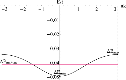
Figure 13: The flat band originally placed at the origin of the energy axis, becomes dispersive under the action of $\Delta t_{c}$ at zero SOI couplings. The line in the middle of the dispersive band (at position $\Delta\bar{E}_{median}$) shows the median of the band, while $\Delta\bar{E}_{min}$ and $\Delta\bar{E}_{max}$ denote the minimum and maximum position in the dispersive band relative to the median. The $\Delta\bar{E}_{\alpha}$, $\alpha=median,min,max$ values are indicated in $t$ units. For exemplification we have used the Set 1. of Hamiltonian parameter data from Appendix D.

How $\Delta\bar{E}_{median}$, $\Delta\bar{E}_{min}$ and $\Delta\bar{E}_{max}$ change as function of $\Delta t_{c}$ is exemplified in Fig.14.

Figure 14: The different $\Delta\bar{E}_{\alpha}$ quantities from Fig.12 as function of $\Delta t_{c}$ normalized to $t_{c}=t_{c}^{rfbc}$. The presented cases: (a) the median- ($\Delta\bar{E}_{median}$), (b) the maximum- ($\Delta\bar{E}_{max}$), and (c) the minimum ($\Delta\bar{E}_{min}$). For exemplification we have used the Set 1. of Hamiltonian parameter data from Appendix D.

One notes that the original flat band placed in the origin of the energy axis was double degenerated relative to the spin projection, and since $\lambda=\lambda_{c}=0$, this double degeneracy remains valid also in the case of the dispersive band emerging at $\Delta t_{c}\neq 0$.

References

- (1) L. Yu, H. Xue, B. Zhang, Topological slow light via coupling chiral edge modes with flat bands, Appl. Phys. Lett. 118, 071102 (2021). https://doi.org/10.1063/5.0039839
- (2) Y. He, R. Mao, H. Cai, J.-X. Zhang, Y. Li, L. Yuan, S.-Y. Zhu, D.-W. Wang, Flat-band localization in Creutz superradiance lattices, Phys. Rev. Lett. 126, 103601 (2021). https://doi.org/10.1103/PhysRevLett.126.103601
- (3) T.-H. Leung, M. N. Schwarz, S.-W. Chang, C. D. Brown, G. Unnikrishnan, D. Stamper-Kurn, Interaction-Enhanced Group Velocity of Bosons in the Flat Band of an Optical Kagome Lattice, Phys. Rev. Lett. 125, 133001 (2020). https://doi.org/10.1103/PhysRevLett.125.133001
- (4) G. Caceres-Aravena, L. E. F. Foa, R. A. Vicencio, Topological and flat bands states induced by hybridized interactions in one-dimensional photonic lattices, Phys. Rev. A 102, 023505 (2020). https://doi.org/10.1103/PhysRevA.102.023505
- (5) S. M. Zhang, L. Jin, Flat band in two-dimensional non-Hermitian optical lattices, Phys. Rev. A 100, 043808 (2019). https://doi.org/10.1103/PhysRevA.100.043808
- (6) M. Milićević, G. Montambaux, T. Ozawa, I. Sagnes, A. Lemaître, L. Le Gratiet, A. Harouri, J. Bloch, A. Amo, Type-III and Tilted Dirac Cones emerging from flat bands in photonic orbital graphene, Phys. Rev. X 9, 031010 (2019). https://doi.org/10.1103/PhysRevX.9.031010
- (7) N. Lazarides, G. P. Tsironis, Compact Localized States in Engineered Flat-Band PT Metamaterials, Sci Rep 9, 4904 (2019). https://doi.org/10.1038/s41598-019-41155-8
- (8) J.-W. Rhim, B.-J. Yang, Singular flat bands, arXiv:2012.04279 https://arxiv.org/abs/2012.04279
- (9) D. Leykam, A. Andreanov, S. Flach, Artificial flat band systems: from lattice models to experiments, Adv. Phys.: X 3, 1473052 (2018). https://doi.org/10.1080/23746149.2018.1473052
- (10) N. Lazarides, G. P. Tsironis, SQUID Metamaterials on a Lieb lattice: From flat-band to nonlinear localization, Phys. Rev. B 96, 054305 (2017). https://doi.org/10.1103/PhysRevB.96.054305
- (11) G. Hu, Q. Ou, G. Si et al., Topological polaritons and photonic magic angles in twisted -MoO3 bilayers. Nature 582, 209–213 (2020). https://doi.org/10.1038/s41586-020-2359-9
- (12) A. Mielke, H. Tasaki, Ferromagnetism in the Hubbard model, Commun.Math. Phys. 158, 341–371 (1993). https://doi.org/10.1007/BF02108079
- (13) Z. Gulacsi, A. Kampf, D. Vollhardt, Route to ferromagnetism in organic polimers, Phys. Rev. Lett. 105, 266403.1-266403.4 (2010). https://link.aps.org/doi/10.1103/PhysRevLett.105.266403.
- (14) R. M. Geilhufe, B. Olsthoorn, Identification of strongly interacting organic semimetals, Phys. Rev. B 102, 205134 (2020). https://link.aps.org/doi/10.1103/PhysRevB.102.205134
- (15) Z. Ni, B. Xu, M. A. Sanchez-Martinez, Y. Zhang, K. Manna, C. Bernhard, J. W. F. Venderbos, F. de Juan, C. Felser, A. G. Grushin, L. Wu, Linear and nonlinear optical responses in the chiral multifold semimetal RhSi, Quantum Materials 5, 96 (2020). https://doi.org/10.1038/s41535-020-00298-y
- (16) H. Guo, X. Zhang, G. Lu, Shedding Light on Moire Excitons: A First-Principles Perspective, Science Advances 6, eabc5638 (2020). https://doi.org/10.1126/sciadv.abc5638
- (17) W. Yan, H. Zhong, D. Song, Y. Zhang, S. Xia, L. Tang, D. Leykam, Z. Chen, Flatband Line States in Photonic Super-Honeycomb Lattices, Adv. Optical Mater. 8, 1902174 (2020). https://doi.org/10.1002/adom.201902174
- (18) Y. Suwa, R. Arita, K. Kuroki, H. Aoki, Flat-band ferromagnetism in organic polymers designed by a computer simulation, Phys. Rev. B 68, 174419 (2003). https://link.aps.org/doi/10.1103/PhysRevB.68.174419
- (19) Z. Gulácsi, A. Kampf, D. Vollhardt, Exact many-electron ground states on diamond and triangle Hubbard chains, Progress of Theoretical Physics Supplement 176, 1-21 (2008). https://doi.org/10.1143/PTPS.176.1
- (20) Z. Gulácsi, Exact ground states of correlated electrons on pentagon chains, Int. Jour. Mod. Phys. B 27, 1330009 (2013). https://doi.org/10.1142/S0217979213300090
- (21) Z. Gulácsi, A. Kampf, D. Vollhardt, Exact many-electron ground states on the diamond Hubbard chain, Phys. Rev. Lett. 99, 026404 (2007). https://link.aps.org/doi/10.1103/PhysRevLett.99.026404
- (22) R. Trencsényi, E. Kovács, Z. Gulácsi, Correlation and confinement induced itinerant ferromagnetism in chain structures, Phil. Mag. 89, 1953-1974 (2009). https://doi.org/10.1080/14786430902810498
- (23) S. Colonna, D. Battegazzore, M. Eleuteri, R. Arrigo, A. Fina, Properties of graphene-related materials controlling thermal conductivity of their polymer nanocomposites, Nanomaterials 10, 2167 (2020). https://doi.org/10.3390/nano10112167
- (24) D. Babajanov, H. Matyoqubov, D. Matrasulov, Charged solitons in branched conducting polymers, J. Chem. Phys. 149, 164908 (2018). https://doi.org/10.1063/1.5052044
- (25) T. Zhang, X. Wu, T. Luo, Polymer Nanofibers with Outstanding Thermal Conductivity and Thermal Stability: Fundamental Linkage between Molecular Characteristics and Macroscopic Thermal Properties, J. Phys. Chem. C 118, 21148-21159 (2014). https://doi.org/10.1021/jp5051639
- (26) J. F. Gu, S. Gorgutsa, M. Skorobogatiy, Soft capacitor fibers using conductive polymers for electronic textiles, Smart Mater. Struct. 19, 115006 (2010). http://dx.doi.org/10.1088/0964-1726/19/11/115006
- (27) J. Ratzsch, J. Karst, J. Fu, M. Ubl et al., Electrically switchable metasurface for beam steering using PEDOT, J. Opt. 22, 124001 (2020). http://dx.doi.org/10.1088/2040-8986/abc6fa
- (28) C. Harito, L. Utari, B. R. Putra, B. Yuliarto et al., The Development of Wearable Polymer-Based Sensors: Perspectives, J. Electrochem. Soc. 167, 037566 (2020). http://dx.doi.org/10.1149/1945-7111/ab697c
- (29) P. Sutton, P. Bennington, S. N. Patel, M. Stefik et al., Surface Reconstruction Limited Conductivity in Block-Copolymer Li Battery Electrolytes, Adv. Funct. Mater. 29, 1905977 (2019). https://doi.org/10.1002/adfm.201905977
- (30) P. Cataldi, P. Steiner, T. Raine, K. Lin et al., Multifunctional Biocomposites based on Polyhydroxyalkanoate and Graphene/Carbon-Nanofiber Hybrids for Electrical and Thermal Applications, ACS Appl. Polym. Mater. 2, 3525–3534 (2020). https://doi.org/10.1021/acsapm.0c00539
- (31) M. Takada, T. Nagase, T. Kobayashi, H. Naito, Full characterization of electronic transport properties in working polymer light-emitting diodes via impedance spectroscopy, J. Appl. Phys. 125, 115501 (2019). https://doi.org/10.1063/1.5085389
- (32) D. A. Bernards, G. G. Malliaras, Steady-state and transient behavior of organic electrochemical transistors, Adv. Funct. Mater. 17, 3538-3544 (2007). https://doi.org/10.1002/adfm.200601239
- (33) Y. Chagnac-Amitai, B. W. Connors, Horizontal spread of synchronized activity in neocortex and its control by GABA-mediated inhibition, Jour. Neurophysiol 61, 747-758 (1989). https://pubmed.ncbi.nlm.nih.gov/2542471/
- (34) K. A. Ludwig, J. D. Uram, J. Y. Yang, D. C. Martin et al., Chronic neural recordings using silicon microelectrode arrays electrochemically deposited with a poly(3,4-ethylenedioxythiophene) (PEDOT) film, J. Neural. Eng. 3, 59-70 (2006). https://pubmed.ncbi.nlm.nih.gov/16510943/
- (35) G. Schalk, D. J. McFarland, T. Hinterberger, N. Birbaumer et al., BCI2000: A general-purpose, brain-computer interface (BCI) system, IEEE Transactions on Biomedical Engineering 51, 1034-1043 (2004). https://ieeexplore.ieee.org/document/1300799
- (36) Z. Gulácsi, Interaction-created effective flat bands in conducting polymers, Eur. Phys. Jour. B. 87, 143 (2014). https://doi.org/10.1140/epjb/e2014-50294-x
- (37) P. Gurin, Z. Gulácsi, Exact solutions for the periodic Anderson model in two dimensions: A non-Fermi-liquid state in the normal phase, Phys. Rev. B 64, 045118 (2001). (and Phys. Rev.B 65, 129901(E), (2002), Erratum). https://link.aps.org/doi/10.1103/PhysRevB.64.045118
- (38) N. Kucska, Z. Gulácsi, Exact results relating spin-orbit interactions in two-dimensional strongly correlated systems, Phil. Mag. 98, 1708-1730 (2018). https://doi.org/10.1080/14786435.2018.1441559
- (39) N. Kucska, Z. Gulácsi, Itinerant surfaces with spin-orbit couplings, correlations and external magnetic fields: exact results, Phil. Mag. Letter 99, 118-125 (2019). https://doi.org/10.1080/09500839.2019.1634291
- (40) N. Kucska, Z. Gulácsi, Nanograin ferromagnets from nonmagnetic bulk materials: The case of gold nanoclusters, Int. Jour. Mod. Phys. B. 35, 2150148 (2021). https://doi.org/10.1142/S0217979221501484
- (41) A. Manchon, H. C. Koo, J. Nitta, S. M. Frolov, R. A. Duine, New perspectives for Rashba spin-orbit coupling, Nature Matter. 14, 871 (2015). https://doi.org/10.1038/nmat4360
- (42) Ya. V. Kartashov, E. Ya. Sherman, B. A. Malomed, V. V. Konotop, Stable two-dimensional soliton complexes in Bose-Einstein condensates with helicoidal spin-orbit coupling, New J. Phys. 22, 103014 (2020). https://doi.org/10.1088/1367-2630/abb911
- (43) Y. Yue, C. A. R. Sá de Melo, I. B. Spielman, Enhanced transport of spin-orbit coupled Bose gases in disordered potentials, Phys. Rev. A 102, 033325 (2020). https://link.aps.org/doi/10.1103/PhysRevA.102.033325
- (44) T. Frank, J. Fabian, Landau levels in spin-orbit coupling proximitized graphene: bulk states, Phys. Rev. B 102, 165416 (2020). https://link.aps.org/doi/10.1103/PhysRevB.102.165416
- (45) Y. Yang, B. Zhen, J. D. Joannopoulos, M. Soljačić, Non-Abelian Generalizations of the Hofstadter model: Spin-orbit-coupled Butterfly Pairs, Light: Science and Applications 9, 117 (2020). https://doi.org/10.1038/s41377-020-00384-7
- (46) H. Yang, Q. Wang, N. Su, L. Wen, Topological excitations in rotating Bose-Einstein condensates with Rashba-Dresselhaus spin-orbit coupling in a two-dimensional optical lattice, European Physical Journal Plus 134, 589 (2019). https://doi.org/10.1140/epjp/i2019-12988-y
- (47) A. Putra, F. Salces-Cárcoba, Y. Yue, S. Sugawa, I. B. Spielman, Spatial coherence of spin-orbit-coupled Bose gases, Phys. Rev. Lett. 124, 053605 (2020). https://link.aps.org/doi/10.1103/PhysRevLett.124.053605
- (48) M. Lim, H.-W. Lee, Spin-memory loss induced by bulk spin-orbit coupling at ferromagnet/heavy-metal interfaces, Appl. Phys. Lett. 118, 042408 (2021). https://doi.org/10.1063/5.0039088
- (49) V. Mishra, Y. Li, F.-C. Zhang, S. Kirchner, Effects of spin orbit coupling in superconducting proximity devices: application to CoSi2/TiSi2 heterostructures, Phys. Rev. B 103, 184505 (2021). https://link.aps.org/doi/10.1103/PhysRevB.103.184505
- (50) M. Alidoust, C. Shen, I. Zutic, Cubic spin-orbit coupling and anomalous Josephson effect in planar junctions, Phys. Rev. B 103, 060503 (2021). https://link.aps.org/doi/10.1103/PhysRevB.103.L060503
- (51) J.-X. Xiong, S. Guan, J.-W. Luo, S.-S. Li, Emergence of the strong tunable linear Rashba spin-orbit coupling of two-dimensional hole gases in semiconductor quantum, Phys. Rev. B 103, 085309 (2021). https://link.aps.org/doi/10.1103/PhysRevB.103.085309
- (52) P. S. Riseborough, S.G. Magalhase, E.J. Calegari, G. Cao, Enhancement of spin-orbit coupling by strong electronic correlations in transition metals and light actinide compounds, Jour. Phys. Cond. Mat. 32, 4455601 (2020). https://pubmed.ncbi.nlm.nih.gov/32634784/
- (53) Y. Nakazawa, M. Uchida, S. Nishihaya, M. Ohno, S. Sato, M. Kawasaki, Enhancement of spin-orbit coupling in Dirac semimetal Cd3As2 films by Sb-doping, Phys. Rev. B 103, 045109 (2021). https://link.aps.org/doi/10.1103/PhysRevB.103.045109
- (54) E. Vetter, I. VonWald, S. Yang, et. al., Tuning of spin-orbit coupling in metal-free conjugated polymers by structural conformation, Phys. Rev. Materials 4, 085603 (2020). https://link.aps.org/doi/10.1103/PhysRevMaterials.4.085603
- (55) D. Beljonne, Z. Shuai, G. Pourtois, J. L. Bredas, Spin-orbit coupling and intersystem crossing in conjugated polymers: a configuration interaction description, Jour. Phys. Chem. A 105, 3899 (2001). https://doi.org/10.1021/jp010187w
- (56) H Li, M. Y. Zhou, S. Y. Wu, X. R. Liang, Research of spin-orbit interaction in organic conjugated polymers, IOP Conf. Series: Materials Science and Engineering 213, 012005 (2017). doi:10.1088/1757-899X/213/1/012005
- (57) H. F. Rey, H. W. van der Hart, Electron dynamics in the carbon atom induced by spin-orbit interaction, Phys. Rev. A 90, 033402 (2014). https://link.aps.org/doi/10.1103/PhysRevA.90.033402
- (58) E. J. G. Santos, A. Ayuela, D. Sánchez-Portal, Universal Magnetic Properties of sp3-type Defects in Covalently Functionalized Graphene, New Jour. Phys. 14, 043022 (2012). http://dx.doi.org/10.1088/1367-2630/14/4/043022
- (59) D. Sun, K. J. van Schooten, M. Kavand, H. Malissa et al., Inverse spin Hall effect from pulsed spin current in organic semiconductors with tunable spin–orbit coupling, Nature Materials 15, 863 (2016). https://pubmed.ncbi.nlm.nih.gov/27088233/
- (60) J. Nitta, T. Akazaki, H. Takayanagi, Gate control of spin-orbit interaction in an inverted In0.53 Ga0.47 As/ In0.52 Al0.48 As heterostructure, Phys. Rev. Lett. 78, 1335 (1997). {https://link.aps.org/doi/10.1103/PhysRevLett.78.1335}
- (61) G. Engels, J. Lange, Th. Shapers, H. Luth, Experimental and theoretical approach to spin splitting in modulation-doped Inx Ga(1-x) As/ In P quantum wells for , Phys. Rev. B 55, R1958 (1997). https://link.aps.org/doi/10.1103/PhysRevB.55.R1958
- (62) G. Bihlmayer, O. Rader , R. Winkler, Focus on the Rashba Effect, New J. Phys. 17, 050202(2015). https://doi.org/10.1088/1367-2630/17/5/050202
- (63) H. C. Lee, S. -R. E. Yang, Collective excitation of quantum wires and effect of spin-orbit coupling in the presence of a magnetic field along the wire, Phys. Rev. B 72, 245338 (2005). https://doi.org/10.1103/PhysRevB.72.245338
- (64) R. Arita, Y. Suwa, K. Kuroki, H. Aoki, Gate-indiced band ferromagnetism in organic polymer, Phys. Rev. Lett. 88, 127202 (2002). https://link.aps.org/doi/10.1103/PhysRevLett.88.127202
- (65) R. Arita, Y. Suwa, K. Kuroki, H. Aoki, Flat-band ferromagnetism in undoped and doped polyaminotriazole crystal, Phys. Rev. B. 68, 140403R (2003). https://doi.org/10.1103/PhysRevB.68.140403
- (66) R. Trencsényi, K. Gulácsi, E. Kovács, Z. Gulácsi, Exact ground states for polyphenylene type of hexagon chains, Ann. Phys. (Berlin) 523, 741 (2011). https://doi.org/10.1002/andp.201100022
- (67) I. R. Nikolenyi, J. Toth, Magnetic field study of poly (p-phenylenevinylene) derivatives, Jour.Mag.Mag.Matt. 517,167281(2021). https://doi.org/10.1016/j.jmmm.2020.167281
- (68) A. Kormanyos, V. Zolyomi, V. I. Falko, G. Burkard, Tunable Berry curvature and valley and spin-Hall effect in bilayer MoS2, Phys.Rev. B 98,035408(2018). https://doi.org/10.1103/PhysRevB.98.035408
- (69) Z. Yu, Y. X. Huang, S. C. Shen, Spin-orbit splitting of the valence bands in silicon determined by means of high-resolution photoconductive spectroscopy, Phys. Rev. B. 39,6287(1989). https://doi.org/10.1103/PhysRevB.39.6287
- (70) H. Mousavi, S. Jalilvand, J. Khodadli, M. Yousefvand, Tight-binding description of semiconducting conjugated polymers, Comp. and Theor. Chem. 1199, 113190 (2021). https://doi.org/10.1016/j.comptc.2021.113190
- (71) F. Musio, M. C. Ferrara, Low frequency a.c. response of polypyrrole gas sensors, Sensors and Actuators B Chemical 41, 97 (1997). https://doi.org/10.1016/S0925-4005(97)80282-1
- (72) S. Bonardd, V. Moreno-Serna, G. Kortaberria, D.D. Diaz, A. Leiva, C. Saldias, Dipolar glass polymers containing polarizable groups as dielectric materials for energy storage applications. A minireview., Polymers (Basel) 11, 317 (2019). https://doi.org/10.3390/polym11020317
- (73) N. Lazarides, G. P. Tsironis, Compact localized states in engineered flat band PT metamaterials, Sci.Rep. 9,4904(2019). https://doi.org/10.1038/s41598-019-41155-8
- (74) L.L. Wan, X.Y.Lii, J.H. Gao, Y.Wu, Hybrid interference induced flat band localization in bipartite optomechanikal lattices, Sci.Rep. 7, 15188(2017). https://doi.org/10.1038/s41598-017-15381-x