SN 2018hfm : A Low-Energy Type II Supernova with Prominent Signatures of Circumstellar Interaction and Dust Formation

Abstract

We present multiband optical photometric and spectroscopic observations of an unusual Type II supernova, SN 2018hfm, which exploded in the nearby ($d\approx 34.67$ Mpc) dwarf galaxy PGC 1297331 with a very low star-formation rate (0.0270 M_⊙ yr^-1) and a subsolar metallicity environment ($\sim 0.5$ Z_⊙). The $V$-band light curve of SN 2018hfm reaches a peak with value of $-18.69\pm 0.64$ mag, followed by a fast decline ($4.42\pm 0.13$ mag (100 d)^-1). After about 50 days, it is found to experience a large flux drop ($\sim 3.0$ mag in $V$), and then enters into an unusually faint tail, which indicates a relatively small amount of ⁵⁶Ni synthesised during the explosion. From the bolometric light curve, SN 2018hfm is estimated to have low ejecta mass ($\sim 1.3$ M_⊙) and low explosion energy ($\sim 10^{50}$ erg) compared with typical SNe II. The photospheric spectra of SN 2018hfm are similar to those of other SNe II, with P Cygni profiles of the Balmer series and metal lines, while at late phases the spectra are characterised by box-like profiles of H$\alpha$ emission, suggesting significant interaction between the SN ejecta and circumstellar matter. These box-like emission features are found to show increasing asymmetry with time, with the red-side component becoming gradually weaker, indicating that dust is continuously formed in the ejecta. Based on the dust-estimation tool damocles, we find that the dust increases from $\sim 10^{-6}$ M_⊙ to $10^{-4}$–$10^{-3}$ M_⊙ between +66.7 d and +389.4 d after explosion.

1 Introduction

Type II supernovae (SNe II) are explosions resulting from core collapse in massive stars ($\geq 8$ M_⊙) with manifest hydrogen features in their optical spectra. They can be further divided into the following subclasses: SNe IIP, characterised by a long plateau ($\sim 100$ d) in the light curve (LC) followed by a rapid drop; SNe IIL, whose LC declines linearly (in magnitudes) after the peak; SNe IIn, where “n” denotes relatively narrow emission lines formed from the interaction between SN ejecta and circumstellar matter (CSM); and SNe IIb, those showing similar spectra to SNe IIP/L near maximum brightness but resembling SNe Ib in the following weeks (Filippenko, 1997; Gal-Yam, 2017). Recent large-sample studies favour that SNe IIP and IIL actually constitute a continuous distribution rather than a bimodal one, with more-luminous SNe tending to decline faster after the peak (Anderson et al., 2014; Valenti et al., 2016). Additionally, Valenti et al. (2015) proposed that all supernovae that were previously classified as SNe IIL actually have a sudden flux drop before their light curves enter into the tail phase as long as they have been observed for enough long time. In the continuous distribution hypothesis, light curves of SNe II all have four-stage evolution: a rising phase, a plateau-like phase, a sudden flux drop and a tail phase. Note that SNe IIn may not represent an intrinsically distinct SN type but an external phenomenon produced by circumstellar interaction (CSI; Smith 2017; Schlegel 1990), for which the true SN component is concealed by photons from the interaction.

In addition to SNe IIn, signatures of CSI have been observed in many SNe IIP, IIL or IIb, such as SN 2007od (Andrews et al., 2010; Inserra et al., 2011), SN 2016gfy (Singh et al., 2019), SN 2004et (Kotak et al., 2009), SN 2017eaw (Rui et al., 2019; Weil et al., 2020), and SN 1993J (Patat et al., 1995; Matheson et al., 2000a; Matheson et al., 2000b), usually manifested as broad, boxy emission lines of hydrogen, sometimes accompanied by forbidden lines of oxygen and calcium. When the SN ejecta collide with the CSM, forward and reverse shocks are created, between which a cold dense shell exists. The energy, mainly from the reverse shock, heats and ionises the surrounding material to form shell-like emission regions (Chevalier & Fransson, 1994). Emission from an optically thin and homologously expanding shell forms a box-like profile in the spectrum, with the velocity at zero intensity corresponding to the outer boundary of the shell, and the maximum velocity at the flat top linked to the inner boundary of the shell (Patat et al., 1995; Jerkstrand, 2017; Bevan, 2016). Since the CSI lies at the very outer layers of the SN ejecta, the box-like profiles are usually very broad.

Some high-redshift galaxies have been found to contain large amounts of dust (Bertoldi et al., 2003), and core-collapse SNe (CCSNe) are thought to be potential dust factories (Kozasa et al., 1991). This indicates that each CCSN should roughly contribute 0.1–1.0 M_⊙ of dust if they are responsible for all of the dust observed in a galaxy. However, this is not seen in observations, which show that only $10^{-5}$–$10^{-4}$ M_⊙ of dust can be produced by a typical SN II within 1000 d after explosion (Kotak et al., 2009; Meikle et al., 2007; Andrews et al., 2010).

Normally, dust formation leaves three signatures — a drop in optical brightness due to extinction by dust, an infrared excess coming from radiation reemitted by dust, and red-blue asymmetry of emission-line profiles caused by attenuation from dust (Andrews et al., 2010). Based on modelling the red-blue asymmetric profiles observed in some emission lines, Bevan & Barlow (2016) and Bevan et al. (2019, 2020) found that dust is continuously formed in the SN ejecta, which could alleviate the tension between theoretical expectations and observations. Nevertheless, such an analysis is only limited to a few cases (such as SN 1987A, SN 2005ip, and SN 2010jl), so more samples are needed to further verify this possibility. SN 2018hfm is an example showing box-like emission profiles with developing red-blue asymmetry, providing us a rare opportunity to study the CSM environment and dust formation in SN ejecta.

Our observations and data reduction are described in Section 2. We estimate the extinction and distance to SN 2018hfm in Section 3. Section 4 investigates properties of the host galaxy. The SN’s photometric and spectroscopic evolution are presented in Section 5 and 6, respectively. We discuss the CSI, progenitor properties, and dust formation of SN 2018hfm in Section 7. Section 8 provides a summary of our work.

2 Observations and data reduction

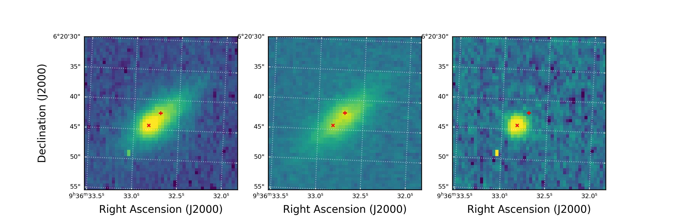
Figure 1: Left: An $r$-band image of SN 2018hfm and its host galaxy taken on 14 Dec. 2018. Middle: A very late-time image taken when SN 2018hfm had faded away. Right: The difference image obtained by subtracting the middle image from the left one. The red cross in the image denotes the location of SN 2018hfm, while the red plus sign marks the centre of the host galaxy.

SN 2018hfm was discovered and first reported on 9 Oct. 2018 at 15:07:12.00 (UT dates are used throughout this paper; MJD = 58400.630) by the ASASSN (All-Sky Automated Survey for Supernovae) team (Stanek, 2018), with J2000 coordinates of $\alpha=09^{\rm h}36^{\rm m}08.736^{\rm s}$ and $\delta=+06^{\circ}15^{\prime}27.08^{\prime\prime}$. As shown in Figure 1, this source is located $\sim 2.8\arcsec$ northeast from the centre of the host galaxy, PGC 1297331. Two days after the discovery, a blue featureless spectrum was obtained by Zheng et al. (2018), and another spectrum taken one day later shows a shallow absorption due to He i $\lambda$5876, with an expansion velocity of $\sim 7500$ km s^-1 (Nascimbeni et al., 2018). However, neither of these two spectra provides a conclusive classification of SN 2018hfm. Later follow-up spectra identify this transient as a Type II SN with some peculiar characteristics, such as high-velocity features and a box-like profile of H$\alpha$ emission. The host galaxy of SN 2018hfm has redshift $z=0.008$ according to NED (Nascimbeni et al., 2018).

2.1 Photometry

2.1.1 ASASSN and Nickel data

Our multiband photometric observations (see Sec.2.1.2) began on 24 Nov. 2018 (MJD = 58446), $\sim 45$ d after discovery. We supplement these data with earlier observations from ASASSN obtained via the Sky Patrol website (Shappee et al., 2014; Kochanek et al., 2017). After providing coordinates and dates to the website, real-time aperture photometry with zeropoints calibrated using the APASS catalog was automatically applied to the unpublished $V$/$g$-band images, and we obtained the measured fluxes.

Note that the standard method of measuring the SN flux is to perform photometry on the residual image after a reference image is subtracted. However, since raw images were unavailable to us, we adopted an alternative way to estimate the flux of SN 2018hfm using the ASASSN data. We first estimated contamination from the host galaxy by performing real-time aperture photometry on images taken within 400 d before explosion and then calculated the median ($f_{\rm bkg}$) and standard deviation ($\sigma_{\rm bkg}$) of the obtained flux. Then we focused on the flux observed around the discovery time of SN 2018hfm, selecting points higher than $f_{\rm bkg}+3\sigma_{\rm bkd}$ as being definitely detected signals. After subtracting $f_{\rm bkg}$, we obtained the “pure” SN flux; the results are listed in Table 1.

Table 1: SN 2018hfm $V/g$-band ASASSN photometry

MJD	$V$	MJD	$g$
58392.6	>17.97	58401.5	15.04(03)
58400.6	14.97(04)	58404.5	15.10(03)
58414.6	15.70(08)	58426.5	16.44(08)
58417.6	15.87(09)	58437.5	17.26(12)
58430.6	16.42(08)	58439.3	17.03(10)
58432.6	16.59(09)	58443.5	17.43(17)
58436.5	16.42(08)
58442.5	16.70(15)

• Note: numbers in parentheses are uncertainties in units of 0.01 mag.

Images of SN 2018hfm were also obtained by the 1 m Nickel telescope (Nickel, hereafter) at Lick Observatory in the $BVRI$ bands on two nights (MJD = 58419.5 and 58449.5). The data were reduced using an image-reduction pipeline (Ganeshalingam et al., 2010; Stahl et al., 2019). Point-spread-function (PSF) photometry using DAOPHOT (Stetson, 1987) was performed after a template image was subtracted. Several nearby stars were chosen from the Pan-STARRS1 catalog to help calibrate the flux of SN 2018hfm. The results are listed in Table 2. We find that the Nickel data are quite consistent with the ASASSN data, thus enhancing the reliability of the method we used in estimating the flux of SN 2018hfm from the ASASSN Sky Patrol site.

Table 2: SN 2018hfm Photometry from Lick/Nickel

MJD	$B$	$V$	$R$	$I$
58419.488	16.315(025)	15.856(016)	15.486(015)	15.213(018)
58449.486	18.507(145)	17.920(109)	16.753(070)	16.889(115)

• Note: numbers in parentheses are uncertainties in units of 0.001 mag.

2.1.2 TNT data

Multiband photometric data were also collected with the Tsinghua-NAOC 0.8 m Telescope (TNT, hereafter; Huang et al. 2012) at Xinglong Observatory in the Johnson-Cousins $BV$ and SDSS (Sloan Digital Sky Survey) $gri$ bands. All CCD images were preprocessed using standard IRAF routines, including corrections for bias, flat field, and removal of cosmic rays. We performed astrometric calibration on all of our images using the Astrometry.net software (Lang et al., 2012). Then all of the images were reprojected into coordinates of the template using a Python Package reproject. The template was taken on 6 May 2019 (MJD = 58609), 208 d after the discovery, when the SN was dimmer than the TNT detection limit. We subtracted the template from all of the images using hotpants (Becker, 2015) and performed aperture photometry on the residual images to obtain instrumental magnitudes through AstroImageJ (Collins & Kielkopf, 2013). We extracted sources in the template image and performed photometry on them using a bundled program image2xy of the tool Astrometry.net. After cross-matching these sources to the APASS and SDSS catalogs, we obtained the flux-calibrated magnitudes of SN 2018hfm.

All of the photometric data, spanning from 5.4 d to 116.4 d after the explosion, are displayed in Table 3 and Figure 2.

Table 3: SN 2018hfm photometry from the TNT

MJD	$B$	$V$	$g$	$r$	$i$
58446.9	–	–	–	–	16.75(01)
58447.6	18.28(02)	17.42(22)	17.62(01)	16.66(03)	16.85(01)
58449.9	–	17.64(20)	17.84(01)	16.84(01)	–
58452.8	19.30(01)	18.34(01)	18.68(01)	17.41(01)	17.70(01)
58455.8	20.01(01)	19.28(01)	19.49(01)	18.11(01)	18.51(01)
58465.2	–	–	–	18.44(01)	–
58466.8	–	–	–	–	19.39(18)
58467.4	20.43(08)	20.38(24)	20.15(10)	–	–
58468.8	–	–	–	18.52(02)	–
58476.7	–	–	–	18.73(01)	–
58481.2	–	–	20.37(12)	18.87(10)	19.74(23)
58482.8	–	20.76(01)	–	–	–
58484.7	20.70(07)	–	–	–	–
58486.4	–	–	20.71(02)	19.00(06)	–
58487.4	–	20.96(01)	–	–	19.71(42)
58491.1	–	–	20.96(23)	19.13(02)	–
58499.6	–	–	21.04(01)	19.42(09)	20.25(01)
58511.6	–	–	–	–	>20.70(01)
58514.4	21.08(01)	–	–	19.88(15)	–
58515.7	–	–	>21.60	–	–
58525.6	–	–	–	20.20(01)	–
58576.5	–	–	–	>21.12	–

• Note: numbers in parentheses are uncertainties in units of 0.01 mag.

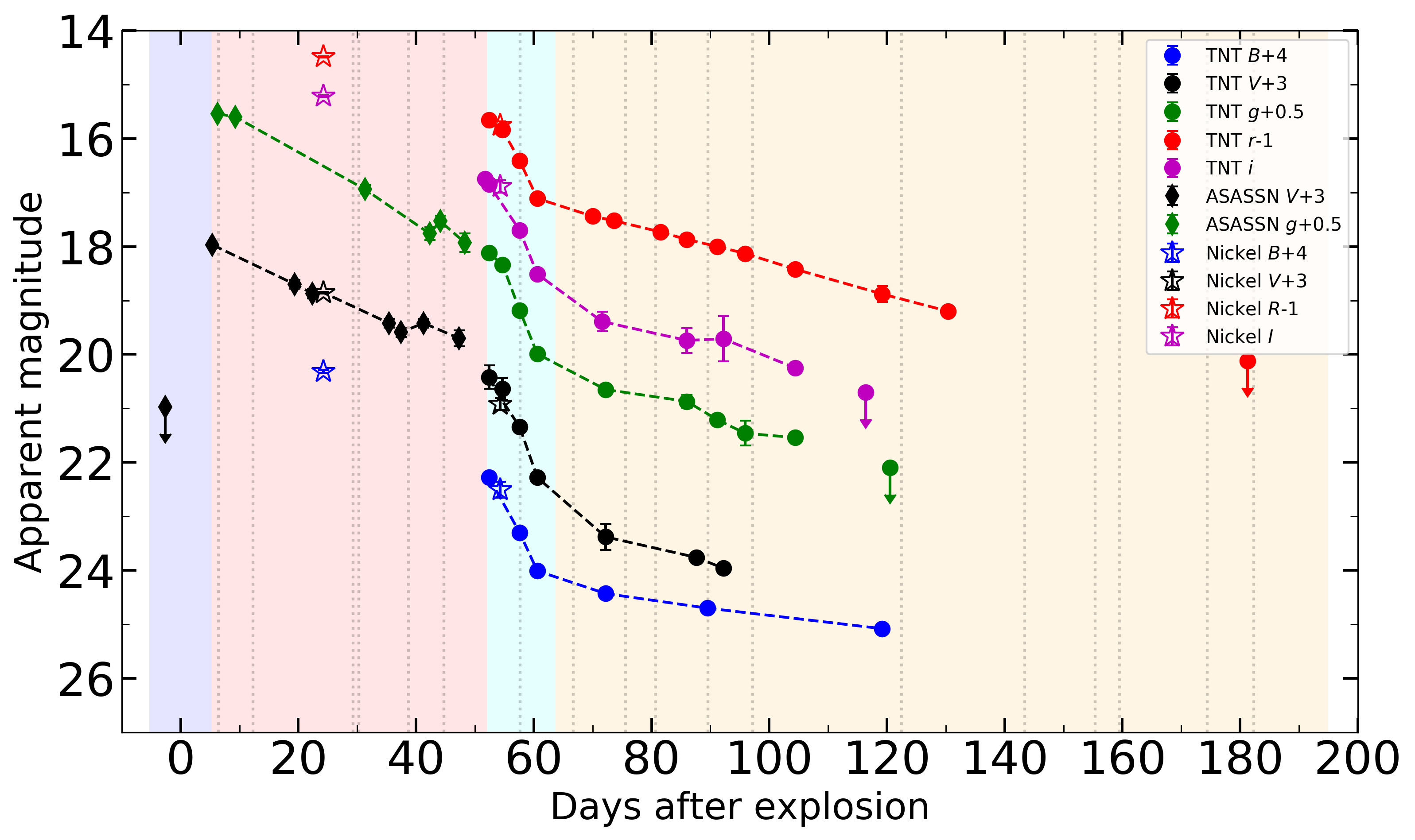
Figure 2: Multiband light curves of SN 2018hfm obtained with the TNT (filled circles), the Lick/Nickel (hollow stars), and from the ASASSN Sky Patrol (diamonds). Data points are shifted vertically, if necessary, for clarity. An upper limit is denoted by a downward arrow. Vertical dashed lines denote spectral epochs and shaded regions show four evolution phases: rising, plateau-like, transitional, and tail (from left to right).

2.2 Spectroscopy

As shown in Figure 3, 19 spectra of SN 2018hfm were obtained: four with the Kast spectrograph (Miller & Stone, 1993) on the 3 m Shane telescope at Lick Observatory (Lick, hereafter), ten with the Beijing Faint Object Spectrograph and Camera (BFOSC) on the 2.16 m telescope at Xinglong Observatory (XLT, hereafter), one with the Dual Imaging Spectrograph (DIS) on the 3.5 m telescope at the Apache Point Observatory (APO, hereafter), two with the Yunnan Faint Object Spectrograph and Camera (YFOSC) on the Li-Jiang 2.4 m telescope of Yunnan Astronomical Observatory (LJT, hereafter; Fan et al. 2015), and two (at late times) with the Low-Resolution Imaging Spectrometer (LRIS) on the Keck-I 10 m telescope (Keck, hereafter; Oke et al. 1995). A Journal of spectroscopic observations is presented in Table 4.

Table 4: Journal of spectroscopic observations of SN 2018hfm

No.	UT Date	MJD	Epoch (day)*	Exp. (s)	Telescope+Inst.	Range (Å)
1	2018-10-10	58401.6	6.4	$2\times 300$	Lick 3m+Kast	3573 - 10642
2	2018-10-16	58407.5	12.3	1500	Lick 3m+Kast	3573 - 10646
3	2018-11-02	58424.5	29.3	1500	Lick 3m+Kast	3587 - 10640
4	2018-11-03	58425.5	30.3	1800	Lick 3m+Kast	3585 - 10639
5	2018-11-11	58433.9	38.7	3300	XLT+BFOSC	3817 - 8627
6	2018-11-17	58439.9	44.7	3000	XLT+BFOSC	3820 - 8627
7	2018-11-30	58452.9	57.7	3000	XLT+BFOSC	3821 - 8627
8	2018-12-09	58461.9	66.7	3300	XLT+BFOSC	3941 - 8621
9	2018-12-18	58470.8	75.6	3300	XLT+BFOSC	3941 - 8617
10	2018-12-23	58475.9	80.7	3300	XLT+BFOSC	3945 - 8622
11	2019-01-01	58484.8	89.6	3600	XLT+BFOSC	3818 - 8621
12	2019-01-09	58492.4	97.2	1800	APO+DIS	5321 - 9081
13	2019-02-03	58517.7	122.5	2098	LJT+YFOSC	3471 - 8696
14	2019-02-24	58538.6	143.4	3600	XLT+BFOSC	4337 - 8634
15	2019-03-08	58550.6	155.4	3600	XLT+BFOSC	4070 - 8752
16	2019-03-12	58554.7	159.5	3600	XLT+BFOSC	3827 - 8751
17	2019-03-27	58569.6	174.4	2400	LJT+YFOSC	3475 - 8694
18	2019-04-04	58577.5	182.3	607.5	Keck I+LRIS	3160 - 10196
19	2019-10-28	58784.6	389.4	900.0	Keck I+LRIS	3112 - 10204

• The epoch is relative to the explosion date, MJD = 58395.2.

The spectra from XLT, LJT, and APO were reduced using standard IRAF routines including bias correction, flat fielding, and removal of cosmic rays. The wavelengths were calibrated through a dispersion solution from suitable lamp spectra. Flux calibration was obtained using standard stars observed at similar airmass on the same night. The spectra were further corrected for continuum atmospheric extinction and removal of telluric lines as far as possible. Keck spectra were reduced with the standard procedures described by Silverman et al. (2012).

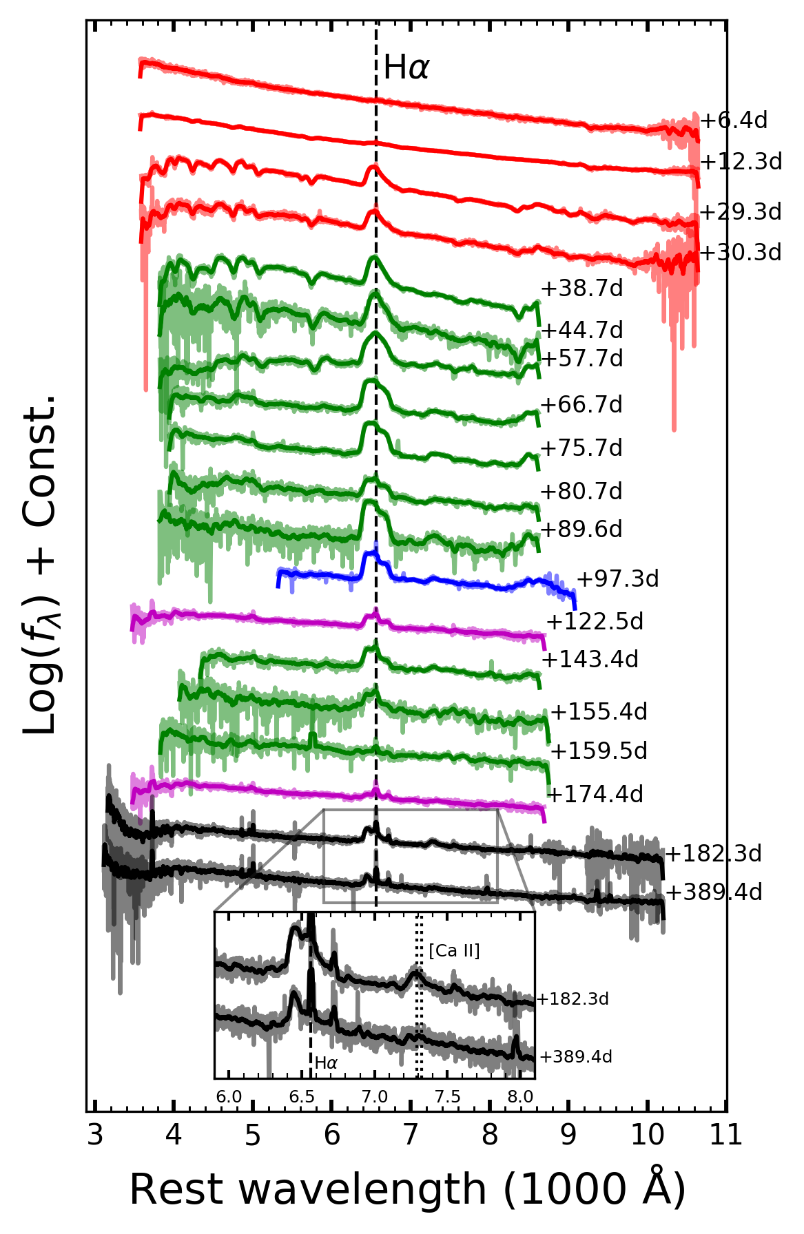
Figure 3: Optical spectroscopic evolution of SN 2018hfm. All of the spectra have been corrected for the redshift and extinction. They are smoothed (bold lines) and shifted vertically for better clarity. The phase after explosion (MJD = 58395.2) is marked on the right side of each spectrum. The last two spectra are partially zoomed-in for better display of the $\rm H\alpha$ and [Ca ii] emission lines. Spectra from different instruments are shown in different colours, with red representing spectra from Lick, green from XLT, blue from APO, magenta from LJT, and black from Keck.

3 Estimation of extinction and distance

To estimate extinction both from the host galaxy and the Milky Way, we measured the equivalent width (EW) of Na i d from the Lick spectrum taken on 2018 Oct. 16. This high-quality spectrum is characterised by a blue continuum with shallow Balmer absorption lines. As shown in Figure 4, we can identify two Na i d systems in the spectrum; that from the Milky Way is at the rest wavelength of Na i d, and the redshifted one is caused by the host galaxy. Measurement of these two absorption lines gives us the EW of Na i d from the Milky Way as EW${}_{\rm MW}=0.28$ Å and that from the host as EW${}_{\rm host}=0.88$Å. The results derived from four empirical formulae transforming the EW of Na i d to $E(B-V)$ are listed in Table 5. The median values and standard deviations are $E(B-V)_{\rm MW}=0.06\pm 0.03$ mag and $E(B-V)_{\rm host}=0.26\pm 0.10$ mag.

Figure 4: Identification of Na i d absorption lines from the host galaxy and the Milky Way. The spectrum shown was taken on 2018 Oct. 16 (12.3 d after explosion) with the 3 m Shane telescope at Lick Observatory. The left vertical dashed lines denote Na i d absorption from the Milky Way and the right ones denote the trough due to the host galaxy. The red straight line is the presumed continuum. Bold dashed troughs under the spectrum are normalised absorption lines used to calculate equivalent width.

Meanwhile, we retrieve the Milky Way dust map from Schlegel et al. (1998) and find the line-of-sight reddening toward SN 2018hfm to be $E(B-V)=0.05$ mag, consistent with the above result estimated from Na i d absorption lines. To double check the reddening due to the host galaxy, we adopt the Balmer-decrement method (Osterbrock, 1989). The principle of this method is that quantum physics determines the intrinsic flux ratio of $\rm H\alpha$ to $\rm H\beta$, and any deviation can be attributed to dust extinction. From the SDSS spectrum of the host galaxy (Adelman-McCarthy et al., 2008), as shown in Figure 5, we measure a Balmer decrement of 4.56. As the SDSS spectrum was taken toward the host-galaxy centre and SN 2018hfm is quite near the centre, we do not expect a large deviation from the true value. According to Equation 4 of Domínguez et al. (2013), we estimate the host-galaxy reddening to be $E(B-V)_{\rm host}=0.40$ mag. This result is also consistnent with that estimated from the Na i d absorption.

Finally, we choose $E(B-V)$ of the Milky Way and the host galaxy to be 0.05 mag and 0.26 mag, respectively, resulting in a total reddening of $E(B-V)=0.31$ mag. Assuming a total-to-selective extinction ratio $R_{V}=3.1$ (Cardelli et al., 1989), we obtain $A_{V}=R_{V}\times E(B-V)=0.96$ mag and $A_{B}=1.27$ mag, as well as $A_{g}=1.02$ mag, $A_{r}=0.72$ mag, and $A_{i}=0.53$ mag (Yuan et al., 2013, Table 2).

HyperLeda, a galaxy database, provides distance information for the host galaxy, PGC 1297331. Three distance moduli exist in the database: one is “mod0” calculated from their distance catalogue independent of redshift; another is “modz” computed from the redshift with H${}_{0}=70$ km s^-1 Mpc^-1, $\Omega_{M}=0.27$, and $\Omega_{\Lambda}=0.73$; and the last is “modbest,” a weighted average of “mod0” and “modz.” We adopt “modbest” as our final distance modulus, giving a value of $32.70\pm 0.64$ mag and corresponding to $D_{L}=34.67\pm 9.64$ Mpc.

Table 5: Reddening derived from different methods

Relation	$E(B-V)_{\rm MW}$*	$E(B-V)_{\rm host}$**	reference
0.25EW	0.07	0.22	Barbon et al. (1990)
0.16EW-0.01	0.03	0.13	Turatto et al. (2003)
0.51EW-0.04	0.10	0.41	Turatto et al. (2003)
0.43EW-0.08***	0.04	0.30	Poznanski et al. (2012)
median	0.06	0.26
standard deviation	0.03	0.10

• EW of Na i d from the Milky Way is 0.28 Å.

• EW of Na i d from host is 0.88 Å.

• This formula requires EW $<1$ Å.

4 Host Galaxy: PGC 1297331

The host of SN 2018hfm, PGC 1297331, is classified as a transition-type dwarf (TTD) galaxy (Koleva et al. 2013; SDSS J0936 in their sample), which presents characteristics between those of irregular and elliptical galaxies. SDSS provides a spectrum taken toward the centre of PGC 1297331 (Adelman-McCarthy et al., 2008), as shown in Figure 5.

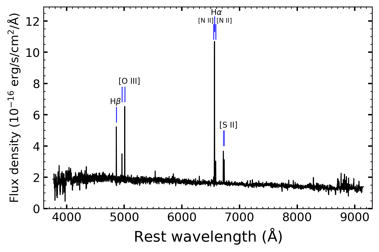
Figure 5: SDSS spectrum of the host galaxy of SN 2018hfm, PGC 1297331. Some strong lines are denoted.

4.1 Metallicity

To determine the metallicity of the host environment, we measured the flux ratios of some strong emission lines in the SDSS spectrum of PGC 1297331, including $N2=\log_{10}([\text{N\,{ii}}]\lambda 6584/\text{H}\alpha)$, $O3=\log_{10}([\text{O\,{iii}}]\lambda 5007/\text{H}\beta)$, and $O3N2=\log_{10}(([\text{O\,{iii}}]\lambda 5007/\text{H}\beta)/([\text{N\,{ii}}]\lambda 6584/\text{H}\alpha))$. The results are $N2=-0.783$, $O3=0.286$, and $O3N2=1.069$. The values of $N2$ and $O3$ satisfy $O3<0.61/((N2-0.05)+1.3)$, suggesting no contamination from an active galactic nucleus (Kauffmann et al., 2003). We then calculated the gas-phase oxygen abundance as 8.388 dex (0.5 Z_⊙) from $O3N2$ based on the relation derived by Pettini & Pagel (2004). This value indicates that SN 2018hfm has a relatively metal-poor host environment compared to other SNe II (Dessart et al., 2014; Anderson et al., 2016).

4.2 Star-formation rate

We retrieved a background-subtracted and flux-normalised far-ultraviolet (FUV) intensity map of PGC 1297331 from the GALEX Catalog. We performed photometry on the galaxy with an elliptical aperture using the photutils Python package (Bradley et al., 2017), where the aperture parameters are adopted from HyperLeda. The measured flux was converted into AB magnitude (Oke & Gunn, 1983) using the zero point defined by Equation 3 of Morrissey et al. (2007). After applying Galactic and intrinsic extinction using Equation 4 of Karachentsev & Kaisina (2013), we obtained the extinction-corrected FUV magnitude of PGC 1297331, $m_{\rm FUV}^{\rm c}=18.57$ mag. We then transformed the FUV magnitude into the star-formation rate (SFR) using Equation 3 of Karachentsev & Kaisina (2013), namely $\log(\rm SFR[M_{\odot}\,yr^{-1}])=2.78-0.4m_{\rm FUV}^{\rm c}+2\log(D[\rm Mpc])$. Given $D=34.67$ Mpc, the SFR can be calculated as $0.0270\,\rm M_{\odot}\cdot\,yr^{-1}$. Chang et al. (2015) report $\sim 0.021\,\rm M_{\odot}\,yr^{-1}$ as a median SFR estimate for the whole galaxy, thus verifying our result.

We adopt $0.0270\,\rm M_{\odot}\,yr^{-1}$ as the SFR of PGC 1297331. This SFR corresponds to a low CCSN rate of $\sim 1$ SN per 5000 yr, which is 1–2 orders of magnitude below that of the hosts of the CCSNe discussed by Botticella et al. (2012).

5 Photometric evolution

The overall evolution of the SN 2018hfm light curves is shown in Figure 2. These multiband light curves reveal four evolutionary stages: a rising phase, a plateau-like phase, a rapid-dropping transition, and a tail phase. For the plateau-like phase, SN 2018hfm presents special features — a fast decline rate and short duration.

5.1 Explosion date and rise time

Gutiérrez et al. (2017) describe two methods to determine the explosion epoch. One is to set it as the midpoint between the last nondetection date (MJD_nondet) and the discovery date (MJD_disc), along with the representative uncertainty determined by $(\rm MJD_{disc}-\rm MJD_{nondet})/2$. Another is to perform a comparison between the observed spectra at early times and SNID templates (Blondin & Tonry, 2011) to find a best-fit spectral phase. Applying these two methods to their SN II sample, Gutiérrez et al. (2017) find a mean offset of 0.5 d between them. These two methods have also been used by Anderson et al. (2014) to determine explosion epoch when they analysed their SN II sample; However, they find an offset of 1.5 d between the two methods.

The earliest detected photometric point of SN 2018hfm, obtained from ASASSN Sky Patrol, was taken on MJD = 58400.6 with a value of 14.97 mag in the $V$ band. Given that the magnitude is brighter than any later ones in $V$, we consider this point to be the peak of the $V$ light curve. Eight days before this peak (i.e., MJD = 58392.6), an upper limit in $V$ ($>17.97$ mag) was also provided by ASASSN. After correcting for extinction, we converted the peak magnitude and the upper limit to an effective flux density $f$ of 9.0 and 0.57 (in units of $10^{-15}$ erg s^-1 cm^-2 Å^-1), respectively. We then fit a simple formula, $f(t)\propto t^{2}$ (Arnett, 1982), to the above two data points, and let $f(t)=0$ to obtain the earliest possible explosion epoch, MJD = 58389.9. Assuming this date as the MJD_nondet and the time of peak brightness as the MJD_disc, we determine the explosion epoch as MJD $=58395.2\pm 5.3$, according to the first method.

Table 6: Best-fit spectral templates from SNID

SN name	days from explosion	SN name	days from explosion
SN 2006bp	+12.59	SN 1999em	+8.3
SN 2006iw	+11.0	SN 2008in	+4.0
SN 2009bz	+9.0	SN 1999gi	+7.7
SN 2004fc	+9.0	SN 2004et	+13.18
mean	+9.4*	$\sigma$	2.8

• The compared spectrum of SN 2018hfm was taken on MJD = 58407.5. Therefore, a phase estimate of $+9.4\pm 2.8$ d after explosion corresponds to an explosion epoch of MJD $=58398.1\pm 2.8$.

In the second method, we compare our spectrum taken on MJD = 58407.5 with SNID templates. We focus on the wavelength between 3500 Å and 6000 Å, because spectral lines in this region evolved with time consistently, while the $\rm H\alpha$ profile at redder wavelengths varies between SNe so it does not aid in spectral matching (Gutiérrez et al., 2017). The best-fit template spectra are listed in Table 6. The mean value and standard deviation of the phase from these matched spectra thus gives us an alternative estimate of the explosion epoch, MJD $=58398.1\pm 2.8$. This value is offset by 2.9 d from the first result, which is larger than the mean offset proposed by Gutiérrez et al. (2017) (0.5 d) and Anderson et al. (2014) (1.5 d). We attribute this large offset to a relatively low metallicity (0.5 Z_⊙) of SN 2018hfm, as SNe with lower metallicity tend to exhibit metal lines of similar intensity at a phase later than their counterparts with higher metallicity (Dessart et al., 2014).
We adopt the more conservative (with the larger uncertainty) value, MJD $=58395.2\pm 5.3$, as the explosion epoch for SN 2018hfm.

5.2 Light-curve parameters

Statistical studies of SNe II are usually first based on parameters measured from $V$-band light curves (e.g., Anderson et al. 2014; Valenti et al. 2016). Thus, in this subsection, we perform a detailed analysis of the $V$ light curve of SN 2018hfm.

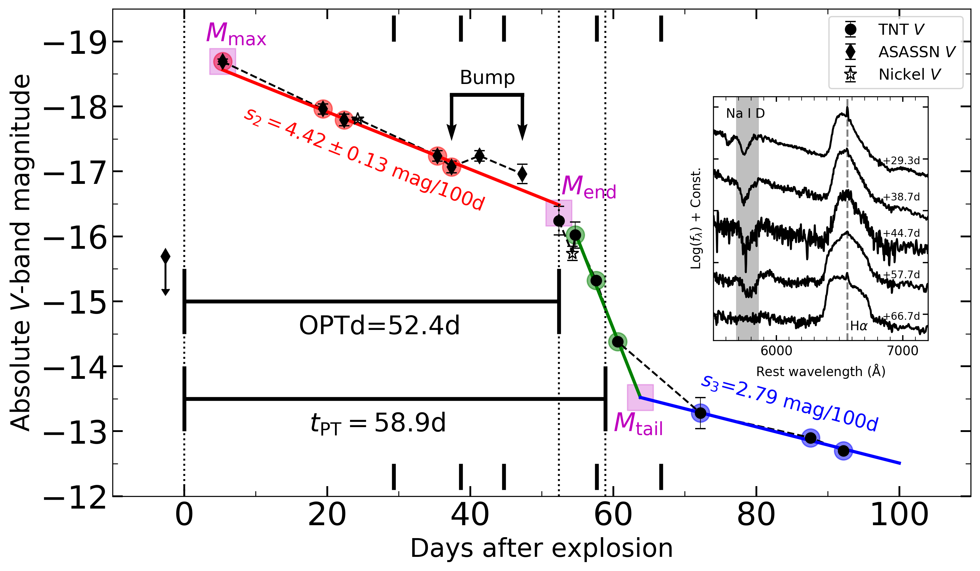
Figure 6: Measuring parameters from extinction-corrected absolute $V$-band light curve. Data are represented with black diamonds (from ASASSN), hollow stars (from Nickel), and circles (from TNT). Three straight lines (red/green/blue) are fitted to the data points circled with the same colour, to determine the decline rate of the plateau ($\rm s_{2}$) and of the tail ($\rm s_{3}$). Three magnitudes ($M_{\rm max}$, $M_{\rm end}$, and $M_{\rm tail}$) are denoted by magenta squares. Values of the optically-thick duration (OPTd) and $t_{\rm PT}$ are marked. The small bump at the end of the plateau-like phase is indicated by two linked arrows. Short black bars mark the spectral epochs shown in the inset.

Following the analysis method described by Anderson et al. (2014), we select 5 points in the plateau-like phase, 3 points in the transition phase, and 3 points in the tail phase, fitting each of them with a straight line as shown in Figure 6. Note that the last two points at the plateau phase, which tend to form a small “bump,” are excluded in the fitting. The decline rates measured for the plateau-like phase and the tail phase are dubbed $s_{2}$ and $s_{3}$, respectively, according to the definition given by Anderson et al. (2014). For SN 2018hfm, $s_{2}$ is measured to be $4.42\pm 0.13$ mag (100 d)^-1 and $s_{3}=2.79$ mag (100 d)^-1.

As mentioned in Section 5.1, we regard the first detected point as the peak of the $V$-band light curve, so that the maximum magnitude ($M_{\rm max}$) and the corresponding time ($t_{\rm max}$) can be determined. We assume that the ending of the plateau ($t_{\rm end}$) arrives +52.4 d after explosion, thus the optically-thick duration (OPTd) is determined as shown in Figure 6. To estimate the $V$-band magnitude at the end of the plateau ($M_{\rm end}$), we extrapolate the first straight line (the red one in Figure 6) until $t_{\rm end}$ and get an inferred magnitude. We then average it with the observed magnitude at the same time (i.e., the first data point from TNT), and adopt the mean value as $M_{\rm end}$. For $t_{\rm tail}$ and $M_{\rm tail}$ (i.e., the beginning time and magnitude of the tail phase), we extrapolate the second (green) and the third (blue) lines in Figure 6) to let them intersect each other, and then we take the corresponding values at the intersection point. The middle-plateau time ($t_{\rm mid}$) is calculated as $(t_{\rm max}+t_{\rm end})/2$ and the corresponding magnitude ($M_{\rm mid}$) is inferred from the best-fit straight line. All of the parameters mentioned above are listed in Table 7.

Table 7: Parameters measured from the absolute $V$-band light curve.

$t_{\rm max}$*	$M_{\rm max}$	$t_{\rm end}$	$M_{\rm end}$	$t_{\rm tail}$	$M_{\rm tail}$
+5.4	$-18.69\pm 0.64$	+52.4	-16.36	+63.8	-13.52
$t_{\rm mid}$	$M_{\rm mid}$	$s_{2}$**	$s_{3}$**
+28.9	-17.52	$4.42\pm 0.13$	2.79$\Delta$

• Days relative to explosion epoch (MJD = 58398.1).

• $s_{2}$ and $s_{3}$ are in units of mag (100 d)^-1.

• $s_{3}$ is obtained by fitting data points directly. We do not trust the data uncertainties in the tail phase.

We caution that the determination of some of the above parameters is somewhat arbitrary, so we apply an alternative method to solve this problem. According to Olivares E. et al. (2010) and Valenti et al. (2016), light curves of SNe II during the transition and the tail phase can be described well by the formula

$$y(t)=\left(\frac{-a_{0}}{1+e^{(t-t_{\rm PT})/\omega_{0}}}\right)+(p_{0}\,t+m_{0}),$$ (1)

where the first term is a Fermi-Dirac function describing the shape of the transition and the second term is a straight line describing the evolution of the tail. Here, $a_{0}$ reflects the depth of the transitional drop, $t_{\rm PT}$ reflects the length of the plateau (which is 58.9 d for SN 2018hfm; see also Figure 6), $\omega_{0}$ represents the timescale of the transition phase, $p_{0}$ (in units of mag d^-1) has a meaning similar to that of $s_{3}$ (i.e., decline rate of the tail), and $m_{0}$ is an intercept related to the brightness of the tail phase. We fit all of the $BVgri$-band light curves during the transition and tail phase with the above formula; the results are listed in Table 8.

Table 8: Fitting parameters (Eq. 1) of multiband light curves.

band	$a_{0}$	$t_{\rm PT}$	$\omega_{0}$	$p_{0}$	$m_{0}$
	(mag)	(d)	(d)	(mag d-1)	(mag)
$B$	2.00	57.4	1.74	0.0137	-14.52
$V$	2.52	58.9	2.06	0.0278	-15.30
$g$	1.94	57.6	1.50	0.0308	-15.84
$r$	1.21	57.7	0.95	0.0294	-17.07
$i$	2.16	58.5	2.08	0.0248	-15.65

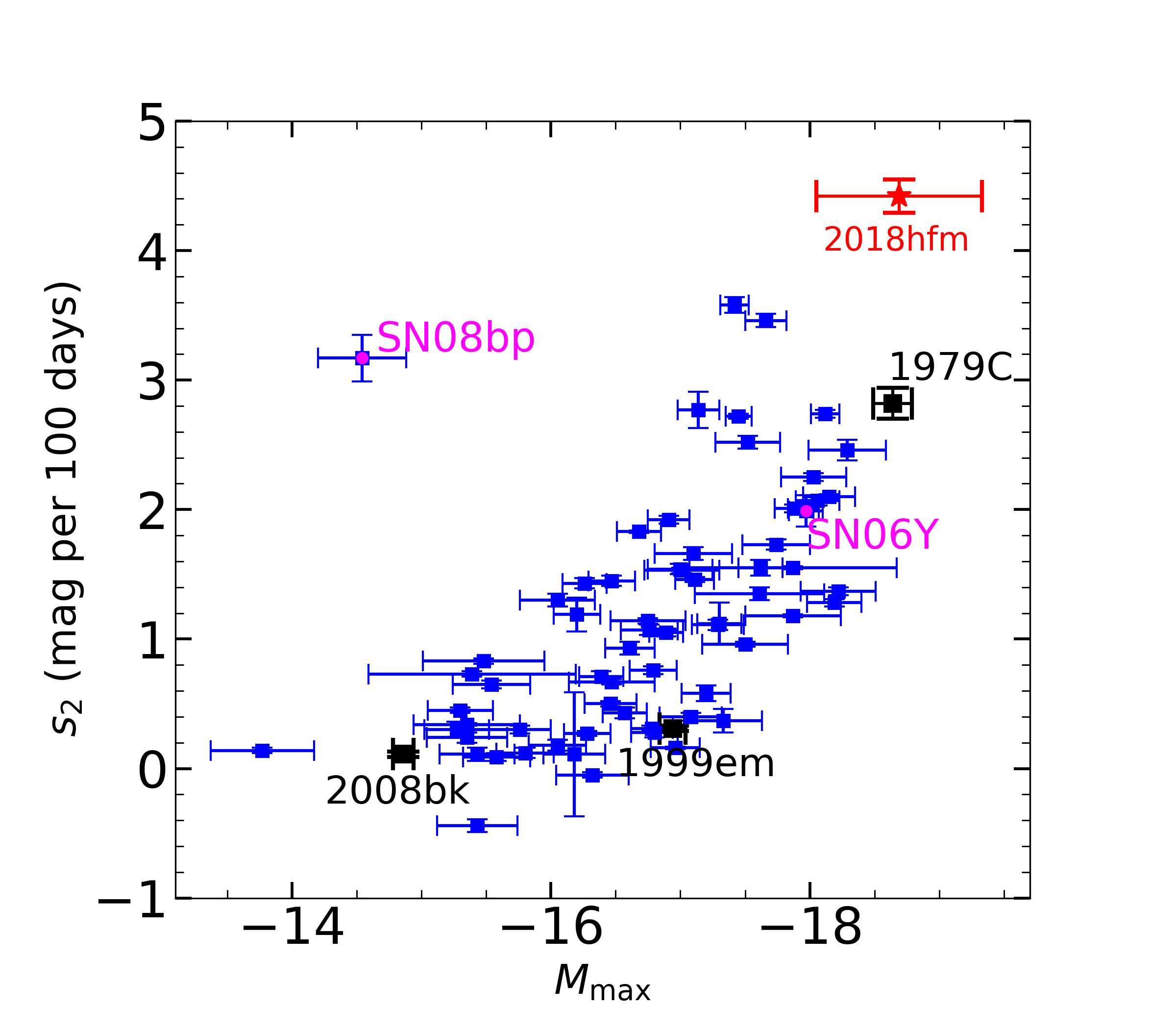
Figure 7: Relationship between absolute $V$-band magnitude at maximum brightness and decline rate of plateau-like phase inherited from Anderson et al. (2014). Their 68 samples are denoted by blue squares with error bars. The subluminous SN 2008bk, prototype SN IIP 1999em, and prototype SN IIL 1979C are denoted by black squares. Fuchsia dots label the outlier SN 2008bp and the peculiar SN 2006Y. SN 2018hfm is denoted by a red star.

Normal SNe IIP usually have a plateau phase lasting for $\sim 100$ d. The estimate of OPTd (52.4 d) and $t_{\rm PT}$ (58.9 d) for SN 2018hfm, however, indicate that it belongs to short-plateau SNe (Hiramatsu et al., 2020). SNe II with a short plateau tend to have large decline rates during the plateau-like phase (see Figure 5(a) of Valenti et al. 2016). This is the case for SN 2018hfm, which indeed has a large value of $s_{2}$ ($4.42\pm 0.13$ mag (100 d)^-1). A more significant and widely accepted relation is between $M_{\rm max}$ and $s_{2}$, where more-luminous SNe II tend to decline faster (Anderson et al., 2014). To show that SN 2018hfm conforms to this relation, we replot Figure 7 of Anderson et al. (2014) by including SN 2018hfm (see Figure 7). The upper-right location of SN 2018hfm reveals its exceptionally high luminosity and rapid decline rate. More cases like SN 2018hfm will extend the data coverage and further examine the relation.

The decline rates during the tail phase of SN 2018hfm, whether in $V$ (reflected by $s_{3}$) or in other bands (reflected by $p_{0}$ values listed in Table 8), are all larger than the expected value of the $\rm{}^{56}Co$-to-$\rm{}^{56}Fe$ decay rate if gamma-ray photons are effectively trapped (i.e., 0.98 mag (100 d)^-1). This indicates that leakage of gamma-ray photons occurs, or that the tail-phase light curves are influenced by other energy source (e.g., CSI).

One may notice that a small “bump” emerges at the end of the plateau (see Figure 6). It is observed not only in $V$ but also in $g$ (see Figure 2). To explore the origin of such a bump, which is not normal in SNe II, we select five spectra obtained around the time of the bump — one before (+29.3 d), two during (+38.7 d, +44.7 d), one after (+57.7 d) but during the transition phase, and one (+66.7 d) in the tail phase. These spectra are shown in the inset of Figure 6.

Among the five spectra, the one at +29.3 d has a blackbody-like continuum and P Cygni profiles of hydrogen and metal lines, similar to other SNe II in their photospheric phase. In the +38.7 d and +44.7 d spectra, the top of the $\rm H\alpha$ emission becomes not so smoothly round. At +57.7 d, when the luminosity decreases but does not yet enter the tail phase, the spectrum exhibits a very broad and bell-shaped profile of $\rm H\alpha$ emission, with metal lines still existing. In the +66.7 d spectrum, metal lines such as Na i d are absent, and the continuum becomes flat and featureless; only $\rm H\alpha$ is present, with a box-like shape and a prominent flux deficiency on the red side.

The photometric and spectroscopic features described above can be explained by the coexistence of two main energy sources. One is the thermal energy deposited in the SN envelope by the explosion shock, which corresponds to the main energy source powering the plateau phase for those normal SNe II without CSI. The other energy source comes from the interaction between the SN ejecta and the CSM. For convenience, we call the former as thermal energy component and the latter as CSI component. Note that when the CSI occurred is a problem worth to be discussed. For SN 2018hfm, the thermal energy component dominates during the plateau phase, so spectra during this phase show similar features to other normal SNe II in the photospheric phase, i.e., P-Cygni profiles. The small bump emerging at the end of the plateau can be explained by that the CSI at this time has occurred, thus extra energy from interaction is superimposed on the thermal energy; however, the CSI energy component is still weak at this time, so we do not see obvious box-like profile of $\rm H\alpha$. In the transition phase, the thermal energy component becomes relatively weak, and the interaction component is increasingly important, we thus see a transitional bell-shaped $\rm H\alpha$ emission line in the +57.7 d spectrum. At the tail phase, when the thermal energy is exhausted and the CSI component becomes dominant, the spectra exhibit box-like $\rm H\alpha$ emission lines with a flat, featureless continuum.

To get an idea about the contribution of CSI, we investigate the fraction of H$\alpha$ flux due to CSI at five epochs ($t=$+29.3d, +38.7d, +44.7d, +57.7d and +66.7d). We first calibrate these five spectra with the corresponding photometric data, and then we estimate the H$\alpha$ flux by integrating the spectra between 6267 Å and 6913 Å . This wavelength range corresponds to the inner and outer layers of CSI emission region (see Appendix A). The H$\alpha$ flux measured at $t=$+66.7d is $\sim 2.15\times 10^{-13}$ erg s^-1 cm^-2, which should be resulted primarily from the CSI. Assuming that the H$\alpha$ flux due to CSI does not change significantly during the period from $t=$+29.3d to $t=$+66.7d, then we can roughly estimate the H$\alpha$-flux fraction due to CSI at other four epochs. The results are 12.6% at $t=$+29.3d, 17.4% at $t=$+38.7d, 19.7% at $t=$+44.7d, and 40.9% at $t=$+57.7d, respectively. One can clearly see the CSI component plays an increasingly important role in shaping the H$\alpha$ line.

5.3 Comparison with other SNe

In Section 5.2 we measured the light-curve parameters and compared them with those of statistical samples of Anderson et al. (2014) and Valenti et al. (2016). The comparison has revealed some photometric uniqueness of SN 2018hfm, such as a high luminosity at maximum brightness, a short plateau duration, and a large decline rate of the plateau-like phase. To further examine the peculiarities of this SN II, in Figure 8 we compare the $V$-band light curve of SN 2018hfm with that of some other SNe II.

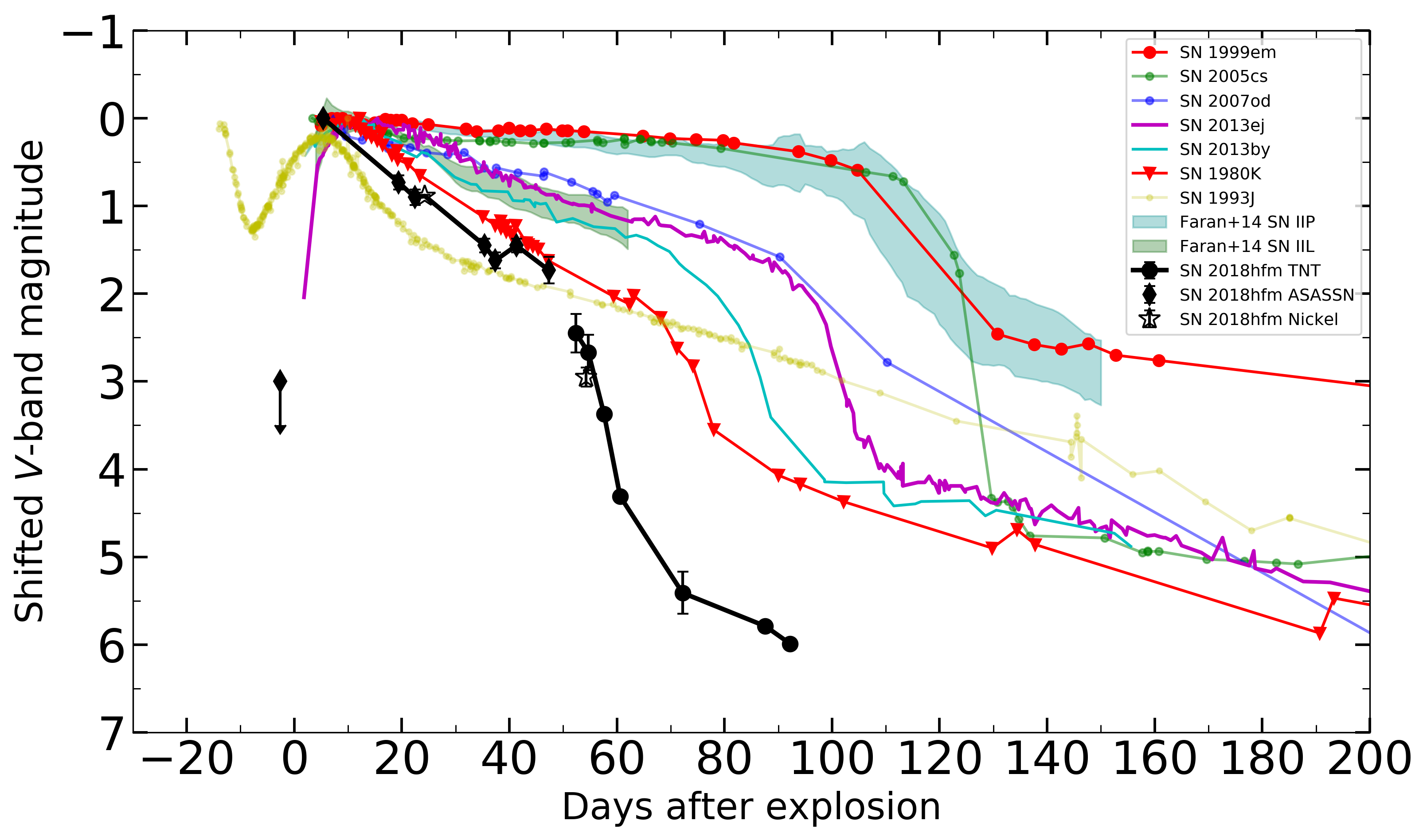
Figure 8: Extinction-corrected absolute $V$-band light curve of SN 2018hfm along with that of other SNe, including prototype SN IIP 1999em (Elmhamdi et al., 2003), prototype SN IIL 1980K (Barbon et al., 1982; Buta, 1982; Marano et al., 1980), prototype SN IIb 1993J (Richmond et al., 1994, 1996), SN 2005cs (Pastorello et al., 2009), SN 2007od (Inserra et al., 2011), SN 2013ej (Huang et al., 2015), SN 2013by (Valenti et al., 2015), and template light curves of SNe II from Faran et al. (2014b). All of the light curves have been shifted vertically to their $V$-band maximum. SN 1993J is also shifted horizontally so that its maximum epoch is aligned with that of SN 2018hfm. The light curves of some SNe are taken from https://sne.space (Guillochon et al., 2017).

As shown in Figure 8, SN 1999em, as a prototype of SNe IIP, shows a long plateau ($\sim 100$ d) with a very slow decline during the plateau phase. SN 2005cs, similar to SN 1999em, also has a typical long plateau. However, SN 2013ej and SN 2013by show a faster decline rate during the plateau-like phase, being in the range of the SN IIL template light curves. These two SNe were observed sufficiently well to catch the final rapid drop at the end of the plateau. SN 2007od tends to have an intermediate plateau drop between that of SNe IIP and SNe IIL. As a prototype of SNe IIL, SN 1980K exhibits a plateau decline rate even larger than that of most SNe IIL examined by Faran et al. (2014b). SN 1993J is a prototype of SNe IIb, which has the most rapid decline rate after its main peak in comparison with other SNe II shown in Figure 6. Regarding the post-peak evolution, one can see that SN 2018hfm lies between SN 1980K and SN 1993J.

As discussed above, light curves of all the SNe II (except SN 1993J) are found to show a four-stage evolutionary sequence. This result is consistent with the fact that progressively more evidence suggests that historically-classified SNe IIP and SNe IIL actually belong to a continuous distribution. Their observational differences are related to the mass of the remaining hydrogen envelope and hence to the mass-loss history of the progenitor stars (Anderson et al., 2014; Valenti et al., 2016; Gutiérrez et al., 2017). Luminous SNe II with short plateaus and large decline rate are likely linked to progenitors having a low-mass envelope, while those with a long plateau, slow decline, and low luminosity are related to progenitors having a high-mass envelope. On the other hand, SNe IIb are believed to retain a very low-mass hydrogen envelope before core collapse (Kilpatrick et al., 2017, and references therein), which may explain the fact that in Figure 8 the light curve of SN 1993J declines fastest after its main peak. The light curve of SN 2018hfm shows a large post-peak decline, which indicates that its progenitor tends to hold a low-mass hydrogen envelope before exploding.

5.4 Bolometic light curve and explosion parameters

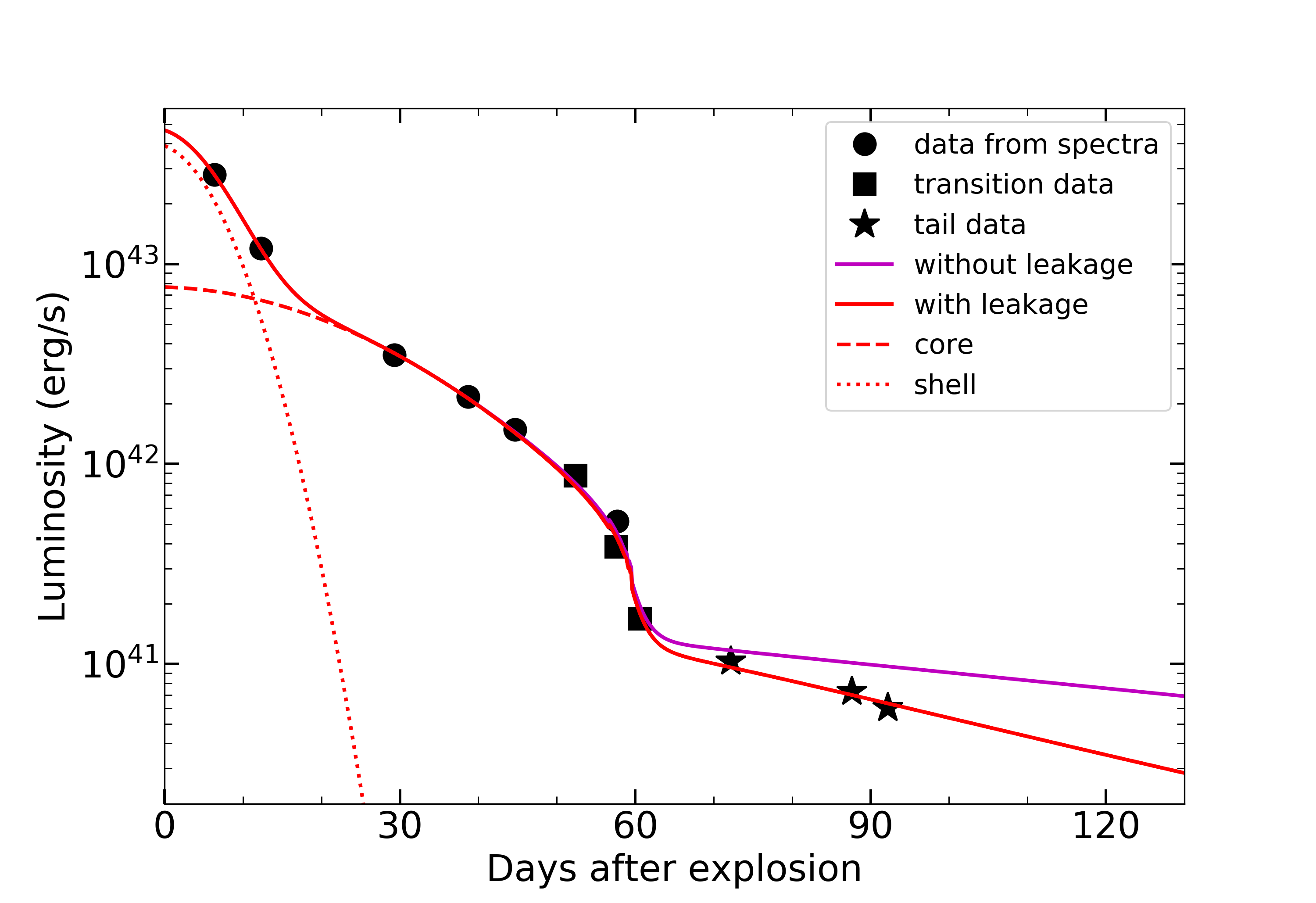
Figure 9: Bolometric light curve of SN 2018hfm (black markers) with LC2 models from Nagy & Vinkó (2016) (red and magenta lines). Parameters related to these lines are listed in Table 9.

In this subsection, we construct the bolometric light curve of SN 2018hfm (see Figure 9) and discuss its properties. During the plateau-like phase we only have $V/g$-band data, but we have collected relatively good-quality spectra (i.e., +6.4 d, +12.3 d, +29.3 d, +38.7 d, and +44.7 d). We calibrate these spectra by the $V$-band magnitude inferred from the best-fit straight line (the red line shown in Figure 6). Note that the straight line does not describe the small bump seen in the ASASSN $V$ and $g$ bands, hence one would not expect a bump feature in the bolometric light curve.

After flux calibration, we perform a blackbody fit to the spectra and integrate it from 1216 Å to infinity; flux at wavelengths shorter than 1216 Å is omitted owing to absorption by the Lyman series (Zhang et al., 2020). We do the same thing for the +57.5 d spectrum, taken during the transition phase, but integrate it from 3600 Å to infinity because blanketing effects of metal lines play a significant role when the temperature decreases. Spectra taken during the tail phase are discarded because the SN was very faint and the continuum could be contaminated by the host galaxy. Multiband ($BVgi$) photometric data taken with the TNT during the transition phase were transformed to spectral energy distributions (SEDs) and then fitted with a blackbody. Similarly, the integration covers the wavelength range from 3600Å to infinity. Note that the $r$-band data are excluded because they are severely influenced by the $\rm H\alpha$ emission produced by CSI. During the tail phase, the bolometric luminosity is reconstructed using the $V$-band data through the following equation (Bersten & Hamuy, 2009; Zhang et al., 2020):

$$\log_{10}L=-0.4[BC+V-A_{V}+11.64]+\log_{10}(4\pi D^{2}),$$ (2)

where $L$ is the luminosity in units of erg s^-1, $D$ is the distance to the SN in units of cm, and $BC$ is the bolometric correction ($-0.7$ mag).

We also present in Figure 9 the bolometric light curves generated by the semi-analytical two-component model (LC2) of Nagy & Vinkó (2016). This model, assuming that the emission can be produced by an inner-core part and an outside-shell part, can be used to investigate explosion parameters of SNe IIP/IIL or SNe IIb. The LC2 parameters are listed in Table 9. It is not surprising that the model with gamma-ray leakage (i.e., $A_{g}\approx 9000$ d²) reproduces the tail if we recall that the values of $s_{3}$ and $p_{0}$ (see Tables 7 and 8) are all larger than 0.98 mag (100 d)^-1.

Table 9: LC2 model parameters of SN 2018hfm.

Parameters*	$R_{0}$ ($10^{13}$cm)	$M_{\rm ej}$ (M⊙)	$M_{\rm Ni}$ (M⊙)	$T_{\rm rec}$ (K)	$E_{\rm kin}$ ($10^{51}$ erg)	$E_{\rm th}$ ($10^{51}$ erg)	$\alpha$	$\kappa$ (cm2 g-1)	$A_{\rm g}$ (d2)
core	10	1.17	0.015	6000	0.22	0.20	1.6	0.28	9000/$+\infty$**
shell	20	0.11	0	0	0.1	0.1	0.0	0.34	$+\infty$

• $R_{0}$ is the initial radius of the ejecta, $M_{\rm ej}$ is the ejected mass, $M_{\rm Ni}$ is the initial nickel mass, $T_{\rm rec}$ is the recombination temperature, $E_{\rm kin}$ is the initial kinetic energy, $E_{\rm th}$ is the initial thermal energy, $\alpha$ is the density profile exponent, $\kappa$ is the opacity, and $A_{\rm g}$ is the gamma-ray leakage exponent.

• $A_{\rm g}=+\infty$ is for the magenta line in Figure 9, representing gamma-ray photons that are fully trapped, while $A_{\rm g}=9000$ is for the red line in Figure 9, representing leakage of the gamma rays.

Among the LC2 parameters, the most important ones are $R_{0}$, $M_{\rm ej}$, and $E_{\rm tot}=E_{\rm kin}+E_{\rm th}$, which control the morphology of the plateau-phase light curve, and $M_{\rm Ni}$, which determines the tail phase. To examine these parameters we also estimate the explosion parameters ($E_{\rm exp}$, $M_{\rm ej}$, $R_{\rm pSN}$) using the following simple approximation formula (Litvinova & Nadezhin, 1985; Zhang et al., 2006):

$$\log_{10}\left(\begin{bmatrix}E_{\rm exp}\\ M_{\rm ej}\\ R_{\rm pSN}\\ \end{bmatrix}\right)=\begin{bmatrix}0.135&2.34&3.13\\ 0.234&2.91&1.96\\ -0.572&-1.07&-2.74\\ \end{bmatrix}\cdot\begin{bmatrix}M_{V}\\ \log_{10}(\Delta t)\\ \log_{10}(v_{\rm ph})\\ \end{bmatrix}-\begin{bmatrix}4.205\\ 1.829\\ 3.350\\ \end{bmatrix},$$ (3)

where $M_{V}$ (in units of mag) is the $V$-band absolute magnitude during the plateau phase, $\Delta t$ (days) is the length of the plateau, and $v_{\rm ph}$ ($10^{3}$ km s^-1) is the photospheric velocity measured +50 d after explosion, while $E_{\rm exp}$ ($10^{51}$ erg), $M_{\rm ej}$ ($\rm M_{\odot}$), and $R_{\rm pSN}$ ($\rm R_{\odot}$) represent the explosion energy, ejecta mass, and initial radius of pre-supernova star, respectively. For SN 2018hfm, owing to a large slope of the plateau, we adopt the magnitude at the midpoint of the plateau (namely $M_{\rm mid}$ in Table 7) as $M_{V}$. Also, the OPTd marked in Figure 6 is regarded as the length of the plateau ($\Delta t$). The value $v_{\rm ph}$ on +50 d is inferred from the velocity evolution of Fe ii $\lambda$5169 measured from spectra (see Figure 13). The parameters calculated through Equation 3 are listed in Table 10, which are consistent with those given by the LC2 model; both indicate a low ejecta mass and low explosion energy for SN 2018hfm compared with SN 1999em or SN 2018zd. (See Table 3 of Zhang et al. 2020; for SN 1999em, they give $M_{\rm ej}=13.50$ M_⊙ and $E_{\rm tot}=1.88\times 10^{51}$ erg in the core part; for SN 2018zd, they give $M_{\rm ej}=9.80$ M_⊙ and $E_{\rm tot}=4.10\times 10^{51}$ erg in the core part.)

Table 10: Explosion parameters calculated from Eq. 3

$M_{V}$ (mag)	$\Delta t$ (d)	$v_{\rm ph}$ ($10^{3}$ km s-1)
-17.52	52.4	3.8
$E_{\rm exp}$ ($10^{51}$ erg)	$M_{\rm ej}$ ($\rm M_{\odot}$)	$R_{\rm pSN}$ ($\rm R_{\odot}$)
0.19	1.63	1750*

• 1750 $\rm R_{\odot}$ = $12.18\times 10^{13}$ cm

5.5 Evolution of colour curves

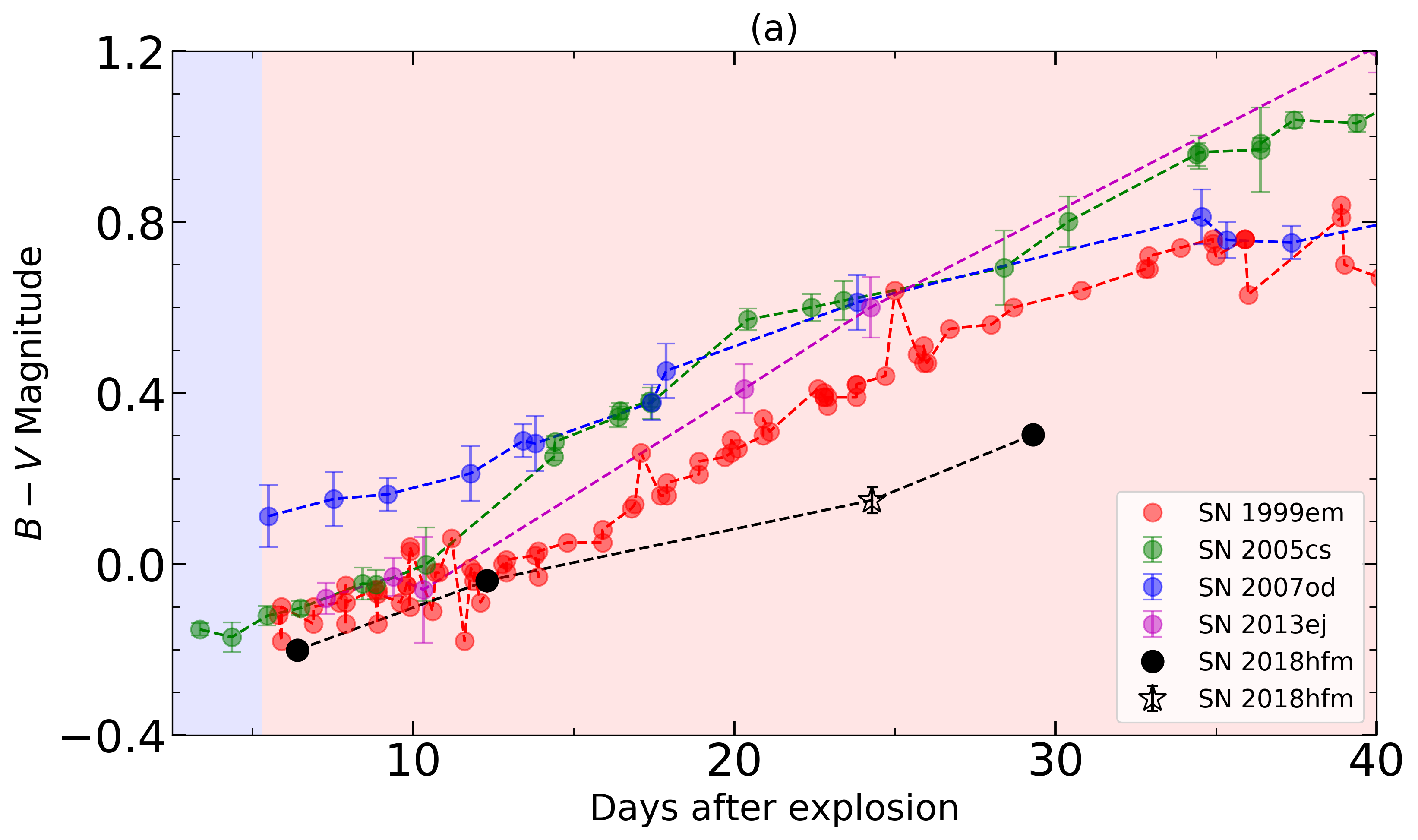
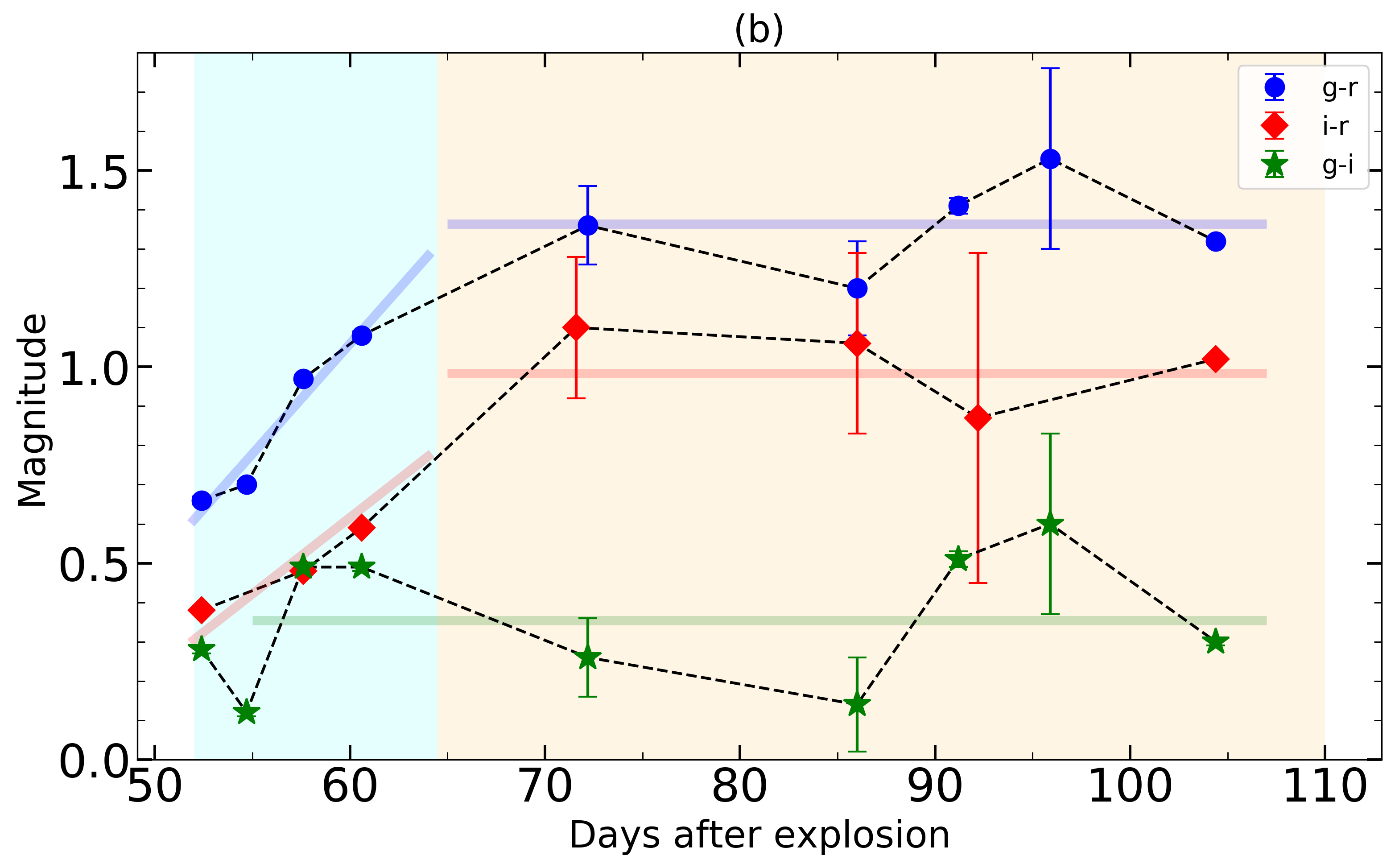
Figure 10: Intrinsic colour curves of SN 2018hfm. Shaded areas represent four evolutionary stages (blue for rise, red for plateau-like phase, cyan for transition, and yellow for tail phase). (a) $B-V$ colour of SN 2018hfm calculated from Nickel photometric data (the hollow star) and from synthetic photometry performed on the early-time spectra (black filled circles), together with $B-V$ colour of SN 1999em (Elmhamdi et al., 2003), SN 2005cs (Pastorello et al., 2009), SN 2007od (Inserra et al., 2011), and SN 2013ej (Huang et al., 2015). (b) $g-r$, $i-r$, and $g-i$ colour curves of SN 2018hfm at the transition and tail phases using photometric data from the TNT. Straight lines show the evolutionary trend of the colour curves.

SN 2018hfm was not well sampled photometrically within one month after the explosion; only the Lick/Nickel telescope took a night of data. However, we collected relatively good-quality spectra during this period. This allows us to perform synthetic photometry with these spectra and obtain the $B-V$ colour. The result is plotted in Figure 10(a), together with those of the comparison samples, including SN 1999em, SN 2005cs, SN 2007od, and SN 2013ej. As can be seen, SN 2018hfm is bluer than the comparison SNe, suggesting a higher temperature in the early phase.

The colour evolution $g-r$, $i-r$, and $g-i$ during the transition and tail phases are shown in Figure 10(b). The value of $g-i$ stays almost unchanged during this time, consistent with the fact that the temperature stays stable and the continuum of the spectra appears very flat. By contrast, values of $g-r$ and $i-r$ both increase (evolving redward) during the transition phase, due to the internal energy deposited by the explosion shock falling and the CSI component gradually dominating the emission. The spectrum from CSI is characterised by strong $\rm H\alpha$ emission, so the $r$ band is brighter than the other bands. During the tail phase, when the CSI component is exposed completely, $g-r$ and $i-r$ stay nearly constant. This means the $\rm H\alpha$ emission and the continuum come from the same energy source (i.e., CSI), which further indicates that the mass of $\rm{}^{56}Ni$ is likely very small and has no significant influence on the tail-phase light curves.

6 Spectroscopic evolution

The complete spectral evolution of SN 2018hfm is displayed in Figure 3, spanning from +6.4 d to +389.4 d after explosion. The first spectrum was taken on +6.4 d, only one day after $V$-band maximum; it is characterised by a very blue and featureless continuum. Applying a blackbody fit to this spectrum indicates a high temperature of $T_{\rm bb}=18,628\pm 94$ K. The second spectrum, taken +12.3 d after explosion, also has a blue continuum but with the appearance of He i $\lambda$5876 absorption, which has a velocity of $\sim 7000$ km s^-1. By $\sim 1$ month after explosion, when the plateau-like phase arrives at its midpoint, metal lines emerge in the spectra. During the transition phase of the light curve, the $\rm H\alpha$ emission shows a strange bell-shaped profile (see discussion in Sec.5.2). When the SN evolves into the tail phase, metal lines become invisible, while broad, boxy $\rm H\alpha$ emission and relatively faint [Ca ii] $\lambda\lambda$7291, 7323 emission dominate the spectra.

6.1 Comparison with other SNe II

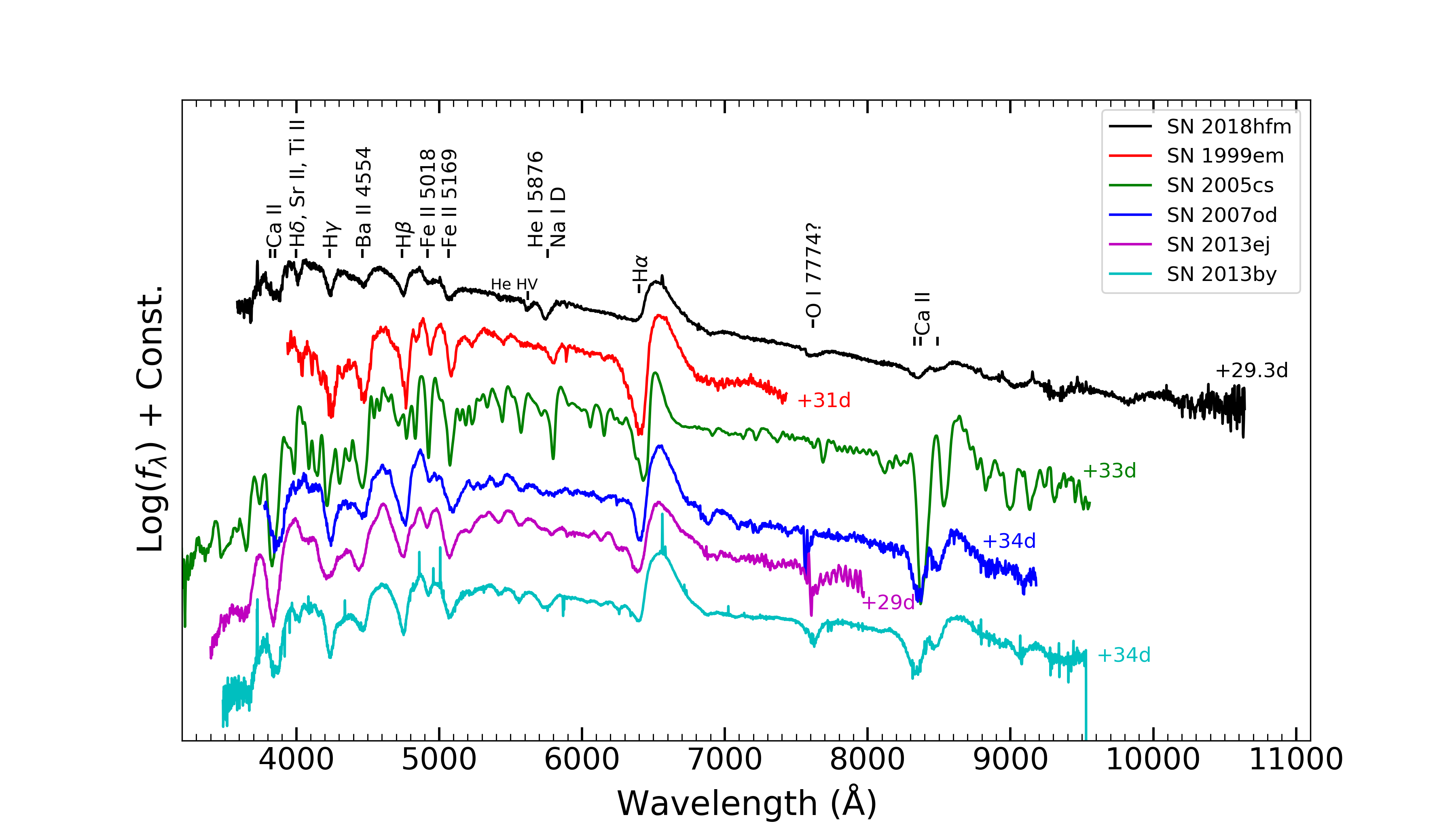
Figure 11: Photospheric spectrum of SN 2018hfm (taken at +29.3 d) compared with that of other SNe II at a similar epoch, including SN 1999em (Elmhamdi et al., 2003), SN 2005cs (Pastorello et al., 2006), SN 2007od (Inserra et al., 2011), SN 2013ej (Huang et al., 2015), and SN 2013by (Valenti et al., 2015). The epoch of each spectrum is denoted on the right side with the same colour. Line identifications are marked by short bars. A high-velocity feature of He i is also marked.

In Figure 11, we compare the +29.3 d spectrum of SN 2018hfm with spectra of SN 1999em, SN 2005cs, SN 2007od, SN 2013ej, and SN 2013by at similar phases. With the comparison, we identify the Balmer series and He i absorption in the spectrum, along with metal lines such as Fe ii, Ca ii, Ba ii, and O i. We notice that a small notch exists on the left side of He i $\lambda$5876 in the +29.3 d spectrum. We checked all of the spectra of SN 2018hfm, and find that this notch also appeared in the +12.6 d spectrum, but it disappeared in the spectral series by +29.3 d and thereafter. This change coincides with a decrement in the temperature, and the notch is likely a high-velocity feature of helium. Moreover, we notice that SN 2018hfm has shallower and fewer metal absorption lines than other SNe II, consistent with the low-metallicity environment (Dessart et al., 2014). The absorption component of the P Cygni $\rm H\alpha$ profile tends to be not well developed for SNe II whose light curve has a fast post-peak decline rate (Schlegel, 1996; Faran et al., 2014b), as indicated by the spectra of SN 2013ej, SN 2013by, and SN 2018hfm.

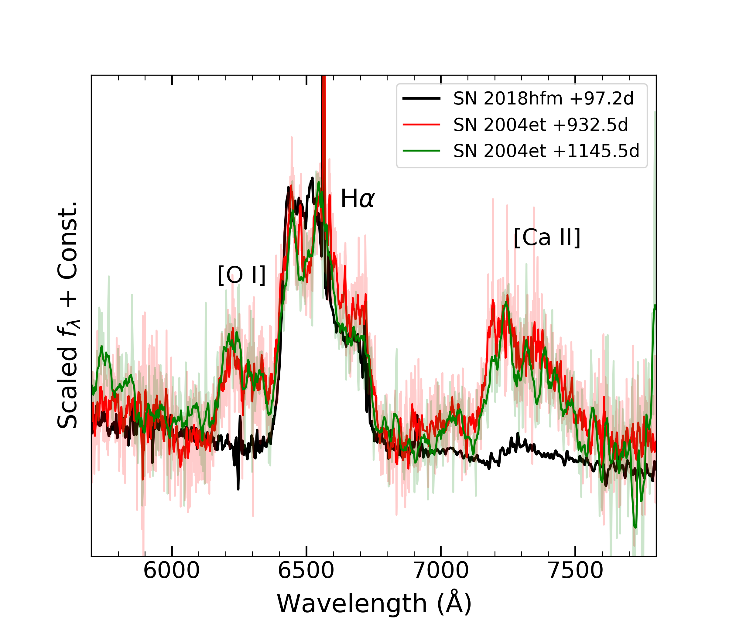
Figure 12: A late-time spectrum of SN 2018hfm compared with two very late-time spectra of SN 2004et (Kotak et al., 2009), showing the similarity in their broad and asymmetric H$\alpha$ profile. The spectra of SN 2004et are smoothed with a boxcar of suitable width.

In Figure 12, we compare a late-time spectrum of SN 2018hfm (+97.2 d) with two very late-time spectra of SN 2004et (+932.5 d and +1145.5 d; Kotak et al. 2009). For the $\rm H\alpha$ emission, SN 2018hfm is quite similar to SN 2004et, both showing asymmetric box-like profiles. According to Jerkstrand (2017), a box-like profile is formed from a shell-like emission region. The maximum velocity at zero intensity (MVZI) of the profile corresponds to the outer boundary of the shell, and the maximum velocity of the flat top is related to the inner boundary. For SN 2014et and SN 2018hfm, this shell-like emission region is believed to have resulted from the collision of the outer ejecta with the CSM. Owing to dust coupled with the emission region, the profile is altered by extinction and scattering to show a red-blue asymmetry (Bevan & Barlow, 2016). Compared with SN 2014et, SN 2018hfm shows no explicit signature of [O i] $\lambda\lambda$6300, 6364, revealing that its progenitor has a very low oxygen abundance and hence a low main-sequence mass (Woosley & Weaver, 1995). Additionally, the [Ca ii] $\lambda\lambda$7291, 7323 emission of SN 2018hfm is still recognisable, meaning a relatively large flux ratio of $R=$ ([Ca ii] $\lambda\lambda$7291, 7323)/([O i] $\lambda\lambda$6300, 6364), which also points to a low-mass progenitor origin for SN 2018hfm (Inserra et al., 2011).

6.2 Evolution of spectroscopic parameters

We measure the temperature and line velocity from the extinction- and redshift-corrected spectra of SN 2018hfm. The temperature is derived by applying blackbody fits to the spectra. For the velocity measurement, we first smooth the spectra when necessary, and then zoom in the absorption trough to judge the minimum by eye. We repeat the measurements by three times and average the results to obtain a final velocity value. The measurements are confined to spectra taken before +60 d since explosion, as tail-phase spectra are dominated by emission features and flat continua which are likely contaminated by the host galaxy.

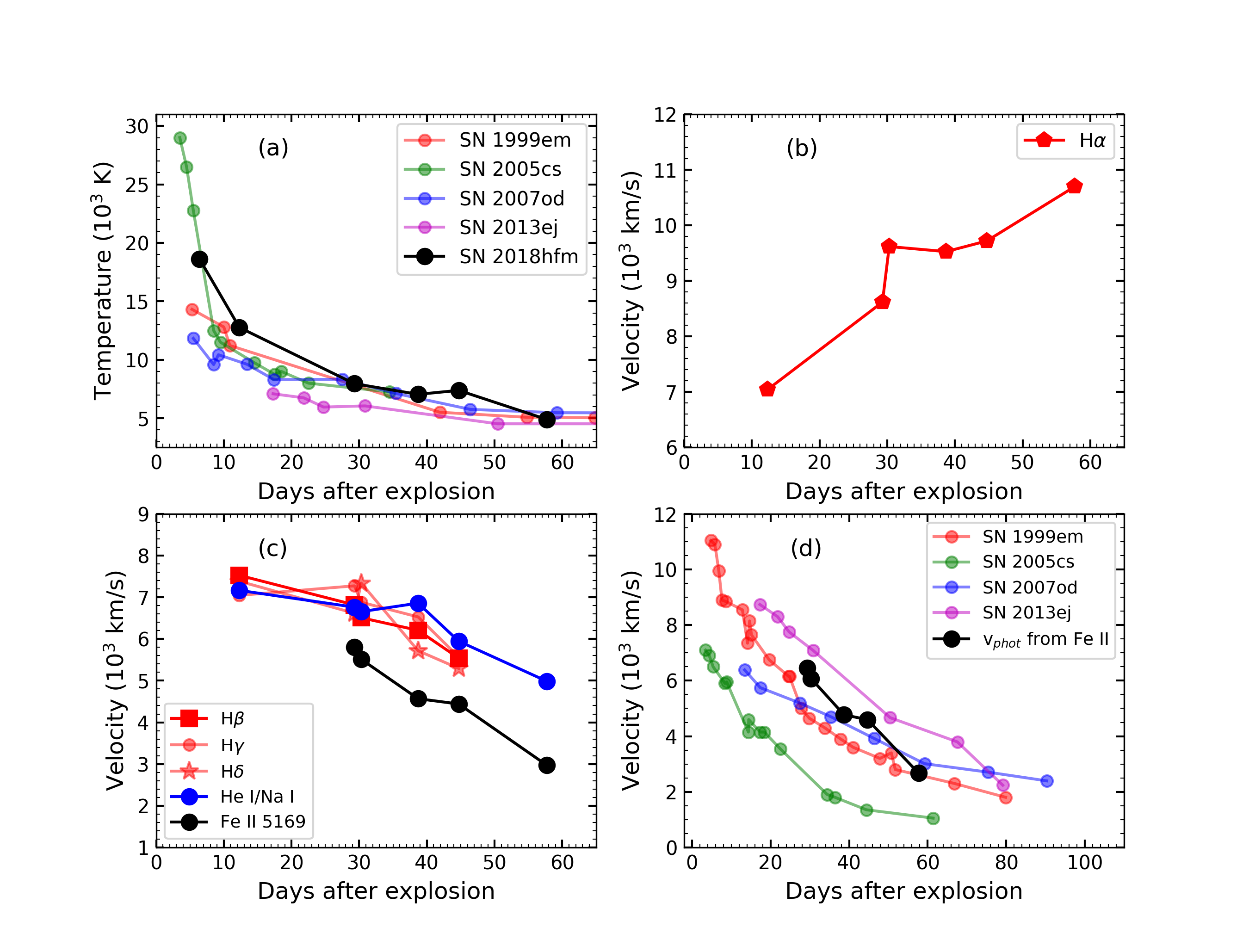
Figure 13: (a) Blackbody temperature evolution of SN 2018hfm compared with that of other SNe II (SN 1999em, Elmhamdi et al. 2003; SN 2005cs, Pastorello et al. 2006; SN 2007od, Inserra et al. 2011; SN 2013ej, Huang et al. 2015). (b) $\rm H\alpha$ velocity of SN 2018hfm inferred from minima of the absorption trough. (c) Line velocity of $\rm H\beta$, $\rm H\gamma$, $\rm H\delta$, He i $\lambda$5876/Na i, and Fe ii $\lambda$5169 measured from spectra of SN 2018hfm. (d) Photoshperic velocity of SN 2018hfm inferred from $v_{\text{Fe\,{ii}}}$ compared with that of other SNe II (Inserra et al., 2011; Takáts & Vinkó, 2012; Huang et al., 2015).

As shown in Figure 13(a), the blackbody temperature of SN 2018hfm is found to be higher than that of SN 1999em and SN 2007od, but similar to SN 2005cs in the early phase. The high temperature of SN 2005cs drops quickly and reaches the same level as SN 1999em and SN 2007od at +10 d, while SN 2018hfm remains hotter than them until one month after explosion. The temperature of SN 2013ej is much lower than that of SN 2018hfm for about two months.

Line velocities are shown in Figure 13(b) and (c). We present the $\rm H\alpha$ velocity in an individual panel to highlight its abnormal evolution. Normally, its velocity should decrease with time like that of other Balmer lines ($\rm H\beta$, $\rm H\gamma$, and $\rm H\delta$ shown in panel (c)), but it accelerates from $\sim 7000$ km s^-1 at +10 d to $\sim 11,000$km s^-1 shortly after the plateau phase. As discussed in the last paragraph of Sec.5.2, the deposited shock energy leads to normal SN evolution, in which line velocities decrease when the photosphere recedes into the deeper layers of the ejecta. However, photons created by CSI come from the outermost ejecta, whose velocity is rather large. These photons tend to fill in the absorption trough of P-Cygni profile and make the through shallower, which will result into a large-velocity measurement. When these photons gradually dominate in the spectrum, it is not unexpected that the H$\alpha$ reveals an abnormal acceleration. The reason $\rm H\beta$, $\rm H\gamma$, and $\rm H\delta$ are not influenced is that the CSI is still in its young phase ($<1$ yr) at this time, and the optical depth is so large that higher-order Balmer-series photons are converted into $\rm H\alpha$ efficiently, leading to a steep Balmer decrement (Chevalier & Fransson, 1994).

As shown in Figure 13(c), He i $\lambda$5876, probably blended with Na i at later phases, evolves similarly to hydrogen, but Fe ii $\lambda$5169 shows a lower velocity. It is consistent with the “onion-ring” structure of elements in progenitors of core-collapse SNe, with light elements lying in outer layers and heavy ones at smaller radii. Evolution of the photospheric velocity can be inferred from Fe ii $\lambda$5169 through an empirical formula (see Eq. 1 of Takáts & Vinkó 2012 with parameters in their Table 2). As shown in Figure 13(d), SN 2018hfm, whose explosion energy is very low, exhibits photospheric velocity comparable to that of other SNe II. This is because the ejecta mass of SN 2018hfm is also much lower than that of the comparison SNe.

6.3 High-velocity features

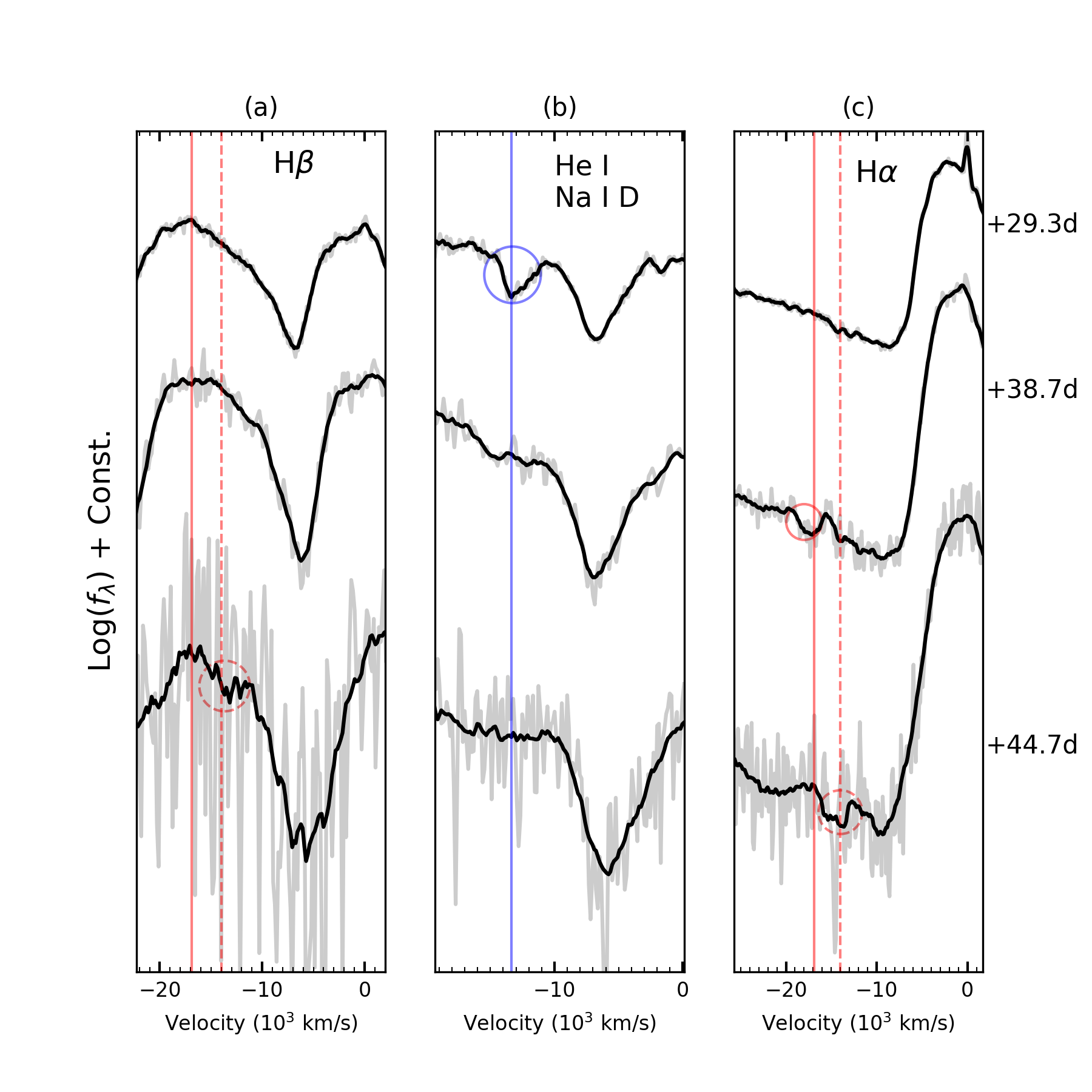
Figure 14: High velocity (HV) features of (a) $\rm H\beta$, (b) He i $\lambda$5876, and (c) $\rm H\alpha$. Solid (dashed) red lines in panels (a) and (c) denote a velocity of $-16,900$ ($-14,000$) km s^-1, with solid (dashed)-edge circles highlighting the HV features. The blue line in panel (b) marks a velocity of $-13,340$ km s^-1, with a blue circle denoting the HV feature of He i. Phases of spectra are labelled at the right side of panel (c). Velocity is relative to the rest wavelength of each line.

In the situation of CSI, X-rays, mainly from the reverse shock, ionise and excite the outer layers of SN ejecta to produce a small depression in the blue wing of the undisturbed absorption component of the P Cygni profile (Chugai et al., 2007; Blinnikov, 2017). This small depression, or high-velocity feature, is observed in many SNe II. For instance, it is reported by Gutiérrez et al. (2017) that 60% of their sample exhibit this feature. We thus inspect spectra of SN 2018hfm to search for possible evidence of such a feature (see Figure 14). As discussed in Section 6.1, the blue notch on the left of He i $\lambda$5876 disappears when the temperature decreases, which favours formation by high-velocity helium. As for hydrogen, if a blue notch in the $\rm H\alpha$ profile is indeed a high-velocity feature, then similar absorptions are expected in the profiles of other hydrogen lines (Faran et al., 2014a; Gutiérrez et al., 2017). Thus, only the small trough with a velocity of $-14,000$ km s^-1 in the +44.7 d spectrum can indeed be a high-velocity feature, while the notch in the +38.7 d spectrum could be a signature of Si ii $\lambda$6355 with a velocity of $-7634$ km s^-1.

6.4 Box-like emission of $\rm H\alpha$ and [Ca ii] at late phase

In this section, we focus on the evolution of $\rm H\alpha$ and [Ca ii] emission lines emerging in the late phases (from +66.7 d to +389.4 d). We apply continuum subtraction and intensity normalisation to the $\rm H\alpha$ emission, and then we define and measure the following parameters from the emission-line profile — the blue/red velocity at zero intensity (BVZI/RVZI), the blue velocity at half-maximum intensity (BVHM), and the velocity of the inner boundary of the shell-like emission region ($V_{\rm in}$) (see detailed description in Appendix A). Results of these parameters are listed in Table 11.

Table 11: Values of parametars defined in Figure 19 and Appendix A.

Phase	BVHM	RVZI	$V_{\rm in}$	BVZI ($V_{\rm out}$)	$V_{\rm in}/V_{\rm out}$	right roof ratio	left roof
(d)	(km s-1)	(km s-1)	km s-1	km s-1			(erg s-1 cm-2 Å-1)
+66.7	-7557.14	16,000	-6500	-13,500	0.48	0.50	1.279e-15
+75.6	-7504.64	15,000	-6400	-11,000	0.58	0.50	7.640e-16
+89.6	-7572.84	12,500	-6766	-10,600	0.64	0.42	3.261e-16
+97.2	-7134.23	12,200	-6245	-10,600	0.59	0.46	6.975e-15
+122.5	-6699.28	10,300	-5848	-9,000	0.65	0.60	3.879e-16
+143.4	-7130.26	10,000	-6100	-10,600	0.58	0.33	3.928e-16
+182.3	-6975.46	8,668	-5480	-8,500	0.64	0.20	1.944e-16
+389.4	-6398.80	8,400	-5686	-7,877	0.72	0.08	6.617e-17

From Figure 15(a) or from the values of BVHM/BVZI listed in Table 11, one can find that the $\rm H\alpha$ box-like profile is very broad, with a velocity of $\sim 10,000$ km s^-1, but the line width decreases with time. The broad line profile suggests that it is not from radioactive decay because radioactive decay of heavy elements usually occurs deep inside the SN ejecta (Chugai, 1990); also, the decreasing line width excludes the main energy contribution being from a pulsar, because acceleration of a pulsar bubble will lead to broadening of the emission lines (Chevalier & Fransson, 1992). According to Chevalier & Fransson (1994), CSI can naturally explain the above phenomena. Energy from CSI heats/ionises the outer-layer ejecta and the cold dense shell (CDS), making them emit recombined $\rm H\alpha$ photons and forming box-like emission profiles in the spectra. Since the kinetic energy is consumed, the velocity of the ejecta decreases with time, and the emission line thus becomes narrow. From Figure 15(a), one can also see that the red-blue asymmetry increases with time, indicating that more dust is formed in the emission region (Bevan et al., 2019).

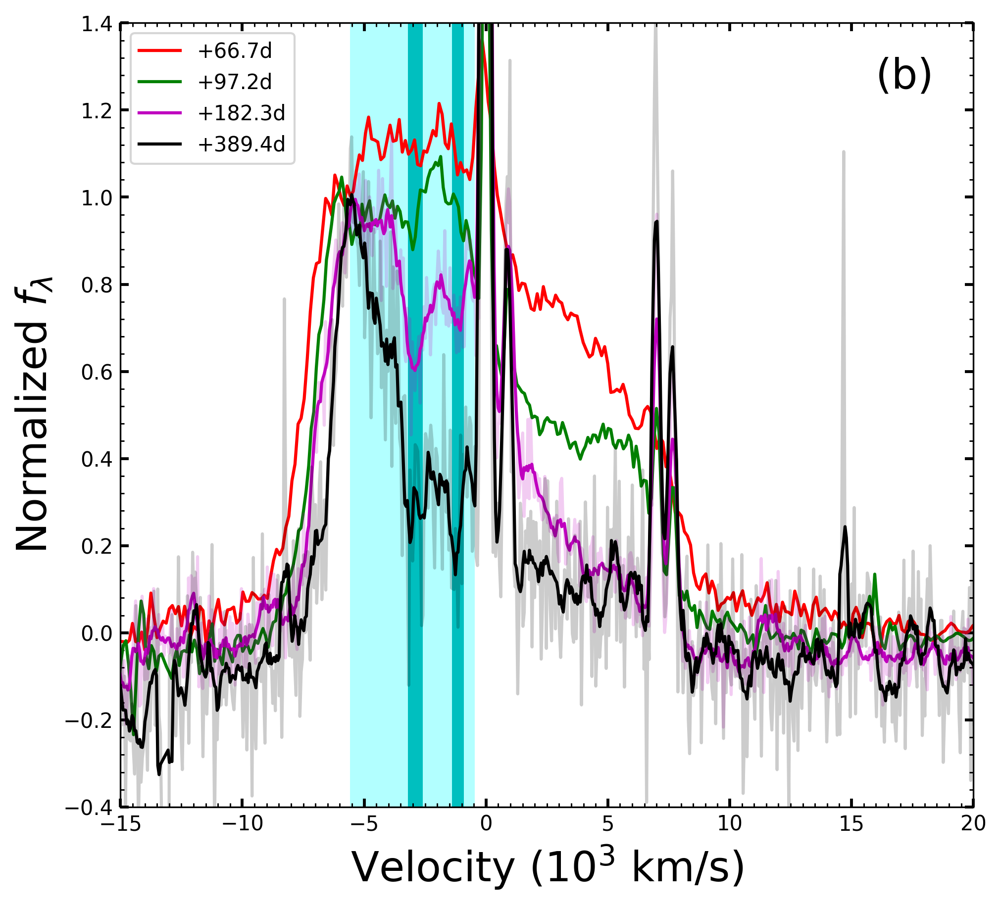
Figure 15: (a) Evolution of the box-like $\rm H\alpha$ emission profile. Phase is coded with colour. All of the spectra are smoothed by a boxcar of suitable width, with the smoothed spectrum superimposed on the original one. Dashed lines denote narrow emission lines from host H ii region. (b) Four of the same spectra, to show the evolution of the CDS component in detail. The broad cyan region denotes the blue side of the CDS component. Two narrow dark-cyan regions mark the troughs in the profiles.

Because both the ionised ejecta and the CDS emit $\rm H\alpha$, to show evolution of the CDS component in detail we select four spectra (+66.7 d, +97.2 d, +182.3 d, and +389.4 d) in Figure 15(a) and replot them in Figure 15(b). The width of the CDS component is only $\sim 5000$ km s^-1, consistent with the prediction that emission lines from the CDS have intermediate width (a few $10^{3}$ km s^-1; Smith 2017). The top of the profile is not very flat and shows many small-scale structures, within which two troughs develop with time. This means clumping exists in the emission region and the clumping gradually becomes severe (Jerkstrand, 2017), probably owing to cooling and increasing of thermal instability (Inserra et al., 2011). Here, however, we cannot determine whether this clumping occurs in the ionised ejecta, the CDS, or both; this question will be answered in Section 7.3.

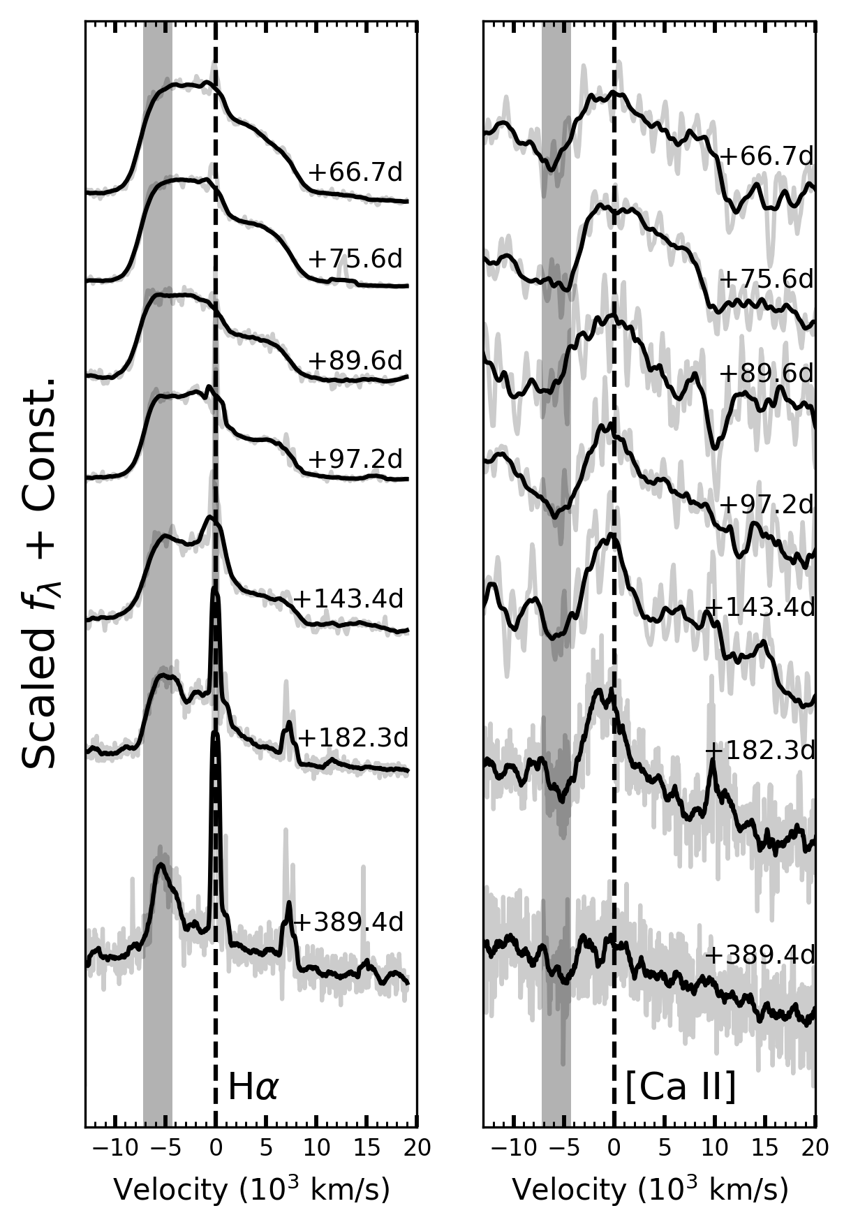
Figure 16: Comparison between evolution of $\rm H\alpha$ emission (left panel) and [Ca ii] $\lambda\lambda$7291, 7323 (right panel). The $\rm H\alpha$ velocity is relative to 6563 Å and the [Ca ii] velocity is relative to 7307 Å. Vertical dashed lines mark zero velocity and shaded regions in both panels denote the velocity between $-7200$ km s^-1 and $-4300$ km s^-1. This shaded region covers the blue minimum of [Ca ii], but not for $\rm H\alpha$, which is located at larger velocity beyond this region. Note that the continuum has not been removed.

Another observed emission line in late-phase spectra is [Ca ii] $\lambda\lambda$7291, 7323. As shown in Figure 16, [Ca ii] also exhibits a box-like shape and broad width, but its BVZI ($-7200$ km s^-1 to $-4300$ km s^-1) is lower than that of $\rm H\alpha$. This intermediate width indicates that [Ca ii] emission is very likely from the CDS, as suggested by Chevalier & Fransson (1994), who argued that it should arise almost exclusively in the CDS. Similarly, [Ca ii] reveals increasing red-blue asymmetry, which can be attributed to dust formation. Compared to $\rm H\alpha$, however, the red side of [Ca ii] emission extends to a larger velocity than its blue side. This could result from very severe scattering, or there exists emission of other elements that we have not identified.

7 Discussion

7.1 When does the CSI begin?

For SN 2018hfm, interaction between the ejecta and CSM is confirmed by several pieces of evidence, including the small bump at the end of the plateau in the light curves, high-velocity features of hydrogen and helium emerging in photospheric spectra, and the box-like $\rm H\alpha$ emission-line profile seen in late-phase spectra. However, when does the interaction actually begin?

The bell-shaped $\rm H\alpha$ profile in the +57.7 d spectrum can be decomposed into a shallow-absorption P Cygni profile and a box-like shape, suggesting that interaction must occur before this time. The small bump emerging in the $V/g$-band light curve suggests the CSI should occur at least by $\sim 40$ d after explosion. However, as shown in Figure 13(b), $\rm H\alpha$ shows abnormal acceleration owing to the influence of CSI. This acceleration begins before +30 d, indicating that the interaction should exist at an even earlier phase. Considering that the outer-layer ejecta have a velocity of $\sim 10,000$ km s^-1, and assuming the interaction occurs at $\sim 30$ d after explosion, we estimate that the CSM is located at a radius of $\sim 2.6\times 10^{15}$ cm ($\sim 170$ au) from the progenitor. Adopting a wind velocity of $\sim 10$ km s^-1, we find that the CSM was produced at $t\approx 80$ yr before the SN explosion.

7.2 Progenitor scenario of SN 2018hfm

Progenitors of many SNe II have been identified as red supergiant (RSG) stars in pre-explosion images (Smartt et al. 2009, and references therein). For SN 2018hfm, despite no images before explosion being found, we can discuss its possible progenitor scenario through characteristics of the SN evolution.

For the light-curve morphology, SN 2018hfm has a luminous peak, a large plateau slope, and a short plateau duration. From modelling the bolometric light curve, we find that SN 2018hfm has a relatively low explosion energy of $\sim 10^{50}$ erg. Considering that the main energy source of the tail-phase light curve is likely from CSI (see Sec.5.5), the mass of ⁵⁶Ni is expected to be very small, or possibly there is no contribution of ⁵⁶Ni at all. These features are reminiscent of the low-energy SN progenitor study of Lisakov et al. (2018). They evolve a single star with an initial mass of 27 $\rm M_{\odot}$ to the pre-SN phase and explode the star with a low energy. They find that this high-mass progenitor tends to retain small mass in its hydrogen envelope before explosion owing to great mass loss during the RSG phase. This low-mass envelope leads to a light curve with a relatively bright peak, fast post-peak decline, and short plateau duration, which is quite similar to the light curve of SN 2018hfm. And in their low-energy explosion model, the entire CO core falls back, and hence no $\rm{}^{56}Ni$ is expelled outside. This is a possible explanation if the tail luminosity of SN 2018hfm is completely supplied by CSI. Moreover, Lisakov et al. (2018) predict in their model that the SN shows a bluer colour at early phases than normal SNe II. They attribute this to the large radius ($>800\,\rm R_{\odot}$) of the pre-SN progenitor, which impacts the cooling from expansion. We observe the bluer colours and we infer that the progenitor of SN 2018hfm has an extended radius ($>1000\,\rm R_{\odot}$). However, the large flux ratio between [Ca ii] and [O i] seen in the late-time spectra suggests that the progenitor mass of SN 2018hfm is not as large as 27 $\rm M_{\odot}$.

Reguitti et al. (2021) describe some observational similarities between low-energy SNe II and electron-capture SNe (ECSNe; Tominaga et al. 2013; Moriya et al. 2014), e.g., low explosion energy and little contribution of ⁵⁶Ni at late phase. ECSNe are believed to be the outcome of super-asymptotic giant branch (super-AGB) stars. According to Pumo et al. (2009), super-AGB stars are those which have an inert core (composed of Ne and O) and an envelope of burning helium and hydrogen. The upper limit of the initial mass for a super-AGB star is about $10\sim 11\,\rm M_{\odot}$, which is at the small end of the SNe II progenitor mass range. These super-AGB stars usually experience thermal pulses, so that some mass of the envelope is ejected into the space; meanwhile, some mass is thrown onto the core. When the core mass goes beyond the Chandrasekhar limit ($\sim 1.37\,\rm M_{\odot}$), electron capture reactions occur and finally lead to a core-collapse explosion. However, compared with normal iron-core-collapse SNe, this class of SNe tend to have relatively low explosion energy ($\sim 10^{50}$ erg). Some features of SN 2018hfm are similar to those of ECSNe, such as the low explosion energy of $\sim 10^{50}$ erg, very low mass of ⁵⁶Ni, possibly low progenitor mass inferred from the large flux ratio between [Ca ii] and [O i], and mass-loss history verified by the CSI signature. However, it is difficult to declare that SN 2018hfm is an ECSN simply based on these plausible lines of evidence.

7.3 Dust formation in the ejecta

To quantify how much dust is formed in SN 2018hfm, we use the tool damocles (Bevan, 2018a; Bevan & Barlow, 2016), which is a Monte Carlo code modelling the influence of dust attenuation/scattering on optical/near-infrared emission lines. We construct a very simple configuration, assuming a shell-like emission region with homologous expansion, with velocity of the inner boundary ($V_{\rm in}$) and outer boundary ($V_{\rm out}$) set to the values listed in Table 11. Between $V_{\rm in}$ and $V_{\rm out}$, the density of emitting material (here hydrogen) follows a smooth radial power-law distribution with an index of 5 (i.e., $\rho\propto V^{-5}$). Assuming that the hydrogen is ionised completely, the emissivity ($i$) is proportional to the square of the density: $i\propto V^{-10}$.

In addition, this emission region is assumed to be optically thin and suffer only dust absorption, without any scattering. The dust is set to be coupled with the emitting material, so that its density follows the same power-law distribution ($\rho_{\rm dust}\propto V^{-5}$). The composition of the dust is presumed as BE amorphous carbon (Zubko et al., 1996), with a grain radius of 0.01 $\mu$m . We vary the dust mass so that the model can fit the observations well. Note that this configuration is only applied to the ionised ejecta; we do not model the emission from the CDS in this work, because the line profile of the CDS component reveals possible severe scattering. Thus, it is difficult for us to determine the dust mass coupled in the CDS through the simple model. As the CDS is usually very thin and has a very low mass compared with the ejecta, we expect that a large amount of dust was not formed in the CDS. In the following discussion, any dust in the CDS is omitted.

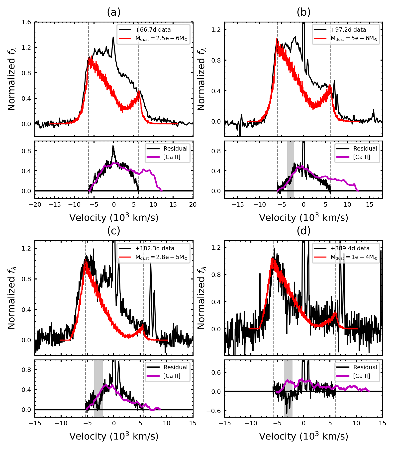
Figure 17: Box-like $\rm H\alpha$ emission lines with the dust model from Bevan & Barlow (2016). We show data and models at four different epochs: (a) +66.7 d, (b) +97.2 d, (c) +182.3 d, and (d) +389.4 d. Black lines in all of the upper panels represent the observed data, while red lines show the model. All models are set to the same parameters except the dust mass as denoted in the label. Residuals of the data after subtracting the model, between two vertical dashed lines, are shown in the lower panels in black lines. The magenta lines superimposed on the residuals are profiles of [Ca ii] $\lambda\lambda$7291, 7323 emission at the same epoch. Grey shaded regions in the lower panels denote the trough in the residual data.

We simulate the $\rm H\alpha$ emission at four epochs (+66.7 d, +97.2 d, +182.3 d, and +389.4 d), which cover the time from the beginning of tail evolution to very late phases. The four emission lines, together with the best-fit model, are presented in the upper panels of Figure 17. For convenience of discussion, we split the $\rm H\alpha$ line profile into three parts according to their left and right shoulders (see vertical dashed lines in Figure 17). For the left part, our model reproduces the data very well, meaning that the assumption of a power-law distribution for the emitting materials is reasonable. In fact, it is exactly the case that outer layers of CCSN progenitors can be mimicked by a steep power law (Chevalier & Fransson, 1994).

For the right part, our model underestimates the data because scattering actually exists in the emission region. Large discrepancies exist in the middle part, where the residuals are shown in the lower panels of Figure 17. These residuals are believed to be caused by the CDS. To verify this idea, we extract [Ca ii] $\lambda\lambda$7291, 7323 emission lines in the same spectra and superimpose them on the residuals after suitable rescaling. One can see that the blue sides of the residuals are consistent with those of [Ca ii] at all of the four selected epochs, which convincingly favours that they are from the same emission region, namely the CDS, as discussed in Section 6.4. The fact that the red side of [Ca ii] extends to a larger velocity than the residuals is probably due to blending with other emission lines. In Section 6.4, we attribute the small troughs on the top of the $\rm H\alpha$ emission profile to clumping in the emission region, but we cannot determine whether the clumping is located in the ionised ejecta or in the CDS. From comparison with the [Ca ii] line profiles, we find the trough exists in the residuals but not in [Ca ii]. Therefore we conclude that the troughs should come from the ionised ejecta.

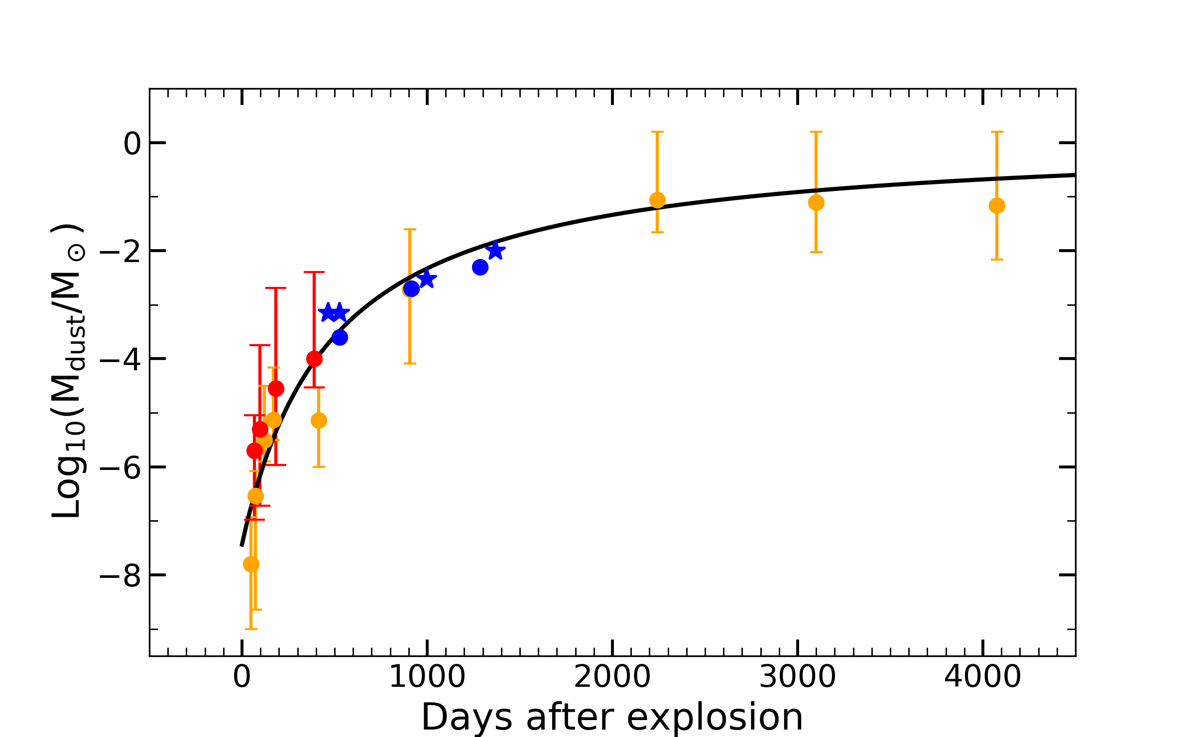
Figure 18: Dust-mass evolution of SN 2018hfm (red circles; this paper), SN 2005ip (orange cicles; Bevan et al. 2019), and SN 2010jl (blue circles and blue stars; Bevan et al. 2020). Circles represent dust mass estimates through the red-blue asymmetry of optical emission lines, while stars represent estimates through fitting the infrared SEDs. The error bars are the 16th and 84th quartiles of the 1D dust-mass posterior distributions (see text). The black line shows the best-fit curve with the form of Eq. 4 proposed by Bevan et al. (2019).

From the models described above, we find that dust is formed continuously as time elapses, from $2.5\times 10^{-6}\,\rm M_{\odot}$ on +66.7 d to $1\times 10^{-4}\,\rm M_{\odot}$ on +389.4 d. To examine the reliability of these dust-mass estimates, we use a Bayesian approach characterised by the application of an affine invariant Markov Chain Monte Carlo ensemble sampler to damocles, to produce marginalised one-dimensional (1D) posterior probability distributions of our input parameters. This method was first used for SN 1987A by Bevan (2018b). We take the 16th and 84th quartiles of the 1D dust-mass posterior distributions as lower and upper limits at each epoch, and find that our dust-mass estimation of SN 2018hfm at all four epochs coincides with the uncertainty ranges between the two limits. As shown in Figure 18, even though the uncertainty ranges are somewhat large (across $\sim 2$ orders of magnitude, possibly owing to the low signal-to-noise ratio of the spectra), it is clear that dust mass is newly formed throughout an interval of $\sim 300$ d, increasing from a relatively low mass range ($10^{-7}$–$10^{-5}\,\rm M_{\odot}$) to a high mass range ($10^{-4}$–$10^{-3}\,\rm M_{\odot}$). Dust formation has been also observed in several other SNe II, such as SN 1987A (Bevan & Barlow, 2016), SN 2005ip (Bevan et al., 2019), and SN 2010jl (Bevan et al., 2020). Bevan et al. (2020) find that the dust-formation rate of these three SNe obeys a best-fit curve with the form

$$-\log_{10}\left(\frac{M_{\rm dust}}{\rm M_{\odot}}\right)=c\left(a\frac{t}{\rm days}+b\right)^{-1}+d,$$ (4)

where $a=0.0076$, $b=3.66$, $c=27.7$, and $d=-0.13$. We present this curve in Figure 18, overplotted with the dust mass measured from SN 2018hfm, SN 2005ip, and SN 2010jl. One can see that the dust-formation rate of SN 2018hfm also follows this curve, indicating that more dust is expected to be produced in this SN at later phases.

8 Conclusions

We present extensive photometric data for SN 2018hfm, covering the rise, plateau-like phase, transitional stage, and tail phase, from which we estimate an explosion date of MJD $=58395.2\pm 5.3$. The $V$-band light curve has a peak of $-18.69\pm 0.64$ mag, followed by a very rapid decline with rate of $\rm s_{2}=4.42\pm 0.13$ mag (100 d)^-1. After about 50 days, the $V$-band light curve abruptly drops by $\sim 3$ mag and then enters the tail phase. From the reconstructed bolometric light curve, we find that the ejecta mass of SN 2018hfm is very low, only $\sim 1.3\,\rm M_{\odot}$. The low tail luminosity indicates a small mass of ⁵⁶Ni ($<0.015\,\rm M_{\odot}$) produced in the explosion, consistent with the low explosion energy ($0.3\times 10^{51}$ erg).

Extensive optical spectra of this SN, spanning from +6.4 d to +389.4 d after explosion, are shown. At very early phases, they are characterised by a blue featureless continuum. Through comparisons with other SNe II, metal lines, such as Ca ii, O i, and Fe ii, are identified in the photospheric spectra. During very late phases, spectra of SN 2018hfm exhibit asymmetric box-like emission-line profiles of $\rm H\alpha$ and [Ca ii] $\lambda\lambda$7291, 7323, which are tightly related to circumstellar interaction and dust formation. Through modelling the line profiles, we estimate the dust mass produced in the ionised ejecta, finding that the dust increases from $\sim 10^{-6}\,\rm M_{\odot}$ at +66.7 d to $10^{-4}$–$10^{-3}\,\rm M_{\odot}$ at +389.4 d. This dust-formation rate follows a curve proposed by Bevan et al. (2019), similar to that of SN 1987A, SN 2005ip, and SN 2010jl.

Based on the observational features and the parameters inferred from the SN data, such as a low mass of ⁵⁶Ni, a low explosion energy, and the mass-loss history, we discuss possible progenitor scenarios of SN 2018hfm. We find that these features link the SN to a possible electron-capture explosion, but an iron-core-collapse SN exploded with low energy can also form most of the observational characteristics.

Data Availability

Photometric data for SN 2018hfm are presented in Table 1, Table 2 and Table 3. Spectroscopic data are available on reasonable request to the corresponding authors.

Appendix A Preprocessing on box-like $\rm H\alpha$ emission

Taking Figure 19 as an example, we describe the preprocessing performed on the box-like $\rm H\alpha$ emission line. First, a straight line was fit to the continuum, as shown in panel (a); it was then subtracted from the profile. We defined a “left roof” on the height of the left top edge (see panel(b)), and divided the profile by this value to normalise the profile. We determined the blue velocity at half maximum (BVHM), blue/red velocity at zero intensity (B/RVZI), inner boundary velocity ($V_{\rm in}$), and “right roof ratio,” shown in the following panels.

Note that in panel (b) of Figure 19, three lines (red, green, and blue) are superimposed on the top of the profile. The blue component is likely from an H ii region in the host galaxy. The green component is believed to be from the cold dense shell (CDS). The red line denotes the left shoulder of the main box-like profile, which is from recombination of the ionised outer ejecta.

The box-like profile is formed from a shell-like emission region. Velocities of its inner boundary ($V_{\rm in}$) and outer boundary ($V_{\rm out}$) are tightly related to the line profile, as shown in panels (d) and (e). The ratio of the right to the left height of the profile is defined as “right roof ratio” in panel (f), which reflects asymmetry of the profile and is related to dust properties.

All of the values of the parameters defined above are listed in Table 11.

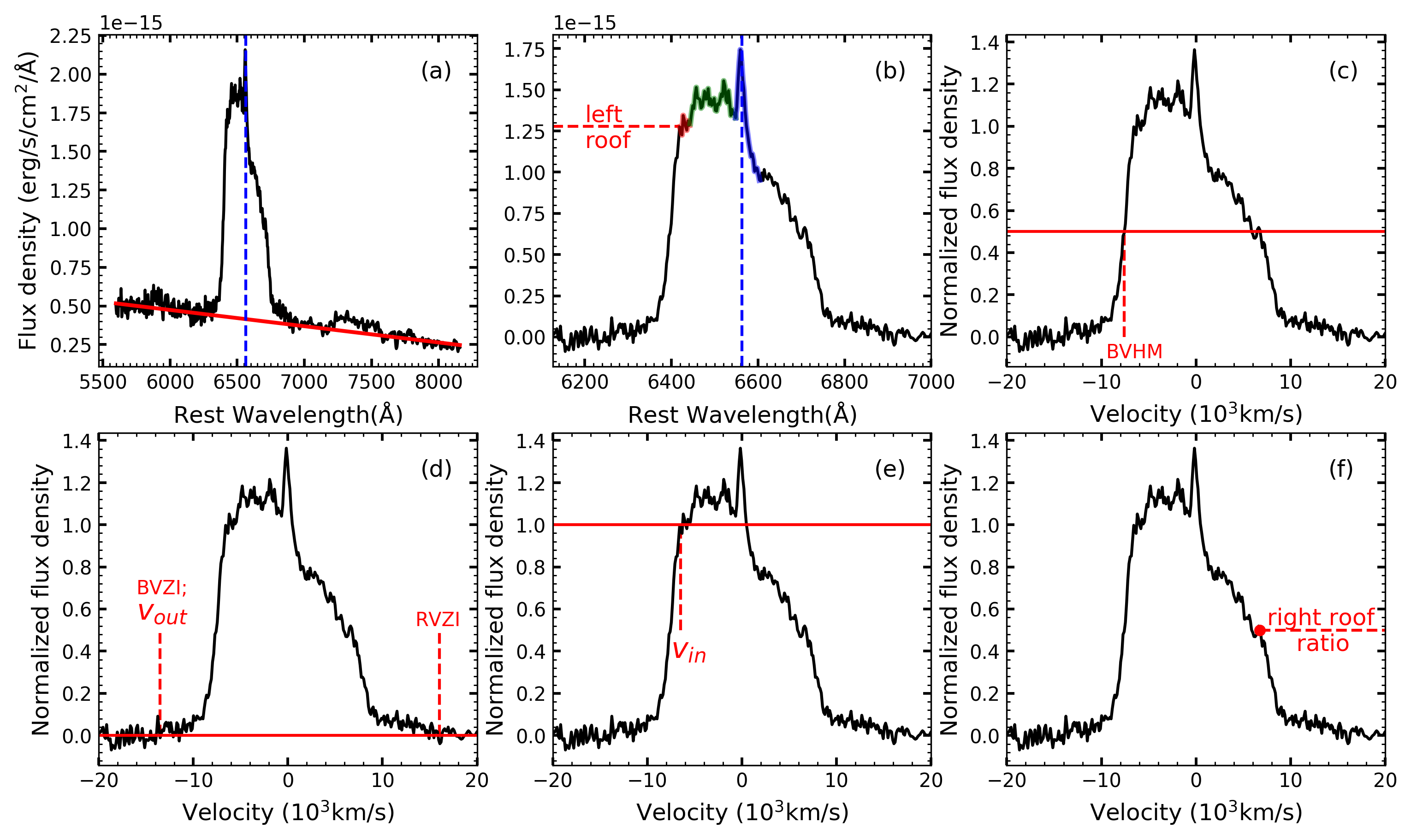
Figure 19: Demonstration of preprocessing the box-like $\rm H\alpha$ emission. For all six panels, black lines are $\rm H\alpha$ emission in the spectrum taken +66.7 d after explosion. (a) The red line is fit to the continuum. The dashed line denotes the location of 6563 Å. (b) The red dashed line defines the “left roof.” Three components of the profile are highlighted by three colour (red, green, blue). The blue dashed line denotes the location of 6563 Å. (c) Definition of BVHM. (d) Definition of BVZI (equal to $V_{\rm out}$) and RVZI. (e) Definition of $V_{\rm in}$. (f) Definition of “right roof ratio.”

References

- Adelman-McCarthy et al. (2008) Adelman-McCarthy J. K., et al., 2008, ApJS, 175, 297
- Anderson et al. (2014) Anderson J. P., et al., 2014, ApJ, 786, 67
- Anderson et al. (2016) Anderson J. P., et al., 2016, A&A, 589, A110
- Andrews et al. (2010) Andrews J. E., et al., 2010, ApJ, 715, 541
- Arnett (1982) Arnett W. D., 1982, ApJ, 253, 785
- Barbon et al. (1982) Barbon R., Ciatti F., Rosino L., 1982, A&A, 116, 35
- Barbon et al. (1990) Barbon R., Benetti S., Cappellaro E., Rosino L., Turatto M., 1990, A&A, 237, 79
- Becker (2015) Becker A., 2015, HOTPANTS: High Order Transform of PSF ANd Template Subtraction (ascl:1504.004)
- Bersten & Hamuy (2009) Bersten M. C., Hamuy M., 2009, ApJ, 701, 200
- Bertoldi et al. (2003) Bertoldi F., Carilli C. L., Cox P., Fan X., Strauss M. A., Beelen A., Omont A., Zylka R., 2003, A&A, 406, L55
- Bevan (2016) Bevan A. M., 2016, PhD thesis, University College London
- Bevan (2018a) Bevan A., 2018a, DAMOCLES: Monte Carlo line radiative transfer code (ascl:1807.023)
- Bevan (2018b) Bevan A., 2018b, MNRAS, 480, 4659
- Bevan & Barlow (2016) Bevan A., Barlow M. J., 2016, MNRAS, 456, 1269
- Bevan et al. (2019) Bevan A., et al., 2019, MNRAS, 485, 5192
- Bevan et al. (2020) Bevan A. M., et al., 2020, ApJ, 894, 111
- Blinnikov (2017) Blinnikov S., 2017, Interacting Supernovae: Spectra and Light Curves. p. 843, doi:10.1007/978-3-319-21846-5_31
- Blondin & Tonry (2011) Blondin S., Tonry J. L., 2011, SNID: Supernova Identification (ascl:1107.001)
- Botticella et al. (2012) Botticella M. T., Smartt S. J., Kennicutt R. C., Cappellaro E., Sereno M., Lee J. C., 2012, A&A, 537, A132
- Bradley et al. (2017) Bradley L., et al., 2017, Astropy/Photutils: V0.4, doi:10.5281/zenodo.1039309
- Buta (1982) Buta R. J., 1982, PASP, 94, 578
- Cardelli et al. (1989) Cardelli J. A., Clayton G. C., Mathis J. S., 1989, ApJ, 345, 245
- Chang et al. (2015) Chang Y.-Y., van der Wel A., da Cunha E., Rix H.-W., 2015, ApJS, 219, 8
- Chevalier & Fransson (1992) Chevalier R. A., Fransson C., 1992, ApJ, 395, 540
- Chevalier & Fransson (1994) Chevalier R. A., Fransson C., 1994, ApJ, 420, 268
- Chugai (1990) Chugai N. N., 1990, Soviet Astronomy Letters, 16, 457
- Chugai et al. (2007) Chugai N. N., Chevalier R. A., Utrobin V. P., 2007, ApJ, 662, 1136
- Collins & Kielkopf (2013) Collins K., Kielkopf J., 2013, AstroImageJ: ImageJ for Astronomy (ascl:1309.001)
- Dessart et al. (2014) Dessart L., et al., 2014, MNRAS, 440, 1856
- Domínguez et al. (2013) Domínguez A., et al., 2013, ApJ, 763, 145
- Elmhamdi et al. (2003) Elmhamdi A., et al., 2003, MNRAS, 338, 939
- Fan et al. (2015) Fan Y.-F., Bai J.-M., Zhang J.-J., Wang C.-J., Chang L., Xin Y.-X., Zhang R.-L., 2015, Research in Astronomy and Astrophysics, 15, 918
- Faran et al. (2014a) Faran T., et al., 2014a, MNRAS, 442, 844
- Faran et al. (2014b) Faran T., et al., 2014b, MNRAS, 445, 554
- Filippenko (1997) Filippenko A. V., 1997, ARA&A, 35, 309
- Gal-Yam (2017) Gal-Yam A., 2017, Observational and Physical Classification of Supernovae. p. 195, doi:10.1007/978-3-319-21846-5_35
- Ganeshalingam et al. (2010) Ganeshalingam M., et al., 2010, ApJS, 190, 418
- Guillochon et al. (2017) Guillochon J., Parrent J., Kelley L. Z., Margutti R., 2017, ApJ, 835, 64
- Gutiérrez et al. (2017) Gutiérrez C. P., et al., 2017, ApJ, 850, 89
- Hiramatsu et al. (2020) Hiramatsu D., et al., 2020, Luminous Type II Short-Plateau Supernovae 2006Y, 2006ai, and 2016egz: A Transitional Class from Stripped Massive Red Supergiants (arXiv:2010.15566)
- Huang et al. (2012) Huang F., Li J.-Z., Wang X.-F., Shang R.-C., Zhang T.-M., Hu J.-Y., Qiu Y.-L., Jiang X.-J., 2012, Research in Astronomy and Astrophysics, 12, 1585
- Huang et al. (2015) Huang F., et al., 2015, ApJ, 807, 59
- Inserra et al. (2011) Inserra C., et al., 2011, MNRAS, 417, 261
- Jerkstrand (2017) Jerkstrand A., 2017, Spectra of Supernovae in the Nebular Phase. p. 795, doi:10.1007/978-3-319-21846-5_29
- Karachentsev & Kaisina (2013) Karachentsev I. D., Kaisina E. I., 2013, AJ, 146, 46
- Kauffmann et al. (2003) Kauffmann G., et al., 2003, MNRAS, 346, 1055
- Kilpatrick et al. (2017) Kilpatrick C. D., et al., 2017, MNRAS, 465, 4650
- Kochanek et al. (2017) Kochanek C. S., et al., 2017, PASP, 129, 104502
- Koleva et al. (2013) Koleva M., Bouchard A., Prugniel P., De Rijcke S., Vauglin I., 2013, MNRAS, 428, 2949
- Kotak et al. (2009) Kotak R., et al., 2009, ApJ, 704, 306
- Kozasa et al. (1991) Kozasa T., Hasegawa H., Nomoto K., 1991, A&A, 249, 474
- Lang et al. (2012) Lang D., Hogg D. W., Mierle K., Blanton M., Roweis S., 2012, Astrometry.net: Astrometric calibration of images (ascl:1208.001)
- Lisakov et al. (2018) Lisakov S. M., Dessart L., Hillier D. J., Waldman R., Livne E., 2018, MNRAS, 473, 3863
- Litvinova & Nadezhin (1985) Litvinova I. Y., Nadezhin D. K., 1985, Soviet Astronomy Letters, 11, 145
- Marano et al. (1980) Marano B., Vettolani P., Zitelli V., Dapergolas A., 1980, IAU Circ., 3542, 1
- Matheson et al. (2000a) Matheson T., et al., 2000a, AJ, 120, 1487
- Matheson et al. (2000b) Matheson T., Filippenko A. V., Ho L. C., Barth A. J., Leonard D. C., 2000b, AJ, 120, 1499
- Meikle et al. (2007) Meikle W. P. S., et al., 2007, ApJ, 665, 608
- Miller & Stone (1993) Miller J., Stone R., 1993, Lick Observatory Technical Reports, pp 66(Santa Cruz, CA: Lick Obs.)
- Moriya et al. (2014) Moriya T. J., Tominaga N., Langer N., Nomoto K., Blinnikov S. I., Sorokina E. I., 2014, A&A, 569, A57
- Morrissey et al. (2007) Morrissey P., et al., 2007, ApJS, 173, 682
- Nagy & Vinkó (2016) Nagy A. P., Vinkó J., 2016, A&A, 589, A53
- Nascimbeni et al. (2018) Nascimbeni V., Granata V., Benetti S., Cappellaro E., Tomasella ., Turatto M., 2018, Transient Name Server Classification Report, 2018-2156, 1
- Oke & Gunn (1983) Oke J. B., Gunn J. E., 1983, ApJ, 266, 713
- Oke et al. (1995) Oke J. B., et al., 1995, PASP, 107, 375
- Olivares E. et al. (2010) Olivares E. F., et al., 2010, ApJ, 715, 833
- Osterbrock (1989) Osterbrock D. E., 1989, Astrophysics of gaseous nebulae and active galactic nuclei
- Pastorello et al. (2006) Pastorello A., et al., 2006, MNRAS, 370, 1752
- Pastorello et al. (2009) Pastorello A., et al., 2009, MNRAS, 394, 2266
- Patat et al. (1995) Patat F., Chugai N., Mazzali P. A., 1995, A&A, 299, 715
- Pettini & Pagel (2004) Pettini M., Pagel B. E. J., 2004, MNRAS, 348, L59
- Poznanski et al. (2012) Poznanski D., Prochaska J. X., Bloom J. S., 2012, MNRAS, 426, 1465
- Pumo et al. (2009) Pumo M. L., et al., 2009, ApJ, 705, L138
- Reguitti et al. (2021) Reguitti A., et al., 2021, MNRAS, 501, 1059
- Richmond et al. (1994) Richmond M. W., Treffers R. R., Filippenko A. V., Paik Y., Leibundgut B., Schulman E., Cox C. V., 1994, AJ, 107, 1022
- Richmond et al. (1996) Richmond M. W., Treffers R. R., Filippenko A. V., Paik Y., 1996, AJ, 112, 732
- Rui et al. (2019) Rui L., et al., 2019, MNRAS, 485, 1990
- Schlegel (1990) Schlegel E. M., 1990, MNRAS, 244, 269
- Schlegel (1996) Schlegel E. M., 1996, AJ, 111, 1660
- Schlegel et al. (1998) Schlegel D. J., Finkbeiner D. P., Davis M., 1998, ApJ, 500, 525
- Shappee et al. (2014) Shappee B. J., et al., 2014, ApJ, 788, 48
- Silverman et al. (2012) Silverman J. M., et al., 2012, MNRAS, 425, 1789
- Singh et al. (2019) Singh A., Kumar B., Moriya T. J., Anupama G. C., Sahu D. K., Brown P. J., Andrews J. E., Smith N., 2019, ApJ, 882, 68
- Smartt et al. (2009) Smartt S. J., Eldridge J. J., Crockett R. M., Maund J. R., 2009, MNRAS, 395, 1409
- Smith (2017) Smith N., 2017, Interacting Supernovae: Types IIn and Ibn. p. 403, doi:10.1007/978-3-319-21846-5_38
- Stahl et al. (2019) Stahl B. E., et al., 2019, MNRAS, 490, 3882
- Stanek (2018) Stanek K. Z., 2018, Transient Name Server Discovery Report, 2018-1539, 1
- Stetson (1987) Stetson P. B., 1987, PASP, 99, 191
- Takáts & Vinkó (2012) Takáts K., Vinkó J., 2012, MNRAS, 419, 2783
- Tominaga et al. (2013) Tominaga N., Blinnikov S. I., Nomoto K., 2013, ApJ, 771, L12
- Turatto et al. (2003) Turatto M., Benetti S., Cappellaro E., 2003, in Hillebrandt W., Leibundgut B., eds, From Twilight to Highlight: The Physics of Supernovae. p. 200 (arXiv:astro-ph/0211219), doi:10.1007/10828549_26
- Valenti et al. (2015) Valenti S., et al., 2015, MNRAS, 448, 2608
- Valenti et al. (2016) Valenti S., et al., 2016, MNRAS, 459, 3939
- Weil et al. (2020) Weil K. E., Fesen R. A., Patnaude D. J., Milisavljevic D., 2020, ApJ, 900, 11
- Woosley & Weaver (1995) Woosley S. E., Weaver T. A., 1995, ApJS, 101, 181
- Yuan et al. (2013) Yuan H. B., Liu X. W., Xiang M. S., 2013, MNRAS, 430, 2188
- Zhang et al. (2006) Zhang T., Wang X., Li W., Zhou X., Ma J., Jiang Z., Chen J., 2006, AJ, 131, 2245
- Zhang et al. (2020) Zhang J., et al., 2020, MNRAS, 498, 84
- Zheng et al. (2018) Zheng W., Brink T., Filippenko A. V., 2018, Transient Name Server Classification Report, 2018-1554, 1
- Zubko et al. (1996) Zubko V. G., Mennella V., Colangeli L., Bussoletti E., 1996, MNRAS, 282, 1321