Constrained Mean Shift for Representation Learning

Abstract

We are interested in representation learning from labeled or unlabeled data. Inspired by recent success of self-supervised learning (SSL), we develop a non-contrastive representation learning method that can exploit additional knowledge. This additional knowledge may come from annotated labels in the supervised setting or an SSL model from another modality in the SSL setting. Our main idea is to generalize the mean-shift algorithm by constraining the search space of nearest neighbors, resulting in semantically purer representations. Our method simply pulls the embedding of an instance closer to its nearest neighbors in a search space that is constrained using the additional knowledge. By leveraging this non-contrastive loss, we show that the supervised ImageNet-1k pretraining with our method results in better transfer performance as compared to the baselines. Further, we demonstrate that our method is relatively robust to label noise. Finally, we show that it is possible to use the noisy constraint across modalities to train self-supervised video models.

1 Introduction

It is a common practice in visual recognition to pretrain a model using cross-entropy loss on some annotated data set (e.g., ImageNet) and then use the learned representations on a downstream task with limited annotated data. We are interested in improving this process by generalizing a recent self-supervised learning (SSL) idea to use other sources of knowledge, e.g., annotation.

Recently, we have seen great progress in self-supervised learning (SSL) methods that learn rich representations from unlabeled data. Such methods are important since they do not rely on manual annotation of data which can be costly, biased, or ambiguous. Hence, SSL representations may perform better than supervised ones in transferring to downstream visual recognition tasks.

Some popular recent SSL methods called “contrastive” assume that in the embedding space, an image should be closer to its own augmentation compared to some other random images He et al. (2020). Some other methods learn representations by clustering images together (Caron et al., 2018) using k-means-like algorithms that contrast between different clusters of images. This contrastive setting has been used in the deep learning community for a long time. Even the standard supervised learning with cross entropy loss maximizes the probability of the correct output while suppressing the probability of the wrong outputs automatically through the normalization in the SoftMax function. This can be seen as a form of contrast between correct and wrong categorization.

A recent SSL method, BYOL (Grill et al., 2020), showed that contrasting against random images is not really necessary and can result in a better performance. Only the augmentations of a single image are pulled closer. A very recent work, MSF (Koohpayegani et al., 2021), has shown that this non-contrastive framework, e.g. BYOL, can be generalized by pulling an image to be closer to not only its augmentations but also its nearest neighbors. This can be seen as a mean-shift algorithm that groups similar images together, but is different from k-means based algorithms as it does not contrast against other groups of images or does not cluster images explicitly.

Our main idea is to design a non-contrastive representation learning method that can utilize other sources of knowledge, e.g., labels. We generalize the MSF method further by constraining the nearest neighbor (NN) search using the additional knowledge. This constraint can help in learning a less noisy grouping of images. For instance, in the supervised setting, when we search for the NNs of the query image to average them, we limit the search space to only the images that share the same label as the query image. Such a simple change makes sure that the NNs are all from the correct semantic category so that we do not pull the query towards images from other categories.

Note that we group only a few NNs ($k$ in our method) from the query’s category together instead of grouping all images together as done in standard cross entropy based learning. We believe this relaxes the learning by not forcing all images of a category to form a cluster or be on the same side of a hyper-plane. Such a relaxation can improve the model when using less robust sources of knowledge, e.g., noisy labels.

Moreover, our method is more general and can use other sources of knowledge for constraining the NN search. For instance, when training SSL models from videos, we use an already trained SSL method on one modality, e.g., RGB, to constrain the NN search on SSL training in a different modality, e.g., Flow.

Our method achieves superior results compared to the baselines in supervised setting with clean and noisy labels as well as self-supervised setting in video.

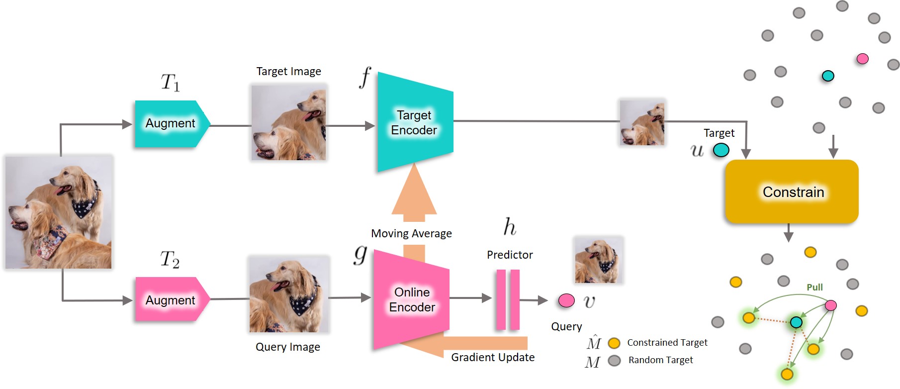
Figure 1: Our method (CMSF): We augment an image twice and pass through online encoder and target encoder followed by $\ell_{2}$ normalization to get $u$ and $v$. We want $v$ to be close to not only $u$, but also the nearest neighbors (NN) of $u$ to perform mean-shift. We constrain the NN pool using some extra knowledge, e.g., image labels, to improve the purity of the NNs. In supervised setting, we use images from the same category only (yellow points) to do NN search. We show that the constrain can come from noisy labels or NN search using a pre-trained SSL embedding on another modality.

2 Method

Similar to MSF (Koohpayegani et al., 2021), given a query image, we are interested in pulling its embedding closer to the mean of the embeddings of its nearest neighbors (NNs). However, unlike MSF, we assume there is another source of knowledge that can constrain the set of data points in which we search for the NNs. This constraint can come from labels in the supervised setting or NNs on another modality in self-supervised learning for multi-modal data, e.g., videos.

To increase the size of the nearest neighbor pool, inspired by He et al. (2020), we use a large queue filled with the most recent training images as the memory bank. We maintain a slowly evolving average of the embedding model similar to He et al. (2020). Note that the computational costs of finding NNs is negligible compared to the overall training cost (Koohpayegani et al., 2021), and they are needed in any method that uses a memory bank, e.g., MoCo (He et al., 2020).

Hence, we assume two embedding networks: a target encoder $f(.)$ with parameters $\theta_{f}$ and an online encoder $g(.)$ with parameters $\theta_{g}$. The online encoder is directly updated using backpropagation while the target encoder is updated as a slowly moving average of the online encoder: $\theta_{f}\leftarrow m\theta_{f}+(1-m)\theta_{g}$ where $m$ is close to $1$. This is the momentum idea introduced in He et al. (2020). We add a predictor head $h(.)$ (Grill et al., 2020) to the end of the online encoder so that pulling the embeddings together encourages one embedding to be predicted by the other one and not necessarily encouraging the two embeddings to be equal. In the experiments, we use a two-layer MLP for $h(.)$.

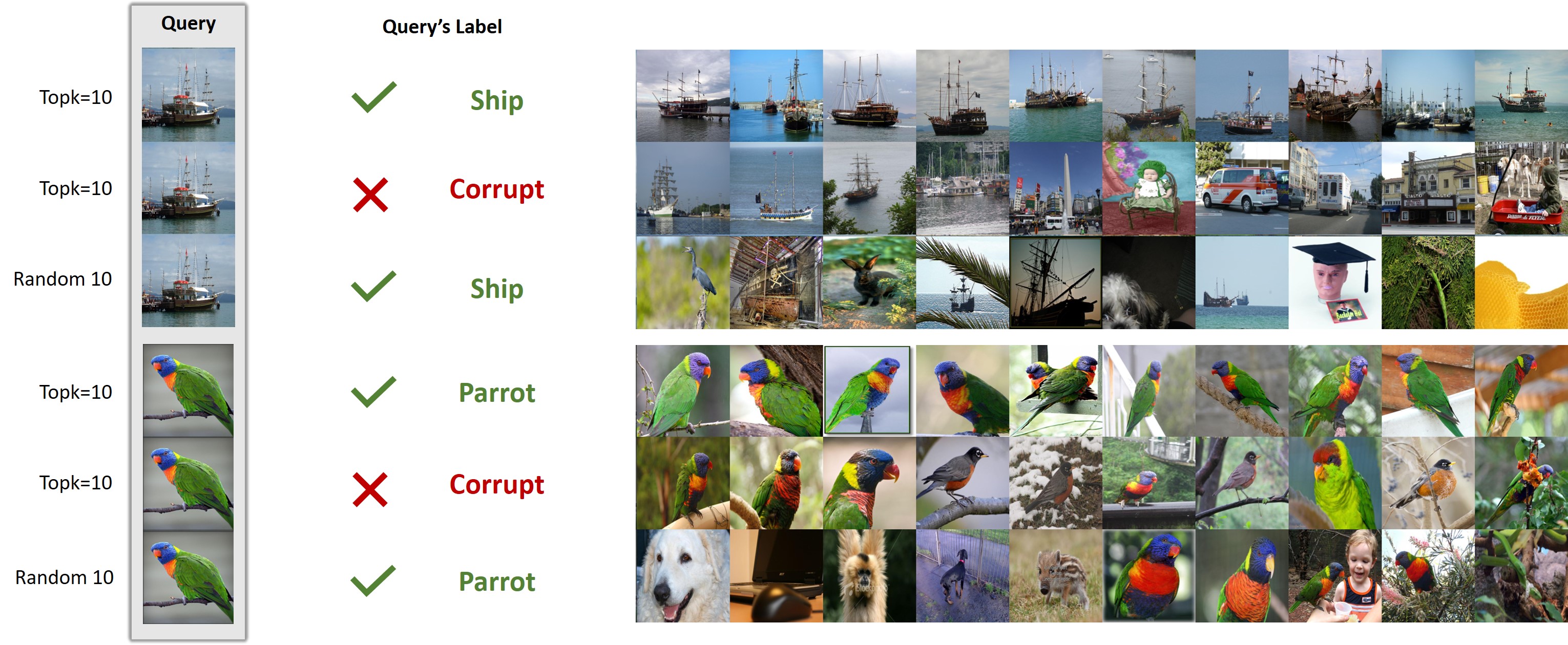
Figure 2: top-$10$ vs. random 10 on ImageNet100 with 50% noisy labels: We show NN search results (sorted from left to right) for a query on the set of images that share the same label with the query. When the query is correctly labeled (Row 1), most NN results are from the same category which is good. When the query is not correctly labeled (Row 2), the few top results are still from the actual category of the query which is good. However, on Row 3, almost half of random results are not from the correct category. This is not surprising, but shows why CMSF with top-$k$ (Rows 1 and 2) performs better than CMSF with top-$all$ and standard cross-entropy supervised learning (Row 3).

Supervised-setting: Given a query image $x$, we augment it twice with $T_{1}(.)$ and $T_{2}(.)$, feed them to the encoders, and normalize them with their $\ell_{2}$ norm to get $u=\frac{f(T_{1}(x))}{||f(T_{1}(x))||_{2}}$ and $v=\frac{h(g(T2(x)))}{||h(g(T2(x)))||_{2}}$. We add $u$ to the memory bank $M$ and remove the oldest entries to maintain a limited size for $M$. Since in the supervised setting, we know the label for each image, we choose the subset of $M$ that shares the same label with the query image to get $\hat{M}$. Then, we find top-$k$ neighbors of $u$ in $\hat{M}$ including $u$ itself and call it $S=\{z_{i}\}_{i=1}^{k}$. Finally, we update $g(.)$ by minimizing the following loss and update $f(.)$ with the momentum update. Note that self-supervised mean-shift algorithm in Koohpayegani et al. (2021) is a specific case of our algorithm in which the constraint does not limit the nearest neighbor search, i,e. $\hat{M}=M$.

$$L=\frac{1}{k}\sum_{i=1}^{k}v^{T}z_{i}$$ (1)

In top-$all$ variation of our method, $k$ is equal to the total size of $\hat{M}$. Note that since $u$ itself is included in the nearest neighbor search, by limiting the size of the constrained set $\hat{M}$ to one (top-$1$), the method will be identical to BYOL (Grill et al., 2020) and by setting $\hat{M}=M$, it will be identical to self-supervised mean-shift (Koohpayegani et al., 2021). Hence, our method covers a larger spectrum by defining the constrained set. Unlike cross-entropy, our method does not encourage collapsing the whole class into one cluster. If the category has a multi-modal distribution, our method may group samples of each mode together without necessarily mixing the modes.

Supervised constraint with noisy labels: Our method in the supervised setting uses the labels to constrain the mean-shift algorithm only rather than enforcing the labels directly in the loss function as done in standard cross-entropy learning. Hence, the constraint does not need to be strictly aligned with the semantic categories. Therefore, our method can benefit even from some weak signal provided by the constraint. For instance, we can use noisy labels to provide the constraint. We do extensive experiments with this setting and show that NNs are key to being robust against noise. Figure 2 shows example NN search results for 50% noisy labeled dataset.

Cross-modal constraint for self-supervised learning: The constraint in our method is not limited to categorical semantic labels as discussed above. We can use nearest neighbor search in another modality to provide the constraint. For instance, in learning rich representations from unlabeled videos, we train a model for the RGB input and use it in a frozen form to constrain the memory bank in training a model for the flow input.

Assuming that $c(.)$ is an already trained embedding for RGB input, we want to train target encoder $f(.)$ and online encoder $g(.)$ for the flow input. Given a query video with RGB component $x_{c}$ and flow component $x$, we calculate $u$ and $v$ similar to the supervised setting using flow models $f(.)$ and $g(.)$ on the flow input $x$, and maintain the flow memory bank $M$ with target embeddings $u$.

Since we do not have labels, we cannot simply construct $\hat{M}$ from $M$ as done in the supervised setting, so we feed the RGB component $x_{c}$ of the video to the frozen $c(.)$ encoder with the same augmentation and normalization to get the embedding $u_{c}$, and maintain a memory bank $M_{c}$ in which the data points follow the same ordering as in $M$. Then, we find $n$ nearest neighbors of $u_{c}$ in $M_{c}$ and use their indices to construct $\hat{M}$ from $M$. Finally, we use $\hat{M}$ to minimize the same loss as in Eq 1 by finding top-$k$ nearest neighbors of $u$ in $\hat{M}$.

Note that we calculate the flow using an unsupervised optical flow algorithm from RGB frames, so RGB and flow are not two distinct modalities as the flow can be calculated from the RGB modality. However, our method does not use this dependency and can be used for two distinct modalities.

2.1 Supervised Setting

2.1.1 Baselines

Cross entropy (Xent): Xent (Baum & Wilczek, 1988; Levin & Fleisher, 1988; Rumelhart et al., 1986) is a popular method for training standard supervised models.

Supervised Contrastive (SupCon): This method extends the instance discrimination framework from self-supervised learning to supervised learning (Khosla et al., 2020). It is a contrastive setting in which the positive set contains all images from the same category. The top-$all$ variation of our method is similar to SupCon without any contrast.

Prototypical Networks (ProtoNW): In order to further study the effect of contrast, we design another contrastive version of our top-$all$ variation. We calculate a prototype for each class by averaging all its instances in the memory bank. Then, similar to prototypical networks (Snell et al., 2017), we compare the input with all prototypes by passing their temperature-scaled cosine distance through a SoftMax layer to get probabilities. Finally, we minimize the cross-entropy loss. Note that this method is still contrastive in nature because of the SoftMax operation.

Frozen Prototype (FrzProto): We randomly initialize a set of prototype embeddings for each class and freeze them throughout training. The prototypes are used as targets for regressing the output embeddings from the backbone network using Cosine similarity loss. This method is very similar to the noise-as-target method (Bojanowski & Joulin, 2017). It can be thought of as the above ProtoNW method but with random class prototypes. Note that since the prototypes are frozen and initialized randomly, even semantically related categories will be far away from each other. Thus, pulling an embedding close to its target class embedding implies that the embedding is pushed away from other class embeddings. This makes the method contrastive. Surprisingly, even frozen prototypes work remarkably well when we change the final linear FC layer to a 2-layer MLP.

Table 1: Linear layer transfer learning evaluation: Our CMSF model with 200 epochs only outperforms all baselines on transfer learning evaluation. We separate supervised and SSL setting. We copied the results for MoCo v2, MSF, and BYOL-asym from Koohpayegani et al. (2021), SimCLR and Xent (1000 epoch) from Chen et al. (2020a), and BYOL from Grill et al. (2020).

Method	Epoch	Food	CIFAR	CIFAR	SUN	Cars	Air-	DTD	Pets	Calt.	Flwr	Mean	Linear
		101	10	100	397	196	craft			101	102	Trans	IN-1k
Xent	200	67.7	89.8	72.5	57.5	43.7	39.8	67.9	91.8	91.1	88.0	71.0	77.2
Xent	90	72.8	91.0	74.0	59.5	56.8	48.4	70.7	92.0	90.8	93.0	74.9	76.2
FrzProto	200	71.8	92.2	75.8	60.8	67.5	58.2	72.2	91.9	93.0	94.2	77.8	75.6
ProtoNW	200	73.3	93.2	78.3	61.5	65.0	57.6	73.7	92.2	94.3	93.7	78.3	76.0
SupCon	200	72.5	93.8	77.7	61.5	64.8	58.6	74.6	92.5	93.6	94.1	78.4	77.5
Xent	1000	72.3	93.6	78.3	61.9	66.7	61.0	74.9	91.5	94.5	94.7	78.9	76.3
CMSF top-$all$	200	73.7	94.2	78.7	62.1	71.7	64.1	73.4	92.5	94.5	95.8	80.1	75.7
CMSF top-$10$	200	74.9	94.4	78.7	62.7	70.8	63.4	73.8	92.2	94.9	95.6	80.1	76.4
MoCo v2	200	70.4	91.0	73.5	57.5	47.7	51.2	73.9	81.3	88.7	91.1	72.6	67.5
SimCLR	1000	72.8	90.5	74.4	60.6	49.3	49.8	75.7	84.6	89.3	92.6	74.0	69.3
MoCo v2	800	72.5	92.2	74.6	59.6	50.5	53.2	74.4	84.6	90.0	90.5	74.2	71.1
BYOL-asym	200	70.2	91.5	74.2	59.0	54.0	52.1	73.4	86.2	90.4	92.1	74.3	69.3
MSF	200	72.3	92.7	76.3	60.2	59.4	56.3	71.7	89.8	90.9	93.7	76.3	72.1
BYOL	1000	75.3	91.3	78.4	62.2	67.8	60.6	75.5	90.4	94.2	96.1	79.2	74.3

2.1.2 Implementation details

We experiment with following augmentations: the augmentation from MoCo-v2 (Chen et al., 2020b) (strong aug), the standard augmentation (std aug) used for supervised Xent ImageNet-1k training (pytorch, ) and weak/strong augmentation from MSF (Koohpayegani et al., 2021). By default both CMSF and SupCon use weak/strong augmentation. All models are trained on supervised ImageNet-1k (IN-1k) for 200 epochs. ResNet-50 (He et al., 2016) is used as the backbone in all experiments. All models are trained with SGD optimizer (lr=0.05, batch size=256, momentum=0.9, and weight decay=1e-4). Unless mentioned, the learning rate scheduler is cosine. The value of momentum for the moving average key encoder in $0.99$ for CMSF and $0.999$ for SupCon. The MLP architecture for CMSF is a sequence of following layers: linear (2048x4096), batch norm, ReLU, and linear (4096x512). The default memory bank size is 128k for CMSF, SupCon, and ProtoNW. For CMSF, top-$k=10$ is the default. For more details see the appendix. Our main CMSF experiment with 200 epochs takes almost 6 days on four NVIDIA-2080TI GPUs.

2.1.3 Evaluation

We evaluate the supervised pre-trained models by treating them as frozen feature extractors and training a single linear layer on top of them for below listed datasets.

Datasets: Unlike Xent, methods like SupCon, ProtoNW, and CMSF do not train a linear classifier during the pre-training stage thus we use the pre-training dataset ImageNet-1k (IN-1k) for evaluating the frozen features. The transfer performance is evaluated on the following datasets: Food101 (Bossard et al., 2014), SUN397 (Xiao et al., 2010), CIFAR10 (Krizhevsky, 2009), CIFAR100 (Krizhevsky, 2009), Cars196 (Krause et al., 2013), Aircraft (Maji et al., 2013), Flowers (Flwrs102) (Nilsback & Zisserman, 2008), Pets (Parkhi et al., 2012), Caltech-101 (Calt101) (Fei-Fei et al., 2004), and DTD (Cimpoi et al., 2014). More details about the datasets like train/val/test split sizes can be found in the supplementary material.

Linear IN-1k: We follow the linear evaluation setup from CompRess (Abbasi Koohpayegani et al., 2020). The features are normalized to have unit $\ell_{2}$ norm and then scaled and shifted to have zero mean and unit variance for each dimension. We use SGD optimizer (lr=0.01, epochs=40, batch size=256, weight decay=1e-4, and momentum=0.9). Learning rate is multiplied by 0.1 at epochs 15 and 30. We use standard supervised ImageNet augmentations (off, ) during training. For Xent and FrzProto, we use the linear classifier trained during pre-training.

Transfer: We follow the procedure outlined in BYOL (Grill et al., 2020) and SimCLR (Chen et al., 2020a) to train a single linear layer on top of the frozen backbone. We tune the hyperparameters for each dataset independently based on the validation set accuracy, and report the final accuracy on the held-out test set. More details about the training procedure can be found in the Appendix.

2.1.4 Results

The results for the IN-1k dataset pre-training are reported in Table 1. First, we find that CMSF has the best transfer evaluation results. Second, as shown by SupCon and Xent (200 epoch version), improvements on the Linear ImageNet-1k evaluation do not always translate to transfer evaluation. Third, methods inspired from SSL like FrzProto, SupCon, and CMSF are generally better than their Xent counterparts for similar number of epochs. Fourth, CMSF is highly competitive with a self-supervised method like BYOL which is trained for 5 times more epochs (200 vs 1000 epochs). Fifth, it is surprising that the FrzProto baseline can achieve such a high performance. Finally, our method performs better at fine-grained datasets, e.g., Cars196 and Aircraft, which we believe is due to preserving multi-modal distribution of the categories.

Table 2: Ablations of baselines and CMSF: All experiments use 200 epochs if not mentioned and use ImageNet-1k dataset. (a) More epochs does not improve transfer accuracy for Xent. Thus, the model available from PyTorch (pytorch, ) (last row) has the best transfer accuracy; (b) We add components of our method to improve SupCon baseline. The baseline implementation of SupCon uses std. aug and 16k memory size and it does not include the target embedding $u$ in the positive set. (c) Using a MLP head improves FrzProto a lot as it allows the post-MLP features to adapt to the regression task, but allows pre-MLP features to be generalizable; (d) We find that our method is not very sensitive to the size of memory bank or in top-$k$; (e) Interestingly, excluding the target embedding $u$ from $\hat{M}$ does not hurts the results. Note that when we do not include the target, the nearest neighbors are still chosen based on the distance to the target, so they will be close to the target. (f) We report the results of our method by with varying the amount of labeled data on ImageNet-1k. We find that only 50% of labeled data is sufficient to reach on-par performance of the fully supervied model. The first row is equivalent to self-supervised MSF, so the numbers are copied from Koohpayegani et al. (2021)

Method	Mean	Linear
	Trans	IN-1k
(a) Xent
lr=$0.05$, cos, epochs=$200$, strong aug.	71.5	77.2
lr=$0.05$, cos, epochs=$200$, std. aug.	71.0	77.3
lr=$0.10$, cos, epochs=$200$, strong aug.	72.3	77.1
lr=$0.05$, cos, epochs=$90$, std. aug.	72.4	76.8
lr=$0.10$, cos, epochs=$90$, std. aug.	74.0	76.7
lr=$0.10$, step, epochs=$90$, std. aug.	74.9	76.2
(b) SupCon
Base SupCon	77.2	77.9
+ change to strong aug.	77.9	77.4
+ add target to positive set	77.8	77.4
+ change to weak/strong aug.	77.8	77.2
+ increase mem size to 128k	78.4	77.5
(c) FrzProto
FC = Linear	43.3	74.0
FC = MLP	77.8	75.6

Method	Mean	Linear
	Trans	IN-1k
(d) CMSF
top-$1$ (BYOL-asym)	74.3	69.3
mem=128k, top-$2$	78.4	76.2
mem=128k, top-$10$	80.1	76.4
mem=128k, top-$20$	79.9	76.3
mem=128k, top-$all$	80.1	75.7
mem=512k, top-$10$	79.9	76.2
mem=512k, top-$20$	80.1	76.3
(e) CMSF
target in top-$10$	80.1	76.4
target not in top-$10$	80.3	76.4
(f) CMSF
labels 0% (MSF)	75.5	72.4
labels 10%	77.8	73.0
labels 20%	78.3	73.8
labels 50%	79.4	75.3
labels 100%	80.1	76.4

2.1.5 Ablations

We explore different design choices and parameters of our method and baselines. We add the techniques used for our methods to the baselines to isolate the effect of different losses. The results are reported in Table 2. Training and evaluation details are the same as in Sections 2.1.2 and 2.1.3.

While traditional semi-supervised learning (Tarvainen & Valpola, 2017) focuses on only improving the performance on the training dataset, we explore how the amount of labeled data in the dataset influences generalization of the representations to other datasets. Since we use the constraint to limit the search space only, our method can easily benefit from the constraint even if it is available only for a subset of the data. Hence, the method can be easily extended to semi-supervised setting by simply setting $\hat{M}=M$ for the unlabeled data. We use two equal-size, separate memory banks for labeled and unlabeled data so that one cannot dominate the whole memory bank. The results are reported in section (f) of Table 2.

2.2 Noisy Supervised Setting

Our method can handle noisy labels since it considers only top NN results as shown in Figure 2. To add noise to the dataset, the labels for a certain percentage of images are corrupted randomly and kept constant throughout training. We consider, 5%, 10%, 25% and 50% label corruption (noise) rates. The corrupted labels are provided in the code (supplementary). For faster experiments, we use the supervised ImageNet-100 (IN-100) split (Tian et al., 2019). Our main goal is to show that top-$k$ is more robust than top-$all$.

Training and evaluation details: The implementation and evaluation details are the same as in Sections 2.1.2 and 2.1.3 except that we use 500 epochs following LooC (Xiao et al., 2020), and use linear evaluation on clean IN-100 for both our method and the baseline. We use a memory bank of size 64k. We observed that the transfer accuracy of Xent on 25% and 50% degrades with longer training, so we report Xent results with 100 epochs only for the corrupted data.

Results: The results are reported in the Figure 3. We observe that by increasing the amount of noise, the accuracy of our method drops less compared to the baseline. The gap is larger for the transfer learning evaluation. Moreover, CMSF top-$all$ degrades more compared to top-$10$. This shows that in the presence of a noisy constraint, it is better to only pull locally close embeddings close together. Since all embeddings of the same class are not guaranteed to contain the same semantic content, doing top-$all$ pulls semantically unrelated embeddings close together which hurts the quality of representations. This is shown in Figure 2.

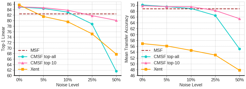
Figure 3: Noisy supervised setting on ImageNet-100: Our method is more robust to noisy annotation compared to Xent. Also, using top-$all$ results in degradation since all images from a single category are not guaranteed to be semantically related. Mean Transfer Accuracy is average accuracy of each model over 10 transfer dataset in our settings.

2.3 Cross-modal Constraint

In the previous Section 2.2 we showed that our method (CMSF with top-$k$) is robust when the constraint is noisy. Here, we explore another such noisy constraint: an already trained SSL model in another modality. Following Han et al. (2021), we use split-1 of UCF-101 (Soomro et al., 2012) (13k videos) as the unlabeled dataset. We use similar augmentation and pre-processing as Han et al. (2021) and calculate optical-flow using unsupervised TV-L1 (Zach et al., 2007) algorithm. We first train two SSL models on RGB and Flow modalities separately using InfoNCE method (van den Oord et al., 2018; Han et al., 2021). Then we continue training on one modality while freezing the other modality and using it as a constraint. In training the flow network using RGB network as constraint, we sample $n$ nearest neighbors in RGB’s memory bank and then we search for top-$k$ nearest neighbors among those samples in Flow’s memory bank. We use the code from Han et al. (2021) for linear evaluation. We report top-1 accuracy for linear classification and recall@1 for retrieval on the extracted features of frozen networks.

Results: We show the results in Table 3. All experiments use spatio-temporal 3D data either in RGB or flow format. Our method outperforms all the baselines including CoCLR (Han et al., 2021) in Flow and is 3.6 points less accurate that CoCLR on RGB modality.

Table 3: Cross-modal constraint: We continue training each SSL model for 200 epochs using MSF (Koohpayegani et al., 2021) for a fair comparison. “Init” column shows what model has been used to initialize the training while “Conatraint” column shows what model is used to provide the constraint. Note that CoCLR (Han et al., 2021) also uses another modality as a constrain in the form of contrastive learning. Rows [1-4] are copied from Han et al. (2021).

Index	Model	Modality	Init	Constraint	Epochs	R@1	Linear
1	Sup Xent	RGB	-	-	-	73.5	77.0
2	Sup UberNCE	RGB	-	-	-	71.6	78.0
3	CoCLRk=5	RGB	-	Flow	500	51.8	70.2
4	CoCLR k=5	Flow	-	RGB	500	48.4	67.8
5	InfoNCE	RGB	-	-	400	35.5	47.9
6	MSF k=5	RGB	5	-	+200	39.6	50.8
7	CMSF n=10, k=5	RGB	5	10	+100	45.8	58.1
8	CMSF n=10, k=5	RGB	5	14	+100	46.2	58.1
9	CoCLR k=5	RGB	5	10	+100	49.8	61.0
10	InfoNCE	Flow	-	-	400	45.3	66.1
11	MSF k=5	Flow	10	-	+200	47.3	64.7
12	CoCLR k=5	Flow	10	9	+100	50.0	67.3
13	CMSF n=10, k=5	Flow	10	9	+100	54.1	71.2
14	CMSF n=10, k=5	Flow	10	5	+100	55.6	70.2

Ablation (effect of $n$): We show the effect of $n$ in Table 5. It is interesting that the 6th row is better than the 4th row. We hypothesize increasing $n$ helps when the constraint is not very accurate (RGB in this case) by loosening the constraint. This is aligned with our intuition.

Implementation Details. For cross-modal experiments, we use S3D (Xie et al., 2018) architecture with the input size of 128 pixels. We initialize from the pretrained weights of InfoNCE (400-epoch) released by (Han et al., 2021). We use following settings for our method: memory bank of size $8,192$, $n=10$, $k=5$, batch size $128$, weight decay $1e-5$, initial lr of $0.001$, and learning rate decay by factor of $10$ at epoch 80. We train each modality for additional 100 epochs using PyTorch Adam optimizer. For a fair comparison, we run CoCLR using their official code by initializing it from the same model as ours.

2.4 Constraining with 2D SSL models

We show that self-supervised 2D ResNet50 model pretrained on ImageNet-1k can be used as a constraint for 3D video SSL models. We initialize S3D backbone from the self-supervised InfoNCE model and continue training it with ImageNet-1k pretrained, SSL ResNet50 as the constraint. We randomly select one frame of input video and feed it to the ResNet50 backbone to get the features for the constraint. We use $n=10$ and $k=5$. We also evaluate the 2D backbone on the center frame of the video only. The results are shown in Table 5. Interestingly, our CMSF Flow model outperforms the 2D model by $3.2$ points in R@1 and $1.7$ point in Linear evaluation. Again since $n>k$, the NN search on the 3D model can search for the best samples rather than fully relying on the constraint.

Implementation Details. We use the same details as the cross-modal experiments except that the initial lr is $0.002$ with decaying by a factor of $10$ at epoch 180.

Table 4: Ablation for the effect of n for cross-modal setting: By comparing Rows 4 and 6, we can see that using $n>k$ helps the model when the constraint is less accurate (more noisy).

Idx	Model	Mod-	Init	Cons-	Epochs	R@1	Linear
		ality		traint
1	InfoNCE	RGB	-	-	400	35.5	47.9
2	InfoNCE	Flow	-	-	400	45.3	66.1
3	CMSF n=5, k=5	RGB	1	2	+100	46.8	59.1
4	CMSF n=5, k=5	Flow	2	3	+100	53.2	70.1
5	CMSF n=10, k=5	RGB	1	2	+100	45.8	58.1
6	CMSF n=10, k=5	Flow	2	5	+100	54.1	71.2
7	CMSF n=20, k=5	RGB	1	2	+100	46.2	58.0
8	CMSF n=20, k=5	Flow	2	7	+100	54.0	70.2

Table 5: Constraining with 2D SSL models: Our method can benefit from constraints that come from an SSL 2D model trained on ImageNet-1k. “CF” refers to running the 2D model on the center frame of the video.

Idx	Model	Arch	Mod-	Cons-	R@1	Linear
			ality	traint
1	2D-MSF	R50	RGB CF	-	57.2	71.5
2	CMSF	S3D	RGB	1	48.9	59.1
3	CMSF	S3D	Flow	1	60.4	73.2

3 Related Work

Supervised learning: Cross-entropy is a well known loss function for supervised learning (Baum & Wilczek, 1988; Levin & Fleisher, 1988; Rumelhart et al., 1986). Cross-entropy is contrastive in nature since ground truth probability of each class is either $0$ or $1$. One drawback of Cross-entropy is its lack of robustness to noisy labels (Zhang & Sabuncu, 2018; Sukhbaatar et al., 2015). Szegedy et al. (2015); Müller et al. (2020) address the issue of hard labeling (one-hot labels) with label smoothing, Hinton et al. (2015); Bagherinezhad et al. (2018); Furlanello et al. (2018) replace hard labels with prediction of pretrained teacher, and Zhang et al. (2018); Yun et al. (2019) propose an augmentation strategy to train on combination of instances and their labels. Another line of works (Goldberger et al., 2004; Salakhutdinov & Hinton, 2007) have attempted to learn representations with good kNN performance. Supervised Contrastive Learning (SupCon) (Khosla et al., 2020) and Wu et al. (2018) improve upon Goldberger et al. (2004) by changing the distance to inner product on $\ell_{2}$ normalized embeddings. Our method is different as it does not use negative samples which makes it non-contrastive. Moreover, we focus on learning transferable representations instead of just focusing on the pretraining task. We also show that our method is robust to noisy supervision.

Constrained clustering: Constrained clustering has been studied before Basu et al. (2008); Legendre (1987); Gançarski et al. (2020). Zhang et al. (2019) adds various constraints to deep k-means-like clustering. Jia et al. (2020) uses constraints with Graph-Laplacian PCA. Anand et al. (2013) generalizes mean-shift algorithm with kernel learning and pairwise constraints. Our method is a simple non-contrastive mean-shift algorithm that is inspired by the recent success in self supervised learning literature by comparing different augmentations of the same image.

Metric learning: The goal of metric learning is to train a representation that puts two instances close in the embedding space if they are semantically close. Two important methods in metric learning are: triplet loss (Chopra et al., 2005; Weinberger et al., 2006; Schroff et al., 2015) and contrastive loss (Sohn, 2016; Bromley et al., 1993). Both use positive and negative samples, but the number of negatives is larger in contrastive losses. Because of the negative samples, these losses are contrastive in nature. It has been shown that metric learning methods perform well on tasks like image retrieval (Wu et al., 2017) and few-shot learning (Vinyals et al., 2017; Snell et al., 2017). One of these few-shot learning works is prototypical networks (Snell et al., 2017) which is similar to a contrastive version of our method with top-$all$.

Self-supervised learning (SSL): Here, we want to learn representations without any annotations. One way to learn form unlabeled data is by solving a pretext task. Examples of a pretext task are colorization (Zhang et al., 2016), jigsaw puzzle (Noroozi & Favaro, 2016), counting (Noroozi et al., 2017) and rotation prediction (Gidaris et al., 2018). Another class of SSL methods are based on instance discrimination (Dosovitskiy et al., 2014). The idea is to classify each image as its own class. Some methods adopted the idea of contrastive learning for instance discrimination (He et al., 2020; Chen et al., 2020a; Caron et al., 2018; 2021). BYOL (Grill et al., 2020) proposes a non-contrastive approach by removing the negative set from contrastive SSL methods and simply regressing target view of an image from the query view. MSF (Koohpayegani et al., 2021) generalizes BYOL by regressing target view and its NNs. Our idea is adopted from MSF (Koohpayegani et al., 2021) by using an additional source of knowledge to constrain the NN search space for the target view.

Multi-modal self-supervised learning. Similar to self-supervised learning on single modality, the goal is to learn a rich representation with more than one modality per instance. One approach is to use corresponding (audio, frame) pairs (Alwassel et al., 2020; Arandjelović & Zisserman, 2017; 2018; Korbar et al., 2018; Patrick et al., 2020; Piergiovanni et al., 2020) with contrastive loss. Another approach is to use video and text narration (Miech et al., 2020).

We adopt the idea of co-training from (Blum & Mitchell, 2000) and CoCLR (Han et al., 2021) where two networks help in training each other. In our case, we train two SSL models in Flow and RGB modalities. We use knowledge of one modality as a constrain to train the other modality.

4 Conclusion

Adopting ideas from SSL literature, we introduce a non-contrastive generalized framework that learns rich representations by grouping similar images together while taking advantage of some other source of knowledge if available, e.g., labels or another modality. We show that our method outperforms the baselines on various settings including supervised with clean or noisy labels, and video SSL settings.

Ethics Statement: We are introducing a method for a core problem in computer vision: representation learning. Hence, similar to most other AI algorithms, our method can be exploited by adversaries for unethical applications. Since we are not focusing on a particular application, we cannot list any specific ethical issues. On the positive note, since our method can achieve similar results with fewer or noisy labeled data, it may facilitate making AI more accessible to a large community leading to democratizing AI.

Reproducibility Statement: To make our work reproducible, we report details of the implementation for each section. For Supervised section, details of implementation are in Section 2.1.2. Details of transfer learning benchmark are in Appendix Section A.3. More implementation details of each baseline are in Appendix Section A.1. Moreover, we submit our code as supplementary material.

Acknowledgment: This material is based upon work partially supported by the United States Air Force under Contract No. FA8750‐19‐C‐0098, funding from SAP SE, and also NSF grant numbers 1845216 and 1920079. Any opinions, findings, and conclusions or recommendations expressed in this material are those of the authors and do not necessarily reflect the views of the United States Air Force, DARPA, or other funding agencies.

Appendix A Appendix

A.1 Implementation Details of Baselines (Section 2.1.1)

The MLP architecture for FrzProto is: linear (2048x2048), batch norm, ReLU, and linear (2048x2048). For SupCon baseline, it is: linear (2048x2048), batch norm, ReLU, and linear (2048x128). For FrzProto, the class prototype embeddings are a matrix of size 1000x2048 for ImageNet-1k. For optimizing SupCon baseline, following [31], we use the first 10 epochs for learning-rate warmup. For both SupCon and ProtoNW, the temperature is $0.1$.

A.2 Semi-Supervised Setting (Section 2.1.5)

In training, we have two memory banks of size 128K each. All samples of a mini-batch are pushed to the unlabeled memory bank while only labeled samples are pushed to the labeled memory bank. Unconstrained loss (Self-Supervised MSF) or constrained loss (Supervised) is calculated for each sample depending on the existence of its label, and the final loss is the mean of losses for the whole mini-batch. All other implementation details are the same as in Section 2.1.2. We report the extended version of Table 2(f) for all 10 transfer dataset. Results are in Table A1.

Table A1: Semi-supervised representation learning with CMSF. We report the results of our method by with varying the amount of labeled data on ImageNet-1k. We find that only 50% of labeled data is sufficient to reach on-par performance of the fully supervied model. The first row is equivalent to self-supervised MSF, so the numbers are copied from Koohpayegani et al. (2021)

Labeled	Food	CIFAR	CIFAR	SUN	Cars	Air-	DTD	Pets	Calt.	Flwr	Mean	Linear
Split	101	10	100	397	196	craft			101	102	Trans
0%	71.2	92.6	76.3	59.2	55.6	53.7	73.2	88.7	92.7	92.0	75.5	72.4
10%	71.6	93.6	78.1	61.0	62.0	59.2	73.4	91.5	93.1	94.4	77.8	73.0
20%	73.3	93.2	77.8	61.3	64.5	60.1	73.6	91.0	93.4	95.0	78.3	73.8
50%	74.1	93.8	79.4	62.1	68.6	63.1	73.0	91.6	93.5	95.0	79.4	75.3
100%	74.9	94.4	78.7	62.7	70.8	63.4	73.8	92.2	94.9	95.6	80.1	76.4

A.3 Implementation Details of Transfer Evaluation (Section 2.1.3)

We use the LBFGS optimizer (max_iter=20, and history_size=10) along with the Optuna library (Akiba et al., 2019) in the Ray hyperparameter tuning framework (Liaw et al., 2018). Each dataset gets a budget of 200 trials to pick the best parameters on validation set. The final accuracy is reported on a held-out test set by training the model on the train+val split using the best hyperparameters. The hyperparameters and their search spaces (in loguniform) are as follows: iterations $\in[0,10^{3}]$, lr $\in[10^{-6},1]$, and weight decay $\in[10^{-9},1]$. We also show that we can reproduce the transfer results for BYOL (Grill et al., 2020) and SimCLR (Chen et al., 2020a) with our framework. The features are extracted with the following pre-processing for all datasets: resize shorter side to 256, take a center crop of size 224, and normalize with ImageNet statistics. No training time augmentation was used.

Table A2: Transfer dataset details: Train, val, and test splits of the transfer datasets are listed in this table. Test split: We follow the details in [32]. For Aircraft, DTD, and Flowers datasets, we use the provided test sets. For Sun397, Cars, CIFAR-10, CIFAR-100, Food101, and Pets datasets, we use the provided val set as the hold-out test set. For Caltech-101, 30 random images per category are used as the hold-out test set. Val split: For DTD and Flowers, we use the provided val sets. For other datasets, the val set is randomly sampled from the train set. For transfer setup, to be close to BYOL [25], the following val set splitting strategies have been used for each dataset: Aircraft: 20% samples per class. Caltech-101: 5 samples per class. Cars: 20% samples per class. CIFAR-100: 50 samples per class. CIFAR-10: 50 samples per class. Food101: 75 samples per class. Pets: 20 samples per class. Sun397: 10 samples per class.

Dataset	Classes	Train samples	Val samples	Test samples	Accuracy measure	Test provided
Food101 [11]	101	68175	7575	25250	Top-1 accuracy	-
CIFAR-10 [35]	10	49500	500	10000	Top-1 accuracy	-
CIFAR-100 [35]	100	45000	5000	10000	Top-1 accuracy	-
Sun397 (split 1) [65]	397	15880	3970	19850	Top-1 accuracy	-
Cars [34]	196	6509	1635	8041	Top-1 accuracy	-
Aircraft [39]	100	5367	1300	3333	Mean per-class accuracy	Yes
DTD (split 1) [18]	47	1880	1880	1880	Top-1 accuracy	Yes
Pets [47]	37	2940	740	3669	Mean per-class accuracy	-
Caltech-101 [20]	101	2550	510	6084	Mean per-class accuracy	-
Flowers [42]	102	1020	1020	6149	Mean per-class accuracy	Yes

A.4 Detailed results for noisy supervised setting (Section 2.2)

Table A3: Noisy supervised setting on ImageNet-100: Our method is more robust to noisy annotation compared to Xent. Also, using top-$all$ results in degradation since all images from a single category are not guaranteed to be semantically related.

Method	Noise	Food	CIFAR	CIFAR	SUN	Cars	Air-	DTD	Pets	Calt.	Flwr	Mean	Linear
		101	10	100	397	196	craft			101	102	Trans	IN-100
Xent	0%	53.6	81.9	61.1	37.8	25.7	29.5	56.9	69.7	70.2	82.3	56.9	85.7
CMSF top-$all$	0%	61.6	88.2	68.5	49.9	54.6	52.7	64.7	82.2	89.6	89.1	70.1	84.9
CMSF top-$10$	0%	62.6	86.8	66.2	50.5	54.7	51.0	64.6	82.4	88.5	90.4	69.8	85.0
Xent	5%	46.5	81.1	58.1	35.8	27.5	36.0	58.7	67.5	73.3	77.0	56.1	81.5
CMSF top-$all$	5%	60.3	87.5	66.4	49.1	55.5	53.0	64.8	80.9	87.3	89.9	69.5	84.4
CMSF top-$10$	5%	61.6	86.8	67.4	49.6	55.8	51.2	63.4	81.5	86.7	90.6	69.5	84.7
Xent	10%	44.1	79.5	56.1	32.4	26.1	34.5	56.1	69.7	72.5	75.1	54.6	79.6
CMSF top-$all$	10%	59.4	86.4	66.0	48.8	55.0	51.4	64.7	80.1	87.8	89.0	68.9	83.1
CMSF top-$10$	10%	60.9	87.2	66.9	49.4	54.2	51.4	65.5	80.6	88.5	90.0	69.5	83.8
Xent	25%	49.0	77.2	54.5	30.6	25.9	30.7	53.1	66.6	64.1	77.8	53.0	75.2
CMSF top-$all$	25%	56.4	85.7	64.2	46.0	53.6	49.6	62.7	74.2	85.2	87.4	66.5	78.8
CMSF top-$10$	25%	58.9	85.2	64.9	47.8	55.0	50.6	64.0	80.0	86.3	89.7	68.2	81.8
Xent	50%	44.4	72.3	51.3	31.1	21.4	24.9	46.0	57.4	56.0	73.0	47.8	67.8
CMSF top-$all$	50%	44.7	79.3	54.9	35.2	35.7	41.2	54.9	54.6	75.3	75.1	55.1	61.6
CMSF top-$10$	50%	58.7	85.7	64.2	47.5	51.6	50.5	62.0	77.3	86.8	70.1	65.4	80.1

References

- (1) Official pytorch supervised imagenet training code. https://github.com/pytorch/examples/blob/master/imagenet/main.py.
- Abbasi Koohpayegani et al. (2020) Soroush Abbasi Koohpayegani, Ajinkya Tejankar, and Hamed Pirsiavash. Compress: Self-supervised learning by compressing representations. Advances in Neural Information Processing Systems, 33, 2020.
- Akiba et al. (2019) Takuya Akiba, Shotaro Sano, Toshihiko Yanase, Takeru Ohta, and Masanori Koyama. Optuna: A next-generation hyperparameter optimization framework. In Proceedings of the 25th ACM SIGKDD international conference on knowledge discovery & data mining, pp. 2623–2631, 2019.
- Alwassel et al. (2020) Humam Alwassel, Dhruv Mahajan, Bruno Korbar, Lorenzo Torresani, Bernard Ghanem, and Du Tran. Self-supervised learning by cross-modal audio-video clustering, 2020.
- Anand et al. (2013) Saket Anand, Sushil Mittal, Oncel Tuzel, and Peter Meer. Semi-supervised kernel mean shift clustering. IEEE transactions on pattern analysis and machine intelligence, 36(6):1201–1215, 2013.
- Arandjelović & Zisserman (2017) Relja Arandjelović and Andrew Zisserman. Look, listen and learn, 2017.
- Arandjelović & Zisserman (2018) Relja Arandjelović and Andrew Zisserman. Objects that sound, 2018.
- Bagherinezhad et al. (2018) Hessam Bagherinezhad, Maxwell Horton, Mohammad Rastegari, and Ali Farhadi. Label refinery: Improving imagenet classification through label progression. arXiv preprint arXiv:1805.02641, 2018.
- Basu et al. (2008) Sugato Basu, Ian Davidson, and Kiri Wagstaff. Constrained clustering: Advances in algorithms, theory, and applications. CRC Press, 2008.
- Baum & Wilczek (1988) Eric Baum and Frank Wilczek. Supervised learning of probability distributions by neural networks. In D. Anderson (ed.), Neural Information Processing Systems. American Institute of Physics, 1988. URL https://proceedings.neurips.cc/paper/1987/file/eccbc87e4b5ce2fe28308fd9f2a7baf3-Paper.pdf.
- Blum & Mitchell (2000) Avrim Blum and Tom Mitchell. Combining labeled and unlabeled data with co-training. Proceedings of the Annual ACM Conference on Computational Learning Theory, 10 2000. doi: 10.1145/279943.279962.
- Bojanowski & Joulin (2017) Piotr Bojanowski and Armand Joulin. Unsupervised learning by predicting noise. In Proceedings of the 34th International Conference on Machine Learning-Volume 70, pp. 517–526. JMLR. org, 2017.
- Bossard et al. (2014) Lukas Bossard, Matthieu Guillaumin, and Luc Van Gool. Food-101 – mining discriminative components with random forests. In European Conference on Computer Vision, 2014.
- Bromley et al. (1993) Jane Bromley, Isabelle Guyon, Yann LeCun, Eduard Säckinger, and Roopak Shah. Signature verification using a” siamese” time delay neural network. Advances in neural information processing systems, 6:737–744, 1993.
- Caron et al. (2018) Mathilde Caron, Piotr Bojanowski, Armand Joulin, and Matthijs Douze. Deep clustering for unsupervised learning of visual features. In Proceedings of the European Conference on Computer Vision (ECCV), pp. 132–149, 2018.
- Caron et al. (2021) Mathilde Caron, Ishan Misra, Julien Mairal, Priya Goyal, Piotr Bojanowski, and Armand Joulin. Unsupervised learning of visual features by contrasting cluster assignments, 2021.
- Chen et al. (2020a) Ting Chen, Simon Kornblith, Mohammad Norouzi, and Geoffrey Hinton. A simple framework for contrastive learning of visual representations. arXiv preprint arXiv:2002.05709, 2020a.
- Chen et al. (2020b) Xinlei Chen, Haoqi Fan, Ross Girshick, and Kaiming He. Improved baselines with momentum contrastive learning. arXiv preprint arXiv:2003.04297, 2020b.
- Chopra et al. (2005) Sumit Chopra, Raia Hadsell, and Yann LeCun. Learning a similarity metric discriminatively, with application to face verification. In 2005 IEEE Computer Society Conference on Computer Vision and Pattern Recognition (CVPR’05), volume 1, pp. 539–546. IEEE, 2005.
- Cimpoi et al. (2014) Mircea Cimpoi, Subhransu Maji, Iasonas Kokkinos, Sammy Mohamed, and Andrea Vedaldi. Describing textures in the wild. In Computer Vision and Pattern Recognition, 2014.
- Dosovitskiy et al. (2014) Alexey Dosovitskiy, Jost Tobias Springenberg, Martin Riedmiller, and Thomas Brox. Discriminative unsupervised feature learning with convolutional neural networks. In Advances in neural information processing systems, pp. 766–774, 2014.
- Fei-Fei et al. (2004) Li Fei-Fei, Rob Fergus, and Pietro Perona. Learning generative visual models from few training examples: An incremental bayesian approach tested on 101 object categories. Computer Vision and Pattern Recognition Workshop, 2004.
- Furlanello et al. (2018) Tommaso Furlanello, Zachary C. Lipton, Michael Tschannen, Laurent Itti, and Anima Anandkumar. Born again neural networks, 2018.
- Gançarski et al. (2020) Pierre Gançarski, Bruno Crémilleux, Germain Forestier, Thomas Lampert, et al. Constrained clustering: Current and new trends. In A Guided Tour of Artificial Intelligence Research, pp. 447–484. Springer, 2020.
- Gidaris et al. (2018) Spyros Gidaris, Praveer Singh, and Nikos Komodakis. Unsupervised representation learning by predicting image rotations. In International Conference on Learning Representations, 2018. URL https://openreview.net/forum?id=S1v4N2l0-.
- Goldberger et al. (2004) Jacob Goldberger, Geoffrey E Hinton, Sam Roweis, and Russ R Salakhutdinov. Neighbourhood components analysis. Advances in neural information processing systems, 17:513–520, 2004.
- Grill et al. (2020) Jean-Bastien Grill, Florian Strub, Florent Altché, Corentin Tallec, Pierre H Richemond, Elena Buchatskaya, Carl Doersch, Bernardo Avila Pires, Zhaohan Daniel Guo, Mohammad Gheshlaghi Azar, et al. Bootstrap your own latent: A new approach to self-supervised learning. arXiv preprint arXiv:2006.07733, 2020.
- Han et al. (2021) Tengda Han, Weidi Xie, and Andrew Zisserman. Self-supervised co-training for video representation learning, 2021.
- He et al. (2016) Kaiming He, Xiangyu Zhang, Shaoqing Ren, and Jian Sun. Deep residual learning for image recognition. In Proceedings of the IEEE conference on computer vision and pattern recognition, pp. 770–778, 2016.
- He et al. (2020) Kaiming He, Haoqi Fan, Yuxin Wu, Saining Xie, and Ross Girshick. Momentum contrast for unsupervised visual representation learning. In Proceedings of the IEEE/CVF Conference on Computer Vision and Pattern Recognition, pp. 9729–9738, 2020.
- Hinton et al. (2015) Geoffrey Hinton, Oriol Vinyals, and Jeff Dean. Distilling the knowledge in a neural network. arXiv preprint arXiv:1503.02531, 2015.
- Jia et al. (2020) Yuheng Jia, Junhui Hou, and Sam Kwong. Constrained clustering with dissimilarity propagation-guided graph-laplacian pca. IEEE Transactions on Neural Networks and Learning Systems, 2020.
- Khosla et al. (2020) Prannay Khosla, Piotr Teterwak, Chen Wang, Aaron Sarna, Yonglong Tian, Phillip Isola, Aaron Maschinot, Ce Liu, and Dilip Krishnan. Supervised contrastive learning. Advances in Neural Information Processing Systems, 33, 2020.
- Koohpayegani et al. (2021) Soroush Abbasi Koohpayegani, Ajinkya Tejankar, and Hamed Pirsiavash. Mean shift for self-supervised learning, 2021.
- Korbar et al. (2018) Bruno Korbar, Du Tran, and Lorenzo Torresani. Cooperative learning of audio and video models from self-supervised synchronization, 2018.
- Krause et al. (2013) Jonathan Krause, Michael Stark, Jia Deng, and Li Fei-Fei. 3D object representations for fine-grained categorization. In Workshop on 3D Representation and Recognition, Sydney, Australia, 2013.
- Krizhevsky (2009) Alex Krizhevsky. Learning multiple layers of features from tiny images. Technical report, University of Toronto, 2009.
- Legendre (1987) Pierre Legendre. Constrained clustering. Develoments in Numerical Ecology, pp. 289–307, 1987.
- Levin & Fleisher (1988) Esther Levin and Michael Fleisher. Accelerated learning in layered neural networks. Complex systems, 2(625-640):3, 1988.
- Liaw et al. (2018) Richard Liaw, Eric Liang, Robert Nishihara, Philipp Moritz, Joseph E Gonzalez, and Ion Stoica. Tune: A research platform for distributed model selection and training. arXiv preprint arXiv:1807.05118, 2018.
- Maji et al. (2013) Subhransu Maji, Esa Rahtu, Juho Kannala, Matthew B. Blaschko, and Andrea Vedaldi. Fine-grained visual classification of aircraft. arXiv preprint arXiv:1306.5151, 2013.
- Miech et al. (2020) Antoine Miech, Jean-Baptiste Alayrac, Lucas Smaira, Ivan Laptev, Josef Sivic, and Andrew Zisserman. End-to-end learning of visual representations from uncurated instructional videos, 2020.
- Müller et al. (2020) Rafael Müller, Simon Kornblith, and Geoffrey Hinton. When does label smoothing help?, 2020.
- Nilsback & Zisserman (2008) Maria-Elena Nilsback and Andrew Zisserman. Automated flower classification over a large number of classes. In Indian Conference on Computer Vision, Graphics and Image Processing, 2008.
- Noroozi & Favaro (2016) Mehdi Noroozi and Paolo Favaro. Unsupervised learning of visual representations by solving jigsaw puzzles. In European Conference on Computer Vision, pp. 69–84. Springer, 2016.
- Noroozi et al. (2017) Mehdi Noroozi, Hamed Pirsiavash, and Paolo Favaro. Representation learning by learning to count. In Proceedings of the IEEE International Conference on Computer Vision, pp. 5898–5906, 2017.
- Parkhi et al. (2012) O. M. Parkhi, A. Vedaldi, A. Zisserman, and C. V. Jawahar. Cats and dogs. In Computer Vision and Pattern Recognition, 2012.
- Patrick et al. (2020) Mandela Patrick, Yuki M. Asano, Polina Kuznetsova, Ruth Fong, João F. Henriques, Geoffrey Zweig, and Andrea Vedaldi. Multi-modal self-supervision from generalized data transformations, 2020.
- Piergiovanni et al. (2020) AJ Piergiovanni, Anelia Angelova, and Michael S. Ryoo. Evolving losses for unsupervised video representation learning, 2020.
- (50) pytorch. Torchvision models. https://pytorch.org/docs/stable/torchvision/models.html.
- Rumelhart et al. (1986) David E Rumelhart, Geoffrey E Hinton, and Ronald J Williams. Learning representations by back-propagating errors. nature, 323(6088):533–536, 1986.
- Salakhutdinov & Hinton (2007) Ruslan Salakhutdinov and Geoff Hinton. Learning a nonlinear embedding by preserving class neighbourhood structure. In Artificial Intelligence and Statistics, pp. 412–419. PMLR, 2007.
- Schroff et al. (2015) Florian Schroff, Dmitry Kalenichenko, and James Philbin. Facenet: A unified embedding for face recognition and clustering. In Proceedings of the IEEE conference on computer vision and pattern recognition, pp. 815–823, 2015.
- Snell et al. (2017) Jake Snell, Kevin Swersky, and Richard S Zemel. Prototypical networks for few-shot learning. arXiv preprint arXiv:1703.05175, 2017.
- Sohn (2016) Kihyuk Sohn. Improved deep metric learning with multi-class n-pair loss objective. In Proceedings of the 30th International Conference on Neural Information Processing Systems, pp. 1857–1865, 2016.
- Soomro et al. (2012) Khurram Soomro, Amir Roshan Zamir, and Mubarak Shah. Ucf101: A dataset of 101 human actions classes from videos in the wild, 2012.
- Sukhbaatar et al. (2015) Sainbayar Sukhbaatar, Joan Bruna, Manohar Paluri, Lubomir Bourdev, and Rob Fergus. Training convolutional networks with noisy labels, 2015.
- Szegedy et al. (2015) Christian Szegedy, Vincent Vanhoucke, Sergey Ioffe, Jonathon Shlens, and Zbigniew Wojna. Rethinking the inception architecture for computer vision, 2015.
- Tarvainen & Valpola (2017) Antti Tarvainen and Harri Valpola. Mean teachers are better role models: Weight-averaged consistency targets improve semi-supervised deep learning results. In Advances in neural information processing systems, pp. 1195–1204, 2017.
- Tian et al. (2019) Yonglong Tian, Dilip Krishnan, and Phillip Isola. Contrastive multiview coding. arXiv preprint arXiv:1906.05849, 2019.
- van den Oord et al. (2018) Aaron van den Oord, Yazhe Li, and Oriol Vinyals. Representation learning with contrastive predictive coding, 2018.
- Vinyals et al. (2017) Oriol Vinyals, Charles Blundell, Timothy Lillicrap, Koray Kavukcuoglu, and Daan Wierstra. Matching networks for one shot learning, 2017.
- Weinberger et al. (2006) Kilian Q Weinberger, John Blitzer, and Lawrence K Saul. Distance metric learning for large margin nearest neighbor classification. In Advances in neural information processing systems, pp. 1473–1480, 2006.
- Wu et al. (2017) Chao-Yuan Wu, R. Manmatha, Alexander J. Smola, and Philipp Krahenbuhl. Sampling matters in deep embedding learning. In Proceedings of the IEEE International Conference on Computer Vision (ICCV), Oct 2017.
- Wu et al. (2018) Zhirong Wu, Alexei A. Efros, and Stella X. Yu. Improving generalization via scalable neighborhood component analysis, 2018.
- Xiao et al. (2010) Jianxiong Xiao, James Hays, Krista A. Ehinger, Aude Oliva, and Antonio Torralba. Sun database: Large-scale scene recognition from abbey to zoo. In Computer Vision and Pattern Recognition, 2010.
- Xiao et al. (2020) Tete Xiao, Xiaolong Wang, Alexei A. Efros, and Trevor Darrell. What should not be contrastive in contrastive learning, 2020.
- Xie et al. (2018) Saining Xie, Chen Sun, Jonathan Huang, Zhuowen Tu, and Kevin Murphy. Rethinking spatiotemporal feature learning: Speed-accuracy trade-offs in video classification, 2018.
- Yun et al. (2019) Sangdoo Yun, Dongyoon Han, Seong Joon Oh, Sanghyuk Chun, Junsuk Choe, and Youngjoon Yoo. Cutmix: Regularization strategy to train strong classifiers with localizable features, 2019.
- Zach et al. (2007) C. Zach, T. Pock, and H. Bischof. A duality based approach for realtime tv-l1 optical flow. In DAGM-Symposium, 2007.
- Zhang et al. (2019) Hongjing Zhang, Sugato Basu, and Ian Davidson. A framework for deep constrained clustering-algorithms and advances. In Joint European Conference on Machine Learning and Knowledge Discovery in Databases, pp. 57–72. Springer, 2019.
- Zhang et al. (2018) Hongyi Zhang, Moustapha Cisse, Yann N. Dauphin, and David Lopez-Paz. mixup: Beyond empirical risk minimization, 2018.
- Zhang et al. (2016) Richard Zhang, Phillip Isola, and Alexei A Efros. Colorful image colorization. In European conference on computer vision, pp. 649–666. Springer, 2016.
- Zhang & Sabuncu (2018) Zhilu Zhang and Mert R Sabuncu. Generalized cross entropy loss for training deep neural networks with noisy labels. arXiv preprint arXiv:1805.07836, 2018.