When in Doubt, Summon the Titans: Efficient Inference with Large Models

Abstract

Scaling neural networks to “large” sizes, with billions of parameters, has been shown to yield impressive results on many challenging problems. However, the inference cost incurred by such large models often prevents their application in most real-world settings. In this paper, we propose a two-stage framework based on distillation that realizes the modelling benefits of the large models, while largely preserving the computational benefits of inference with more lightweight models. In a nutshell, we use the large teacher models to guide the lightweight student models to only make correct predictions on a subset of “easy” examples; for the “hard” examples, we fall-back to the teacher. Such an approach allows us to efficiently employ large models in practical scenarios where easy examples are much more frequent than rare hard examples. Our proposed use of distillation to only handle easy instances allows for a more aggressive trade-off in the student size, thereby reducing the amortized cost of inference and achieving better accuracy than standard distillation. Empirically, we demonstrate the benefits of our approach on both image classification and natural language processing benchmarks.

1 Introduction

Scaling neural networks to “large” sizes has brought dramatic quality gains over a wide variety of machine learning problems, including at the tails. In computer vision, the high performing models for image classification (Kolesnikov et al., 2019; Xie et al., 2020; Tan and Le, 2019; Foret et al., 2021) and segmentation (Ghiasi et al., 2020) have upto 928M parameters and require upto 600G FLOPs for a prediction. Similarly, in natural language processing, transformer-based approaches, which have several billion parameters and require up to a tera-FLOP for a prediction, are leading performance on language understanding tasks (Raffel et al., 2019; Brown et al., 2020; Fedus et al., ) and neural machine translation (Bapna and Firat, 2019; Huang et al., 2018).

The immensely expensive inference cost of these large models is, however, hindering their direct widespread adoption (Jouppi et al., 2017; Ning, 2013; Crankshaw et al., 2017; Zhang et al., 2019). The issue is further exacerbated in deployment over resource-constrained edge devices such as mobile phones (Zhang et al., 2020). As a workaround, many model compression techniques have been proposed to reduce the computational cost and memory footprint by trading-off accuracy, including quantization (Mozer and Smolensky, 1988; Han et al., 2015), pruning (LeCun et al., 1989; Hassibi and Stork, 1993), and distillation (Bucilǎ et al., 2006; Romero et al., 2014; Hinton et al., 2015). However, there is a limit to how far such model compression techniques can be pushed to reduce inference cost while retaining good performance across all inputs (cf. teacher-student accuracy gaps in (Cho and Hariharan, 2019; Menon et al., 2020b; Mirzadeh et al., 2020; Wang et al., 2017a)).

Ideally, the compute required to make predictions on an instance should depend on the hardness of the instance. But the large models do not adapt their computational budget based on the complexity of the task at hand. We conjecture that the full ability of a large model is needed only for a small fraction of “hard” instances. The majority of real-inputs are “easy”, for which performing full computation of a large model is wasteful; rendering the overall ML system inefficient. Such an inefficient utilization of compute gets even more pronounced for many real-word data that are heavily long-tailed (Zhu et al., 2014; Wang et al., 2017b; Van Horn and Perona, 2017), with hard instances belonging to the tail.

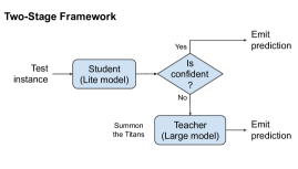
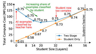
Figure 1: Left: A schematic of the proposed two-stage inference framework where after distillation we retain both the lightweight student model and the large teacher model. At inference time if the student finds an instance hard, we fall back to the teacher for a prediction. Right: The two-stage framework on CIFAR-100 image classification task using ResNets allows us to aggressively trade-off size of the student, thereby reducing the overall computation in expectation and achieving better accuracy compared to performing inference based on only the student. Note that the numbers annotated at each (student size, total compute cost) point on the plots denote the overall accuracy of the corresponding setup. For the two-stage inference, as we increase the size of the student, we can always achieve an accuracy of 0.75 by delegating an appropriate fraction of instances to the teacher. Compared to classifying all examples using the teacher, computation cost savings come from those instances where the student makes the final prediction.

In this paper, we focus on realizing the benefits of a large model on the hard instance without incurring the unnecessary large inference cost on prevalent easy instances. Towards this, we propose to employ a novel distillation-based two-stage inference framework in Figure 1 (left): First use a lightweight student model to make a prediction. If the student is confident, we emit the prediction and we want the student to be confident on all the easy instances, which should be a large fraction of the test time queries. When the student is in doubt, ideally only for a small number of hard examples, we fall-back to the large teacher. Our main contributions for leveraging the excellent performance of large models to realize a desirable inference cost vs. performance trade-off are as follows.

• The instance-aware two-stage inference mechanism crucially relies on the ability of the student model to detect the “hardness” of an input instance on the fly and routing it to the large model. To enable this routing, we propose modified distillation procedures. In particular, we employ novel distillation loss functions (cf. Sec. 4) such that the student gets penalized heavily for making mistakes on easy examples while for harder out-of-domain examples we encourage the student to be less confident, e.g., the prediction distribution be closer to the uniform distribution.

• We conduct a detailed empirical evaluation of the proposed distillation-based two-stage inference framework (cf. Sec. 5) and show that it allows us to much more aggressively trade-off size of the student for multiple image classification and natural language processing (NLP) benchmarks. Interestingly, as summarized in Figure 1, there is a sweet spot where we can achieve the same accuracy as the teacher with 45% less compute. This benefit is further magnified when considering only in-domain examples. Thus, we can reduce the overall computation over the data distribution and achieve better accuracy than performing inference with only the student model.

Note that, traditionally, the distillation approach aims to utilize a complex model to learn a simple model that has its overall performance as close to the complex model as possible. This is done under the assumption that during the inference time one can ‘throw away’ the complex model and rely on only the simple model for the final predictions. We would like to highlight that our goal is not to train a student/simple model that will be used as a standalone model to generate predictions.

It’s worth mentioning that the proposed two-stage inference can also be useful in a modern setup like edge computing and 5G cloudlets (Fang et al., 2019), where a lightweight student model runs on a device to make most of the predictions with low latency and only once in a while a hard instance is delegated to a shared large teacher model running in the cloud.

2 Related work

Techniques to reduce inference cost for deep models mainly fall under two different approaches: quantization and pruning, and adaptive computation.

Quantization and pruning. The primary way suggested in the literature to accelerate predictions from deep neural networks has been quantization and pruning (Mozer and Smolensky, 1988; LeCun et al., 1989; Hassibi and Stork, 1993; Li et al., 2020; Carreira-Perpinán, 2017; Howard et al., 2019). Significant progress was made by introducing Huffman encoding methods for non-uniform quantization which led to a reduction in network sizes by orders of magnitude and up to 4x reduction in overall prediction cost (Han et al., 2015). Since then pruning and quantization have been widely adopted in computer vision and more details can be found in the recent survey by Liang et al. (2021). In the NLP domain, Gordon et al. (2020); Zadeh et al. (2020) proposed pruning BERT during training, which resulted in 30%-40% reduction in model size with minimal effect on the accuracy of the final task, however, not much compute/time savings was observed as arbitrary sparsity might not be leveraged by modern hardware accelerators. Towards this, structured pruning is more beneficial, as it removes a series of weights that correspond to an entire component of the model  (Ganesh et al., 2020). In transformers, this would correspond to pruning out entire attention heads (Kovaleva et al., 2019; Raganato et al., 2020) or encoder units (Fan et al., 2019). Our proposed approach of two-stage inference is complementary to such techniques and can be combined with these to further reduce the inference cost.

Adaptive computation. In line with our proposed approach, there have been works trying to adapt the amount of computation of neural model based on an input instance. Effort in this space started in the vision community for enabling real-time object detection by Rowley et al. (1998) and later formalized by Viola and Jones (2001). The basic idea was to design a cascade of independent classifier and reject early on and cheaply. The idea has been generalized from a linear chain of cascaded classifiers to trees (Xu et al., 2014). Instead of combining many independent classifiers, a similar idea to stop early has emerged in monolithic deep models. One approach to this problem is represented by Adaptive Computation Time (ACT) (Graves, 2016; Chung et al., 2016). ACT is a mechanism for learning a scalar halting probability, called the “ponder time”, to dynamically modulate the number of computational steps needed for each input. An alternative approach is represented by Adaptive Early Exit Networks (Bolukbasi et al., 2017), which gives the network the ability to exit prematurely - i.e., not computing the whole hierarchy of layers - if no more computation is needed. A modern incarnation of this approach in NLP with transformers encoders appeared in Schwartz et al. (2020); Liu et al. (2020); Dabre et al. (2020). This idea has been extended to generative tasks as well, where a number of decoder layers per time step are adapted in Elbayad et al. (2020). As a further generalization, Bapna et al. (2020) introduced “control symbols” to determine which components are skipped in a transformer, i.e. not all previous components need to be executed. Similar ideas had already existed in the vision community, for example, Wang et al. (2017a, 2018) introduced a method for dynamically skipping convolutional layers. All of these approaches are specialized to a task and rely on designing the whole pipeline from scratch which can be expensive if we want to achieve state-of-the-art (SoTA) performance. In contrast, we want to design efficient inference techniques achieving SoTA performance by only training cheap components, like the student model using a novel distillation procedure, while leveraging existing SoTA large models without re-training or modifying them. Moreover, our approach is a generic framework to leverage the large models independent of the underlying model architecture and problem domain. Our proposed approach ensures that large model is only invoked on instances that necessarily benefit from its large model capacity and a lite distilled model suffices to predict a large portion of test instances.

3 Background

3.1 Multiclass classification

Consider a standard multiclass classification problem where given an instance $x\in\mathscr{X}$, the objective is to classify the instance as a member of one of the $L$ classes, indexed by $\mathscr{Y}\triangleq[L]$. In the most common setting, given a training set comprising of $n$ instance and label pairs or training examples $S_{n}=\{(x_{i},y_{i})\}_{i\in[n]}$, one learns a classification model $f:\mathscr{X}\to\mathbb{R}^{L}$, where $f(x)=(f(x)_{1},\ldots,f(x)_{L})$ represent the model scores assigned to instance $x$ for $L$ classes. Based on the model scores, an instance can be predicted to belong to class $\hat{y}_{x}\triangleq\arg\max_{i\in[L]}f(x)_{i}$. Accordingly, the model (top-$1$) accuracy is defined as

$$\mathbb{P}\left[\hat{y}_{x}=y\right]=\mathbb{E}_{X,Y}\left[\mathds{1}_{\hat{y}_{x}=y}\right]=1-\mathbb{E}_{X,Y}\left[\mathds{1}_{\hat{y}_{x}\neq y}\right].$$ (1)

Ideally, one prefers a classification model with a high accuracy. Let $\ell:\mathscr{Y}\times\mathbb{R}^{L}\to\mathbb{R}$ be a surrogate loss function such that $\ell(y,f(x))$ closely approximates the misclassification error $\mathds{1}_{\hat{y}_{x}\neq y}$. Typically, given the training set $S_{n}$ and the loss function $\ell$, one selects a desired classification model via empirical risk minimization (ERM). Softmax cross-entropy loss is one of the most widely used surrogate loss functions for multiclass classification: Given model scores $f(x)=(f(x)_{1},\ldots,f(x)_{L})$, one computes the softmax distribution

$$\hat{p}_{f,x}(i)={e^{\tau\cdot f(x)_{i}}}/{\sum\nolimits_{j\in[L]}e^{\tau\cdot f(x)_{j}}},~{}~{}\text{for}~{}~{}y\in[L],$$ (2)

where $\tau$ denotes the temperature parameter of the softmax operation. Further, we define $p_{y}\in\{0,1\}^{L}$ to be the one-hot label distribution corresponding to the true label $y\in[L]$, which has non-zero value at only $y$-th coordinate. Now, softmax cross-entropy loss corresponds to the distance between the distributions $p_{y}$ and $\hat{p}_{f,x}$, as measured by the cross-entropy function.

$$\ell(y,f(x))=H(p_{y},\hat{p}_{f,x})\triangleq-\sum\nolimits_{i\in[L]}p_{y}(i)\cdot\log\hat{p}_{f,x}(i).$$

3.2 Model distillation

Distillation is a celebrated training techniques that utilizes one model’s scores to train another model (Bucilǎ et al., 2006; Hinton et al., 2015). The former model is typically referred to as the ‘teacher’ model while the latter model is called the ‘student’ model. During distillation, given a teacher model $g:\mathcal{X}\to\mathbb{R}^{L}$ and an example $(x,y)\in\mathscr{X}\times\mathscr{Y}$, one first defines the teacher (softmax) distribution $\hat{p}_{g,x}(i)$ as per (2). Now, as opposed to utilizing the ‘one-hot’ label distribution $p_{y}$, we treat $\hat{p}_{g,x}(i)$ as the pseudo label distribution and define the distillation version of the softmax cross-entropy loss for the student model $f:\mathcal{X}\to\mathbb{R}^{L}$ as $\ell_{\rm distill}(g(x),f(x))=H(\hat{p}_{g,x},\hat{p}_{f,x})$. For $a,b\in\mathbb{R}_{+}$, distillation involves minimizing

$$\frac{a}{n}\sum\nolimits_{i\in[n]}\ell(y_{i},f(x_{i}))+\frac{b}{n}\sum\nolimits_{i\in[n]}\ell_{\rm distill}(g(x_{i}),f(x_{i}))$$ (3)

Note that the objective in (3) utilized both the true labels $\{y_{i}\}$ and the the teacher scores $\{g(x_{i})\}$. When $b=0$, this reduces to the standard training. More interestingly, when $a=0$, (3) correspond to training with solely $\hat{p}_{g,x}(i)$ – a fairly common way to utilize distillation (Menon et al., 2020a).

Remark 1.

For distillation, teacher models are usually much more complex and powerful as compared to student models (Bucilǎ et al., 2006; Hinton et al., 2015). However, the distillation with an equally complex, and even a simpler, teacher model has been shown to improve the quality of the student model via distillation (see, e.g., Rusu et al., 2016; Furlanello et al., 2018; Yuan et al., 2020).

4 Distillation for two-stage inference

We now propose various distillation approaches to power the proposed two-stage inference framework. Recall that we intend to obtain a lightweight student model that can generate highly accurate predictions on easy instances and route hard instances to the large teacher model. This raises an interesting question if one needs to modify the distillation process in any way whatsoever to aid our objective as typically distillation envisions the student model to be used as a standalone model.

Towards this, we explore a general distillation framework that partitions the training examples $S$ into two groups: 1) easy instances $S_{\rm easy}$ and 2) hard instances $S_{\rm hard}$. Accordingly, we modify the distillation process such that the student incurs larger loss when it makes incorrect predictions $S_{\rm easy}$. Furthermore, we penalize the student less for making mistakes on $S_{\rm hard}$, which we accomplish by carefully designed supervision during the distillation. Now, we present two specific realizations of the above generic distillation framework based on two different strategies to partition the training examples into $S_{\rm easy}$ and $S_{\rm hard}$.

4.1 Class-specific distillation

Many real-world data distributions exhibit a long-tail behavior where most of the instances we observe belong to a small number of classes, and the remaining classes are represented by very few instances. This has sparked a long line of work on improving model performance on the tail classes (see, e.g., Cui et al., 2019; Cao et al., 2019; Kang et al., 2020; Menon et al., 2021). In contrast, we explore an orthogonal direction and leverage the data imbalance to enable efficient inference with large models. In particular, for $\mathcal{L}_{\rm in}\subseteq[L]$, we define

$$S_{\rm easy}=\{(x,y)\in S:y\in\mathcal{L}_{in}\}\quad\text{and}\quad S_{\rm hard}=S\backslash S_{\rm easy}=\{(x,y)\in S:y\notin\mathcal{L}_{in}\}.$$

Thus, we require the lite model to perform well only on a subset of classes $\mathcal{L}_{\rm in}$ and route the examples from the remaining classes to the large model. Here, we hypothesize that the smaller model can better utilize its limited capacity to perform well on a subset of classes. Now, setting $\mathcal{L}_{\rm in}$ to be the head classes will ensure that the lite model itself tries to predict the examples from the head classes. Since the underlying data-distribution is long-tail, only the examples from the tail classes (and a few hard examples from the head classes depending on the exact implementation details described later) are sent to the large model during inference.

With this general approach in mind, we propose a class-specific distillation approach. Now, given a large teacher model $g$ and example $(x,y)$, we define a pseudo label distribution $\widetilde{p}^{\rm class}_{g,x}$ as follows:

$$\widetilde{p}^{\rm class}_{g,x}=\begin{cases}\hat{p}_{g,x}&\text{if}~{}y\in\mathcal{L}_{\rm in},\\ (1-\alpha)\cdot p_{y}+\frac{\alpha}{L}\cdot\mathbf{1}&\text{if}~{}y\in[L]\backslash\mathcal{L}_{\rm in},\end{cases}$$ (4)

where $\hat{p}_{g,x}$ and $p_{y}$ denote the teacher’s softmax distribution and the one-hot label distribution, respectively. In addition, $\alpha\in[0,1]$ denotes a label-smoothing parameter. Now, we train a lite student $f:\mathcal{X}\to\mathbb{R}^{L}$ with the distillation loss

$$\ell_{\rm distill}^{\rm class}\big{(}g(x),f(x)\big{)}\triangleq H\big{(}\widetilde{p}^{\rm class}_{g,x},\hat{p}_{f,x}\big{)}.$$ (5)

Note that the loss in (5) utilizes teacher softmax distribution for classes in $\mathcal{L}_{\rm in}$ and relies on label-smoothed one-hot distribution for the remaining classes. This loss has two desirable properties for our two-stage inference objective: 1) As a result of standard distillation, the lite student behaves as a well-calibrated model with good performance on the examples from the classes in $\mathcal{L}_{\rm in}$. 2) Due to standard label-smoothing (Szegedy et al., 2016; Müller et al., 2019), the lite student achieves a smaller margin on the examples belonging to the classes in $[L]\backslash\mathcal{L}_{\rm in}$.

Let $f_{\mathcal{L}_{\rm in}}$ be the lite student model obtained by minimizing the loss in (5). Now, given a test instance $x\in\mathcal{X}$, we first run inference with the lite model to obtain $f_{\mathcal{L}_{\rm in}}(x)$. Subsequently, we decide if we need to make the final prediction based on $f_{\mathcal{L}_{\rm in}}(x)$ or delegate the example to the large teacher $g$ to obtain the final prediction. We identify two useful delegation schemes, which we detail next.

Class-based delegation. Recall that the class-specific distillation aims to utilize the lite model to classify only the examples belonging to the classes in $\mathcal{L}_{in}$. Thus, the prediction made by $f_{\mathcal{L}_{\rm in}}$ serves as a natural candidate for the delegation. In particular, when

$$\hat{y}_{\rm student}(x)\triangleq\arg\max\nolimits_{j\in[L]}f_{\mathcal{L}_{\rm in}}(x)\in\mathcal{L}_{\rm in},$$

we declare $\hat{y}_{\rm student}(x)$ as the final prediction. Otherwise, $x$ is sent to the teacher and $\hat{y}_{\rm teacher}(x)\triangleq\arg\max_{j\in[L]}g(x)$ becomes the final prediction.

Margin-based delegation. The class-based delegation is designed under the assumption that the lite model achieves high accuracy on the examples belonging to the classes in $\mathcal{L}_{\rm in}$ and identifies the examples from $[L]\backslash\mathcal{L}_{\rm in}$ with high fidelity. Both of these assumptions don’t always hold in practice. In particular, $f_{\rm\mathcal{L}_{\rm in}}$ may find some instances from $\mathcal{L}_{\rm in}$ hard and incorrectly predict a wrong class in $\mathcal{L}_{\rm in}$ when presented with those instances. Similarly, $f_{\rm\mathcal{L}_{\rm in}}$ may predict a class from $\mathcal{L}_{\rm in}$ when the test instance belongs to $[L]\backslash\mathcal{L}_{\rm in}$.

Recall that the distillation loss in (5) is designed to ensure that $f_{\rm\mathcal{L}_{\rm in}}$ is well-calibrated on the instances from $\mathcal{L}_{\rm in}$; as a result, it attains small margin on hard instances from $\mathcal{L}_{\rm in}$. Moreover, by design, $f_{\rm\mathcal{L}_{\rm in}}$ realizes small margin on the instances from $[L]\backslash\mathcal{L}_{\rm in}$. Thus, one can utilize the margin of the lite model $f_{\mathcal{L}_{\rm in}}$ to perform delegation. Towards this, recall that

$$\gamma_{\rm f_{\rm\mathcal{L}_{\rm in}}}(x)\triangleq\hat{p}_{f_{\rm\mathcal{L}_{\rm in}},x}([1])-\hat{p}_{f_{\rm\mathcal{L}_{\rm in}},x}([2])$$ (6)

denotes the margin realized by $f_{\rm\mathcal{L}_{\rm in}}$ on $x$. Here, $\hat{p}_{f_{\rm\mathcal{L}_{\rm in}},x}([i])$ denotes the $i$-th largest element of the vector $\hat{p}_{f_{\rm\mathcal{L}_{\rm in}},x}$. Now, given a design parameter $\rho\in(0,1)$, we assign the following final prediction to a test instance $x\in\mathcal{X}$.

$$\hat{y}(x)=\begin{cases}\hat{y}_{\rm student}(x)&\text{if}~{}\gamma_{\rm f_{\rm\mathcal{L}_{\rm in}}}(x)\geq\rho,\\ \hat{y}_{\rm teacher}(x)&\text{if}~{}\gamma_{\rm f_{\rm\mathcal{L}_{\rm in}}}(x)<\rho.\end{cases}$$ (7)

The margin-based delegation aims to ensure that hard instances from $\mathcal{L}_{\rm in}$ as well as all instances in $[L]\backslash\mathcal{L}_{\rm in}$ get routed to the teacher for the final prediction.

Remark 2.

The distillation based on the loss in (5) constitutes only one of many possible ways to transfer the performance of a teacher over a subset of classes to a lite student. We discuss two other class-specific distillation-based approaches in Sec. A of the appendix and evaluate those in Sec. 5.

4.2 Margin-based distillation

As discussed before, the margin assigned to an instance by a model is a natural proxy for the hardness of the instance, as viewed by the model. In Sec. 4.1, we utilize the margins assigned by the student to delegate the examples to the teacher. This raises an interesting question if one can utilize the margins to partition the training data into $S_{\rm easy}$ and $S_{\rm hard}$ example during the distillation. Towards this, given a teacher $g$ and a parameter $\rho_{\rm tr}\in(0,1)$, we add a training example $(x,y)$ to $S_{\rm easy}$ iff

$$\gamma_{g}(x)\triangleq\hat{p}_{g,x}([1])-\hat{p}_{g,x}([2])>\rho_{\rm tr}.$$ (8)

Given this data partition, for an example $(x,y)$, we define the pseudo label distribution as follow:

$$\widetilde{p}^{\rm margin,L}_{g,x}=\begin{cases}(\hat{p}_{g,x}(1),\ldots,\hat{p}_{g,x}(L))&\mbox{if }(x,y)\in S_{\rm easy}\\ {(1-\alpha)\cdot p_{y}+\frac{\alpha}{L}\cdot\mathbf{1}}&\mbox{otherwise }.\end{cases}$$ (9)

Now, we obtain a (lite) student $f^{L}_{\rho_{\rm tr}}:\mathcal{X}\to\mathbb{R}^{L}$ by minimizing

$$\ell^{\rm margin,L}_{\rm distill}\big{(}g(x),f(x)\big{)}=H(\widetilde{p}^{\rm margin,L}_{g,x},\hat{p}_{f,x}).$$ (10)

For the two-stage inference, given a test instance $x$, we make the following final prediction.

$$\hat{y}(x)=\begin{cases}\hat{y}_{f^{L}_{\rho_{\rm tr}}}=\arg\max_{j}{f^{L}_{\rho_{\rm tr}}}(x)_{j}&\text{if}~{}\gamma_{f^{L}_{\rho_{\rm tr}}}(x)\geq\rho,\\ \hat{y}_{\rm teacher}(x)&\text{otherwise},\end{cases}$$

where $\hat{y}_{f^{L}_{\rho_{\rm tr}}}=\arg\max_{j}{f^{L}_{\rho_{\rm tr}}}(x)_{j}.$

Remark 3.

For a small value of $\rho_{\rm tr}$, we expect the student to make the correct prediction on almost all examples. Thus, the margin-based distillation proposed above becomes very similar to the normal distillation discussed in Sec. 3.2. On the other hand, for large values of $\rho_{\rm tr}$, the student is expected to do well on only a small subset of examples during training and be able to identify the rest of the examples as hard instances that need to be routed to the teacher.

Similar to class-specific distillation, there are multiple potential variants of the margin-based distillation. We discuss one such variant that relies on an ‘abstain’ class in Sec. C of the appendix.

5 Experiments

We now conduct a comprehensive empirical study of our distillation-based two-stage inference procedure. In particular, we evaluate various distillation frameworks introduced in Sec. 4 along with different choices of delegation methods. On standard image classification tasks, we establish. that:

• A large improvement in accuracy over the student-only approach can be realized by delegating only a small fraction of examples to the large teacher model (Sec. 5.1). This validates our claim that one can rely on a much smaller student and achieve an accuracy similar to the teacher-only approach with a small increment in inference cost.

• Advantages of the two-stage inference are even more pronounced if we focus on the in-domain performance, where the in-domain portion of the instance space corresponds to a subset of classes or instances with a large margin (based on the large teacher model). This validates the utility of two-stage inference for those real-world settings where a large data imbalance exists in favor of in-domain instances (Sec. 5.2).

• Class-specific distillation defined by (5) indeed achieves the desired behavior where the student enables a clear dichotomy among the in-domain and out-of-domain instances. By varying the label-smoothing parameter, we can improve in-domain model performance and delegate a small number of instances to the teacher at the cost of performance on the entire test data (Sec. 5.2).

Furthermore, by delegating a small fraction of hard instances to a large teacher model, our proposed class-specific distillation and a variant of margin-based distillation enable efficient inference on sentence classification and reading comprehension tasks in the NLP domain, respectively (Sec. 5.3).

We mainly focus on three benchmark image datasets – CIFAR-100 (Krizhevsky, 2009), ImageNet-1k (Russakovsky et al., 2015), and ImageNet-21k (Deng et al., 2009). In addition, we also evaluate the proposed two-stage inference procedure on a sentence classification task based on MNLI (Williams et al., 2018) and a reading comprehension task based on SQuAD dataset (Rajpurkar et al., 2016). On image classification tasks, we use EfficientNet-L2 (Xie et al., 2020) as the large teacher. As for the lite student, we utilize ResNet (He et al., 2016a, b) and MobileNetV3 (Howard et al., 2019) for CIFAR-100 and ImageNet, respectively. For the sentence classification and reading comprehension tasks, RoBERTa-Large (Liu et al., 2019) and T5-11B (Raffel et al., 2019) serve as the teachers, respectively. We use MobileBERT (Sun et al., 2020) as the lite student for both MNLI and SQuAD. We provide a detailed description in Sec. D of the appendix.

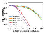
(a) Overall accuracy

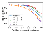
(b) In-domain accuracy

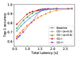
(c) Latency vs. in-domain accuracy

Figure 2: Comparison of various class-specific distillation methods on CIFAR-100. Baseline denotes the standard distillation from (3). ${\rm CD}$-I, ${\rm CD}$-II, and ${\rm CD}$-III denote the class-specific distillation approaches defined in Sec. 4.1, Sec. A.1, and Sec. A.2, respectively, with $|\mathcal{L}_{\rm in}|=L^{\prime}=30$. Accordingly, we compute in-domain accuracy on test instances from the $30$ classes in $\mathcal{L}_{\rm in}$. Here, each lite student (ResNet-32) employs margin-based delegation to the teacher. The right-most plot depicts the (inference) latency vs. in-domain accuracy trade-off for the two-stage inference procedure.

5.1 Overall accuracy gains

We begin by establishing the utility of the two-stage inference procedure for overall performance improvement. Towards this, Fig. 2, 3, and 5 (in appendix) depict the two-stage overall accuracy achieved by various class-specific distillation approaches via margin-based delegation. Besides, we also include conventional model distillation as Baseline in our evaluation. Note that, for all approaches, allowing the lite student model to delegate hard instances (the ones with a small margin) to the large teacher significantly increases the accuracy as compared to the performance of (one-stage) student-only inference approach. Focusing on CIFAR-100, both Baseline and CD-I can approximate the performance of the teacher model by delegating only $\sim$40% test instance, which translates to $\sim$60% reduction in the inference cost as compare to the large teacher (cf. Fig. 2). Here, we note that CD-II and CD-III train the student to make the correct prediction on only the instances belonging to the classes in $\mathcal{L}_{\rm in}$, leading to poor overall accuracy on the entire test set. However, unsurprisingly, as student delegates more instances to the teacher, the two-stage overall accuracy improves. Similar conclusions also hold on ImageNet datasets (cf. Fig. 3 and 5). Table 1 and 4 (in the appendix) show that the class-specific distillation based two-stage inference leads to similar improvements in the overall accuracy when we employ class-based delegation from Sec. 4.1.

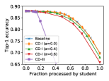
(a) Overall accuracy

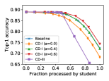
(b) In-domain accuracy

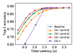
(c) Latency vs. in-domain accuracy

Figure 3: Comparison of various class-specific distillation methods on ImageNet-1k. Baseline denotes the standard distillation from (3). ${\rm CD}$-I and ${\rm CD}$-III denote the class-specific distillation approaches defined in Sec. 4.1 and Sec. A.2, respectively, with $|\mathcal{L}_{\rm in}|=L^{\prime}=300$. Accordingly, we compute in-domain accuracy on the test instances from the $300$ classes in $\mathcal{L}_{\rm in}$. Here, each lite student (MobileNetV3-0.75) employs margin-based delegation. The right-most plot depicts the (inference) latency vs. in-domain accuracy trade-off for the two-stage inference procedure.

	Approach	In-domain			Overall
		Accuracy	Fraction		Accuracy	Fraction
ResNet-32	Baseline	0.71	1.00		0.72	1.00
	CD-I ($\alpha=0.0$)	0.88	0.74		0.88	0.26
	CD-I ($\alpha=0.6$)	0.88	0.84		0.86	0.32
	CD-II	0.78	1.00		0.24	1.00
	CD-III	0.91	0.69		0.90	0.25
ResNet-56	Baseline	0.75	1.00		0.75	1.00
	CD-I ($\alpha=0.0$)	0.89	0.77		0.90	0.27
	CD-I ($\alpha=0.6$)	0.90	0.82		0.88	0.29
	CD-II	0.80	1.00		0.24	1.00
	CD-III	0.92	0.71		0.90	0.25

Table 1: Performance of two-stage inference procedure on CIFAR-100. The student employs class-specific distillation with $|\mathcal{L}_{\rm in}|=L^{\prime}=30$, with in-domain referring to the instances from the classes in $\mathcal{L}_{\rm in}$. During inference we, use an appropriate class-based delegation method. See Fig. 2 for the identity of the distillation approaches. Fraction denotes the fraction of test instances where the student model makes the final prediction. Unlike margin-based delegation, for given teacher and student models, we obtain a single value of (Accuracy, Fraction) tuple with class-based delegation.

5.2 In-domain performance

Next, we verify that two-stage distillation is even more beneficial in those real-world settings where ML models encounter heavily imbalanced data during the inference. Ideally, the lite student model should make a prediction on frequent but easy instances and delegate rare but hard instances to the large teacher. This would ensure that the two-stage inference procedure realizes high overall accuracy (compared to inference with only the student) while significantly lowering the inference cost (compared to inference with only the teacher). With this in mind, we evaluate the performance of the two-stage inference procedure on in-domain (so-called easy instances). By design, for class-specific distillation, in-domain instances belong to the classes in $\mathcal{L}_{\rm in}$. Similarly, for the margin-based distillation, in-domain instances are the ones where teacher assigns a large margin $\rho$.

For CIFAR-100, Fig. 2 shows that two-stage inference achieves much better in-domain (defined by $|\mathcal{L}_{\rm in}|=30$ classes) accuracy as compared to overall accuracy. This implies that in a real-world setting where in-domain instances are frequent, the two-stage inference can efficiently achieve very good overall performance by having the student predict most of the in-domain instances. Note that overall performances in such a scenario (with data-imbalance) is not captured by Fig. 2 which is based on fair balanced test data. Instead of aiming to imitate the data imbalance encountered in practice, we have separately highlighted the performance of two-stage inference on the in-domain instances. This shows that the more imbalanced the data is the more advantageous two-stage distillation would be in terms of saving the inference cost without affecting the classification performance. As per Fig 2, we essentially maintain same accuracy as the teacher but reduce latency by more than 2x. Here, we also note that Fig. 2 implies that two-stage inference would indeed enable one to approximate the teacher performance on all instances, whether they belong to in-domain or not.

Interestingly, Fig. 2 indicates that CD-I with margin-based delegation gives a favorable tradeoff between in-domain and (balanced) overall accuracy. The label-smoothing parameter $\alpha$ in (4) helps create a dichotomy between in-domain and out-of-domain instances. The larger values of $\alpha$ ensure that the student assigns a smaller margin to out-of-domain examples and tries to improve its performance on in-domain instances. This is reflected in Fig. 2 where CD-I with large $\alpha$ achieves higher accuracy by predicting a larger fraction of in-domain instances at the student. We note the similar trend in Table 1 where we combine class-specific distillation with class-based delegation

We also evaluate the in-domain two-stage performance of class-based distillation on ImageNet-1k with $|\mathcal{L}_{\rm in}|=300$. The conclusions from Fig. 3, 3 and Table 4 (in the appendix) are similar to those observed on CIFAR-100. Also, see Fig. 5 (in the appendix) for the identical trends on ImageNet-21k. Finally, we also studied the in-domain performance of two-stage inference enabled by margin-based distillation from Sec. 4.2 on both CIFAR-100 and ImageNet-1k in the appendix.

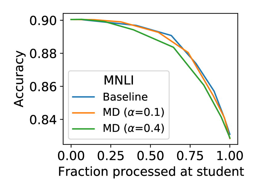
(a) Overall accuracy

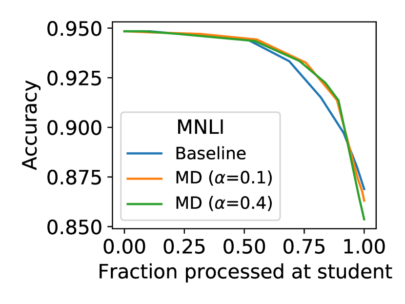
(b) In-domain accuracy

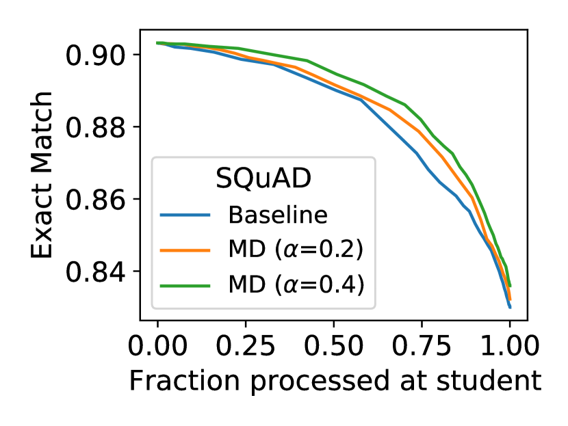
(c) Overall accuracy

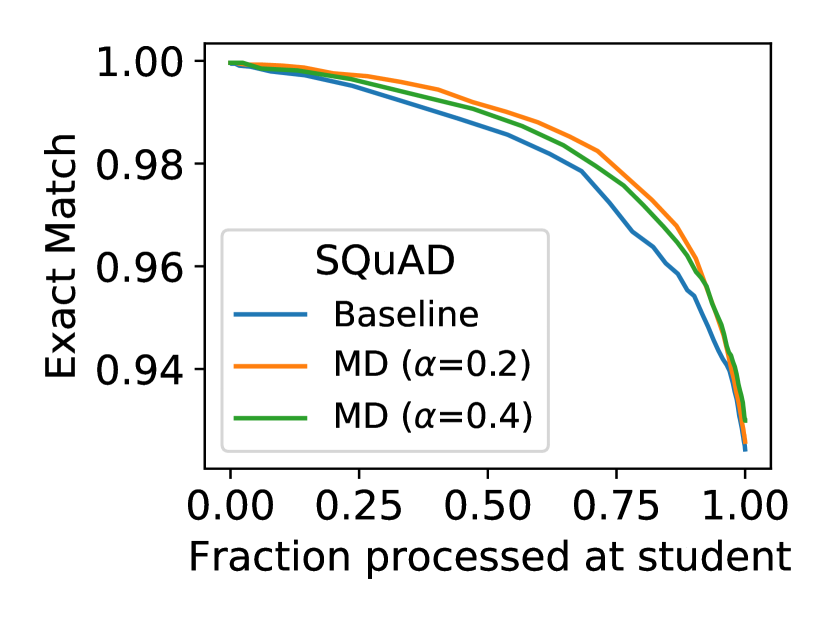
(d) In-domain accuracy

Figure 4: Performance of the proposed two-stage inference on NLP tasks. Left half: Overall and in-domain accuracy of the margin-based distillation coupled with margin-based delegation on MNLI. Here baseline corresponds to the two-stage inference enabled by the standard distillation (cf. (3)). Right half: Overall and in-domain accuracy (exact match) comparison of margin-based distillation on SQuAD task. Here, Baseline denotes a normally trained student used in combination with the teacher. Note that MD denotes a margin-based distillation with label smoothing.

5.3 Two-stage inference in NLP domain

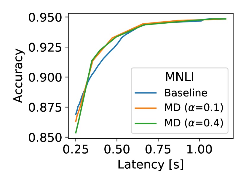
(a) Latency vs. in-domain accuracy (MNLI)

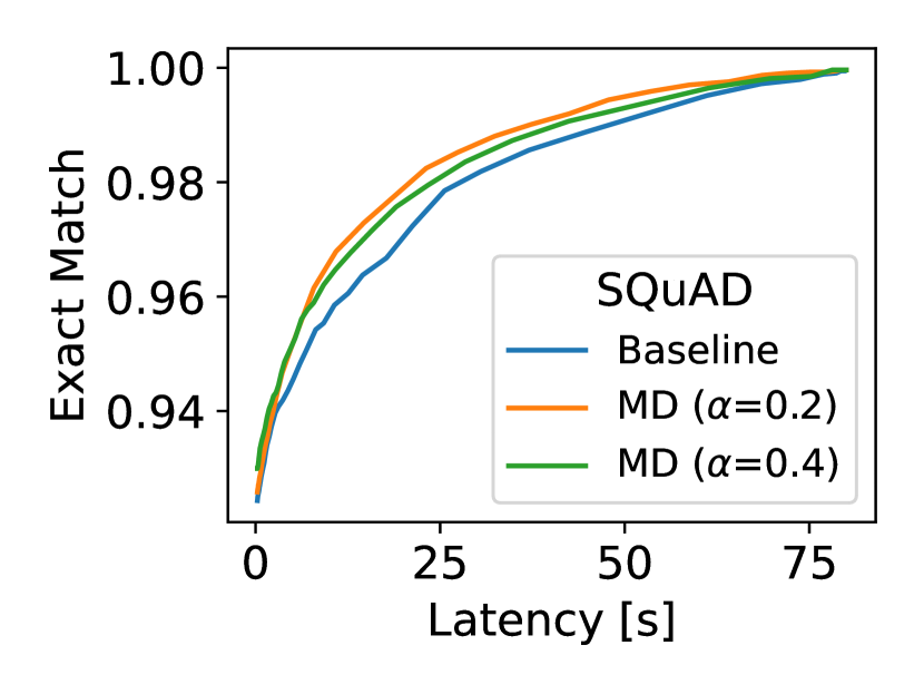
(b) Latency vs. in-domain accuracy (SQuAD)

Figure 8: The inference-latency vs. in-domain performance trade-off realized by the two-stage inference procedure on the NLP tasks. MD denotes the margin-based distillation with label smoothing parameter $\alpha$. Left: On MNLI dataset, RoBERTa-Large and MobileBERT are used as the teacher and student models, respectively. Here, Baseline corresponds to the two-stage inference enabled by the standard distillation (cf. (3)). Right: On SQuAD dataset, T5 and MobileBERT are used as the teacher and student models, respectively. Here, Baseline denotes a normally trained MobileBERT used in combination with T5 model.

Sentence classification task. Fig. 4 and 4 show the performance of our proposed two-stage inference framework on MNLI. Since it has only 3 classes, we employ margin-based distillation (with $\rho_{\rm tr}=8.0)$ from (9) with margin-based delegation. Our conclusion for the image classification also extends to the text domain and the two-stage inference framework enables a lite student to leverage high-quality teacher by delegating a small portion of (hard) instances to the teacher. We provide inference-latency vs. in-domain performance trade-off for MNLI in the appendix (cf. Fig. 8).

Reading comprehension task. To showcase the generality of our approach, we apply the two-stage inference method to a machine comprehension task (SQuAD), where there is a fundamental mismatch between student architecture which is based on span selection whereas teacher is based on a richer but more expensive encoder-decoder architecture. Thus, one cannot do standard distillation by transferring logits from teacher to students, but a suitable modification of margin-based distillation from (9) still works. We partition the training examples into easy and hard instances by thresholding teacher’s log-likelihood of ground-truth answer given the context. While training student, for easier examples, we use one hot labels for the start and end span as no teacher logits are available. Whereas for hard examples, we still employ label smoothing. We try two values $\alpha=0.2,0.4$ in the experiments. Our results in Fig. 4 and 4, which has similar conclusions to the classification experiments. See Fig. 8 for the inference-latency vs. in-domain performance trade-off achieved by the two-stage inference.

6 Discussion

We propose a distillation-based two-stage inference framework to efficiently leverage large models with prohibitively large inference costs in real-world settings. Given a large model, we distill a lite student that utilizes its limited model capacity to perform well on easy (in-domain) instances and can identify hard (out-of-domain) instances. When deployed in tandem, the lite model generates the final prediction on easy but frequent instances and delegates hard but rare instances to the large model. This ensures much higher performance (compared to inference based on only the lite model) and a much smaller inference cost (compared to inference with only the large model). We propose various distillation methods to enable such two-stage inference. We establish the utility of these approaches for realizing efficient and accurate inference on both image classification and NLP benchmarks. The advantages of our proposed approaches become even more pronounced as the imbalance between in-domain and out-of-domain data increases during inference.

Generalizing our framework to design a multi-stage inference procedure is a natural direction for future research. To enhance the applicability of our method to wider settings, another research direction would be to devise a principled approach for applying our method to other architectures including non-parametric models like k-NN, generalizing what we did for reading comprehension.

Appendix A Variants of class-specific distillation

Here, we present two additional variants of class-specific distillation that enable transferring the performance of a large teacher model to a lite student model on a subset of class. Subsequently, the lite student can be employed in our two-stage inference framework.

A.1 In-domain class-distillation

Since we do not intend the student to make the final prediction on an instance from $[L]\backslash\mathcal{L}_{\rm in}$, we can train the student to perform an $|\mathcal{L}_{\rm in}|=|L^{\prime}|$-way classification. In particular, given a teacher $g$ and example $(x,y)$, we define a pseudo-label distribution:

$$\widetilde{p}^{{\rm class},L^{\prime}}_{g,x}=\begin{cases}\hat{p}^{L^{\prime}}_{g,x}\in[0,1]^{L^{\prime}}&\text{if}~{}y\in\mathcal{L}_{\rm in},\\ \frac{1}{L^{\prime}}\cdot\mathbf{1}\in\mathbb{R}^{L^{\prime}}&\text{if}~{}y\in[L]\backslash\mathcal{L}_{\rm in}.\end{cases}$$ (11)

Here, $\hat{p}^{L^{\prime}}_{g,x}$ denotes the softmax distribution restricted to $\mathcal{L}_{\rm in}$:

$$\hat{p}^{L^{\prime}}_{g,x}(j)={e^{g(x)_{j}}}/{\sum\nolimits_{i\in\mathcal{L}_{\rm in}}e^{g(x)_{i}}}~{}~{}\text{for}~{}j\in\mathcal{L}_{\rm in}.$$ (12)

Now we get the student $f_{\mathcal{L}_{\rm in},L^{\prime}}:\mathcal{X}\to\mathbb{R}^{L^{\prime}}$ by minimizing

$$\ell^{\rm class,L^{\prime}}_{\rm distill}\big{(}g(x),f(x)\big{)}=H\big{(}\widetilde{p}^{{\rm class},L^{\prime}}_{g,x},\hat{p}_{f,x}\big{)}$$ (13)

A lite model $f_{\mathcal{L}_{\rm in},L^{\prime}}$ trained with the loss in (13) aims to classify an instance from $\mathcal{L}_{\rm in}$ to the correct class. At the same time, such a model is also trained to generate a non-informative uniform distribution $\frac{1}{L^{\prime}}\cdot\mathbf{1}$ on the instances from $[L]\backslash\mathcal{L}_{\rm in}$, which by definition corresponds to zero margin.

Now, given the student $f_{\mathcal{L}_{\rm in},L^{\prime}}$ and teacher $g$, one can define a two-stage inference by using margin-based delegation. In particular, for a test instance $x\in\mathcal{X}$, the final prediction becomes

$$\hat{y}(x)=\begin{cases}\arg\max_{j\in[L^{\prime}]}f_{\mathcal{L}_{\rm in},L^{\prime}}(x)_{j}&\text{if}~{}\gamma_{f_{\mathcal{L}_{\rm in},L^{\prime}}}(x)\geq\rho,\\ \arg\max_{j\in[L]}g(x)_{j}&\text{if}~{}\gamma_{f_{\mathcal{L}_{\rm in},L^{\prime}}}(x)<\rho,\end{cases}$$

where $\gamma_{f_{\mathcal{L}_{\rm in},L^{\prime}}}(x)$ is the margin assigned to $x$ by the student $f_{\mathcal{L}_{\rm in},L^{\prime}}$.

A.2 In-domain class-distillation with ‘abstain’ option.

We next explore another natural candidate for class-specific distillation, where the lite student aims to correctly classify an instance $x$ from $\mathcal{L}_{\rm in}$ and declares to ‘abstain’ on the instances from $[L]\backslash\mathcal{L}_{\rm i}$. To realize this, we train the student to perform an $(L^{\prime}+1)$-way classification: Given a teacher $g$ and example $(x,y)$, we define a pseudo label distribution:

$$\widetilde{p}^{{\rm class},L^{\prime}+1}_{g,x}=\begin{cases}(\hat{p}^{L^{\prime}}_{g,x},0)\in[0,1]^{L^{\prime}+1}&\text{if}~{}y\in\mathcal{L}_{\rm in},\\ (0,\ldots,0,1)&\text{if}~{}y\in[L]\backslash\mathcal{L}_{\rm in},\end{cases}$$

where $\hat{p}^{L^{\prime}}_{g,x}$ denotes the softmax distribution restricted to $L^{\prime}$ classes, as defined in (12). Now, one can perform the distillation by utilizing $\widetilde{p}^{{\rm class},L^{\prime}+1}_{g,x}$, i.e., minimize

$$\ell^{{\rm class},L^{\prime}+1}_{\rm distill}\big{(}g(x),f(x)\big{)}=H\big{(}\widetilde{p}^{{\rm class},L^{\prime}+1}_{g,x},\hat{p}_{f,x}\big{)}.$$ (14)

Note that (14) encourages the trained lite model $f_{\mathcal{L}_{\rm in},L^{\prime}+1}$ to predict $(L^{\prime}+1)$-th class, i.e., ‘abstain’ class, for all instances from $[L]\backslash\mathcal{L}_{\rm in}$. This leads to a natural abstain class-based delegation approach for two-stage inference. Let

$$\hat{y}^{\rm abstain}_{\rm student}(x)=\arg\max_{j\in[L^{\prime}+1]}f_{\mathcal{L}_{\rm in},L^{\prime}+1}(x)_{j}.$$

Then, given $f_{\mathcal{L}_{\rm in},L^{\prime}+1}$ and $g$, one makes the following final prediction for a test instance.

$$\hat{y}(x)=\begin{cases}\hat{y}^{\rm abstain}_{\rm student}(x)&\text{if}~{}\hat{y}^{\rm abstain}_{\rm student}(x)\leq L^{\prime},\\ \hat{y}_{\rm teacher}(x)&\text{if}~{}\hat{y}^{\rm abstain}_{\rm student}(x)=L^{\prime}+1.\end{cases}$$

In addition, analogous to (7), one can also define a two-stage inference procedure via margin-based delegation.

Remark 4.

Note that using an ‘abstain’ class is closely related to classification with a reject option (see Sec. B). However, as opposed to the traditional classification with the reject paradigm, we intend to provide supervision for the so call reject class as well.

Appendix B Classification with a reject option

There is a large literature on selective classification, also known as classification with a reject option or abstention Grandvalet et al. [2009], Bartlett and Wegkamp [2008], Cortes et al. [2016], Geifman and El-Yaniv [2017], Ramaswamy et al. [2018], Ni et al. [2019]. Here, one seeks a predictor $f\colon\mathcal{X}\to\mathcal{Y}\,\cup\{\perp\}$, where a prediction of $\perp$ denotes the classifier is uncertain. To avoid the degenerate solution of abstaining on all samples, one assumes a fixed rejection cost $c\in(0,1]$. The goal is to then trade-off the misclassification error on non-abstained samples with the total cost incurred on abstained samples, i.e., minimize the loss

$$\ell(y,f(x))=\mathds{1}_{y\neq f(x)\land f(x)\neq\perp}+c\cdot\mathds{1}_{f(x)=\perp}.$$ (15)

The Bayes-optimal classifier for this objective abstains on samples with high uncertainty on the “true” label, i.e., Ramaswamy et al. [2018]

$$f^{*}(x)=\begin{cases}\perp&\text{ if }\underset{y\in\mathcal{Y}}{\max}\,\mathbb{P}(y\mid x)\leq 1-c\\ \underset{y\in\mathcal{Y}}{\operatorname{argmax}}\,\mathbb{P}(y\mid x)&\text{ else. }\end{cases}$$ (16)

Appendix C Variant of margin-based distillation: using abstain class

Another natural approach for margin-based distillation is to utilize an ‘abstain’ class to encourage student to not spend its model capacity on correctly classifying hard instances (where teacher achieves a low-margin). Towards this, we can define the following pseudo label distribution for an example $(x,y)$.

$$\widetilde{p}^{\rm margin}_{g,x}=\begin{cases}(\hat{p}_{g,x}(1),\ldots,\hat{p}_{g,x}(L),0)&\mbox{if }(x,y)\in S_{\rm easy}\\ (0,\ldots,0,1)\in\{0,1\}^{L+1}&\mbox{otherwise }.\end{cases}$$

Now, we distill a lite student model $f^{L+1}_{\rho_{\rm tr}}:\mathcal{X}\to\mathbb{R}^{L+1}$ based on $\widetilde{p}^{\rm margin}_{g,x}$, i.e., we minimize

$$\ell^{\rm margin}_{\rm distill}\big{(}g(x),f(x)\big{)}=H(\widetilde{p}^{\rm margin}_{g,x},\hat{p}_{f,x})$$ (17)

Note that we train the student to perform an $(L+1)$-way classification, where it aims to classify an example in $S_{\rm easy}$ to one of $L$ original classes and the examples in $S_{\rm hard}$ to the ‘abstain’ class. Now, one may employ $g$ and $f^{L+1}_{\rho_{\rm tr}}$ to enable a two-stage inference procedure that makes the final prediction for a test instance $x\in\mathcal{X}$ as

$$\hat{y}(x)=\begin{cases}\hat{y}_{f^{L+1}_{\rho_{\rm tr}}}\qquad\text{if}~{}\hat{y}_{f^{L+1}_{\rho_{\rm tr}}}\leq L^{\prime}~{}\&~{}\gamma_{f^{L+1}_{\rho_{\rm tr}}}(x)\geq\rho,\\ \hat{y}_{\rm teacher}(x)~{}~{}~{}~{}~{}\text{otherwise},\end{cases}$$

where $\hat{y}_{f^{L+1}_{\rho_{\rm tr}}}=\arg\max_{j}{f^{L+1}_{\rho_{\rm tr}}}(x)_{j}$.

Appendix D Details of experimental setup

Datasets.

We use three benchmark image datasets – CIFAR-100 [Krizhevsky, 2009], ImageNet ILSVRC 2012 (a.k.a. ImageNet-1k) [Russakovsky et al., 2015], and ImageNet-21k [Deng et al., 2009]. CIFAR-100 contains 60k (50k train/10k test) images annotated with one of 100 object categories distributed uniformly. ImageNet (ILSVRC 2012), on the other hand, is a much larger dataset with 1.33M (1.28M train/50k test) images annotated with one of 1000 object categories also distributed uniformly. As for ImagenNet-21k, it originally contains images 12.8M from 21,843 classes. We select 17,203 classes with at least 100 images and create a balanced test set with 50 images from each of the selected classes. This remaining images from the selected classes provides us with a training set containing $\sim$11.8M images.

In addition to image datasets, we also evaluate the proposed distillation-based two-stage inference procedure on MNLI [Williams et al., 2018] and SQuAD datasets [Rajpurkar et al., 2016], which are standard sentence classification and QA benchmarks, respectively. MNLI dataset corresponds to a $3$-way classification task with 392,702 training examples and a matched test set consisting of 9,815 instances. As for the SQuAD dataset, it is a span selection task over a sequence length of 384 with 87,599 and 10,570 train and test examples, respectively.

Large teacher models.

For the image classification tasks, we use EfficientNet-L2 [Xie et al., 2020, Tan and Le, 2019, Foret et al., 2021] which is the state-of-art for image classification on multiple datasets. It is an optimized convolutional neural network pretrained on both ImageNet and unlabeled JFT-300M [Sun et al., 2017] with input resolution of 475. EfficientNet-L2 is a large model with 480M parameters which requires 478G FLOPs per inference and achieves an accuracy of 88.6% on ImageNet. For CIFAR-100, we used base EfficientNet-L2 model with a new fine-tuned classification layer achieving an accuracy of 94.4%. For the sentence classification task, a RoBERTa-Large [Liu et al., 2019] model serves as a teacher, which is pre-trained on a general purpose text corpus of 160 GB size. It is a transformer-based encoder model with 355M parameters that requires 155G FLOPs per inference while achieving an accuracy of 90.2% on MNLI. For the QA task requiring reading comprehension, we use T5-11B [Raffel et al., 2019] which exhibits competitive performance on a wide variety of NLP tasks. It is a text-to-text transformer architecture pretrained on a subset of the common crawl with sequence lengths of 512. T5-11B is a large model with 11B parameters and requires 6.6T FLOPs per inference achieving an accuracy of 90.2% on SQuAD.

Model	Parameters	FLOPs
ResNet-8	0.09 M	16 M
ResNet-14	0.19 M	30 M
ResNet-20	0.27 M	44 M
ResNet-32	0.46 M	72 M
ResNet-44	0.66 M	100 M
ResNet-56	0.85 M	128 M

Table 2: (Lite) ResNet models for CIFAR-100.

Model	Parameters	FLOPs
MobileNetv3-0.35	2.14 M	40 M
MobileNetv3-0.50	2.70 M	70 M
MobileNetv3-0.75	4.01 M	156 M
MobileNetv3-1.00	5.50 M	218 M
MobileNetv3-1.25	8.29 M	358 M

Table 3: (Lite) MobileNetV3 models for ImageNet.

Lite student models.

For CIFAR-100, we use small ResNet networks [He et al., 2016a, b] whose details are listed in Table 3. As for ImageNet, we explore MobileNetV3 [Howard et al., 2019] of varying sizes as lite student models (see Table 3). For NLP tasks, we use MobileBERT [Sun et al., 2020] as the lite student model which has 25M parameters and requires 13.5G FLOPs per inference.

Details of the experiment in Figure 1.  For this experiment CIFAR-100 dataset was used. To sweep full spectrum all the way till teacher size, we used ResNet networks as detailed in Table 3 as the student networks and the largest ResNet-56 as the teacher network. We used class-specific distillation from Sec 4.1.

Appendix E Additional experimental results

Class-specific distillation with class-based delegation. Table 4 represents the two-stage performance (both in-domain and overall) realized by class-specific distillation approaches (cf. Sec. 4.1) on ImageNet when we employ appropriate class-based delegation.

	Approach	In-domain			Overall
		Accuracy	Fraction		Accuracy	Fraction
MobileNet-0.75	Baseline	0.75	1.00		0.68	1.00
	CD-I ($\alpha$ = 0.0)	0.85	0.76		0.84	0.23
	CD-I ($\alpha$ = 0.4)	0.84	0.82		0.81	0.32
	CD-I ($\alpha$ = 0.6)	0.83	0.86		0.78	0.37
	CD-III	0.87	0.63		0.85	0.23
MobileNet-1.25	Baseline	0.79	1.00		0.72	1.00
	CD-I ($\alpha$ = 0.0)	0.86	0.79		0.85	0.28
	CD-I ($\alpha$ = 0.4)	0.85	0.83		0.83	0.31
	CD-I ($\alpha$ = 0.6)	0.85	0.86		0.81	0.36
	CD-III	0.87	0.70		0.85	0.25

Table 4: Performance of two-stage inference procedure on ImageNet-1k. The student model is obtained by a class-specific distillation approach with $|\mathcal{L}_{\rm in}|=L^{\prime}=300$, with in-domain referring to the instances belonging to the classes in $\mathcal{L}_{\rm in}$. ${\rm CD}$-I and ${\rm CD}$-III denote the class-based distillation approaches defined in Sec. 4.1 and Sec. A.2. Baseline refers to the standard distillation from (3) with $a=0$ and $b=1$. The inference procedure employs an appropriate class-based delegation for each distillation approach. Fraction denotes the fraction of test instances where the student model makes the final prediction. Note that, for standard distillation (Baseline), the student cannot delegate any examples to the teacher via class-based delegation.

Class-specific distillation on ImageNet-21k dataset. Figure 5 shows the performance of our proposed distillation-based two-stage inference framework on ImageNet-21k dataset. As discussed in Sec. D, we work with 17,203 out of 21,843 classes originally present in the dataset. Since we don’t have access to a high-performing teacher model on this dataset, we work with the oracle teacher (the one that knows the true label) to simulate the two-stage stage inference framework. Also, while training a MobileNetV3-0.75 model as a student, we use the one-hot labels as the supervision for the classes in $\mathcal{L}_{\rm in}$ and utilize label-smoothing for the instances belonging to the remaining classes. Accordingly, Baseline here corresponds to a normally trained student (MobileNetV3-0.75 model) combined with the oracle teacher.

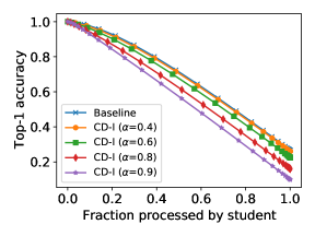
(a) Overall accuracy

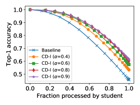
(b) In-domain accuracy

Figure 5: Comparison of various class-specific distillation methods on (subset of) ImageNet-21k. As described in Sec. D, we work with a subset corresponding to 17,203 out of 21,843 classes. Baseline denotes the standard distillation from (3) with $a=0$ and $b=1$. ${\rm CD}$-I denote the class-specific distillation approaches defined in Sec. 4.1. with $|\mathcal{L}_{\rm in}|=L^{\prime}=1000$. Accordingly, in-domain accuracy is computed via focusing on the test instances from the $1000$ classes in $\mathcal{L}_{\rm in}$. Here, each lite student model (a MobileNetV3-0.75 model) employs margin-based delegation.

Margin-based distillation with margin-based delegation.  Here, we study both overall and in-domain performance of two-stage inference enabled by margin-based distillation from Sec. 4.2 on both CIFAR-100 (cf. Fig. 6) and ImageNet (cf. Fig. 7). Here, in-domain instances correspond to those instances where the student assigns a margin of at least $\rho=0.4$. As evident, margin-based distillation also leads to improved in-domain two-stage accuracy. However, Baseline and MD from (17) have very similar performance on both datasets.

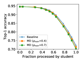
(a) Overall accuracy

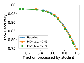
(b) In-domain accuracy

Figure 6: Performance of two-stage inference procedure enabled by the margin-based distillation approach from Sec. 4.2 on CIFAR-100. Again, Baseline denotes the standard distillation from (3) with $a=0$ and $b=1$. MD represent the margin-based distillation approach from (17). Here, each lite student model (a ResNet-32 model) employs margin-based delegation. In-domain accuracy is computed on the test instances where student achieves a margin $\rho$ of at least 0.4.

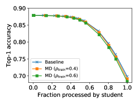
(a) Overall accuracy

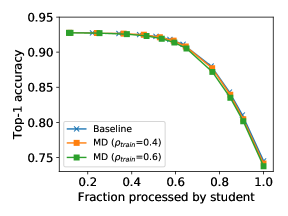
(b) In-domain accuracy

Figure 7: Performance of two-stage inference procedure enabled by the margin-based distillation approach from Sec. 4.2 on ImageNet. Here, each lite student model (a MobileNetV3-0.75 model) employs margin-based delegation. In-domain accuracy is computed on the test instances where student achieves a margin $\rho$ of at least 0.4.

References

- Bapna and Firat [2019] Ankur Bapna and Orhan Firat. Exploring massively multilingual, massive neural machine translation. In Google AI Blog, Oct 2019. URL https://ai.googleblog.com/2019/10/exploring-massively-multilingual.html.
- Bapna et al. [2020] Ankur Bapna, Naveen Arivazhagan, and Orhan Firat. Controlling computation versus quality for neural sequence models. arXiv preprint arXiv:2002.07106, 2020.
- Bartlett and Wegkamp [2008] Peter L. Bartlett and Marten H. Wegkamp. Classification with a reject option using a hinge loss. J. Mach. Learn. Res., 9:1823–1840, June 2008. ISSN 1532-4435.
- Bolukbasi et al. [2017] Tolga Bolukbasi, Joseph Wang, Ofer Dekel, and Venkatesh Saligrama. Adaptive neural networks for efficient inference. In Proceedings of the 34th International Conference on Machine Learning - Volume 70, ICML’17, page 527–536. JMLR.org, 2017.
- Brown et al. [2020] Tom Brown, Benjamin Mann, Nick Ryder, Melanie Subbiah, Jared D Kaplan, Prafulla Dhariwal, Arvind Neelakantan, Pranav Shyam, Girish Sastry, Amanda Askell, Sandhini Agarwal, Ariel Herbert-Voss, Gretchen Krueger, Tom Henighan, Rewon Child, Aditya Ramesh, Daniel Ziegler, Jeffrey Wu, Clemens Winter, Chris Hesse, Mark Chen, Eric Sigler, Mateusz Litwin, Scott Gray, Benjamin Chess, Jack Clark, Christopher Berner, Sam McCandlish, Alec Radford, Ilya Sutskever, and Dario Amodei. Language models are few-shot learners. In H. Larochelle, M. Ranzato, R. Hadsell, M. F. Balcan, and H. Lin, editors, Advances in Neural Information Processing Systems, volume 33, pages 1877–1901. Curran Associates, Inc., 2020. URL https://proceedings.neurips.cc/paper/2020/file/1457c0d6bfcb4967418bfb8ac142f64a-Paper.pdf.
- Bucilǎ et al. [2006] Cristian Bucilǎ, Rich Caruana, and Alexandru Niculescu-Mizil. Model compression. In Proceedings of the 12th ACM SIGKDD International Conference on Knowledge Discovery and Data Mining, KDD ’06, pages 535–541, New York, NY, USA, 2006. ACM.
- Cao et al. [2019] Kaidi Cao, Colin Wei, Adrien Gaidon, Nikos Arechiga, and Tengyu Ma. Learning imbalanced datasets with label-distribution-aware margin loss. In Advances in Neural Information Processing Systems, 2019.
- Carreira-Perpinán [2017] Miguel A Carreira-Perpinán. Model compression as constrained optimization, with application to neural nets. part i: General framework. arXiv preprint arXiv:1707.01209, 2017.
- Cho and Hariharan [2019] Jang Hyun Cho and Bharath Hariharan. On the efficacy of knowledge distillation. In Proceedings of the IEEE/CVF International Conference on Computer Vision, pages 4794–4802, 2019.
- Chung et al. [2016] Junyoung Chung, Sungjin Ahn, and Yoshua Bengio. Hierarchical multiscale recurrent neural networks. arXiv preprint arXiv:1609.01704, 2016.
- Cortes et al. [2016] Corinna Cortes, Giulia DeSalvo, and Mehryar Mohri. Boosting with abstention. In D. Lee, M. Sugiyama, U. Luxburg, I. Guyon, and R. Garnett, editors, Advances in Neural Information Processing Systems, volume 29, pages 1660–1668. Curran Associates, Inc., 2016.
- Crankshaw et al. [2017] Daniel Crankshaw, Xin Wang, Giulio Zhou, Michael J. Franklin, Joseph E. Gonzalez, and Ion Stoica. Clipper: A low-latency online prediction serving system. In Proceedings of the 14th USENIX Conference on Networked Systems Design and Implementation, NSDI’17, page 613–627, USA, 2017. USENIX Association. ISBN 9781931971379.
- Cui et al. [2019] Yin Cui, Menglin Jia, Tsung-Yi Lin, Yang Song, and Serge Belongie. Class-balanced loss based on effective number of samples. In CVPR, 2019.
- Dabre et al. [2020] Raj Dabre, Raphael Rubino, and Atsushi Fujita. Balancing cost and benefit with tied-multi transformers. In Proceedings of the Fourth Workshop on Neural Generation and Translation, pages 24–34, Online, July 2020. Association for Computational Linguistics. doi: 10.18653/v1/2020.ngt-1.3. URL https://www.aclweb.org/anthology/2020.ngt-1.3.
- Deng et al. [2009] Jia Deng, Wei Dong, Richard Socher, Li-Jia Li, Kai Li, and Li Fei-Fei. Imagenet: A large-scale hierarchical image database. In 2009 IEEE Conference on Computer Vision and Pattern Recognition, pages 248–255, 2009. doi: 10.1109/CVPR.2009.5206848.
- Elbayad et al. [2020] Maha Elbayad, Jiatao Gu, Edouard Grave, and Michael Auli. Depth-adaptive transformer. In International Conference on Learning Representations, 2020. URL https://openreview.net/forum?id=SJg7KhVKPH.
- Fan et al. [2019] Angela Fan, Edouard Grave, and Armand Joulin. Reducing transformer depth on demand with structured dropout. arXiv preprint arXiv:1909.11556, 2019.
- Fang et al. [2019] Zhou Fang, Dezhi Hong, and Rajesh K. Gupta. Serving deep neural networks at the cloud edge for vision applications on mobile platforms. In Proceedings of the 10th ACM Multimedia Systems Conference, MMSys ’19, page 36–47, New York, NY, USA, 2019. Association for Computing Machinery. ISBN 9781450362979. doi: 10.1145/3304109.3306221. URL https://doi.org/10.1145/3304109.3306221.
- [19] William Fedus, Barret Zoph, and Noam Shazeer. Switch transformers: Scaling to trillion parameter models with simple and efficient sparsity. arXiv preprint arXiv:2101.03961.
- Foret et al. [2021] Pierre Foret, Ariel Kleiner, Hossein Mobahi, and Behnam Neyshabur. Sharpness-aware minimization for efficiently improving generalization. In International Conference on Learning Representations, 2021. URL https://openreview.net/forum?id=6Tm1mposlrM.
- Furlanello et al. [2018] Tommaso Furlanello, Zachary Chase Lipton, Michael Tschannen, Laurent Itti, and Anima Anandkumar. Born-again neural networks. In Proceedings of the 35th International Conference on Machine Learning, ICML 2018, pages 1602–1611, 2018.
- Ganesh et al. [2020] Prakhar Ganesh, Yao Chen, Xin Lou, Mohammad Ali Khan, Yin Yang, Deming Chen, Marianne Winslett, Hassan Sajjad, and Preslav Nakov. Compressing large-scale transformer-based models: A case study on bert. arXiv preprint arXiv:2002.11985, 2020.
- Geifman and El-Yaniv [2017] Yonatan Geifman and Ran El-Yaniv. Selective classification for deep neural networks. In Proceedings of the 31st International Conference on Neural Information Processing Systems, NIPS’17, page 4885–4894, Red Hook, NY, USA, 2017. Curran Associates Inc. ISBN 9781510860964.
- Ghiasi et al. [2020] Golnaz Ghiasi, Yin Cui, Aravind Srinivas, Rui Qian, Tsung-Yi Lin, Ekin D Cubuk, Quoc V Le, and Barret Zoph. Simple copy-paste is a strong data augmentation method for instance segmentation. arXiv preprint arXiv:2012.07177, 2020.
- Gordon et al. [2020] Mitchell Gordon, Kevin Duh, and Nicholas Andrews. Compressing BERT: Studying the effects of weight pruning on transfer learning. In Proceedings of the 5th Workshop on Representation Learning for NLP, pages 143–155, Online, July 2020. Association for Computational Linguistics. doi: 10.18653/v1/2020.repl4nlp-1.18. URL https://www.aclweb.org/anthology/2020.repl4nlp-1.18.
- Grandvalet et al. [2009] Yves Grandvalet, Alain Rakotomamonjy, Joseph Keshet, and Stéphane Canu. Support vector machines with a reject option. In D. Koller, D. Schuurmans, Y. Bengio, and L. Bottou, editors, Advances in Neural Information Processing Systems, volume 21, pages 537–544. Curran Associates, Inc., 2009.
- Graves [2016] Alex Graves. Adaptive computation time for recurrent neural networks. arXiv preprint arXiv:1603.08983, 2016.
- Han et al. [2015] Song Han, Huizi Mao, and William J Dally. Deep compression: Compressing deep neural networks with pruning, trained quantization and huffman coding. arXiv preprint arXiv:1510.00149, 2015.
- Hassibi and Stork [1993] Babak Hassibi and David G Stork. Second order derivatives for network pruning: Optimal brain surgeon. Morgan Kaufmann, 1993.
- He et al. [2016a] Kaiming He, Xiangyu Zhang, Shaoqing Ren, and Jian Sun. Deep residual learning for image recognition. In Proceedings of the IEEE Conference on Computer Vision and Pattern Recognition (CVPR), June 2016a.
- He et al. [2016b] Kaiming He, Xiangyu Zhang, Shaoqing Ren, and Jian Sun. Identity mappings in deep residual networks. In Bastian Leibe, Jiri Matas, Nicu Sebe, and Max Welling, editors, Computer Vision – ECCV 2016, pages 630–645, Cham, 2016b. Springer International Publishing. ISBN 978-3-319-46493-0.
- Hinton et al. [2015] Geoffrey E. Hinton, Oriol Vinyals, and Jeffrey Dean. Distilling the knowledge in a neural network. CoRR, abs/1503.02531, 2015.
- Howard et al. [2019] Andrew Howard, Mark Sandler, Grace Chu, Liang-Chieh Chen, Bo Chen, Mingxing Tan, Weijun Wang, Yukun Zhu, Ruoming Pang, Vijay Vasudevan, Quoc V. Le, and Hartwig Adam. Searching for mobilenetv3. In Proceedings of the IEEE/CVF International Conference on Computer Vision (ICCV), October 2019.
- Huang et al. [2018] Yanping Huang, Youlong Cheng, Ankur Bapna, Orhan Firat, Mia Xu Chen, Dehao Chen, HyoukJoong Lee, Jiquan Ngiam, Quoc V Le, Yonghui Wu, et al. Gpipe: Efficient training of giant neural networks using pipeline parallelism. arXiv preprint arXiv:1811.06965, 2018.
- Jouppi et al. [2017] N. P. Jouppi, C. Young, N. Patil, D. Patterson, G. Agrawal, R. Bajwa, S. Bates, S. Bhatia, and N. Boden et al. In-datacenter performance analysis of a tensor processing unit. In 2017 ACM/IEEE 44th Annual International Symposium on Computer Architecture (ISCA), pages 1–12, Los Alamitos, CA, USA, jun 2017. IEEE Computer Society. doi: 10.1145/3079856.3080246. URL https://doi.ieeecomputersociety.org/10.1145/3079856.3080246.
- Kang et al. [2020] Bingyi Kang, Saining Xie, Marcus Rohrbach, Zhicheng Yan, Albert Gordo, Jiashi Feng, and Yannis Kalantidis. Decoupling representation and classifier for long-tailed recognition. In Eighth International Conference on Learning Representations (ICLR), 2020.
- Kolesnikov et al. [2019] Alexander Kolesnikov, Lucas Beyer, Xiaohua Zhai, Joan Puigcerver, Jessica Yung, Sylvain Gelly, and Neil Houlsby. Big transfer (bit): General visual representation learning. arXiv preprint arXiv:1912.11370, 6(2):8, 2019.
- Kovaleva et al. [2019] Olga Kovaleva, Alexey Romanov, Anna Rogers, and Anna Rumshisky. Revealing the dark secrets of bert. arXiv preprint arXiv:1908.08593, 2019.
- Krizhevsky [2009] Alex Krizhevsky. Learning multiple layers of features from tiny images. Technical report, 2009.
- LeCun et al. [1989] Yann LeCun, John S Denker, Sara A Solla, Richard E Howard, and Lawrence D Jackel. Optimal brain damage. In NIPs, volume 2, pages 598–605. Citeseer, 1989.
- Li et al. [2020] Zhuohan Li, Eric Wallace, Sheng Shen, Kevin Lin, Kurt Keutzer, Dan Klein, and Joey Gonzalez. Train big, then compress: Rethinking model size for efficient training and inference of transformers. In Hal Daumé III and Aarti Singh, editors, Proceedings of the 37th International Conference on Machine Learning, volume 119 of Proceedings of Machine Learning Research, pages 5958–5968. PMLR, 13–18 Jul 2020. URL http://proceedings.mlr.press/v119/li20m.html.
- Liang et al. [2021] Tailin Liang, John Glossner, Lei Wang, and Shaobo Shi. Pruning and quantization for deep neural network acceleration: A survey. arXiv preprint arXiv:2101.09671, 2021.
- Liu et al. [2020] Weijie Liu, Peng Zhou, Zhiruo Wang, Zhe Zhao, Haotang Deng, and Qi Ju. FastBERT: a self-distilling BERT with adaptive inference time. In Proceedings of the 58th Annual Meeting of the Association for Computational Linguistics, pages 6035–6044, Online, July 2020. Association for Computational Linguistics. doi: 10.18653/v1/2020.acl-main.537. URL https://www.aclweb.org/anthology/2020.acl-main.537.
- Liu et al. [2019] Yinhan Liu, Myle Ott, Naman Goyal, Jingfei Du, Mandar Joshi, Danqi Chen, Omer Levy, Mike Lewis, Luke Zettlemoyer, and Veselin Stoyanov. RoBERTa: A robustly optimized bert pretraining approach. arXiv preprint arXiv:1907.11692, 2019.
- Menon et al. [2020a] Aditya Krishna Menon, Ankit Singh Rawat, Sashank J. Reddi, Seungyeon Kim, and Sanjiv Kumar. Why distillation helps: a statistical perspective. CoRR, abs/2005.10419, 2020a. URL https://arxiv.org/abs/2005.10419.
- Menon et al. [2020b] Aditya Krishna Menon, Ankit Singh Rawat, Sashank J Reddi, Seungyeon Kim, and Sanjiv Kumar. Why distillation helps: a statistical perspective. arXiv preprint arXiv:2005.10419, 2020b.
- Menon et al. [2021] Aditya Krishna Menon, Sadeep Jayasumana, Ankit Singh Rawat, Himanshu Jain, Andreas Veit, and Sanjiv Kumar. Long-tail learning via logit adjustment. In International Conference on Learning Representations, 2021. URL https://openreview.net/forum?id=37nvvqkCo5.
- Mirzadeh et al. [2020] Seyed Iman Mirzadeh, Mehrdad Farajtabar, Ang Li, Nir Levine, Akihiro Matsukawa, and Hassan Ghasemzadeh. Improved knowledge distillation via teacher assistant. In Proceedings of the AAAI Conference on Artificial Intelligence, volume 34, pages 5191–5198, 2020.
- Mozer and Smolensky [1988] Michael C Mozer and Paul Smolensky. Skeletonization: A technique for trimming the fat from a network via relevance assessment. In Proceedings of the 1st International Conference on Neural Information Processing Systems, pages 107–115, 1988.
- Müller et al. [2019] Rafael Müller, Simon Kornblith, and Geoffrey E Hinton. When does label smoothing help? In H. Wallach, H. Larochelle, A. Beygelzimer, F. dAlché Buc, E. Fox, and R. Garnett, editors, Advances in Neural Information Processing Systems, volume 32. Curran Associates, Inc., 2019. URL https://proceedings.neurips.cc/paper/2019/file/f1748d6b0fd9d439f71450117eba2725-Paper.pdf.
- Ni et al. [2019] Chenri Ni, Nontawat Charoenphakdee, Junya Honda, and Masashi Sugiyama. On the calibration of multiclass classification with rejection. In H. Wallach, H. Larochelle, A. Beygelzimer, F. dAlché Buc, E. Fox, and R. Garnett, editors, Advances in Neural Information Processing Systems, volume 32, pages 2586–2596. Curran Associates, Inc., 2019.
- Ning [2013] Emma Ning. Microsoft open sources breakthrough optimizations for transformer inference on GPU and CPU. https://cloudblogs.microsoft.com/opensource/2020/01/21/microsoft-onnx-open-source-optimizations-transformer-inference-gpu-cpu/, 2013. Online; accessed 17 March 2021.
- Raffel et al. [2019] Colin Raffel, Noam Shazeer, Adam Roberts, Katherine Lee, Sharan Narang, Michael Matena, Yanqi Zhou, Wei Li, and Peter J Liu. Exploring the limits of transfer learning with a unified text-to-text transformer. arXiv preprint arXiv:1910.10683, 2019.
- Raganato et al. [2020] Alessandro Raganato, Yves Scherrer, and Jörg Tiedemann. Fixed encoder self-attention patterns in transformer-based machine translation. arXiv preprint arXiv:2002.10260, 2020.
- Rajpurkar et al. [2016] Pranav Rajpurkar, Jian Zhang, Konstantin Lopyrev, and Percy Liang. SQuAD: 100,000+ questions for machine comprehension of text. In Proceedings of the 2016 Conference on Empirical Methods in Natural Language Processing, pages 2383–2392, Austin, Texas, November 2016. Association for Computational Linguistics. doi: 10.18653/v1/D16-1264. URL https://www.aclweb.org/anthology/D16-1264.
- Ramaswamy et al. [2018] Harish G. Ramaswamy, Ambuj Tewari, and Shivani Agarwal. Consistent algorithms for multiclass classification with an abstain option. Electron. J. Statist., 12(1):530–554, 2018. doi: 10.1214/17-EJS1388. URL https://doi.org/10.1214/17-EJS1388.
- Romero et al. [2014] Adriana Romero, Nicolas Ballas, Samira Ebrahimi Kahou, Antoine Chassang, Carlo Gatta, and Yoshua Bengio. Fitnets: Hints for thin deep nets. arXiv preprint arXiv:1412.6550, 2014.
- Rowley et al. [1998] H. A. Rowley, S. Baluja, and T. Kanade. Neural network-based face detection. IEEE Transactions on Pattern Analysis and Machine Intelligence, 20(1):23–38, 1998. doi: 10.1109/34.655647.
- Russakovsky et al. [2015] Olga Russakovsky, Jia Deng, Hao Su, Jonathan Krause, Sanjeev Satheesh, Sean Ma, Zhiheng Huang, Andrej Karpathy, Aditya Khosla, Michael Bernstein, Alexander C. Berg, and Li Fei-Fei. ImageNet Large Scale Visual Recognition Challenge. International Journal of Computer Vision (IJCV), 115(3):211–252, 2015. doi: 10.1007/s11263-015-0816-y.
- Rusu et al. [2016] Andrei A. Rusu, Sergio Gomez Colmenarejo, Çaglar Gülçehre, Guillaume Desjardins, James Kirkpatrick, Razvan Pascanu, Volodymyr Mnih, Koray Kavukcuoglu, and Raia Hadsell. Policy distillation. In 4th International Conference on Learning Representations, ICLR 2016, 2016.
- Schwartz et al. [2020] Roy Schwartz, Gabriel Stanovsky, Swabha Swayamdipta, Jesse Dodge, and Noah A. Smith. The right tool for the job: Matching model and instance complexities. In Proceedings of the 58th Annual Meeting of the Association for Computational Linguistics, pages 6640–6651, Online, July 2020. Association for Computational Linguistics. doi: 10.18653/v1/2020.acl-main.593. URL https://www.aclweb.org/anthology/2020.acl-main.593.
- Sun et al. [2017] C. Sun, A. Shrivastava, S. Singh, and A. Gupta. Revisiting unreasonable effectiveness of data in deep learning era. In 2017 IEEE International Conference on Computer Vision (ICCV), pages 843–852, 2017. doi: 10.1109/ICCV.2017.97.
- Sun et al. [2020] Zhiqing Sun, Hongkun Yu, Xiaodan Song, Renjie Liu, Yiming Yang, and Denny Zhou. MobileBERT: a compact task-agnostic BERT for resource-limited devices. In Proceedings of the 58th Annual Meeting of the Association for Computational Linguistics, pages 2158–2170, Online, July 2020. Association for Computational Linguistics. doi: 10.18653/v1/2020.acl-main.195. URL https://www.aclweb.org/anthology/2020.acl-main.195.
- Szegedy et al. [2016] Christian Szegedy, Vincent Vanhoucke, Sergey Ioffe, Jon Shlens, and Zbigniew Wojna. Rethinking the inception architecture for computer vision. In Proceedings of the IEEE Conference on Computer Vision and Pattern Recognition (CVPR), June 2016.
- Tan and Le [2019] Mingxing Tan and Quoc Le. EfficientNet: Rethinking model scaling for convolutional neural networks. In Kamalika Chaudhuri and Ruslan Salakhutdinov, editors, Proceedings of the 36th International Conference on Machine Learning, volume 97 of Proceedings of Machine Learning Research, pages 6105–6114. PMLR, 09–15 Jun 2019. URL http://proceedings.mlr.press/v97/tan19a.html.
- Van Horn and Perona [2017] Grant Van Horn and Pietro Perona. The devil is in the tails: Fine-grained classification in the wild. arXiv preprint arXiv:1709.01450, 2017.
- Viola and Jones [2001] P. Viola and M. Jones. Rapid object detection using a boosted cascade of simple features. In Proceedings of the 2001 IEEE Computer Society Conference on Computer Vision and Pattern Recognition. CVPR 2001, volume 1, pages I–I, 2001. doi: 10.1109/CVPR.2001.990517.
- Wang et al. [2017a] Xin Wang, Yujia Luo, Daniel Crankshaw, Alexey Tumanov, Fisher Yu, and Joseph E Gonzalez. Idk cascades: Fast deep learning by learning not to overthink. arXiv preprint arXiv:1706.00885, 2017a.
- Wang et al. [2018] Xin Wang, Fisher Yu, Zi-Yi Dou, Trevor Darrell, and Joseph E Gonzalez. Skipnet: Learning dynamic routing in convolutional networks. In Proceedings of the European Conference on Computer Vision (ECCV), pages 409–424, 2018.
- Wang et al. [2017b] Yu-Xiong Wang, Deva Ramanan, and Martial Hebert. Learning to model the tail. In Proceedings of the 31st International Conference on Neural Information Processing Systems, pages 7032–7042, 2017b.
- Williams et al. [2018] Adina Williams, Nikita Nangia, and Samuel Bowman. A broad-coverage challenge corpus for sentence understanding through inference. In Proceedings of the 2018 Conference of the North American Chapter of the Association for Computational Linguistics: Human Language Technologies, Volume 1 (Long Papers), pages 1112–1122, New Orleans, Louisiana, June 2018. Association for Computational Linguistics. doi: 10.18653/v1/N18-1101. URL https://aclanthology.org/N18-1101.
- Xie et al. [2020] Qizhe Xie, Minh-Thang Luong, Eduard Hovy, and Quoc V. Le. Self-training with noisy student improves imagenet classification. In Proceedings of the IEEE/CVF Conference on Computer Vision and Pattern Recognition (CVPR), June 2020.
- Xu et al. [2014] Zhixiang (Eddie) Xu, Matt J. Kusner, Kilian Q. Weinberger, Minmin Chen, and Olivier Chapelle. Classifier cascades and trees for minimizing feature evaluation cost. Journal of Machine Learning Research, 15(62):2113–2144, 2014. URL http://jmlr.org/papers/v15/xu14a.html.
- Yuan et al. [2020] Li Yuan, Francis EH Tay, Guilin Li, Tao Wang, and Jiashi Feng. Revisiting knowledge distillation via label smoothing regularization. In Proceedings of the IEEE/CVF Conference on Computer Vision and Pattern Recognition (CVPR), June 2020.
- Zadeh et al. [2020] Ali Hadi Zadeh, Isak Edo, Omar Mohamed Awad, and Andreas Moshovos. Gobo: Quantizing attention-based nlp models for low latency and energy efficient inference. In 2020 53rd Annual IEEE/ACM International Symposium on Microarchitecture (MICRO), pages 811–824. IEEE, 2020.
- Zhang et al. [2020] Mi Zhang, Faen Zhang, Nicholas D Lane, Yuanchao Shu, Xiao Zeng, Biyi Fang, Shen Yan, and Hui Xu. Deep learning in the era of edge computing: Challenges and opportunities. Fog Computing: Theory and Practice, pages 67–78, 2020.
- Zhang et al. [2019] Minjia Zhang, Samyam Rajbandari, Wenhan Wang, Elton Zheng, Olatunji Ruwase, Jeff Rasley, Jason Li, Junhua Wang, and Yuxiong He. Accelerating large scale deep learning inference through deepcpu at microsoft. In 2019 USENIX Conference on Operational Machine Learning (OpML 19), pages 5–7, Santa Clara, CA, May 2019. USENIX Association. ISBN 978-1-939133-00-7. URL https://www.usenix.org/conference/opml19/presentation/zhang-minjia.
- Zhu et al. [2014] Xiangxin Zhu, Dragomir Anguelov, and Deva Ramanan. Capturing long-tail distributions of object subcategories. In Proceedings of the IEEE Conference on Computer Vision and Pattern Recognition, pages 915–922, 2014.