Purely Radiative Higgs Mass in Scale invariant models

Abstract

In this work, we investigate the possibility of having scale invariant (SI) standard model (SM) extensions, where the light CP-even scalar matches the SM-like Higgs instead of being a light dilaton. After deriving the required conditions for this scenario, we show that the radiative corrections that give rise to the Higgs mass can trigger the scalar mixing to the experimentally allowed values. In addition, we discuss the constraints on the parameters space that makes the CP-even scalars properties in a good agreement with all the recent ATLAS and CMS measurements. We illustrate this scenario by considering the SI-scotogenic model as an example, while imposing all the theoretical and experimental constraints. We show that the model is viable and leads to possible modifications of the di-Higgs signatures at current/future with respect to the SM.

Keywords: classical scale invariance, Higgs mass & heavy scalar resonance.

I Introduction

Despite the Higgs discovery ATLAS:2012yve , many questions are still open within the standard model (SM), among them understanding the origin of the Higgs mass. It is well known that in the SM, the quadratic divergences appear in the radiative corrections to the Higgs mass, which cause what is called the hierarchy problem. It is widely believed that some possible solutions to the hierarchy problem come with a classically conformally invariant action at a higher energy scale that is below the gravity (Planck) scale, despite the fact that any gravity theory is not conformally scale invariant due to the presence of Planck mass as a dimensionful parameter Meissner:2006zh . Since we do not know yet the gravity theory, one can assume the classical SI invariance up to a scale below Planck by making the quadratic Higgs mass term in the Lagrangian is set to zero ($\mu^{2}=0$). In this setup, the electroweak symmetry breaking (EWSB) occurs via the so-called dimensional transmutation, where the scale invariance symmetry is broken at the quantum level Coleman:1973jx .

The SI symmetry breaking is associated by a pseudo-Goldstone boson (PGB) that is strictly massless at tree-level; and acquires its mass via the radiative corrections. This light scalar is called the “dilaton” scalar in the literature. The realization of the EWSB a la Coleman-Weinberg within some SM popular extensions has been extensively discussed in the literature (for example, see Alexander-Nunneley:2010tyr ). Although, many models are SI extended to address to the hierarchy problem, in addition to other problems such as the dark matter (DM) and the neutrino oscillation data Foot:2007ay ; Ahriche:2016cio . Here, we aim to investigate the case where the light PGB is the observed $125~{}\mathrm{GeV}$ SM-like Higgs rather than a light dilaton. It has been shown in the literature Bellazzini:2012vz ; Foot:2007as , that the case of a dilaton-like Higgs, or a purely radiative mass Higgs (PRMH) is possible, however, the requirements for such case were not discussed, as well the agreement with the recent LHC measurements relevant to the scalar sector.

In this work, we consider a generic SI model, where the SM is extended by a real scalar singlet to assist the EWSB, in addition to new scalar and fermionic field representations. In this general setup, we investigate the EWSB and define the required conditions to have a PRMH case. Then, we show how should this setup be in agreement with all the Higgs measurements ATLAS:2016neq ; and the negative searches for a heavy resonance ATLAS:2020zms ; ATLAS:2020tlo ; CMS:2021klu ; ATLAS:2021nps ; ATLAS:2021fet ; ATLAS:2021ulo ; ATLAS:2021jki . As will be shown later, the radiative corrections due to the interactions of the new scalar and fermionic fields to the SM Higgs doublet and the real singlet; could play a key role. As they give rise to the Higgs mass, they are also responsible to adjust the scalar mixing to be in agreement with the recent constraints; and fully control some triple scalar couplings that can be directly probed through the di-Higgs production at both LHC and ILC. In order to illustrate our discussion, we consider a phenomenologically rich SI model Ahriche:2016cio as an example.

This work is organized as follow: in section II, we discuss the EWSB and deduce the required conditions for a PRMH case is section III. Then, the experimental constraints and the predictions at colliders are investigated in section IV. Section V is devoted for an illustrative example and our conclusions are summarized in section VI.

II The EWBS in SI Models

The classical scale invariance symmetry enforces the action to be invariant under the conformal transformation $\Phi_{i}(x^{\mu})\rightarrow e^{a~{}\kappa}\,\Phi_{i}(e^{\kappa}\,x^{\mu})$, which implies the vanishing of the scalar quadratic and the fermionic mass terms in the Lagrangian density. Then, for a model with many scalar representations, the scalar potential can be written in the general form

$$V=\sum_{i,j,k,l}\lambda_{ijkl}\Phi_{i}\Phi_{j}\Phi_{k}\Phi_{l},$$ (1)

where the couplings $\lambda_{ijkl}$ are not vanishing due to the symmetries that are assigned to the model. Generally, most of the SI models in the literature include the SM Higgs doublet $\mathcal{H}^{T}=\Big{(}\chi^{+},~{}[h+i~{}\chi^{0}]/\sqrt{2}\Big{)}$, a real scalar singlet $\phi$ to assists the EWSB in addition to other bosonic and fermionic representations with different multiplicities. After the EWSB, the CP-even neutral scalars acquire their VEV’s as

$$\mathcal{H}\rightarrow\frac{\upsilon+h}{\sqrt{2}}\begin{pmatrix}0\\ 1\end{pmatrix},\,\,\,\phi\rightarrow x+\phi,$$ (2)

and give masses to all the model fields. Then, we get two CP-even eigenstates $h_{1,2}$ ($m_{1}<m_{2}$) via a rotation with the angle $\alpha$ in the basis {$h,\phi$}, where one of the eigenstates must match the SM-like Higgs with the measured mass $m_{h}=125.18\,\mathrm{GeV}$. In the literature, the heavier eigenstate $h_{2}=H$ corresponds to the SM-like Higgs and $h_{1}=D$ is the dilaton scalar, that is strictly massless at tree-level and acquires its mass via the radiative corrections. The other case corresponds to a purely radiative mass Higgs (PRMH) scenario, i.e., $h_{1}=H$ and $h_{2}=S$ would be a heavy CP-even scalar. The aim of this work is to investigate the viability of the PRMH scenario and to show possible interesting signatures at colliders.

In order to achieve the EWSB, one has to consider the radiative corrections to the scalar potential. The one-loop effective scalar potential can be written in function of the CP-even scalar fields as

$$V^{1-\ell}(h,\phi) = \frac{1}{24}(\lambda_{h}+\delta\lambda_{h})h^{4}+\frac{1}{24}(\lambda_{\phi}+\delta\lambda_{\phi})\phi^{4}+\frac{1}{4}(\omega+\delta\omega)h^{2}\,\phi^{2}+\sum_{i}n_{i}G\Big{(}m_{i}^{2}\Big{)},$$ (3)

where $\delta\lambda_{h},\,\delta\lambda_{\phi}$ and $\delta\omega$ are the counter-terms, $n_{i}$ and $m_{i}^{2}\equiv m_{i}^{2}(h,\phi)$ are the field multiplicities and field dependent squared masses. Here, the function $G(r_{i})=\frac{r_{i}^{2}}{64\pi^{2}}\Big{(}\log\frac{r_{i}}{\Lambda^{2}}-c_{i}\Big{)}$ is defined a la the $\overline{DR}$ scheme ($c_{i}=3/2$) and $\Lambda$ is the renormalization scale. The appearance of the dimensionful parameter $\Lambda$ shows the scale invariance is broken, and when studying the phenomenology of the model, such as the physics at the colliders, it should take a value of the electroweak scale order like $\Lambda=m_{h}$.

Including the CTs is mandatory to in order cancel the divergences that appear from the one-loop corrections, and therefore regularize the theory. The way these infinities are absorbed by the CTs depends on the definition of the renormalized parameters, i.e., on the choice of the renormalization conditions. Here, in our work I adopted a modified version of the $\bar{DR}$ scheme, where the choice of the CTs (more precisely their cut-off independent parts) makes the values of the masses and mixing at tree-level and one-loop having identical values at the vacuum $\{h=\upsilon,\phi=x\}$. In other words, the CTs should be derived from the three conditions $\left.\partial V^{1-\ell}/\partial h\right|_{h=\upsilon,\phi=x}=\left.\partial V^{1-\ell}/\partial\phi\right|_{h=\upsilon,\phi=x}=0$ and the Higgs mass $m_{1,2}^{2\,(1-\ell)}=m_{h}^{2}$.

Using the tadpole conditions, the one-loop scalar squared mass matrix in the basis {$h,\phi$}, can be written in function of $\delta\omega$, as

$$\textrm{M}^{2}=\left[\frac{m_{h}^{2}}{\upsilon^{2}+x^{2}}-\delta\omega\right]\left(\begin{array}[]{cc}x^{2}&-\upsilon x\\ -\upsilon x&\upsilon^{2}\end{array}\right)+m_{h}^{2}\left(\begin{array}[]{cc}a&c\\ c&b\end{array}\right),$$ (4)

and the one-loop contributions to the Higgs/dilaton mass are characterized by the dimensionless parameters

$$a =\frac{1}{m_{h}^{2}}\sum_{i}n_{i}\left[\left(\partial_{h,h}m_{i}^{2}-\frac{3}{\upsilon}\partial_{h}m_{i}^{2}\right)G^{\prime}(m_{i}^{2})+\left(\partial_{h}m_{i}^{2}\right)^{2}G^{\prime\prime}(m_{i}^{2})\right]_{h=\upsilon,\phi=x},$$ (5)

$$b =\frac{1}{m_{h}^{2}}\sum_{i}n_{i}\left[\left(\partial_{\phi,\phi}m_{i}^{2}-\frac{3}{x}\partial_{\phi}m_{i}^{2}\right)G^{\prime}(m_{i}^{2})+\left(\partial_{\phi}m_{i}^{2}\right)^{2}G^{\prime\prime}(m_{i}^{2})\right]_{h=\upsilon,\phi=x},$$ (6)

$$c =\frac{1}{m_{h}^{2}}\sum_{i}n_{i}\left[\Big{(}\partial_{h,\phi}m_{i}^{2}\Big{)}G^{\prime}(m_{i}^{2})+(\partial_{h}m_{i}^{2})(\partial_{\phi}m_{i}^{2})G^{\prime\prime}(m_{i}^{2})\right]_{h=\upsilon,\phi=x},$$ (7)

where $G^{\prime}(r)=\partial G(r)/\partial r$, $G^{\prime\prime}(r)=\partial^{2}G(r)/\partial r^{2}$, $\partial_{x}=\frac{\partial}{\partial x}$ and $\partial_{x,y}=\frac{\partial^{2}}{\partial x\partial y}$. In order to find the value of the counter-term $\delta\omega$, we require the measured Higgs mass to match one of the eigenmasses, i.e., $2m_{h}^{2}=\textrm{M}_{11}^{2}+\textrm{M}_{22}^{2}\pm\{(\textrm{M}_{22}^{2}-\textrm{M}_{11}^{2})^{2}+4(\textrm{M}_{12}^{2})^{2}\}^{1/2}$. Both cases give the same value for $\delta\omega$,

$$\delta\omega =\frac{m_{h}^{2}}{\upsilon^{2}+x^{2}}\frac{(ab-c^{2})(\upsilon^{2}+x^{2})-ax^{2}-b\upsilon^{2}+2\,c\upsilon x}{a\upsilon^{2}+bx^{2}+2\,c\upsilon x-\upsilon^{2}-x^{2}}.$$ (8)

Numerically, the counter-terms $\delta\omega$, $\delta\lambda_{h}$ and/or $\delta\lambda_{\phi}$ may acquire large values, especially for large singlet VEV $x$, non-negligible dimensionless couplings and/or large fields multiplicities. To avoid such naturalness, one has to impose the perturbativity constraints at one-loop level. This can be achieved by considering the one-loop quartic couplings

$$\lambda_{h,\phi}^{1-\ell},\,|\omega^{1-\ell}|<4\,\pi,$$ (9)

where these one-loop couplings are defined as the $4^{th}$ derivatives of the effective potential (3) at the vacuum {$h=\upsilon,~{}\phi=x$}. Although, there is no need to impose the vacuum stability conditions at tree-level $\min[\lambda_{h},~{}\lambda_{\phi},~{}3\omega+\{\lambda_{h}\lambda_{\phi}\}^{1/2}]>0$ or at one-loop $\min[\lambda_{h}^{1-\ell},~{}\lambda_{\phi}^{1-\ell},~{}3\omega^{1-\ell}+\{\lambda_{h}^{1-\ell}\lambda_{\phi}^{1-\ell}\}^{1/2}]>0$, since the leading term in the effective potential (3) is $\varphi^{4}\log\varphi$ rather than $\varphi^{4}$, where $\varphi$ stands for any direction in the plan {$h,\phi$}. Therefore, the one-loop conditions of the vacuum stability come from the coefficients positivity of the terms $\varphi^{4}\log\varphi$ in the effective potential. In other words, we must have

$$\sum_{i}n_{i}m_{i}^{2}(h=\upsilon,\phi=0)>0,~{}~{}~{}~{}\sum_{i}n_{i}m_{i}^{2}(h=0,\phi=x)>0,$$ (10)

as the one-loop vacuum stability conditions Soualah:2021xbn . Concerning the SI breaking scale $\Lambda_{0}$, one has to estimate the RGE solution for quartic couplings; and estimate the running up to higher scale, much higher than $\Lambda=m_{h}$, then, $\Lambda_{0}$ can be defined as the scale where of the perturbativity and/or the vacuum stability conditions get broken. This depends on the model field content, multiplicities, and couplings. Such analysis about the vacuum structure at higher energy scales within the SI-scotogenic model is under investigation ahriche .

III The Purely Radiative Mass Higgs

After the EWSB, we obtain two CP-even eigenstates in the PRMH scenario as

$$\begin{pmatrix}H\\ S\end{pmatrix}=\begin{pmatrix}c_{\alpha}~{}-s_{\alpha}\\ s_{\alpha}~{}c_{\alpha}\end{pmatrix}\begin{pmatrix}h\\ \phi\end{pmatrix},$$ (11)

where $c_{\alpha}=\cos\alpha,\,s_{\alpha}=\sin\alpha$ , $H$ denotes the 125 $\mathrm{GeV}$ Higgs, $S$ is the new heavy scalar and $\alpha$ is the scalar mixing angle, that is defined by

$$\tan 2\alpha=2\textrm{M}_{12}^{2}/\Big{[}\textrm{M}_{22}^{2}-\textrm{M}_{11}^{2}\Big{]},$$ (12)

with $\textrm{M}_{ij}^{2}$ are the elements of (4).

Depending on the model free parameters (the singlet VEV $x$ and the fields couplings to the real scalar singlet and the Higgs doublet), the observed $125~{}\mathrm{GeV}$ SM-like Higgs could match the heavier (light dilaton case) or the lighter (PRHM case) CP-even eigenstate. The light dilaton case is possible only if $m_{h}^{2}<\textrm{M}_{11}^{2}+\textrm{M}_{22}^{2}<2\,m_{h}^{2}$ that can be translated into

$$\delta\omega(x^{2}+\upsilon^{2})/m_{h}^{2}<a+b<1+\delta\omega(x^{2}+\upsilon^{2})/m_{h}^{2},$$ (13)

This condition (13) ensures that the dilaton squared mass is positive and smaller than the Higgs one. The PRMH scenario is possible if $\textrm{M}_{11}^{2}+\textrm{M}_{22}^{2}>2\,m_{h}^{2}$, which leads to

$$a+b>1+\delta\omega(x^{2}+\upsilon^{2})/m_{h}^{2}.$$ (14)

In order to have an idea about the quantum corrections that lead to the PRMH scenario (i.e., fulfilling the condition (14)) compared to the light dilaton one, we consider a toy model where the SM is extended by a scalar singlet (2) to assist the EWSB; and another singlet scalar $Q$ with multiplicity $N_{Q}$ and the squared mass $m_{Q}^{2}=\frac{1}{2}(\alpha_{Q}\upsilon^{2}+\beta_{Q}x^{2})$. Clearly, the quantum corrections effect should be proportional to the field multiplicity $N_{Q}$, the couplings ($\alpha_{Q},\,\beta_{Q}$) to $\mathcal{H}$ and $\phi$ and/or the singlet VEV $x$. To confirm this, we show in Fig. 1 (Fig. 2), the parameter space ($\alpha_{Q},~{}\beta_{Q}$) for both light dilaton and PRHM cases, where the palette shows $m_{Q}$ (the mixing $s_{\alpha}$) for different values of the multiplicity $N_{Q}=6,12,24$; and the singlet VEV $x=500\,\mathrm{GeV},~{}1\,\mathrm{TeV},~{}3\,\mathrm{TeV}$. These figures are produced by taking into account the perturbativity one-loop constraints (9), in addition to the vacuum stability (10).

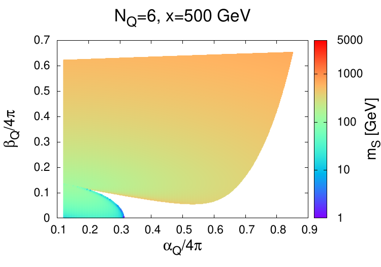
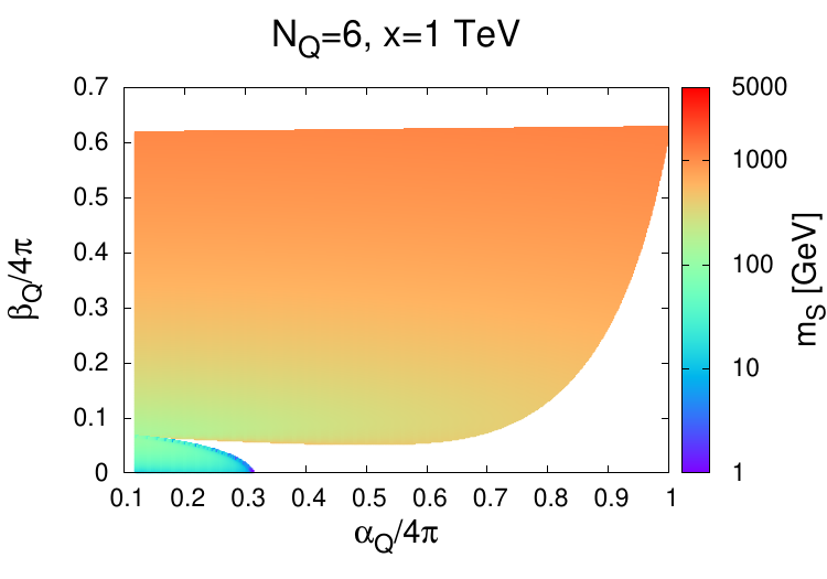
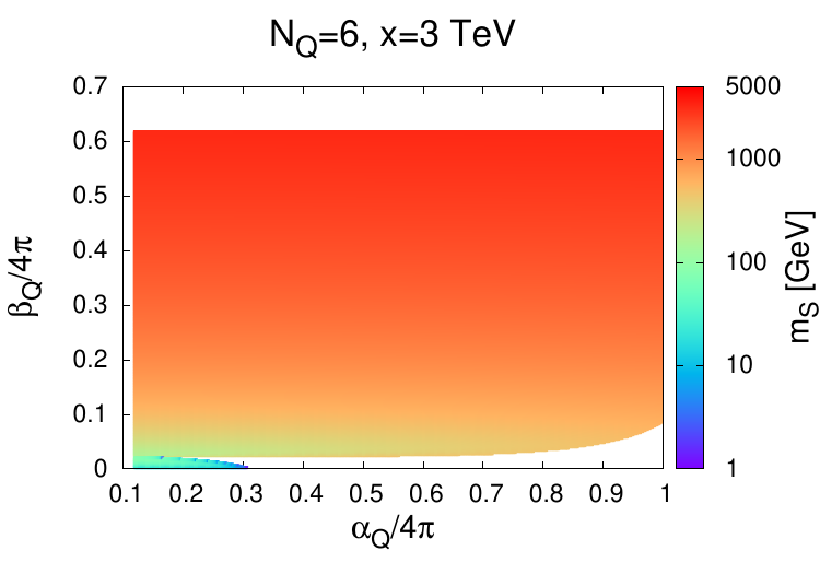
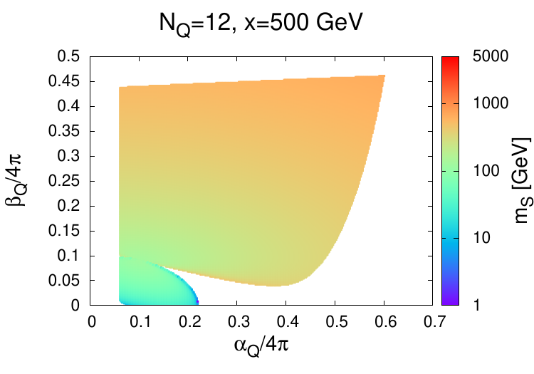
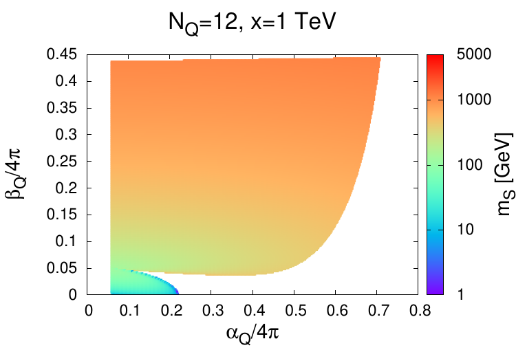
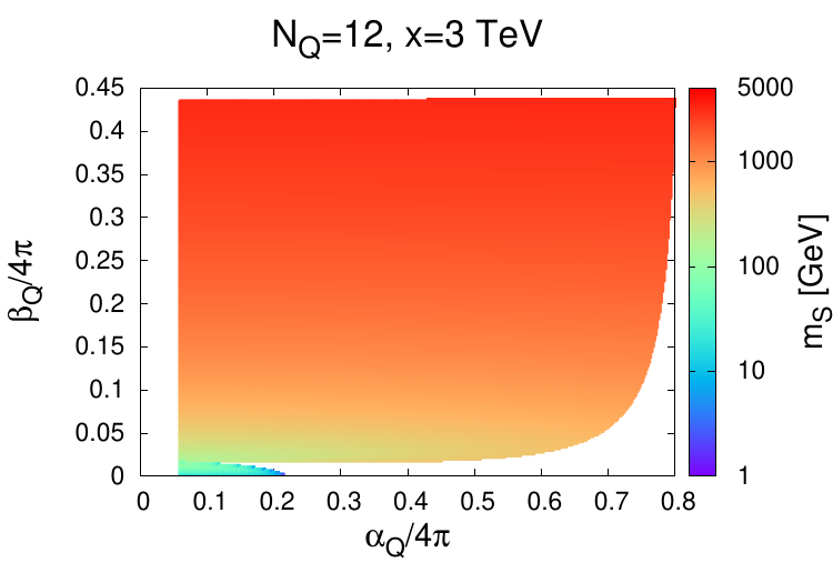
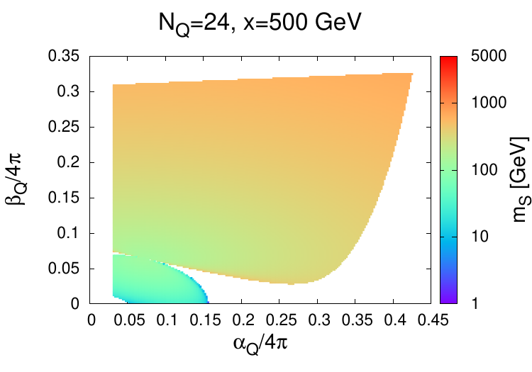
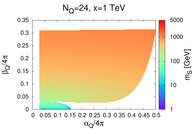
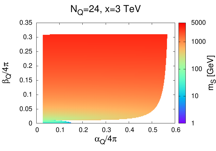
Figure 1: The couplings $\alpha_{Q}$ and $\beta_{Q}$, where the palette shows the extra scalar mass $m_{Q}$, and the one-loop perturbativity (9); and vacuum stability (10) constraints are considered. These upper larger (lower smaller) island corresponds to the PRMH (light dilaton) scenario.

From Fig. 1, one sees that in all panels there exist two islands; a lower smaller island and a larger upper one, which corresponds to the light dilaton and PRHM cases, respectively. Clearly, the parameter space in the PRHM case is much larger than the light dilaton case. Indeed, this is easy to understand since the radiative corrections (i.e., values of $N,~{},\alpha_{Q},~{}and~{}\beta_{Q}$) that are required to achieve the EWSB and make the light CP-even eigenstate matching the observed SM-like Higgs; should be much larger than case of breaking the EW symmetry and give a tiny mass to the dilaton.

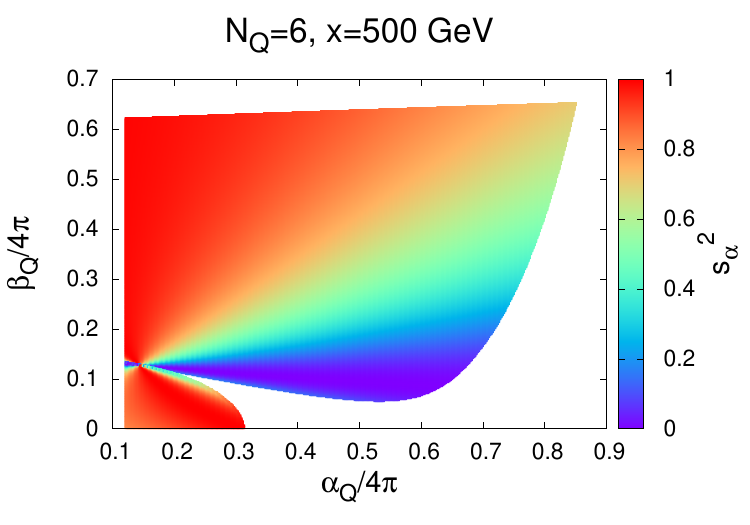
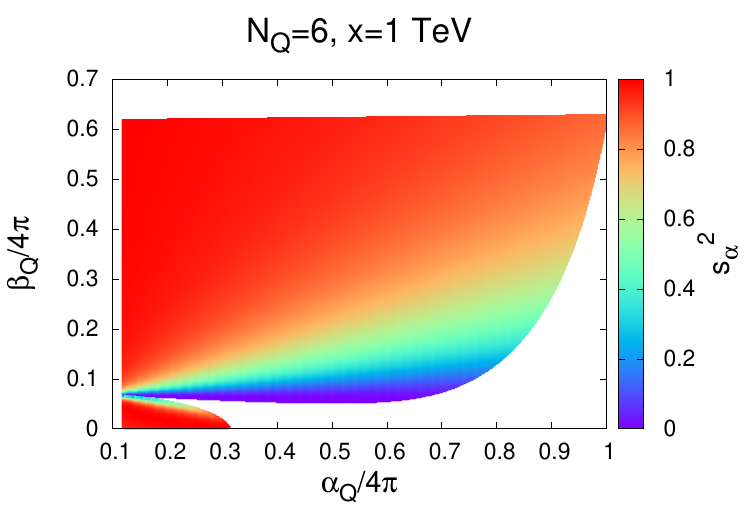
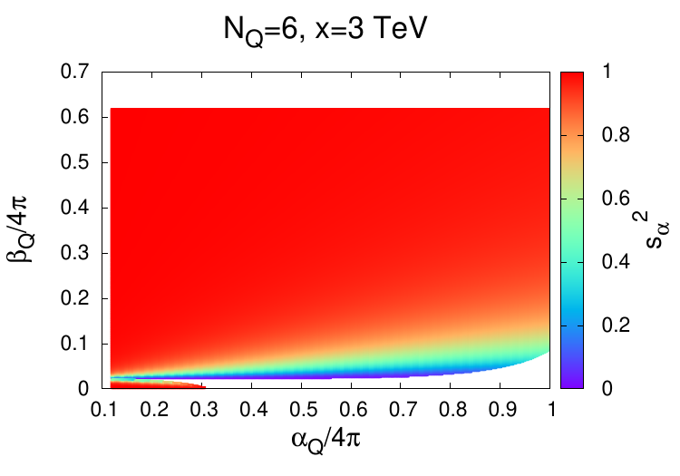
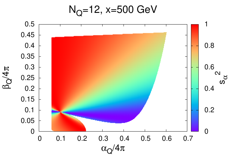
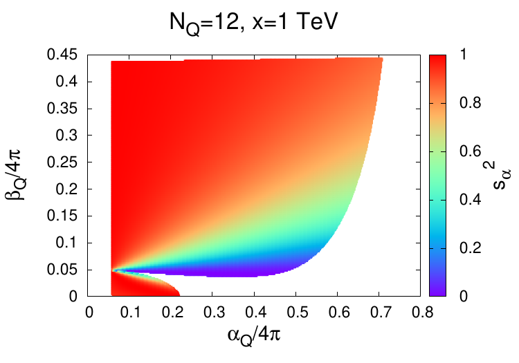
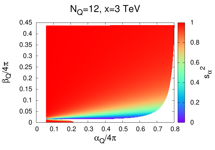
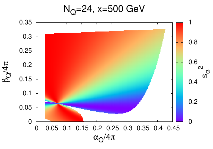
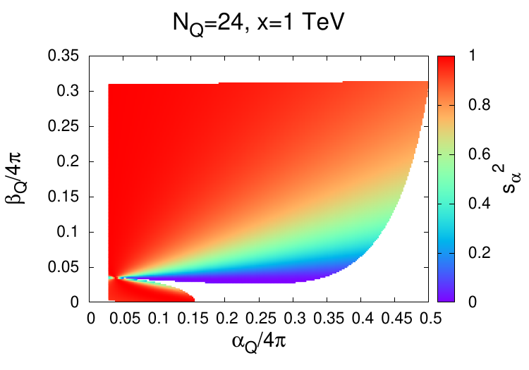
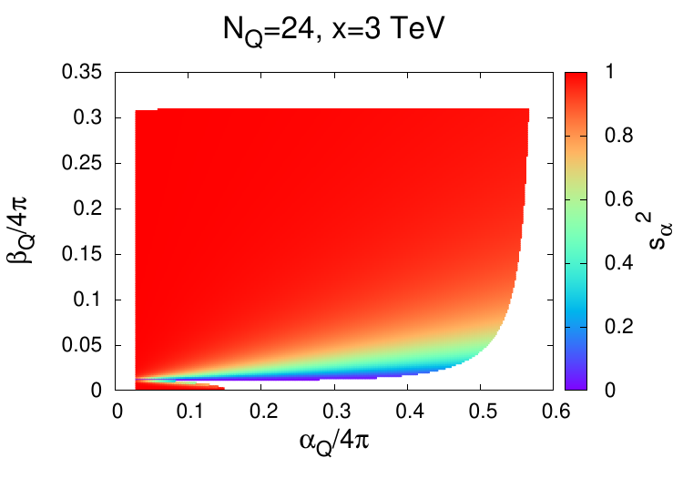
Figure 2: The couplings $\alpha_{Q}$ and $\beta_{Q}$, where the palette shows the scalar mixing $s_{\alpha}^{2}$, and the one-loop perturbativity (9); and vacuum stability (10) constraints are considered. These upper larger (lower smaller) island corresponds to the PRMH (light dilaton) scenario.

In both Fig. 1 and Fig. 2, the shape of the parameters space for different values of the singlet VEV ($x$) and the new scalar multiplicity ($N_{Q}$) is dictated by many constraints such as the positivity of $m_{Q}^{2}>0$, the one-loop perturbativity (9); the vacuum stability conditions (10); and the definition of both light dilaton and PRMH scenarios. One has to mention that the two region are connected in a point at least, which corresponds to the case of two degenerate scalars at the mass $m=125~{}\mathrm{GeV}$. This twin Higgs scenario could be of great interest Heikinheimo:2013cua .

From Fig. 1, one learns that the condition (14) can be fulfilled for small couplings ($\alpha_{Q}$, $\beta_{Q}$) and small masses. However, for larger $m_{Q}$ values, i.e., by making the singlet VEV ($x$) larger, the PRMH scenario can be achieved for larger values of the couplings ($\alpha_{Q}$, $\beta_{Q}$). It is clear that pushing the singlet VEV to higher values leads to the decoupling limit. From Fig. 2, one notices that the light green color corresponds to small scalar mixing values, that is in agreement with the experimental constraints as we will see in the next section. Obviously, it clear that for larger singlet VEV and multiplicity values, the viable parameters space is larger for the PRHM scenario. Here, one has to mention that in realistic models where many fermionic and scalar degrees of freedom and added to the SM, there will be more parameters, more freedom and more theoretical and experimental constraints, as will be seen in section V. In what follows, we will be interested in PRHM scenario.

IV Constraints & Predictions

Both ATLAS and CMS measurements at $\sqrt{s}=7+8\,\mathrm{TeV}$ reported the total Higgs signal strength modifier to be $\mu_{{\rm tot}}=c_{\alpha}^{2}\times(1-\mathcal{B}_{BSM})\geq 0.89$ at 95 % CL ATLAS:2016neq , which implies $s_{\alpha}^{2}\leq 0.11$ in the absence of invisible and undetermined Higgs decay ($\mathcal{B}_{BSM}=0$). Since the tree-level scalar mixing in the PRMH scenario is defined by $s_{\alpha}^{(0)}=-x/(\upsilon^{2}+x^{2})^{1/2}$, the bound ($(s_{\alpha}^{(0)})^{2}\leq 0.11$) leads to contradictory values for the singlet VEV $x\leq 86.6~{}\mathrm{GeV}$. Then, if one writes $s_{\alpha}=(1+\Delta_{\sin\alpha})s_{\alpha}^{(0)}$, the radiative corrections to the mixing must be large and negative

$$|1+\Delta_{\sin\alpha}|<\sqrt{0.11}(1+\upsilon^{2}/x^{2})^{1/2},$$ (15)

in order to have a viable PRMH scenario for natural values of the singlet VEV $x>\upsilon$. Therefore, the radiative effects (quantified by the fields multiplicities and couplings to the Higgs doublet and to the real singlet) must push the light CP-even scalar mass to match $m_{h}$ and give a large negative contribution to the scalar mixing sine ($s_{\alpha}$) at the same time to have a viable SM-like Higgs in the PRMH scenario. The radiative corrections to the scalar mixing (15) in this scenario are so constrained with respect to the light dilaton scenario, since the tree-level mixing $s_{\alpha}^{(0)}=\upsilon/(\upsilon^{2}+x^{2})^{1/2}$ is naturally small, and therefore allows large (positive or negative) radiative corrections $|\Delta_{\sin\alpha}|\leq 1500\%$ Soualah:2021xbn .

In the PRMH scenario, in addition to the constraints on the Higgs due to the Higgs signal strength modifiers, the di-photon, invisible and undetermined decays and the total Higgs decay width, the new heavy CP-even scalar $S$ is a subject of constraints from many negative searches at the LHC. Since the CP-even field of the Higgs doublet can be written as $h=H~{}c_{\alpha}+S~{}s_{\alpha}$, then the scalar S has the same SM-like Higgs couplings to the SM fermions and gauge bosons scaled either by $s_{\alpha}$ or $s_{\alpha}^{2}$. Hence, it decays to all the SM Higgs final states, di-Higgs final state or via other invisible or undetermined channels according to the model field content. This allows different search types among them looking for a heavy CP-even resonance in the channels of pair of leptons, jets or gauge bosons $pp\rightarrow S\rightarrow\ell\ell,jj,VV$; and the search of resonant di-Higgs production $pp\rightarrow S\rightarrow HH$. For the first type, we consider the recent ATLAS analysis at $13~{}\mathrm{TeV}$ with 139 $\mathrm{fb}^{-1}$ $pp\rightarrow S\rightarrow\tau\tau$ ATLAS:2020zms , and $pp\rightarrow S\rightarrow ZZ$ via the channels $\ell\ell\ell\ell$ and $\ell\ell\nu\nu$ ATLAS:2020tlo , in addition to the CMS analysis at $13~{}\mathrm{TeV}$ with 137 $\mathrm{fb}^{-1}$ $pp\rightarrow S\rightarrow WW$ CMS:2021klu . For the second type, we consider the recent ATLAS combination ATLAS:2021nps , that includes the analyses at $13~{}\mathrm{TeV}$ with 139 $\mathrm{fb}^{-1}$ via the channels $HH\rightarrow b\bar{b}\tau\tau$ ATLAS:2021fet , $HH\rightarrow b\bar{b}b\bar{b}$ ATLAS:2021ulo and $HH\rightarrow b\bar{b}\gamma\gamma$ ATLAS:2021jki .

In all SI extensions of the SM where the EWSB is assisted by a singlet scalar $\phi$, the triple scalar couplings $\lambda_{HHH}$ and $\lambda_{HHS}$ are strictly vanishing at tree-level. Therefore, any process that is sensitive to these scalar triple couplings (like $pp\rightarrow HH@LHC14$ and $e^{-}e^{+}\rightarrow ZHH@ILC500$ as examples) would be fully triggered by radiative effects. Since the radiative contributions to the scalar mixing ($\Delta_{s_{\alpha}}$) are expected to be large and negative, one has to consider the one-loop scalar mixing to get a precise estimation for these triple couplings $\lambda_{HHH}$ and $\lambda_{HHS}$. By considering the one-loop scalar mixing, significantly improved (re-summed) values for these couplings could be obtained as the third derivatives of the one-loop effective potential (3) Ahriche:2013vqa . The details are shown in appendix A, the triple couplings $\lambda_{HHH}$ and $\lambda_{HHS}$ are estimated.

In this setup, one can classify the Feynman diagrams describing the processes $pp\rightarrow HH@LHC14$ and $e^{-}e^{+}\rightarrow ZHH@ILC500$ in diagrams with and without the triple scalar couplings ($\lambda_{HHH,HHS}$). Therefore, the cross section has the different contributions (1) that involves only $\lambda_{HHH,HHS}$ ($\sigma_{\lambda}$) diagrams, (2) with a pure gauge couplings contribution ($\sigma_{G}$); and (3) the interference contribution ($\sigma_{G\lambda}$). This makes the cross section in both processes modified with respect to the SM value as

$$R(f)=\frac{\sigma(f)-\sigma_{SM}(f)}{\sigma_{SM}(f)}=\frac{\xi_{1}\sigma_{G}+\xi_{2}\sigma_{\lambda}+\xi_{3}\sigma_{G\lambda}}{\sigma_{G}+\sigma_{\lambda}+\sigma_{G\lambda}}-1,$$ (16)

with $f\equiv pp\rightarrow HH@LHC14$ and $e^{-}e^{+}\rightarrow ZHH@ILC500$. For the process $f\equiv pp\rightarrow HH@LHC14$, we have $\sigma_{G}\equiv\sigma_{\Square}=70.1\,\mathrm{fb}$, $\sigma_{\lambda}\equiv\sigma_{\triangle}=9.66\,\mathrm{fb}$ and $\sigma_{G\lambda}\equiv\sigma_{\triangle\Square}=-49.9\,\mathrm{fb}$ are the box, triangle and interference contributions to the total cross section, respectively Spira:1995mt . Using MadGraph Alwall:2011uj , we find $\sigma_{G}=0.0837~{}\mathrm{fb},~{}\sigma_{\lambda}=0.01565~{}\mathrm{fb}$ and $\sigma_{G\lambda}=0.05685~{}\mathrm{fb}$ for the process $e^{-}e^{+}\rightarrow ZHH@ILC500$. The coefficients $\xi_{i}$ are given at the CM energy $\sqrt{s}$ by Baouche:2021wwa

$$\xi_{1}=c_{\alpha}^{4},\,\xi_{2} =\left|\mathcal{P}\right|^{2},\,\xi_{3}=c_{\alpha}^{2}\Re\left(\mathcal{P}\right),\,\mathcal{P}=c_{\alpha}\frac{\lambda_{HHH}}{\lambda_{hhh}^{SM}}+s_{\alpha}\frac{\lambda_{HHS}}{\lambda_{hhh}^{SM}}\frac{s-m_{h}^{2}+im_{h}\Gamma_{h}}{s-m_{S}^{2}+im_{S}\Gamma_{S}}$$ (17)

with $\Gamma_{h}=4.2\,\mathrm{MeV}$ is the measured Higgs total decay width, $\Gamma_{S}$ is the estimated heavy scalar total decay width and $\lambda_{hhh}^{SM}$ is the SM Higgs triple coupling that is estimated as in Kanemura:2002vm .

V Illustrative Example

In order to illustrate this discussion, we consider a phenomenologically rich SI example, the SI-scotogenic model Ahriche:2016cio , where the SM is extended by one inert doublet scalar, $S^{T}\equiv\Big{(}S^{\pm}\,,\,[S^{0}+iA^{0}]/\sqrt{2}\Big{)}$, three singlet Majorana fermions $N_{i}$, and one real neutral singlet scalar $\phi$. The model is assigned by a global $Z_{2}$ symmetry $\{S,\,N_{i}\}\rightarrow\{-S,\,-N_{i}\}$, where all other fields being $Z_{2}$-even. This global symmetry makes the lightest $Z_{2}$-odd field as a stable DM candidate (which we take $N_{1}$ in our example). One easily constructs the effective potential (3) for this model by deriving the field dependent masses through the relevant parts of the SI invariant Lagrangian density

$$-\mathcal{L}\supset =\frac{1}{2}y_{i}\phi\overline{N_{i}^{c}}\,N_{i}+\frac{1}{6}\lambda_{h}(\left|\mathcal{H}\right|^{2})^{2}+\frac{\lambda_{\phi}}{24}\phi^{2}+\frac{\lambda_{S}}{2}|S|^{4}+\frac{\omega}{2}|\mathcal{H}|^{2}\phi^{2}+\frac{\kappa}{2}\,\phi^{2}|S|^{2}$$

$$+\lambda_{3}\,|\mathcal{H}|^{2}|S|^{2}+\lambda_{4}\,|\mathcal{H}^{\dagger}S|^{2}+\{\frac{\lambda_{5}}{2}(\mathcal{H}^{\dagger}S)^{2}+h.c.\}.$$ (18)

In our analysis, we consider the model free parameters to be lying in the ranges

$$\begin{array}[]{c}x<10^{6}\,\mathrm{GeV},\,y_{i}^{2},\,\left|\lambda_{i}\right|<4\pi,\,M_{DM}<3\,\mathrm{TeV}\end{array}$$ (19)

where $\lambda_{i}$ denotes all the quartic couplings in (18). In Fig. 3, we show many observables that represent either the relevant constraints on the model or some predictions for current/future colliders. In order to have an idea about the radiative corrections effects, we compare our SI-scotogenic results with a toy model, where the SM is extended by the singlet scalar $\phi$ and a single bosonic field with with the multiplicity $N_{i}$ and the field dependent mass $m_{i}^{2}=\frac{1}{2}(\alpha_{i}h^{2}+\beta_{i}\phi^{2})$. The toy model free parameters {$N_{i}$, $\alpha_{i}$ and $\beta_{i}$} are constrained by the PRMH requirements [(8), (15) and $\mu_{tot}>0.89$ at 95 % CL ATLAS:2016neq ]; and the heavy scalar with a mass $m_{H}<m_{S}\leq 3\,\mathrm{TeV}$.

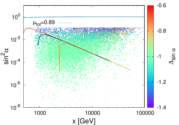
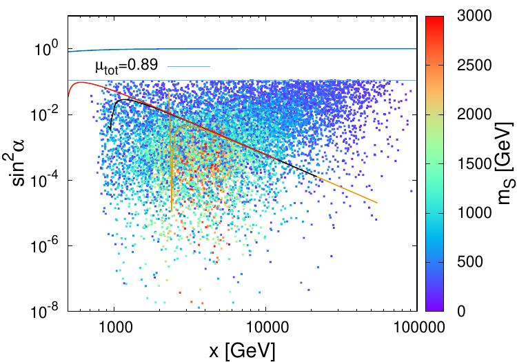
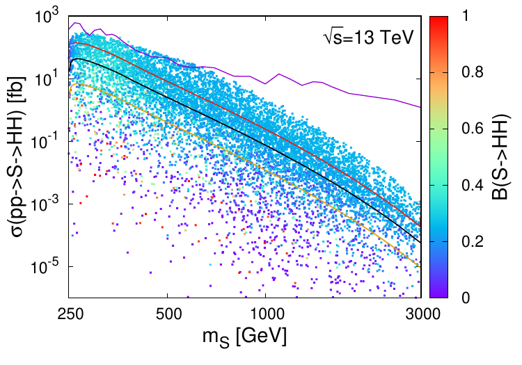
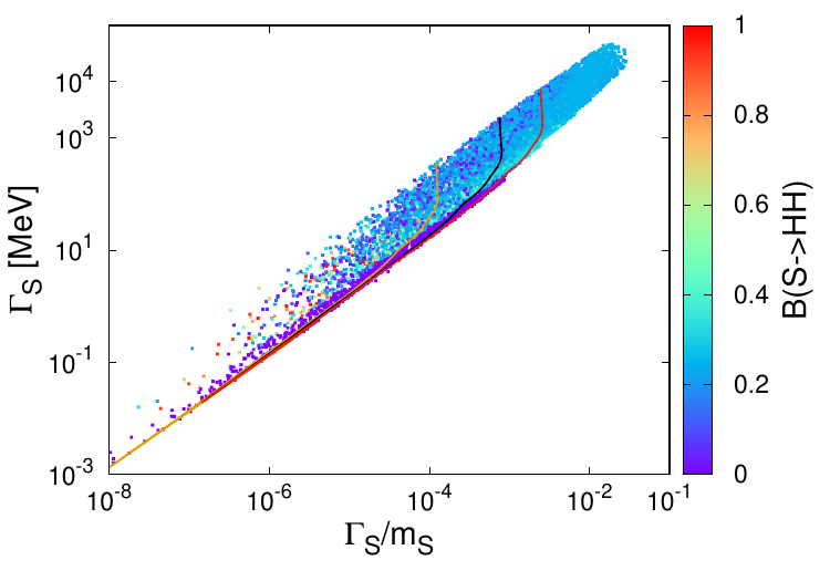
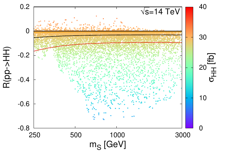
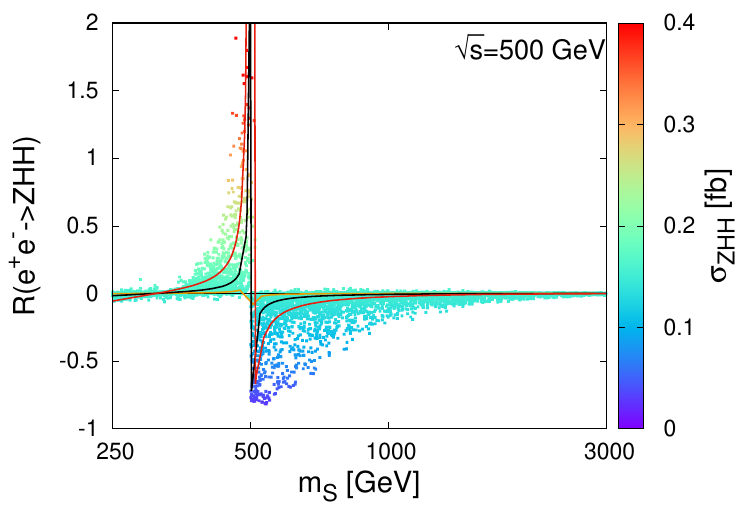
Figure 3: In the upper range, the mixing ($s_{\alpha}^{2}$) versus the singlet VEV $x$, where the palette shows the relative radiative contribution to mixing $\Delta_{\sin\alpha}$ (left) and the heavy scalar mass (middle). The upper blue line corresponds to the tree-level value of the mixing [$(s_{\alpha}^{(0)})^{2}=x^{2}/(\upsilon^{2}+x^{2})$] and $\mu_{tot}=0.89$ represents the experimental bound on the Higgs signal strength in the absence of non-SM Higgs decay modes. The orange, black and purple lines correspond to the toy model with the parameters {$N_{1}=6~{},\alpha_{1}=\beta_{1}=0.2$}, {$N_{2}=12~{},\alpha_{2}=\beta_{2}=0.5$} and {$N_{3}=24~{},\alpha_{3}=\beta_{3}=0.9$}, respectively. In the top-right panel, we show the resonant di-Higgs production cross section via the heavy resonance $S$ at $\sqrt{s}=13~{}\mathrm{TeV}$, compared to the combination of the recent ATLAS measurements ATLAS:2021nps (purple curve). Here, the resonant di-Higgs production cross section estimation was based on the heavy Higgs production cross section values given in HevayHiggs . In the lower range, we show in the left panel the total decay width of the heavy resonance versus the ratio $\Gamma_{S}/m_{S}$, where the palette shows its di-Higgs decay branching ratio. In the middle and right panels, we show the relative enhancement (16) for the processes $pp\rightarrow HH@LHC14$ and $e^{-}e^{+}\rightarrow ZHH@ILC500$, where the palette shows the cross section values in $\mathrm{fb}$.

One has to mention that for the upper panels range in Fig. 3, we used 10K benchmark points (BPs) and considered many theoretical and experimental constraints such as the vacuum stability, perturbativity, perturbative unitarity, electroweak precision tests, the di-photon Higgs decay, the Higgs invisible decay when applicable, the Higgs total decay width measurement ATLAS:2018jym , the implications from negative searches for neutralinos and charginos in supersymmetric models on the inert masses, the bounds on DM nucleon scattering cross section from DD experiments (Xenon 1T Aprile:2017iyp ); and the Higgs signal strength at the LHC $\mu_{{\rm tot}}\geq 0.89$ ATLAS:2016neq . For the lower panels range, we omitted the BPs that are excluded by the negative searches for a heavy resonance in the channels $pp\rightarrow S\rightarrow\tau\tau,\,ZZ,\,WW$ and by the negative searches on the resonant di-Higgs production $pp\rightarrow S\rightarrow HH$ via the different channel $HH\rightarrow b\bar{b}\tau\tau,\,b\bar{b}b\bar{b},\,b\bar{b}\gamma\gamma\,$ as mentioned previously. These constraints exclude only 5.35% of the BPs used in the upper panels in Fig. 3. Indeed, there are other relevant constraints to this model such as neutrinos oscillation data, DM relic density and and the lepton flavor violating processes. These constraints are not considered here since we interested on the parameters and constraints that are relevant to the radiative effects on the Higgs sector.

From Fig. 3, one can learn many conclusions. A PRMH scenario is viable for a large parameters space, where the radiative corrections can give rise to the Higgs mass and simultaneously push the scalar mixing to be in agreement with the total Higgs strength bound ATLAS:2016neq . For instance, for heavy scalar masses below $3~{}\mathrm{TeV}$, the one-loop quartic couplings $\lambda_{h}^{1-\ell}$ and $\omega^{1-\ell}$ are not practically constrained by the perturbativity since they are lying in the ranges $[0.07,2.5]$ and $[-1,2]$, respectively. However, the singlet one-loop quartic coupling $10^{-5}<\lambda_{\phi}^{1-\ell}\leq 4\pi$, together with the previous requirements make the singlet scalar VEV lies in the range $600~{}\mathrm{GeV}<x<100~{}\mathrm{TeV}$. Here, the fact that the heavy scalar is barely constrained by the recent RUN-II measurements of ATLAS with 139 $\mathrm{fb}^{-1}$ ATLAS:2020zms ; ATLAS:2020tlo ; ATLAS:2021nps , and CMS with 137 $\mathrm{fb}^{-1}$ CMS:2021klu , this scenario would be within the reach of the coming analysis.

One has to notice that the total decay width of the heavy scalar is much smaller than its mass for most of the viable parameters space, and therefore the narrow width approximation used to estimate the resonant di-Higgs production cross section is justified. In addition, the cross section of the non-resonant di-Higgs production at the LHC $pp\rightarrow HH@LHC14$ is reduced (by up to 75%) for the majority of the parameters space, while it is enhanced for few BPs by less than 10%. For the Z-associated di-Higgs production at the ILC $e^{-}e^{+}\rightarrow ZHH@ILC500$, the cross section is mainly enhanced for $m_{S}<500~{}\mathrm{GeV}$, and reduced for larger values $m_{S}>0$. In this setup, the enhancement/suppression is maximal around $m_{S}\sim\sqrt{s}=500\,\mathrm{GeV}$, since it is not a numerical mis-estimation of the cross section due to the Breit-Wigner corrected propagators used in (17). In case where the measured Z-associated di-Higgs production is reduced (increased) with respect to the SM by less than 30% (more than 100%), the heavy scalar mass is $m_{S}\gtrsim 500~{}\mathrm{GeV}$ ($m_{S}\lesssim 500~{}\mathrm{GeV}$). For completeness, one has to mention that the BPs in Fig. 3 are in agreement with DM constraints such as the DD bounds and the relic density. Here, we enforced the relic density to be $\Omega_{N_{1}}h^{2}>0.12$ due to the annihilation channels $N_{1}N_{1}\rightarrow VV,HH,HS,SS,f\bar{f}$, where the contribution of the channel $N_{1}N_{1}\rightarrow\ell_{\alpha}\ell_{\beta},\nu_{\alpha}\bar{\nu}_{\beta}$ to the annihilation cross section would relax the relic density to match the measured value Soualah:2021xbn , $\Omega_{DM}h^{2}=0.120\pm 0.001$ Aghanim:2018eyx .

The idea of the Higgs as a PGB in a SI framework has been discussed in Foot:2007as . In addition to the EWSB details discussion, the authors had shown that the light CP-even mass could exceed the Higgs mass bound (then, $m_{H}>114~{}\mathrm{GeV}$). They considered two phenomenologically consistent models to validate this possibility. Although in SI models, it has been shown that the slow-roll inflation can be achieved by adding a extra VEVless singlet real scalar that is coupled non-minimally to the gravity. This real field singlet inflationary model does not suffer from a unitarity breakdown at a scale below or comparable to the inflation scale Khoze:2013uia . Here, the singlet field that is responsible for inflation can be also a viable DM candidate. In a non SI model Aravind:2015xst that is similar to our illustrative example, where fermionic DM has been addressed and the EWSB is assisted by a real scalar singlet, it has been shown that the inflaton could either be the Higgs boson or the singlet scalar, and slow-roll inflation can be realized via a non-minimal coupling to gravity. This tells us that achieving a successful slow-roll inflation within the PRMH scenario deserves an extensive investigation to define the viable parameters space region(s).

VI Conclusion

In this work, we have shown that the PRMH scenario within the scale invariance approach is possible; where we have derived the condition the required conditions to be fulfilled by the masses, couplings and multiplicities of the new fields added to the SM. We have described also the experimental constraints that are coming for the recent ATLAS and CMS measurements on the Higgs properties and the negative searches of heavy resonances. Significant part of the parameters space makes this scenario in a good agreement with the data. We have proven that to avoid the constraints from the total Higgs signal strength modifier ATLAS:2016neq , the radiative corrections that give rise to the Higgs mass must be considered in order to push the singlet-doublet scalar mixing to lie in the experimentally allowed region. This leads to non-negligible values for the triple scalar couplings $\lambda_{HHH}$ and $\lambda_{HHS}$, that are strictly vanishing at tree-level. Thus, the PRMH scenario is very sensible to the resonant di-Higgs production $pp\rightarrow S\rightarrow HH$ ATLAS:2021nps , as well the non-resonant ones $pp\rightarrow HH$ and $e^{-}e^{+}\rightarrow ZHH$. We have considered the SI-scotogenic model Ahriche:2016cio as an illustrative example, where we have checked different experimental constraints and given some predictions about (Z-associated) di-Higgs production at ($ILC500$) $LHC14$. The PRMH scenario looks interesting since many physical observables are all triggered together by the radiative effects, and therefore, other aspects should be investigated within this approach, such as the electroweak phase transition (EWPT) strength, gravitational waves produced during the EWPT in addition to the different collider signatures that are relevant to the triple scalar couplings.

Appendix A Scalar Triple Couplings

The triple scalar couplings $\lambda_{HHH}$ and $\lambda_{HHS}$ can be defined as combination of the third derivative of the scalar potential after the EWSB. For example, the coupling $\lambda_{HDD}$ can be estimated as Ahriche:2013vqa

$$\begin{array}[]{c}\lambda_{HHH}=\left.\left\{c_{\alpha}^{3}V_{h,h,h}^{1-\ell}-3s_{\alpha}c_{\alpha}^{2}V_{h,h,\phi}^{1-\ell}+3s_{\alpha}^{2}c_{\alpha}V_{h,\phi,\phi}^{1-\ell}-s_{\alpha}^{3}V_{\phi,\phi,\phi}^{1-\ell}\right\}\right|_{h=\upsilon,\,\phi=x},\\ \lambda_{HHS}=\left.\left\{c_{\alpha}^{2}s_{\alpha}V_{h,h,h}^{1-\ell}+(c_{\alpha}^{3}-2c_{\alpha}s_{\alpha}^{2})V_{h,h,\phi}^{1-\ell}+(s_{\alpha}^{3}-2c_{\alpha}^{2}s_{\alpha})V_{h,\phi,\phi}^{1-\ell}+c_{\alpha}s_{\alpha}^{2}V_{\phi,\phi,\phi}^{1-\ell}\right\}\right|_{h=\upsilon,\,\phi=x},\end{array}$$ (20)

with $V_{x,y,z}^{1-\ell}\equiv\partial^{3}V^{1-\ell}/\partial x\partial y\partial z$. The reason that these couplings vanish at tree-level (i.e., by considering the tree-level potential and the mixing $s_{\alpha}^{(0)}$); is due to the tree-level vacuum structure of all SI SM extensions, where the EWSB is assisted by the real singlet scalar $\phi$. The one-loop couplings in (20) can be estimated by considering the one-loop effective potential (3) and the tree-level mixing $s_{\alpha}^{(0)}$. However, one can obtain more precise values by doing some re-summation. Here, we will use a resummed estimation of the couplings (20) by taking into account the one-loop effective potential (3) and the one-loop mixing $s_{\alpha}^{(1)}$ instead of the tree-level mixing $s_{\alpha}^{(0)}$. We found that the resummed one-loop values for (20) are significantly different from zero; and they are fully triggered by quantum corrections.

Acknowledgements

This work is funded by the University of Sharjah under the research projects No 21021430100 “Extended Higgs Sectors at Colliders: Constraints & Predictions” and No 21021430107 “Hunting for New Physics at Colliders”.

References

- (1) G. Aad et al. [ATLAS], Phys. Lett. B 716 (2012), 1-29 [arXiv:1207.7214 [hep-ex]]. S. Chatrchyan et al. [CMS], Phys. Lett. B 716 (2012), 30-61 [arXiv:1207.7235 [hep-ex]].
- (2) K. A. Meissner and H. Nicolai, Phys. Lett. B 648 (2007), 312-317 [arXiv:hep-th/0612165 [hep-th]].
- (3) S. R. Coleman and E. J. Weinberg, Phys. Rev. D 7 (1973), 1888-1910.
- (4) L. Alexander-Nunneley and A. Pilaftsis, JHEP 09 (2010), 021 [arXiv:1006.5916 [hep-ph]]. J. S. Lee and A. Pilaftsis, Phys. Rev. D 86 (2012), 035004 [arXiv:1201.4891 [hep-ph]]. C. Englert, J. Jaeckel, V. V. Khoze and M. Spannowsky, JHEP 04 (2013), 060 [arXiv:1301.4224 [hep-ph]]. A. Farzinnia, H. J. He and J. Ren, Phys. Lett. B 727 (2013), 141-150 [arXiv:1308.0295 [hep-ph]]. A. D. Plascencia, JHEP 09 (2015), 026 [arXiv:1507.04996 [hep-ph]].
- (5) R. Foot, A. Kobakhidze, K. L. McDonald and R. R. Volkas, Phys. Rev. D 76 075014 (2007) [arXiv:0706.1829 [hep-ph]]. A. Karam and K. Tamvakis, Phys. Rev. D 92 (2015) no.7, 075010 [arXiv:1508.03031 [hep-ph]]. A. Ahriche, K. L. McDonald and S. Nasri, JHEP 10 (2014), 167 [arXiv:1404.5917 [hep-ph]]. M. Lindner, S. Schmidt and J. Smirnov, JHEP 10 (2014), 177 [arXiv:1405.6204 [hep-ph]]. P. Humbert, M. Lindner and J. Smirnov, JHEP 06 (2015), 035 [arXiv:1503.03066 [hep-ph]]. A. Ahriche, A. Manning, K. L. McDonald and S. Nasri, Phys. Rev. D 94 (2016) no.5, 053005 [arXiv:1604.05995 [hep-ph]].
- (6) A. Ahriche, K. L. McDonald and S. Nasri, JHEP 06 (2016), 182 [arXiv:1604.05569 [hep-ph]].
- (7) B. Bellazzini, C. Csaki, J. Hubisz, J. Serra and J. Terning, Eur. Phys. J. C 73 (2013) no.2, 2333 [arXiv:1209.3299 [hep-ph]].
- (8) R. Foot, A. Kobakhidze and R. R. Volkas, Phys. Lett. B 655 (2007), 156-161 [arXiv:0704.1165 [hep-ph]].
- (9) G. Aad et al. [ATLAS and CMS], JHEP 08 (2016), 045 [arXiv:1606.02266 [hep-ex]].
- (10) G. Aad et al. [ATLAS], Phys. Rev. Lett. 125 (2020) no.5, 051801 [arXiv:2002.12223 [hep-ex]].
- (11) G. Aad et al. [ATLAS], Eur. Phys. J. C 81 (2021) no.4, 332 [arXiv:2009.14791 [hep-ex]].
- (12) A. Tumasyan et al. [CMS], [arXiv:2109.06055 [hep-ex]].
- (13) G. Aad et al. [ATLAS], ATL-PHYS-PUB-2021-031.
- (14) G. Aad et al. [ATLAS], ATLAS-CONF-2021-030.
- (15) G. Aad et al. [ATLAS], ATLAS-CONF-2021-035.
- (16) G. Aad et al. [ATLAS], ATLAS-CONF-2021-016.
- (17) R. Soualah and A. Ahriche, Phys. Rev. D 105 (2022) no.5, 055017 [arXiv:2111.01121 [hep-ph]].
- (18) A. Ahriche, “The scale invariant scotogenec model: RGE & the vacuum structure”, in preparation.
- (19) M. Heikinheimo, A. Racioppi, M. Raidal and C. Spethmann, Phys. Lett. B 726 (2013), 781-785 [arXiv:1307.7146 [hep-ph]]. A. Ahriche, A. Arhrib and S. Nasri, Phys. Lett. B 743 (2015), 279-283 [arXiv:1407.5283 [hep-ph]].
- (20) A. Ahriche, A. Arhrib and S. Nasri, JHEP 02 (2014), 042 [arXiv:1309.5615 [hep-ph]].
- (21) M. Spira, [arXiv:hep-ph/9510347 [hep-ph]].
- (22) J. Alwall, M. Herquet, F. Maltoni, O. Mattelaer and T. Stelzer, JHEP 06 (2011), 128 [arXiv:1106.0522 [hep-ph]].
- (23) N. Baouche, A. Ahriche, G. Faisel and S. Nasri, Phys. Rev. D 104 (2021) no.7, 075022 [arXiv:2105.14387 [hep-ph]].
- (24) S. Kanemura, S. Kiyoura, Y. Okada, E. Senaha and C. P. Yuan, Phys. Lett. B 558, 157-164 (2003) [arXiv:hep-ph/0211308 [hep-ph]]. S. Kanemura, Y. Okada, E. Senaha and C. P. Yuan, Phys. Rev. D 70, 115002 (2004) [arXiv:hep-ph/0408364 [hep-ph]]. V. Khachatryan et al. [CMS], Phys. Rev. D 92 (2015) no.7, 072010 [arXiv:1507.06656 [hep-ex]].
- (25) M. Aaboud et al. [ATLAS], Phys. Lett. B 786 (2018), 223-244 [arXiv:1808.01191 [hep-ex]].
- (26) E. Aprile et al. [XENON Collaboration], Phys. Rev. Lett. 119, no. 18, 181301 (2017) [arXiv:1705.06655 [astro-ph.CO]].
- (27) https://twiki.cern.ch/twiki/bin/view/LHCPhysics/LHCHWG
- (28) N. Aghanim et al. [Planck], Astron. Astrophys. 641, A6 (2020) [arXiv:1807.06209 [astro-ph.CO]].
- (29) V. V. Khoze, JHEP 11 (2013), 215 [arXiv:1308.6338 [hep-ph]].
- (30) A. Aravind, M. Xiao and J. H. Yu, Phys. Rev. D 93 (2016) no.12, 123513 [erratum: Phys. Rev. D 96 (2017) no.6, 069901] [arXiv:1512.09126 [hep-ph]].