Hölder continuity of the Lyapunov exponents of linear cocycles
over hyperbolic maps

Abstract.

Given a hyperbolic homeomorphism on a compact metric space, consider the space of linear cocycles over this base dynamics which are Hölder continuous and whose projective actions are partially hyperbolic dynamical systems. We prove that locally near any typical cocycle, the Lyapunov exponents are Hölder continuous functions relative to the uniform topology. This result is obtained as a consequence of a uniform large deviations type estimate in the space of cocycles. As a byproduct of our approach, we also establish other statistical properties for the iterates of such cocycles, namely a central limit theorem and a large deviations principle.

1. introduction

Let $M$ be a compact metric space with no isolated points and let $f\colon M\to M$ be a hyperbolic homeomorphism. Examples of such systems are Anosov diffeomorphisms on a compact manifold, nontrivial hyperbolic attractors, horseshoes and Markov shifts. Moreover, Bowen [13] showed that every hyperbolic homeomorphism is conjugated, via a Hölder continuous function to a topological Markov shift in a finite number of symbols.

Given any Hölder continuous observable (referred to as a potential) on $M$, there exists an equilibrium state (which is unique, if we also assume the topological transitivity of the system), that is, there is an $f$-invariant Borel probability measure $\mu$ on $M$ which maximizes the pressure. Such measures, which are ergodic, correspond, via the semi-conjugation given by Bowen’s theorem, to measures that admit a local product structure with Hölder continuous density.

A linear cocycle over the base dynamical system $(M,f,\mu)$ is a skew product map

$$F_{A}\colon M\times\mathbb{R}^{d}\to M\times\mathbb{R}^{d},\quad F_{A}(x,v)=\left(f(x),A(x)v\right)\,,$$

where $A\colon M\to\mathrm{GL}(d,\mathbb{R})$ is a Hölder continuous matrix valued function.

The iterates of this new dynamical system are

$$F_{A}^{n}(x,v)=\left(f^{n}(x),A^{n}(x)v\right)\,,$$

where

$$A^{n}(x):=A(f^{n-1}x)\ldots A(f(x))\,A(x)\,.$$

A linear cocycle $F_{A}$ is determined by, and thus can be identified with the matrix valued, Hölder continuous function $A\colon M\to\mathrm{GL}(d,\mathbb{R})$. We endow the space $C^{\alpha}(M,\mathrm{GL}(d,\mathbb{R}))$ of such functions with the uniform distance

$$d(A,B):={\left\lVert A-B\right\rVert}_{\infty}+{\left\lVert A^{-1}-B^{-1}\right\rVert}_{\infty}.$$

By Furstenberg-Kesten’s theorem, we have the following $\mu$-a.e. convergence of the maximal expansion of the iterates of the linear cocycle:

$$\frac{1}{n}\,\log{\left\lVert A^{n}(x)\right\rVert}\to L_{1}(A)\,,$$ (1.1)

where the limit $L_{1}(A)$ is called the maximal Lyapunov exponent of the cocycle $A$.

The other Lyapunov exponents are defined similarly: $L_{2}(A)$ corresponds to the second largest expansion (or singular value) of the iterates of $A$ and so on, until $L_{d}(A)$.

A linear cocycle $F_{A}$ induces the projective cocycle

$$\hat{F}_{A}\colon M\times\mathbb{P}(\mathbb{R}^{d})\to M\times\mathbb{P}(\mathbb{R}^{d}),\quad F_{A}(x,\hat{v})=\left(f(x),\widehat{A(x)v}\right)\,.$$

We will assume that the projective cocycle $\hat{F}_{A}$ is a partially hyperbolic dynamical system, which is an open property and corresponds, via the semi-conjugacy in Bowen’s theorem, to the linear cocycle being fiber bunched (or nearly conformal).

We also assume that the cocycle $A$ is typical in the sense of Bonatti and Viana, which is an open and dense property and ensures the simplicity of the Lyapunov exponents. Precise definitions of this and other relevant concepts will be given in the next section.

The iterates of a linear cocycle are multiplicative processes that generalize products of i.i.d. random matrices, which in turn represent multiplicative analogues of sums of i.i.d. scalar random variables. The study of their statistical properties, that is, of the convergence in (1.1), is an interesting problem in itself, with important consequences elsewhere. Limit theorems (e.g. a large deviations principle and a central limit theorem) were first obtained by E. Le Page [23] for Bernoulli base dynamics and by P. Bougerol [9] for Markov type cocycles. Related results, in the same setting, were more recently established by P. Duarte and S. Klein, see [18] and [17, Chapter 5]).

For the case of linear cocycles over hyperbolic systems, in the same setting of this paper, S. Gouëzel and L. Stoyanov [20] obtained a large deviations principle, while K. Park and M. Piraino [27] obtained a central limit theorem (and a large deviations principle).

We are interested in large deviations type (LDT) estimates that are finitary (non asymptotic), effective and uniform in the cocycle. Such estimates are also called concentration inequalities in probabilities.

Definition 1.1.

Let $A\colon M\to\mathrm{GL}(d,\mathbb{R})$ be a linear cocycle over an ergodic system $(M,f,\mu)$ as above. We say that $A$ satisfies an LDT estimate if there are constants $C=C(A)<\infty$ and $k=k(A)>0$ such that for all  $0<\varepsilon<1$ and $n\in\mathbb{N}$,

$$\mu\left\{x\in M\colon\,\bigl{|}\frac{1}{n}\,\log{\left\lVert A^{n}(x)\right\rVert}-L_{1}(A)\bigr{|}>\varepsilon\,\right\}\leq C\,e^{-{k\,\varepsilon^{2}}\,n}\;.$$

We call such an estimate uniform if it holds for all cocycles in some neighborhood of $A$, with the same constants $C$ and $k$.

The first result of this paper is the following.

Theorem 1.1.

Let $f\colon M\to M$ be a hyperbolic homeomorphism, let $\mu$ be an equilibrium state of a Hölder continuous potential and let $A\colon M\to\mathrm{GL}(d,\mathbb{R})$ be a Hölder continuous linear cocycle. Assume that $A$ is typical and that the corresponding projective cocycle is a partially hyperbolic system. Then $A$ satisfies a uniform large deviations type estimate.

Ou approach is based upon the study of the spectral properties of the Markov (or transition) operator associated to the projective cocycle $\hat{F}_{A}$ and defined on an appropriate space of observables. In other related works, e.g. [27], it is the transfer operator that plays a similar rôle. Our method allows for a more quantitative control of various parameters, thus ensuring the uniformity of the LDT estimate above. Moreover, as a by-product of this approach and using an abstract CLT for stationary Markov processes due to Gordin and Lifšic [19], we establish the following central limit theorem in the setting of Theorem 1.1.

Theorem 1.2.

Given a cocycle $A$ as above, there exists $0<\sigma<\infty$ such that for every $v\in\mathbb{R}^{d}\setminus\{0\}$ and $a\in\mathbb{R}$,

$$\lim_{n\to\infty}\mu\left\{x\in M\colon\frac{\log{\left\lVert A^{n}(x)\,v\right\rVert}-n\,L_{1}(A)}{\sqrt{n}}\leq a\,\right\}=\frac{1}{\sigma\sqrt{2\pi}}\int_{-\infty}^{a}e^{-\frac{t^{2}}{2\sigma^{2}}}dt$$

Note that compared with the main result in [27], the positivity of the variance is an implicit conclusion rather than an additional hypothesis.

Furthermore, we also establish a large deviations principle.

An important question in the theory of linear cocycles is the behavior of the Lyapunov exponents under small perturbations of the data. In particular, the continuity of the maximal Lyapunov exponent is considered a difficult problem in most settings. It has been studied successfully in the case of cocycles over Bernoulli systems by, amongst others, C. Bocker and M. Viana [6], E. Malheiro and M. Viana [25] and by L. Backes, A. Brown and C. Butler [3].

Furthermore, the study of finer continuity properties (e.g. Hölder continuity) of the Lyapunov exponents was initiated by Le Page [24] for the Bernoulli case and further extended to related settings, see for instance P. Duarte and S. Klein [17, 18] and E. Tall and M. Viana [30].

In [17, Chapter 2] it was established a relationship between the availability of uniform LDT estimates in any abstract space of cocycles and the Hölder continuity of the Lyapunov exponents. The main result of our paper is thus the following.

Theorem 1.3.

Let $f\colon M\to M$ be a hyperbolic homeomorphism and let $\mu$ be an equilibrium state of a Hölder continuous potential. Consider the open set of typical Hölder continuous cocycles $A\colon M\to\mathrm{GL}(d,\mathbb{R})$ whose projective actions are partially hyperbolic. Then the Lyapunov exponents are locally Hölder continuous functions of the cocycle.

An important class of examples of linear cocycles are the Schrödinger cocycles, whose iterates represent the transfer matrices used to formally solve a discrete Schrödinger equation. More precisely, let $v\colon M\to\mathbb{R}$ be a potential function and let $\lambda>0$ be a coupling constant. Given a base point $x\in M$, the discrete Schrödinger operator $H_{\lambda}(x)$ acts on $l^{2}(\mathbb{Z})$ as follows: if $\psi=\{\psi_{n}\}_{n\in\mathbb{Z}}\in l^{2}(\mathbb{Z})$, then

$$\big{[}H_{\lambda}(x)\psi\big{]}_{n}:=-(\psi_{n+1}+\psi_{n-1})+\lambda\,v(f^{n}x)\psi_{n}\quad\text{ for all }n\in\mathbb{Z}\,.$$

The associated Schrödinger equation, $H_{\lambda}(x)\psi=E\psi$, where $E\in\mathbb{R}$, is a second order finite differences equation, which is solved recursively by iterating the cocycle

$$S_{E,\lambda}\colon M\to\operatorname{SL}(2,\mathbb{R}),\quad S_{E,\lambda}(x):=\left[\begin{array}[]{ccc}\lambda v(x)-E&&-1\\ 1&&\phantom{-}0\\ \end{array}\right]\,.$$

Assuming that the base dynamics is an Anosov linear toral automorphism, for a smooth potential function $v$ and for small enough coupling constants $\lambda$, V. Chulaevski and T. Spencer [15] proved the positivity of the Lyapunov exponent of the cocycle $(f,S_{E,\lambda})$ for all energies, while J. Bourgain and W. Schlag [12] proved that the corresponding Schrödinger operator satisfies Anderson localization.

In the (more general) setting of this paper we obtain the following.

Theorem 1.4.

Assume that the base dynamics $(M,f,\mu)$ is given by a topologically mixing, uniformly hyperbolic $C^{1}$ diffeomorphism and that $v\colon M\to\mathbb{R}$ is a Hölder continuous potential function with $\int v\,d\mu\neq 0$.

Given $\delta>0$ there exists $\lambda_{0}>0$ such that for all $0<\bigl{|}\lambda\bigr{|}<\lambda_{0}$ and $E\in\mathbb{R}$ with $\bigl{|}E\bigr{|}<2-\delta$, the cocycle $(f,S_{E,\lambda})$ has positive Lyapunov exponent.

Moreover, the maximal Lyapunov exponent is a Hölder continuous function of the parameters $E$ and $\lambda$.

Furthermore, the statistical properties derived above (uniform LDT estimates, CLT) also hold for the iterates of this cocycle.

We remark that positivity and Hölder continuity of the Lyapunov exponents together with uniform LDT estimates for such cocycles are often used as main ingredients in establishing Anderson localization of the corresponding Schrödinger operator (see for instance J. Bourgain and M. Goldstein [11], J. Bourgain and W. Schlag [12], S. Jitomirskaya and X. Zhu [22] or the survey of D. Damanik [16]). This topic, in the setting of this paper, will be considered in a separate project.

We would like to note that, according to an old private conversation between the second author and D. Damanik, the Schrödinger operator with potential defined over similar types of base dynamics as in this paper has also been studied by A. Avila and D. Damanik. We are not aware of the current status of their project, nor of the methods employed, although we expect them to be different from ours.

The paper is organized as follows. In Section 1 we formally define the main concepts used in this paper and provide the precise formulation of the main result, the continuity Theorem 1.3. In Sections 3 and 4 we introduce some technical tools such as the holonomy reduction, the Markov operator (and its quasi-compactness property) and stationary measures. In Sections 5 and 6 we establish the strong mixing of the Markov operator associated to the base dynamics and respectively to the projective fiber dynamics. Based on this, in Section 7 we prove the uniform LDT estimate in Theorem 1.1 and as a consequence of an abstract continuity result, we derive the main Theorem 1.3. Moreover, as explained in Remark 7.1, the argument can be adapted to also obtain a large deviations principle. Furthermore, the strong mixing of the Markov operator corresponding to the fiber dynamics together with an abstract central limit theorem are used in Section 8 to derive Theorem 1.2. Finally, in Section 9 we apply these results to Schrödinger cocycles and establish Theorem 1.4.

2. Main concepts

In this section we formally introduce the concepts mentioned in the introduction and formulate the results which imply Theorem 1.3.

2.1. Base dynamics

Let $M$ be a compact metric space with no isolated points and let $f\colon M\to M$ be a homeomorphism. For a point $x\in M$ and for $\epsilon>0$ small we define the local $\epsilon$-stable and respectively $\epsilon$-unstable sets of $x$ by

$$W^{s}_{\epsilon}\left(x\right) :=\left\{x\colon d\left(f^{k}(y),f^{k}(x)\right)<\epsilon\,\text{ for all }k\geq 0\right\}\text{ and }$$

$$W^{u}_{\epsilon}\left(x\right) :=\left\{x\colon d\left(f^{k}(x),f^{k}(y)\right)<\epsilon\,\text{ for all }k\leq 0\right\}.$$

Following M.Viana [31], we call a homeomorphism $f$ (uniformly) hyperbolic if there are constants $C<\infty$, $\epsilon>0$, $\tau>0$ and $\lambda\in(0,1)$ such that for all $x\in M$ we have

1. $d\left(f^{n}(y_{1}),f^{n}(y_{2})\right)\leq C\,\lambda^{n}d(y_{1},y_{2})$   for all $y_{1},y_{2}\in W^{s}_{\epsilon}(x)$ and $n\geq 0$;

2. $d\left(f^{-n}(y_{1}),f^{-n}(y_{2})\right)\leq C\,\lambda^{n}d(y_{1},y_{2})$   for all $y_{1},y_{2}\in W^{u}_{\epsilon}(x)$ and $n\geq 0$;

3. if $d(x,y)\leq\tau$, then $W^{u}_{\epsilon}(x)$ and $W^{s}_{\epsilon}(y)$ intersect in a unique point, which is denoted by $[x,y]$ and which depends continuously on $(x,y)$.

For this $\epsilon$, the sets $W^{s}_{\mathrm{loc}}(x):=W^{s}_{\epsilon}(x)$ and $W^{u}_{\mathrm{loc}}(x):=W^{u}_{\epsilon}(x)$ are referred to simply as local stable and unstable sets of $f$.

See also J. Ombach [26] for other characterizations of hyperbolicity.

Typical examples of such dynamical systems are Anosov diffeomorphisms, Markov shifts, non trivial hyperbolic attractors and horseshoes.

Recall that given a Hölder continuous potential $\varphi\colon M\to\mathbb{R}$, there is a corresponding equilibrium state measure on $M$, which is unique if $f$ is topologically transitive.

It was essentially established by R. Bowen [13] (see also V. Baladi [4] and the review by V. Alekseev and M. Yakobson [1] for more general settings that include ours) that uniformly hyperbolic homeomorphisms are semi-conjugated to a Markov shift. This means that for every uniformly hyperbolic homeomorphism $f\colon M\to M$ there exists a topological Markov shift $T\colon X\to X$ and a Hölder continuous map $\pi\colon X\to M$ such that $\pi\circ T=f\circ\pi$. Moreover, we can restrict $\pi$ so that it becomes a homeomorphism on a set that has total measure for every $T$-invariant measure $\mu$. Furthermore, we have a one to one correspondence between the equilibrium states of the Markov shift $(X,T)$ and those of $(M,f)$.

Let us then consider a topological Markov shift $(X,T)$, where the phase space $X=\{1,\ldots,\ell\}^{\mathbb{Z}}$, the transformation $T\colon X\to X$ is the left shift homeomorphism $Tx=T\{x_{i}\}_{i\in\mathbb{Z}}:=\{x_{i+1}\}_{i\in\mathbb{Z}}$ and the distance on $X$ is given by

$$d(x,y):=2^{-\min\{i\colon x_{i}\neq y_{i}\text{ or }x_{-i}\neq y_{-i}\}}\,.$$

Assume that $\mu\in\mathrm{Prob}(X)$ is a $T$-invariant measure. Given the symbols $a_{0},\ldots,a_{k}\in\{1,\ldots,\ell\}$ consider the corresponding cylinder

$$[a_{0},\ldots,a_{k}]:=\{x\in X\colon x_{i}=a_{i}\,\text{ for }\,0\leq i\leq k\}.$$

Define $X^{-}:=\{1,\ldots,\ell\}^{-\mathbb{N}\cup\{0\}}$ and $X^{+}:=\{1,\ldots,\ell\}^{\mathbb{N}}$, where $\mathbb{N}:=\{1,2,3,\ldots\}$. Let $T_{+}:X^{+}\to X^{+}$ be the non-invertible left shift and $T_{-}:X^{-}\to X^{-}$ be the non-invertible right shift. Denote by $P_{\pm}\colon X\to X^{\pm}$ the corresponding canonical projections. Given $x\in X$, define the local stable set

$$W^{s}_{\mathrm{loc}}(x):=\{y\in X\colon y_{n}=x_{n}\,\text{ for all }\,n\geq 0\},$$

and the local unstable set

$$W^{u}_{\mathrm{loc}}(x):=\{y\in X\colon y_{n}=x_{n}\,\text{ for all }\,n\leq 0\}.$$

Note that $W^{u}_{\mathrm{loc}}(x)=P_{-}^{-1}(P_{-}(x))$ for all $x\in X$ and likewise $W^{s}_{\mathrm{loc}}(x)=P_{+}^{-1}(P_{+}(x))\cap[x_{0}]$ for all $x\in X$. Hence

$$W^{u}_{\mathrm{loc}}(x)=W^{u}_{\mathrm{loc}}(y)\quad\Leftrightarrow\quad P_{-}(x)=P_{-}(y).$$

$$W^{s}_{\mathrm{loc}}(x)=W^{s}_{\mathrm{loc}}(y)\quad\Leftrightarrow\quad x_{0}=y_{0}\,\text{ and }\,P_{+}(x)=P_{+}(y).$$

Therefore, locally inside a cylinder $[i]$ of size $1$, we can make the identifications

$$[i]\cap X^{-} \equiv X/W^{u}_{\mathrm{loc}}\equiv W^{s}_{\mathrm{loc}}(q)$$

$$X^{+} \equiv X/W^{s}_{\mathrm{loc}}\equiv W^{u}_{\mathrm{loc}}(q)$$

where the right-hand sides represent the local stable and unstable sets of a reference point $q\in[i]$.

Denote by $\mu_{[i]}$ the restriction of the measure $\mu$ to the cylinder $[i]$. Define $\mu^{+}_{i}:=(P_{+})_{\ast}\mu_{[i]}$, which is a measure on $X^{+}=W^{u}_{\mathrm{loc}}(q)$ and $\mu^{-}_{i}:=(P_{-})_{\ast}\mu_{[i]}$, which is a measure on $[i]\cap X^{-}=W^{s}_{\mathrm{loc}}(q)$. Consider the lipeomorphism (by-Lipschitz homeomorphism)

$$h\colon[i]\to W^{s}_{\mathrm{loc}}(q)\times W^{u}_{\mathrm{loc}}(q)\equiv[i]\cap X^{-}\times X^{+}$$

defined by $h(x):=(P_{-}(x),P_{+}(x))$.

Definition 2.1.

We say that $\mu$ has local product structure with Hölder density if there exists $\rho:X^{-}\times X^{+}\to(0,+\infty)$ a Hölder continuous function such that for each $i\in\{1,\ldots,\ell\}$,   $h_{\ast}\mu_{[i]}=\rho|_{[i]}\,(\mu^{-}_{i}\times\mu^{+}_{i})$.

Remark 2.1.

By redefining the symbols, we note that it is sufficient for the product structure to occur at a smaller scale, corresponding to cylinders with length $>1$.

As explained below, examples of such measures are the equilibrium states of Hölder continuous potentials.

Let $\mu$ be a $T$-invariant measure on $X$. Then $\mu^{+}:=(P_{+})_{*}\mu$ is a $T_{+}$-invariant measure on $X^{+}$. Let $J_{\mu^{+}}T_{+}$ be the Jacobian of $T_{+}$.

Theorem 2.1.

If $J_{\mu^{+}}T_{+}>0$ and it is Hölder continuous, then $\mu$ has local product structure with Hölder continuous density.

Proof.

Given $x^{+}$ and $y^{+}$ in the same cylinder, define $h_{x^{+},y^{+}}\colon P_{+}^{-1}(x^{+})\to P_{+}^{-1}(y^{+})$ by $h_{x^{+},y^{+}}(x)=y$, where $y_{n}=y^{+}_{n}$ for $n>0$ and $y_{n}=x_{n}$ for $n\leq 0$.

Using Rokhlin’s disintegration theorem, there exists a disintegration $x^{+}\mapsto\mu^{s}_{x^{+}}$ of $\mu$ relative to the partition $\{P_{+}^{-1}(x^{+}),x^{+}\in X^{+}\}$. By [8, Lemma 2.6], the measure $(h_{x^{+},y^{+}})_{*}\mu^{s}_{x^{+}}$ is absolutely continuous with respect to $\mu^{s}_{y^{+}}$. Moreover by [8, Lemma 2.4] the corresponding Jacobian $Jh_{x^{+},y^{+}}$, where $(h_{x^{+},y^{+}})_{*}\mu^{s}_{x^{+}}=Jh_{x^{+},y^{+}}\,\mu^{s}_{y^{+}}$, is given by

$$Jh_{x^{+},y^{+}}(x)=\lim_{n\to\infty}\frac{J_{\mu^{+}}T_{+}(x_{n})}{J_{\mu^{+}}T_{+}(y_{n})}\,,$$

where $x_{n}=P^{+}(T^{-n}(x))$.

Given a cylinder $[i]$, fix $x^{+}\in[i]$, we can write $\mu_{i}=\rho\,\mu^{s}_{x^{+}}\times\mu^{+}$ with $\rho(y^{+},z^{-})=Jh_{x^{+},y^{+}}(z)$, where $z_{n}=y^{+}_{n}$ if $n>0$ and $z_{n}=z^{-}_{n}$ if $n\leq 0$. So we are left to prove that $Jh_{x^{+},y^{+}}(x)$ is Hölder continuous.

To see this observe that $Jh_{x^{+},y^{+}}(x)=\lim_{n\to\infty}\frac{J_{\mu^{+}}T_{+}(x_{n})}{J_{\mu^{+}}T_{+}(y_{n})}$, then we can see $Jh$ as the holonomy of the linear cocycle $J_{\mu^{+}}T_{+}(x^{+})$ taking values on $\mathbb{R}$, then by Theorem 3.1 below, $Jh_{x^{+},y^{+}}$ varies Hölder continuously with respect to $(x^{+},y^{+})$. ∎

Remark 2.2.

The above result shows that measures with Hölder continuous Jacobian for the one sided shift $T^{+}$ have local product structure. An equilibrium state for $T$ is the lift of an equilibrium state for $T^{+}$ and they have Hölder continuous Jacobian if the potential is Hölder continuous, see [13]. So equilibrium states of Hölder continuous potentials satisfy our hypothesis.

2.2. Fiber dynamics

Let $A\colon X\to\mathrm{GL}(d,\mathbb{R})$ be a linear cocycle over the shift $T$. Given $\beta>0$ we say that $A$ admits $\beta$-Hölder stable holonomies if there exist $C<\infty$ and a family of linear maps $\left\{H^{s}_{x,y}\in\mathrm{GL}(d,\mathbb{R})\colon x\in X,y\in W^{s}_{\mathrm{loc}}(x)\right\}$ with the following properties:

1. $H^{s}_{x,x}=\operatorname{id}$ and $H^{s}_{x,y}\circ H^{s}_{y,z}=H^{s}_{x,z}$ for $x\in X$, $y,z\in W^{s}_{\mathrm{loc}}(x)$,

2. $A(y)\circ H^{s}_{x,y}=H^{s}_{T(x),T(y)}\circ A(x)$ for $x\in X$, $y\in W^{s}_{\mathrm{loc}}(x)$,

3. ${\left\lVert H^{s}_{x,y}-\operatorname{id}\right\rVert}\leq C\operatorname{dist}(x,y)^{\beta}$,

4. ${\left\lVert H^{s}_{x,y}-H^{s}_{x^{\prime},y^{\prime}}\right\rVert}\leq C\left(d(x,x^{\prime})^{\beta}+d(y,y^{\prime})^{\beta}\right)$ for $y\in W^{s}_{\mathrm{loc}}(x)$ and $y^{\prime}\in W^{s}_{\mathrm{loc}}(x^{\prime})$.

Moreover, we say that $A$ admits $\beta$-Hölder unstable holonomies if the inverse cocycle admits $\beta$-Hölder stable holonomies.

We say that an $\alpha$-Hölder linear cocycle $A:X\to\mathrm{GL}(d,\mathbb{R})$ is fiber bunched if there exists $N\in\mathbb{N}$, such that

$${\left\lVert A^{N}(x)\right\rVert}{\left\lVert A^{N}(x)^{-1}\right\rVert}2^{-N\alpha}<1\quad\text{ for all }\ x\in X.$$

Note that a cocycle is fiber bunched if and only if the corresponding projective cocycle is a partially hyperbolic dynamical system.

If $A$ is fiber bunched then there exists $\beta>0$ such that $A$ admits $\beta$-Hölder stable and unstable holonomies (see Theorem 3.1) and $\beta$ can be taken uniformly in a $C^{0}$ neighborhood of $A$. Moreover, for every $*=s$ or $u$, $x\in X$, $y\in W^{*}_{\mathrm{loc}}(x)$, the map $A\mapsto H^{*,A}_{x,y}$ varies continuously in the uniform topology.

From now on we fix the base dynamics $T\colon X\to X$ with an ergodic measure $\mu$ that has local product structure with Hölder density and we consider the space of $\alpha$-Hölder linear cocycles over this dynamics. We endow this space with the Hölder norm

$${\left\lVert A\right\rVert}_{\alpha}=\sup_{x\in X}{\left\lVert A(x)\right\rVert}+\sup_{x\neq y}\frac{{\left\lVert A(x)-A(y)\right\rVert}}{{\left\lVert x-y\right\rVert}^{\alpha}}.$$

We recall the following definition from [8].

Definition 2.2.

We say that a cocycle $A\colon X\to\mathrm{GL}(d,\mathbb{R})$ satisfies the pinching and twisting conditions if there exists a $q$-periodic point $a=T^{q}(a)$ and an associated homoclinic point $z\in W^{u}_{\mathrm{loc}}(a)$ with $z^{\prime}=T^{l}z\in W^{s}_{\mathrm{loc}}(a)$, for some $l\in\mathbb{N}$, both $a$ and $z\in\operatorname{supp}(\mu)$, such that the transition map $\psi_{a,z,z^{\prime}}:\mathbb{R}^{d}\to\mathbb{R}^{d}$, defined by $\psi_{a,z,z^{\prime}}:=H^{s}_{z^{\prime},a}\,A^{l}(z)\,H^{u}_{a,z}$, satisfies:

1. The eigenvalues of the matrix $A^{q}(a)$ have multiplicity one and different absolute values. Consider (for the next clause) the corresponding eigenvectors $e_{1},\ldots,e_{d}$ of $A^{q}(a)$.

2. $\mathrm{span}\{\psi_{a,z,z^{\prime}}^{\pm 1}(e_{i})\colon i\in I\}+\mathrm{span}\{e_{j}\colon j\in J\}=\mathbb{R}^{d}$ for any $I,J\subset\{1,\dots,n\}$ such that $\#I+\#J=n$.

Let $g$ be the matrix of $\psi_{a,z,z^{\prime}}$ written in the base of eigenvectors of $A^{q}(a)$; the twisting condition is then equivalent to all the algebraic minors of $g$ being different from zero.

A cocycle satisfying the pinching and twisting properties is also called $1$-typical.

2.3. Continuity of the Lyapunov exponents

We can now present the precise formulation of the main result of this paper.

Theorem 2.2.

Let $T\colon X\to X$ be the left shift, let $\mu$ be an ergodic measure that has local product structure with Hölder density and let $A\colon X\to\mathrm{GL}(d,\mathbb{R})$ be an $\alpha$-Hölder fiber bunched linear cocycle. If $A$ is $1$-typical then there exists a $C^{0}$ neighborhood of $A$ such that in this neighborhood, the maximal Lyapunov exponent is a Hölder continuous function of the cocycle.

Given a linear cocycle $A\colon X\to\mathrm{GL}(d,\mathbb{R})$ and an integer $1\leq k\leq d$, let $\wedge^{k}A$ be the induced $k$-th exterior power of $A$, where for every base point $x\in X$, $\wedge^{k}A(x)$ acts linearly on $\wedge^{k}\mathbb{R}^{d}$, the $k$-th exterior power of the Euclidean space $\mathbb{R}^{d}$.

Note that the pinching condition on the $k$-th exterior power is equivalent to all the product of $k$ distinct eigenvalues being different, and the twisting condition is equivalent to the action of $g$ on the exterior power having all its algebraic minors different from zero. Both of these conditions are open and dense in the subset of $\alpha$-Hölder fiber bunched cocycles (see [8]).

A linear cocycle is called typical if the pinching and twisting conditions hold for all of its exterior powers.

Note that the maximal Lyapunov exponent of $\wedge^{k}A$ is the sum of the first $k$ Lyapunov exponents of $A$. We then have the following result.

Theorem 2.3.

Let $T\colon X\to X$ be the left shift, let $\mu$ be an ergodic measure that has local product structure with Hölder density and let $A\colon X\to\mathrm{GL}(d,\mathbb{R})$ be an $\alpha$-Hölder continuous fiber bunched linear cocycle. If $A$ is typical then there exists a $C^{0}$ neighborhood of $A$ such that on this neighborhood, all Lyapunov exponents are Hölder continuous functions of the cocycle.

Remark 2.3.

Let $(M,f)$ be a hyperbolic homeomorphism. Given a Hölder continuous linear cocycle $A\colon M\to\mathrm{GL}(d,\mathbb{R})$ we use the Hölder continuous semi-conjugation $\pi$ of $(M,f)$ to a Markov shift $(X,T)$ to obtain the cocycle $A\circ\pi\colon X\to\mathrm{GL}(d,\mathbb{R})$ over the shift $T$. This allows us to transfer the results above to cocycles over uniformly hyperbolic homeomorphisms.

3. Holonomy Reduction

In this section we prove the existence of Hölder holonomies. Moreover we show that up to a conjugacy, the cocycle $A$ can be taken to be constant on unstable sets.

Firstly observe that if $A$ is fiber bunched then there exists $\tau<1$ such that ${\left\lVert A^{N}(x)\right\rVert}{\left\lVert A^{N}(x)^{-1}\right\rVert}2^{-N\alpha}<\tau<1$.

Theorem 3.1.

If $A$ is an $\alpha$-Hölder, fiber bunched cocycle, then there exists $0<\beta<\alpha$ such that $A$ admits $\beta$-Hölder stable holonomies. Moreover, $\beta$ depends on ${\left\lVert A\right\rVert},\alpha,\tau,Lip(T)$, so can be taken uniform on a $C^{0}$ neighborhood of $A$.

Proof.

For $x\in W^{s}_{\mathrm{loc}}(y)$ define $H^{n}_{x,y}={A^{n}(y)}^{-1}A^{n}(x)$ by [7, Lemme 1.12] when $n$ goes to infinity $H^{n}_{x,y}$ converges to a linear map $H^{s}_{x,y}$ that satisfies the first 3 properties on the definition of holonomies, so to prove that is a $\beta$-Hölder holonomy we are left to prove that it also satisfies the $4^{rth}$ property.

Take $x\in W^{s}_{\mathrm{loc}}(y)$ and $x^{\prime}\in W^{s}_{\mathrm{loc}}(y^{\prime})$. By [7, Remarque 1.13] there exists $C_{1}>0$ such that ${\left\lVert H^{s}_{x,y}-H^{n}_{x,y}\right\rVert}\leq C_{1}\tau^{n}d(x,y)^{\alpha}$, so we get that for every $n>0$

$${\left\lVert H^{s}_{x,y}-H^{s}_{x^{\prime},y^{\prime}}\right\rVert}\leq{\left\lVert H^{n}_{x,y}-H^{n}_{x^{\prime},y^{\prime}}\right\rVert}+2C_{1}\tau^{n}.$$ (3.1)

Now observe that

$${\left\lVert H^{n}_{x,y}-H^{n}_{x^{\prime},y^{\prime}}\right\rVert}\leq{\left\lVert{(A^{n})^{-1}}\right\rVert}{\left\lVert A^{n}(x)-A^{n}(x^{\prime})\right\rVert}+{\left\lVert A^{n}\right\rVert}{\left\lVert A^{n}(y)^{-1}-A^{n}(y^{\prime})^{-1}\right\rVert},$$

and let $L=\mathrm{Lip}(T)$, we can estimate

$${\left\lVert A^{n}(x)-A^{n}(x^{\prime})\right\rVert} \leq{\left\lVert A\right\rVert}^{n-1}\sum_{j=0}^{n-1}{\left\lVert A(T^{j}(x))-A(T^{j}(x^{\prime}))\right\rVert}$$

$$\leq{\left\lVert A\right\rVert}^{n-1}(\sum_{j=0}^{n-1}L^{\alpha j})v_{\alpha}(A)\operatorname{dist}(x,x^{\prime})^{\alpha}$$

$$\leq{\left\lVert A\right\rVert}^{n-1}\frac{L^{(n+1)\alpha}}{L^{\alpha}-1}v_{\alpha}(A)\operatorname{dist}(x,x^{\prime})^{\alpha}.$$

Let $K=\max\{{\left\lVert A\right\rVert},{\left\lVert A^{-1}\right\rVert}\}^{2}L^{\alpha}$ and

$$c=2\max\{v_{\alpha}(A),v_{\alpha}(A^{-1})\}\,\frac{L^{\alpha}}{L^{\alpha}-1},$$

then we get ${\left\lVert(A^{n})^{-1}\right\rVert}{\left\lVert A^{n}(x)-A^{n}(x^{\prime})\right\rVert}\leq cK^{n}\operatorname{dist}(x,x^{\prime})^{\alpha}$. We have an analogous inequality for ${\left\lVert A^{n}(y)^{-1}-A^{n}(y^{\prime})^{-1}\right\rVert}$, so from (3.1) we get

$${\left\lVert H^{s}_{x,y}-H^{s}_{x^{\prime},y^{\prime}}\right\rVert}\leq 2cK^{n}\max\{\operatorname{dist}(x,x^{\prime})^{\alpha},\operatorname{dist}(y,y^{\prime})^{\alpha}\}+2C_{1}\tau^{n}.$$ (3.2)

Without loose of generality assume that $\operatorname{dist}(y,y^{\prime})\leq\operatorname{dist}(x,x^{\prime})$. Take any $\gamma<\alpha$ and $n$ such that

$$\frac{\gamma-\alpha}{\log K}\log\operatorname{dist}(x,x^{\prime})-1<n\leq\frac{\gamma-\alpha}{\log K}\log\operatorname{dist}(x,x^{\prime}).$$

We get that

$$cK^{n}\operatorname{dist}(x,x^{\prime})^{\alpha}+C_{1}\tau^{n} \leq c\operatorname{dist}(x,x^{\prime})^{\gamma}+C_{1}\tau^{\frac{\gamma-\alpha}{\log K}\log\operatorname{dist}(x,x^{\prime})-1}$$

$$=c\operatorname{dist}(x,x^{\prime})^{\gamma}+C_{1}e^{-1}\operatorname{dist}(x,x^{\prime})^{\frac{\gamma-\alpha}{\log K}\log\tau},$$

taking $\beta=\min\{\gamma,\frac{\gamma-\alpha}{\log K}\log\tau\}$ we have

$$cK^{n}\operatorname{dist}(x,x^{\prime})^{\alpha}+C_{1}\tau^{n}<(c+e^{-1}C_{1})\operatorname{dist}(x,x^{\prime})^{\beta}.$$

So we can conclude that

$${\left\lVert H^{s}_{x,y}-H^{s}_{x^{\prime},y^{\prime}}\right\rVert}\leq 2(c+C_{1}e^{-1})\max\{\operatorname{dist}(x,x^{\prime})^{\beta},\operatorname{dist}(y,y^{\prime})^{\beta}\}$$ (3.3)

∎

Now we are going to replace $A$ by a cocycle conjugate to $A$ that only depends on the negative part of the sequence, this construction was already made on [2], we explain it here for completeness.

Proposition 3.1.

Given $A:X\to\mathrm{GL}(d,\mathbb{R})$, $\alpha$-Hölder continuous and fiber bunched, there exists $A^{-}:X^{-}\to\mathrm{GL}(d,\mathbb{R})$ $\beta$-Hölder continuous, where $0<\beta<\alpha$ depends on $\alpha$, ${\left\lVert A\right\rVert}$ and $\tau$, such that $A^{s}=A^{-}\circ P^{-}$ is conjugated to $A\circ T^{-1}$. Moreover the conjugation is given by $(x,v)\mapsto(x,H(x)v)$, where $H:X\to\mathrm{GL}(d,\mathbb{R})$ is $\beta$-Hölder continuous, ${\left\lVert H\right\rVert}$ and ${\left\lVert H^{-1}\right\rVert}$ are uniformly bounded on a neighborhood of $A$ and the map $A\mapsto A^{s}$ is continuous on the uniform topology.

Proof.

For each $i\in\Sigma$ fix $p_{i}\in[i]$ and define $\theta:X\to X$ as $\theta(x)$ to be the unique point that belongs to $W^{s}_{\mathrm{loc}}(p_{i})\cap W^{u}_{\mathrm{loc}}(x)$ for $x\in[i]$. Using the unstable holonomies define $A^{s}:X\to\mathrm{GL}(d,\mathbb{R})$ as

$$A^{s}(x)=H^{u}_{x,\theta(x)}A(T^{-1}x)H^{u}_{\theta(T^{-1}x),T^{-1}x}=H^{u}_{T(\theta(T^{-1}x)),\theta(x)}A(T^{-1}\theta(x)),$$

then we have that $A^{s}(x)$ only depend on the negative part of $x$ so there exists $A^{-}:X^{-}\to\mathrm{GL}(d,\mathbb{R})$ such that $A^{s}=A^{-}\circ P^{-}$. Also $A^{s}$ is conjugated to $A\circ T^{-1}$ by the function $(x,v)\mapsto(x,H^{u}_{\theta(T^{-1}x),T^{-1}x}v)$, so $A^{-}$ has the same exponents as $A$. Also fixing $x,y$ the map $A\mapsto H^{u}_{x,y}$ is continuous on the uniform topology, then $A\mapsto A^{s}$ also is.

By theorem 3.1 we have that $A^{-}$ is $\beta$-Hölder. ∎

From now on we assume that $A$ is of the form $A^{-}\circ P^{-}$.

4. Quasi-compact Markov operators

In this section we recall concepts like Markov operators, stationary measures and provide a sufficient criterion for the strong mixing property based on the quasi-compactness of the Markov operator and the classical theorem of Ionescu-Tulcea and Marinescu.

Definition 4.1.

A stochastic dynamical system (SDS) on a compact metric space $\Gamma$ is any continuous mapping $K:\Gamma\to\mathrm{Prob}(\Gamma)$, where the space $\mathrm{Prob}(\Gamma)$ of Borel probability measures on $\Gamma$ is endowed with the weak-$\ast$ topology.

A SDS $K:\Gamma\to\mathrm{Prob}(\Gamma)$ can be recursively iterated as follows

$$K^{n}:\Gamma\to\mathrm{Prob}(\Gamma),\quad K^{n}_{x}:=\int_{\Gamma}K^{n-1}_{y}\,dK_{x}(y)\quad\text{ for }\,n\geq 1,\;x\in\Gamma.$$

Proposition 4.1.

Given a SDS $K:\Gamma\to\mathrm{Prob}(\Gamma)$, the linear operator $\mathcal{Q}_{K}:C^{0}(\Gamma)\to C^{0}(\Gamma)$ defined by $(\mathcal{Q}_{K}\varphi)(x):=\int_{\Gamma}\varphi\,dK_{x}$, is positive, bounded (with norm $\leq 1$) and fixes the constant functions. Its adjoint $\mathcal{Q}^{\ast}$ leaves the convex set $\mathrm{Prob}(\Gamma)$ invariant where $\mathcal{Q}^{\ast}\mu=\int K_{x}\,d\mu(x)$.

Proof.

Straightforward. ∎

Definition 4.2.

$\mathcal{Q}_{K}$ is called the Markov operator of $K$. We call $K$-stationary measure any measure $\mu\in\mathrm{Prob}(\Gamma)$ such that $\mathcal{Q}^{\ast}\mu=\mu$.

The dynamics of the SDS is encapsulated by the operator $\mathcal{Q}_{K}$. We have for instance that $\mathcal{Q}_{K^{n}}=(\mathcal{Q}_{K})^{n}$ for all $n\in\mathbb{N}$.

Theorem 4.1 (Ionescu-Tulcea, Marinescu).

Let $(\mathcal{E}_{1},{\left\lVert\cdot\right\rVert}_{1})$ and $(\mathcal{E},{\left\lVert\cdot\right\rVert})$ be complex Banach spaces, $\mathcal{E}_{1}\subseteq\mathcal{E}$, and $\mathcal{Q}:\mathcal{E}\to\mathcal{E}$ a linear operator such that:

1. $\mathcal{Q}:\mathcal{E}\to\mathcal{E}$ is a bounded operator in $(\mathcal{E},{\left\lVert\cdot\right\rVert})$ with ${\left\lVert\mathcal{Q}\right\rVert}\leq 1$.

2. If $\varphi_{n}\in\mathcal{E}_{1}$, $\varphi\in\mathcal{E}$, $\lim_{n\to\infty}{\left\lVert\varphi_{n}-\varphi\right\rVert}=0$ and ${\left\lVert\varphi_{n}\right\rVert}_{1}\leq C$ for all $n\in\mathbb{N}$ then $\varphi\in\mathcal{E}_{1}$ and ${\left\lVert\varphi\right\rVert}_{1}\leq C$.

3. The inclusion $i:\mathcal{E}_{1}\to\mathcal{E}$ is bounded and compact, i.e., for some constant $M<\infty$, ${\left\lVert\varphi\right\rVert}\leq M\,{\left\lVert\varphi\right\rVert}_{1}$ for all $\varphi\in\mathcal{E}_{1}$ and any bounded set in $(\mathcal{E}_{1},{\left\lVert\cdot\right\rVert}_{1})$ is relatively compact in $(\mathcal{E},{\left\lVert\cdot\right\rVert})$.

4. There exist $0<\sigma<1$, $n_{0}\in\mathbb{N}$ and $C<\infty$ such that for all $\varphi\in\mathcal{E}_{1}$,  ${\left\lVert\mathcal{Q}^{n_{0}}\varphi\right\rVert}_{1}\leq\sigma^{n_{0}}\,{\left\lVert\varphi\right\rVert}_{1}+C\,{\left\lVert\varphi\right\rVert}$.

Then $\mathcal{Q}$ has a finite set $G$ of eigenvalues with finite multiplicity of absolute value $1$ and the rest of the spectrum of $\mathcal{Q}$ is a compact subset of the unit disk $\{z\in\mathbb{C}\colon\bigl{|}z\bigr{|}<1\}$. Furthermore there exist bounded linear operators $\{L_{\lambda}:\mathcal{E}_{1}\to\mathcal{E}_{1}\}_{\lambda\in G}$ and $N:\mathcal{E}_{1}\to\mathcal{E}_{1}$ such that

$$\mathcal{Q}^{n_{0}}=\sum_{\lambda\in G}\lambda^{n_{0}}\,L_{\lambda}+N$$

and for all $\lambda\in G$:

1. $L_{\lambda}\circ L_{\lambda^{\prime}}=0$, for $\lambda^{\prime}\in G$ with $\lambda\neq\lambda^{\prime}$,

2. $L_{\lambda}\circ L_{\lambda}=L_{\lambda}$,

3. $L_{\lambda}\circ N=N\circ L_{\lambda}=0$,

4. $L_{\lambda}(\mathcal{E}_{1})=\{\varphi\in\mathcal{E}_{1}:\mathcal{Q}\varphi=\lambda\,\varphi\}$,

5. $N$ has spectral radius $<1$.

Proof.

See [14, Theorem 7.1.1] or  [21].

∎

Remark 4.1.

The conclusion of Theorem 4.1 is usually expressed saying that $\mathcal{Q}$ is a quasi-compact operator.

Let $(\Sigma,d)$ be a compact metric space with diameter $\leq 1$. Given $0<\alpha\leq 1$ define the seminorm $v_{\alpha}:C^{0}(\Sigma)\to[0,+\infty]$

$$v_{\alpha}(\varphi):=\sup_{x\neq y}\frac{\bigl{|}\varphi(x)-\varphi(y)\bigr{|}}{d(x,y)^{\alpha}}$$

and the norm  ${\left\lVert\varphi\right\rVert}_{\alpha}:=v_{\alpha}(\varphi)+{\left\lVert\varphi\right\rVert}_{\infty}$. The space $(C^{\alpha}(\Sigma),{\left\lVert\cdot\right\rVert}_{\alpha})$ of $\alpha$-Hölder continuous observables $\varphi:\Sigma\to\mathbb{R}$ is a Banach algebra and vector lattice.

The SDS $K$ determines the point-set map

$$\Omega_{K}:\Sigma\to 2^{\Sigma},\quad\Omega_{K}(x):=\overline{\cup_{n\geq 0}\operatorname{supp}(K_{x}^{n})}.$$ (4.1)

Theorem 4.2.

Given $\Sigma$ compact, $\mu\in\mathrm{Prob}(\Sigma)$ and $K:\Sigma\to\mathrm{Prob}(\Sigma)$ a SDS with Markov operator $\mathcal{Q}$, if

1. $\mu$ is a $K$-stationary measure;

2. For every $p\in\mathbb{N}$ and $x\in\Sigma$, $\operatorname{supp}(\mu)\subseteq\Omega_{K^{p}}(x)$;

3. There are constants $0<\alpha\leq 1$, $n_{0}\geq 1$, $C<\infty$ and $0<\sigma<1$ such that for every $\varphi\in C^{\alpha}(\Sigma)$,

   $$v_{\alpha}(\mathcal{Q}^{n_{0}}\varphi)\leq\sigma^{n_{0}}v_{\alpha}(\varphi)+C\,{\left\lVert\varphi\right\rVert}_{\infty}$$

then $\mathcal{Q}$ is strongly mixing on the space $C^{\alpha}(\Sigma)$, i.e., there exists $0<\sigma_{0}<1$ such that for all $\varphi\in C^{\alpha}(\Sigma)$ and some $C_{0}=C_{0}({\left\lVert\varphi\right\rVert}_{\alpha})<\infty$,

$${\left\lVert\mathcal{Q}^{n}\varphi-\smallint\varphi\,d\mu\right\rVert}_{\infty}\leq C_{0}\,\sigma_{0}^{n}\qquad\forall\,n\in\mathbb{N}.$$

Proof.

Consider $(\mathcal{E},{\left\lVert\cdot\right\rVert})=(C^{0}(\Sigma),{\left\lVert\cdot\right\rVert}_{\infty})$ and $(\mathcal{E}_{1},{\left\lVert\cdot\right\rVert}_{1})=(C^{\alpha}(\Sigma),{\left\lVert\cdot\right\rVert}_{\alpha})$. Then the Markov operator $\mathcal{Q}:C^{0}(\Sigma)\to C^{0}(\Sigma)$ satisfies the hypothesis of Theorem 4.1 and, therefore, it is a quasi-compact operator.

Notice that assumption (1) of Theorem 4.1 holds because

$$\bigl{|}(\mathcal{Q}\varphi)(x)\bigr{|}\leq\int\bigl{|}\varphi(y)\bigr{|}\,dK_{x}(y)\leq{\left\lVert\varphi\right\rVert}_{\infty}.$$

If $\varphi_{n}\in C^{\alpha}(\Sigma)$, $\varphi\in C^{0}(\Sigma)$, $\lim_{n\to\infty}{\left\lVert\varphi_{n}-\varphi\right\rVert}_{\infty}=0$ and ${\left\lVert\varphi_{n}\right\rVert}_{\alpha}\leq C$ for all $n\in\mathbb{N}$ then taking the limit of the following inequalities

$$\frac{\bigl{|}\varphi_{n}(x)-\varphi_{n}(y)\bigr{|}}{d(x,y)^{\alpha}}\leq C$$

we get that ${\left\lVert\varphi\right\rVert}_{\alpha}\leq C$. In particular $\varphi$ is $\alpha$-Hölder continuous. This proves assumption (2) of Theorem 4.1. The inclusion $i:C^{\alpha}(\Sigma)\to C^{0}(\Sigma)$ is a bounded linear operator because ${\left\lVert\varphi\right\rVert}_{\infty}\leq{\left\lVert\varphi\right\rVert}_{\alpha}$. It is a compact operator by Ascoli-Arzelá’s Theorem. Therefore, assumption (3) of Theorem 4.1 holds. Finally the assumption (4) of Theorem 4.1 matches hypothesis (3) above.

Lemma 4.2.

Given $\varphi\in C^{0}(\Sigma)$, if $\varphi$ is real valued and $\varphi\leq\mathcal{Q}^{p}\varphi$, for some $p\geq 1$, then $\varphi=c$ is constant on $\operatorname{supp}(\mu)$ with $\varphi\leq c$ on $\Sigma$.

Proof.

We assume $p=1$ and prove that if   $\varphi\leq\mathcal{Q}\varphi$   then   $\varphi=c$   is constant on $\operatorname{supp}(\mu)$ with $\varphi\leq c$ on $\Sigma$. For this we use assumption (2), which for $p=1$ says that $\operatorname{supp}(\mu)\subseteq\Omega_{K}(x)$ for all $x\in\Sigma$. The general case reduces to this fact applied to the operator $(\mathcal{Q}^{p}\varphi)(x):=\int\varphi\,dK^{p}_{x}$, using instead that by (2) $\operatorname{supp}(\mu)\subseteq\Omega_{K^{p}}(x)$.

By the Weierstrass principle there are points $x_{0}\in\Sigma$ such that $\varphi(x_{0})\geq\varphi(x)$ for all $x\in\Sigma$. Then

$$c=\varphi(x_{0})\leq(\mathcal{Q}\varphi)(x_{0})=\int\varphi\,dK_{x_{0}}\leq c,$$

which implies that $\varphi(y)=c$ for all $y\in\operatorname{supp}(K_{x_{0}})$. Assume next (induction hypothesis) that $\varphi(y)=c$ for every $y\in\operatorname{supp}(K_{x_{0}}^{n})$. Given $z\in\operatorname{supp}(K_{x_{0}}^{n+1})$, we have $z\in\operatorname{supp}(K_{y})$ for some $y\in\operatorname{supp}(K_{x_{0}}^{n})$. By induction hypothesis, $\varphi(y)=c$, which by the previous argument implies that $\varphi(z)=c$. Hence, by induction, the function $\varphi$ is constant and equal to $c$ on $\Omega_{K}(x_{0})$. Since by (1) $\operatorname{supp}(\mu)\subseteq\Omega_{K}(x_{0})$, it follows that $\varphi=c$ on $\operatorname{supp}(\mu)$. On the other hand the inequality $\varphi(x)\leq\varphi(x_{0})=c$ holds for all $x\in\Sigma$, by choice of $x_{0}$. ∎

The following argument uses the notion of peripheral spectrum of $\mathcal{Q}$. See H. Schaefer [28, Chap. V, $\S$4 and $\S$5].

Let $G:=\mathrm{spec}(\mathcal{Q})\cap\{\lambda\in\mathbb{C}\colon\bigl{|}\lambda\bigr{|}=1\}$. By Theorem 4.1, $G$ is a finite set and there exists a direct sum decomposition into closed $\mathcal{Q}$-invariant subspaces $C^{\alpha}(\Sigma)=F\oplus H$ such that $\operatorname{dim}(F)<\infty$, $\mathrm{spec}(\mathcal{Q}|_{F})=G$ and $\mathcal{Q}|_{H}$ has spectral radius $<1$.

For each $\lambda\in G$ choose a (complex) eigenfunction $f_{\lambda}\in C^{\alpha}(\Sigma)$ such that ${\left\lVert f_{\lambda}\right\rVert}_{\infty}=1$ and $\mathcal{Q}f_{\lambda}=\lambda\,f_{\lambda}$. Since $\bigl{|}\lambda\bigr{|}=1$, for all $x\in\Sigma$,

$$\bigl{|}f_{\lambda}(x)\bigr{|}=\bigl{|}\lambda\,f_{\lambda}(x)\bigr{|}=\bigl{|}(\mathcal{Q}f_{\lambda})(x)\bigr{|}\leq(\mathcal{Q}\bigl{|}f_{\lambda}\bigr{|})(x),$$

which by Lemma 4.2 implies that $\bigl{|}f_{\lambda}\bigr{|}$ is constant and equal to $c={\left\lVert f_{\lambda}\right\rVert}_{\infty}=1$ on $\operatorname{supp}(\mu)$. In particular, because $f_{\lambda}$ takes values in the unit circle a convexity argument implies $\lambda\,f_{\lambda}(x)=\mathcal{Q}(f_{\lambda})(x)=f_{\lambda}(y)$, for all $x\in\Sigma$ and $y\in\operatorname{supp}(K_{x})$. Thus, given $\lambda,\lambda^{\prime}\in G$ and $x\in\Sigma$,

$$\mathcal{Q}(f_{\lambda}\,f_{\lambda^{\prime}})(x) =\int f_{\lambda}(y)\,f_{\lambda^{\prime}}(y)\,dK_{x}(y)$$

$$=(\lambda\,f_{\lambda}(x))\,(\lambda^{\prime}\,f_{\lambda^{\prime}}(x))=(\lambda\,\lambda^{\prime})\,(f_{\lambda}\,f_{\lambda^{\prime}})(x).$$

This implies that $G$ is a group. In particular every eigenvalue $\lambda\in G$ is a root of unity. Assume now that there exists an eigenvalue $\lambda\in G$, $\lambda\neq 1$, with $\lambda^{n}=1$ and consider the corresponding eigenfunction $f_{\lambda}$. Since $\lambda\neq 1$, $f_{\lambda}$ can not be constant. On the other hand, because $\mathcal{Q}f_{\lambda}=\lambda\,f_{\lambda}$, $\mathcal{Q}^{n}f_{\lambda}=\lambda^{n}\,f_{\lambda}=f_{\lambda}$, and applying Lemma 4.2 to the real and imaginary parts of $f_{\lambda}$ we conclude that $f_{\lambda}$ must be constant. Obviously $f_{\lambda}$ is constant on $\operatorname{supp}(\mu)$, but more can be said. First, arguing as above $f_{\lambda}(x)=f_{\lambda}(y)$ for all $y\in\operatorname{supp}(K_{x})$. By induction, $f_{\lambda}(x)=f_{\lambda}(y)$, for all $y\in\operatorname{supp}(K_{x}^{n})$ and $n\in\mathbb{N}$. Finally, by assumption (2), $f_{\lambda}(x)=f_{\lambda}(y)$, for all $x\in\Sigma$ and $y\in\operatorname{supp}(\mu)$. This proves that $f_{\lambda}$ is globally constant. This contradiction proves that $G=\{1\}$. Finally, Lemma 4.2 again implies that $\lambda=1$ is a simple eigenvalue.

The previous considerations imply that $F=\{\text{constant functions}\}$ and $H=\{\varphi\in C^{\alpha}(\Sigma)\colon\smallint\varphi\,d\mu=0\}$, where the spectral radius of $\mathcal{Q}|_{H}$ is $<1$. Hence there exist constants $C_{0}<\infty$ and $0<\sigma_{0}<1$ such that ${\left\lVert\mathcal{Q}^{n}\varphi\right\rVert}_{\alpha}\leq C_{0}\,\sigma_{0}^{n}\,{\left\lVert\varphi\right\rVert}_{\alpha}$ for all $n\in\mathbb{N}$ and $\varphi\in H$.

Finally, given $\varphi\in C^{\alpha}(\Sigma)$,

$${\left\lVert\mathcal{Q}^{n}\varphi-\smallint\varphi\,d\mu\right\rVert}_{\infty} \leq{\left\lVert\mathcal{Q}^{n}\varphi-\smallint\varphi\,d\mu\right\rVert}_{\alpha}={\left\lVert\mathcal{Q}^{n}(\varphi-\smallint\varphi\,d\mu)\right\rVert}_{\alpha}$$

$$\leq C_{0}\,\sigma_{0}^{n}\,{\left\lVert\varphi-\smallint\varphi\,d\mu\right\rVert}_{\alpha}\leq C_{0}\left({\left\lVert\varphi\right\rVert}_{\alpha}+\smallint|\varphi|\,d\mu\right)\,\sigma_{0}^{n}.$$

∎

5. Base Strong Mixing

In this section we establish the strong mixing of the Markov operator associated to the base dynamics, and as a consequence, we prove a base large deviations theorem.

Let $X^{-}:=\Sigma^{-\mathbb{N}\cup\{0\}}$. Given $x^{-}\in X^{-}$, we denote by $(x^{-},i)$ the sequence obtained shifting $x^{-}$ one place to the left and inserting the symbol $i$ at position $0$. This operation is an inverse branch of the right shift $T_{-}$ on $X^{-}$.

We make the interpretation $X^{-}\equiv X/{W^{u}_{\mathrm{loc}}}$, so that each point $x^{-}\in X^{-}$ represents the local unstable manifold

$$W^{u}_{x^{-}}:=\{x\in X:x^{-}_{j}=x_{j},\,\forall j\leq 0\}$$

of any point $x\in W^{u}_{x^{-}}$, i.e., $W^{u}_{x^{-}}=W^{u}_{\mathrm{loc}}(x)$ $\forall\,x\in W^{u}_{x^{-}}$. From now on we will write $W^{u}_{loc}(x^{-})$ instead of $W^{u}_{x^{-}}$.

The $(d-1)$-dimensional simplex in $\mathbb{R}^{d}$ is denoted by

$$\Delta^{d-1}:=\{(p_{1},\ldots,p_{d})\colon p_{j}\geq 0,\,\sum_{j=1}^{d}p_{j}=1\,\}.$$

The measure $\mu$ determines $p:X^{-}\to\Delta^{d-1}$ with components $p=(p_{1},\ldots,p_{d})$ defined by

$$p_{i}(x^{-}):=\mu_{x^{-}}^{u}(W^{u}_{x^{-}}\cap T^{-1}W^{u}_{(x^{-},i)})$$

where $\{\mu_{x^{-}}^{u}\}_{x^{-}\in X^{-}}$ stands for the disintegration of $\mu$ over the partition $\mathcal{P}^{u}:=\{W^{u}_{x^{-}}:x^{-}\in X^{-}\}$.

Definition 5.1.

The set of admissible sequences in $X$ is

$$\mathscr{A}:=\cap_{n\in\mathbb{Z}}T^{-n}\{x\in X\colon p_{x_{1}}(x^{-})>0\}.$$

Similarly, the set of admissible sequences in $X^{-}$ is

$$\mathscr{A}^{-}:=\cap_{n\geq 0}(T_{-})^{-n}\{x\in X\colon p_{x_{0}}(T_{-}(x))>0\}$$

where $T_{-}:X^{-}\to X^{-}$ denotes the right shift.

Remark 5.1.

$P^{-}(\mathscr{A})\subseteq\mathscr{A}^{-}$.

Proposition 5.1.

The sets of admissible sequences $\mathscr{A}$ and $\mathscr{A}^{-}$ have full measure w.r.t. $\mu$ and $\mu^{-}:=(P^{-})_{\ast}\mu$, respectively.

Proof.

Straightforward. ∎

Proposition 5.2.

The assumptions on $\mu$ imply that $p:X^{-}\to\Delta^{d-1}$ is $\alpha$-Hölder continuous function for some $0<\alpha\leq 1$.

Proof.

With the notation of Definition 2.1 we claim that on the cylinder $[i]:=\{y\in X\colon y_{0}=i\}$, $\mu_{x^{-}}^{u}=\rho(x^{-},\cdot)\,\mu_{i}^{+}$. For this we need to check that the family of measures $\mu_{x^{-}}^{u}:=\sum_{i=1}^{\ell}\rho(x^{-},\cdot)\,\mu_{i}^{+}$ satisfies for any bounded observable $\varphi:X\to\mathbb{R}$

$$\int\varphi\,d\mu =\sum_{i=1}^{\ell}\int\varphi\,d\mu_{[i]}=\sum_{i=1}^{\ell}\int\varphi(x^{-},x^{+})\,d(h_{\ast}\mu_{[i]})(x^{-},x^{+})$$

$$=\sum_{i=1}^{\ell}\int\int\varphi(x^{-},x^{+})\,\rho(x^{-},x^{+})d\mu^{-}_{i}(x^{-})\,d\mu^{+}_{i}(x^{+})$$

$$=\sum_{i=1}^{\ell}\int\int\varphi(x^{-},x^{+})\,d(\rho(x^{-},\cdot)\,\mu^{+}_{i})(x^{+})\,d\mu^{-}_{i}(x^{-})$$

$$=\sum_{i=1}^{\ell}\int\int\varphi(x^{-},x^{+})\,d\mu_{x^{-}}^{u}(x^{+})\,d\mu^{-}_{i}(x^{-})$$

$$=\sum_{i=1}^{\ell}\int\left(\int\varphi\,d\mu_{x^{-}}^{u}\right)\,d\mu^{-}_{i}(x^{-})$$

$$=\int\left(\int\varphi\,d\mu_{x^{-}}^{u}\right)\,d\mu^{-}(x^{-})$$

the last equality because $\mu^{-}=(P_{-})_{\ast}\left(\sum_{i=1}^{\ell}\mu_{[i]}\right)=\sum_{i=1}^{\ell}\mu^{-}_{i}$. Thus since

$$p_{i}(x^{-}) =\mu_{x^{-}}^{u}(W^{u}_{x^{-}}\cap T^{-1}W^{u}_{(x^{-},i)})=\mu_{x^{-}}^{u}([i])$$

$$=\int\rho(x^{-},x^{+})\,d\mu^{+}_{i}(x^{+})$$

and $\rho$ is Hölder continuous, it follows that $p_{i}:X^{-}\to[0,+\infty)$ is Hölder continuous for all $i\in\{1,\ldots,\ell\}$. ∎

The space of sequences $X^{-}$ is a compact metric space when endowed with the distance $d:X^{-}\times X^{-}\to\mathbb{R}$, $d(x^{-},y^{-}):=2^{\kappa(x^{-},y^{-})}$ where

$$\kappa(x^{-},y^{-}):=\min\{n\in\mathbb{N}\colon\,x^{-}_{-n}\neq y^{-}_{-n}\,\},$$

with the convention that $\min\emptyset=-\infty$. We define the SDS

$$K:X^{-}\to\mathrm{Prob}(X^{-})\quad\text{ by }\quad K_{x^{-}}:=\sum_{j=1}^{\ell}p_{i}(x^{-})\,\delta_{(x^{-},i)}$$ (5.1)

which in turn determines the Markov operator $\mathcal{Q}:C^{0}(X^{-})\to C^{0}(X^{-})$,

$$(\mathcal{Q}\varphi)(x^{-})=\sum_{i=1}^{\ell}p_{i}(x^{-})\,\varphi((x^{-},i)).$$ (5.2)

Proposition 5.3.

$\mathcal{Q}^{\ast}\mu^{-}=\mu^{-}$ is a stationary measure.

Proof.

Using the notation in the proof of Proposition 5.2, for any $\varphi\in C^{0}(X^{-})$,

$$\int\varphi\,d\mathcal{Q}^{\ast}\mu^{-} =\int(\mathcal{Q}\varphi)\,d\mu^{-}=\sum_{i=1}^{\ell}\int p_{i}(x^{-})\,\varphi((x^{-},i))\,d\mu^{-}(x^{-})$$

$$=\sum_{i=1}^{\ell}\int\varphi((x^{-},i))\,\mu_{x^{-}}^{u}([i])\,d\mu^{-}(x^{-})$$

$$=\sum_{i=1}^{\ell}\int\left(\int\varphi((x^{-},i))\,{\bf 1}_{[i]}(y^{+})\,d\mu_{x^{-}}^{u}(y^{+})\right)\,d\mu^{-}(x^{-})$$

$$=\iiint\varphi((x^{-},y_{1}))\,d\mu(x^{-},y_{1},y^{+})$$

$$=\int\varphi\circ P_{-}\,d\mu=\int\varphi\,d\mu^{-},$$

which implies that $\mathcal{Q}^{\ast}\mu^{-}=\mu^{-}$. ∎

We introduce a couple of seminorms and norms on $C^{0}(X^{-})$. For each $k\in\mathbb{N}$ define $v_{k}:C^{0}(X^{-})\to[0,\infty]$,

$$v_{k}(\varphi):=\sup\{\bigl{|}\varphi(x^{-})-\varphi(y^{-})\bigr{|}\colon x^{-},y^{-}\in X^{-}\,\text{ s.t. }\,x^{-}_{j}=y^{-}_{j},\,\forall\,j\geq-k\,\}.$$

Given $0<\alpha\leq 1$, define $v_{\alpha}:C^{0}(X^{-})\to[0,\infty]$,

$$v_{\alpha}(\varphi):=\sup\{2^{k\,\alpha}\,v_{k}(\varphi)\colon k\in\mathbb{Z},\,k\geq 0\,\}.$$

This function is a seminorm, also characterized by

$$v_{\alpha}(\varphi)=\sup\left\{\frac{\bigl{|}\varphi(x^{-})-\varphi(y^{-})\bigr{|}}{d(x^{-},y^{-})^{\alpha}}\colon x^{-},y^{-}\in X^{-},\,x^{-}\neq y^{-}\right\}.$$

Denote by $C^{\alpha}(X^{-})$ the Banach space of $\alpha$-Hölder continuous functions $\varphi:X^{-}\to\mathbb{C}$ endowed with the norm

$${\left\lVert\varphi\right\rVert}_{\alpha}:=v_{\alpha}(\varphi)+{\left\lVert\varphi\right\rVert}_{\infty}.$$

The space $C^{\alpha}(X^{-})$ with this norm is a Banach algebra, which means that ${\left\lVert 1\right\rVert}_{\alpha}=1$ and ${\left\lVert\varphi\,\psi\right\rVert}_{\alpha}\leq{\left\lVert\varphi\right\rVert}_{\alpha}\,{\left\lVert\psi\right\rVert}_{\alpha}$.

Proposition 5.4.

Choose $0<\alpha\leq 1$ according to Proposition 5.2. Then for any $\varphi\in C^{\alpha}(X^{-})$,

$$v_{\alpha}(\mathcal{Q}^{n}\varphi)\leq 2^{-n\,\alpha}\,v_{\alpha}(\varphi)+\frac{v_{\alpha}(p)}{1-2^{-\alpha}}\,{\left\lVert\varphi\right\rVert}_{\infty}.$$

Proof.

Assume $x^{-},y^{-}\in X^{-}$ with $x^{-}_{j}=y^{-}_{j},\,\forall\,j\geq-k$. Then for any $i\in\{1,\ldots,\ell\}$ the first coordinates of the sequences $(x^{-},i)$ and $(y^{-},i)$ match up to order $k+1$. Hence

$$\bigl{|}(\mathcal{Q}\varphi)(x^{-})-(\mathcal{Q}\varphi)(y^{-})\bigr{|} \leq\sum_{i=1}^{\ell}\bigl{|}p_{i}(x^{-})\,\varphi((x^{-},i))-p_{i}(y^{-})\,\varphi((y^{-},i))\bigr{|}$$

$$\leq\sum_{i=1}^{\ell}p_{i}(x^{-})\,\bigl{|}\varphi((x^{-},i))-\varphi((y^{-},i))\bigr{|}$$

$$\qquad+\sum_{i=1}^{\ell}\bigl{|}p_{i}(x^{-})-p_{i}(y^{-})\bigr{|}\,\bigl{|}\varphi((y^{-},i))\bigr{|}$$

$$\leq v_{k+1}(\varphi)+v_{k}(p)\,{\left\lVert\varphi\right\rVert}_{\infty}.$$

Thus, taking the supremum in $x^{-}$ and $y^{-}$ as above we get

$$v_{k}(\mathcal{Q}\varphi)\leq v_{k+1}(\varphi)+v_{k}(p)\,{\left\lVert\varphi\right\rVert}_{\infty}.$$

Given $k\in\mathbb{N}$ we now have

$$2^{k\,\alpha}\,v_{k}(\mathcal{Q}\varphi) \leq 2^{k\,\alpha}\,v_{k+1}(\varphi)+2^{k\,\alpha}\,v_{k}(p)\,{\left\lVert\varphi\right\rVert}_{\infty}$$

$$\leq 2^{-\alpha}\,v_{\alpha}(\varphi)+v_{\alpha}(p)\,{\left\lVert\varphi\right\rVert}_{\infty}.$$

Hence taking the supremum in $k$

$$v_{\alpha}(\mathcal{Q}\varphi)\leq 2^{-\alpha}\,v_{\alpha}(\varphi)+v_{\alpha}(p)\,{\left\lVert\varphi\right\rVert}_{\infty}.$$

Finally by induction we get

$$v_{\alpha}(\mathcal{Q}^{n}\varphi) \leq 2^{-n\,\alpha}\,v_{\alpha}(\varphi)+(1+2^{-\alpha}+\cdots+2^{-(n-1)\alpha})\,v_{\alpha}(p)\,{\left\lVert\varphi\right\rVert}_{\infty}$$

$$\leq 2^{-n\alpha}\,v_{\alpha}(\varphi)+\frac{v_{\alpha}(p)}{1-2^{-\alpha}}\,{\left\lVert\varphi\right\rVert}_{\infty}.$$

∎

The operator $\mathcal{Q}$ is strongly mixing on $C^{\alpha}(X^{-})$.

Proposition 5.5.

Given $0<\alpha\leq 1$ according to Proposition 5.2, the Markov operator $\mathcal{Q}$ is strongly mixing on the space $C^{\alpha}(X^{-})$, i.e., there exists $0<\sigma_{0}<1$ such that for any $\varphi\in C^{\alpha}(X^{-})$ and some $C_{0}=C_{0}({\left\lVert\varphi\right\rVert}_{\alpha})<\infty$,

$${\left\lVert\mathcal{Q}^{n}\varphi-\smallint\varphi\,d\mu^{-}\right\rVert}_{\infty}\leq C_{0}\,\sigma_{0}^{n}\qquad\forall\,n\in\mathbb{N}.$$

Proof.

Consider the Banach spaces

$$(\mathcal{E},{\left\lVert\cdot\right\rVert})=(C(X^{-}),{\left\lVert\cdot\right\rVert}_{\infty})\;\text{and }\;(\mathcal{E}_{1},{\left\lVert\cdot\right\rVert}_{1})=(C^{\alpha}(X^{-}),{\left\lVert\cdot\right\rVert}_{\alpha}).$$

Since the Markov operator $\mathcal{Q}:C(X^{-})\to C(X^{-})$ satisfies the assumptions of Theorem 4.1 it is a quasi-compact operator. The strong mixing property will follow from Theorem 4.2 and we are reduced to check the hypothesis of this theorem. Notice that Proposition 5.3 implies hypothesis (1), while Proposition 5.4 implies hypothesis (3) of Theorem 4.2. We are left to check hypothesis (2). For any $x^{-}\in X^{-}$ the set $\Omega_{K}(x^{-})$ contains

$$\mathscr{A}(x^{-}):=\{(x^{-},i_{1},\ldots,i_{n})\colon n\in\mathbb{N},\;\forall\,k\leq n\quad p_{i_{k}}(x^{-},i_{1},\ldots,i_{k-1})>0\}$$

which by the ergodicity of $(T_{-},\mu^{-})$ is dense in the full measure set of all admissible sequences (see Proposition 5.1). Therefore, $\operatorname{supp}(\mu^{-})\subseteq\Omega_{K}(x^{-})$. To check assumption (2) of Theorem 4.2 we still need to prove that $\operatorname{supp}(\mu^{-})\subseteq\Omega_{K^{p}}(x^{-})$ for every $p\in\mathbb{N}$. This follows because $(T_{-},\mu^{-})$ is mixing and $(T_{-}^{p},\mu^{-})$ is ergodic. The expanding map $T_{-}^{p}:X^{-}\to X^{-}$ can be regarded as a one-step right shift on the space of sequences in the finite alphabet $\{1,\ldots,\ell\}^{p}$, while $\mu^{-}$ is a $T^{p}$-invariant probability measure on $X^{-}$ with local product structure. Therefore the same argument above proves that $\operatorname{supp}(\mu^{-})\subseteq\Omega_{K^{p}}(x^{-})$. ∎

Theorem 5.1.

Take the Hölder exponent $\alpha>0$ according to Proposition 5.2. Then there exist constants $C<\infty$ and $k>0$ such that for all  $\psi\in C^{\alpha}(X)$ with ${\left\lVert\psi\right\rVert}_{\alpha}\leq L$, $0<\varepsilon<1$ and $n\in\mathbb{N}$,

$$\mu\left\{x\in X\colon\,\bigl{|}\frac{1}{n}\,\sum_{j=0}^{n-1}\psi(T^{j}x)-\int\psi\,d\mu\bigr{|}>\varepsilon\,\right\}\leq C\,e^{-k\,L^{-2}\,\varepsilon^{2}\,n}\;.$$

Proof.

Let $K\colon X^{-}\to\mathrm{Prob}(X^{-})$ be the SDS defined in (5.1) and consider its stationary measure $\mu^{-}:=(P^{-})_{\ast}\mu$. Let $\mathfrak{X}$ be the set of all triples $(K,\mu^{-},\varphi)$ with $\varphi\in C^{\alpha}(X^{-})$. Defining the distance $d\left((K,\mu^{-},\varphi),(K,\mu^{-},\psi)\right):={\left\lVert\varphi-\psi\right\rVert}_{\alpha}$, the set $\mathfrak{X}$ becomes a metric space. Consider the family of Banach algebras $(C^{\alpha}(X^{-}),{\left\lVert\cdot\right\rVert}_{\alpha}))$, indexed in $\alpha\in[0,1]$. This scale satisfies assumptions (B1)-(B7) in [17, Section 5.2.1]. The metric space of observed Markov systems $\mathfrak{X}$ satisfies assumptions (A1)-(A4) in [17, Section 5.2.1]. Assumption (A1) holds trivially. Assumption (A2) follows from Proposition 5.5. Assumptions (A3) and (A4) hold easily (see the proof of [17, Proposition 5.15]).

Given any $\varphi\in C^{\alpha}(X^{-})$, by [17, Theorem 5.4]) there exists a neighbourhood $\mathscr{V}=B_{\delta}(\varphi)$ and there are positive constants $C<\infty$, $k$ and $\varepsilon_{0}$, depending only on ${\left\lVert\varphi\right\rVert}_{\alpha}$, such that for all  $0<\varepsilon<\varepsilon_{0}$, $\psi\in\mathscr{V}$ and $n\in\mathbb{N}$,

$$\mathbb{P}\left[\;\bigl{|}\frac{1}{n}\,S_{n}(\psi)-\mathbb{E}_{\mu^{-}}(\psi)\bigr{|}>\varepsilon\,\right]\leq C\,e^{-{k\,\varepsilon^{2}}\,n}\;,$$ (5.3)

where $\mathbb{P}\in\mathrm{Prob}((X^{-})^{\mathbb{N}})$ is any probability measure which makes the process $\{e_{n}:(X^{-})^{\mathbb{N}}\to X^{-}\}_{n\geq 0}$, $e_{n}(x_{j}^{-})_{j\geq 0}:=x_{n}^{-}$, a stationary Markov process with transition stochastic kernel $K$ and constant common distribution $\mu^{-}$. The constraint $\varepsilon<\varepsilon_{0}$ can be removed replacing the constant $k$ by $k^{\prime}=k\,\varepsilon_{0}^{2}$ so that (5.3) holds for all $0<\varepsilon<1$. The constants $C$, $k$ and $\delta>0$ (size of the neighbourhood $\mathscr{V}$) depend basically on the mixing rate in Proposition 5.5 and the norm ${\left\lVert\varphi\right\rVert}_{\alpha}$. Hence (5.3) holds with the same constants for all $\psi\in C^{\alpha}(X^{-})$ with ${\left\lVert\psi\right\rVert}_{\alpha}\leq 1$.

More generally, given $\psi\in C^{\alpha}(X^{-})$ with ${\left\lVert\psi\right\rVert}_{\alpha}\leq L$, and applying  (5.3) with $\bar{\psi}=L^{-1}\psi$ and $\bar{\varepsilon}=L^{-1}\varepsilon$, we get that  (5.3) still holds with $\bar{\varepsilon}$ in place of $\varepsilon$. This proves the the large deviation estimates in the Theorem’ statement but w.r.t. a probability $\mathbb{P}$ on $(X^{-})^{\mathbb{N}}$ as above.

Next consider the map $\pi:X\to(X^{-})^{\mathbb{N}}$, $\pi(x_{j})_{j\in\mathbb{Z}}:=\{x_{n}^{-}\}_{n\geq 0}$ where $x_{n}^{-}=(x_{n+j})_{j\leq 0}$. This projection makes the following diagram commutative

$$\begin{CD}X@>{T}>{}>X\\ @V{\pi}V{}V@V{}V{\pi}V\\ (X^{-})^{\mathbb{N}}@>{}>{T}>(X^{-})^{\mathbb{N}}\end{CD}$$

where the horizontal arrows stand for the left shift maps. Defining $\mathrm{e}\colon(X^{-})^{\mathbb{N}}\to X^{-}$, $\mathrm{e}\{x_{n}^{-}\}_{n\geq 0}:=x_{0}^{-}$, the above process $\{e_{n}\}_{n\geq 0}$ is given by $e_{n}=\mathrm{e}\circ T^{n}$. The process $\{e_{n}\}_{n\geq 0}$ becomes Markov with common distribution $\mu^{-}$ for $\mathbb{P}:=\pi_{\ast}\mu$. In particular the previous large deviation estimates hold w.r.t. this probability, for all observables in $C^{\alpha}(X^{-})$. Given $\psi\in C^{\alpha}(X^{-})$ we make the identification $\psi\equiv\psi\circ P_{-}$, thus regarding $\psi$ as a function on $X$. Since $\pi:X\to(X^{-})^{\mathbb{N}}$ preserves measure, for all $\varepsilon>0$ and $n\in\mathbb{N}$, if ${\left\lVert\psi\right\rVert}_{\alpha}\leq L$,

$$\mu\left\{x\in X\colon\;\bigl{|}\frac{1}{n}\,\sum_{j=0}^{n-1}\psi(T^{j}x)-\int\psi\,d\mu\bigr{|}>\varepsilon\,\right\}\leq C\,e^{-{k\,L^{-2}\,\varepsilon^{2}}\,n}\;.$$ (5.4)

We have established the theorem for observables $\psi\in C^{\alpha}(X^{-})$, i.e., observables which do not depend on future coordinates.

For the general case the idea is that any observable $\psi\in C^{\alpha}(X)$ is co-homologous to another Hölder observable $\psi^{-}\in C^{\beta}(X^{-})$ for some $0<\beta<\alpha$, and the large deviation estimates can be transferred over co-homologous observables.

Observales $\psi\in C^{\alpha}(X)$ can be regarded as (additive) $1$-dimensional linear cocycles. In particular we can associate them stable and unstable holonomies. Next we outline the reduction procedure of Section 3 applied to observables. Given $x,y\in X$ with $y\in W^{u}_{loc}(x)$, we define

$$h^{u}_{\psi}(x,y):=\sum_{n=1}^{\infty}\psi(T^{-n}y)-\psi(T^{-n}x).$$

Since $\psi$ is Hölder continuous and $y\in W^{u}_{loc}(x)$ this series converges geometrically. Given $x,y,z$ in the same local unstable manifold, the following properties hold, the last one if $Ty\in W^{u}_{loc}(Tx)$:

• $h^{u}_{\psi}(x,x)=0$,

• $h^{u}_{\psi}(x,y)=-h^{u}_{\psi}(y,x)$,

• $h^{u}_{\psi}(x,z)=h^{u}_{\psi}(x,y)+h^{u}_{\psi}(y,z)$,

• $h^{u}_{\psi}(x,y)+\psi(y)=\psi(x)+h^{u}_{\psi}(Tx,Ty)$.

Using these properties and the map $\theta:X\to X$ introduced in Section 3 we define $\psi^{-}:X\to\mathbb{R}$ by

$$\psi^{-}(x):=h^{u}_{\psi}(\theta(T^{-1}x),T^{-1}x)+\psi(T^{-1}x)+h^{u}_{\psi}(x,\theta(x)).$$

By Theorem 3.1, the map $\theta:X\to X$ is also Hölder, which implies that $x\mapsto h^{u}_{\psi}(x,\theta(x))$ is $\beta$-Höder for some $0<\beta<\alpha$. Therefore $\psi^{-}\in C^{\beta}(X)$. For the sake of simplicity we assume that with the same parameters $C$ and $k$, the bound (5.4) holds for observables in $C^{\beta}(X^{-})$.

Using the holonomy properties above,

$$\psi^{-}(x) =h^{u}_{\psi}(\theta(T^{-1}x),T^{-1}x)+\psi(T^{-1}x)+h^{u}_{\psi}(x,\theta(x))$$

$$=h^{u}_{\psi}(\theta(T^{-1}x),T^{-1}x)+h^{u}_{\psi}(T^{-1}x,T^{-1}\theta(x))+\psi(T^{-1}\theta(x))$$

$$=h^{u}_{\psi}(\theta(T^{-1}x),T^{-1}\theta(x))+\psi(T^{-1}\theta(x))$$

which shows that $\psi^{-}$ does not depend on future coordinates.

Finally we have

$$\psi^{-}(x)-\psi(T^{-1}x) =h^{u}_{\psi}(\theta(T^{-1}x),T^{-1}x)+h^{u}_{\psi}(x,\theta(x))$$

$$=h^{u}_{\psi}(x,\theta(x))-h^{u}_{\psi}(T^{-1}x,\theta(T^{-1}x))$$

$$=\eta(x)-\eta(T^{-1}x)$$

with $\eta(x):=h^{u}_{\psi}(x,\theta(x))$. This allows us to transfer over the large deviation estimates from $\psi^{-}$ to $\psi$. ∎

6. Fiber Strong Mixing

In this section we establish the strong mixing of the Markov operator associated to the projective cocycle.

Consider the space of sequences $X^{-}$ introduced at the beginning of Section 2 and let $A\colon X^{-}\to\mathrm{GL}(d,\mathbb{R})$ be an $\alpha$-Hölder continuous function.

This function determines an invertible cocycle $F\colon X\times\mathbb{R}^{d}\to X\times\mathbb{R}^{d}$, $F(x,v):=(Tx,A(x)\,v)$, where $A(x)$ is short notation for $A(P_{-}(x))=A(x^{-})$.

Assume that this cocycle satisfies the twisting and pinching condition (see Definition 2.2), which in particular, by [8] will imply that there is a gap between the Lyapunov exponents $L_{1}(A,\mu)>L_{2}(A,\mu)$.

We define the SDS, $K:X^{-}\times\mathbb{P}(\mathbb{R}^{d})\to\mathrm{Prob}(X^{-}\times\mathbb{P}(\mathbb{R}^{d}))$,

$$K_{(x^{-},\hat{p})}:=\sum_{i=1}^{\ell}p_{i}(x^{-})\,\delta_{((x^{-},i),\hat{A}(x^{-})\,\hat{p})}.$$ (6.1)

This determines the operator $\mathcal{Q}:C^{0}(X^{-}\times\mathbb{P}(\mathbb{R}^{d}))\to C^{0}(X^{-}\times\mathbb{P}(\mathbb{R}^{d}))$,

$$(\mathcal{Q}\varphi)(x^{-},\hat{p})=\sum_{i=1}^{\ell}p_{i}(x^{-})\,\varphi((x^{-},i),\hat{A}(x^{-})\,\hat{p}).$$

Here $\hat{A}(x^{-})$ stands for the projective map induced by $A(x^{-})\in\mathrm{GL}(d,\mathbb{R})$.

By the pinching and twisting assumption combined with the Oseledets theorem there exists an $F$-invariant measurable decomposition $\mathbb{R}^{d}=E^{u}(x)\oplus E^{s}(x)$, where $E^{u}(x)$ is the Oseledets subspace corresponding to the largest Lyapunov exponent and $E^{s}(x)$ is the sum of the subspaces corresponding to lower Lyapunov exponents. More precisely we set

$$E^{u}(x) :=\left\{v\in\mathbb{R}^{d}\colon\lim_{n\to+\infty}\frac{1}{n}\,\log{\left\lVert A^{-n}(x)\,v\right\rVert}=-L_{1}(A,\mu)\right\},$$ (6.2)

$$E^{s}(x) :=\left\{v\in\mathbb{R}^{d}\colon\lim_{n\to+\infty}\frac{1}{n}\,\log{\left\lVert A^{n}(x)\,v\right\rVert}<L_{1}(A,\mu)\right\}.$$ (6.3)

We say that a point $x\in X$ is a $u$-regular point, in the sense of Oseledet, if for any $v\in\mathbb{R}^{d}$ the limit in (6.2) exists and $E^{u}(x)$ is a $1$-dimensional subspace. We say that $x\in X$ is a $s$-regular point if for any $v\in\mathbb{R}^{d}$ the limit in (6.3) exists and $E^{s}(x)$ is a codimension $1$ subspace. Finally we say that $x$ is a regular point if it is both $u$-regular, $s$-regular and $\mathbb{R}^{d}=E^{u}(x)\oplus E^{s}(x)$.

Denote by $\mathscr{O}^{u}$, $\mathscr{O}^{s}$ and $\mathscr{O}$ the (full measure) sets of all $u$-regular, $s$-regular and regular points, respectively.

Proposition 6.1.

Given $y\in W^{u}_{\mathrm{loc}}(x)$

1. $x\in\mathscr{O}^{u}$ $\Leftrightarrow$ $y\in\mathscr{O}^{u}$;

2. $x\in\mathscr{O}^{u}$ or $y\in\mathscr{O}^{u}$ $\Rightarrow$ $E^{u}(x)=E^{y}(y)$

Similarly, given $y\in W^{s}_{\mathrm{loc}}(x)$

1. $x\in\mathscr{O}^{s}$ $\Leftrightarrow$ $y\in\mathscr{O}^{s}$;

2. $x\in\mathscr{O}^{s}$ or $y\in\mathscr{O}^{s}$ $\Rightarrow$ $H^{s}_{x,y}E^{s}(x)=E^{y}(y)$.

Proof.

Since $A$ factors through $P_{-}$, any negative power of $A$

$$A^{-n}(x)=A(T^{-n}x)^{-1}\,\cdots\,A(T^{-2}x)^{-1}\,A(T^{-1}x)^{-1}$$

is constant along $W^{u}_{\mathrm{loc}}(x)$. Hence $A^{-n}(y)=A^{-n}(x)$ for all $n\in\mathbb{N}$, and items (1) and (2) follow.

Items (3) and (4) follow from the holonomy relation

$$A^{n}(y)=H^{s}_{T^{n}x,T^{n}y}\,A^{n}(x)\,H^{s}_{y,x}\quad\forall\,n\geq 0\quad\forall\,y\in W^{s}_{\mathrm{loc}}(x)$$

and the fact that the holonomies $H^{s}_{x,y}$ are uniformly bounded. ∎

Because of the previous proposition we can write $E^{u}(x^{-})$ instead of $E^{u}(x)$. Let us denote by $m^{-}\in\mathrm{Prob}(X^{-}\times\mathbb{P}(\mathbb{R}^{d}))$ the measure which admits the disintegration $\{m^{-}_{x^{-}}:=\delta_{E^{u}(x^{-})}\colon x^{-}\in X^{-}\}$, over the canonical projection $\pi\colon X^{-}\times\mathbb{P}(\mathbb{R}^{d})\to X^{-}$.

Proposition 6.2.

The operator $\mathcal{Q}$ admits the stationary measure $m^{-}$.

Proof.

Let $\mathcal{Q}^{\ast}$ be the adjoint of $\mathcal{Q}$ on $C^{0}(X^{-}\times\mathbb{P}(\mathbb{R}^{d}))$. Denote by $e_{u}(x^{-})$ the projective point that represents the Oseledet’s direction $E^{u}(x^{-})$. Using the notation of the proof of Proposition 5.2, for any $\varphi\in C^{0}(X^{-}\times\mathbb{P}(\mathbb{R}^{d}))$ we have

$$\int\varphi\,d\mathcal{Q}^{\ast}m^{-} =\int(\mathcal{Q}\varphi)\,dm^{-}$$

$$=\int\sum_{i=1}^{\ell}p_{i}(x^{-})\,\varphi((x^{-},i),\hat{A}(x^{-})\hat{p})\,dm^{-}(x^{-},\hat{p})$$

$$=\sum_{i=1}^{\ell}\int p_{i}(x^{-})\,\varphi((x^{-},i),\hat{A}(x^{-})e_{u}(x^{-}))\,d\mu^{-}(x^{-})$$

$$=\sum_{i=1}^{\ell}\int p_{i}(x^{-})\,\varphi((x^{-},i),e_{u}(x^{-},i))\,d\mu^{-}(x^{-})$$

$$=\sum_{i=1}^{\ell}\int\varphi((x^{-},i),e_{u}(x^{-},i))\,\mu_{x^{-}}^{u}([i])\,d\mu^{-}(x^{-})$$

$$=\sum_{i=1}^{\ell}\int\left(\int\varphi((x^{-},i),e_{u}(x^{-},i))\,{\bf 1}_{[i]}(y^{+})\,d\mu_{x^{-}}^{u}(y^{+})\right)\,d\mu^{-}(x^{-})$$

$$=\iiint\varphi((x^{-},y_{1}),e_{u}(x^{-},y_{1}))\,d\mu(x^{-},y_{1},y^{+})$$

$$=\int\varphi(P_{-}(x),e_{u}(P_{-}(x)))\,d\mu(x)$$

$$=\int\varphi(x^{-},e_{u}(x^{-}))\,d\mu^{-}(x^{-})=\int\varphi\,dm^{-}.$$

Since $\varphi$ is arbitrary, this implies that $\mathcal{Q}^{\ast}m^{-}=m^{-}$. ∎

The projective distance $\delta:\mathbb{P}(\mathbb{R}^{d})\times\mathbb{P}(\mathbb{R}^{d})\to[0,1]$ is defined by

$$\delta(\hat{p},\hat{q}):={\left\lVert p\wedge q\right\rVert}=\bigl{|}\sin\angle(p,q)\bigr{|}.$$

We consider several seminorms on the space $C^{0}(X^{-}\times\mathbb{P}(\mathbb{R}^{d}))$.

Define $v_{\alpha}^{\mathbb{P}}:C^{0}(X^{-}\times\mathbb{P}(\mathbb{R}^{d}))\to[0,\infty]$ by

$$v_{\alpha}^{\mathbb{P}}(\varphi):=\sup_{x^{-}\in X^{-}}\sup_{\hat{p}\neq\hat{q}}\frac{\bigl{|}\varphi(x^{-},\hat{p})-\varphi(x^{-},\hat{q})\bigr{|}}{\delta(\hat{p},\hat{q})^{\alpha}}.$$

Define $v_{\alpha}^{X}:C^{0}(X^{-}\times\mathbb{P}(\mathbb{R}^{d}))\to[0,\infty]$ by

$$v_{\alpha}^{X}(\varphi):=\sup_{\hat{p}\in\mathbb{P}(\mathbb{R}^{d})}\sup_{x^{-}\neq y^{-}}\frac{\bigl{|}\varphi(x^{-},\hat{p})-\varphi(y^{-},\hat{p})\bigr{|}}{d(x^{-},y^{-})^{\alpha}}.$$

Define also $v_{\alpha}:C^{0}(X^{-}\times\mathbb{P}(\mathbb{R}^{d}))\to[0,\infty]$ by

$$v_{\alpha}(\varphi):=v_{\alpha}^{\mathbb{P}}(\varphi)+v_{\alpha}^{X}(\varphi).$$

Finally denote by $C^{\alpha}(X^{-}\times\mathbb{P}(\mathbb{R}^{d}))$ the Banach space of continuous functions $\varphi:X^{-}\to\mathbb{C}$ such that $v_{\alpha}(\varphi)<\infty$, i.e., $\alpha$-Hölder continuous observables, endowed with the norm

$${\left\lVert\varphi\right\rVert}_{\alpha}:=v_{\alpha}(\varphi)+{\left\lVert\varphi\right\rVert}_{\infty}.$$

Proposition 6.3.

Given $x^{-}\in X^{-}$ and $\hat{p}\in\mathbb{P}(\mathbb{R}^{d})$ for $\mu_{x^{-}}^{u}$ almost every $x\in W^{u}_{{\rm loc}}(x^{-})$

$$\lim_{n\to\infty}\frac{1}{n}\,\log{\left\lVert A^{n}(x)\,p\right\rVert}=L_{1}(A,\mu).$$

Moreover

$$\lim_{n\to\infty}\frac{1}{n}\,\int_{W^{u}_{loc}(x^{-})}\log{\left\lVert A^{n}(x)\,p\right\rVert}\,d\mu_{x^{-}}^{u}(x)=L_{1}(A,\mu).$$

with uniform convergence in $(x^{-},\hat{p})\in X^{-}\times\mathbb{P}(\mathbb{R}^{d})$.

Proof.

Fix some cilinder $[i]:=\{y^{-}\in X^{-}\colon y_{0}=i\}$ and $x^{-}\in[i]$ such that $\mu_{x^{-}}^{u}$ almost every $x\in W^{u}_{\mathrm{loc}}(x^{-})$ belongs to the set $\mathscr{O}$ where Oseledet’s theorem holds and let $\mathscr{O}_{x^{-}}:=\mathscr{O}\cap W^{u}_{\mathrm{loc}}(x^{-})$.

Given $y^{-}\in[i]$, for each $x\in W^{u}_{loc}(x^{-})$ define $h^{s}_{y^{-}}(x)$ as the unique point of $W^{s}_{loc}(x)\cap W^{u}_{loc}(y^{-})$, define $\mathscr{O}_{y^{-}}:=h^{s}_{y^{-}}(\mathscr{O}_{x^{-}})$. Because $\mu$ has a product structure we get that $\mu^{u}_{y^{-}}(\mathscr{O}_{y^{-}})=1$.

By Proposition 6.1, $\mathscr{O}_{y^{-}}\subseteq\mathscr{O}^{s}\cap W^{u}_{\mathrm{loc}}(y^{-})$ and $E^{s}(y)=H^{s}_{x,y}E^{s}(x)$ for every $y\in\mathscr{O}_{y^{-}}$.

Let $\operatorname{Grass}(d-1)$ be the Grassmanian space of $d-1$ dimensional subspaces of $\mathbb{R}^{d}$. Given $\hat{p}\in\mathbb{P}(\mathbb{R}^{d})$ consider the hyperplane section defined by $V_{\hat{p}}:=\{E\in\operatorname{Grass}(d-1)\colon p\in E\}$.

Define a family of measures on $\operatorname{Grass}(d-1)$ as $m^{s}_{y^{-}}:=\int\delta_{E^{s}}d\mu_{y^{-}}^{u}$. Next define a measure $m^{s}$ on $X^{-}\times\operatorname{Grass}(d-1)$ by $m^{s}:=\int_{X^{-}}m^{s}_{y^{-}}d\mu^{-}(y^{-})$, this is the projection of the $s$-state defined on $X\times\operatorname{Grass}(d-1)$ by the disintegration $\delta_{E^{s}_{y}}$. By [2, Proposition 4.4], applied to $s$-states instead of $u$-states, we get that $y^{-}\mapsto m^{s}_{y^{-}}$ is continuous. Moreover, using the pinching and twisting assumption by [2, Proposition 5.1] every hyperplane section $V$ has $m^{s}_{y^{-}}(V)=0$.

Now take any $\hat{p}\in\mathbb{P}(\mathbb{R}^{d})$, by the previous observation we have that $m^{s}_{y^{-}}(V_{\hat{p}})=0$, which is equivalent to

$$\mu_{y^{-}}^{u}\{y\in W^{u}_{loc}(y^{-})\colon p\notin E^{s}_{y}\}=1,$$

so we get that for $\mu_{y^{-}}^{u}$ almost every $y$, $\lim_{n\to\infty}\frac{1}{n}\,\log{\left\lVert A^{n}(y)\,p\right\rVert}=L_{1}(A,\mu)$.

Second step: Uniform convergence. We will make use of the co-norm of a matrix $g\in\mathrm{GL}(d,\mathbb{R})$, defined by $m(g):=\min_{{\left\lVert x\right\rVert}=1}{\left\lVert g\,x\right\rVert}$. This quantity can also be characterized by $m(g)={\left\lVert g^{-1}\right\rVert}^{-1}$.

The proof goes by contradiction. Assume there are sequences, which we can always assume to be convergent, $\hat{p}_{n}\to\hat{p}$ in $\mathbb{P}(\mathbb{R}^{d})$ and $x^{-}_{n}\to x^{-}$ in $X^{-}$ such that

$$\limsup_{n\to\infty}\frac{1}{n}\,\int_{W^{u}_{{\rm loc}}(x^{-}_{n})}\log{\left\lVert A^{n}(x)\,p_{n}\right\rVert}\,d\mu^{u}_{x_{n}^{-}}(x)<L_{1}(A,\mu).$$

For each $x\in W^{u}_{{\rm loc}}(x^{-})$ let $h_{n}(x)=h^{s}_{x_{n}^{-}}(x)$ be the intersection of $W^{u}_{{\rm loc}}(x^{-}_{n})$ with $W^{s}_{{\rm loc}}(x)$, so we get

$$A^{n}(h_{n}(x))=H^{s}_{T^{n}(x),T^{n}(h_{n}(x))}A^{n}(x)H^{s}_{h_{n}(x),x}.$$

Then we have

$${\left\lVert A^{n}(x)H^{s}_{h_{n}(x),x}\,p_{n}\right\rVert}\,m(H^{s}_{T^{n}(x),T^{n}(h_{n}(x))})\leq{\left\lVert A^{n}(h_{n}(x))\,p_{n}\right\rVert}$$ (6.4)

$$\qquad\qquad\qquad\qquad\leq{\left\lVert A^{n}(x)H^{s}_{h_{n}(x),x}\,p_{n}\right\rVert}\,{\left\lVert H^{s}_{T^{n}(x),T^{n}(h_{n}(x))}\right\rVert}$$

Observe that $m(H^{s}_{T^{n}(x),T^{n}(h_{n}(x))})$ and ${\left\lVert H^{s}_{T^{n}(x),T^{n}(h_{n}(x))}\right\rVert}$ converge uniformly to $1$ when $n\to\infty$, so for $n$ large enough and for every $x\in W^{u}_{{\rm loc}}(x^{-})$ we get

$$\frac{1}{2}{\left\lVert A^{n}(x)H^{s}_{h_{n}(x),x}\,p_{n}\right\rVert}\leq{\left\lVert A^{n}(h_{n}(x))\,p_{n}\right\rVert}\leq 2{\left\lVert A^{n}(x)H^{s}_{h_{n}(x),x}\,p_{n}\right\rVert}.$$

Let $Jh_{n}$ be the Jacobian of $h_{n}$ from the measure $\mu_{x^{-}}^{u}$ to $\mu_{x_{n}^{-}}^{u}$. By the local product assumption, $\mu=\rho\,(\mu^{-}\times\mu^{+})$ and so $\mu_{x^{-}}^{u}=\rho(x^{-},\cdot)\mu^{+}$. Then as $\rho$ is continuous we get that $Jh_{n}$ converges uniformly to $1$ when $n\to\infty$.

By (6.4) we have that

$$\limsup_{n\to\infty}\frac{1}{n}\,\int_{W^{u}_{{\rm loc}}(x^{-}_{n})}\log{\left\lVert A^{n}(x)\,p_{n}\right\rVert}\,d\mu_{x_{n}^{-}}^{u}(x)$$

$$\qquad=\limsup_{n\to\infty}\frac{1}{n}\,\int_{W^{u}_{{\rm loc}}(x^{-})}\log{\left\lVert A^{n}(x)H^{s}_{h_{n}(x),x}\,p_{n}\right\rVert}\,Jh_{n}(x)d\mu_{x^{-}}^{u}(x).$$

We have that $H^{s}_{h_{n}(x),x}\,p_{n}$ converges to $p$ uniformly on $x$, also we have that $\mu_{x^{-}}^{u}(\{x\colon p\in E^{s}_{x}\})=0$ so for any $\delta>0$ we can find $n_{0}$ and $S_{\delta}\subset W^{u}_{{\rm loc}}(x^{-})$, with $\mu_{x^{-}}^{u}(S_{\delta})>1-\delta$, such that $\operatorname{dist}(H^{s}_{h_{n}(x),x}\,p_{n},E^{s}_{x})>\delta$ for every $x\in S_{\delta}$ and $n\geq n_{0}$.

For any $x\in S_{\delta}\cap\mathscr{O}_{x^{-}}$ and any $\hat{v}\in\mathbb{P}(\mathbb{R}^{d})$ such that $\operatorname{dist}(v,E^{s}_{x})>\delta$ we have that $\lim\frac{1}{n}\log{\left\lVert A^{n}(x)v\right\rVert}=L_{1}(A,\mu)$, moreover this convergence is uniform on the set $\{\hat{v}\in\mathbb{P}(\mathbb{R}^{d})\colon\operatorname{dist}(v,E^{s}_{x})>\delta\}$.

So we conclude that

$$\limsup_{n\to\infty}\frac{1}{n}\,\int_{W^{u}_{{\rm loc}}(x^{-})}\log{\left\lVert A^{n}(x)H^{s}_{h_{n}(x),x}\,p_{n}\right\rVert}\,Jh_{n}(x)d\mu_{x^{-}}^{u}(x)\geq$$

$$L_{1}(A,\mu)(1-\delta)-\log{\left\lVert A\right\rVert}\delta$$ .

As $\delta$ can be taken arbitrarily small we get a contradiction. ∎

Proposition 6.4.

Let $a=T^{q}(a)$ be a periodic point of $T$ such that $A^{q}(a)$ has eigenvalues with multiplicity one and distinct absolute values. Given $z\in W^{s}(a)$ and $\hat{v}\in\mathbb{P}(\mathbb{R}^{d})$, the sequence $\hat{A}^{nq}(z)\,\hat{v}$ converges to an eigen-direction of $A^{q}(a)$ in $\mathbb{P}(\mathbb{R}^{d})$.

Proof.

Choosing $z^{\prime}=T^{lq}(z)\in W^{s}_{\mathrm{loc}}(a)$ for some $l\geq 0$, by characterization of the stable holonomies in Section 2 we have

$$H^{s}_{T^{(n-l)q}(z^{\prime}),a}\,A^{(n-l)q}(z^{\prime})=A^{(n-l)q}(a)\,H^{s}_{z^{\prime},a}.$$

which implies that

$$H^{s}_{T^{nq}(z),a}\,A^{nq}(z)=A^{q}(a)^{n-l}\,H^{s}_{z^{\prime},a}\,A^{lq}(z).$$

Thus, since $H^{s}_{T^{nq}(z),a}\to I$, setting $\hat{v}^{\prime}:=\hat{H}^{s}_{z^{\prime},a}\,\hat{A}^{lq}(z)\,\hat{v}$,

$$\operatorname{dist}(\hat{A}^{nq}(z)\,\hat{v},\hat{A}^{q}(a)^{n-l}\,\hat{v}^{\prime})\to 0\quad\text{ in }\;\mathbb{P}(\mathbb{R}^{d}).$$

Finally, because $A^{q}(a)$ has eigenvalues with multiplicity one and distinct absolute values, the sequence $\hat{A}^{q}(a)^{n-l}\,\hat{v}^{\prime}$ converges to the eigen-direction associated with the eigenvalue of largest absolute value in the spectral decomposition of a non-zero vector $v^{\prime}$ aligned with $\hat{v}^{\prime}$. ∎

Proposition 6.5.

If $A:X\to\mathrm{GL}(d,\mathbb{R})$ satisfies the pinching and twisting (see Definition 2.2) for some homoclinic points $z\in W^{u}_{\mathrm{loc}}(a)$ and $z^{\prime}=T^{l}z\in W^{s}_{\mathrm{loc}}(a)$ then it also satisfies this condition with $z_{k}=T^{-kq}z$ and $z^{\prime}_{m}=T^{l+mq}z$ for all $k,m\in\mathbb{N}$.

Proof.

Using the holonomy relations in Section 2

$$A^{mq}(y)\,H^{s}_{x,y}=H^{s}_{T^{mq}x,T^{mq}y}\,A^{mq}(x)\quad\text{ and }$$

$$H^{u}_{x,y}\,A^{kq}(T^{-kq}x)=A^{kq}(T^{-kq}y)\,H^{u}_{T^{-kq}x,T^{-kq}y},$$

we obtain

$$\psi_{a,z_{k},z_{m}^{\prime}}=A^{mq}(a)\,\psi_{a,z,z^{\prime}}\,A^{kq}(a).$$ (6.5)

The conclusion follows because the subspaces $\mathrm{span}\{e_{j};j\in J\}$ in item (t) of Definition 2.2 are $A^{q}(a)$-invariant. ∎

Proposition 6.6.

For any $p\geq 1$ and $(x^{-},\hat{v})\in X^{-}\times\mathbb{P}(\mathbb{R}^{d})$,

$$\operatorname{supp}(m^{-})\subseteq\Omega_{K^{p}}(x^{-},\hat{v}).$$

Proof.

By continuity it is enough to check this identity for a dense set of pairs $(x^{-},\hat{v})\in\operatorname{supp}(m^{-})$. Hence we can assume that $x^{-}$ is an admissible sequence. Recalling (4.1), the set $\Omega_{K^{p}}(x^{-},\hat{v})$ is the topological closure of the set of all pairs

$$((x^{-},i_{0},\ldots,i_{n-1}),\hat{A}_{n}(x^{-},i_{0},\ldots,i_{n-1})\,\hat{v})$$

where $n$ is a multiple of $p$, $i_{1},\ldots,i_{n-1}\in\{1,\ldots,\ell\}$, $(x^{-},i_{0},\ldots,i_{n-1})$ is an admissible sequence and

$$A_{n}(x^{-},i_{0},\ldots,i_{n-1}):=A(x^{-},i_{0},\ldots,i_{n-1})\,\ldots\,A(x^{-},i_{0})\,A(x^{-}).$$

Consider a periodic point $a=T^{q}(a)$ and associated homoclinic points $z\in W^{s}(a)\cap W^{u}(a)$ and $z^{\prime}=T^{l}(z)$ satisfying the pinching and twisting condition of Definition 2.2.

We break the proof in three steps:

Step 1:  $(y^{-},\hat{w})\in\Omega_{K^{p}}(x^{-},\hat{v})$   $\Rightarrow$  $\Omega_{K^{p}}(y^{-},\hat{w})\subseteq\Omega_{K^{p}}(x^{-},\hat{v})$.

This follows by continuity of the map $x^{-}\mapsto A_{n}(x^{-},i_{0},\ldots,i_{n-1})$.

For the next step, let $\{e_{1},\ldots,e_{d}\}$ be an eigen-basis of $A^{q}(a)$ respectively associated with eigenvalues $\lambda_{1},\ldots,\lambda_{d}$ ordered in a way that $\bigl{|}\lambda_{i}\bigr{|}>\ldots>\bigl{|}\lambda_{1}\bigr{|}$.

Step 2:  $(a^{-},\hat{e}_{1})\in\Omega_{K^{p}}(x^{-},\hat{v})$.

Take $x\in W^{s}(a)$ admissible such that $x_{j}=x^{-}_{j}$, $\forall j\geq 1$. By Proposition 6.4 $\hat{A}^{npq}(x)\,\hat{v}$ converges to $\hat{e}_{i}$ for some $i=1,\ldots,d$. Since

$$(P_{-}(T^{npq}(x)),\hat{A}^{npq}(x)\,\hat{v})\in\Omega_{K^{p}}(x^{-},\hat{v}),\quad\forall n\in\mathbb{N}$$

taking the limit as $n\to\infty$ we get $(a^{-},\hat{e}_{i})\in\Omega_{K^{p}}(x^{-},\hat{v})$. By Step 1 it is now enough to prove that $(a^{-},\hat{e}_{1})\in\Omega_{K^{p}}(a^{-},\hat{e}_{i})$. Because of Proposition 6.5 we can replace $z$ by another point in the same orbit, still satisfying the pinching and twisting, and such that $z^{-}=a^{-}$. We can also assume that $l=kpq$, i.e., $z^{\prime}=T^{kpq}(z)$ for some $k\geq 1$. By the twisting condition $\psi_{a,z,z^{\prime}}(e_{i})$ is transversal to $\mathrm{span}\{e_{2},\ldots,e_{d}\}$. Defining $z_{n}:=T^{npq+kpq}(z)=T^{npq}(z^{\prime})$ we have

$$(z_{n}^{-},\hat{A}^{(n+k)pq}(z)\,\hat{e}_{i})\in\Omega_{K^{p}}(a^{-},\hat{e}_{i}),\quad\forall n\in\mathbb{N}.$$

Finally using that $H^{s}_{z_{n},a}\to I$, relation (6.5) and that the spectral decomposition of $\psi_{a,z,z^{\prime}}(e_{i})$ has a non zero component along $e_{1}$,

$$\lim_{n\to\infty}\hat{A}^{(n+k)pq}(z)\,\hat{e}_{i} =\lim_{n\to\infty}\hat{\psi}_{a,z,z_{n}}(\hat{e}_{i})$$

$$=\lim_{n\to\infty}\hat{A}(a)^{npq}\,\hat{\psi}_{a,z,z^{\prime}}(\hat{e}_{i})=\hat{e}_{1},$$

which proves that $(a^{-},\hat{e}_{1})\in\Omega_{K^{p}}(a^{-},\hat{e}_{i})$.

Step 3:  $(y^{-},\hat{e}^{u}(y^{-}))\in\Omega_{K^{p}}(a^{-},\hat{e}_{1})$, where $y^{-}$ is a $u$-regular admissible sequence in $W^{u}(a)$, and $\hat{e}^{u}(y^{-})$ represents the Oseledets unstable direction $E^{u}(y^{-})$ associated to the largest Lyapunov exponent.

Take $y\in X$ such that $P_{-}(y)=y^{-}$. Because $y\in W^{u}(a)$, we have $P_{-}(T^{-npq}(y))=a^{-}$, for all large $n\in\mathbb{N}$. Therefore, using the invariance of the Oseledets direction $\hat{e}^{u}$,

$$(y^{-},\hat{e}^{u}(y^{-}))\in\; \Omega_{K^{p}}(P_{-}(T^{-npq}(y)),\hat{e}^{u}(P_{-}(T^{-npq}(y))))$$

$$=\Omega_{K^{p}}(a^{-},\hat{e}^{u}(a^{-}))=\Omega_{K^{p}}(a^{-},\hat{e}_{1}).$$

To finish combine the conclusions of steps 2 and 3, and use the fact proved in Step 1 to derive that $(y^{-},\hat{e}^{u}(y^{-}))\in\Omega_{K^{p}}(x^{-},\hat{v})$ for every $u$-regular admissible sequence $y^{-}$ in $W^{u}(a)$. Since these points are dense in $\operatorname{supp}(m^{-})$ it follows that $\operatorname{supp}(m^{-})\subseteq\Omega_{K^{p}}(x^{-},\hat{v})$. ∎

Definition 6.1.

Define for each $0<\alpha\leq 1$ and $n\in\mathbb{N}$,

$$\kappa_{\alpha}(A^{n},\mu):=\sup_{x^{-}\in X^{-}}\sup_{\hat{v}\neq\hat{v}^{\prime}}\sum_{i_{1}=1}^{\ell}\cdots\sum_{i_{n}=1}^{\ell}p_{i_{1}}\,\cdots p_{i_{n}}\,\left(\frac{d(\hat{A}_{i_{1},\ldots,i_{n}}\,\hat{v},\hat{A}_{i_{1},\ldots,i_{n}}\,\hat{v}^{\prime})}{d(\hat{v},\hat{v}^{\prime})}\right)^{\alpha}.$$

where $A_{i_{1},\ldots,i_{n}}:=A(x^{-}_{n-1})\cdots\hat{A}(x^{-}_{0})$, $x^{-}_{0}:=x^{-}$, $x^{-}_{j}:=(x^{-}_{j-1},i_{j})$ and $p_{i_{j}}:=p_{i_{j}}(x^{-}_{j-1})$ for $j=1,\ldots,n$.

Lemma 6.7.

For any $\varphi\in C^{0}(X^{-}\times\mathbb{P}(\mathbb{R}^{d}))$,

$$v_{\alpha}^{\mathbb{P}}(\mathcal{Q}^{n}\varphi)\leq\kappa_{\alpha}(A^{n},\mu)\,v_{\alpha}^{\mathbb{P}}(\varphi).$$

Proof.

Using the above notation

$$(\mathcal{Q}^{n}\varphi)(x^{-},\hat{p})=\sum_{i_{1}=1}^{\ell}\cdots\sum_{i_{n}=1}^{\ell}p_{i_{1}}\,\cdots p_{i_{n}}\,\varphi\left(x_{n}^{-},\hat{A}(x^{-}_{n-1})\cdots\hat{A}(x^{-}_{0})\,\hat{p}\right)$$

and hence

$$|(\mathcal{Q}^{n}\varphi)(x^{-},\hat{v})-(\mathcal{Q}^{n}\varphi)(x^{-},\hat{v}^{\prime})|$$

$$\qquad\leq v_{\alpha}^{\mathbb{P}}(\varphi)\,\sum_{i_{1}=1}^{\ell}\cdots\sum_{i_{n}=1}^{\ell}p_{i_{1}}\,\cdots p_{i_{n}}\,d\left(\hat{A}_{i_{1},\ldots,i_{n}}\,\hat{v},\hat{A}_{i_{1},\ldots,i_{n}}\,\hat{v}^{\prime}\right)^{\alpha}$$

$$\qquad\leq v_{\alpha}^{\mathbb{P}}(\varphi)\,d(\hat{v},\hat{v}^{\prime})^{\alpha}\,\sum_{i_{1}=1}^{\ell}\cdots\sum_{i_{n}=1}^{\ell}p_{i_{1}}\,\cdots p_{i_{n}}\,\left(\frac{d(\hat{A}_{i_{1},\ldots,i_{n}}\,\hat{v},\hat{A}_{i_{1},\ldots,i_{n}}\,\hat{v}^{\prime})}{d(\hat{v},\hat{v}^{\prime})}\right)^{\alpha}$$

$$\qquad\leq v^{\mathbb{P}}_{\alpha}(\varphi)\,\kappa_{\alpha}(A^{n},\mu)\,d(\hat{v},\hat{v}^{\prime})^{\alpha}.$$

Thus dividing by $d(\hat{v},\hat{v}^{\prime})^{\alpha}$ and taking the sup in $x^{-}\in X^{-}$ and $\hat{v}\neq\hat{v}^{\prime}$, the inequality follows. ∎

Lemma 6.8.

For every $n,m\in\mathbb{N}$

$$\kappa_{\alpha}(A^{n+m},\mu)\leq\kappa_{\alpha}(A^{n},\mu)\,\kappa_{\alpha}(A^{m},\mu).$$

Proof.

Straightforward (see [17, Lemma 5.6]). ∎

Proposition 6.9.

There exist $n\in\mathbb{N}$ large enough and $0<\alpha<1$ small enough such that

$$\kappa_{\alpha}(A^{n},\mu)<1.$$

Proof.

Using Proposition 6.3, make a straightforward adaptation of the proof of [5, Lemma 2]. ∎

Remark 6.1.

Fixing $n\in\mathbb{N}$ and $0<\alpha<1$, the measurement $\kappa_{\alpha}(A^{n},\mu)$ depends continuously on $A$. In particular, the previous condition defines an open set in the space of fiber-bunched Hölder continuous cocycles.

Corollary 6.10.

There is $0<\sigma<1$ and $C<\infty$ such that for $\varphi\in C^{0}(X^{-}\times\mathbb{P}(\mathbb{R}^{d}))$,

$$v_{\alpha}^{\mathbb{P}}(\mathcal{Q}^{n}\varphi)\leq C\,\sigma^{n}\,v_{\alpha}^{\mathbb{P}}(\varphi).$$

Proposition 6.11.

Choosing $0<\alpha\leq 1$ according to Propositions 5.2 and 6.9, for any $\varphi\in C^{\alpha}(X^{-}\times\mathbb{P}(\mathbb{R}^{d}))$ and $n\geq 1$,

$$v_{\alpha}^{X}(\mathcal{Q}^{n}\varphi)\leq 2^{-n\,\alpha}\,v_{\alpha}^{X}(\varphi)+\frac{v_{\alpha}(p)}{1-2^{-\alpha}}\,{\left\lVert\varphi\right\rVert}_{\infty}+nCM\beta^{n-1}\,v_{\alpha}^{\mathbb{P}}(\varphi)$$

where $\beta=\max\{2^{-\alpha},\sigma\}<1$ and $M=M({\left\lVert A\right\rVert}_{\infty})<\infty$.

Proof.

For each $k\in\mathbb{N}$ define $v_{k}(\varphi)$ to be the sup of all oscillations $\bigl{|}\varphi(x^{-},\hat{p})-\varphi(y^{-},\hat{p})\bigr{|}$ such that $x^{-}$ and $y^{-}$ have the same $k$ coordinates. Then as before

$$v_{\alpha}^{X}(\varphi)=\sup\{2^{k\alpha}\,v_{k}(\varphi)\colon k\in\mathbb{N}\}.$$

Assume $x^{-},y^{-}\in X^{-}$ with $x^{-}_{j}=y^{-}_{j},\,\forall\,j\geq-k$. Then for any $i\in\Sigma$ the first coordinates of the sequences $(x^{-},i)$ and $(y^{-},i)$ match up to order $k+1$. Hence

$$\bigl{|}(\mathcal{Q}\varphi)(x^{-},\hat{p})-(\mathcal{Q}\varphi)(y^{-},\hat{p})\bigr{|}$$

$$\quad\leq\sum_{i=1}^{\ell}\bigl{|}p_{i}(x^{-})\,\varphi((x^{-},i),\hat{A}(x^{-})\hat{p})-p_{i}(y^{-})\,\varphi((y^{-},i),\hat{A}(y^{-})\hat{p})\bigr{|}$$

$$\quad\leq\sum_{i=1}^{\ell}p_{i}(x^{-})\,\bigl{|}\varphi((x^{-},i),\hat{A}(x^{-})\hat{p})-\varphi((y^{-},i),\hat{A}(x^{-})\hat{p})\bigr{|}$$

$$\qquad+\sum_{i=1}^{\ell}p_{i}(x^{-})\,\bigl{|}\varphi((y^{-},i),\hat{A}(x^{-})\hat{p})-\varphi((y^{-},i),\hat{A}(y^{-})\hat{p})\bigr{|}$$

$$\qquad+\sum_{i=1}^{\ell}\bigl{|}p_{i}(x^{-})-p_{i}(y^{-})\bigr{|}\,\bigl{|}\varphi((y^{-},i),\hat{A}(y^{-})\hat{p})\bigr{|}$$

$$\quad\leq v_{k+1}(\varphi)+v_{\alpha}^{\mathbb{P}}(\varphi)\,M\,d(x^{-},y^{-})^{\alpha}+v_{k}(p)\,{\left\lVert\varphi\right\rVert}_{\infty}.$$

Thus, taking the sup we get

$$v_{k}(\mathcal{Q}\varphi)\leq v_{k+1}(\varphi)+M\,v_{\alpha}^{\mathbb{P}}(\varphi)\,2^{-k\,\alpha}+\,v_{k}(p)\,{\left\lVert\varphi\right\rVert}_{\infty}.$$

Given $k\in\mathbb{N}$ we now have

$$2^{k\,\alpha}\,v_{k}(\mathcal{Q}\varphi) \leq 2^{k\,\alpha}\,v_{k+1}(\varphi)+M\,v_{\alpha}^{\mathbb{P}}(\varphi)+2^{k\,\alpha}\,v_{k}(p)\,{\left\lVert\varphi\right\rVert}_{\infty}$$

$$\leq 2^{-\alpha}\,v_{\alpha}(\varphi)+M\,v_{\alpha}^{\mathbb{P}}(\varphi)+v_{\alpha}(p)\,{\left\lVert\varphi\right\rVert}_{\infty}.$$

Hence taking the sup

$$v_{\alpha}^{X}(\mathcal{Q}\varphi)\leq 2^{-\alpha}\,v_{\alpha}^{\Sigma}(\varphi)+M\,v_{\alpha}^{\mathbb{P}}(\varphi)+v_{\alpha}(p)\,{\left\lVert\varphi\right\rVert}_{\infty}.$$

Finally by induction we get

$$v_{\alpha}^{X}(\mathcal{Q}^{n}\varphi)\leq 2^{-n\,\alpha}\,v_{\alpha}^{\Sigma}(\varphi)$$

$$\qquad+M(2^{-(n-1)\alpha}\,v_{\alpha}^{\mathbb{P}}(\varphi)+2^{-(n-2)\alpha}\,v_{\alpha}^{\mathbb{P}}(\mathcal{Q}\varphi)+\cdots+2^{-0}\,v_{\alpha}^{\mathbb{P}}(\mathcal{Q}^{n-1}\varphi))$$

$$\qquad+(1+2^{-\alpha}+\cdots+2^{-(n-1)\alpha})\,v_{\alpha}(p)\,{\left\lVert\varphi\right\rVert}_{\infty}$$

$$\quad\leq 2^{-n\alpha}\,v_{\alpha}^{\Sigma}(\varphi)+\sum_{i=0}^{n-1}M\,2^{-(n-1-i)\alpha}C\,\sigma^{i}\,v_{\alpha}^{\mathbb{P}}(\varphi)+\frac{v_{\alpha}(p)}{1-2^{-\alpha}}\,{\left\lVert\varphi\right\rVert}_{\infty}$$

$$\quad\leq 2^{-n\alpha}\,v_{\alpha}^{\Sigma}(\varphi)+nCM\beta^{n-1}\,v_{\alpha}^{\mathbb{P}}(\varphi)+\frac{v_{\alpha}(p)}{1-2^{-\alpha}}\,{\left\lVert\varphi\right\rVert}_{\infty}$$

where $\beta=\max\{2^{-\alpha},\sigma\}<1$. ∎

Corollary 6.12.

There exist $0<\sigma<1$ and $C<\infty$ such that for all $\varphi\in C^{0}(X^{-}\times\mathbb{P}(\mathbb{R}^{d}))$ and all sufficiently large $n$,

$$v_{\alpha}(\mathcal{Q}^{n}\varphi)\leq\sigma^{n}\,v_{\alpha}(\varphi)+C\,{\left\lVert\varphi\right\rVert}_{\infty}.$$

Proof.

Combine Corollary 6.10 with Proposition 6.11. ∎

Consider the probability measure $m^{-}\in\mathrm{Prob}(X^{-}\times\mathbb{P}(\mathbb{R}^{d}))$ which was proven to be a stationary measure for $\mathcal{Q}\colon C^{0}(X^{-}\times\mathbb{P}(\mathbb{R}^{d}))\to C^{0}(X^{-}\times\mathbb{P}(\mathbb{R}^{d}))$ in Proposition 6.2.

Proposition 6.13.

Take any $0<\alpha\leq 1$ according to Propositions 5.2 and 6.9. Then the Markov operator $\mathcal{Q}:C^{\alpha}(X^{-}\times\mathbb{P}(\mathbb{R}^{d}))\to C^{\alpha}(X^{-}\times\mathbb{P}(\mathbb{R}^{d}))$ is strongly mixing. In other words there exists $0<\sigma_{0}<1$ such that for any $\varphi\in C^{\alpha}(X^{-}\times\mathbb{P}(\mathbb{R}^{d}))$ and some $C_{0}=C_{0}({\left\lVert\varphi\right\rVert}_{\alpha})<\infty$ we have

$${\left\lVert\mathcal{Q}^{n}\varphi-\smallint\varphi\,dm^{-}\right\rVert}_{\infty}\leq C_{0}\,\sigma_{0}^{n}\qquad\forall\,n\in\mathbb{N}.$$

Proof.

The strong mixing property follows from the abstract Theorem 4.2. Notice that Proposition 6.2 implies hypothesis (1), Proposition 6.6 guarantees hypothesis (2) while Corollary 6.12 ensures hypothesis (3) of Theorem 4.2. ∎

7. Continuity of the Lyapunov Exponents

In this section we establish large deviation estimates of exponential type for fiber bunched cocycles satisfying a pinching and twisting condition. These are then used to prove Hölder continuity of the top Lyapunov exponent on this space of cocycles.

Given $0<\alpha\leq 1$, denote by $C^{\alpha}_{\rm FB}(X,\mathrm{GL}(d,\mathbb{R}))$ the space of fiber bunched $\alpha$-Hölder continuous cocycles $A:X\to\mathrm{GL}(d,\mathbb{R})$. Cocycles that factor through the projection $P_{-}\colon X\to X^{-}$ are constant along local unstable sets $W^{u}_{\mathrm{loc}}(x)$. We denote by $C^{\alpha}_{\rm FB}(X^{-},\mathrm{GL}(d,\mathbb{R}))$ the subspace of all such cocycles. Both these spaces are endowed with the uniform distance

$$d(A,B):={\left\lVert A-B\right\rVert}_{\infty}+{\left\lVert A^{-1}-B^{-1}\right\rVert}_{\infty}.$$

Theorem 7.1.

Given $A\in C^{\alpha}_{\rm FB}(X,\mathrm{GL}(d,\mathbb{R}))$ satisfying the pinching and twisting condition (Definition 2.2) and where $\alpha$ is taken according to the conclusions of Propositions 5.2 and 6.9 as well as according to the exponent $\beta$ in the conclusion of Proposition 3.1, there exists $\mathscr{V}$ neighborhood of $A$ in $C^{\alpha}_{\rm FB}(X,\mathrm{GL}(d,\mathbb{R}))$ and there exist $C=C(A)<\infty$ and $k=k(A)>0$ such that for all  $0<\varepsilon<1$, $B\in\mathscr{V}$ and $n\in\mathbb{N}$,

$$\mu\left\{x\in X\colon\,\bigl{|}\frac{1}{n}\,\log{\left\lVert B^{n}(x)\right\rVert}-L_{1}(B)\bigr{|}>\varepsilon\,\right\}\leq C\,e^{-{k\,\varepsilon^{2}}\,n}\;.$$

Proof.

Let $\mathfrak{X}$ be the subspace of cocycles in $C^{\alpha}_{\rm FB}(X^{-},\mathrm{GL}(d,\mathbb{R}))$ satisfying the pinching and twisting condition. For each $A\in\mathfrak{X}$ consider the SDS $K:X^{-}\times\mathbb{P}(\mathbb{R}^{d})\to\mathrm{Prob}(X^{-}\times\mathbb{P}(\mathbb{R}^{d}))$ introduced in (6.1). We will write $K=K_{A}$ to emphasize the dependence of $K$ on $A$. By Proposition 6.13, the stationary measure $m^{-}=m^{-}_{A}$ in Proposition 6.2 is the unique such measure. Consider $\xi_{A}:X^{-}\times\mathbb{P}(\mathbb{R}^{d})\to\mathbb{R}$ defined by

$$\xi_{A}(x^{-},\hat{p}):=\log{\left\lVert A(x^{-})\,p\right\rVert}\ \text{ where }p\in\hat{p}\ \text{ is a unit vector}.$$

Consider the Banach algebra $(C^{\alpha}(X^{-}\times\mathbb{P}(\mathbb{R}^{d})),{\left\lVert\cdot\right\rVert}_{\alpha}))$, which belongs to a scale of Banach algebras satisfying assumptions (B1)-(B7) in [17, Section 5.2.1].

The class $\widetilde{\mathfrak{X}}$ of observed Markov systems $(K_{A},m^{-}_{A},\pm\xi_{A})$ with $A\in\mathfrak{X}$ is a metric space, when endowed with the uniform distance between the underlying cocycles, that satisfies assumptions (A1)-(A4) in [17, Section 5.2.1]. By construction assumption (A1) holds. Assumption (A2) follows from Proposition 6.13. Assumption (A3) holds easily because $\xi_{A}\in C^{\alpha}(X^{-}\times\mathbb{P}(\mathbb{R}^{d}))$. Finally (A4) is easily checked, adapting the proof of [17, Lemma 5.10].

Given any $A\in\mathfrak{X}$, by [17, Theorem 5.4] (see also the proof of [17, Theorem 5.3]) there exists a neighbourhood $\mathscr{V}=B_{\delta}(A)\subseteq\mathfrak{X}$ and there are positive constants $C<\infty$, $k$ and $\varepsilon_{0}$, depending only on $A$ through ${\left\lVert\xi_{A}\right\rVert}_{\alpha}$, such that for all  $0<\varepsilon<\varepsilon_{0}$, $B\in\mathscr{V}$ and $n\in\mathbb{N}$,

$$\mathbb{P}_{B}\left[\;\bigl{|}\frac{1}{n}\,\log{\left\lVert B^{n}\right\rVert}-L_{1}(B,\mu)\bigr{|}>\varepsilon\,\right]\leq C\,e^{-{k\,\varepsilon^{2}}\,n}\;,$$ (7.1)

where $\mathbb{P}_{B}\in\mathrm{Prob}((X^{-}\times\mathbb{P}(\mathbb{R}^{d}))^{\mathbb{N}})$ is any probability measure which makes the process $\{e_{n}:(X^{-}\times\mathbb{P}(\mathbb{R}^{d}))^{\mathbb{N}}\to X^{-}\times\mathbb{P}(\mathbb{R}^{d})\}_{n\geq 0}$, defined by $e_{n}\{(x_{j}^{-},\hat{v}_{j})\}_{j\geq 0}$ $:=(x_{n}^{-},\hat{v}_{n})$, a stationary Markov process with transition stochastic kernel $K_{B}$ and constant common distribution $m^{-}_{B}$.

The constraint $0<\varepsilon<\varepsilon_{0}$ can be relaxed to $0<\varepsilon<1$ replacing the constant $k$ by $k^{\prime}=k\,\varepsilon_{0}^{2}$.

Next consider the map $\pi:X\times\mathbb{P}(\mathbb{R}^{d})\to(X^{-}\times\mathbb{P}(\mathbb{R}^{d}))^{\mathbb{N}}$, $\pi(x,\hat{v}):=(\{x_{n}^{-}\}_{n\geq 0},\hat{v}_{n})$, where $x=\{x_{j}\}_{j\in\mathbb{Z}}$, $x_{n}^{-}=\{x_{n+j}\}_{j\leq 0}$ and $\hat{v}_{n}=\hat{A}^{n}(x)\,\hat{v}$ for all $n\in\mathbb{N}$. This projection makes the following diagram commutative

$$\begin{CD}X\times\mathbb{P}(\mathbb{R}^{d})@>{\hat{F}}>{}>X\times\mathbb{P}(\mathbb{R}^{d})\\ @V{\pi}V{}V@V{}V{\pi}V\\ (X^{-}\times\mathbb{P}(\mathbb{R}^{d}))^{\mathbb{N}}@>{}>{\hat{T}}>(X^{-}\times\mathbb{P}(\mathbb{R}^{d}))^{\mathbb{N}}\end{CD}$$

where $\hat{F}(x,\hat{v}):=(Tx,\hat{A}(x)\,\hat{v})$ and the bottom horizontal map $\hat{T}$ stands for the left shift map. Defining $\mathrm{e}\colon(X^{-}\times\mathbb{P}(\mathbb{R}^{d}))^{\mathbb{N}}\to X^{-}\times\mathbb{P}(\mathbb{R}^{d})$, $\mathrm{e}\{(x_{n}^{-},\hat{v}_{n})\}_{n\geq 0}:=(x_{0}^{-},\hat{v}_{0})$, the above process $\{e_{n}\}_{n\geq 0}$ is $e_{n}=\mathrm{e}\circ\hat{T}^{n}$.

Define a probability measure $m_{B}\in\mathrm{Prob}(X\times\mathbb{P}(\mathbb{R}^{d}))$ which integrates every bounded measurable functions $\varphi\colon X\times\mathbb{P}(\mathbb{R}^{d})\to\mathbb{R}$ by

$$\int\varphi\,dm_{B}=\int_{X}\varphi(x,\hat{e}^{u}(x))\,d\mu(x).$$

Proposition 7.1.

If $\mathbb{P}_{B}:=\pi_{\ast}m_{B}$   then the process $\{e_{n}\colon(X^{-}\times\mathbb{P}(\mathbb{R}^{d}))^{\mathbb{N}}\to X^{-}\times\mathbb{P}(\mathbb{R}^{d})\}_{n\geq 0}$ is Markov with transition stochastic kernel $K_{B}$ and common distribution $m^{-}_{B}$.

Proof.

Since

$$e_{n}\circ\pi=\mathrm{e}\circ\hat{T}^{n}\circ\pi=\mathrm{e}\circ\pi\circ\hat{F}^{n}=(P_{-}\times\mathrm{id})\circ\hat{F}^{n},$$

while $m^{-}_{B}=(P_{-}\times\mathrm{id})_{\ast}m_{B}$, both processes $\{e_{n}\}_{n\geq 0}$ and $\{\tilde{e}_{n}:=e_{n}\circ\pi\}_{n\geq 0}$ are stationary with common distribution $m^{-}_{B}$.

Taking a cylinder $[i]:=\{x^{-}\in X^{-}\colon x^{-}_{0}=i\}$, with $1\leq i\leq\ell$, and a Borel set $E\subseteq\mathbb{P}(\mathbb{R}^{d})$ since

$$(K_{B})_{(x^{-},\hat{v})}([i]\times E) =\sum_{j=1}^{\ell}p_{j}(x^{-})\,{\bf 1}_{[i]\times E}((x^{-},j),\hat{B}(x^{-})\,\hat{v}))$$

$$=p_{i}(x^{-})\,{\bf 1}_{E}(\hat{B}(x^{-})\,\hat{v})$$

$$=\mu_{x^{-}}(W^{u}_{\mathrm{loc}}(x^{-})\cap W^{u}_{\mathrm{loc}}(x^{-},i))\,{\bf 1}_{E}(\hat{B}(x^{-})\,\hat{v})$$

$$=m_{B}\left(\,\tilde{e}_{n}\in[i]\times E\,|\,\tilde{e}_{n-1}=(x^{-},\hat{v})\,\right)$$

$$=\mathbb{P}_{B}\left(\,e_{n}\in[i]\times B\,|\,e_{n-1}=(x^{-},\hat{v})\,\right)$$

both processes $\{e_{n}\}_{n\geq 0}$ and $\{\tilde{e}_{n}\}_{n\geq 0}$ are Markov with transition stochastic kernel $K_{B}$. ∎

Thus, because the projection $\pi:X\times\mathbb{P}(\mathbb{R}^{d})\to(X^{-}\times\mathbb{P}(\mathbb{R}^{d}))^{\mathbb{N}}$ preserves measure, identifying any $B\in\mathscr{V}\subseteq\mathfrak{X}$ as a cocycle $B\equiv B\circ P_{-}$ on $X$, the large deviation estimate (7.1) holds for all $B\in\mathscr{V}$, $0<\varepsilon<1$ and $n\in\mathbb{N}$,

$$\mu\left\{x\in X\colon\;\bigl{|}\frac{1}{n}\,\log{\left\lVert B^{n}(x)\right\rVert}-L_{1}(B,\mu)\bigr{|}>\varepsilon\,\right\}\leq C\,e^{-{k\,\varepsilon^{2}}\,n}\;,$$ (7.2)

where the deviation set above is the pre-image under $\pi$ of the deviation set $\Delta_{n}^{-}(B,\varepsilon)\subset(X^{-}\times\mathbb{P}(\mathbb{R}^{d}))^{\mathbb{N}}$ in (7.1). This completes the proof for cocycles depending only on past coordinates.

As explained in Section 3 (see Proposition 3.1) to each cocycle $A\in C^{\alpha}_{\rm FB}(X,\mathrm{GL}(d,\mathbb{R}))$ we associate a new coycle $A^{s}\in C^{\beta}_{\rm FB}(X^{-},\mathrm{GL}(d,\mathbb{R}))$, with $0<\beta<\alpha$, which is conjugated to $A$ via holonomies. The holonomy reduction procedure of Avila-Viana $C^{\alpha}_{\rm FB}(X,\mathrm{GL}(d,\mathbb{R}))\to C^{\beta}_{\rm FB}(X^{-},\mathrm{GL}(d,\mathbb{R}))$, $A\mapsto A^{s}$, is continuous. Since $A$ and $A^{s}$ are conjugated, if $A$ satisfies the pinching and twisting condition then so does $A^{s}$. By Theorem 7.1, there exists $\mathscr{V}^{s}$ neighborhood of $A^{s}$ in $C^{\beta}_{\rm FB}(X^{-},\mathrm{GL}(d,\mathbb{R}))$ such that for all $B\in\mathscr{V}^{s}$, $0<\varepsilon<1$ and $n\in\mathbb{N}$

$$\mu\left\{x\in X\colon\;\bigl{|}\frac{1}{n}\,\log{\left\lVert B^{n}(x)\right\rVert}-L_{1}(B,\mu)\bigr{|}>\varepsilon\,\right\}\leq C\,e^{-{k\,\varepsilon^{2}}\,n}.$$

By continuity of the reduction map $B\mapsto B^{s}$, there exists $\mathscr{V}$ neighborhood of $A$ such that $B^{s}\in\mathscr{V}^{s}$ for all $B\in\mathscr{V}$. Since $B$ and $B^{s}$ are conjugated via holonomies, and the holonomies are uniformly bounded,

$$\frac{1}{n}\,\log{\left\lVert B^{n}(x)\right\rVert}=\frac{1}{n}\,\log{\left\lVert(B^{s})^{n}(x)\right\rVert}+\mathscr{O}(\frac{1}{n}).$$

Hence large deviation estimates transfer over from $B^{s}$ to $B$. ∎

The following is a restatement of Theorem 2.2.

Theorem 7.2.

Given $A\in C^{\alpha}_{\rm FB}(X,\mathrm{GL}(d,\mathbb{R}))$ satisfying the pinching and twisting condition (Definition 2.2), there is a neighbourhood $\mathscr{V}$ of $A$ in $C^{\alpha}_{\rm FB}(X,\mathrm{GL}(d,\mathbb{R}))$ and there exist constants $C=C(A)<\infty$ and $\theta=\theta(A)\in(0,1)$ such that for all  $B_{1},B_{2}\in\mathscr{V}$

$$\bigl{|}L_{1}(B_{1},\mu)-L_{1}(B_{2},\mu)\bigr{|}\leq C\,{\left\lVert B_{1}-B_{2}\right\rVert}_{\infty}^{\theta}.$$

Proof.

By Theorems 5.1 and 7.1 we can apply the ACT [17, Theorem 3.1]. The Hölder modulus of continuity follows from the exponential type of the previous large deviation estimates. ∎

Remark 7.1.

In the setting of Theorem 7.1, we can also establish a large deviations principle, that is, a more precise but asymptotic version of the finitary LDT estimate obtained in this theorem.

The argument uses the local Gärtner-Ellis Theorem (see [10, Chapter V Lemma 6.2]) applied to the sequence of random variables $X_{n}:=\log{\left\lVert A^{n}(x^{-})p\right\rVert}-nL_{1}(A)$, and it is an adaptation of results in [17, Section 5.2]. More specifically, the condition in the local Gärtner-Ellis Theorem is a consequence of [17, Proposition 5.13], which is applicable in our setting, as already discussed in the proof of Theorem 7.1. We leave the details of the proof to the interested reader and only state the result.

For any $t$ close enough to $0$, consider the Markov-Laplace operator $\mathcal{Q}_{A,t}:=\mathcal{Q}_{A}\circ D_{e^{t}\xi_{A}}$ on the Banach algebra $(C^{\alpha}(X^{-}\times\mathbb{P}(\mathbb{R}^{d})),{\left\lVert\cdot\right\rVert}_{\alpha}))$, where $D_{e^{t}\xi_{A}}$ is the multiplication operator by $e^{t}\xi_{A}$. Denote by $\lambda_{A}(t)$ the maximal eigenvalue of the operator $\mathcal{Q}_{A,t}$ and let $c_{A}^{\ast}(t)$ be the Legendre transform of the function $c_{A}(t):=\log\lambda_{A}(t)$.

Then for $\varepsilon$ small enough and for all unit vectors $p$ we have

$$\lim_{n\to\infty}\,\frac{1}{n}\log\,\mu\left\{x\in X\colon\,\bigl{|}\frac{1}{n}\,\log{\left\lVert A^{n}(x)p\right\rVert}-L_{1}(A)\bigr{|}>\varepsilon\,\right\}=-c_{A}^{\ast}(\varepsilon)<0\,.$$

8. Central Limit Theorem

In this section we prove the following Central Limit Theorem (CLT).

Theorem 8.1.

Given $A\in C^{\alpha}_{\rm FB}(X,\mathrm{GL}(d,\mathbb{R}))$ satisfying the pinching and twisting condition (Definition 2.2), there exists $0<\sigma<\infty$ such that for every $v\in\mathbb{R}^{d}\setminus\{0\}$ and $a\in\mathbb{R}$,

$$\lim_{n\to+\infty}\mu\left\{x\in X\colon\frac{\log{\left\lVert A^{n}(x)\,v\right\rVert}-n\,L_{1}(A,\mu)}{\sqrt{n}}\leq a\,\right\}=\frac{1}{\sigma\sqrt{2\pi}}\int_{-\infty}^{a}e^{-\frac{t^{2}}{2\sigma^{2}}}dt$$

Proof.

If two cocycles $A$ and $B$ are conjugated via some bounded measurable matrix valued function then CLT can be transferred over from one to the other.

Hence, since any cocycle $A\in C^{\alpha}_{\rm FB}(X,\mathrm{GL}(d,\mathbb{R}))$ is conjugated to a cocycle $B\in C^{\beta}_{\rm FB}(X^{-},\mathrm{GL}(d,\mathbb{R}))$, for some $0<\beta<\alpha$, we can assume that $A$ does not depend on future coordinates, i.e., $A\in C^{\alpha}_{\rm FB}(X^{-},\mathrm{GL}(d,\mathbb{R}))$.

We will use the following abstract CLT for stationary Markov processes of Gordin and Lifšic [19], where $L^{2}(\Gamma,\mu)$ stands for the usual Hilbert space of square integrable observables with norm

$${\left\lVert\varphi\right\rVert}_{2}:=\left(\int_{\Gamma}\bigl{|}\varphi\bigr{|}^{2}\,d\mu\right)^{1/2}<\infty.$$

Theorem 8.2.

Let $\{X_{n}\}_{n\geq 0}$ be a stationary Markov process with compact metric state space $\Gamma$, transition probability kernel $K$ and stationary measure $\mu\in\mathrm{Prob}(\Gamma)$. Let $\mathcal{Q}:L^{2}(\Gamma,\mu)\to L^{2}(\Gamma,\mu)$ be the associated Markov operator defined by

$$(\mathcal{Q}\varphi)(x):=\int_{\Gamma}\varphi(y)\,dK_{x}(y)\,.$$

Given $\psi\in L^{2}(\Gamma,\mu)$, if  $\sum_{n=0}^{\infty}{\left\lVert\mathcal{Q}^{n}\psi\right\rVert}_{2}<\infty$   then

1. $\psi=\varphi-\mathcal{Q}\varphi$ where $\varphi:=\sum_{n=0}^{\infty}\mathcal{Q}^{n}\psi\in L^{2}(\Gamma,\mu)$ and $\int\varphi\,d\mu=0$;

2. $\left(\mathrm{var}(\psi(X_{1})+\cdots+\psi(X_{n}))\right)^{1/2}=\sigma\,\sqrt{n}+\mathscr{O}(1)$ as $n\to\infty$, with $\sigma^{2}={\left\lVert\varphi\right\rVert}_{2}^{2}-{\left\lVert\mathcal{Q}\varphi\right\rVert}_{2}^{2}\geq 0$;

3. If $\sigma>0$ then $n^{-1/2}\,(\psi(X_{1})+\cdots+\psi(X_{n}))$ converges in distribution to $N(0,\sigma^{2})$ as $n\to\infty$.

To apply this theorem, we consider the state space $\Gamma:=X^{-}\times\mathbb{P}(\mathbb{R}^{d})$ with the SDS $K=K_{A}$ defined in (6.1) from a given fiber bunched Hölder continuous cocycle $A:X^{-}\to\mathrm{GL}(d,\mathbb{R})(d,\mathbb{R})$. Let $m^{-}\in\mathrm{Prob}(X^{-}\times\mathbb{P}(\mathbb{R}^{d}))$ be the $K$-stationary measure in Proposition 6.2. Denote by $\mathcal{Q}$ the corresponding Markov operator acting on $L^{2}(\Gamma,m^{-})$.

The space $\Omega:=X\times\mathbb{P}(\mathbb{R}^{d})$ becomes a probability space when endowed with the probability measure $m\in\mathrm{Prob}(\Omega)$ characterized by

$$\int_{\Omega}\varphi\,dm=\int_{X}\varphi(x,e_{u}(x))\,d\mu(x)$$

for bounded and measurable observables $\varphi:\Omega\to\mathbb{R}$. Consider the process $X_{n}:\Omega\to\Gamma$ defined by

$$X_{n}(x,\hat{p}):=\left(P_{-}(T^{n}x),\hat{A}^{n}(x)\,\hat{p}\right).$$

This is a stationary Markov process with transition probability kernel $K$ and common stationary distribution $m^{-}$. See Proposition 7.1.

Finally consider the Hölder continuous observable $\psi:\Gamma\to\mathbb{R}$,

$$\psi(x^{-},\hat{p}):=\log{\left\lVert A(x^{-})\,p\right\rVert}-L_{1}(A\,\mu),$$

for which

$$\sum_{j=0}^{n-1}\psi(X_{j}(x,\hat{p}))=\log{\left\lVert A^{n}(x)\,p\right\rVert}-n\,L_{1}(A,\mu).$$

By Proposition 6.13 the series $\sum_{n=0}^{\infty}\mathcal{Q}^{j}\psi$ is absolutely convergent in the Banach algebra $(C^{\alpha}(\Gamma),{\left\lVert\cdot\right\rVert}_{\alpha})$ to a Hölder continuous function $\varphi:=\sum_{n=0}^{\infty}\mathcal{Q}^{j}\psi$. Since ${\left\lVert\cdot\right\rVert}_{2}\leq{\left\lVert\cdot\right\rVert}_{\infty}\leq{\left\lVert\cdot\right\rVert}_{\alpha}$, this implies $\sum_{n=0}^{\infty}{\left\lVert\mathcal{Q}^{n}\psi\right\rVert}_{2}<\infty$, thus verifying the the assumption of Theorem 8.2.

By item (iii) of this theorem

$$\frac{\log{\left\lVert A^{n}(x)\,p\right\rVert}-n\,L_{1}(A,\mu)}{\sqrt{n}}=\frac{\sum_{j=0}^{n-1}\psi(X_{j}(x,\hat{p}))}{\sqrt{n}}$$

converges in distribution to $N(0,\sigma^{2})$ where $\sigma^{2}={\left\lVert\varphi\right\rVert}_{2}^{2}-{\left\lVert\mathcal{Q}\varphi\right\rVert}_{2}^{2}\geq 0$.

We are left to prove that $\sigma^{2}>0$. Assume, by contradiction that $\sigma^{2}={\left\lVert\varphi\right\rVert}_{2}^{2}-{\left\lVert\mathcal{Q}\varphi\right\rVert}_{2}^{2}=0$. Then

$$0 \leq\int\left((\mathcal{Q}\varphi)(x)-\varphi(y)\right)^{2}\,dK_{x}(y)\,d\mu(x)$$

$$=\int\left\{((\mathcal{Q}\varphi)(x))^{2}+\varphi(y)^{2}-2\,\varphi(y)\,(\mathcal{Q}\varphi)(x)\right\}\,dK_{x}(y)\,d\mu(x)$$

$$=\int\left\{\varphi(y)^{2}-((\mathcal{Q}\varphi)(x))^{2}\right\}\,dK_{x}(y)\,d\mu(x)$$

$$=\int\varphi(y)^{2}\,dK_{x}(y)\,d\mu(x)-\int((\mathcal{Q}\varphi)(x))^{2}\,d\mu(x)$$

$$={\left\lVert\varphi\right\rVert}_{2}^{2}-{\left\lVert\mathcal{Q}\varphi\right\rVert}_{2}^{2}=0$$

which implies that $\varphi(X_{j+1}(x,\hat{p}))=(\mathcal{Q}\varphi)(X_{j}(x,\hat{p}))$ for all $j\geq 0$ and $m$-almost every $(x,\hat{p})\in\Omega$.

Hence for $m$-almost every $(x,\hat{p})\in\Omega$,

$$\log{\left\lVert A^{n}(x)\,p\right\rVert}-n\,L_{1}(A,\mu) =\sum_{j=0}^{n-1}\psi(X_{j}(x,\hat{p}))$$

$$=\sum_{j=0}^{n-1}\varphi(X_{j}(x,\hat{p}))-(\mathcal{Q}\varphi)(X_{j}(x,\hat{p}))$$

$$=\sum_{j=0}^{n-1}\varphi(X_{j}(x,\hat{p}))-\varphi(X_{j+1}(x,\hat{p}))$$

$$=\varphi(X_{0}(x,\hat{p}))-\varphi(X_{n}(x,\hat{p})).$$

Because $\varphi\colon\Gamma\to\mathbb{R}$ is continuous on a compact metric space $\Gamma$, the right hand side is uniformly bounded by some constant $M<\infty$, independent of $n$. Because the left hand side is also a continuous function on the compact space $\Omega$, this function is uniformly bounded (in absolute value) by the constant $M$ over $\operatorname{supp}(m)$. It follows that all periodic orbits inside $\operatorname{supp}(m)$ must have Lyapunov exponents exactly equal to $L_{1}(A)$.

We get a contradiction because the pinching and twisting condition, see Definition 2.2, implies the existence of periodic orbits in $\operatorname{supp}(m)$ with varying Lyapunov exponents. To see this consider the fixed point $a=Ta$ as well as the homoclinic points $z$ and $z^{\prime}=T^{l}z$ in $W^{s}(a)\cap W^{u}(a)$ whose existence is prescribed in Definition 2.2. These orbits stay inside $\operatorname{supp}(m)$. For simplicity we have assumed $a$ is fixed instead of periodic. Let $\lambda=L_{1}(A)$ so that the matrix $A(a)$ has largest eigenvalue $e^{\lambda}$ (in absolute value), and let $e_{1}$ be the associated unit eigenvector. The transition map $\psi_{a,z,z^{\prime}}$ has a limit when $l\to+\infty$ with $z,z^{\prime}$ converging to $a$. Hence ${\left\lVert\psi_{a,z,z^{\prime}}\right\rVert}<e^{l\,\lambda}$ for any large enough $l\in\mathbb{N}$. Next consider the closed pseudo-orbit of length $k+l+n$,

$$\underbrace{T^{-k}z,\ldots,T^{-1}z}_{k\;\text{times}}\,z,Tz,\ldots,z^{\prime}=T^{l}z,\underbrace{T^{l+1}z,\ldots,T^{l+n}z}_{n\;\text{times}}$$

which is shadowed by the orbit of a true periodic point $b_{k,n}\in\operatorname{supp}(m)$ near $T^{-k}z$. The definition and properties of holonomy imply the following matrix proximity relations

$$A^{k+l+n}(b_{k,n})\approx A^{k+l+n}(T^{-k}z)\approx A(a)^{n}\,\psi_{a,z,z^{\prime}}\,A(a)^{k}$$

with geometrically small errors in $n$ and $k$. The vector $e_{1}$ is a good approximation of the most expanding direction of the third of these matrices, which takes $e_{1}$ to a vector of length $<e^{(k+l+n)\lambda}$ aligned with $e_{1}$ up to an angle of order $e^{-2n\lambda}$. The reasons for the loss in expansion are that ${\left\lVert\psi_{a,z,z^{\prime}}\right\rVert}<e^{l\,\lambda}$ and $\psi_{a,z,z^{\prime}}(e_{1})\neq e_{1}$. This shows that the periodic point $b_{k,n}$ has Lyapunov exponent $<\lambda$, therefore concluding the proof. ∎

9. An application to Mathematical Physics

In [15] V. Chulaevski and T. Spencer, used a formalism introduced by Pastur and Figotin for the random case (Anderson-Bernoulli model) to give an explicit positive lower bound on the Lyapunov exponent for Schrödinger cocycles with a smooth non-constant potential and small coupling constant over an Anosov linear toral automorphism. Later J. Bourgain and W. Schlag established in [12] Anderson localization for Schrödinger operators in this context.

In this section we establish (without providing any lower bound) the positivity and the Hölder continuity of the Lyapunov exponent for Schrödinger operators over uniformly hyperbolic diffeomorphisms. The result holds for general Hölder continuous potential functions and small coupling constants.

Let $f:M\to M$ be a diffeomorphism of class $C^{1}$, $\Lambda\subseteq M$ be a topologically mixing $f$-invariant basic set and $\mu\in\mathrm{Prob}(\Lambda)$ be the unique equilibrium state of some Hölder continuous potential on $\Lambda$. Given another Hölder continuous potential $v:\Lambda\to\mathbb{R}$, consider the family of Schrödinger cocycles $S_{E,\lambda}:\Lambda\to\operatorname{SL}(2,\mathbb{R})$

$$S_{E,\lambda}(x):=\begin{bmatrix}E-\lambda\,v(x)&-1\\ 1&0\end{bmatrix}.$$

Theorem 9.1.

In this setting, if $\int v\,d\mu\neq 0$, given $\delta>0$ there exists $\lambda_{0}>0$ such that for all $0<\bigl{|}\lambda\bigr{|}<\lambda_{0}$ and $E\in\mathbb{R}$ with $\bigl{|}E\bigr{|}<2-\delta$, the cocycle $(f,S_{E,\lambda})$ satisfies the pinching and twisting properties.

Consequently, its Lyapunov exponent is positive and is a Hölder continuous function of $(E,\lambda)$. Moreover, the CLT and the large deviations principle hold for the iterates of this cocycle.

Remark 9.1.

Comparing with [12] where it is assumed that $\int v\,d\mu=0$ with $\delta<\bigl{|}E\bigr{|}<2-\delta$, we do not require that $E\neq 0$ but assume instead that $\int v\,d\mu\neq 0$.

Proof.

Assume that $f:\Lambda\to\Lambda$ has a fixed point $f(p)=p$. Because $\bigl{|}E\bigr{|}<2-\delta$, if $\lambda_{0}$ is small we have $\bigl{|}\mathrm{tr}(S_{E,\lambda}(p))\bigr{|}=\bigl{|}E-\lambda\,v(x)\bigr{|}<2$. Whence $S_{E,\lambda}(p)$ is an elliptic matrix with eigenvalues $\neq\pm 1$. If $f$ has no fixed points replace $f$ by some power $f^{m}$ with $m>1$. Since $f$ is topologically mixing, it admits periodic points $p=f^{m}(p)$ of any arbitrary given large period $m\gg 1$. Making $\lambda_{0}$ small enough (depending on $m$), the matrix $S^{m}_{E,\lambda}(p)\approx\begin{bmatrix}E&-1\\ 1&0\end{bmatrix}^{m}$ is elliptic. Choosing an appropriate $m$, $S_{E,\lambda}^{m}(p)$ has eigenvalues $\neq\pm 1$. From now on we assume $p=f(p)$.

As in [12, 15] we use Pastur Figotin formalism, writing $E=2\,\cos\kappa$ with $\kappa\in]0,\pi[$, $v_{n}(x):=v(f^{n}x)$, $V_{n}(x):=-v_{n}(x)/\sin\kappa$ and

$$R_{\theta}:=\begin{bmatrix}\cos\theta&-\sin\theta\\ \sin\theta&\cos\theta\end{bmatrix}$$

$$N_{\theta}:=\begin{bmatrix}\sin\theta&\cos\theta\\ 0&0\end{bmatrix}$$

$$M:=\begin{bmatrix}1&-\cos\kappa\\ 0&\sin\kappa\end{bmatrix}$$

$$M^{-1}:=\frac{1}{\sin\kappa}\,\begin{bmatrix}\sin\kappa&\cos\kappa\\ 0&1\end{bmatrix}=\begin{bmatrix}1&\cot\kappa\\ 0&1\end{bmatrix}.$$

Notice that

$$R_{\kappa}=M\,\begin{bmatrix}E&-1\\ 1&0\end{bmatrix}\,M^{-1}.$$

Then the conjugate cocycle $\tilde{S}_{E,\lambda}:=M\,S_{E,\lambda}\,M^{-1}$ is given by

$$\tilde{S}_{E,\lambda}(x):=R_{\kappa}-\frac{\lambda\,v(x)}{\sin\kappa}\,N_{\kappa}.$$

Lemma 9.1.

For any fixed $n\in\mathbb{N}$, as $\lambda\to 0$,

$$\tilde{S}_{E,\lambda}^{n} =R_{n\kappa}+\lambda\,\sum_{j=1}^{n}V_{j}\,R_{(n-j)\kappa}\,N_{j\kappa}+\mathscr{O}(\lambda^{2})\,,$$

$$\mathrm{tr}\left[\tilde{S}_{E,\lambda}^{n}\right] =2\,\cos(n\kappa)+\lambda\,\sin(n\kappa)\,\sum_{j=1}^{n}V_{j}+\mathscr{O}(\lambda^{2})\,.$$ (9.1)

Proof.

write $Y_{n}:=\tilde{S}_{E,\lambda}^{n}$. Then $Y_{0}=I$ and

$$Y_{n} =R_{n\kappa}+\lambda\,\sum_{j=1}^{n}V_{j}\,R_{\kappa}^{n-j}\,N_{\kappa}\,Y_{j-1}$$

$$=R_{n\kappa}+\lambda\,\sum_{j=1}^{n}V_{j}\,R_{(n-j)\kappa}\,N_{\kappa}\,\left(R_{(j-1)\kappa}+\lambda\,\sum_{i=1}^{j}V_{i}\,R_{\kappa}^{j-i}\,N_{\kappa}\,Y_{i-1}\right)$$

$$=R_{n\kappa}+\lambda\,\sum_{j=1}^{n}V_{j}\,R_{(n-j)\kappa}\,N_{\kappa}\,R_{(j-1)\kappa}+\lambda^{2}\,\sum_{1\leq i<j\leq n}V_{j}\,V_{i}\,R_{\kappa}^{j-i}\,N_{\kappa}^{2}\,Y_{i-1}$$

$$=R_{n\kappa}+\lambda\,\sum_{j=1}^{n}V_{j}\,R_{(n-j)\kappa}\,N_{j\kappa}+\mathscr{O}(\lambda^{2})$$

We have used above that $N_{\theta}\,R_{\theta^{\prime}}=N_{\theta+\theta^{\prime}}$, so that $N_{\kappa}\,R_{(j-1)\kappa}=N_{j\kappa}$.

For the second statement just notice that $\mathrm{tr}(R_{n\kappa})=2\,\cos(n\kappa)$ and   $\mathrm{tr}(R_{(n-j)\kappa}\,N_{j\kappa})=\sin(n\kappa)$, because $\mathrm{tr}(R_{\theta^{\prime}}\,N_{\theta})=\sin(\theta+\theta^{\prime})$. ∎

Later, to prove Lemma 9.5 we need to assume that the eigenvalues of $S_{E,\lambda}(p)$ are not roots of unity of orders $1$, $2$, $3$, $4$, $6$ or $8$.

Lemma 9.2.

Given $\delta>0$ there exists $\lambda_{0}>0$ such that for all $0<\bigl{|}\lambda\bigr{|}<\lambda_{0}$ and $\bigl{|}E\bigr{|}<2-\delta$ there is some periodic point $q$ of period $m$ such that $S_{E,\lambda}^{m}(q)$ is elliptic with eigenvalues of orders $\neq$ $1$, $2$, $3$, $4$, $6$ and $8$ and   $\bigl{|}\mathrm{tr}(S_{E,\lambda}^{m}(q))\bigr{|}<2-\delta$.

Proof.

In our context $\kappa\in]0,\pi[$. If $\kappa\notin\{\frac{\pi}{6},\frac{\pi}{4},\frac{\pi}{3},\frac{\pi}{2},\frac{2\pi}{3},\frac{3\pi}{4},\frac{5\pi}{6}\},$ or equivalently if $E=2\,\cos\kappa\notin\{-\sqrt{3},-\sqrt{2},-1,0,1,\sqrt{2},\sqrt{3}\}$ we just need to keep the fixed point $q=p$. Otherwise, in each of the four cases (i) $\kappa\in\{\frac{\pi}{6},\frac{5\pi}{6}\}$, (ii) $\kappa\in\{\frac{\pi}{4},\frac{3\pi}{4}\}$, (iii) $\kappa\in\{\frac{\pi}{3},\frac{2\pi}{3}\}$ and (iv) $\kappa=\frac{\pi}{2}$ we can use Lemma 9.1 and Lemma 9.3 below to find a matrix $S^{m}_{E,\lambda}(q)$ associated with a periodic point $q=f^{m}(q)$ such that $\sqrt{3}<\bigl{|}\mathrm{tr}(S_{E,\lambda}^{m}(q))\bigr{|}<2-\delta$.

In case (i) $\kappa\in\{\frac{\pi}{6},\frac{5\pi}{6}\}$ there are infinitely many $m\in\mathbb{N}$ such that $2\,\cos(m\kappa)=\sqrt{3}$ and $\sin(m\kappa)=\pm\frac{1}{2}$. Choose $m$ with the appropriate remainder $r=(m\mod 6)$ so that $\lambda\,\sin(m\kappa)$ has the same sign as $\smallint V\,d\mu$. Then consider a sequence of periodic points $q=q_{n}$ provided by Lemma 9.3 with periods $m=k_{n}$ such that $(m\mod 6)=r$. For these periodic points $q$ we have

$$\lambda\,\sin(m\kappa)\,\sum_{j=1}^{m}V_{j}=\frac{\bigl{|}\lambda\bigr{|}}{2}\,(m+o(m))\,\bigl{|}\int V\,d\mu\bigr{|}$$

and whence

$$\mathrm{tr}\left[S_{E,\lambda}^{m}(q)\right]=\sqrt{3}+\frac{|\lambda|}{2}\,(m+o(m))\,\bigl{|}\int V\,d\mu\bigr{|}+\mathscr{O}(\lambda^{2}).$$

Taking $m$ large we can ensure this trace is above $\sqrt{3}$, while making $\lambda_{0}$ small enough we get many such $m$ where the trace is below $2-\delta$.

In case (ii) $\kappa\in\{\frac{\pi}{4},\frac{3\pi}{4}\}$ we find a sequence of periodic points $q$ with periods $m$ such that

$$\mathrm{tr}\left[S_{E,\lambda}^{m}(q)\right]=\sqrt{2}+\frac{|\lambda|}{\sqrt{2}}\,(m+o(m))\,\bigl{|}\int V\,d\mu\bigr{|}+\mathscr{O}(\lambda^{2})$$

belongs to $]\sqrt{3},2-\delta[$. Similarly, in case (iii) $\kappa\in\{\frac{\pi}{3},\frac{2\pi}{3}\}$ we can find a sequence of periodic points $q$ with periods $m$ such that

$$\mathrm{tr}\left[S_{E,\lambda}^{m}(q)\right]=-1-\frac{\sqrt{3}\,|\lambda|}{2}\,(m+o(m))\,\bigl{|}\int V\,d\mu\bigr{|}+\mathscr{O}(\lambda^{2})$$

belongs to $]-2+\delta,-\sqrt{3}[$. Finally in case (iv) $\kappa=\frac{\pi}{2}$ there is a sequence of periodic points $q$ with odd periods $m$ such that

$$\mathrm{tr}\left[S_{E,\lambda}^{m}(q)\right]=|\lambda|\,(m+o(m))\,\bigl{|}\int V\,d\mu\bigr{|}+\mathscr{O}(\lambda^{2})$$

belongs to $]\sqrt{3},2-\delta[$. ∎

Lemma 9.3.

There is a sequence $\{p_{n}\}\subset\Lambda$ of periodic points with $\mathrm{per}(p_{n})=k_{n}\to+\infty$ such that

$$\lim_{n\to+\infty}\frac{1}{k_{n}}\,\sum_{j=0}^{k_{n}-1}v(f^{j}(p_{n}))=\int_{\Lambda}v\,d\mu.$$

Moreover, given integers $d\in\mathbb{N}$ and $0\leq r<d$, the $k_{n}$ can be chosen so that $k_{n}\mod{d}=r$.

Proof.

Fix $\delta>0$ and a typical point $p\in\Lambda$ whose orbit is dense in $\Lambda$, with Birkhoff averages $\frac{1}{n}\,\sum_{j=0}^{n-1}v(f^{j}p)$ converging to $\smallint v\,d\mu$. Next take $n_{0}\in\mathbb{N}$ such that $\bigl{|}\frac{1}{n}\,\sum_{j=0}^{n-1}v(f^{j}p)-\smallint v\,d\mu\bigr{|}<\delta/2$ for all $n\geq n_{0}$.

By uniform continuity there exists $\varepsilon>0$ such that given $x,y\in\Lambda$ with $d(x,y)<\varepsilon$, $\bigl{|}v(x)-v(y)\bigr{|}<\delta/2$. By the Shadowing Lemma [29, Proposition 8.20] there exists $\eta>0$ such that every periodic $\eta$-pseudo orbit of $f$ is $\varepsilon$-shadowed by some $f$-periodic orbit. Next choose a sequence of iterates $k_{n}\to+\infty$ such that $k_{n}\geq n_{0}$ and $d(p,f^{k_{n}}(p))<\eta$. By the Shadowing Lemma there exist periodic points $p_{n}$ with $\mathrm{per}(p_{n})=k_{n}$ whose orbits are $\varepsilon$-near to the closed $\eta$-pseudo orbit $\{f^{j}(p)\}_{0\leq j\leq k_{n}-1}$. Putting these facts together

$$\bigl{|}\int v\,d\mu-\frac{1}{k_{n}}\,\sum_{j=0}^{k_{n}-1}v(f^{j}(p_{n}))\bigr{|} \leq\bigl{|}\int v\,d\mu-\frac{1}{k_{n}}\,\sum_{j=0}^{k_{n}-1}v(f^{j}(p))\bigr{|}$$

$$\qquad+\frac{1}{k_{n}}\,\sum_{j=0}^{k_{n}-1}\bigl{|}v(f^{j}(p))-v(f^{j}(p_{n}))\bigr{|}$$

$$\leq\frac{\delta}{2}+\frac{1}{k_{n}}\,\sum_{j=0}^{k_{n}-1}\frac{\delta}{2}=\delta$$

which proves the averages along the periodic orbits converge to the spatial average. Finally, given $d\in\mathbb{N}$, $r=0,1,\ldots,d-1$ and choosing the starting point $p$ to be $\eta$-close to a fixed point of $f$ we can take an $\eta$-pseudo orbit of the form $p,p,\ldots,p,f(p),f^{2}(p),\ldots,f^{m}(p)$, with $d(p,f^{m}(p))<\eta$, of length $k_{n}$ such that $k_{n}\mod d=r$. ∎

The next couple of lemmas hold in a context where $f:\Lambda\to\Lambda$ is the same hyperbolic map but where $A:\Lambda\to\operatorname{SL}(2,\mathbb{R})$ is any Hölder continuous fiber-bunched cocycle. Given fixed points $p,p^{\prime}\in\Lambda$ of $f$ and a heteroclinic point $z\in W^{u}_{\mathrm{loc}}(p)$ with $f^{l}(z)\in W^{s}_{\mathrm{loc}}(p^{\prime})$, $l\in\mathbb{N}$, we define the transition map

$$\psi_{p,z,f^{l}(z),p^{\prime}}:\mathbb{R}^{2}\to\mathbb{R}^{2}\quad\text{ by }\quad\psi_{p,z,f^{l}(z),p^{\prime}}:=H^{s}_{f^{l}(z),p^{\prime}}\,A^{l}(z)\,H^{u}_{p,z}.$$

Lemma 9.4.

Let $p,p^{\prime}\in\Lambda$ be fixed points of $f$ and consider heteroclinic points $z\in W^{u}_{\mathrm{loc}}(p)$ with $f^{l}(z)\in W^{s}_{\mathrm{loc}}(p^{\prime})$ and $z^{\prime}\in W^{s}_{\mathrm{loc}}(p)$ with $f^{-l^{\prime}}(z^{\prime})\in W^{u}_{\mathrm{loc}}(p^{\prime})$. If $p^{\prime}$ is elliptic then for every $m\in\mathbb{N}$ there are sequences of homoclinic points $q_{n}\in W^{u}_{\mathrm{loc}}(p)$ converging to $z$ and $q_{n}^{\prime}\in W^{s}_{\mathrm{loc}}(p)$ converging to $z^{\prime}$ such that $q_{n}^{\prime}$ is a forward iterate of $q_{n}$ and

$$\lim_{n\to\infty}\psi_{p,q_{n},q_{n}^{\prime},p}=\psi_{p^{\prime},f^{-l^{\prime}}(z^{\prime}),z^{\prime},p}\,A(p^{\prime})^{m}\,\psi_{p,z,f^{l}(z),p^{\prime}}.$$

Proof.

Take a sequence $y_{n}$ converging to $f^{l}(z)$ in the intersection of the curves $f^{-n}\left(W^{s}_{\mathrm{loc}}(f^{-l^{\prime}}(z^{\prime}))\right)$ and $W^{u}_{\mathrm{loc}}(f^{l}(z))$. Defining $q_{n}:=f^{-l}(y_{n})$ and $q_{n}^{\prime}:=f^{n+l^{\prime}}(y_{n})$, the hyperpolicity at $p^{\prime}$ implies that $f^{l}(q_{n})=y_{n}\to f^{l}(z)$ and, since $l$ is fixed, $q_{n}\to z$. It also implies that $f^{-l^{\prime}}(q_{n}^{\prime})=f^{n}(y_{n})\to f^{-l^{\prime}}(z^{\prime})$ and $q_{n}^{\prime}\to z^{\prime}$. See Figure 1. Next, given $m\in\mathbb{N}$, by Poincaré Recurrence Theorem, since $A(p^{\prime})$ is elliptic there is a sequence of integers $t_{n}\to\infty$ such that $A(p^{\prime})^{t_{n}}\to A(p^{\prime})^{m}$ and we reset $q_{n}:=q_{t_{n}}$, $q_{n}^{\prime}:=q_{t_{n}}^{\prime}$, etc. Break $t_{n}$ as a sum $t_{n}=s_{n}+r_{n}$ of two divergent sequences of integers $r_{n},s_{n}\to\infty$, for instance $s_{n}:=\lfloor t_{n}/2\rfloor$ and $r_{n}:=t_{n}-s_{n}$. The hyperbolicity at $p^{\prime}$ implies that $f^{l+s_{n}}(q_{n})=f^{s_{n}}(y_{n})=f^{-l^{\prime}-r_{n}}(q_{n}^{\prime})$ converges to $p^{\prime}$. Then we have

$$\lim_{n\to\infty}\psi_{p,q_{n},q_{n}^{\prime},p}=\lim_{n\to\infty}H^{s}_{q_{n}^{\prime},p}\,A^{l+t_{n}+l^{\prime}}(q_{n})\,H^{u}_{p,q_{n}}$$

$$\qquad=\lim_{n\to\infty}H^{s}_{q_{n}^{\prime},p}\,A^{r_{n}+l^{\prime}}(f^{-l^{\prime}-r_{n}}(q_{n}^{\prime}))\,A^{l+s_{n}}(q_{n})\,H^{u}_{p,q_{n}}$$

$$\qquad=\lim_{n\to\infty}H^{s}_{z^{\prime},p}\,A^{r_{n}+l^{\prime}}(f^{-l^{\prime}-r_{n}}(z^{\prime}))\,A(p^{\prime})^{-r_{n}}\,A(p^{\prime})^{t_{n}}\,A(p^{\prime})^{-s_{n}}\,A^{l+s_{n}}(z)\,H^{u}_{p,z}$$

$$\qquad=\lim_{n\to\infty}\psi_{p^{\prime},f^{-l^{\prime}}(z^{\prime}),z^{\prime},p}\,A(p^{\prime})^{t_{n}}\,\psi_{p,z,f^{l}(z),p^{\prime}}$$

$$\qquad=\;\psi_{p^{\prime},f^{-l^{\prime}}(z^{\prime}),z^{\prime},p}\,A(p^{\prime})^{m}\,\psi_{p,z,f^{l}(z),p^{\prime}}.$$

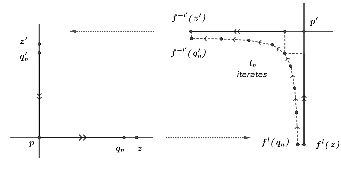
Figure 1. Construction of homoclinic orbits shadowing the heteroclinic cycle $p\leadsto p^{\prime}\leadsto p$.

In the third step we use the continuity of the holonomies. Notice also that the hyperbolicity at $p^{\prime}$ implies that the convergences $q_{n}\to z$, $f^{-l^{\prime}-r_{n}}(q_{n}^{\prime})\to p^{\prime}$ and $f^{-l^{\prime}-r_{n}}(z^{\prime})\to p^{\prime}$ are geometric with a rate which matches the strength of the base dynamics’s hyperbolicity. Hence because of the fiber-bunched assumption,

$$\lim_{n\to\infty}{\left\lVert A^{l+s_{n}}(q_{n})-A^{l+s_{n}}(z)\right\rVert}=0\quad\text{ and }$$

$$\lim_{n\to\infty}{\left\lVert A^{r_{n}+l^{\prime}}(f^{-l^{\prime}-r_{n}}(q_{n}^{\prime}))-A^{r_{n}+l^{\prime}}(f^{-l^{\prime}-r_{n}}(z^{\prime}))\right\rVert}=0.$$

Finally in the fourth step we use that

$$H^{s}_{f^{l}(z),p^{\prime}} =\lim_{n\to\infty}A(p^{\prime})^{-s_{n}}\,A^{s_{n}}(f^{l}(z)),$$

$$H^{u}_{p^{\prime},f^{-l^{\prime}}(z^{\prime})} =\lim_{n\to\infty}A^{r_{n}}(f^{-l^{\prime}-r_{n}}(z^{\prime}))\,A(p^{\prime})^{-r_{n}}.$$

This concludes the proof. ∎

Lemma 9.5.

If $f$ admits two periodic points $p,p^{\prime}\in\Lambda$, with periods $k$ and $k^{\prime}$ respectively, such that $A^{k}(p)$ is hyperbolic and $A^{k^{\prime}}(p^{\prime})$ is elliptic with eigenvalues which are not roots of unity with orders $1$, $2$, $3$, $4$, $6$ or $8$, then the cocycle satisfies pinching and twisting and hence has positive Lyapunov exponent.

Proof.

Working with the power $f^{kk^{\prime}}$, we can assume that $k=k^{\prime}=1$. Then $A(p)$ is hyperbolic and $A(p^{\prime})$ is elliptic. The pinching condition follows from the hyperbolicity of $A(p)$. We are left to prove the twisting condition for some transition map $\Phi$ associated with a homoclinic loop of $p$. Let $\{e_{1},e_{2}\}$ be the eigenvector basis of $A(p)$ and $\hat{e}_{1}$, $\hat{e}_{2}$ be the corresponding projective points. We want to prove that $\hat{\Phi}\hat{\,}e_{1}\neq\hat{e}_{2}$ and $\hat{\Phi}\,\hat{e}_{2}\neq\hat{e}_{1}$, where $\hat{\Phi}$ stands for the projective action of $\Phi$.

Take heteroclinic points $z$ and $z^{\prime}$ such that $z\in W^{u}_{\mathrm{loc}}(p)$ with $f^{l}(z)\in W^{s}_{\mathrm{loc}}(p^{\prime})$ and $z^{\prime}\in W^{s}_{\mathrm{loc}}(p)$ with $f^{-l^{\prime}}(z^{\prime})\in W^{u}_{\mathrm{loc}}(p^{\prime})$, where $l,l^{\prime}\in\mathbb{N}$. Set $\Psi_{0}:=\psi_{p,z,f^{l}(z),p^{\prime}}$ and $\Psi_{1}:=\psi_{p^{\prime},f^{-l^{\prime}}(z^{\prime}),z^{\prime},p}$. By Lemma 9.4 for every $m\in\mathbb{N}$, the $\operatorname{SL}(2,\mathbb{R})$ matrix $\Phi_{m}:=\Psi_{1}\,A(p^{\prime})^{m}\,\Psi_{0}$ can be approximated by transition maps of homoclinic loops of $p$. Let $\hat{e}_{i}^{\ast}:=\hat{\Psi}_{0}\,\hat{e}_{i}$ and $\hat{e}_{i}^{\sharp}:=\hat{\Psi}_{1}^{-1}\,\hat{e}_{i}$ for $i=1,2$. With this notation we need to find $m\in\mathbb{N}$ such that $\{\hat{e}_{1}^{\sharp},\hat{e}_{2}^{\sharp}\}\cap\hat{A}(p^{\prime})^{m}\{\hat{e}_{1}^{\ast},\hat{e}_{2}^{\ast}\}=\emptyset$. This suffices because any transition map of a homoclinic loop of $p$ that approximates $\Phi_{m}$ well enough satisfies the twisting condition. The assumption that the eigenvalues of $A(p^{\prime})$ are not roots of unity with orders $1$, $2$, $3$, $4$, $6$ or $8$ implies that the projective automorphism $\hat{A}(p^{\prime})$ is either aperiodic or else it has period $\geq 5$. We claim there exists $1\leq m\leq 5$ such that

$$\{\hat{e}_{1}^{\sharp},\hat{e}_{2}^{\sharp}\}\cap\hat{A}(p^{\prime})^{m}\{\hat{e}_{1}^{\ast},\hat{e}_{2}^{\ast}\}=\emptyset.$$ (9.2)

Let $\mathscr{O}(\hat{x}):=\{\hat{A}(p^{\prime})^{m}\hat{x}\colon m\in\mathbb{Z}\}$ denote the $\hat{A}(p^{\prime})$-orbit of a projective point $\hat{x}$. If $\mathscr{O}(\hat{e}_{1}^{\ast})\neq\mathscr{O}(\hat{e}_{2}^{\ast})$ these orbits are disjoint and it is not difficult to see that there are at least three $m\in\{1,\ldots,5\}$ such that (9.2) holds. Otherwise, if $\mathscr{O}(\hat{e}_{1}^{\ast})=\mathscr{O}(\hat{e}_{2}^{\ast})$ and this orbit is disjoint from $\{\hat{e}_{1}^{\sharp},\hat{e}_{2}^{\sharp}\}$ then (9.2) holds for all $m\in\mathbb{N}$. If $\mathscr{O}(\hat{e}_{1}^{\ast})=\mathscr{O}(\hat{e}_{2}^{\ast})$ and this orbit contains one element from $\{\hat{e}_{1}^{\sharp},\hat{e}_{2}^{\sharp}\}$ then (9.2) holds for three $m\in\{1,\ldots,5\}$. Finally, if $\mathscr{O}(\hat{e}_{1}^{\ast})=\mathscr{O}(\hat{e}_{2}^{\ast})$ and this orbit contains $\{\hat{e}_{1}^{\sharp},\hat{e}_{2}^{\sharp}\}$ then (9.2) holds for at least one $m\in\{1,\ldots,5\}$. This concludes the claim’s proof.

By Avila-Viana simplicity criterion, the positivity of the Lyapunov exponent follows. ∎

Since $\int v\,d\mu\neq 0$ without loss of generality we can assume that $\int v\,d\mu>0$. Take $0<\varepsilon<\frac{1}{2}\,\int v\,d\mu$. Next choose a Birkhoff generic point $q\in\Lambda$ for the averages of $v$ which is also an $f$-recurrent point near the fixed point $p$. More precisely choose $q\in\Lambda$ and $n\in\mathbb{N}$ such that $d(p,q)<\varepsilon/4$, $d(f^{n}(q),q)<\varepsilon/4$ and $\frac{1}{n}\,\sum_{j=1}^{n}v(T^{j}q)\geq\frac{4}{5}\,\int v\,d\mu$. If $\varepsilon$ is small enough by the shadowing property there exists a periodic point $q_{n}=f^{n}(q_{n})$ $\varepsilon/2$-near $q$. By the uniform continuity of $v$, if $\varepsilon$ is small enough we have $\frac{1}{n}\,\sum_{j=1}^{n}v(T^{j}q_{n})\geq\frac{2}{3}\,\int v\,d\mu$.

Thus by (9.1) provided $\lambda_{0}$ is small enough, we have for all $\bigl{|}\lambda\bigr{|}<\lambda_{0}$

$$\mathrm{tr}\left[\tilde{S}_{E,\lambda}^{n}(q_{n})\right]\geq 2\,\cos(n\kappa)-n\,\lambda\,\frac{\sin(n\kappa)}{\sin\kappa}\,\frac{1}{2}\,\int v\,d\mu\gg 2$$

which implies that $S_{E,\lambda}^{n}(q_{n})$ is hyperbolic.

Finally, Theorem 9.1 follows by Lemma 9.5. ∎

Acknowledgments

The first author was supported by Fundação para a Ciência e a Tecnologia, under the projects: UID/MAT/04561/2013 and PTDC/MAT-PUR/29126/2017. The second author has been supported by the CNPq research grants 306369/2017-6 and 313777/2020-9. The third author was also supported by Instituto Serrapilheira, grant “Jangada Dinâmica: Impulsionando Sistemas Dinâmicos na Região Nordeste”.

References

- [1] V. M. Alekseev and M. V. Yakobson, Symbolic dynamics and hyperbolic dynamic systems, Phys. Rep. 75 (1981), no. 5, 287–325.
- [2] A. Avila and M. Viana, Simplicity of Lyapunov spectra: a sufficient criterion, Port. Math. 64 (2007), 311–376.
- [3] Lucas Backes, Aaron Brown, and Clark Butler, Continuity of Lyapunov exponents for cocycles with invariant holonomies, J. Mod. Dyn. 12 (2018), 223–260.
- [4] V. Baladi, Gibbs states and equilibrium states for finitely presented dynamical systems, J. Statist. Phys. 62 (1991), no. 1-2, 239–256.
- [5] Alexandre Baraviera and Pedro Duarte, Approximating Lyapunov exponents and stationary measures, J. Dynam. Differential Equations 31 (2019), no. 1, 25–48. MR 3935134
- [6] Carlos Bocker-Neto and Marcelo Viana, Continuity of Lyapunov exponents for random two-dimensional matrices, Ergodic Theory and Dynamical Systems (2016), 1–30.
- [7] C. Bonatti, X. Gómez-Mont, and M. Viana, Généricité d’exposants de Lyapunov non-nuls pour des produits déterministes de matrices, Ann. Inst. H. Poincaré Anal. Non Linéaire 20 (2003), 579–624.
- [8] C. Bonatti and M. Viana, Lyapunov exponents with multiplicity 1 for deterministic products of matrices, Ergod. Th. & Dynam. Sys 24 (2004), 1295–1330.
- [9] Philippe Bougerol, Théorèmes limite pour les systèmes linéaires à coefficients markoviens, Probab. Theory Related Fields 78 (1988), no. 2, 193–221.
- [10] Philippe Bougerol and Jean Lacroix, Products of random matrices with applications to Schrödinger operators, Progress in Probability and Statistics, vol. 8, Birkhäuser Boston, Inc., Boston, MA, 1985.
- [11] J. Bourgain and M. Goldstein, On nonperturbative localization with quasi-periodic potential, Ann. of Math. (2) 152 (2000), no. 3, 835–879.
- [12] Jean Bourgain and Wilhelm Schlag, Anderson localization for Schrödinger operators on with strongly mixing potentials, Comm. Math. Phys. 215 (2000), no. 1, 143–175. MR 1800921 (2002d:81054)
- [13] Rufus Bowen, Equilibrium states and the ergodic theory of Anosov diffeomorphisms, revised ed., Lecture Notes in Mathematics, vol. 470, Springer-Verlag, Berlin, 2008, With a preface by David Ruelle, Edited by Jean-René Chazottes.
- [14] A. Boyarsky and P. Góra, Invariant measures and dynamical systems in one dimension, Probability and its Applications, Birkhäuser, 1997.
- [15] Victor Chulaevsky and Thomas Spencer, Positive lyapunov exponents for a class of deterministic potentials, Comm. Math. Phys. 168 (1995), no. 3, 455–466.
- [16] David Damanik, Schrödinger operators with dynamically defined potentials, Ergodic Theory Dynam. Systems 37 (2017), no. 6, 1681–1764.
- [17] Pedro Duarte and Silvius Klein, Lyapunov exponents of linear cocycles; continuity via large deviations, Atlantis Studies in Dynamical Systems, vol. 3, Atlantis Press, 2016.
- [18] by same author, Large deviations for products of random two dimensional matrices, Comm. Math. Phys. 375 (2020), no. 3, 2191–2257.
- [19] M. I. Gordin, The central limit theorem for stationary processes, Dokl. Akad. Nauk. SSSR 188 (1969), 1174–1176.
- [20] Sébastien Gouëzel and Luchezar Stoyanov, Quantitative Pesin theory for Anosov diffeomorphisms and flows, Ergodic Theory Dynam. Systems 39 (2019), no. 1, 159–200.
- [21] C. T. Ionescu-Tulcea and G. Marinescu, Théorie ergodique pour des classes d’operations non complètement continues, Annals of Math. 52 (1950), 140–147.
- [22] Svetlana Jitomirskaya and Xiaowen Zhu, Large deviations of the Lyapunov exponent and localization for the 1D Anderson model, Comm. Math. Phys. 370 (2019), no. 1, 311–324.
- [23] Émile Le Page, Théorèmes limites pour les produits de matrices aléatoires, Probability measures on groups (Oberwolfach, 1981), Lecture Notes in Math., vol. 928, Springer, Berlin-New York, 1982, pp. 258–303.
- [24] Émile Le Page, Régularité du plus grand exposant caractéristique des produits de matrices aléatoires indépendantes et applications, Ann. Inst. H. Poincaré Probab. Statist. 25 (1989), no. 2, 109–142.
- [25] Elaís C. Malheiro and Marcelo Viana, Lyapunov exponents of linear cocycles over Markov shifts, Stoch. Dyn. 15 (2015), no. 3, 1550020, 27.
- [26] Jerzy Ombach, Equivalent conditions for hyperbolic coordinates, Topology Appl. 23 (1986), no. 1, 87–90.
- [27] Kiho Park and Mark Piraino, Transfer operators and limit laws for typical cocycles, 2020.
- [28] H. Schaefer, Banach lattices and positive operators, Springer Verlag, 1974.
- [29] M. Shub, Global stability of dynamical systems, Springer Verlag, 1987.
- [30] El Hadji Yaya Tall and Marcelo Viana, Moduli of continuity for the Lyapunov exponents of random -cocycles, Trans. Amer. Math. Soc. 373 (2020), no. 2, 1343–1383.
- [31] Marcelo Viana, Almost all cocycles over any hyperbolic system have nonvanishing Lyapunov exponents, Ann. of Math. (2) 167 (2008), no. 2, 643–680.