Estimating energy levels of a three-level atom in single and multi-parameter metrological schemes

Abstract

Determining the energy levels of a quantum system is a significant task, for instance, to analyze reaction rates in drug discovery and catalysis or characterize the compatibility of materials. In this paper we exploit quantum metrology, the research field focusing on the estimation of unknown parameters exploiting quantum resources, to address this problem for a three-level system interacting with laser fields. The performance of simultaneous estimation of the levels compared to independent one is also investigated in various scenarios. Moreover, we introduce, the Hilbert-Schmidt speed (HSS), a special type of quantum statistical speed, as a powerful figure of merit for enhancing estimation of energy spectrum. This measure is easily computable, because it does not require diagonalization of the system state, verifying its efficiency in high-dimensional systems.

I Introduction

One of the most important applications of physical science is the measurement process whose goal is to associate a value with a physical quantity, resulting in an estimate of it. Together with each experimental estimate, an uncertainty, affecting the measurement result, appears. This statistical error can have two different natures: fundamental and technical. There are fundamental limits on uncertainty, such as those due to Heisenberg relations, that are imposed by physical laws. Conversely, the technical one is mostly represented by the accidental error, because of out-of-control imperfections in the measurement process. Since quantum mechanics is the most fundamental, predictive, and successful theory describing small scale phenomena, an investigation of the measurement process as well as the ultimate achievable precision bounds has to be done under the light of such theory [1, 2, 3, 4, 5, 6, 7, 8]. In fact, on the one hand, quantum theory determines fundamental limits on the estimate precision. On the other hand, for achieving such limits, quantum resources have to be used.

Interestingly, employing quantum systems to estimate unknown parameters overcomes the precision limits that can be, in principle, achieved by applying only classical resources. This idea is at the heart of the continuously growing research area of quantum metrology aiming at reaching the ultimate fundamental bounds on estimation precision by using quantum probes [9, 10, 11, 12, 13, 14, 15, 16, 17, 18, 19, 20, 21]. This field of research has attracted a great deal of interest in the last few years, leading to notable developments both theoretically and experimentally as reported in previous review papers concerning quantum phase estimation problems [22] optical metrology [23, 24, 25, 26, 27], multiparameter estimation scenario [28, 29, 30, 31], and metrological tasks performed by various physical systems [32, 33, 34].

Designing efficient quantum probes to achieve enhanced sensitivity has been recently generalized to a multi-parameter setting in which a set of spatially distributed quantum sensors is applied to simultaneously estimate a number of distinct parameters which cannot be measured directly or a function thereof [35, 36, 37, 38, 39], a setting which is relevant for a wide range of applications, including multi-dimensional field and gradient estimation [40, 41], nanoscale NMR [42], and quantum networks for atomic clocks [43] or astronomical imaging [44]. Here we investigate this strategy to enhance estimation of energy levels for a three-level system in which the cancellation of absorption may occur, impacting on important concepts and phenomena [45] such as lasing without inversion, enhancement of the index of refraction, and electromagnetically induced transparency.

Estimating and computing energy spectrum of a Hamiltonian are key problems in quantum mechanics. Many physical properties of a quantum system are primarily determined by its energy spectrum [46, 47]. For instance, the energy spectra of molecules give us important information on their dynamics and therefore an understanding of such spectra is necessary for molecular design [48]. Although the ground state problem has received considerable attention, comparing its theoretical and experimental findings with ones developed for finding the excited states of atomic and molecular systems, we see that the latter has experienced less development. This is despite the fact that it plays a key role in analyzing chemical reactions, a vital ingredient in the quest to discover new drugs and industrial catalysts [49, 47].

In this paper we estimate the energy spectrum of a Hamiltonian attributed to a three-level atom interacting with laser fields. We investigate the best strategies to extract the information about the energy levels in single and multi-parameter metrological schemes. Moreover, it is illustrated that the Hilbert-Schmidt speed, a quantifier of quantum statistical speed, can be used as a powerful tool to detect the atomic energy spectrum.

This paper is organized as follows: In Sec. II, we briefly review the theory of quantum metrology, The model is introduced in Sec. III. The independent estimation of the energy levels and application of Hilbert-Schmidt speed in this scenario are discussed in Sec. IV. Moreover, in Sec. V the simultaneous estimation of energy levels is investigated. Finally in Sec. VI, the main results are summarized.

II Estimation theory

Assuming that $\Phi_{\lambda}$ denotes a quantum channel depending on a set of parameters $\lambda=(\lambda_{1},...,\lambda_{n})$, we intend to estimate them through a quantum probe interacting with the channel. If the probe is prepared in the initial state $\rho$, the output $\rho_{\lambda}=\Phi_{\lambda}(\rho)$ should be measured to infer an estimation of the parameter. The measurement correspond to a positive operator valued measure (POVM), a set of positive operators $\{\varPi_{x}\}$ satisfying the relations $\sum\limits_{x}\varPi_{x}\varPi_{x}^{\dagger}=\mathcal{I}$ and $p(x|\lambda)\equiv\prod\limits_{i}p(x_{i}|\lambda)=\text{Tr}[\varPi_{x}\rho_{\lambda}]$, representing the probability distribution for results $x=(x_{1},...,x_{M})$ of the measurements implemented $M$-times. In addition, according to achieved results of the measurement, the parameters can be estimated by using an estimator $\tilde{\lambda}(x)=(\tilde{\lambda}_{1}(x),,...,\tilde{\lambda}_{n}(x))$. When $E(\tilde{\lambda})\equiv\sum\limits_{x}p(x|\lambda)\tilde{\lambda}(x)=\lambda$ [i.e., its expected value coincides with the true value of the parameter(s)], we call it an unbiased estimator [50, 51]. Physically, the results $x$ are obtained by measuring a related observable $X$ whose eigenvalues constitute a discrete or continuous spectrum. If the eigenvalue spectrum of that observable is continuous, the summation in the above equation must be replaced by an integral.

The efficiency of an estimator can be quantified by the covariance matrix, $\text{Cov}[\tilde{\lambda}]$, capturing both the variance of—and therefore the error on—each of the individual parameters, as well as the covariance—and hence some indication of the correlation—between them [52]. The Cramér-Rao bound states that, for all unbiased estimators $\tilde{\lambda}$, the covariance matrix whose elements are defined as $\text{Cov}[\tilde{\lambda}]_{ij}=E[\tilde{\lambda}_{i}\tilde{\lambda}_{j}]-E[\tilde{\lambda}_{i}]E[\tilde{\lambda}_{j}]$ satisfies the following inequality [53, 54]

$$\text{Cov}[\tilde{\lambda}]\geq\dfrac{1}{M}\textbf{I}(\lambda)^{-1},$$ (1)

in which $M$ denotes the number of experimental runs. Moreover, $\textbf{I}^{-1}$ represents the inverse of the classical Fisher information (FI) matrix whose elements are defined as follows [15, 51]

$$\text{I}_{ij}=\sum\limits_{x}\dfrac{1}{p(x|\lambda)}\dfrac{\partial p(x|\lambda)}{\partial\lambda_{i}}\dfrac{\partial p(x|\lambda)}{\partial\lambda_{j}}.$$ (2)

In order to compute the quantum Fisher information matrix (QFIM) F defined as the upper bound of the classical one via the matrix inequality $\textbf{F}\geq\textbf{I}$ [55], we first require to obtain the Symmetric Logarithmic Derivative (SLD) $L_{\lambda_{j}}~{}~{}(j=1,2,...,p)$ satisfying the operator equation

$$\frac{\partial\rho(\lambda)}{\partial\lambda_{j}}=\dfrac{1}{2}[L_{\lambda_{j}}\rho(\lambda)+\rho(\lambda)L_{\lambda_{j}}],$$ (3)

where $\rho$ denotes the density operator of the system. In the next step, the elements of QFIM can be easily computed by

$$F_{ij}=\frac{1}{2}\text{Tr}[\rho(L_{\lambda_{i}}L_{\lambda_{j}}+L_{\lambda_{j}}L_{\lambda_{i}})].$$ (4)

The QFI associated with the ultimate precision in the multi-parameter estimation strategy provides a lower bound on the covariance matrix, i.e.,

$$\text{Cov}[\tilde{\lambda}]\geq\dfrac{1}{M}\textbf{F}(\lambda)^{-1},$$ (5)

which is called the Cramer-Rao bound (QCRB) [15].

If we aim at estimating each parameter independently (i.e., single-parameter estimation), the inequality reads [56, 50]

$$(\delta\lambda_{j})_{i}\geq\dfrac{1}{MF_{jj}},$$ (6)

in which $\delta\lambda_{j}\equiv\text{Var}(\tilde{\lambda}_{j})\equiv E(\tilde{\lambda}_{j}^{2})-E(\tilde{\lambda}_{j})^{2}$ and $F_{jj}\equiv F(\lambda_{j})$, denoting the QFI associated with the parameter $\lambda_{j}$, is given by

$$F_{\lambda_{j}}=\text{Tr}[\rho(\lambda)L_{\lambda_{j}}^{2}].$$ (7)

In the independent estimation scenario, a lower bound on the total variance of all parameters, which should be estimated, can be computed by:

$$\delta_{i}\equiv\sum\limits_{j}(\delta\lambda_{j})_{i}\equiv\sum_{j}\dfrac{1}{MF_{jj}}$$ (8)

However, if we want to estimate the parameters simultaneously, the inequality for the variance of each parameter is obtained as [50]

$$(\delta\lambda_{j})_{s}\geq\dfrac{[\textbf{F}(\lambda)^{-1}]_{jj}}{M},$$ (9)

Accordingly, when there exists nonzero off-diagonal elements in the QFI matrix, the uncertainty bounds for simultaneous and independent estimations may be different from each other. Moreover, in order to obtain a lower bound on the total variance of all parameters of interest, we can take the trace of both sides of Eq. (5), leading to [53]

$$\delta_{s}\equiv\sum\limits_{j}(\delta\lambda_{j})_{s}\equiv\text{Tr}\big{(}\text{Cov}[\tilde{\lambda}]\big{)}\geq\dfrac{1}{M}\text{Tr}\big{(}\textbf{F}(\lambda)^{-1}\big{)}.$$ (10)

In the single parameter scenario, using the eigenvectors of the SLD operator as the POVM, one achieve that $\text{I}=\text{F}$ and hence the QCRB (6) can be saturated [57]. However, in the simultaneous estimation of parameters the procedure may be more challenging than the individual one. Since the optimal measurement for a given parameter can be constructed by projectors corresponding to the eigenbasis of the SLD, we can consequently conclude that when $\forall~{}(\lambda_{j},\lambda_{k})\in\lambda:~{}[L_{\lambda_{j}},L_{\lambda_{k}}]=0$, one can find a common eigenbasis for all SLDs and hence a common measurement optimal from the point of view of extracting information on all parameters simultaneously. It should be noted tat it is only a sufficient but not a necessary condition. In detail, if the SLDs do not commute, this does not necessarily indicate that it is not possible to simultaneously extract information on all parameters with precision matching that of the individual scenario for each [57].

There is a weaker condition stating that the multiparameter QCRB can be saturated provided that [57, 58]

$$\text{Tr}(\rho[L_{i},L_{k}])=0.$$ (11)

Therefore, not the commutator itself but only its expectation value on the probe state is required to vanish.

In order to compare the performance of simultaneous estimation with that of individual one, we define the ratio [52]:

$$R=\frac{\Delta_{\text{i}}}{\Delta_{\text{s}}},$$ (12)

where the minimal total variances in the individual and simultaneous estimations are denoted by, respectively, $\Delta_{\text{i}}=\sum_{j}\dfrac{1}{MF_{jj}}$ and $\Delta_{\text{s}}=\dfrac{1}{Mp}\text{Tr}\big{(}\textbf{F}(\lambda)^{-1}\big{)}$ in which $p$ denotes the number of parameters to be estimated. In fact, a simultaneous estimation scheme requires fewer resources than the corresponding independent estimation scheme by a factor of the number of parameters to be estimated. Inserting $p$ in the definition of $\Delta_{\text{s}}$ is required to account for this reduction in resources. The measure changes in the range of $0\leq R\leq p$ where R$\mathrm{>}$1 indicates the better performance of multi-parameter estimation rather than the single one. Considering a single repetition of the measurement, we set $M=1$ throughout this paper.

III Model

We consider a three-level atom interacting with two electromagnetic fields of frequencies ${\nu}_{1}$ and ${\nu}_{2}$ (see Fig. 1). It is assumed the atom is in the ${\Lambda}$ configuration in which two lower levels $\left.\mathrm{\textrm{$|$}}b\right\rangle$ and$\left.\mathrm{\textrm{$|$}}c\right\rangle$ are coupled to a single upper level$\left.\mathrm{\textrm{$|$}}a\right\rangle$.

Figure 1: Three-level atom in the $\Lambda$ configuration subject to two fields of frequencies $\nu_{1}$ and $\nu_{2}$.

In the rotating-wave approximation, the Hamiltonian of the system is given by [45]:

$$\mathcal{H}={\mathcal{H}}_{0}+{\mathcal{H}}_{1}$$ (13)

where

$$\left.{\mathcal{H}}_{0}\mathrm{=}\mathrm{\hbar}{\mathrm{\textrm{{\hbox{\omega}}}}}_{a}\mathrm{\textrm{{\hbox{|}}}}a\right\rangle\left\langle a\mathrm{\textrm{{\hbox{|}}}}\mathrm{+}\left.\mathrm{\hbar}{\mathrm{\textrm{{\hbox{\omega}}}}}_{b}\mathrm{\textrm{{\hbox{|}}}}b\right\rangle\left\langle b\mathrm{\textrm{{\hbox{|}}}}\left.\mathrm{+}\mathrm{\hbar}{\mathrm{\textrm{{\hbox{\omega}}}}}_{c}\mathrm{\textrm{{\hbox{|}}}}c\right\rangle\left\langle c\mathrm{\textrm{{\hbox{|}}}}\right.\right.\right.$$ (14)

denotes the unperturbed Hamiltonian having eigenvalues $\left\{\hbar\omega_{a},\hbar\omega_{b},\hbar\omega_{c}\right\}$, and

$${\mathcal{H}}_{1}\mathrm{=}{\mathrm{-}\frac{\mathrm{\hbar}}{\mathrm{2}}\mathrm{(}{\mathrm{\textrm{{\hbox{\Omega}}}}}_{R1}e^{-i{\textrm{{\hbox{\phi}}}}_{1}}e^{-i{\textrm{{\hbox{\nu}}}}_{1}t}\left.\mathrm{\textrm{{\hbox{|}}}}a\right\rangle\left\langle b\mathrm{\textrm{{\hbox{|}}}}\mathrm{+}{\mathrm{\textrm{{\hbox{\Omega}}}}}_{R2}e^{-i{\textrm{{\hbox{\phi}}}}_{2}}e^{-i{\textrm{{\hbox{\nu}}}}_{2}t}\left.\mathrm{\textrm{{\hbox{|}}}}a\right\rangle\left\langle c\mathrm{\textrm{{\hbox{|}}}}\right.\mathrm{)+H.c}\right.}$$ (15)

describes the interaction between the atom and fields. Moreover, ${\mathrm{\textrm{$\Omega$}}}_{R1}e^{-i{\textrm{$\phi$}}_{1}}$ and ${\mathrm{\textrm{$\Omega$}}}_{R2}e^{-i{\textrm{$\phi$}}_{2}}$ represent the complex Rabi frequencies associated with the coupling of the field modes of the frequencies ${\nu}_{1}$ and ${\nu}_{2\ }$ to the atomic transitions$\left.\mathrm{\textrm{$|$}}a\right\rangle$$\mathrm{\to}$$\left.\mathrm{\textrm{$|$}}b\right\rangle$ and$\left.\mathrm{\textrm{$|$}}a\right\rangle$$\mathrm{\to}$$\left.\mathrm{\textrm{$|$}}c\right\rangle$, respectively. We consider in which only $\left.\mathrm{\textrm{$|$}}a\right\rangle$$\mathrm{\to}$$\left.\mathrm{\textrm{$|$}}b\right\rangle$ and$\left.\mathrm{\textrm{$|$}}a\right\rangle$$\mathrm{\to}$$\left.\mathrm{\textrm{$|$}}c\right\rangle$ transitions are dipole allowed.

Preparing the system in the initial atomic state

$$\left.\mathrm{\textrm{{\hbox{|}}}}\textrm{{\hbox{\psi}}}(0)\right\rangle\mathrm{\ }={\mathrm{cos}\left(\frac{\textrm{{\hbox{\theta}}}}{2}\right)\left.\mathrm{\textrm{{\hbox{|}}}}b\right\rangle\ }+{\mathrm{sin}\left(\frac{\textrm{{\hbox{\theta}}}}{2}\right)\left.e^{-i\textrm{{\hbox{\psi}}}}\mathrm{\textrm{{\hbox{|}}}}c\right\rangle\ },$$ (16)

which is a superposition of the two lower levels $\left\{\left.\mathrm{\textrm{$|$}}b\right\rangle,\left.\mathrm{\textrm{$|$}}c\right\rangle\right\}$, and assuming that the fields to be resonant with the $\left.\mathrm{\textrm{$|$}}a\right\rangle$$\mathrm{\to}$$\left.\mathrm{\textrm{$|$}}b\right\rangle$ and the$\left.\mathrm{\textrm{$|$}}a\right\rangle$$\mathrm{\to}$$\left.\mathrm{\textrm{$|$}}c\right\rangle$ transitions respectively, i.e, ${\textrm{$\omega$}}_{ab}\mathrm{=}{\textrm{$\nu$}}_{1}$ and ${\textrm{$\omega$}}_{ac}\mathrm{=}{\textrm{$\nu$}}_{2}$, we find that the evolved state of the system is given by [45, 54]

$$\left.\mathrm{\textrm{{\hbox{|}}}}\textrm{{\hbox{\psi}}}(t)\right\rangle=\ \left.c_{a}\left(\mathrm{t}\right)e^{\mathrm{-}\mathrm{i}{\mathrm{\textrm{{\hbox{\omega}}}}}_{a}\mathrm{t}}\mathrm{\textrm{{\hbox{|}}}}a\right\rangle+\left.c_{b}\left(\mathrm{t}\right)e^{\mathrm{-}\mathrm{i}{\mathrm{\textrm{{\hbox{\omega}}}}}_{b}\mathrm{t}}\mathrm{\textrm{{\hbox{|}}}}b\right\rangle+\left.c_{c}\left(\mathrm{t}\right)e^{\mathrm{-}\mathrm{i}{\mathrm{\textrm{{\hbox{\omega}}}}}_{c}\mathrm{t}}\mathrm{\textrm{{\hbox{|}}}}c\right\rangle,$$ (17)

where

$$c_{a}=\frac{i~{}\text{sin}(\mathrm{\textrm{{\hbox{\Omega}}}}t/2)}{2}[{\mathrm{\textrm{{\hbox{\Omega}}}}}_{R1}e^{-i{\textrm{{\hbox{\phi}}}}_{1}}\mathrm{cos}\mathrm{}(\frac{\textrm{{\hbox{\theta}}}}{2})+{\mathrm{\textrm{{\hbox{\Omega}}}}}_{R2}e^{-i{(\textrm{{\hbox{\phi}}}}_{2}+\textrm{{\hbox{\psi}}})}\mathrm{sin}\mathrm{}(\frac{\textrm{{\hbox{\theta}}}}{2})]$$ (18)

$$c_{b}=\frac{1}{{\mathrm{\textrm{{\hbox{\Omega}}}}}^{2}}\{\left[{\mathrm{\textrm{{\hbox{\Omega}}}}}^{2}_{R2}+{\mathrm{\textrm{{\hbox{\Omega}}}}}^{2}_{R1}\text{cos}\left(\frac{\mathrm{\textrm{{\hbox{\Omega}}}}t}{2}\right)\right]{\mathrm{cos}\left(\frac{\textrm{{\hbox{\theta}}}}{2}\right)\ }-2{\mathrm{\textrm{{\hbox{\Omega}}}}}_{R1}{\mathrm{\textrm{{\hbox{\Omega}}}}}_{R2}e^{i{(\textrm{{\hbox{\phi}}}}_{1}-{\textrm{{\hbox{\phi}}}}_{2}-\textrm{{\hbox{\psi}}})}{\text{sin}}^{2}\left(\frac{\mathrm{\textrm{{\hbox{\Omega}}}}t}{4}\right)\text{sin}\left(\frac{\mathrm{\textrm{{\hbox{\theta}}}}}{2}\right)\}$$ (19)

$$c_{c}=\frac{1}{{\mathrm{\textrm{{\hbox{\Omega}}}}}^{2}}\{-2{\mathrm{\textrm{{\hbox{\Omega}}}}}_{R1}{\mathrm{\textrm{{\hbox{\Omega}}}}}_{R2}e^{-i{(\textrm{{\hbox{\phi}}}}_{1}-{\textrm{{\hbox{\phi}}}}_{2})}{\text{sin}}^{2}\left(\frac{\mathrm{\textrm{{\hbox{\Omega}}}}t}{4}\right)\text{cos}\left(\frac{\mathrm{\textrm{{\hbox{\theta}}}}}{2}\right)+\left[{\mathrm{\textrm{{\hbox{\Omega}}}}}^{2}_{R1}+{\mathrm{\textrm{{\hbox{\Omega}}}}}^{2}_{R2}\text{cos}\left(\frac{\mathrm{\textrm{{\hbox{\Omega}}}}t}{2}\right)\right]{e^{-i\textrm{{\hbox{\psi}}}}\mathrm{sin}\left(\frac{\textrm{{\hbox{\theta}}}}{2}\right)\ }\}$$ (20)

in which $\mathrm{\textrm{$\Omega$}}\mathrm{=}{{\mathrm{(}\mathrm{\textrm{$\Omega$}}}^{2}_{R1}+{\mathrm{\textrm{$\Omega$}}}^{2}_{R2})}^{\frac{1}{2}}$. In the special case that

$$\Omega_{\mathrm{R1}}=\Omega_{\mathrm{R2}},~{}~{}\theta=\pi/2,~{}~{}\alpha=\phi_{1}-\phi_{2}-\psi=\pm\pi,$$ (21)

the coherent trapping occurs, because

$$c_{a}(t)=0,~{}~{}c_{b}(t)=\frac{1}{\sqrt{2}},~{}~{}c_{c}(t)=\frac{1}{\sqrt{2}}\text{e}^{-i\psi},$$ (22)

meaning that the population is trapped in the lower states and there is no absorption even in the presence of the applied fields. This phenomenon arises from the quantum interference between the two transitions from the two lowest state to the uppermost state. Coherent population trapping (CPT) can easily be observed in the D lines of alkali atoms (Cs, Rb, K, etc.) [59, 60]. CPT resonance signals have been widely studied for precision sensing with potential applications in microwave atomic clocks based on vapor cells and cold atoms, magnetometers, high-resolution spectroscopy, atomic interferometers, and phase-sensitive amplification [61, 62, 63, 64, 65, 66].

In this paper we show that CPT may play an important role in estimation of the energy levels of an atomic system. We set $\theta=\pi/2$ throughout this paper.

IV Single parameter estimation

In this section, computing the QFIs, we investigate the single parameter estimation for detecting energy levels of a three level atom in two different regimes: (a) different Rabi frequencies (${\mathrm{\textrm{$\Omega$}}}_{R1}\neq$ ${\mathrm{\textrm{$\Omega$}}}_{R2}$), and (b) equal Rabi frequencies (${\mathrm{\textrm{$\Omega$}}}_{R1}=$ ${\mathrm{\textrm{$\Omega$}}}_{R2}$). The analytical expressions of the QFIs are given in the Appendix. It is interesting to see that the QFIs are independent of the energy levels as well as the transition frequencies. Moreover the QFIs do not explicitly depend on the laser phases $(\phi_{1},\phi_{2})$ and the initial phase $\psi$. Instead, they rise in defining parameter $\alpha=\phi_{1}-\phi_{2}-\psi$ appearing in the QFIs expressions. Accordingly the effects of the laser phases on the estimation of the energy levels can be controlled by changing phase $\psi$ encoded into the initial state of the system.

IV.1 Single parameter estimation with respect to ${\bm{\mathrm{\textrm{$\omega$}}}}_{\bm{a}}$

For the case of equal Rabi frequencies $\mathrm{(}{\mathrm{\textrm{$\Omega$}}}_{R1}={\mathrm{\textrm{$\Omega$}}}_{R2}=\mathrm{\textrm{$\Omega$}}\mathrm{{}^{\prime})}$, the dynamics of the QFI with respect to ${\mathrm{\textrm{$\omega$}}}_{a}$ is plotted in Fig. 2 for different values of the parameter $\alpha$.

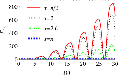
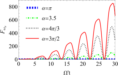
Figure 2: The dynamics of ${{\mathrm{F}}}_{{{\mathrm{\textrm{$\omega$}}}}_{{\mathrm{a}}}}$ as a function of the scaled time ${\mathrm{t}}{\mathrm{\textrm{$\Omega$}}}{\mathrm{{}^{\prime}}}$ for ${\textrm{$\theta$}}{=}{\textrm{$\pi$}}{/}{2}$ and various values of $\alpha$, in equal Rabi frequencies regime ${{\mathrm{\textrm{$\Omega$}}}}_{{R}{1}}{=}{{\mathrm{\textrm{$\Omega$}}}}_{{R}{2}}{=}{\mathrm{\textrm{$\Omega$}}}{\mathrm{{}^{\prime}}}$.

The maximized QFI, obtained for $\textrm{$\alpha$}=\bm{\textrm{$\pi$}}\bm{/}\bm{2}$ and $\textrm{$\theta$}=\bm{\textrm{$\pi$}}\bm{/}\bm{2}$, is given by

$${F}^{\text{max}}_{{\textrm{{\hbox{\omega}}}}_{\mathrm{a\ }}}=\begin{array}[]{c}\frac{1}{2}t^{2}{\mathrm{sin}}^{2}(\frac{t{\mathrm{\textrm{$\Omega$}}}^{\prime}}{\sqrt{2}})(\mathrm{cos}(\sqrt{2}t{\mathrm{\textrm{$\Omega$}}}^{\prime})+3\end{array}).$$ (23)

Therefore at times ${\mathrm{\textrm{$\Omega$}}}^{\prime}t=\sqrt{2}\pi$ where the QFI becomes equal to zero and hence the estimation fails. Accordingly, the Rabi frequency can be used as an efficient tool to shift the moments at which the the single upper level is hidden from measuring devices.

Moreover, the QFI vanishes for $\theta=\pi/2$ and $\alpha=\pi$, showing that no information about the energy of the upper excited state can be extracted from the qutrit when the coherent trapping occurs. Therefore, when the population is trapped in the lower states, the information about the single excited state becomes unaccessible. Distancing from the coherent trapping mode, for example by decreasing $\alpha$ from $\pi$ to $\pi/2$ (see Fig. 2) or increasing it in the range $[\pi/2,3\pi/2]$ (see Fig. 2), we can enhance the parameter estimation of the upper energy level.

IV.2 Single parameter estimation with respect to ${\bm{\mathrm{\textrm{$\omega$}}}}_{\bm{b}}$

Another interesting scenario is quantum estimation of the lowest level energy $\omega_{b}$. Figure 3 exhibits the QFI dynamics in the different Rabi frequencies regime (${\mathrm{\textrm{$\Omega$}}}_{R1}\neq$ ${\mathrm{\textrm{$\Omega$}}}_{R2}$) for various values of ${\mathrm{\textrm{$\Omega$}}}_{R2}$. As observed in Figs. 3 and 3, an increase in the Rabi frequency ${\mathrm{\textrm{$\Omega$}}}_{R2}$ decreases the amplitude of the time oscillations of the QFI such that for large values of ${\mathrm{\textrm{$\Omega$}}}_{R2}$, ${\mathrm{QFI}}_{{\mathrm{\textrm{$\omega$}}}_{\mathrm{a}}}$ monotonically increases with time and the best estimation occurs. In particular, we find that

$$\lim_{\Omega_{\mathrm{R2}}\to\infty}F_{\omega_{b}}=t^{2}.$$ (24)

Because the Rabi frequency is proportional to the field amplitude, we find that intensifying the field, being resonant with the allowed transition between the intermediate levels, one can achieve the best precision in quantum estimation of the lowest level energy. This situation is similar to what occurs in electromagnetically induced transparency in which one of the two fields, driving the upper two levels, is intense whereas the other is weak and can be treated as a probe field. Under appropriate parametric conditions, it is possible to show that the system, independently of the initial condition, evolves to a stationary state in which it is transparent (zero absorption) to the probe field. Therefore, the population of the lower levels increase with time, leading to a monotonous increase in precision of estimating the ground state energy of the atom.

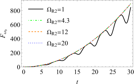
Figure 3: The time variation of ${{\mathrm{F}}}_{{{\mathrm{\textrm{$\omega$}}}}_{{\mathrm{b}}}}$ for ${\mathrm{\ }}{{\mathrm{\textrm{$\Omega$}}}}_{{R}{1}}{\mathrm{=}}{\mathrm{1}}$, ${\textrm{$\alpha$}}{=}{\textrm{$\pi$}}{/}{2}$, ${\textrm{$\theta$}}{=}{\textrm{$\pi$}}{/}{2}$ and various values of ${{\mathrm{\textrm{$\Omega$}}}}_{{R}{2}}$.

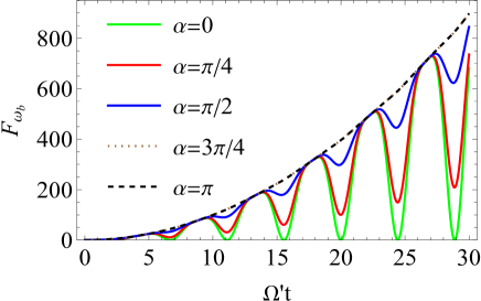
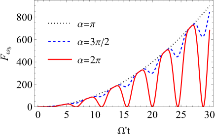
Figure 4: The variation of ${{\mathrm{F}}}_{{{\mathrm{\textrm{$\omega$}}}}_{{\mathrm{b}}}}$ as a function of the scaled time ${\mathrm{t}}{\mathrm{\textrm{$\Omega$}}}{\mathrm{{}^{\prime}}}$ for ${\textrm{$\theta$}}{=}{\textrm{$\pi$}}{/}{2}$ and different values of $\alpha$ in the equal Rabi frequencies regime, i.e., ${{\mathrm{\textrm{$\Omega$}}}}_{{R}{1}}{=}{{\mathrm{\textrm{$\Omega$}}}}_{{R}{2}}{=}{\mathrm{\textrm{$\Omega$}}}{\mathrm{{}^{\prime}}}$.

In Figs. 4 and 4, we show the time evolution of the QFI in equal Rabi frequencies $\mathrm{(}{\mathrm{\textrm{$\Omega$}}}_{R1}={\mathrm{\textrm{$\Omega$}}}_{R2}=\mathrm{\textrm{$\Omega$}}\mathrm{{}^{\prime})}$ for different values of $\alpha$. We observe that the best estimation is realized when the coherent trapping occurs, leading to the following expression for the optimal QFI:

$$F^{max}_{{\textrm{{\hbox{\omega}}}}_{\mathrm{b\ }}}=t^{2},$$ (25)

verifying monotonic enhancement of parameter estimation with time.

IV.3 Single parameter estimation with respect to ${\bm{\mathrm{\textrm{$\omega$}}}}_{\bm{c}}$

Investigating the single-parameter estimation with respect to $\omega_{c}$, we find that an increase in the Rabi frequency ${\mathrm{\textrm{$\Omega$}}}_{R1}$ decreases the amplitude of the time oscillations of the QFI such that for large values of ${\mathrm{\textrm{$\Omega$}}}_{R1}$, we have

$$\lim_{\Omega_{\mathrm{R1}}\to\infty}F_{\omega_{c}}=t^{2}.$$ (26)

As discussed in the previous section the Rabi frequency is proportional to the field amplitude, and hence we conclude that intensifying the field, being resonant with the allowed transition between the lower ground and upper excited states, we can optimally estimate the energy of the intermediate level.

Again, we find that in equal Rabi frequencies regime when the coherent trapping is realized, the best estimation is achieved such that the optimal QFI is given by:

$$F^{\text{max}}_{{\textrm{{\hbox{\omega}}}}_{\mathrm{c\ }}}=t^{2},$$ (27)

showing monotonic enhancement of parameter estimation with time.

IV.4 Hilbert-Schmidt as an efficient tool for estimation of energy levels

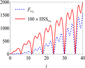
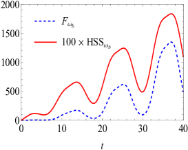
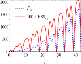
Figure 5: Comparison between dynamics of quantum Fisher information $F_{\omega_{i}}$ and Hilbert-Schmidt speed $HSS_{\omega_{i}}$ (amplified by 100 times) for ${{\mathrm{\textrm{$\Omega$}}}}_{{R}{1}}{\mathrm{=}}{\mathrm{0}}.{\mathrm{32,}}$ ${{\mathrm{\textrm{$\Omega$}}}}_{{R}{2}}=1,$  ${{\mathrm{\textrm{$\phi$}}}}_{{1}}{\mathrm{=}}{\mathrm{1}},{{\mathrm{\textrm{$\phi$}}}}_{{2}}{\mathrm{=}}{\mathrm{1}},{\mathrm{\textrm{$\psi$}}}{=}{2}{\textrm{$\pi$}}{\ }{and}{\ }{\textrm{$\theta$}}{=}{\textrm{$\pi$}}{/}{2}.$

Given quantum state $\rho(\varphi)$, one can define the Hilbert–Schmidt speed (HSS) given by [67, 68]

$$HSS_{{\varphi}}(\rho\big{)}=\sqrt{\frac{1}{2}\text{Tr}\bigg{[}\bigg{(}\dfrac{d\rho(\varphi)}{d\varphi}\bigg{)}^{2}\bigg{]}},$$ (28)

is a special quantifer of quantum statistical speed associated with parameter $\varphi$. It can be easily computed without diagonalization of $\text{d}\rho(\varphi)/\text{d}\varphi$.

In Ref. [69], the HSS has been introduced as a powerful figure of merit for enhancing quantum phase estimation in an open quantum system made of $n$ qubits. More generally, because both QFI and HSS are quantum statistical speeds associated, respectively, with the Bures and Hilbert–Schmidt distances, it is reasonable to explore how they can be related to each other. Accordingly, here we investigate the application of the HSS in detecting the energy levels of our three-level system.

The dynamical comparison between the the QFI and HSS computed with respect to the same parameters, is performed numerically. In particular, we show in Fig. 5 that both the QFI and HSS dynamics simultaneously exhibit an oscillatory behavior such that their maximum and minimum points exactly coincide. These plots qualitatively verifies that the HSS can detect exactly the times at which the best estimation of the energy levels occurs (maximum of the QFI).

Because the HSS is an easily computable quantity having the advantage of avoiding diagonalization of the evolved density matrix, our result shows that it can be used as a convenient as well as powerful figure of merit in estimating the energy levels.

V Multi-parameter estimation of energy levels

As we discussed in Sec. II if $\forall~{}(\omega_{i},\omega_{j}):~{}[L_{\omega_{i}},L_{\omega_{j}}]=0$ where $i,j=a,b,c$, then there is no additional difficulty in extracting optimal information from a state on all energy levels simultaneously. Although the SLDs associated with the parameters $\omega_{a},\omega_{b},\omega_{c}$ do not satisfy the above relation, we fortunately find that the commutation condition (11) holds in our model. This means that there is a single measurement which is jointly optimal for extracting information on all energy levels, which should be estimated simultaneously, from the output state, ensuring the asymptotic saturability of the QCRB.

V.1 Single-qutrit scenario

Employing a single-qutrit system in the estimation process, we analyze the variance of estimating one of the atomic energy levels when it is estimated simultaneously. In the equal Rabi frequencies regimes, simultaneously estimating $\omega_{a}$ and $\omega_{b}$, we find that the qualitative results extracting for estimation variance of $\omega_{a}$ ($\omega_{b}$), are exactly similar to ones achieved from Fig. 2 (4) for single parameter estimation, i.e.; (a) Distancing from the coherent trapping mode, we can enhance the parameter estimation of the upper energy level; (b) The best estimation of the ground state energy is realized when the coherent trapping occurs.

V.2 Two-qutrit scenario

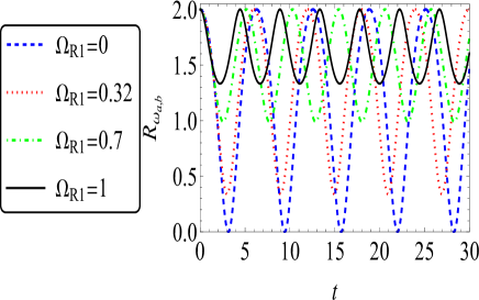
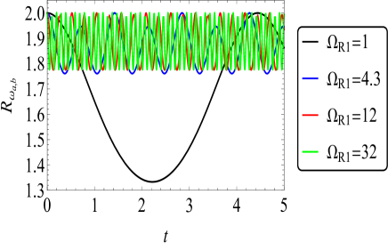
Figure 6: The dynamics of performance ratio $R_{{\textrm{$\omega$}}_{\mathrm{a,b}}}$, computed for simultaneous estimation of $\omega_{a}$ and $\omega_{b}$, for ${\textrm{$\alpha$}},{\textrm{$\theta$}}{=}{\textrm{$\pi$}}{/}{2}$, $\Omega_{\mathrm{R2}}=1$ and various values of ${{\mathrm{\textrm{$\Omega$}}}}_{{R}{1}}$.

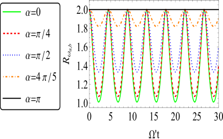
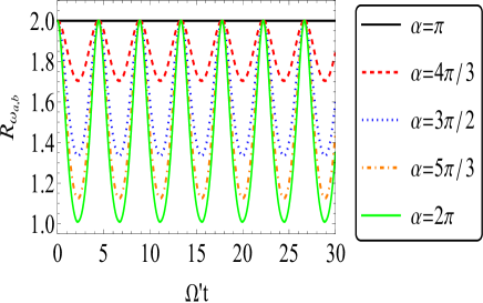
Figure 7: The variation of performance ratio $R_{{\textrm{$\omega$}}_{\mathrm{a,b}}}$, calculated for simultaneous estimation of $\omega_{a}$ and $\omega_{b}$, as a function of the scaled time $\Omega^{{}^{\prime}}t$ for $\theta$${=}{\textrm{$\pi$}}{/}{2}$ and different values of $\alpha$ in the equal Rabi frequencies regime.

It is clear that when a single qutrit is applied for estimation, no advantage is attained by simultaneously estimating the parameters. In the second strategy we are interested to investigate what happens if we increase the number of resources. In detail, we assume that two uncorrelated qubtrits are applied in the estimation scheme. In the individual estimation one of which is used to estimate $\omega_{i}$ and the other is used to estimate $\omega_{j}$ where $i,j=a,b,c$, leading to the minimal total variance on both the parameters as $\Delta_{i}(2)=(1/F_{ii})+(1/F_{jj})$. However, in the simultaneous estimation each of these qutrits is used to estimate both parameters, and hence the results from the two qutrits can be classically combined to achieve $\Delta_{s}(2)=\frac{1}{2}\Delta_{s}(1)=\frac{1}{2}([\textbf{F}(\lambda)^{-1}]_{ii}+[\textbf{F}(\lambda)^{-1}]_{jj})=\frac{1}{2}\text{Tr}(\textbf{F}^{-1})$.

V.2.1 Simultaneous estimation of $\omega_{a}$ and $\omega_{b}$

In the first interesting scenario in which the lowest and highest energy levels, i.e., $\{\omega_{a},\omega_{b}\}$, should be estimated, we see that the ratio $R_{\omega_{a,b}}$ may become greater than one by an increase in the Rabi frequency $\Omega_{\mathrm{R1}}$ (see Fig. 6). Therefore, imposing an intense field resonant with the allowed transition between the lower ground and upper excited states, we observe that the simultaneous strategy always advantageous than the individual one.

If the off-diagonal elements of the QFIM are zero, the parameters of interest would are statistically independent, meaning that the indeterminacy of one of which does not affect the error on estimating the others. Under this condition $\Delta_{s}(2)=\frac{1}{2}\Delta_{i}(2)$, and hence the ratio $R=\Delta_{i}/\Delta_{s}$ have a maximum value of $2$, indicating complete superiority of the simultaneous scheme. Figure 7 illustrates that in the equal Rabi frequencies regime when the coherent trapping occurs, the QFIM becomes diagonal. Consequently, $R_{\omega_{a,b}}$ achieved its maximum value and hence the superiority of the simultaneous estimation is completely realized. Deviating from the coherent trapping by changing $\alpha$, we find that the efficiency of the simultaneous estimation compared to the independent one decreases.

V.2.2 Simultaneous estimation of $\omega_{a}$ and $\omega_{c}$

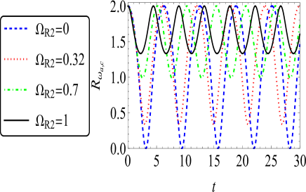
Figure 8: The dynamics of performance ratio $R_{{\textrm{$\omega$}}_{\mathrm{a,c}}}$, calculated for simultaneous estimation of $\omega_{a}$ and $\omega_{c}$, for ${\textrm{$\alpha$}},{\textrm{$\theta$}}{=}{\textrm{$\pi$}}{/}{2}$, $\Omega_{\mathrm{R1}}=1$ and different values of ${{\mathrm{\textrm{$\Omega$}}}}_{{R}{2}}$.

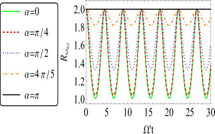
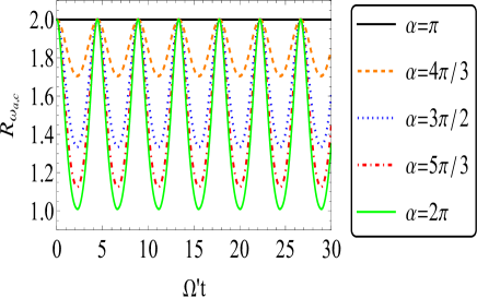
Figure 9: The variation of performance ratio $R_{{\textrm{$\omega$}}_{\mathrm{a,c}}}$, calculated for simultaneous estimation of $\omega_{a}$ and $\omega_{c}$, as a function of the scaled time $\Omega^{{}^{\prime}}t$ for $\theta$${=}{\textrm{$\pi$}}{/}{2}$ and different values of $\alpha$ in the equal Rabi frequencies regime.

.

In the second scenario we intend to estimate the two upper energy levels, i.e., $\{\omega_{a},\omega_{c}\}$. Here it is seen that the performance ratio $R_{\omega_{a,c}}$ may be enhanced by an increase in the Rabi frequency $\Omega_{\mathrm{R2}}$ (see Fig. 8). Hence, when the driving field coupling the upper ground and excited states is intensified considerably, the simultaneous strategy becomes advantageous than the individual one.

Again we find that in the equal Rabi frequencies regime if the coherent trapping occurs, $R_{\omega_{a,c}}$ is maximized, meaning complete superiority of the simultaneous estimation of the two upper energy levels compared to independent one (see Fig. 9).

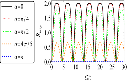
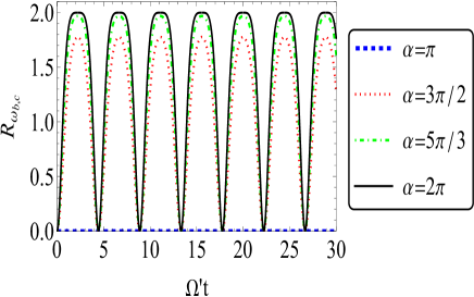
Figure 10: The variation of performance ratio $R_{{\textrm{$\omega$}}_{\mathrm{b,c}}}$, calculated for simultaneous estimation of $\omega_{b}$ and $\omega_{c}$, as a function of the scaled time $\Omega^{{}^{\prime}}t$ for $\theta$${=}{\textrm{$\pi$}}{/}{2}$ and different values of $\alpha$ in the equal Rabi frequencies regime.

.

V.2.3 Simultaneous estimation of $\omega_{b}$ and $\omega_{c}$

Interestingly, in the two previous subsections we saw that when the single upper level is simultaneously estimated with one of the lower levels, the best estimation is achieved provided that the coherent trapping occurs in the equal Rabi frequencies regime. Nevertheless, here we find that the simultaneous estimation of the lower levels completely fails when the population is trapped in those states, as shown in Fig. 10 in which $R_{\omega_{b,c}}$ is equal to zero in coherent trapping scenario.

However, if we can control the Rabi phases $(\phi_{1},\phi_{2})$ as well as the initial phase $\psi$ such that $\alpha=0$ is realized, the corresponding QFIM becomes diagonal at times ${\mathrm{\textrm{$\Omega$}}}^{\prime}t=\pi/\sqrt{2}$ for which the performance ratio $R_{\omega_{b,c}}$ is maximized, indicating completely supremacy of simultaneous estimation.

VI Conclusion and Discussion

Applying multi-level systems, or qudits, instead of qubits to implement quantum information tasks is a developing field promising advantages in some areas of quantum information. In particular, recent theoretical works suggest that quantum error correction with multi-level systems has potential advantages over qubit-based schemes. With these considerations, determining the energy levels of an atomic system is a crucial task to employ them in quantum information processing.

In this paper, considering a three-level atom interacting with laser fields, we examined the application of quantum metrology in atomic spectroscopy focusing on detection of spectra of atoms, ions, and sometimes molecular species based on measurements from both the electromagnetic and mass spectra. Computing the quantum Fisher information matrrix (QFIM), which is a key concept in quantum metrology, we investigated the effects of the initial preparation of the atom and the laser fields on energy levels estimation of the atom. It was shown that the influence of the laser phases on the quantum estimation can be controlled by the phase encoded into the initial state of the atom. Moreover, it was demonstrated that controlling the intensity of the laser fields, we can considerably enhance the estimation of the energy levels. In addition, the sensitive amplification enabled by coherent population trapping was discussed. Besides, we found that that there is a single measurement which is jointly optimal for extracting information on all energy levels, intending to estimate them simultaneously, ensuring the asymptotic saturability of the Cramer-Rao bound.

We have also constructed an important relationship for the three level system between the Hilbert–Schmidt speed (HSS), which is a special case of quantum statistical speed, and the QFI. It was shown that these two quantities, computed with respect to the same energy levels, exhibit the same qualitative dynamical behaviors. This relationship originates from the fact that the QFI is itself a quantum statistical speed associated with the Bures distance. Moreover, in contrast to the typical computational complication of the QFI, especially for high dimensional systems, the HSS is easily computable and hence it can be instead proposed as a powerful tool to estimate energy levels in three-level systems. Our results pave the way to further studies on applications of the HSS in quantum metrology as well as atomic spectroscopy.

Acknowledgments

H. R. J. wishes to acknowledge the financial support of the MSRT of Iran and Jahrom University *

Appendix A Analytical expressions of Quantum Fisher information in single estimation scenario

The QFIs associated with energy levels are given by:

$$F_{{\textrm{{\hbox{\omega}}}}_{\mathrm{a\ }}}=t^{2}\Bigg{(}1-{(-1+\frac{{\mathrm{sin}[\frac{1}{2}t\sqrt{{\textrm{{\hbox{\Omega}}}}^{2}_{\mathrm{R1}}+{\textrm{{\hbox{\Omega}}}}^{2}_{\mathrm{R2}}}]}^{2}({\textrm{{\hbox{\Omega}}}}^{2}_{\mathrm{R1}}+2\>\mathrm{cos}\textrm{{\hbox{\alpha}}}\>\mathrm{sin}\textrm{{\hbox{\theta}}}\>{\textrm{{\hbox{\Omega}}}}_{\mathrm{R1}}{\textrm{{\hbox{\Omega}}}}_{\mathrm{R2}}+{\textrm{{\hbox{\Omega}}}}^{2}_{\mathrm{R2}}+\mathrm{cos}\textrm{{\hbox{\theta}}}({\textrm{{\hbox{\Omega}}}}^{2}_{\mathrm{R1}}-{\textrm{{\hbox{\Omega}}}}^{2}_{\mathrm{R2}}))}{{\textrm{{\hbox{\Omega}}}}^{2}_{\mathrm{R1}}+{\textrm{{\hbox{\Omega}}}}^{2}_{\mathrm{R2}}})}^{2}\Bigg{)},$$ (29)

$$\begin{split}F_{{\textrm{$\omega$}}_{\mathrm{b\ }}}&=t^{2}\Bigg{(}1-\frac{1}{{({\textrm{$\Omega$}}^{2}_{\mathrm{R1}}+{\textrm{$\Omega$}}^{2}_{\mathrm{R2}})}^{4}}{({({\textrm{$\Omega$}}^{2}_{\mathrm{R1}}+{\textrm{$\Omega$}}^{2}_{\mathrm{R2}})}^{2}}\\ &+4\>\mathrm{cos}\textrm{$\alpha$}\>\mathrm{sin}\textrm{$\theta$}\>{\mathrm{sin}}^{2}[\frac{1}{4}t\sqrt{{\textrm{$\Omega$}}^{2}_{\mathrm{R1}}+{\textrm{$\Omega$}}^{2}_{\mathrm{R2}}}]{\textrm{$\Omega$}}_{\mathrm{R1}}{\textrm{$\Omega$}}_{\mathrm{R2}}(\mathrm{cos}[\frac{1}{2}t\sqrt{{\textrm{$\Omega$}}^{2}_{\mathrm{R1}}+{\textrm{$\Omega$}}^{2}_{\mathrm{R2}}}]{\textrm{$\Omega$}}^{2}_{\mathrm{R1}}+{\textrm{$\Omega$}}^{2}_{\mathrm{R2}})\\ &-({\textrm{$\Omega$}}^{2}_{\mathrm{R1}}+{\textrm{$\Omega$}}^{2}_{\mathrm{R2}})({\mathrm{cos}}^{2}[\frac{1}{2}t\sqrt{{\textrm{$\Omega$}}^{2}_{\mathrm{R1}}+{\textrm{$\Omega$}}^{2}_{\mathrm{R2}}}]{\textrm{$\Omega$}}^{2}_{\mathrm{R1}}+{\textrm{$\Omega$}}^{2}_{\mathrm{R2}})-\mathrm{cos}\textrm{$\theta$}((-1+4\>\mathrm{cos}[\frac{1}{2}t\sqrt{{\textrm{$\Omega$}}^{2}_{\mathrm{R1}}+{\textrm{$\Omega$}}^{2}_{\mathrm{R2}}}]){\textrm{$\Omega$}}^{2}_{\mathrm{R1}}{\textrm{$\Omega$}}^{2}_{\mathrm{R2}}\\ &+{\textrm{$\Omega$}}^{4}_{\mathrm{R2}}+{\mathrm{cos}}^{2}[\frac{1}{2}t\sqrt{{\mathrm{\textrm{$\Omega$}}^{2}_{\mathrm{R1}}}+{\textrm{$\Omega$}}^{2}_{\mathrm{R2}}}]({\textrm{$\Omega$}}^{4}_{\mathrm{R1}}-{\textrm{$\Omega$}}^{2}_{\mathrm{R1}}{\textrm{$\Omega$}}^{2}_{\mathrm{R2}})))^{2}\Bigg{)},\end{split}$$ (30)

$$\begin{split}F_{{\textrm{$\omega$}}_{\mathrm{c\ }}}&=t^{2}\Bigg{(}1-\frac{1}{{({\textrm{$\Omega$}}^{2}_{\mathrm{R1}}+{\textrm{$\Omega$}}^{2}_{\mathrm{R2}})}^{4}}{({({\textrm{$\Omega$}}^{2}_{\mathrm{R1}}+{\textrm{$\Omega$}}^{2}_{\mathrm{R2}})}^{2}+4\>\mathrm{cos}\textrm{$\alpha$}\>\mathrm{sin}\textrm{$\theta$}\>{\mathrm{sin}}^{2}[\frac{1}{4}t\sqrt{{\textrm{$\Omega$}}^{2}_{\mathrm{R1}}+{\textrm{$\Omega$}}^{2}_{\mathrm{R2}}}]{\textrm{$\Omega$}}_{\mathrm{R1}}{\textrm{$\Omega$}}_{\mathrm{R2}}({\textrm{$\Omega$}}^{2}_{\mathrm{R1}}}\\ &+\mathrm{cos}[\frac{1}{2}t\sqrt{{\textrm{$\Omega$}}^{2}_{\mathrm{R1}}+{\textrm{$\Omega$}}^{2}_{\mathrm{R2}}}]{\textrm{$\Omega$}}^{2}_{\mathrm{R2}})+(-{\textrm{$\Omega$}}^{2}_{\mathrm{R1}}-{\textrm{$\Omega$}}^{2}_{\mathrm{R2}})({\textrm{$\Omega$}}^{2}_{\mathrm{R1}}+{\mathrm{cos}}^{2}[\frac{1}{2}t\sqrt{{\textrm{$\Omega$}}^{2}_{\mathrm{R1}}+{\textrm{$\Omega$}}^{2}_{\mathrm{R2}}}]{\textrm{$\Omega$}}^{2}_{\mathrm{R2}})\\ &+\mathrm{cos}\textrm{$\theta$}(4\mathrm{cos}[\frac{1}{2}t\sqrt{{\textrm{$\Omega$}}^{2}_{\mathrm{R1}}+{\textrm{$\Omega$}}^{2}_{\mathrm{R2}}}]{\textrm{$\Omega$}}^{2}_{\mathrm{R1}}{\textrm{$\Omega$}}^{2}_{\mathrm{R2}}+({\textrm{$\Omega$}}^{2}_{\mathrm{R1}}-{\textrm{$\Omega$}}^{2}_{\mathrm{R2}})({\textrm{$\Omega$}}^{2}_{\mathrm{R1}}-{\mathrm{cos}}^{2}[\frac{1}{2}t\sqrt{{\textrm{$\Omega$}}^{2}_{\mathrm{R1}}+{\textrm{$\Omega$}}^{2}_{\mathrm{R2}}}]{\textrm{$\Omega$}}^{2}_{\mathrm{R2}})))^{2}\Bigg{)}.\end{split}$$ (31)

In the equal Rabi frequencies regime (${\mathrm{\textrm{$\Omega$}}}_{R1}=$ ${\mathrm{\textrm{$\Omega$}}}_{R2}$), the QFI expressions simplify as follows:

$$F_{{\textrm{{\hbox{\omega}}}}_{\mathrm{a\ }}}=-\frac{1}{2}t^{2}(1+\mathrm{cos}\textrm{{\hbox{\alpha}}}\>\mathrm{sin}\textrm{{\hbox{\theta}}}){\mathrm{sin}[\frac{t{\textrm{{\hbox{\Omega}}}^{\prime}}}{\sqrt{2}}]}^{2}\left(-3-\mathrm{cos}[\sqrt{2}t{\textrm{{\hbox{\Omega}}}^{\prime}}]+2\>\mathrm{cos}\textrm{{\hbox{\alpha}}}\>\mathrm{sin}\textrm{{\hbox{\theta}}}\>{\mathrm{sin}[\frac{t{\textrm{{\hbox{\Omega}}}}^{\prime}}{\sqrt{2}}]}^{2}\right),$$ (32)

$$\begin{split}F_{{\textrm{$\omega$}}_{\mathrm{b\ }}}&=\frac{1}{128}\>t^{2}\Bigg{(}81-\mathrm{cos}[2\textrm{$\theta$}](29+36\>\mathrm{cos}[\sqrt{2}\>t{\textrm{$\Omega$}^{\prime}}])-4\>\mathrm{cos}[2\sqrt{2}\>t{\textrm{$\Omega$}^{\prime}}]{(1+\mathrm{cos}\textrm{$\alpha$}\>\mathrm{sin}\textrm{$\theta$})}^{2}\\ &-6\>\mathrm{sin}\textrm{$\theta$}(4\>\mathrm{cos}\textrm{$\alpha$}+\mathrm{cos}[2\textrm{$\alpha$}]\>\mathrm{sin}\textrm{$\theta$})+4\>\mathrm{cos}[\sqrt{2}\>t{\textrm{$\Omega$}^{\prime}}](-3+8\>\mathrm{cos}\textrm{$\alpha$}\>\mathrm{sin}\textrm{$\theta$}+2\>\mathrm{cos}[2\textrm{$\alpha$}]\>{\mathrm{sin}\textrm{$\theta$}}^{2})\\ &+128\>\mathrm{cos}\textrm{$\theta$}\>\mathrm{cos}[\frac{t{\textrm{$\Omega$}^{\prime}}}{\sqrt{2}}](1+\mathrm{cos}\textrm{$\alpha$}\>\mathrm{sin}\textrm{$\theta$}){\mathrm{sin}[\frac{t{\textrm{$\Omega$}^{\prime}}}{\sqrt{2}}]}^{2}\Bigg{)},\end{split}$$ (33)

$$\begin{split}F_{{\textrm{$\omega$}}_{\mathrm{c\ }}}&=\frac{1}{128}\>t^{2}\Bigg{(}81-\mathrm{cos}[2\textrm{$\theta$}](29+36\>\mathrm{cos}[\sqrt{2}\>t{\textrm{$\Omega$}^{\prime}}])-4\>\mathrm{cos}[2\sqrt{2}\>t{\textrm{$\Omega$}^{\prime}}]{(1+\mathrm{cos}\textrm{$\alpha$}\>\mathrm{sin}\textrm{$\theta$})}^{2}\\ &-6\>\mathrm{sin}\textrm{$\theta$}(4\>\mathrm{cos}\textrm{$\alpha$}+\mathrm{cos}[2\textrm{$\alpha$}]\>\mathrm{sin}\textrm{$\theta$})+4\>\mathrm{cos}[\sqrt{2}\>t{\textrm{$\Omega$}^{\prime}}](-3+8\>\mathrm{cos}\textrm{$\alpha$}\>\mathrm{sin}\textrm{$\theta$}+2\>\mathrm{cos}[2\textrm{$\alpha$}]\>{\mathrm{sin}\textrm{$\theta$}}^{2})\\ &-128\>\mathrm{cos}\textrm{$\theta$}\>\mathrm{cos}[\frac{t{\textrm{$\Omega$}^{\prime}}}{\sqrt{2}}](1+\mathrm{cos}\textrm{$\alpha$}\>\mathrm{sin}\textrm{$\theta$}){\mathrm{sin}[\frac{t{\textrm{$\Omega$}^{\prime}}}{\sqrt{2}}]}^{2}\Bigg{)}.\end{split}$$ (34)

References

- Helstrom [1976] C. W. Helstrom, Quantum detection and estimation theory, Vol. 3 (Academic Press, New York, 1976).
- Holevo [2011] A. S. Holevo, Probabilistic and statistical aspects of quantum theory, Vol. 1 (Springer Science & Business Media, 2011).
- Lu and Wang [2021] X.-M. Lu and X. Wang, Incorporating heisenberg’s uncertainty principle into quantum multiparameter estimation, Phys. Rev. Lett. 126, 120503 (2021).
- Fiderer et al. [2021] L. J. Fiderer, T. Tufarelli, S. Piano, and G. Adesso, General expressions for the quantum fisher information matrix with applications to discrete quantum imaging, PRX Quantum 2, 020308 (2021).
- Rangani Jahromi [2019] H. Rangani Jahromi, Weak measurement effect on optimal estimation with lower and upper bound on relativistic metrology, Int. J. Mod. Phys. D 28, 1950162 (2019).
- Farajollahi et al. [2018] B. Farajollahi, M. Jafarzadeh, H. R. Jahromi, and M. Amniat-Talab, Estimation of temperature in micromaser-type systems, Quantum Inf. Process 17, 1 (2018).
- Jahromi [2020] H. R. Jahromi, Quantum thermometry in a squeezed thermal bath, Phys. Scr 95, 035107 (2020).
- Jafarzadeh et al. [2020] M. Jafarzadeh, H. Rangani Jahromi, and M. Amniat-Talab, Effects of partial measurements on quantum resources and quantum fisher information of a teleported state in a relativistic scenario, Proc. R. Soc. A 476, 20200378 (2020).
- Braunstein [1992] S. L. Braunstein, Quantum limits on precision measurements of phase, Phys. Rev. Lett. 69, 3598 (1992).
- Braunstein and Caves [1994a] S. L. Braunstein and C. M. Caves, Statistical distance and the geometry of quantum states, Phys. Rev. Lett. 72, 3439 (1994a).
- Lee et al. [2002] H. Lee, P. Kok, and J. P. Dowling, A quantum rosetta stone for interferometry, J. Mod. Opt 49, 2325 (2002).
- Giovannetti et al. [2004] V. Giovannetti, S. Lloyd, and L. Maccone, Quantum-enhanced measurements: beating the standard quantum limit, Science 306, 1330 (2004).
- Giovannetti et al. [2006] V. Giovannetti, S. Lloyd, and L. Maccone, Quantum metrology, Phys. Rev. Lett. 96, 010401 (2006).
- Giovannetti et al. [2011] V. Giovannetti, S. Lloyd, and L. Maccone, Advances in quantum metrology, Nat. Photonics 5, 222 (2011).
- Paris [2009] M. G. Paris, Quantum estimation for quantum technology, Int. J. Quantum Inf. 7, 125 (2009).
- Jahromi and Amniat-Talab [2015] H. R. Jahromi and M. Amniat-Talab, Geometric phase, entanglement, and quantum fisher information near the saturation point, Ann. Phys. (N. Y.) 355, 299 (2015).
- Jahromi [2018] H. R. Jahromi, Parameter estimation in plasmonic qed, Opt. Commun 411, 119 (2018).
- Polino et al. [2020] E. Polino, M. Valeri, N. Spagnolo, and F. Sciarrino, Photonic quantum metrology, AVS Quantum Sci 2, 024703 (2020).
- Sidhu and Kok [2020] J. S. Sidhu and P. Kok, Geometric perspective on quantum parameter estimation, AVS Quantum Sci 2, 014701 (2020).
- Gianani et al. [2020] I. Gianani, M. G. Genoni, and M. Barbieri, Assessing data postprocessing for quantum estimation, IEEE J. Sel. Top. Quantum Electron 26, 1 (2020).
- Jahromi [2021] H. R. Jahromi, Remote magnetic sensing and faithful quantum teleportation through non-localized qubits, arXiv preprint arXiv:2109.05275 (2021).
- Tóth and Apellaniz [2014] G. Tóth and I. Apellaniz, Quantum metrology from a quantum information science perspective, J PHYS A-MATH THEOR. 47, 424006 (2014).
- Demkowicz-Dobrzański et al. [2015] R. Demkowicz-Dobrzański, M. Jarzyna, and J. Kołodyński, Quantum limits in optical interferometry, Prog. Opt. 60, 345 (2015).
- Moreau et al. [2019] P.-A. Moreau, E. Toninelli, T. Gregory, and M. J. Padgett, Imaging with quantum states of light, Nat. Rev. Phys. 1, 367 (2019).
- Xu et al. [2019] C. Xu, L. Zhang, S. Huang, T. Ma, F. Liu, H. Yonezawa, Y. Zhang, and M. Xiao, Sensing and tracking enhanced by quantum squeezing, Photonics Res. 7, A14 (2019).
- Pirandola et al. [2018] S. Pirandola, B. R. Bardhan, T. Gehring, C. Weedbrook, and S. Lloyd, Advances in photonic quantum sensing, Nat. Photonics 12, 724 (2018).
- Genovese [2016] M. Genovese, Real applications of quantum imaging, J. Opt 18, 073002 (2016).
- Albarelli et al. [2020] F. Albarelli, M. Barbieri, M. G. Genoni, and I. Gianani, A perspective on multiparameter quantum metrology: From theoretical tools to applications in quantum imaging, Phys. Lett. A 384, 126311 (2020).
- Demkowicz-Dobrzański et al. [2020] R. Demkowicz-Dobrzański, W. Górecki, and M. Guţă, Multi-parameter estimation beyond quantum fisher information, J. Phys. A 53, 363001 (2020).
- Szczykulska et al. [2016] M. Szczykulska, T. Baumgratz, and A. Datta, Multi-parameter quantum metrology, Adv. Phys.: X 1, 621 (2016).
- Jahromi et al. [2019] H. R. Jahromi, M. Amini, and M. Ghanaatian, Multiparameter estimation, lower bound on quantum fisher information, and non-markovianity witnesses of noisy two-qubit systems, Quantum Inf. Process 18, 1 (2019).
- Pezze et al. [2018] L. Pezze, A. Smerzi, M. K. Oberthaler, R. Schmied, and P. Treutlein, Quantum metrology with nonclassical states of atomic ensembles, Rev. Mod. Phys 90, 035005 (2018).
- Degen et al. [2017] C. L. Degen, F. Reinhard, and P. Cappellaro, Quantum sensing, Rev. Mod. Phys 89, 035002 (2017).
- Schirhagl et al. [2014] R. Schirhagl, K. Chang, M. Loretz, and C. L. Degen, Nitrogen-vacancy centers in diamond: nanoscale sensors for physics and biology, Annu. Rev. Phys. Chem 65, 83 (2014).
- Proctor et al. [2018] T. J. Proctor, P. A. Knott, and J. A. Dunningham, Multiparameter estimation in networked quantum sensors, Phys. Rev. Lett. 120, 080501 (2018).
- Qian et al. [2019] K. Qian, Z. Eldredge, W. Ge, G. Pagano, C. Monroe, J. V. Porto, and A. V. Gorshkov, Heisenberg-scaling measurement protocol for analytic functions with quantum sensor networks, Phys. Rev. A 100, 042304 (2019).
- Sekatski et al. [2020] P. Sekatski, S. Wölk, and W. Dür, Optimal distributed sensing in noisy environments, Phys. Rev. Research 2, 023052 (2020).
- Guo et al. [2020] X. Guo, C. R. Breum, J. Borregaard, S. Izumi, M. V. Larsen, T. Gehring, M. Christandl, J. S. Neergaard-Nielsen, and U. L. Andersen, Distributed quantum sensing in a continuous-variable entangled network, Nat. Phys. 16, 281 (2020).
- Xia et al. [2020] Y. Xia, W. Li, W. Clark, D. Hart, Q. Zhuang, and Z. Zhang, Demonstration of a reconfigurable entangled radio-frequency photonic sensor network, Phys. Rev. Lett. 124, 150502 (2020).
- Baumgratz and Datta [2016] T. Baumgratz and A. Datta, Quantum enhanced estimation of a multidimensional field, Phys. Rev. Lett. 116, 030801 (2016).
- Apellaniz et al. [2018] I. Apellaniz, I. Urizar-Lanz, Z. Zimborás, P. Hyllus, and G. Tóth, Precision bounds for gradient magnetometry with atomic ensembles, Phys. Rev. A 97, 053603 (2018).
- DeVience et al. [2015] S. J. DeVience, L. M. Pham, I. Lovchinsky, A. O. Sushkov, N. Bar-Gill, C. Belthangady, F. Casola, M. Corbett, H. Zhang, M. Lukin, et al., Nanoscale nmr spectroscopy and imaging of multiple nuclear species, Nat. Nanotechnol. 10, 129 (2015).
- Komar et al. [2014] P. Komar, E. M. Kessler, M. Bishof, L. Jiang, A. S. Sørensen, J. Ye, and M. D. Lukin, A quantum network of clocks, Nat. Phys 10, 582 (2014).
- Khabiboulline et al. [2019] E. T. Khabiboulline, J. Borregaard, K. De Greve, and M. D. Lukin, Optical interferometry with quantum networks, Phys. Rev. Lett. 123, 070504 (2019).
- Scully et al. [1997] M. O. Scully, M. S. Zubairy, et al., Quantum optics cambridge university press, Cambridge, CB2 2RU, UK (1997).
- Lin et al. [1993] H. Lin, J. Gubernatis, H. Gould, and J. Tobochnik, Exact diagonalization methods for quantum systems, Comput. Phys. Commun 7, 400 (1993).
- Jones et al. [2019] T. Jones, S. Endo, S. McArdle, X. Yuan, and S. C. Benjamin, Variational quantum algorithms for discovering hamiltonian spectra, Phys. Rev. A 99, 062304 (2019).
- De Vivo et al. [2016] M. De Vivo, M. Masetti, G. Bottegoni, and A. Cavalli, Role of molecular dynamics and related methods in drug discovery, J. Med. Chem. 59, 4035 (2016).
- Reiher et al. [2017] M. Reiher, N. Wiebe, K. M. Svore, D. Wecker, and M. Troyer, Elucidating reaction mechanisms on quantum computers, Proc. Natl. Acad. Sci. U.S.A 114, 7555 (2017).
- Brida et al. [2011] G. Brida, I. P. Degiovanni, A. Florio, M. Genovese, P. Giorda, A. Meda, M. G. Paris, and A. P. Shurupov, Optimal estimation of entanglement in optical qubit systems, Phys. Rev. A 83, 052301 (2011).
- Ciampini et al. [2016] M. A. Ciampini, N. Spagnolo, C. Vitelli, L. Pezzè, A. Smerzi, and F. Sciarrino, Quantum-enhanced multiparameter estimation in multiarm interferometers, Sci. Rep. 6, 1 (2016).
- Yousefjani et al. [2017] R. Yousefjani, R. Nichols, S. Salimi, and G. Adesso, Estimating phase with a random generator: Strategies and resources in multiparameter quantum metrology, Physical Review A 95, 062307 (2017).
- Humphreys et al. [2013] P. C. Humphreys, M. Barbieri, A. Datta, and I. A. Walmsley, Quantum enhanced multiple phase estimation, Phys. Rev. Lett. 111, 070403 (2013).
- Liu et al. [2019] J. Liu, H. Yuan, X.-M. Lu, and X. Wang, Quantum fisher information matrix and multiparameter estimation, J. Phys. A Math. Theor. 53, 023001 (2019).
- Ivanov and Vitanov [2018] P. A. Ivanov and N. V. Vitanov, Quantum sensing of the phase-space-displacement parameters using a single trapped ion, Phys. Rev. A. 97, 032308 (2018).
- Braunstein and Caves [1994b] S. L. Braunstein and C. M. Caves, Statistical distance and the geometry of quantum states, Phys. Rev. Lett. 72, 3439 (1994b).
- Ragy et al. [2016] S. Ragy, M. Jarzyna, and R. Demkowicz-Dobrzański, Compatibility in multiparameter quantum metrology, Phys. Rev. A 94, 052108 (2016).
- Napoli et al. [2019] C. Napoli, S. Piano, R. Leach, G. Adesso, and T. Tufarelli, Towards superresolution surface metrology: quantum estimation of angular and axial separations, Phys. Rev. Lett. 122, 140505 (2019).
- Vanier [2005] J. Vanier, Atomic clocks based on coherent population trapping: a review, Appl. Phys. B 81, 421 (2005).
- Shah and Kitching [2010] V. Shah and J. Kitching, Advances in coherent population trapping for atomic clocks, Adv. At. Mol. 59, 21 (2010).
- Zhu and Cutler [2000] M. Zhu and L. Cutler, Theoretical and experimental study of light shift in a cpt-based rb vapor cell frequency standard, in Proceedings of the 32th Annual Precise Time and Time Interval Systems and Applications Meeting (2000) pp. 311–324.
- Liu et al. [2017] X. Liu, E. Ivanov, V. I. Yudin, J. Kitching, and E. A. Donley, Low-drift coherent population trapping clock based on laser-cooled atoms and high-coherence excitation fields, Phys. Rev. Appl. 8, 054001 (2017).
- Schwindt et al. [2004] P. D. Schwindt, S. Knappe, V. Shah, L. Hollberg, J. Kitching, L.-A. Liew, and J. Moreland, Chip-scale atomic magnetometer, Appl. Phys. Lett. 85, 6409 (2004).
- Liu et al. [2013] X. Liu, J.-M. Merolla, S. Guérandel, E. De Clercq, and R. Boudot, Ramsey spectroscopy of high-contrast cpt resonances with push-pull optical pumping in cs vapor, Opt. Express 21, 12451 (2013).
- Cheng et al. [2016] B. Cheng, P. Gillot, S. Merlet, and F. P. Dos Santos, Coherent population trapping in a raman atom interferometer, Phys. Rev. A 93, 063621 (2016).
- Neveu et al. [2018] P. Neveu, C. Banerjee, J. Lugani, F. Bretenaker, E. Brion, and F. Goldfarb, Phase sensitive amplification enabled by coherent population trapping, New J. Phys. 20, 083043 (2018).
- Gessner and Smerzi [2018] M. Gessner and A. Smerzi, Statistical speed of quantum states: Generalized quantum Fisher information and Schatten speed, Phys. Rev. A 97, 022109 (2018).
- Jahromi et al. [2020] H. R. Jahromi, K. Mahdavipour, M. K. Shadfar, and R. L. Franco, Witnessing non-markovian effects of quantum processes through hilbert-schmidt speed, Phys. Rev. A 102, 022221 (2020).
- Rangani Jahromi and Lo Franco [2021] H. Rangani Jahromi and R. Lo Franco, Hilbert–schmidt speed as an efficient figure of merit for quantum estimation of phase encoded into the initial state of open n-qubit systems, Sci. Rep. 11, 1 (2021).