Operator-induced structural variable selection for identifying materials genes

Abstract

In the emerging field of materials informatics, a fundamental task is to identify physicochemically meaningful descriptors, or materials genes, which are engineered from primary features and a set of elementary algebraic operators through compositions. Standard practice directly analyzes the high-dimensional candidate predictor space in a linear model; statistical analyses are then substantially hampered by the daunting challenge posed by the astronomically large number of correlated predictors with limited sample size. We formulate this problem as variable selection with operator-induced structure (OIS) and propose a new method to achieve unconventional dimension reduction by utilizing the geometry embedded in OIS. Although the model remains linear, we iterate nonparametric variable selection for effective dimension reduction. This enables variable selection based on ab initio primary features, leading to a method that is orders of magnitude faster than existing methods, with improved accuracy. To select the nonparametric module, we discuss a desired performance criterion that is uniquely induced by variable selection with OIS; in particular, we propose to employ a Bayesian Additive Regression Trees (BART)-based variable selection method. Numerical studies show superiority of the proposed method, which continues to exhibit robust performance when the input dimension is out of reach of existing methods. Our analysis of single-atom catalysis identifies physical descriptors that explain the binding energy of metal-support pairs with high explanatory power, leading to interpretable insights to guide the prevention of a notorious problem called sintering and aid catalysis design.

Keywords: BART; Bayesian nonparametrics; feature engineering; materials genomes; nonparametric dimension reduction

1 Introduction

The Materials Genome Initiative set up by the White House is a large-scale effort concerning the utilization of computational tools to accelerate the pace of discovery and deployment of advanced material systems. Since its inception in 2011, there has been a surge of interest in data-driven materials design and understanding (Zhong et al., 2020; Hart et al., 2021; Keith et al., 2021; Lin et al., 2021; Liu et al., 2021a). In this nascent area called materials informatics, computational methods that account for physical and chemical mechanisms of a material system play a central role in aiding, augmenting, or even replacing the time-consuming trial and error experimentation. A fundamental task is to identify physicochemically meaningful descriptors, or materials genes (Ghiringhelli et al., 2015; Foppa et al., 2021). These descriptors, for example, are key to modeling single-atom catalysis and finding or developing more efficient catalytically active materials. In statistical terms, descriptors are high-dimensional predictors but with strong structure in that they are functional transformations of a set of primary features $\bm{X}=(\bm{x}_{1},\ldots,\bm{x}_{p})$. For instance, a simple example of descriptors is $f(\bm{X})=\{\exp(\bm{x}_{1})-\exp(\bm{x}_{2})\}^{2}$, which can be constructed using exponential and squared functions in combination with subtraction.

Suppose the response vector $\bm{y}$ measures the material property of interest, and the primary features matrix $\bm{X}=(\bm{x}_{1},\ldots,\bm{x}_{p})$ collects physical or chemical properties of the materials such as atomic radii, ionization energies, etc. Then the space of engineered predictors (or descriptors) up to order $M$ is $\mathcal{O}^{(M)}(\bm{X})$, which consists of nonlinear predictors with explicit functional form resulting from $M$-order compositions of operators $\mathcal{O}$ on $\bm{X}$:

$$\mathcal{O}^{(M)}(\bm{X})=\mathcal{O}\circ\mathcal{O}^{(M-1)}(\bm{X})=\underbrace{\mathcal{O}\circ\cdots\circ\mathcal{O}}_{M\text{ times}}(\bm{X}).$$ (1)

For example, some commonly used operators in materials genome are

$$\mathcal{O}=\{+,-,\times,/,|-|,I,\exp,\log,|\cdot|,\sqrt{},^{-1},^{2},\sin(\pi\cdot),\cos(\pi\cdot)\},$$ (2)

and the aforementioned descriptor $f(\bm{X})=\{\exp(\bm{x}_{1})-\exp(\bm{x}_{2})\}^{2}$ belongs to $\mathcal{O}^{(3)}(\bm{X})$. We refer to this distinctive geometry encoded in $\mathcal{O}^{(M)}(\bm{X})$ as operator-induced structure (OIS). The aforementioned descriptors in materials genome are thus the predictors in a linear model with OIS. Henceforth, we will use descriptor selection and variable selection in the presence of OIS interchangeably. Note that the specification of $\mathcal{O}$ depends on domain knowledge, and we intentionally include the absolute difference operator $|-|$ in $\mathcal{O}$ because it is directly interpretable in materials science, and it often provides clear intuition on many physical phenomena, such as the metal-oxide binding energy (Liu et al., 2022). Treating it as a single operator reduces the required number of iterations to generate related descriptors.

A common practice in materials genome (O’Connor et al., 2018; Ouyang et al., 2018; Liu et al., 2020) is to employ modern statistical variable selection developed for linear models. However, the geometry of OIS defined by operators $\mathcal{O}$ and high-order compositions induces high correlation and ultra-high dimension to the feature space. As detailed in Section 2, the dimension of $\mathcal{O}^{(M)}(\bm{X})$ increases double exponentially with $M$ and the number of binary operators in $\mathcal{O}$. For example, with $p=59$ in our real data application, enumerating $\mathcal{O}^{(3)}(\bm{X})$ gives $1.01\times 10^{17}$ predictors while only a handful of them are associated with the response. Moreover, these predictors are highly correlated as a result of iteratively applying unary operators. This along with a small size such as $n=91$ in our real data application substantially hurdles the performance of existing methods that rely on linear variable selection methods. Indeed, materials genomes are an analog concept to genomes, but the dimension of predictors and inherent strong correlation in materials genome-wide association studies, or materials GWAS, pose unprecedented challenges to statistical analysis.

In this article, we aim to develop a powerful method for materials GWAS in which we effectively identify materials genes that are associated with the response of interest. To achieve dimension reduction in materials GWAS, we consider an iterative approach by applying a small set of operators and immediately identifying the relevant descriptors, $\mathcal{D}$, before constructing more complex descriptors. This step is iterated in light of the composition structure in OIS, in striking contrast to existing literature that aims to exhaustively generate $\mathcal{O}^{(M)}(\bm{X})$. In each iteration, $\mathcal{O}(\mathcal{D})$ is typically substantially smaller than $\mathcal{O}^{(M)}(\bm{X})$, and such sparsity achieves dimension reduction and tackles the daunting computational challenges posed by materials GWAS.

Iterative dimension reduction, however, faces two intertwined challenges. First, the constructed descriptors in intermediate steps, unlike the astronomically large $\mathcal{O}^{(M)}(\bm{X})$, are not necessarily linearly associated with the response. To address this, we propose to use nonparametric variable selection for dimension reduction to ensure selection accuracy under the geometry of OIS. That is, while the model is assumed to be linear, we employ nonparametric variable selection to achieve dimension reduction while maintaining high selection accuracy. We refer to this key novelty of our proposed method as “parametrics assisted by nonparametrics”, or PAN.

The second challenge pertains to the selection of the nonparametric module. Unlike traditional nonparametric variable selection, OIS variable selection calls for new performance criteria for the nonparametric module to ensure OIS selection accuracy (see Section 2.3 for more details). We introduce a PAN criterion to reassess nonparametric selection methods, which elucidates an asymmetric effect between false positives and false negatives and highlights a desired invariance property to unary transformations. In particular, we propose to use a Bayesian additive regression tree variable selection method, BART-G.SE (Bleich et al., 2014), as the nonparametric module, which we show is well suited to satisfy the PAN criterion.

Coupling the PAN strategy with BART-G.SE, together with additional considerations to address the complexities of materials GWAS, leads to a new method for materials GWAS, which we call iterative BART, or iBART. The iterative framework of iBART reduces the size of the effective descriptor space significantly, mitigating collinearity in the process, and the use of nonparametric variable selection accounts for structural model misspecification in intermediate variable selection steps. Our extensive experiments show that iBART gives excellent performance with accuracy and scalability that are not seen in existing methods. Note that iBART is not a new BART variant for nonparametric regression, but rather an iterative use of BART within the PAN framework specifically tailored for materials GWAS.

The outline of the article is as follows. Section 1.1 reviews related work in materials genome. In Section 2, we introduce the OIS framework, describe the PAN selection procedure, and discuss how to choose the nonparametric module in PAN and some practical considerations regarding PAN. Section 3 contains a simulation study that shows superior performance of iBART relative to existing methods. In Section 4, we apply iBART to a single-atom catalysis data set and it identifies physical descriptors that explain the binding energy of metal-support pairs with high explanatory power, leading to interpretable insights to guide the prevention of a notorious problem called sintering. We close in Section 5 with a discussion. All proofs, details of variants of iBART, and additional simulation results and discussion are deferred to the Supplementary Material.

1.1 Related work

Descriptor selection has attracted growing attention in materials science. Recent methods often build on a one-shot descriptor generation and selection scheme followed by modern statistical variable selection approaches (O’Connor et al., 2018; Ouyang et al., 2018; Liu et al., 2020). In particular, they first construct descriptors by applying operators iteratively $M$ times on the primary feature space $\bm{X}^{(0)}\equiv\bm{X}=(\bm{x}_{1},\ldots,\bm{x}_{p})\in\mathbb{R}^{n\times p}$ to construct an ultra-high dimensional descriptor space $\bm{X}^{(M)}\equiv\mathcal{O}^{(M)}(\bm{X})$ of $O(p^{2^{M}})$ descriptors, assuming binary operators are used in each iteration. Then variants of generic statistical methods are adopted to select variables from $\bm{X}^{(M)}$. Along this line, the method SISSO (Sure Independence Screening and Sparsifying Operator) proposed by Ouyang et al. (2018) builds on Sure Independence Screening, or SIS (Fan and Lv, 2008), O’Connor et al. (2018) uses LASSO (Tibshirani, 1996), and Liu et al. (2020) adopts Bayesian variable selection methods.

SISSO is widely perceived as one of the most popular methods for materials genome. It utilizes SIS to screen out $P$ descriptors, from which the single best descriptor is selected using an $\ell_{0}$-penalized regression. If a total of $k$ descriptors are desired, this process will be iterated for $k$ times yielding $k$ sets of SIS-selected descriptors, followed by an $\ell_{0}$-penalized regression to select the best $k$ descriptors from all the SIS-selected descriptors. Note that in each iteration, SIS is employed to screen out $P$ descriptors from the remaining descriptor set with an updated response vector given by its least squares residuals projected onto the space spanned by previously SIS-selected descriptors. Users must define the composition complexity of the descriptors through $M$, i.e., the order of compositions of operators. In a typical application of SISSO, the composition complexity $M$ is no greater than 3, the number of candidate descriptors in each SIS iteration is less than 100, and the number of descriptors $k$ is no larger than 5 (Ouyang et al., 2018). Note that selecting 5 descriptors with 100 SIS-selected descriptors in each iteration amounts to fitting at most $\binom{500}{5}\approx 2.6\times 10^{11}$ different regressions, which is computationally intensive.

A major drawback of these one-shot descriptor construction procedures is the introduction of a highly correlated and ultra-high dimensional descriptor space $\bm{X}^{(M)}$. High correlation often hampers the performance of a variable selection method, and the ultra-high dimensional descriptor space with large $p$, as common in modern applications, can make it computationally prohibitive for such methods. In practice, these methods often resort to ad hoc adaptation or sacrifice the complexity level of candidate descriptors.

Another thread of work is the well-developed automatic feature engineering in machine learning, aiming to generate complex features from given constructor functions adaptively (Markovitch and Rosenstein, 2002; Feurer et al., 2015; Khurana et al., 2018). However, the overwhelming focus of this literature is on increasing the predictive power of the primary features $\bm{X}$. We instead focus on discovering the underlying functional relationship between the response and the predictors and revealing data-driven insights into the underlying physics of materials design. In addition, the sample size in materials genome is typically limited, hampering the use of machine learning methods that rely on large training data.

In statistics, transformations have been commonly used to expand the predictor space, including polynomials, logarithmic, power transformations, and the previously noted interactions. The induced feature spaces from these elementary transformations are often overly simple to capture the intricate dynamics of the response in materials genome, particularly compared to high-order compositions of a larger operator set. There has been a rich literature on nonparametric variable selection, but descriptor selection relies on a linear model with feature engineering that favorably points to interpretable insights for domain experts as the functional forms of selected variables are explicitly given and the feature space could be composed using domain-related knowledge. The nonparametric module in PAN only serves as a dimension reduction tool, and the desired performance calls for new investigation under the context of OIS. Overall, materials GWAS may play an analogous role that GWAS have played in motivating new statistical methods and concepts, and to the best of our knowledge, the present article is the first statistical work on this topic.

2 The OIS framework

2.1 Operator-induced structural model

We begin with a standard ultra-high dimensional linear regression model

$$\bm{y}=\beta_{0}+\beta_{1}\bm{x}_{1}+\cdots+\beta_{p^{\star}}\bm{x}_{p^{\star}}+\bm{\varepsilon},$$ (3)

where $\bm{\varepsilon}\sim\mathcal{N}_{n}(\bm{0},\sigma^{2}\bm{I})$ is a Gaussian noise vector, and the regression coefficients $\bm{\beta}$ are sparse. The dimension of predictors $p^{\star}$ is ultra-high, at the materials GWAS scale that typically exceeds the maximum size of matrices allowed by a modern personal computer, while the sample size $n$ is on the order of tens. In this paper, we assume that this seemingly ultra-dimensional descriptor space obeys an operator-induced structure (OIS). In particular, we assume that the predictors $\bm{x}_{1},\ldots,\bm{x}_{p^{\star}}$ in (3), or descriptors, are generated by applying operators in $\mathcal{O}$ iteratively $M$ times on a primary feature space $\bm{X}=(\bm{x}_{1},\ldots,\bm{x}_{p})\in\mathbb{R}^{n\times p}$,

$$(\bm{x}_{1},\ldots,\bm{x}_{p^{\star}})\equiv\bm{X}^{(M)}=\mathcal{O}^{(M)}(\bm{X})=\mathcal{O}\circ\mathcal{O}^{(M-1)}(\bm{X})=\underbrace{\mathcal{O}\circ\cdots\circ\mathcal{O}}_{M\text{ times}}(\bm{X}),$$ (4)

where $\bm{X}^{(M)}=\mathcal{O}^{(M)}(\bm{X})$ denotes $M$-composition of $\mathcal{O}$ on $\bm{X}$ and can be defined iteratively as above. The operator set $\mathcal{O}$ is user-defined; for concreteness, we focus on the common example given in (2), unless stated otherwise.

We adopt the following convention. Evaluation of operators on vectors is defined to be entry-wise, e.g., $\bm{x}^{2}_{1}=(x_{1,1}^{2},\ldots,x_{n,1}^{2})^{T}$ and $\bm{x}_{1}+\bm{x}_{2}=(x_{1,1}+x_{1,2},\ldots,x_{n,1}+x_{n,2})^{T}$. Throughout this article, we assume that all descriptors in $\bm{X}^{(M)}$ are uniquely defined in terms of their numerical values. For instance, only one of the descriptors in $\{\bm{x}_{1}^{2},\bm{x}_{1}\times\bm{x}_{1}\}$ will be kept in $\bm{X}^{(M)}$. This can be easily achieved in practice by identifying and removing perfectly correlated descriptors.

We hereafter refer to the linear regression model in (3) along with the operator-induced structure (OIS) in (4) as the OIS model. To facilitate a precise OIS model definition using predictors with nonzero coefficients, we define $M$-composition descriptor as follows.

Definition 2.1 ($M$-composition descriptor).

We define $f^{(M)}(\bm{X})$ to be an $M$-composition descriptor if it is constructed via $M$ compositions of operators on some primary features $\bm{X}$: $f^{(M)}(\bm{X})=o^{(M)}(\bm{X})=o_{M}\circ f^{(M-1)}(\bm{X})=o_{M}\circ o_{M-1}\circ\cdots\circ o_{1}(\bm{X}),$ where $o_{m}\in\mathcal{O}$ is the $m$-th composition operator(s) for $1\leq m\leq M$, and $f^{(1)}(\bm{X}),\ldots,f^{(M-1)}(\bm{X})$ are the necessary intermediate descriptors for constructing the descriptor $f^{(M)}(\bm{X})$.

Note that if the $m$-th composition operator is a binary operator, there may exist two $(m-1)$-th composition operators but we suppress the notation in the definition above for simplicity. Furthermore, if an $M$-composition descriptor $f^{(M)}(\bm{X})$ only depends on a subset of primary features $\bm{X}_{\mathcal{S}}$, where $\mathcal{S}\subseteq[p]=\{1,\ldots,p\}$, we also write it as $f^{(M)}(\bm{X}_{\mathcal{S}})$ and call it an $(M,\mathcal{S})$-descriptor.

Definition 2.2 ($(M,\mathcal{S})$-composition OIS model).

An $(M,\mathcal{S})$-OIS model assumes

$$\bm{y}=\beta_{0}+\sum_{k=1}^{K}f_{k}^{(M_{k})}(\bm{X}_{\mathcal{S}_{k}})\beta_{k}+\bm{\varepsilon},$$ (5)

where $M=\max_{k=1,\ldots,K}M_{k}$ denotes the highest order of operator compositions, $K$ denotes the number of additive descriptors, $\bm{X}_{\mathcal{S}_{k}}$ is the set of primary features used in the $k$-th descriptors, and $\mathcal{S}=\bigcup_{k=1}^{K}\mathcal{S}_{k}$ is the set of all active primary feature indices.

Throughout the article, we assume the data follows an $(M,\mathcal{S})$-OIS model in (5). We use $M_{0}$ for the oracle highest composition complexity and $\mathcal{S}_{0}$ for the oracle set of active primary feature indices. Descriptors in the $(M,\mathcal{S})$-OIS model and their intermediate descriptors are called active. We next use a toy example to illustrate the introduced concepts in OIS and the challenges posed by descriptor selection. Suppose that the data-generating model is

$$\bm{y}=\beta_{0}+\beta_{1}f^{(M_{1})}_{1}(\bm{X}_{\mathcal{S}_{1}})+\beta_{2}f^{(M_{2})}_{2}(\bm{X}_{\mathcal{S}_{2}})+\bm{\varepsilon},$$ (6)

where $M_{1}=3,M_{2}=2,\mathcal{S}_{1}=\{1,2\},\mathcal{S}_{2}=\{3,4\},f^{(M_{1})}_{1}(\bm{X})=\{\exp(\bm{x}_{1})-\exp(\bm{x}_{2})\}^{2},$ and $f^{(M_{2})}_{2}(\bm{X})=\sin(\pi\bm{x}_{3}\bm{x}_{4}).$ Here $\{\exp(\bm{x}_{1})-\exp(\bm{x}_{2})\}^{2}$ is a $3$-composition descriptor or a $(3,\{1,2\})$-descriptor, and $\sin(\pi\bm{x}_{3}\bm{x}_{4})$ is a $2$-composition descriptor or a $(2,\{3,4\})$-descriptor. Both descriptors arise from applying $\mathcal{O}$ iteratively three times on the primary features: $\bm{X}^{(3)}=\mathcal{O}\circ\mathcal{O}\circ\mathcal{O}(\bm{X})$. The composition of operators resembles a tree-like structure for generating descriptors; Figure 1 describes the tree-like workflow for generating $\{\exp(\bm{x}_{1})-\exp(\bm{x}_{2})\}^{2}$.

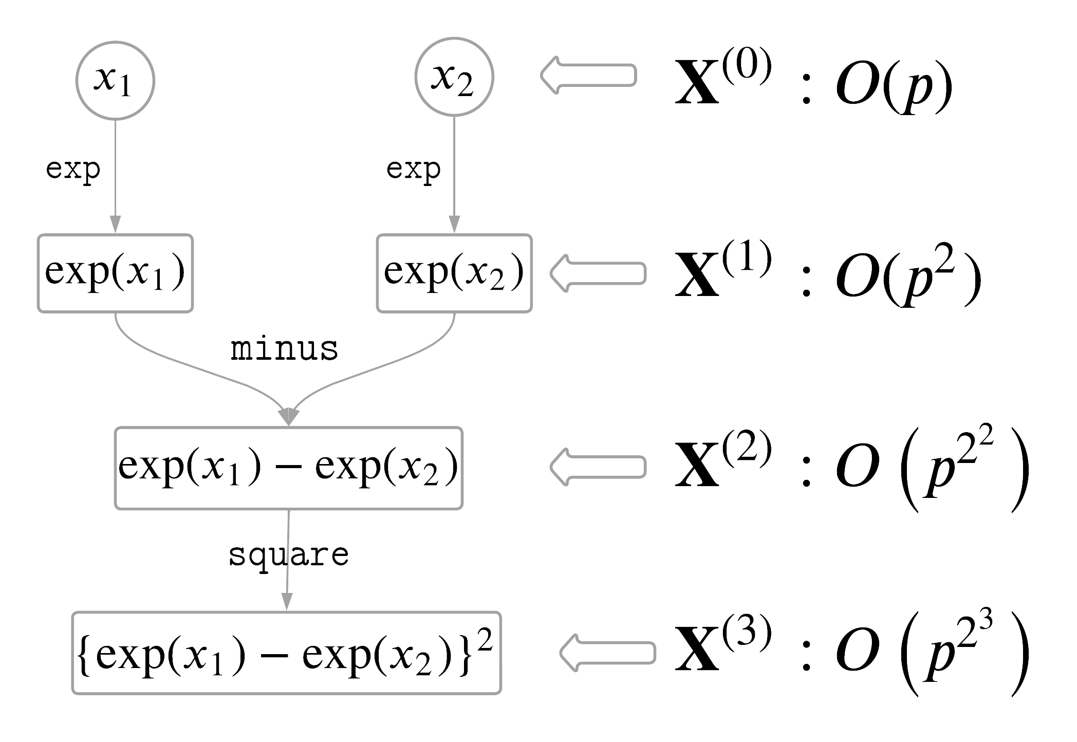
Figure 1: A tree diagram for generating $\{\exp(\bm{x}_{1})-\exp(\bm{x}_{2})\}^{2}$. The dimension of descriptor space increases double exponentially with the composition complexity.

To see how the descriptor space dimension increases with the number of iterations, let $c_{u}$ and $c_{b}$ denote the number of unary and binary operators, respectively, and let $p_{j}$ denote the dimension of the $j$-th descriptor space $\bm{X}^{(j)}$. Note that the dimension of $\bm{X}^{(1)}$ is $p_{1}=c_{u}p+c_{b}p(p-1)/2$, which is on the order of $O(p^{2})$; the dimension of $\bm{X}^{(2)}$ is $p_{2}=c_{u}p_{1}+c_{b}p_{1}(p_{1}-1)/2\approx O(p^{2\cdot 2})=O(p^{2^{2}})$; the dimension of $\bm{X}^{(3)}$ is $p_{3}=c_{u}p_{2}+c_{b}p_{2}(p_{2}-1)/2\approx O(p^{2\cdot 2\cdot 2})=O(p^{2^{3}})$. The dimension of descriptor space will increase double exponentially with the number of binary operator compositions, e.g., with $M$ compositions of binary operators on $\bm{X}$ the resulting descriptor space has a dimension of order $O(p^{2^{M}})$. Similarly, the double exponential expansion applies to the number of binary operators $c_{b}$. Excluding redundant descriptors does not prevent this double exponential expansion. As shown in Section 3.4, building $\bm{X}^{(2)}$ from $p=59$ primary features results in an astronomical descriptor space containing over $5.5\times 10^{7}=O(59^{2^{2}})$ descriptors even after removing redundant and non-physical descriptors. In addition, the number of active (intermediate) descriptors will be non-increasing with $M$ as shown in Figure 1: there are four active descriptors $\exp(\bm{x}_{1}),\exp(\bm{x}_{2}),\bm{x}_{3},\bm{x}_{4}$ in $\bm{X}^{(1)}$, but only two active descriptors $\exp(\bm{x}_{1})-\exp(\bm{x}_{2})$ and $\bm{x}_{3}\bm{x}_{4}$ in $\bm{X}^{(2)}$, and two active descriptors $\{\exp(\bm{x}_{1})-\exp(\bm{x}_{2})\}^{2}$ and $\sin(\pi\bm{x}_{3}\bm{x}_{4})$ in $\bm{X}^{(3)}$.

2.2 PAN descriptor selection for OIS model

We propose an iterative descriptor construction and selection procedure PAN for the OIS model, which generates descriptors by iteratively applying operators and selecting the potentially useful intermediate descriptors between each iteration of descriptors synthesis. The iterative descriptor selection procedure excludes irrelevant intermediate descriptors from the descriptor generating step, achieving a progressive variable selection and enabling variable selection based on ab initio primary features. This reduces the dimension of the subsequent descriptor space $\bm{X}^{(m)}$ and mitigates collinearity among the descriptors in comparison to the one-shot descriptor construction approaches.

To describe the method in its most general form, we allow different sets of operators $\mathcal{O}_{m}\subseteq\mathcal{O}$ for each iteration $m=1,\ldots,M$, leading to the descriptor space

$$\mathcal{O}_{M}\circ\mathcal{O}_{M-1}\circ\cdots\circ\mathcal{O}_{2}\circ\mathcal{O}_{1}(\bm{X}).$$ (7)

The framework of our iterative descriptor selection procedure is as follows.

PAN descriptor selection procedure:

1. Repeat the following until at least one descriptor exhibits a strong linear association with the response variable $\bm{y}$ ($i=0$):

   1. Use a nonparametric variable selection procedure to perform descriptor selection on $\bm{X}^{(i)}$ and obtain the selected descriptors ${\bm{X}^{(i)}}^{\prime}$;

   2. Apply the $i$-th operator set $\mathcal{O}_{i}$ on all of the previously selected descriptors, $\bigcup_{m}{\bm{X}^{(m)}}^{\prime}$, yielding a new descriptor space, $\bm{X}^{(i+1)}=\mathcal{O}_{i}(\bigcup_{m}{\bm{X}^{(m)}}^{\prime})$, where $\mathcal{O}_{i}$ can be different for each iteration $i$;

2. Once there exist descriptor(s) that exhibit a strong linear association with response variable $\bm{y}$, use a linear parametric variable selection procedure to perform descriptor selection on $\bm{X}^{(i)}$, and obtain the selected descriptors, $\bm{X}^{\star}\subseteq\bm{X}^{(i)}$.

We keep all the selected descriptors in the main loop to facilitate the creation of high-order complexity descriptors with the help of low-order complexity descriptors. For instance, constructing $\bm{x}_{1}^{3}$ using $\mathcal{O}$ defined in (2) requires us to keep $\bm{x}_{1}\in{\bm{X}^{(0)}}^{\prime}$ selected at the base iteration and $\bm{x}_{1}^{2}\in{\bm{X}^{(1)}}^{\prime}$ selected at the first iteration.

To see how this iterative procedure helps reduce the dimension of descriptor space significantly, let $s_{i}=|{\bm{X}^{(i)}}^{\prime}|$ be the number of descriptors selected in the $i$-th iteration and $p_{i}=|\bm{X}^{(i)}|$ be the dimension of the $i$-th descriptor space. Suppose that the number of selected descriptors is sparse in each iteration, i.e., $s_{i}\ll p_{i}$. Assuming binary operators were used, the dimension of the $(i+1)$-th descriptor space in PAN is on the order of $O(s_{i}^{2})\ll O(p_{i}^{2})$, and this holds for all iteration $i\geq 0$. If we further assume $s_{i}\approx O(p)$ for all $i\geq 0$, where $p=|\bm{X}|$ is the number of primary features, then the dimension of the $(i+1)$-th descriptor space for PAN is on the order of $O(p^{2})$, compared to $O(p^{2^{i+1}})$ for the one-shot methods. Note these assumptions are reasonable according to the discussion in Section 2.1. In the simulation study in Section 3.4 with $p=10$ primary features, we observed that $s_{i}\approx O(10^{1})$ and $p_{i}\approx O(10^{2})$ for all iterations of the PAN procedure. On the contrary, a one-shot method, such as SISSO, generates a descriptor space containing $9.26\times 10^{9}$ descriptors in the same setting.

The use of a nonparametric variable selection procedure in Step 1(a) is necessary because the intermediate descriptors may not have a strong linear association with the response variable. Thus, a method that accounts for model misspecification, such as a nonparametric method, is more suitable for preliminary screening of the intermediate descriptors. In addition, a suitable nonparametric module for PAN needs to account for the geometry embedded in OIS and the unconventional goal of selecting operators along with variables; the next section discusses performance requirements for this step and introduces an implementation of PAN, iBART, that is particularly suitable for OIS. In Step 2, the oracle descriptors are linearly associated with the response. Hence, we employ linear parametric variable selection methods, such as LASSO (Tibshirani, 1996), to reduce false positives and select the final descriptors.

2.3 Choosing nonparametric module in PAN and iBART

In OIS, the ultimate goal is to recover or approximate the true functional relationship between the response and the primary features. This goal together with PAN entails new performance requirements for the nonparametric module in PAN. To illustrate such a need, let us consider a simple OIS model

$$\bm{y}=f^{(M)}(\bm{X})+\bm{\varepsilon}=\sqrt{\bm{x}_{1}+\bm{x}_{2}}+\bm{\varepsilon}.$$ (8)

In traditional nonparametric variable selection problems, the regression model only sees the primary features, $\bm{X}$, and the desired performance is successful identification of the active index set, $\mathcal{S}_{0}=\{1,2\}$. The base iteration of PAN has a similar goal as we would want the selected index set $\hat{\mathcal{S}}$ to be a superset of $\mathcal{S}_{0}$. However, the intermediate descriptor space $\bm{X}^{(m)}$ in the $m$-th iteration consists of nonlinear transformations of the selected primary features $\bm{X}_{\hat{\mathcal{S}}}$, and the active index set is no longer well-defined.

Due to the iterative structure of PAN, a good nonparametric selection method for PAN must be able to generate and identify the $m$-composition descriptors $f_{k}^{(m)}(\bm{X})$ at the $m$-th iteration (i.e., all active intermediate descriptors). To this end, a suitable nonparametric module should satisfy the following PAN criterion:

It selects all of the $m$-composition descriptors that are necessary for constructing the true $M$-composition descriptor, for all $0\leq m\leq M$ iterations.

Taking model (8) as an example, failing to select either $f_{1}^{(0)}=\bm{x}_{1}$ or $f_{2}^{(0)}=\bm{x}_{2}$ in the base iteration will preclude the generation of $f^{(1)}=(\bm{x}_{1}+\bm{x}_{2})$ and $f^{(2)}=\sqrt{\bm{x}_{1}+\bm{x}_{2}}$ in subsequent iterations. The PAN criterion thus favors a “conservative” nonparametric method, in which false positives during selection are allowed but false negatives must not occur in any iteration. Here false positives are defined within each intermediate descriptor space $\bm{X}^{(m)}$.

The literature has provided a rich menu of nonparametric selection methods; however, the asymmetric effect of false positives and false negatives on descriptor selection illustrated by the PAN criterion motivates our choice of tree-based nonparametric approaches. To see this, suppose the true descriptor is $f(\bm{x}_{1})=\log(\bm{x}_{1})$ and the design matrix $\mathcal{O}(\bm{X})$ consists of 1-composition transformations of the primary features $\bm{X}=(\bm{x}_{1},\ldots,\bm{x}_{p})$. A typical nonparametric method aims to identify the oracle primary predictors ($\bm{x}_{1}$ in this case) that associate with $\bm{y}$ through an unknown function $f(\cdot)$, without considering transformations of $\bm{x}_{1}$ as possible candidate predictors. However, the goal in the presence of OIS is to identify the true primary predictors ($\bm{x}_{1}$) and the correct operator composition ($\log(\cdot)$). This goal, in the presence of many non-signal but highly correlated unary transformations of $\bm{x}_{1}$, namely $\sqrt{\bm{x}_{1}},|\bm{x}_{1}|$, etc., is shown to be difficult for many nonparametric methods; see Supplementary Material Section A.2.1 for detailed analyses. Tree-based methods are invariant to monotonic transformations and thus tend to be robust to related transformations that are often piecewise monotonic. Consequently, they may select unary transformations of $\bm{x}_{1}$ in addition to $f(\bm{x}_{1})=\log(\bm{x}_{1})$—such false positives, although increasing the candidate search space, are favorably compatible with the PAN criterion. We next provide a review of BART (Chipman et al., 2010) and describe BART-G.SE (Bleich et al., 2014)—the default nonparametric module in the PAN framework.

BART is a Bayesian nonparametric ensemble tree method for modeling $\bm{y}=f(\bm{X})+\bm{\varepsilon}$, the unknown relationship between a response vector $\bm{y}$ and a set of predictors $\bm{x}_{1},\ldots,\bm{x}_{p}$. More specifically, BART models the regression function $f$ by a sum of regression trees

$$\bm{y}=\sum_{i=1}^{m}g_{i}(\bm{x}_{1},\ldots,\bm{x}_{p};\mathcal{T}_{i},\bm{\mu}_{i})+\bm{\varepsilon},\qquad\bm{\varepsilon}\sim\mathcal{N}_{n}(\bm{0},\sigma^{2}\bm{I}_{n}).$$ (9)

Each binary regression tree $g_{i}$ consists of a tree structure $\mathcal{T}_{i}$ partitioning observations into $B_{i}$ terminal nodes, and a set of terminal parameters $\bm{\mu}_{i}=\{\mu_{i1},\ldots,\mu_{iB_{i}}\}$ attached to these nodes. Observations within a given terminal node $b$ are constrained to have the same terminal parameter $\mu_{ib}$. The prior distributions for $(\mathcal{T}_{i},\bm{\mu}_{i})$ constrain each tree to be small so that each tree contributes to approximate $f$ in a small and distinct fashion. Readers are referred to Chipman et al. (2010) for the full details of BART and posterior sampling.

The primary usage of BART is prediction, and the predicted values $\hat{\bm{y}}$ for $\bm{y}$ serve no purpose in variable selection. However, a variable inclusion rule can be defined based on the variable inclusion proportion $q_{i}$ of $\bm{x}_{i}$, which can be easily estimated from the posterior samples. To this end, we adopt the permutation-based selection threshold based on the permutation null distribution of $\bm{q}=(q_{1},\ldots,q_{p})$ proposed by Bleich et al. (2014).

Specifically, $B$ permutations of the response vector $\bm{y}_{1}^{*},\ldots,\bm{y}_{B}^{*}$ are generated, and a BART model is fitted for each of the permuted response vectors with the same predictors $\bm{x}_{1},\ldots,\bm{x}_{p}$. The variable inclusion proportions from the permuted BART models $\bm{q}_{1}^{*},\ldots,\bm{q}_{B}^{*}$ are then used to create a permutation null distribution for the non-permuted variable inclusion proportion $\bm{q}$. The predictor $\bm{x}_{i}$ is selected if $q_{i}>m_{i}+C^{*}\cdot s_{i}$, where $m_{i}$ and $s_{i}$ are the mean and standard deviation of the permuted variable inclusion proportion $q_{i}^{*}=(q_{i,1}^{*},\ldots,q_{i,B}^{*})$, and $C^{*}=\inf_{C\in\mathbb{R}^{+}}\left\{\forall i,\frac{1}{B}\sum_{b=1}^{B}\mathbb{I}(q_{i,b}^{*}\leq m_{i}+C\cdot s_{i})>1-\alpha\right\}$ is the smallest global standard error multiplier (G.SE) that gives a simultaneous $1-\alpha$ coverage across the permutation null distributions of $q_{i}$ for all predictors. We refer to BART with the permutation-based selection procedure described above as BART-G.SE.

Various BART-related methods have been recently developed (Linero, 2018; Horiguchi et al., 2021; Liu et al., 2021b). They often incorporate sparsity-inducing priors into BART and prove to be highly effective in various tasks. However, it is unclear whether the excellent performance of them developed in traditional settings carries over to being compatible with the PAN criterion. Indeed, we have found that methods aiming at optimally choosing nonparametric variables in traditional settings may incur fewer false positives but have a higher chance to miss the true descriptors in intermediate iterations—such false negatives are devastating in the context of PAN and OIS variable selection. The PAN criterion provides a useful guide in choosing not only the regression method but also the selection rule, for which we recommend BART-G.SE. In our numerical experiments, we vary the nonparametric module in PAN by comparing several recent BART-related methods and other nonparametric selection methods, and find that the proposed iBART, PAN with BART-G.SE as the nonparametric module, is particularly well suited for OIS variable selection and tends to give the best overall performance; see the Supplementary Material for numerical results and a comprehensive discussion.

2.4 Practical consideration and the algorithm

The operators in $\mathcal{O}$ in (2) can be classified into the unary operators $\mathcal{O}_{u}=\{I,\exp,\log,|\cdot|,\sqrt{},^{-1},^{2},\sin(\pi\cdot),\cos(\pi\cdot)\}$ and the binary operators $\mathcal{O}_{b}=\{+,-,\times,/,|-|\}$, each posing different challenges to descriptor selection. The unary operators $\mathcal{O}_{u}$ induce strong collinearity among the engineered descriptors; for instance, $\text{Cor}(\bm{x}_{1}^{2},|\bm{x}_{1}|)>0.9$ when $\bm{x}_{1}\sim\mathcal{N}_{n}(\bm{0},\bm{I})$ with $n=200$. The binary operators $\mathcal{O}_{b}$ increase the descriptor space dimension double exponentially and generate complex nonlinear descriptors. These two issues are compounded when the two operator sets are used together. Therefore, we propose to decouple the two operator sets and alternate them, leading to two special cases of (7):

$$\mathcal{O}_{A_{u}}^{(M)}(\bm{X}) =\underbrace{\cdots\mathcal{O}_{b}\circ\mathcal{O}_{u}\circ\mathcal{O}_{b}\circ\mathcal{O}_{u}}_{M\text{ times}}(\bm{X}),$$ (10)

$$\mathcal{O}_{A_{b}}^{(M)}(\bm{X}) =\underbrace{\cdots\mathcal{O}_{u}\circ\mathcal{O}_{b}\circ\mathcal{O}_{u}\circ\mathcal{O}_{b}}_{M\text{ times}}(\bm{X})=\mathcal{O}_{A_{u}}^{(M-1)}\circ\mathcal{O}_{b}(\bm{X}).$$ (11)

In addition to the binary operators identified earlier, we include an additional binary operator, $\pi_{1}:\mathbb{R}^{2}\to\mathbb{R}$, defined by $\pi_{1}(a,b)=a$, which allows intermediate descriptors to be passed down unchanged. Note the two alternating descriptor spaces $\mathcal{O}_{A_{u}}^{(M)}(\bm{X})$ and $\mathcal{O}_{A_{b}}^{(M)}(\bm{X})$ are not equivalent to the full descriptor space $\mathcal{O}^{(M)}(\bm{X})$ with the same composition complexity $M$. However, one can show that $\mathcal{O}_{A_{u}}^{(M_{u})}(\bm{X})$ and $\mathcal{O}_{A_{b}}^{(M_{b})}(\bm{X})$ can recover $\mathcal{O}^{(M)}(\bm{X})$ with some $M_{u}>M$ and $M_{b}>M$, respectively. This is formally described in the theorem below and its proof is available in Supplementary Material Section D.

Theorem 2.1.

Let $\bm{X}=(\bm{x}_{1},\ldots,\bm{x}_{p})\in\mathbb{R}^{n\times p}$ be a primary feature space and $\mathcal{O}$ be a set of operators such that it can be partitioned into a unary operator set $\mathcal{O}_{u}$ and a binary operator set $\mathcal{O}_{b}$. Suppose that $I\in\mathcal{O}_{u}$ and $\pi_{1}\in\mathcal{O}_{b}$. Then for any $M\in\mathbb{N}$, there exists $M_{u}\geq M$ and $M_{b}\geq M$ such that $\mathcal{O}_{A_{u}}^{(M_{u})}(\bm{X})\supseteq\mathcal{O}^{(M)}(\bm{X})$ and $\mathcal{O}_{A_{b}}^{(M_{b})}(\bm{X})\supseteq\mathcal{O}^{(M)}(\bm{X})$, respectively.

For instance, the 2-composition descriptor space $\mathcal{O}^{(2)}(\bm{X})$ generated using (4) contains descriptors such as $f_{1}=(x_{i}^{2}+x_{j}^{2})$ and $f_{2}=(x_{i}+x_{j})^{2}$. These two descriptors can be generated using $\mathcal{O}_{A_{b}}^{(M)}(\bm{X})$ in (11): $f_{1}=\texttt{add}(\texttt{square}\circ\pi_{1}(x_{i},x_{j}),\texttt{square}\circ\pi_{1}(x_{j},x_{i}))\in\mathcal{O}_{A_{b}}^{(3)}(\bm{X})$ and $f_{2}=\texttt{square}\circ\texttt{add}(x_{i},x_{j})\in\mathcal{O}_{A_{b}}^{(2)}(\bm{X})$. Using (10), $f_{1}$ and $f_{2}$ can also be generated as $f_{1}=\texttt{add}(\texttt{square}(x_{i}),\texttt{square}(x_{j}))\in\mathcal{O}_{A_{u}}^{(2)}(\bm{X})$ and $f_{2}=\texttt{square}\circ\texttt{add}(I(x_{i}),I(x_{j}))\in\mathcal{O}_{A_{u}}^{(3)}(\bm{X})$. As such, under the $M$-composition OIS model in (5), one may consider using $\mathcal{O}^{(M)}$, $\mathcal{O}_{A_{u}}^{(M_{u})}(\bm{X})$, or $\mathcal{O}_{A_{b}}^{(M_{b})}(\bm{X})$ as long as they contain the true descriptors. In what follows we will focus on $\mathcal{O}_{A_{u}}^{(M)}(\bm{X})$ and $\mathcal{O}_{A_{b}}^{(M)}(\bm{X})$ instead of $\mathcal{O}^{(M)}$ for their aforementioned advantages.

We adopt the descriptor generating strategies in (10) and (11) for different scenarios. In particular, if the primary features $\bm{X}$ are believed to generate the model through their intricate interactions that will be captured by binary operators and compositions of such binary operators, we recommend (11). This is often the case in real-world applications, such as in Section 4, where the domain scientists have chosen a large set of potentially useful primary features, and unary transformations of these primary features are less interpretable and thus less desired. If such prior knowledge is not available and the relevant functional form of primary features is unknown, as in Section 3, we would recommend (10) to first identify such functional forms by selecting between unary descriptors.

The stopping criterion in Step 1 can be easily modified depending on practical needs. For example, we can specify the maximum composition complexity $M_{\max}$, like SISSO, or implement a data-driven criterion that terminates Step 1 when there exists a descriptor such that its absolute correlation with response variable $\bm{y}$ exceeds a pre-specified threshold $\rho_{\max}$ that is close to 1. We note that iBART allows larger $M_{\max}$ than SISSO as iBART does not rely on one-short feature engineering, and the use of $\rho_{\max}$ allows early termination.

It is also common in practice that one may only want to select $k$ descriptors for easy interpretation, such as $k\leq 5$. If the cardinality of the selected descriptors $\bm{X}^{\star}$ is greater than $k$, then an $\ell_{0}$-penalized regression may be used to choose the best $k$ descriptors.

We allow user-specified options for these considerations when implementing iBART, summarized in Algorithm 1; an R package for iBART is available at https://github.com/mattsheng/iBART. The following default settings will be used in our experiments. We use the BART-G.SE thresholding variable selection procedure implemented in the R package bartMachine to perform nonparametric variable selection for Step 1(a) in PAN and use LASSO implemented in the R package glmnet to perform parametric variable selection for Step 2 in PAN. For BART-G.SE, we set the number of trees to 20 that is recommended by Bleich et al. (2014), the number of burn-in samples to 10,000, the number of posterior samples to 5,000, the number of permutations of the response to 50, and the rest of the parameters to the default values. With these values, our Markov chain Monte Carlo (MCMC) runs appear to have reached a sufficient number of iterations in our experiments. We choose the penalty term $\lambda$ in LASSO by minimizing the mean squared error loss through a 10-fold cross-validation procedure and set the other parameters to the default values. Unreported results using real data indicate that other tuning methods to debias LASSO yield similar performance. The algorithm terminates if the composition complexity $M$ reaches $M_{\max}=4$ or the maximum absolute correlation $|\rho|$ reaches $\rho_{\max}=0.95$, whichever occurs first. Setting $M_{\max}$ to 4 appears sufficient for the considered materials GWAS application as descriptors with more complexity become challenging to interpret.

Input: $\rho_{\max}\in(0,1)=$ maximum absolute correlation with the response variable;

$M_{\max}=$ maximum composition complexity;

Lzero = whether to perform $\ell_{0}$-penalized regression;

$k=$ number of selected descriptors by $\ell_{0}$-penalized regression. Only required when Lzero == TRUE.

Output: $\bm{X}_{k}^{\star}$: selected descriptors

Data: $\bm{X}$: primary features; $\mathcal{O}_{u}$: set of unary operators; $\mathcal{O}_{b}$: set of binary operators; $\bm{y}$: response vector

1 $M=0$

2 $\rho=\max_{\bm{x}\in\bm{X}^{(M)}}\text{cor}(\bm{x},\bm{y})$

3 while $M\leq M_{\max}$ or $|\rho|\leq\rho_{\max}$ do

4       ${\bm{X}^{(M)}}^{\prime}\leftarrow$ BART-G.SE selected descriptors on $\bm{X}^{(M)}$

5       $\bm{X}^{(M+1)}\leftarrow\mathcal{O}_{M+1}\left(\cup_{i}{\bm{X}^{(i)}}^{\prime}\right)$

6       $M\leftarrow M+1$

7       $\rho\leftarrow\max_{\bm{x}\in\bm{X}^{(M)}}\text{cor}(\bm{x},\bm{y})$

8 end while

9$\bm{X}^{\star}\leftarrow$ LASSO selected descriptors on $\bm{X}^{(M)}$

10 if Lzero == TRUE and $|\bm{X}^{\star}|>k$ then

11       $\bm{X}_{k}^{\star}\leftarrow$ best $k$ descriptors from $\ell_{0}$-penalized regression

12 end if

13else

14       $\bm{X}_{k}^{\star}\leftarrow\bm{X}^{\star}$

15 end if

Algorithm 1 iBART

3 Simulation

3.1 Outline

In Sections 3.2 and 3.3 we demonstrate that the employed BART-G.SE tends to satisfy the PAN criterion when selecting unary and binary operators, respectively, and evaluate its false positives. Section 3.4 assesses iBART relative to several existing descriptor selection methods in view of the PAN criterion and OIS variable selection accuracy using a complex simulation setting. Section 3.5 showcases the robustness of iBART in the initial input dimension $p$. Section 3.6 examines the performance of iBART when the operator set $\mathcal{O}$ can not generate the ground truth model. We use Algorithm 1 and the default settings described in Section 2.4 when implementing iBART, unless stated otherwise. Each simulation is replicated 100 times. We also compare variants of iBART by varying the nonparametric module; see the Supplementary Material for details.

3.2 Unary operators

We consider all unary transformations of five primary features $\bm{X}=(\bm{x}_{1},\ldots,\bm{x}_{5})$, i.e., the descriptor space is $\mathcal{O}_{u}(\bm{X})=\bigcup_{i=1}^{5}\left\{\bm{x}_{i},\bm{x}_{i}^{-1},\bm{x}_{i}^{2},\sqrt{\bm{x}_{i}},\log(\bm{x}_{i}),\exp(\bm{x}_{i}),|\bm{x}_{i}|,\sin(\pi\bm{x}_{i}),\cos(\pi\bm{x}_{i})\right\}$. For each unary operator $u_{j}\in\mathcal{O}_{u}$, we generate the response vector by

$$\bm{y}=10u_{j}(\bm{x}_{1})+\bm{\varepsilon},\qquad\bm{\varepsilon}\sim\mathcal{N}_{n}(\bm{0},\bm{I}),$$ (12)

with sample size $n=200$, yielding nine independent models in total. We draw the primary features $\bm{X}$ independently from the standard normal distribution if the domain of $u_{j}$ is $\mathbb{R}$, and the Lognormal(2, 0.5) distribution if the domain is $\mathbb{R}_{\geq 0}$.

The left plot in Figure 2(a) shows the number of true positives (TP) of BART-G.SE. For each of the nine models in (12), the true descriptor is selected 100/100 times. This suggests that BART-G.SE is capable of identifying the true descriptor with high probability when the descriptor space is populated with unary operators $\mathcal{O}_{u}$. Other nonparametric methods did not select all TP 100/100 times for all nine scenarios, failing the PAN criterion; see the Supplementary Material for further results and discussion.

The left plot in Figure 2(b) shows the number of FP of BART-G.SE for each simulation setting. Although BART-G.SE is capable of capturing the true descriptor with high probability, it also selects some non-signal descriptors in some cases. The number of FP is especially high when the true descriptor is $\bm{x}_{1}$, $|\bm{x}_{1}|,\exp(\bm{x}_{1}),\log(\bm{x}_{1}),\bm{x}_{1}^{2}$, or $\sqrt{\bm{x}_{1}}$. This is due to high collinearity among these six descriptors. In particular, the empirical Pearson correlation between $\log(\bm{x}_{1})$ and $\sqrt{\bm{x}_{1}}$ is over 0.99 under simulation setting (12) and thus some false positives are expected. Selecting inactive descriptors in one iteration is less of a concern in variable selection with OIS as they do not constitute misspecified models, and can be further screened out during Step 2 of PAN.

3.3 Binary operators

In this simulation study, we apply binary operators $\mathcal{O}_{b}=\{+,-,\times,/,|-|,\pi_{1}\}$ on the five primary features $\bm{X}=(\bm{x}_{1},\ldots,\bm{x}_{5})$. The descriptor space $\mathcal{O}_{b}(\bm{X})\in\mathbb{R}^{200\times 55}$ contains all binary transformations of all possible pairs of the five primary features. For each binary operator $b_{j}\in\mathcal{O}_{b},$ we generate the response vector by

$$\bm{y}=10b_{j}(\bm{x}_{1},\bm{x}_{2})+\bm{\varepsilon},\qquad\bm{\varepsilon}\sim\mathcal{N}_{n}(\bm{0},\bm{I}),$$ (13)

with sample size $n=200$, yielding a total of six independent models. We generate the primary features $\bm{X}$ following $\bm{x}_{1},\ldots,\bm{x}_{5}\overset{\text{i.i.d.}}{\sim}\mathcal{N}_{n}(\bm{0},\bm{I}).$

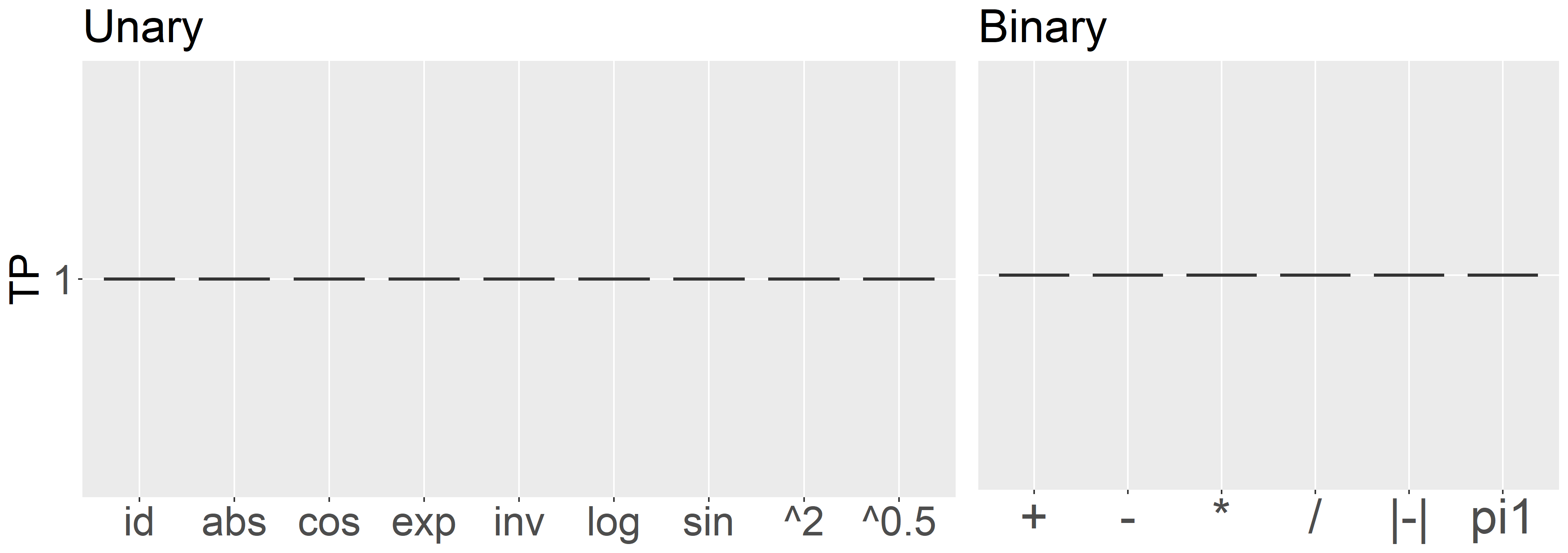
(a) TP

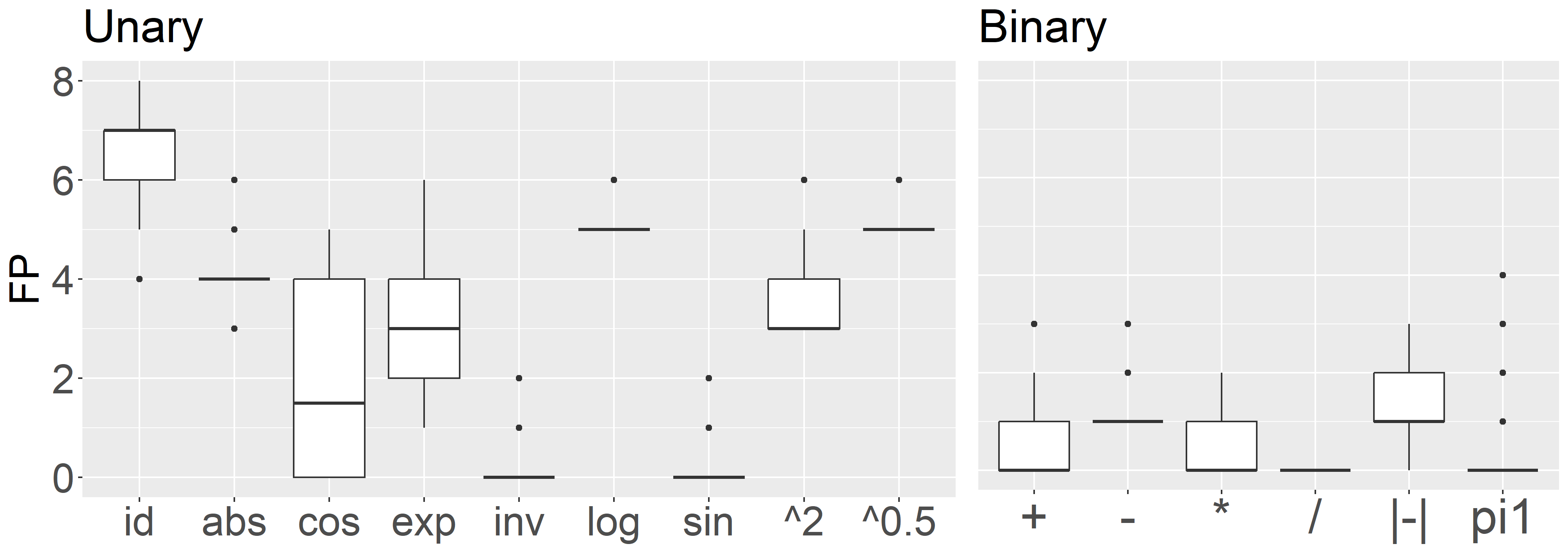
(b) FP

Figure 2: Boxplots of TP and FP over 100 simulation replicates under (12) and (13).

The right plot in Figure 2(a) shows the number of TP for each of the six models in (13). BART-G.SE is able to identify the true binary descriptor 100/100 times in all six settings, similar to earlier observations in Section 3.2. The right plot in Figure 2(b) shows that BART-G.SE may also select some irrelevant descriptors but considerably fewer than in Section 3.2. In particular, when the true descriptor is $(\bm{x}_{1}-\bm{x}_{2})$, BART-G.SE correctly selects $(\bm{x}_{1}-\bm{x}_{2})$ but also selects $|\bm{x}_{1}-\bm{x}_{2}|$ 100/100 times. Unlike in Section 3.2, the inclusion of $|\bm{x}_{1}-\bm{x}_{2}|$ is not due to high correlation between $|\bm{x}_{1}-\bm{x}_{2}|$ and $(\bm{x}_{1}-\bm{x}_{2})$. In fact, their empirical Pearson correlation is merely 0.07. We suspect that $|\bm{x}_{1}-\bm{x}_{2}|$ was selected due to its piecewise monotonicity in $(\bm{x}_{1}-\bm{x}_{2})$ that tends to be invariant to tree-based methods. Similarly, BART-G.SE selects both $(\bm{x}_{1}-\bm{x}_{2})$ and $|\bm{x}_{1}-\bm{x}_{2}|$ with high probability when the true descriptor is $|\bm{x}_{1}-\bm{x}_{2}|$. When the true descriptor is $(\bm{x}_{1}+\bm{x}_{2})$, $\bm{x}_{1}\times\bm{x}_{2}$, $\bm{x}_{1}/\bm{x}_{2}$, or $\pi_{1}(\bm{x}_{1},\bm{x}_{2})$, the FP of BART-G.SE is nearly zero. This shows that BART-G.SE is not too conservative when high collinearity does not exist.

Our investigation using unary and binary descriptors suggests that the permutation threshold of BART-G.SE tends to satisfy the PAN criterion without being too conservative, making it a good candidate for PAN and OIS variable selection. We next use a more complex simulation to assess iBART in view of the PAN criterion and OIS selection accuracy.

3.4 Complex descriptors with high-order compositions

In this section, we compare iBART with existing approaches under a complex model and demonstrate superior performance of iBART. We use the following model

$$\bm{y}=15\{\exp(\bm{x}_{1})-\exp(\bm{x}_{2})\}^{2}+20\sin(\pi\bm{x}_{3}\bm{x}_{4})+\bm{\varepsilon},\qquad\bm{\varepsilon}\sim\mathcal{N}_{n}(\bm{0},\sigma^{2}\bm{I}),$$ (14)

with $n=250$, $p=10$, and $\sigma=0.5$. Here the number of primary features $p$ is set to a relatively small number since competing one-shot methods cannot complete the simulation when $p\geq 20$ due to the ultra-high dimension of their descriptor spaces. In Section 3.5, we demonstrate that iBART scales well in $p$ and gives a robust performance. We use the operator set $\mathcal{O}$ defined in (2) with $\pi_{1}$, and the primary feature vectors $\bm{x}_{i}$ are drawn independently from a uniform distribution, namely, $\bm{x}_{1},\ldots,\bm{x}_{p}\overset{\text{i.i.d.}}{\sim}\text{U}_{n}(-1,1).$ Section B of Supplementary Material demonstrates the effect of dependent primary features on iBART and other methods using the same functional relationship in (14).

iBART is implemented in R based on Algorithm 1 in Section 2.4 using the default settings. We chose the descriptor generating process (10) in Section 3 since the i.i.d. primary features do not show strong collinearity. Two versions of iBART are considered: iBART without and with $\ell_{0}$-penalized regression, labeled as “iBART” and “iBART$+\ell_{0}$”, respectively. The $\ell_{0}$-penalization finds the best subset of $k$ variables from the set of selected variables using the Akaike information criterion (AIC) with $k\in\{1,2,3,4\}$. We compare the performance of iBART and iBART$+\ell_{0}$ with SISSO and LASSO. SISSO is implemented using the Fortran 90 program published by Ouyang et al. (2018) on GitHub with the following settings: the descriptor magnitude allowed in the descriptor space is set to $[1\times 10^{-6},1\times 10^{5}]$; the size of the SIS-selected subspace is set to 20; the operator composition complexity $M$ is set to 3; the maximum number of operators in a descriptor is set to 6; and the number of selected descriptors $k\in\{1,2,3,4\}$ is tuned by AIC. The R package glmnet is used to implement LASSO and the penalty parameter $\lambda$ is tuned via 10-fold cross-validation to minimize the mean squared error loss. Since the size of $\mathcal{O}^{(3)}(\bm{X})$ exceeds the limit of an R matrix, we give LASSO an advantage by reducing the descriptor space to $\mathcal{O}_{u}\circ\mathcal{O}\circ\mathcal{O}(\bm{X})$ that aligns with the true data-generating process. We also utilize the $\ell_{0}$-penalized regression step as in SISSO and iBART+$\ell_{0}$ for LASSO, leading to LASSO$+\ell_{0}$.

For each method, we calculate the number of TP selections, FP selections, and false negative (FN) selections. We use the $F_{1}$ score as an overall metric to quantify the performance of each method: $F_{1}=2\cdot\frac{\text{Precision}\cdot\text{Recall}}{\text{Precision}+\text{Recall}},$ where $\text{Precision}=\frac{\text{TP}}{\text{TP}+\text{FP}}$ and $\text{Recall}=\frac{\text{TP}}{\text{TP}+\text{FN}}$. The value $F_{1}=1$ means correct identification of the true model without having any FP and FN. In this simulation, the two TPs are $f_{1}(\bm{X})=\{\exp(\bm{x}_{1})-\exp(\bm{x}_{2})\}^{2}$ and $f_{2}(\bm{X})=\sin(\pi\bm{x}_{3}\bm{x}_{4})$.

As shown in Figure 3A, both iBART-based methods achieve very high $F_{1}$ scores, with a median $F_{1}$ of 0.8 and 1 for iBART and iBART$+\ell_{0}$, respectively. In particular, both iBART and iBART$+\ell_{0}$ have 2 TPs in all simulations while incurring an average FP of 0.93 and 0.3, respectively. This demonstrates that iBART satisfies the PAN criterion in all iterations as it is able to identify the 2 TPs 100/100 times in simulations. Furthermore, iBART$+\ell_{0}$ gives a very low FP, scoring a perfect $F_{1}$ score 75/100 times. LASSO-based methods and SISSO have lower $F_{1}$ scores than iBART and iBART$+\ell_{0}$ but for different reasons. LASSO selects 37.65 descriptors on average, and the 2 TPs are always selected. This means that LASSO also enjoys the PAN criterion but its $F_{1}$ score is hindered by the large number of FP. With the help of the $\ell_{0}$-penalized regression, LASSO$+\ell_{0}$ reduces the average number of FP from 35.65 to 2 while maintaining 2 TPs 100/100 times, substantially increasing the $F_{1}$ score to 0.67, the third-highest score but still considerably lower than iBART and iBART$+\ell_{0}$. SISSO, on the other hand, has only 1 TP but 3 FPs in all simulations, which unfortunately does not satisfy the PAN criterion. In particular, SISSO can identify $\sin(\pi\bm{x}_{3}\bm{x}_{4})$ 100/100 times but always selects a false signal, $|\exp(\bm{x}_{1})-\exp(\bm{x}_{2})|$, a descriptor that has an absolute correlation over 0.9 with the TP, $\{\exp(\bm{x}_{1})-\exp(\bm{x}_{2})\}^{2}$. In summary, both iBART-based and LASSO-based methods satisfy the PAN criterion but LASSO-based methods incur more FPs. SISSO, however, fails to identify one of the two descriptors 100/100 times but selects a highly correlated counterpart, indicating its relatively weakened ability to distinguish the true descriptor when there are descriptors highly correlated with the TP. Results not reported here show that replacing BART-G.SE with LASSO in the PAN framework missed TPs with high probability even at the base iteration, indicating the importance of nonparametric variable selection in PAN.

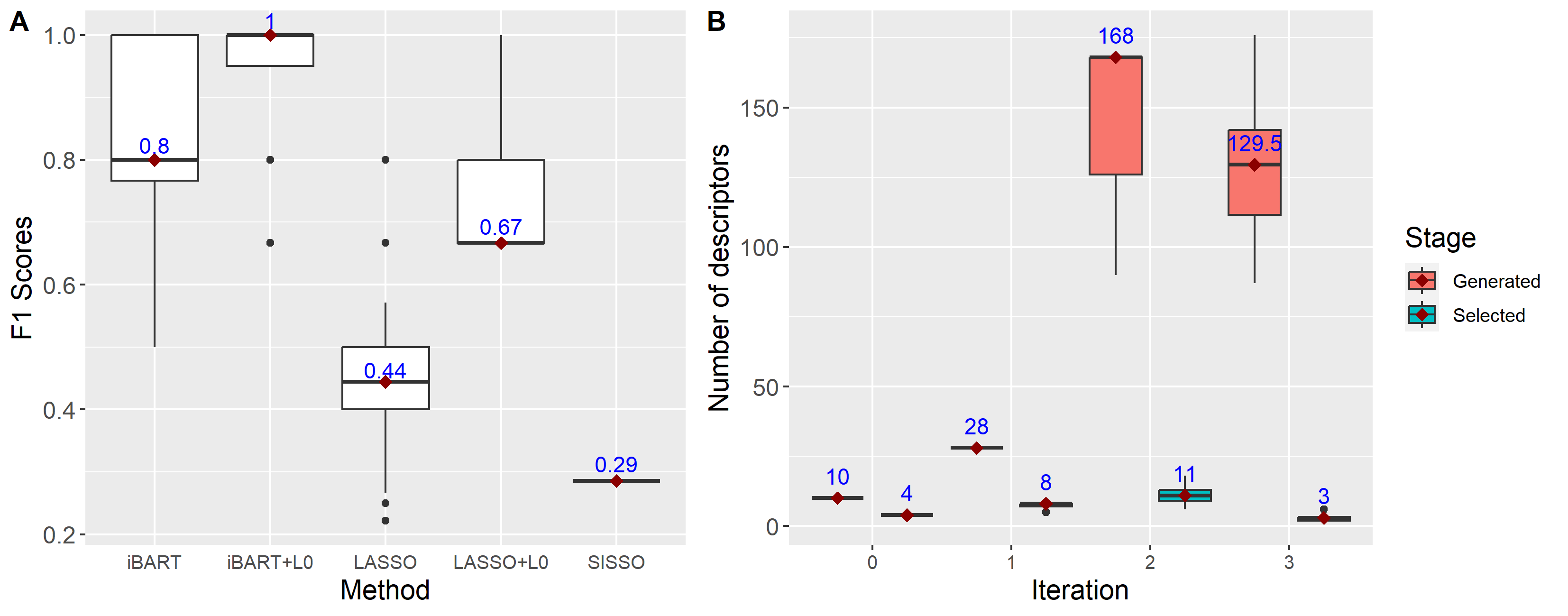
Figure 3: Left: Boxplots of $F_{1}$ scores over 100 simulations for different methods under Model (14). Right: Boxplots of iBART generated and selected descriptors in each iteration.

To gain insight into the scalability of iBART, Figure 3B shows the boxplots of the number of iBART generated and selected descriptors in each iteration. Throughout the 100 simulation replicates, iBART generates no more than $168\leq 2p^{2}$ descriptors, which is significantly less than the number of descriptors generated by SISSO ($9.26\times 10^{9}$) and LASSO ($1.2\times 10^{6}$). Such dimension reduction not only reduces runtime and memory usage but also enables iBART to tackle data with much larger $p$, as we show in Sections 3.5 and 4.

3.5 Large $p$

In this section, we demonstrate that the performance of iBART is robust to increase in input dimension $p$ while one-shot descriptor selection methods are not. Under Model (14) with $p=20$, SISSO with the same parameter settings in the preceding section generates more than $3.8\times 10^{11}$ descriptors and failed to complete one simulation within 24 hours on a server with 1.3TB of memory and 40 CPU cores available to SISSO. LASSO, on the other hand, failed at $p=20$ since the glmnet function in the R package glmnet cannot handle a matrix of size $250\times(1.57\times 10^{7})$. The proposed method iBART instead scales well in the input dimension $p$ partly because of the efficient dimension reduction via the PAN strategy. In particular, when $p=20$, iBART took an average of 497 seconds to finish, and its memory usage peaks out at 10.85 GB in 100 simulation replicates.

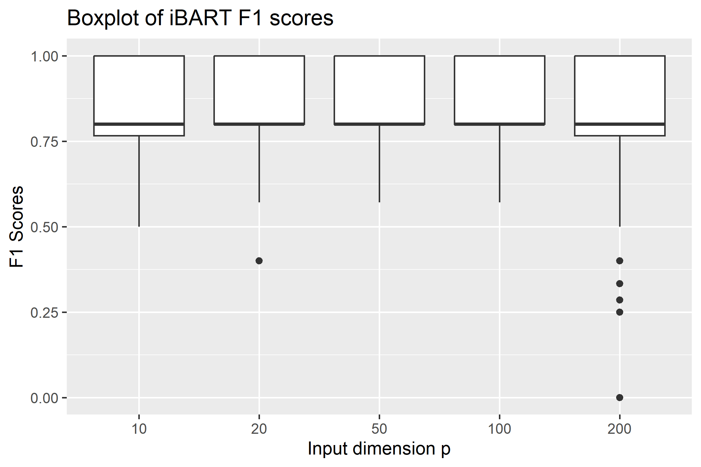
Figure 4: Boxplot of $F_{1}$ scores for iBART under Model (14) with $p\in\{10,20,50,100,200\}$.

We implement iBART for $p\in\{10,20,50,100,200\}$ using the same simulation settings in Section 3.4. Figure 4 shows that iBART’s $F_{1}$ score is robust to the increase in $p$. In fact, benefiting from the ab initio mechanism through the PAN strategy, the performance of iBART would be identical for varying $p$ as long as it selects $\bm{x}_{1},\bm{x}_{2},\bm{x}_{3},\bm{x}_{4}$ in the first iteration, which is often the case based on Figure 4 at least under the current simulation setting. We acknowledge that the stability of the $F_{1}$ scores across different values of $p$ may be attributed, in part, to the relatively small noise standard deviation. In contrast, one-shot descriptor selection methods suffer significantly from just a small increase in the input dimension $p$ since the descriptor space increases double exponentially in $p$. One way for one-shot description selection methods to circumvent the ultra-high dimension issue is to reduce the maximum composition complexity $M_{\text{max}}$. However, this undesirably rules out descriptors with the correct composition complexity. For example, the descriptor in (14) $f_{1}(\bm{x})=\{\exp(\bm{x}_{1})-\exp(\bm{x}_{2})\}^{2}$ requires at least 3 compositions of operators and reducing $M_{\text{max}}$ to 2 means that $f_{1}(\bm{x})$ would never be generated and hence would never be selected. Thus, in a complex scenario, one-shot descriptor selection methods cannot generate and select the complex descriptors unless $p$ is small. We considered a small $p=10$ in the preceding section to accommodate such limitation of one-shot methods.

3.6 Model misspecification

In this section, we examine the behavior of iBART when the operator set $\mathcal{O}$ is not sufficient to generate the data-generating function. We generate data from the model $\bm{y}=\bm{x}_{1}^{1.7}+\bm{\varepsilon}$ with $\bm{\varepsilon}\sim\mathcal{N}_{n}(\bm{0},\bm{I})$, $n=250$, $p=10$, use the same operator set $\mathcal{O}$ as in Section 3.4, and draw the primary features from a uniform distribution, i.e., $\bm{x}_{1},\ldots,\bm{x}_{p}\overset{\text{i.i.d.}}{\sim}\text{U}_{n}(0,3).$ In this simulation, iBART iterates once after screening the primary features. Since iBART only selects $\bm{x}_{1}$ in the first iteration, 100/100 times, it does not apply the binary operators in $\mathcal{O}$.

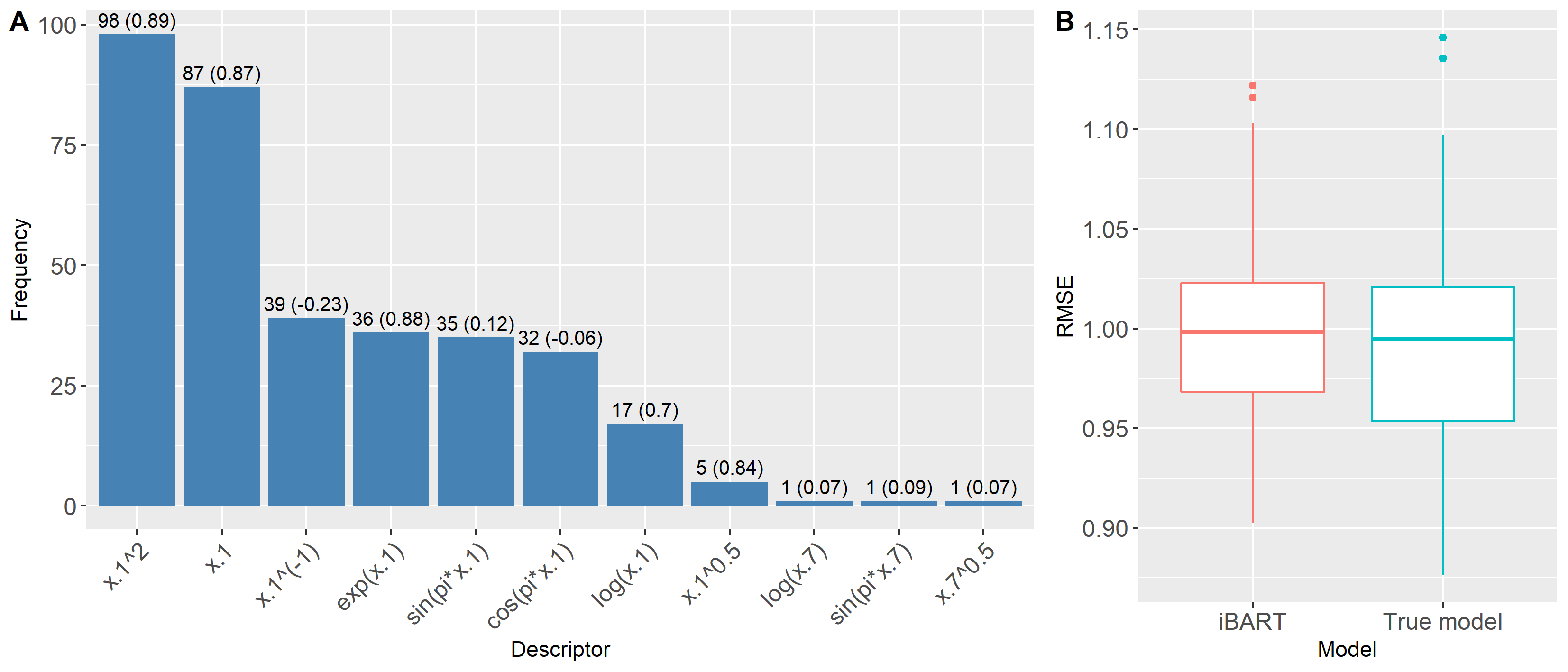
Figure 5: Left: frequency (average Pearson correlation with $\bm{x}_{1}^{1.7}$) of iBART selected descriptors. Right: root mean squares error (RMSE) of iBART models and the true models.

In contrast to the preceding sections, the computation of true and false positives, as well as the $F_{1}$ scores, is not feasible here due to the model specification by design. To evaluate the performance of our method, Figure 5A shows the frequency of unique descriptors selected by iBART and the average Pearson correlation between the selected descriptor and $\bm{x}_{1}^{1.7}$ in parentheses. Note that multiple descriptors might be selected in one replication, and therefore the sum of frequencies exceeds 100. We can see that, although the true descriptor $\bm{x}_{1}^{1.7}$ is not in the candidate descriptor space, iBART selects highly correlated descriptors from the candidate space, including $\bm{x}_{1}^{2}$ for 98% of the time and $\bm{x}_{1}$ for 87% of the time. Figure 5B shows that the RMSE of the iBART selected models does not deviate much from the RMSE of the true model, indicating a similar explanatory power. These observations suggest that when the employed operator space is not sufficient to generate the ground truth, iBART is capable of selecting a model that closely resembles the true model, at least in the considered simulation setting. This is reassuring as in many applications of OIS, such as the one in Section 4, the goal is precisely to find an accurate but interpretable model that well approximates complex real-world physical systems.

4 Application to single-atom catalysis

We apply the proposed method to analyze a single-atom catalysis dataset (O’Connor et al., 2018) in which the goal is to identify physical descriptors that are associated with the binding energy of metal-support pairs calculated by density functional theory (DFT). Single-atom catalysts are popular in modern materials science and chemistry as they offer high reactivity and selectivity while maximizing utilization of the expensive active metal component (Yang et al., 2013; O’Connor et al., 2018; Wang et al., 2018). However, single-atom catalysts suffer from a lack of stability caused by the tendency for single metal atoms to agglomerate in a process called sintering. To prevent sintering in single-atom catalysts, one can tune the binding strength between single metal atoms and oxide supports. While first principle simulations can calculate the binding energy for given metal-support pairs, modeling their association requires explicit statistical modeling and is key to aid the design of single-atom catalysts that are robust against sintering. Feature engineering leads to physical descriptors constructed using mathematical operators and physical properties of the supported metal and the support, and gains popularity in materials informatics as the obtained descriptors are interpretable and provide insights into the underlying physical relationship. The key challenge is to select the most relevant physical properties among large-scale candidate predictors that have explanatory and predictive power to the binding energy; often the sample size is small as first principle simulations are computationally intensive.

The data comprise binding energy of $n=91$ metal-support pairs and $p=59$ physical properties of these metal-support pairs, in which the binding energy serves as the response $\bm{y}$ while the 59 physical properties constitute the primary features $\bm{X}=(\bm{x}_{1},\ldots,\bm{x}_{59})$. We use the operator set given in (2) but exclude $\sin(\pi\cdot)$ and $\cos(\pi\cdot)$ because they are not physically meaningful in this data application.

In this analysis, we compare the best $k$ descriptors ($k=1,\ldots,5)$ of iBART$+\ell_{0}$ (referred to as iBART for brevity), SISSO, and the method proposed in O’Connor et al. (2018). The method proposed in O’Connor et al. (2018) combines LASSO with extensive domain knowledge; in particular, they rule out a substantial proportion of less promising descriptors using expert knowledge of single-atom catalysis. Such expert-guided, tailored dimension reduction is not needed for SISSO or iBART, but is necessary for LASSO-type methods because the astronomical size of $\mathcal{O}^{(2)}(\bm{X})$ in this application far exceeds the maximum matrix size allowed in many modern programming languages. We refer to O’Connor et al. (2018) as LASSO^⋆ to distinguish it from LASSO$+\ell_{0}$ implemented in Section 3.4. To enhance interpretability, we eliminate non-physical descriptors, such as $\textit{volumn}+\textit{speed}$, by automatically comparing the units of the constructed descriptors. Results without this constraint are reported in the Supplementary Material, showing that this constraint does not alter our conclusions when comparing methods but substantially improves the interpretability of the identified model.

For iBART, we follow the settings described in Section 2.4 and use the descriptor generating process (11). The SISSO parameters are set as followed. The maximum number of descriptors allowed in a model is set to 5; the descriptor magnitude allowed in the descriptor space is set to $[1\times 10^{-8},1\times 10^{8}]$; the size of the SIS-selected subspace is set to 40; the composition complexity $M$ is cap at 2 because $\mathcal{O}^{(3)}(\bm{X})$ and higher complexity space exceed the maximum number of elements allowed in a Fortran 90 array. The LASSO^⋆ procedure is implemented using the MATLAB code published by O’Connor et al. (2018) with all parameters left as default.

Each method’s performance is assessed using out-of-sample RMSE, runtime, and the number of generated descriptors. To calculate out-of-sample RMSE, we randomly partition the $n=91$ observations into a 90% training set (82 samples) and a 10% testing set (9 samples) and repeat this process 50 times. For brevity, we herein refer to out-of-sample RMSE as RMSE.

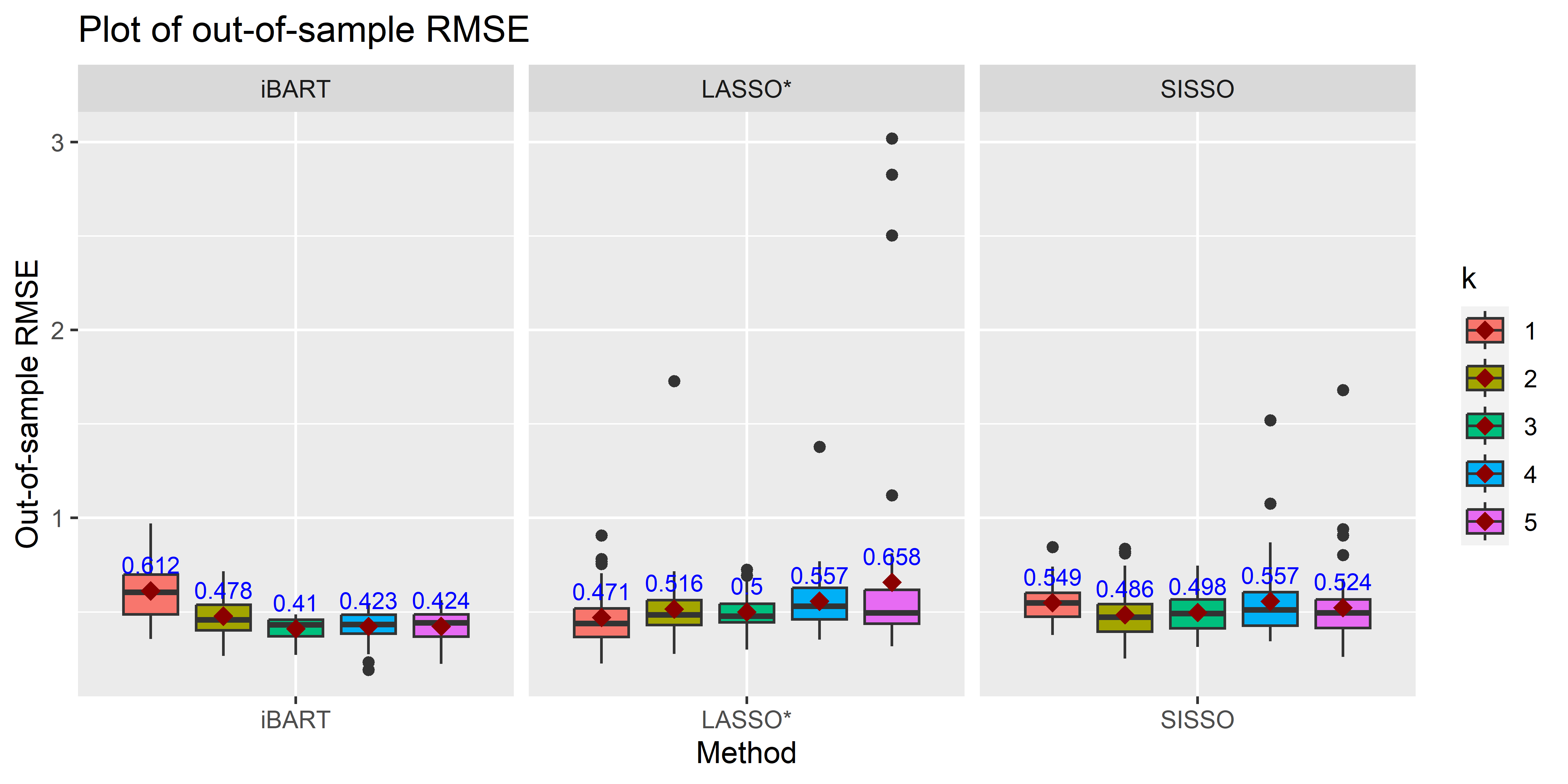
Figure 6: Boxplot of the out-of-sample RMSE for each method across 50 random partitions with $1\leq k\leq 5$ (left to right in each plot). The blue numbers and the red rhombuses indicate the average out-of-sample RMSE.

From Figure 6, the smallest average RMSE is attained at $k=3$ for iBART (0.41), $k=1$ for LASSO^⋆ (0.471), and $k=2$ for SISSO (0.486), that is, iBART reduces the RMSE by 13% relative to LASSO^⋆ and 16% relative to SISSO; also see the first row of Table 1. iBART outperforms LASSO^⋆ and SISSO with smaller average RMSE and reduced variability for $k\geq 2$. The larger average RMSE of iBART at $k=1$ may be partially due to its smaller descriptor space as a result of its alternating descriptor generation process, and our implementation details that give advantages to LASSO^⋆. Multiple descriptors are often needed to approximate complex physical systems, and the predictive performance of iBART reassuringly improves with more descriptors in the model. On the contrary, the RMSE of LASSO^⋆ increases with more descriptors in the model, indicating overfitting. For all $k$, we observe iBART does not report large deviations from the average performance, suggesting robustness to training sets compared to LASSO^⋆ and SISSO.

In addition to the performance gain in RMSE, iBART also leads to a substantial reduction in computing time and memory usage. Table 1 shows that iBART leads to over 30-fold ($6943/225=30.86$) speedup compared to SISSO, and over 480-fold ($5511\times 20/225=489$) speedup compared to LASSO^⋆, tested on an Intel Xeon Gold 6230 CPU @ 2.10 GHz using either 1 or 20 CPU cores. We use the published code by authors for competing methods, and the runtime reported here does not isolate the effect of various programming languages (R for iBART, MATLAB for LASSO^⋆, and Fortran 90 for SISSO). We did not obtain an accurate single-core runtime of LASSO^⋆ because of its poor scalability, and instead multiplied its 20-core runtime by 20 for comparison (i.e., $5511\times 20\times 50/3600=1530$ hours); the exact speedup of iBART compared to the single-core runtime of LASSO^⋆ may vary due to the reduced communication cost among multiple cores and other factors. We remark that the LASSO^⋆ method implemented here is given an advantage with an additional dimension reduction step, and an exploration of higher complexity descriptor space as in iBART is computationally prohibitive for LASSO^⋆. The excellent scalability of iBART transforms into memory efficiency as the descriptor space in iBART is orders of magnitude smaller than that of competing methods. Table 1 shows that iBART generates a descriptor space of size $627<O(p^{2})$ in the last iteration on average. Thanks to this significantly smaller descriptor space, we were able to run iBART on a laptop with only 16GB of memory; in contrast, LASSO^⋆ and SISSO failed at the descriptor generation step owing to the enormous descriptor space they try to generate, and require server-grade computing facilities.

Table 1: Performance comparison of three methods: out-of-sample RMSE, runtime, and the number of generated descriptors, averaged over 50 cross validations.

iBART LASSO^⋆ SISSO RMSE 0.41 0.471 0.486 Runtime 225 sec 5511 sec $\times\,20$ 6943 sec Number of generated descriptors 627 $3.3\times 10^{5}$ $5.5\times 10^{7}$

Table 2: Selected linear models by iBART for $k\in\{1,2,3,4,5\}$.

$k$ Selected descriptors 1 $\left|\frac{\Delta H_{\text{sub}}-\Delta H_{\text{f,ox,bulk}}}{\Delta E_{\text{vac}}}\right|$ 2 $\frac{EA^{s}\cdot(\Delta H_{\text{sub}}-\Delta H_{\text{f,ox,bulk}})}{N_{\text{val}}^{m}/CN_{\text{bulk}}^{m}},\left|\frac{\Delta H_{\text{sub}}-\Delta H_{\text{f,ox,bulk}}}{\Delta E_{\text{vac}}}\right|$ 3 $EA^{s}\cdot\Delta H_{\text{f,ox,bulk}},\left|\frac{\Delta H_{\text{sub}}-\Delta H_{\text{f,ox,bulk}}}{\Delta E_{\text{vac}}}\right|,\left|\frac{(\eta^{1/3})^{m}}{N_{\text{val}}^{m}\cdot\Delta E_{\text{vac}}}\right|$ 4 $EA^{s}\cdot\Delta H_{\text{f,ox,bulk}},\frac{(\eta^{1/3})^{m}}{\phi^{s}},\frac{(\eta^{1/3})^{m}\cdot IE_{4}^{s}}{(N_{\text{val}}^{m})^{2}},\left|\frac{EA^{s}\cdot(\Delta H_{\text{sub}}-\Delta H_{\text{f,ox,bulk}})}{\Delta E_{\text{vac}}}\right|$ 5 $\frac{(\eta^{1/3})^{m}}{\phi^{s}},\frac{\Delta H_{\text{f,ox,bulk}}}{\Delta E_{\text{vac}}},\frac{EA^{s}\cdot(\Delta H_{\text{sub}}-\Delta H_{\text{f,ox,bulk}})}{N_{\text{val}}^{m}/CN_{\text{bulk}}^{m}},\frac{(\eta^{1/3})^{m}\cdot IE_{4}^{s}}{(N_{\text{val}}^{m})^{2}},\left|\frac{\Delta H_{\text{sub}}-\Delta H_{\text{f,ox,bulk}}}{\Delta E_{\text{vac}}}\right|$

Table 3: Descriptions of the selected primary features by iBART.

Primary feature Physical meaning $\Delta H_{\text{sub}}$ Heat of sublimation $\Delta H_{\text{f,ox,bulk}}$ Oxidation energy of the bulk metal $\Delta E_{\text{vac}}$ Oxygen vacancy energy $EA^{s}$ Electron affinity of support $N_{\text{val}}^{m}$ Number of valence electrons in metal adatom $CN_{\text{bulk}}^{m}$ Coordination number of the surface metal atom in the bulk phase $(\eta^{1/3})^{m}$ Discontinuity in electron density of metal adatom $\phi^{s}$ Chemical potential of the electrons in support $IE_{4}^{s}$ 4th ionization energy of support with the bulk metal in the $4^{+}$ oxidation state

Figure 7 demonstrates a clear advantage of the OIS model over the non-OIS model. The OIS model is the iBART model with $k=3$, the optimum model suggested by RMSE. The non-OIS model is a simple least squares model with $\bm{X}$ as the design matrix and no feature engineering step. For ease of comparison, the non-OIS model also has $k=3$ predictors determined by best subset selection. The OIS model yields an $R^{2}$ of 0.9534, indicating high explanatory power. In contrast, the non-OIS model gives an $R^{2}=0.7945$ and shows poor fitting performance as the scatter plot deviates from the diagonal line $y=x$ considerably. Both the OIS and the non-OIS models have analytical forms, but the OIS model gains more explanatory power and gives an insightful description of the response through nonlinearity of its predictors. In particular, the non-OIS model is $\hat{y}_{\text{non-OIS}}=-4.7-0.4\times\Delta H_{\text{f,ox}}+0.3\times N_{\text{val}}^{s}+1.0\times\Delta E_{\text{vac}}$, while the OIS model is

$$\hat{y}_{\text{OIS}}=-0.01+0.4\times(EA^{s}\cdot\Delta H_{\text{f,ox,bulk}})-0.6\times\left|\frac{\Delta H_{\text{sub}}-\Delta H_{\text{f,ox,bulk}}}{\Delta E_{\text{vac}}}\right|-19.6\times\left|\frac{(\eta^{1/3})^{m}}{N_{\text{val}}^{m}\cdot\Delta E_{\text{vac}}}\right|.$$ (15)

This OIS model pinpoints targeted descriptors to guide further investigation into the underlying physical discovery.

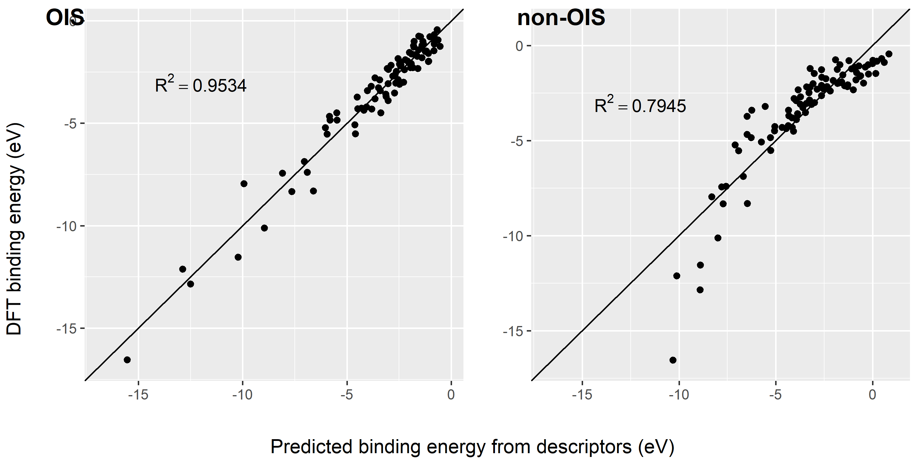
Figure 7: DFT binding energies versus predicted values using linear models with OIS and without OIS. The black line is $y=x$. Each model has $k=3$ descriptors.

5 Discussion

In this article, we study variable selection in the presence of feature engineering that is widely applicable in many scientific fields to provide interpretable models. Unlike in classical variable selection, candidate predictors are engineered from primary features and composite operators. While this problem has become increasingly important in science, such as the emerging field of materials informatics, the induced new geometry has not been studied in the statistical literature. We propose a new strategy “parametrics assisted by nonparametrics”, or PAN, to efficiently explore the descriptor space and achieve nonparametric dimension reduction for linear models. Using BART-G.SE as the nonparametric module, the proposed method iBART iteratively constructs and selects complex descriptors. Compared to one-shot descriptor construction approaches, iBART does not operate on an ultra-high dimensional descriptor space and thus substantially mitigates the “curse of dimensionality” and high correlations among descriptors. We introduce the OIS framework, define a PAN criterion, and assess iBART through the lens of this criterion. This sets a foundation for future research in interpretable model selection with feature engineering.

Other than the methodological contributions, we use extensive experiments to demonstrate appealing empirical features of iBART that may be crucial for practitioners. iBART automates the feature generating step; one-shot methods such as SISSO often require user intervention as otherwise they are not scalable to handle the overwhelmingly large descriptor space—this descriptor space increases double exponentially in the number of primary features and binary operators as a result of compositions. iBART has excellent scalability and leads to robust performance when the dimension of primary features increases to a level that renders existing methods computationally infeasible. Compared to SISSO, which is widely perceived as state-of-the-art in the field of materials genomes, our data application shows that iBART reduces the out-of-sample RMSE by 16% with an over 30-fold speedup and a fraction of memory demand. Overall, the proposed method accomplishes traditionally “server-required” tasks using a regular laptop or desktop with improved accuracy. Beyond materials genomes illustrated in Section 4, iBART can be applied to a vast domain where interpretable modeling is of interest.

There are interesting next directions building on our iBART approach. First, OIS provides a useful perspective for structured variable selection by introducing operators and compositions. Certain operator sets may be particularly useful depending on the application; for example, the composite multiply operator leads to high-order interactions. It is interesting to examine the performance of iBART with a diverse choice of operators. Also, we have focused on finite sample performance when assessing selection accuracy through simulations partly in view of the limited sample size typically available in the motivating example. It is nevertheless interesting to theoretically investigate the necessary conditions for the PAN criterion to hold for selected nonparametric variable selection methods such as BART when the sample size diverges.

References

- Bleich et al. (2014) Bleich, J., Kapelner, A., George, E. I. and Jensen, S. T. (2014) Variable selection for BART: an application to gene regulation. Annals of Applied Statistics, 8, 1750–1781.
- Chipman et al. (2010) Chipman, H. A., George, E. I. and McCulloch, R. E. (2010) BART: Bayesian additive regression trees. Annals of Applied Statistics, 4, 266–298.
- Fan and Lv (2008) Fan, J. and Lv, J. (2008) Sure independence screening for ultrahigh dimensional feature space. Journal of the Royal Statistical Society: Series B (Statistical Methodology), 70, 849–911.
- Feurer et al. (2015) Feurer, M., Klein, A., Eggensperger, K., Springenberg, J., Blum, M. and Hutter, F. (2015) Efficient and robust automated machine learning. In Advances in Neural Information Processing Systems, vol. 28. Curran Associates, Inc.
- Foppa et al. (2021) Foppa, L., Ghiringhelli, L. M., Girgsdies, F., Hashagen, M., Kube, P., Hävecker, M., Carey, S. J., Tarasov, A., Kraus, P., Rosowski, F., Schlögl, R., Trunschke, A. and Scheffler, M. (2021) Materials genes of heterogeneous catalysis from clean experiments and artificial intelligence. MRS Bulletin, 46, 1016–1026.
- Ghiringhelli et al. (2015) Ghiringhelli, L. M., Vybiral, J., Levchenko, S. V., Draxl, C. and Scheffler, M. (2015) Big data of materials science: Critical role of the descriptor. Phys. Rev. Lett., 114, 105503.
- Hart et al. (2021) Hart, G. L., Mueller, T., Toher, C. and Curtarolo, S. (2021) Machine learning for alloys. Nature Reviews Materials, 1–26.
- Horiguchi et al. (2021) Horiguchi, A., Pratola, M. T. and Santner, T. J. (2021) Assessing variable activity for bayesian regression trees. Reliability Engineering & System Safety, 207, 107391.
- Keith et al. (2021) Keith, J. A., Vassilev-Galindo, V., Cheng, B., Chmiela, S., Gastegger, M., Müller, K.-R. and Tkatchenko, A. (2021) Combining machine learning and computational chemistry for predictive insights into chemical systems. Chemical Reviews, 121, 9816–9872.
- Khurana et al. (2018) Khurana, U., Samulowitz, H. and Turaga, D. (2018) Feature engineering for predictive modeling using reinforcement learning. In The Thirty-Second AAAI Conference on Artificial Intelligence (AAAI-18).
- Lin et al. (2021) Lin, Y., Saboo, A., Frey, R., Sorkin, S., Gong, J., Olson, G. B., Li, M. and Niu, C. (2021) CALPHAD uncertainty quantification and TDBX. JOM, 73, 116–125.
- Linero (2018) Linero, A. R. (2018) Bayesian regression trees for high-dimensional prediction and variable selection. Journal of the American Statistical Association, 113, 626–636.
- Liu et al. (2022) Liu, C.-Y., Ye, S., Li, M. and Senftle, T. P. (2022) A rapid feature selection method for catalyst design: Iterative Bayesian additive regression trees (iBART). The Journal of Chemical Physics, 156, 164105.
- Liu et al. (2020) Liu, C.-Y., Zhang, S., Martinez, D., Li, M. and Senftle, T. P. (2020) Using statistical learning to predict interactions between single metal atoms and modified MgO(100) supports. npj Computational Materials, 6, 102.
- Liu et al. (2021a) Liu, X., Wu, Y., Irving, D. L. and Li, M. (2021a) Gaussian graphical models with graph constraints for magnetic moment interaction in high entropy alloys. ArXiv e-prints.
- Liu et al. (2021b) Liu, Y., Ročková, V. and Wang, Y. (2021b) Variable selection with ABC Bayesian forests. Journal of the Royal Statistical Society: Series B (Statistical Methodology), 83, 453–481.
- Markovitch and Rosenstein (2002) Markovitch, S. and Rosenstein, D. (2002) Feature generation using general constructor functions. Machine Learning, 49, 59–98.
- O’Connor et al. (2018) O’Connor, N. J., Jonayat, A. S. M., Janik, M. J. and Senftle, T. P. (2018) Interaction trends between single metal atoms and oxide supports identified with density functional theory and statistical learning. Nature Catalysis, 1, 531–539.
- Ouyang et al. (2018) Ouyang, R., Curtarolo, S., Ahmetcik, E., Scheffler, M. and Ghiringhelli, L. M. (2018) SISSO: A compressed-sensing method for identifying the best low-dimensional descriptor in an immensity of offered candidates. Physical Review Materials, 2, 083802.
- Tibshirani (1996) Tibshirani, R. (1996) Regression shrinkage and selection via the Lasso. Journal of the Royal Statistical Society: Series B (Methodological), 58, 267–288.
- Wang et al. (2018) Wang, A., Li, J. and Zhang, T. (2018) Heterogeneous single-atom catalysis. Nature Reviews Chemistry, 2, 65–81.
- Yang et al. (2013) Yang, X.-F., Wang, A., Qiao, B., Li, J., Liu, J. and Zhang, T. (2013) Single-atom catalysts: A new frontier in heterogeneous catalysis. Accounts of Chemical Research, 46, 1740–1748.
- Zhong et al. (2020) Zhong, M., Tran, K., Min, Y., Wang, C., Wang, Z., Dinh, C.-T., De Luna, P., Yu, Z., Rasouli, A. S., Brodersen, P., Sun, S., Voznyy, O., Tan, C.-S., Askerka, M., Che, F., Liu, M., Seifitokaldani, A., Pang, Y., Lo, S.-C., Ip, A., Ulissi, Z. and Sargent, E. H. (2020) Accelerated discovery of CO2 electrocatalysts using active machine learning. Nature, 581, 178–183.