Precision analysis of the redshift-space galaxy bispectrum

Abstract

We study the information content of the angle-averaged (monopole) redshift space galaxy bispectrum. The main novelty of our approach is the use of a systematic tree-level perturbation theory model that includes galaxy bias, IR resummation, and also accounts for nonlinear redshift space distortions, binning, and projection effects. We analyze data from the PT challenge simulations, whose cumulative volume of 566 $h^{-3}$Gpc³ allows for a precise comparison to theoretical predictions. Fitting the power spectrum and bispectrum of our simulated data, and varying all necessary cosmological and nuisance parameters in a consistent Markov chain Monte Carlo analysis, we find that our tree-level bispectrum model is valid up to $k_{\rm max}=0.08~{}h\text{Mpc}^{-1}$ (at $z=0.61$). We also find that inclusion of the bispectrum monopole improves constraints on cosmological parameters by $(5-15)\%$ relative to the power spectrum. The improvement is more significant for the quadratic bias parameters of our simulated galaxies, which we also show to deviate from biases of the host dark matter halos at the $\sim 3\sigma$ level. Finally, we adjust the covariance and scale cuts to match the volume of the BOSS survey, and estimate that within the minimal $\Lambda$CDM model the bispectrum data can tighten the constraint on the mass fluctuation amplitude $\sigma_{8}$ by roughly $10\%$.

YITP-21-120, CERN-TH-2021-155

1 Introduction

The three-point function, or its Fourier transform the bispectrum [1], is the simplest statistic beyond the power spectrum that captures information about the large-scale spatial distribution of galaxies. The shape dependence of the bispectrum is sensitive to cosmological initial conditions, gravitational instability, and galaxy formation physics. For this reason the bispectrum is an important observational probe which can improve our understanding of both galaxy formation and fundamental cosmology [2, 3]. It has been argued that it may help sharpen the limits on conventional cosmological parameters [3, 4, 5, 6], neutrino masses [6, 7, 8], and primordial non-Gaussianity [9, 4, 10]. While these results are encouraging, they are often based on idealized Fisher forecasts and overoptimistic assumptions about the validity of theoretical models needed to describe the data. Therefore, it is still not clear whether the inclusion of the bispectrum will be worth the effort, whether it will really make a difference in a realistic analysis where all relevant cosmological and nuisance parameters are varied.

A quantitative answer to this question cannot be given without performing a consistent data analysis. While the three-point functions and bispectra of the galaxy density field have been measured both in simulations and in a number of past and current datasets (e.g. Zwicky and Lick catalogs [11, 12], IRAS [13, 14], WiggleZ [15], Baryon Oscillation Spectroscopic Survey (BOSS) [16, 17, 18, 19]), the proper cosmological analyses of the bispectrum are still lacking. This is clearly in sharp contrast with the galaxy power spectrum analyses, which have been routinely used as an important source of information on cosmological parameters. There are multiple factors that make the bispectrum analysis much more challenging.

From the computational side, the main challenge is a large number of data points, which correspond to triangle configurations formed by three wavevectors ${\bf k}_{1},{\bf k}_{2},{\bf k}_{3}$. Typical bispectra datasets consist of hundreds of triangles, which makes it hard to estimate the bispectrum from catalogs, compute the covariance matrix, and perform likelihood analysis. This stimulated the development of fast estimators [20, 21, 22, 23, 24], various compression techniques [2, 25, 26, 27] and efficient mock catalog pipelines [28].

From the theory side, the main challenge is modeling non-linear effects of matter clustering, galaxy bias, and redshift space distortions. Recent analyses described these effects by means of N-body simulations, which were used to calibrate phenomenological bispectrum models [29, 16, 17, 18, 30]. This simulation-based approach naturally extends to ‘emulation’, in which the data is fitted directly to the simulation output [31, 32, 33, 7, 8]. Despite significant progress in numerical modeling of galaxy clustering over last years, it is not yet clear if emulators can meet precision requirements of future surveys, see e.g. [34]. The main issue is persistent uncertainty in galaxy formation physics, which has to be marginalized over in order to obtain robust cosmological constraints. This motivates the development of more conservative perturbative techniques [35, 36, 37, 38], which have recently taken non-linear large-scale structure modeling to a new precision level by virtue of the progress in the effective field theory (EFT) of large-scale structure [39, 40].

Unlike simulation-based approaches, EFT is fundamentally restricted to scales larger than $2\pi k_{\rm NL}^{-1}\sim 10$ Mpc. However, in the regime where it is applicable, EFT allows calculations to arbitrary order, and hence it provides a program of systematic successive approximations to the true answer. Moreover, by construction, EFT covers all possible galaxy formation scenarios by means of “nuisance parameters,” which fully capture the impact of galaxy evolution on large scale clustering. Thus, this framework is naturally designed for the marginalization over galaxy formation physics, which boils down to a literal marginalization over nuisance parameters. Finally, EFT-based theoretical templates for a given cosmological model can be quickly generated with modifications of Boltzmann codes, e.g. [41, 42, 43], which allow one to efficiently explore the cosmology-dependence of large-scale structure data.

The full utility of the EFT approach has been shown recently in the analysis of the galaxy power spectrum data from BOSS [44]. This has resulted in first-ever measurements of fundamental cosmological parameters, such as the Hubble constant and the amplitude of the primordial scalar fluctuations, from the full shape of the galaxy power spectrum [45, 46]. Moreover, the EFT-based full shape analyses have opened up a new opportunity to testing beyond-$\Lambda$CDM scenarios in a rigorous and self-consistent fashion [47, 48, 42, 49, 50].

An important step in applying the EFT calculations to the real data was the validation of the EFT-based power spectrum likelihoods on high-fidelity simulations [45, 46, 51, 50]. In particular, the EFT-based pipelines have passed a blind test on galaxy mock catalogs called “PT challenge” [52]. The PT challenge simulation suite covers a cumulative volume of $566~{}h^{-3}$Gpc³, which is significantly larger than the volume of current and planned surveys. This large volume is chosen with the purpose of dramatically reducing statistical error and thereby identifying systematic uncertainties in theoretical modeling at the unprecedented sub-percent level.

Inspired by the success of the EFT approach in the power spectrum analysis, in this work we extend the study of the PT challenge simulation data from Ref. [52] to the galaxy bispectrum. We analyze this data with the currently available tree-level EFT model. The two main goals of our work are (a) to define the validity range of this model and to (b) assess the information content of the redshift-space galaxy bispectrum in the tree-level approximation. Achieving these goals will bring us one step closer to understanding the information content of the galaxy bispectrum and building a pipeline that can be used to analyze real data.

The paper is structured as follows. We describe the PT challenge simulations in Section 2. Section 3 describes in detail our theoretical model. In Section 4 we discuss our baseline power spectrum and bispectrum likelihoods. Our main results are presented in Section 5, where we analyze the real space and redshift space monopole bispectrum data in combination with the baseline redshift space power spectrum likelihood. We discuss improvements in cosmological and bias parameters and give a forecast for a BOSS-like survey. There we also compare the measured values of galaxy bias parameters with those expected from dark matter halo relations. We compare our analysis with previous works in Section 6 and draw conclusions in Section 7. Several appendices contain additional material and tests. In Appendix A we validate our binning approach, and in Appendix B we show that “open” triangles do not carry any significant cosmological information. In Appendix C we test our covariance matrix choices. Our baseline power spectrum likelihood is described in Appendix D. Appendix E contains an analysis of the power spectrum and bispectrum purely in real space. Theoretical calculations of the power spectrum and bispectrum covariance matrices in perturbation theory are presented in Appendix F, while Appendix G contains a derivation of the Gaussian fingers-of-God damping.

2 Data

The PT challenge simulation suite consists of 10 boxes, each with the side length $L=3840~{}h^{-1}$Mpc. The gravitational evolution was traced by 3072³ particles in each box. In this paper we consider one particular snapshot taken at $z=0.61$, which corresponds to the BOSS CMASS1 sample [44]. The dark matter halos from this snapshot were populated with mock CMASS-like red luminous galaxies following the halo occupation distribution (HOD) prescription detailed in Ref. [52]. We refer the reader to this reference for further details on the simulations. The redshift-space power spectrum multipoles $\ell=0,2,4$ were estimated as

$$\hat{P}_{\ell}(k_{i})=\frac{2\ell+1}{N_{i}}\sum_{\tilde{\bf k}\in k_{i}}\mathcal{L}_{\ell}(\mu_{\tilde{\bf k}})\hat{P}(\tilde{\bf k})\,,$$ (2.1)

where we have introduced

$$\hat{P}(\tilde{\bf k})=\frac{\tilde{V}|\delta_{\tilde{\bf k}}|^{2}-\bar{n}^{-1}}{W^{2}_{\rm CIC}(\tilde{\bf k})}\,,\quad\tilde{V}=\left(\frac{D_{A}^{(\rm fid)}(z)}{D_{A}^{(\rm true)}(z)}\right)^{2}\frac{H^{(\rm true)}(z)}{H^{(\rm fid)}(z)}L^{3}\,,$$ (2.2)

and $\delta_{\tilde{\bf k}}$ is the Fourier space overdensity field, the sum runs over all modes whose norms belong to a bin $[(i-1)\Delta k,i\Delta k]$, we use $\Delta k=0.01~{}h\text{Mpc}^{-1}$ and $N_{i}$ is the number of Fourier modes in the bin. The modes in the sum in Eq. (2.1) are composed of fundamental modes $k_{f}=2\pi L^{-1}$, which were rescaled by the Alcock-Paczynski (AP) effect [72] as,

$$\tilde{k}_{f,x}=k_{f,x}\frac{D_{A}^{(\rm true)}(z)}{D_{A}^{(\rm fid)}(z)}\,,\quad\tilde{k}_{f,y}=k_{f,y}\frac{D_{A}^{(\rm true)}(z)}{D_{A}^{(\rm fid)}(z)}\,,\quad\tilde{k}_{f,z}=k_{f,z}\frac{H^{(\rm fid)}(z)}{H^{(\rm true)}(z)}\,,$$ (2.3)

where the upper scripts (true) and (fid) denote the comoving angular diameter distance $D_{A}(z)$ and the Hubble parameter $H(z)$ calculated in the true and fiducial cosmologies, respectively. The fiducial cosmological model is the same as in Ref. [52], flat $\Lambda$CDM with $\Omega_{m}^{(\rm fid)}=0.3$. Note that we have subtracted the Poissonian shot noise power spectrum contribution

$$\frac{1}{\bar{n}}=\frac{L^{3}}{N_{\rm gal}}\,,$$ (2.4)

where $N_{\rm gal}$ is the total number of galaxies, taking into account the interlacing technique for the aliasing correction and the CIC window function. If not stated otherwise, we will be using the datavector $[P_{0},P_{2},P_{4}]$ with $k_{\rm max}=0.14~{}h\text{Mpc}^{-1}$. In addition, we employ the transverse moment $Q_{0}$ (equivalent of the real space power spectrum), which is estimated from the redshift space multipoles via

$$\hat{Q}_{0}=\hat{P}_{0}-\frac{1}{2}\hat{P}_{2}+\frac{3}{8}\hat{P}_{4}\,,$$ (2.5)

see Refs. [73] for more detail and also Refs. [74, 75, 76] for earlier works. We use $Q_{0}$ in the range of scales

$$0.14~{}h\text{Mpc}^{-1}\leq k<0.4~{}h\text{Mpc}^{-1}\,,$$

so that it is not correlated with the multipoles’ datavector.

The angle-averaged (monopole) bispectrum is computed using the following estimator:

$$\hat{B}_{0}(k_{1},k_{2},k_{3})=\frac{1}{N_{B}(k_{1},k_{2},k_{3})}\sum_{\tilde{\bf q}_{1}\in k_{1}}\sum_{\tilde{\bf q}_{2}\in k_{2}}\sum_{\tilde{\bf q}_{3}\in k_{3}}\delta_{\rm K}(\tilde{\bf q}_{123})\delta_{\tilde{\bf q}_{1}}\delta_{\tilde{\bf q}_{2}}\delta_{\tilde{\bf q}_{3}}\,,$$ (2.6)

where $\tilde{\bf q}_{123}\equiv\tilde{\bf q}_{1}+\tilde{\bf q}_{2}+\tilde{\bf q}_{3}$, and $\delta_{\rm K}({\bf q}_{123})$ denotes the Kronecker delta function,

$$\delta_{K}({\bf q}_{123})=\begin{cases}1,&\text{if ${\bf q}_{123}=0$}.\\ 0,&\text{otherwise},\end{cases}$$ (2.7)

and $N_{B}(k_{1},k_{2},k_{3})$ is the number of fundamental triangles in the bin defined by wavenumber centers $(k_{1},k_{2},k_{3})$. Each bin has width $\Delta k=0.01~{}h\text{Mpc}^{-1}$, which is the same as for the power spectrum estimator. Note that unlike the power spectrum, we do not subtract the shot noise contributions from the bispectrum. The estimator Eq. (2.6) is evaluated with FFTs using the Scoccimarro method [20].

The real space bispectrum is calculated using the same formula Eq. (2.6), but with the real space density $\delta^{\rm real}_{\bf k}$ and without the AP effect.

3 Theory Model

Let us describe our theoretical model for the redshift space bispectrum. We will discuss each relevant component separately.

In what follows we will work in the plane-parallel approximation. The galaxy density contrast field in redshift space at quadratic order in perturbation theory reads [62, 68]

$$\begin{split}\delta^{(z)}({\bf k})=&Z_{1}({\bf k})\delta^{(1)}({\bf k})+[Z_{2}(\delta^{(1)})^{2}]_{\bf k}+d_{1}\epsilon({\bf k})\,,\\ &+d_{2}b_{1}\delta^{(1)}({\bf k})\epsilon({\bf k})+(d_{1}\epsilon({\bf k}))f\mu^{2}\theta^{(1)}({\bf k})+...\,,\end{split}$$ (3.1)

where $\delta^{(1)},\theta^{(1)}$ are linear matter density and velocity divergence fields (satisfying $\theta^{(1)}=\delta^{(1)}$); $\epsilon$ is the stochastic galaxy overdensity field, $d_{1},d_{2}$ are free parameters, and the standard perturbation theory [77] kernels are given by:

$$Z_{1}({\bf k})=b_{1}+f\mu^{2}\,,$$ (3.2a)

$$Z_{2}({\bf k}_{1},{\bf k}_{2})=\frac{b_{2}}{2}+b_{\mathcal{G}_{2}}\left(\frac{({\bf k}_{1}\cdot{\bf k}_{2})^{2}}{k_{1}^{2}k_{2}^{2}}-1\right)+b_{1}F_{2}({\bf k}_{1},{\bf k}_{2})+f\mu^{2}G_{2}({\bf k}_{1},{\bf k}_{2})$$

$$\qquad\qquad\quad~{}~{}+\frac{f\mu k}{2}\left(\frac{\mu_{1}}{k_{1}}(b_{1}+f\mu_{2}^{2})+\frac{\mu_{2}}{k_{2}}(b_{1}+f\mu_{1}^{2})\right)\,,$$ (3.2b)

$$F_{2}({\bf k}_{1},{\bf k}_{2})=\frac{5}{7}+\frac{1}{2}\left(\frac{({\bf k}_{1}\cdot{\bf k}_{2})}{k_{1}^{2}}+\frac{({\bf k}_{1}\cdot{\bf k}_{2})}{k_{2}^{2}}\right)+\frac{2}{7}\frac{({\bf k}_{1}\cdot{\bf k}_{2})^{2}}{k_{1}^{2}k_{2}^{2}}\,,$$ (3.2c)

$$G_{2}({\bf k}_{1},{\bf k}_{2})=\frac{3}{7}+\frac{1}{2}\left(\frac{({\bf k}_{1}\cdot{\bf k}_{2})}{k_{1}^{2}}+\frac{({\bf k}_{1}\cdot{\bf k}_{2})}{k_{2}^{2}}\right)+\frac{4}{7}\frac{({\bf k}_{1}\cdot{\bf k}_{2})^{2}}{k_{1}^{2}k_{2}^{2}}\,,$$ (3.2d)

where $\mu_{i}\equiv({\bf k}_{i}\cdot\hat{{\bf z}})/k_{i}$, $\mu\equiv({\bf k}\cdot\hat{{\bf z}})/k$, ${\bf k}\equiv{\bf k}_{1}+{\bf k}_{2}$, and $f$ is the logarithmic growth factor, related to the usual linear growth rate $D_{+}$ via

$$f=\frac{d\mathop{\rm ln}\nolimits D_{+}}{d\mathop{\rm ln}\nolimits a}\,,$$ (3.3)

with $a$ being the scale factor in the Friedmann metric. The coefficients $b_{1}$, $b_{2}$, and $b_{\mathcal{G}_{2}}$ capture linear, quadratic, and tidal bias between matter and galaxies, respectively. The tree-level bispectrum is obtained by computing the three-point function of the perturbative density field at second order [67],

$$\begin{split}&B_{\rm ggg}({\bf k}_{1},{\bf k}_{2},{\bf k}_{3})=~{}2Z_{2}({\bf k}_{1},{\bf k}_{2})Z_{1}({\bf k}_{1})Z_{1}({\bf k}_{2})P_{\rm lin}(k_{1})P_{\rm lin}(k_{2})\\ &+P_{\epsilon}(k_{2})2d_{1}\left(d_{2}b_{1}+d_{1}f\mu^{2}_{1}\right)Z_{1}({\bf k}_{1})P_{\rm lin}(k_{1})+\text{cycl.}+d_{1}^{3}B_{\epsilon}({\bf k}_{1},{\bf k}_{2},{\bf k}_{3})\,,\end{split}$$ (3.4)

where we have used the following correlation functions

$$\begin{split}&\langle\delta^{(1)}({\bf k})\delta^{(1)}({\bf k}^{\prime})\rangle=(2\pi)^{3}\delta^{(3)}_{D}({\bf k}+{\bf k}^{\prime})P_{\rm lin}(k)\,,\\ &\langle\epsilon({\bf k})\epsilon({\bf k}^{\prime})\rangle=(2\pi)^{3}\delta^{(3)}_{D}({\bf k}+{\bf k}^{\prime})P_{\epsilon}(k)\\ &\langle\epsilon({\bf k}_{1})\epsilon({\bf k}_{2})\epsilon({\bf k}_{3})\rangle=(2\pi)^{3}\delta^{(3)}_{D}({\bf k}_{1}+{\bf k}_{2}+{\bf k}_{3})B_{\epsilon}({\bf k}_{1},{\bf k}_{2},{\bf k}_{3})\,.\end{split}$$ (3.5)

Stochastic terms.

At quadratic order in perturbation theory the shot-noise contributions are constants,

$$P_{\epsilon}=\text{const}\,,\quad B_{\epsilon}=\text{const}\,.$$ (3.6)

Furthermore, if $\epsilon$ is Poisson-distributed, both statistics are fully determined by the galaxy number density $\bar{n}$ (see e.g. Ref. [78] and references therein):

$$B_{\epsilon}=P_{\epsilon}^{2}=\frac{1}{\bar{n}^{2}}\,.$$ (3.7)

However, due to halo exclusion, deviations from Poissonian sampling are known to be important [79, 80, 81, 82], in which case we cannot use Eq. (3.7) and the tree-level bispectrum should be characterized by three free parameters capturing stochasticity. We define them to be $P_{\rm shot},B_{\rm shot}$ and $A_{\rm shot}$;

$$\begin{split}d_{1}^{2}\langle\epsilon^{2}\rangle=\frac{1+P_{\rm shot}}{\bar{n}}\,,\quad d_{1}^{3}\langle\epsilon^{3}\rangle=\frac{A_{\rm shot}}{\bar{n}^{2}}\,,\quad B_{\rm shot}\equiv 2d_{2}d^{-1}_{1}\left(1+P_{\rm shot}\right)\,,\end{split}$$ (3.8)

which are expected to be $\mathcal{O}(1)$ numbers. Importantly, the parameter $P_{\rm shot}$ also enters the power spectrum model. Furthermore, following [64, 16, 46] we will assume that the bispectrum and power spectrum of the stochastic overdensity component are correlated as in the Poissonian case (3.7), but their values are different from $\bar{n}^{-1}$, i.e.

$$B_{\epsilon}=P_{\epsilon}^{2}\,,\quad\Rightarrow\quad A_{\rm shot}=(1+P_{\rm shot})^{2}\,,$$ (3.9)

which is ultimately motivated by the expectation that departures from the Poissonian sampling are small. We have found that the bispectrum data is fully consistent with this hypothesis. Therefore, we adopt this choice as our baseline model for the stochastic nuisance parameters, which helps us reduce their number down to two.

Fingers-of-God.

An important feature of non-linear redshift-space distortions is the sensitivity to the stochastic velocity field, which can have relatively large scale correlations due to halo virialization [76]. This effect is called “fingers-of-God” (FoG) [83]. In the EFT, FoG are captured perturbatively through the gradient expansion involving derivatives along the line-of-sight [60, 61, 62, 84, 85, 43]. These corrections are called “counterterms,” and at leading one-loop order they are given by [62]

$$\delta^{\rm ctr.}=-c_{0}\left(\frac{k}{k_{\rm NL}}\right)^{2}-(c_{1}\mu^{2}+c_{2}\mu^{4})\left(\frac{k}{k^{r}_{\rm NL}}\right)^{2}\,.$$ (3.10)

The role of $\mu$-dependent counterterm coefficients $c_{1}$ and $c_{2}$ is to capture the physical impact of the FoG on large scale fluctuations. In principle, the FoG is a one-loop effect in the EFT nomenclature, and it needs to be included along with other, “standard,” one-loop corrections, which we ignore in this work. The characteristic momentum scale of these one-loop corrections matches the real space dark matter cutoff $k_{\rm NL}$. If $2\pi/k^{r}_{\rm NL}$ is larger than $2\pi k^{-1}_{\rm NL}$ (and the cutoff of the bias expansion $2\pi k^{-1}_{\rm M}$), the FoG counterterm can actually dominate over usual loop corrections. This is the exact situation that was observed for matter and galaxy power spectra in redshift space, where FoG corrections were found to be important even on relatively large scales where the “standard” loop corrections (i.e. without the counterterms) are suppressed [61, 45, 52, 51, 86].

This motivates including the FoG counterterms $c_{1},c_{2}$ in our theory model even though formally they capture one-loop effects. Another rationale behind this practice is that these counterterms can be treated as a proxy for the theoretical error [4, 51]. This will also serve us as a tool to check if the tree-level calculation can be trusted: if the counterterm contribution dominates the tree-level bispectrum signal, the one-loop corrections cannot be ignored anymore.

In practice, we have found that it is sufficient to include only the $k^{2}\mu^{2}$ counterterm in our theory model. We ignore the contribution $k^{2}\mu^{4}$ because we have found that it is very degenerate with the $k^{2}\mu^{2}$ shape at the level of the bispectrum monopole, and hence we set $c_{2}=0$ in what follows. Note that we will have to include both $c_{1}$ and $c_{2}$ when we consider higher order angular multipole moments. The inclusion of the $c_{1}$ counterterm amounts to correcting the kernel $Z_{1}$ as

$$Z_{1}\to Z^{\rm FoG}_{1}=b_{1}+f\mu^{2}-c_{1}\mu^{2}\left(\frac{k}{k^{r}_{\rm NL}}\right)^{2}\,.$$ (3.11)

In what follows we set $k_{\rm NL}^{r}=0.3~{}h\text{Mpc}^{-1}$ in agreement with the measurement of the cutoff for the Red Luminous Galaxies from the power spectrum of the PT challenge mocks [52, 86].

IR resummation.

Naive attempts to build the EFT as a perturbative expansion in terms of smoothed (large-scale) density and velocity fields break down for the BAO part of the linear power spectrum (sometimes loosely referred to as the “BAO wiggles”). The procedure of resumming enhanced perturbative (loop) corrections to this part of the spectrum is called “IR resummation” [87, 88, 89, 90, 91, 69] (see Refs. [92, 92] for earlier works). IR resummation effects have to be included in the theory model even when it is evaluated at the tree level [88, 69]. IR-resummation for the bispectrum in redshift space has been calculated in Ref. [70] (see Ref. [93] for IR resummation of the bispectrum in the case of non-Gaussian initial conditions). At leading order this procedure amounts to the replacement of the linear matter power spectrum by its resummed version,

$$P_{\rm lin}(k)\to P^{\rm IR-res}_{\rm tree}(k)=P_{\rm nw}(k)+P_{\rm w}(k){\rm e}^{-\Sigma^{2}k^{2}(1+f\mu^{2}(2+f))-\delta\Sigma^{2}k^{2}f^{2}\mu^{2}(\mu^{2}-1)}\,,$$ (3.12)

where $P_{\rm w}$ is the part of the spectrum that contains the BAO wiggles, $P_{\rm nw}\equiv P_{\rm lin}-P_{\rm w}$,

$$\begin{split}&\Sigma^{2}=\frac{1}{6\pi^{2}}\int_{0}^{k_{S}}dq~{}P_{\rm nw}(q)(1-j_{0}(qr_{\rm BAO})+2j_{2}(qr_{\rm BAO}))\,,\\ &\delta\Sigma^{2}=\frac{1}{2\pi^{2}}\int_{0}^{k_{S}}dq~{}P_{\rm nw}(q)j_{2}(qr_{\rm BAO})\,,\end{split}$$ (3.13)

are the BAO damping functions, $j_{\ell}(x)$ are spherical Bessel functions, $r_{\rm BAO}$ is the comoving sound horizon at the drag epoch, $k_{S}$ is the separation scale defining IR modes that need to be resummed. In practice we use $k_{S}=0.05~{}h/$Mpc following Ref. [69], although other choices, e.g. $k_{S}=k/2$ [88] give statistically indistinguishable results.

All in all, our final tree-level bispectrum model reads (c.f. [68]):

$$\begin{split}B_{\rm ggg}=&\left[~{}2Z_{2}({\bf k}_{1},{\bf k}_{2})Z^{\rm FoG}_{1}({\bf k}_{1})Z^{\rm FoG}_{1}({\bf k}_{2})P^{\rm IR-res}_{\rm tree}({\bf k}_{1})P^{\rm IR-res}_{\rm tree}({\bf k}_{2})\right.\\ &\left.+\frac{B_{\rm shot}}{\bar{n}}\left(b_{1}+2\frac{1+P_{\rm shot}}{B_{\rm shot}}f\mu^{2}\right)Z^{\rm FoG}_{1}({\bf k}_{1})P^{\rm IR-res}_{\rm tree}({\bf k}_{1})+\text{cycl.}\right]+\frac{(1+P_{\rm shot})^{2}}{\bar{n}^{2}}\,,\end{split}$$ (3.14)

where $b_{1}$, $b_{2}$, $b_{\mathcal{G}_{2}}$, $P_{\rm shot},B_{\rm shot}$ are nuisance parameters to marginalize over. Note that $B_{\rm shot}$ is the only new parameter that is not present in the power spectrum model.

Redshift space multipoles.

In real space the bispectrum depends on three kinematic variables (wavelengths) which characterize the shape of a triangle. In redshift space there appears an additional dependence due to the orientation of the triangle w.r.t. the line-of-sight direction. This orientation is characterized by two angles, which we choose, following Ref. [38], to be the polar angle of ${\bf k}_{1}$ (its cosine is $\cos\theta=\mu\equiv(\hat{{\bf k}}_{1}\cdot\hat{{\bf z}})$) and the azimuthal angle around ${\bf k}_{1}$ denoted by $\phi$. In this case the angles between wavevectors ${\bf k}_{a}$ (a=1,2,3) and the line-of-sight are given by

$$\begin{split}&\mu_{1}=\mu\,,\\ &\mu_{2}=\mu\cos\alpha-(1-\mu^{2})^{1/2}\sin\alpha\cos\phi\,,\\ &\mu_{3}=-\frac{k_{1}}{k_{3}}\mu-\frac{k_{2}}{k_{3}}\mu_{2}\,,\end{split}$$ (3.15)

where $\cos\alpha=x=(\hat{{\bf k}}_{1}\cdot\hat{{\bf k}}_{2})$. It is convenient to describe this angular dependence by expanding $B_{\rm ggg}$ in spherical harmonics,

$$\begin{split}&B_{\rm ggg}({\bf k}_{1},{\bf k}_{2},{\bf k}_{3})=\sum_{\ell=0}^{\infty}\sum_{m=-\ell}^{\ell}B_{\ell m}(k_{1},k_{2},k_{3})Y_{\ell m}(\theta,\phi)\,,\\ &B_{\ell m}(k_{1},k_{2},k_{3})=\frac{2\ell+1}{2}\int_{0}^{2\pi}d\phi\int_{-1}^{1}d(\cos\theta)~{}Y^{*}_{\ell m}(\theta,\phi)~{}B_{\rm ggg}({\bf k}_{1},{\bf k}_{2},{\bf k}_{3})\,.\end{split}$$ (3.16)

In what follows we will focus on the $m=0$ sector [20]. The corresponding momenta $B_{\ell}$ are called “bispectrum multipoles,”

$$\begin{split}B_{\ell}(k_{1},k_{2},k_{3})=\frac{2\ell+1}{2}\int_{0}^{2\pi}\frac{d\phi}{2\pi}\int_{-1}^{1}d(\cos\theta)~{}\mathcal{L}_{\ell}(\cos\theta)~{}B_{\rm ggg}({\bf k}_{1},{\bf k}_{2},{\bf k}_{3})\,,\end{split}$$ (3.17)

where $\mathcal{L}_{\ell}$ denotes a Legendre polynomial of order $\ell$. Note that the integral above can be done analytically at the tree level in the absence of IR resummation and the AP effect [38]. However, in what follows we will use the full formula (3.14) with IR resummation, and evaluate angular integrals in Eq. (3.17) numerically via Gauss-Legendre quadrature.

Alcock-Paczynski effect.

The AP conversion [72] from true wavenumbers and angles ($q,\nu$) to observed wavenumbers and angles $(k,\mu)$ is given by

$$\begin{split}q^{2}&=k^{2}\left[\alpha_{\parallel}^{-2}\mu^{2}+\alpha_{\perp}^{-2}(1-\mu^{2})\right]\,,\\ \nu^{2}&=\alpha_{\parallel}^{-2}\mu^{2}\left[\alpha_{\parallel}^{-2}\mu^{2}+\alpha_{\perp}^{-2}(1-\mu^{2})\right]^{-1}\,,\end{split}$$ (3.18)

which depends on the ratios between the true and fiducial Hubble parameters and angular diameter distances at the redshift of interest,

$$\alpha_{\parallel}=\frac{H_{\rm fid}(z)}{H_{\rm true}(z)}\frac{H_{0,\rm true}}{H_{0,\rm fid}}\,,\quad\alpha_{\perp}=\frac{D_{\rm true,A}(z)}{D_{\rm fid,A}(z)}\frac{H_{0,\rm true}}{H_{0,\rm fid}}\,,$$ (3.19)

where additional factors $H_{0,\rm true}/H_{0,\rm fid}$ account for the fact that wavenumbers are measured in $h\text{Mpc}^{-1}$ units in our analysis. The observed power spectrum multipoles are given by [41]

$$P_{\ell}(k)=\frac{2\ell+1}{2\alpha^{2}_{\perp}\alpha_{\parallel}}\int_{-1}^{1}d\mu~{}\mathcal{L}_{\ell}(\mu)P_{\rm gg}(q[k,\mu],\nu[\mu])\,.$$ (3.20)

In full analogy, the bispectrum multipoles are given by [94]

$$\begin{split}&B_{\ell}(k_{1},k_{2},k_{3})\\ &=\frac{2\ell+1}{2\alpha^{2}_{\parallel}\alpha^{4}_{\perp}}\int_{0}^{2\pi}\frac{d\phi}{2\pi}\int_{-1}^{1}d\mu_{1}~{}\mathcal{L}_{\ell}(\mu_{1})~{}B_{\rm ggg}(q_{1}[k_{1},\mu_{1}],q_{2}[...],q_{3}[...],\nu_{1}[\mu_{1}],\nu_{2}[\mu_{2}(\mu_{1})])\,,\end{split}$$ (3.21)

where the observed angles satisfy Eq. (3.15). In what follows we will focus on the monopole moment $\ell=0$, and leave the analysis of other multipoles for future work.

Binning effects.

The measured bispectrum is a discrete approximation to a continuous Fourier-space field. In order to account for this discreteness we need to bin our theory predictions in the same way as we bin the data. Binning corrections are marginally important for the PT challenge power spectrum and it is straightforward to take them into account [52]. However, the situation is somewhat different for the bispectrum, where binning can be a serious source of systematics [95]. The exact discrete bispectrum that we extract from simulations is given by

$$\begin{split}&\hat{B}_{0,\rm disc}(k_{1},k_{2},k_{3})=\frac{\sum_{{\bf q}_{1}\in k_{1}}\sum_{{\bf q}_{2}\in k_{2}}\sum_{{\bf q}_{3}\in k_{3}}B({\bf q}_{1},{\bf q}_{2},{\bf q}_{3})\delta_{\rm K}({\bf q}_{123})}{N^{\rm disc}_{B}(k_{1},k_{2},k_{3})}\,,\\ &N^{\rm disc}_{B}(k_{1},k_{2},k_{3})=\sum_{{\bf q}_{1}\in k_{1}}\sum_{{\bf q}_{2}\in k_{2}}\sum_{{\bf q}_{3}\in k_{3}}\delta_{\rm K}({\bf q}_{123})\,.\end{split}$$ (3.22)

The sum in Eq. (3.22) runs over all discrete wavevectors ${\bf q}_{i}$ that belong to the triangle bin defined by its center $(k_{1},k_{2},k_{3})$ and width $\Delta k$. $N^{\rm disc}_{B}(k_{1},k_{2},k_{3})$ is the total number of these “fundamental triangles” inside the triangle bin $(k_{1},k_{2},k_{3})$ [96].

Before going into technical details, let us outline our strategy. As a first step, we take the continuum limit, i.e. assume a vanishingly small fundamental wavenumber $k_{f}=(2\pi)L^{-1}$ as a leading approximation. In this first approximation the discreetness effects can be taken into account by integrating the continuous bispectrum field within appropriate bins. It is natural to refer to this program as the “integral approximation.” Because the actual fundamental bin is finite, the integral approximation requires certain corrections. As a second step, we will introduce these corrections, which will be referred to as “discreetness weights.”

Note that with our binning scheme there are so-called “open” triangle bins. The centers of these bins $(k_{1},k_{2},k_{3})$ do not satisfy momentum conservation constraints, such as $|k_{3}-k_{2}|<k_{1}<k_{3}+k_{2}$. In what follows we will discard these triangles because of three reasons:

• their properties (and very existence) crucially depend on the box size, which makes it hard to make generic statements that would not depend on a particular survey volume;

• the leading binning effect cannot be well captured by the integral approximation for these triangles, and hence it requires a significant modification of our baseline binning program;

• these triangles do not carry any sizable cosmological information (at least at the level of the tree-level bispectrum likelihood) and with our particular choice of bins’ width), see Appendix B.

As a first step of our binning procedure we implement the integral approximation. Other binning schemes were explored in Refs. [97, 96, 98]. The integral approximation amounts to replacing the sum over the modes with the Fourier integral,

$$\begin{split}&\sum_{{\bf q}_{1}\in k_{1}}\sum_{{\bf q}_{2}\in k_{2}}\sum_{{\bf q}_{1}\in k_{2}}\delta_{\rm K}({\bf q}_{123})B({\bf q}_{1},{\bf q}_{2},{\bf q}_{3})\to\frac{V^{2}}{(2\pi)^{6}}\int_{{\bf k}_{1}{\bf k}_{2}{\bf k}_{3}}~{}(2\pi)^{3}\delta^{(3)}_{D}({\bf q}_{123})B({\bf q}_{1},{\bf q}_{2},{\bf q}_{3})\,,\\ &\sum_{{\bf q}_{1}\in k_{1}}\sum_{{\bf q}_{2}\in k_{2}}\sum_{{\bf q}_{1}\in k_{2}}\delta_{\rm K}({\bf q}_{123})\to\frac{V^{2}}{(2\pi)^{6}}\int_{{\bf k}_{1}{\bf k}_{2}{\bf k}_{3}}~{}(2\pi)^{3}\delta^{(3)}_{D}({\bf q}_{123})\end{split}$$ (3.23)

where $V$ is the box volume and we introduced

$$\begin{split}&\int_{{\bf k}_{1}{\bf k}_{2}{\bf k}_{3}}\equiv\int_{V_{k_{1}k_{2}k_{3}}}\frac{d^{3}q_{1}}{(2\pi)^{3}}\frac{d^{3}q_{2}}{(2\pi)^{3}}\frac{d^{3}q_{3}}{(2\pi)^{3}}\,,\quad V_{k_{1}k_{2}k_{3}}=\mathcal{D}_{1}\times\mathcal{D}_{2}\times\mathcal{D}_{3}\,,\\ &\mathcal{D}_{a}=\left\{(q_{x_{1}},q_{x_{2}},q_{x_{3}})\in\mathbb{R}^{3}:k_{a}-\frac{\Delta k}{2}\leq|{\bf q}_{a}|\leq k_{a}+\frac{\Delta k}{2}\right\}\,,\quad a=1,2,3\,.\end{split}$$ (3.24)

Figure 1: Upper left panel: the ratio between the number of fundamental triangles from the data and from the integral approximation, $N_{B}^{\rm disc.}/N_{123}$, as a function of the triangle bin. Upper right panel: the ratio between the exact binned bispectrum and the integral approximation (“discreteness weights” $w_{i}$), as a function of $N_{B}^{\rm disc.}/N_{123}$ for the same triangle bins. The triangles shown correspond to $k_{\rm max}=0.15~{}h/$Mpc. Lower panel: discreteness weights for folded triangles denoted by their bin centers (we use $\Delta k=0.01~{}h\text{Mpc}^{-1}$, and hence $k_{\rm min}=\Delta k/2=5\cdot 10^{-3}~{}h\text{Mpc}^{-1}$).

This way we arrive at

$$\begin{split}&\hat{B}_{0,\rm int}=V^{2}\int_{{\bf k}_{1}{\bf k}_{2}{\bf k}_{3}}~{}\frac{B({\bf q}_{1},{\bf q}_{2},{\bf q}_{3})}{N^{T}_{123}}(2\pi)^{3}\delta^{(3)}_{D}({\bf q}_{1}+{\bf q}_{2}+{\bf q}_{3})\,,\\ &N_{123}=V^{2}\int_{{\bf k}_{1}{\bf k}_{2}{\bf k}_{3}}~{}(2\pi)^{3}\delta^{(3)}_{D}({\bf q}_{123})=8\pi k_{1}k_{2}k_{3}\Delta k^{3}\frac{V^{2}}{(2\pi)^{6}}\,.\end{split}$$ (3.25)

The delta-function can be integrated explicitly following Ref. [99], yielding

$$\begin{split}\hat{B}_{0,\rm int}=\frac{V^{2}}{(2\pi)^{6}N_{123}}\int_{0}^{2\pi}\frac{d\phi}{4\pi}\int_{-1}^{1}d\mu\left(\prod_{i=1}^{3}\int^{k_{i}+\Delta k/2}_{k_{i}-\Delta k/2}dq_{i}~{}q_{i}\right)~{}B(q_{1},q_{2},q_{3},\mu,\phi)\,.\end{split}$$ (3.26)

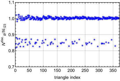
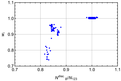
In order to estimate the accuracy of the integral approximation, we compare the continuous ($k_{f}\to 0$ limit) prediction for the number of triangle modes that fall in a given bin $N_{123}$ with the actual number of discrete triangles in that bin $N_{B}^{\rm disc.}$. The result is shown in the upper left panel of Fig. 1, where we display the ratio $N_{B}^{\rm disc.}/N_{123}$ for the bins whose centers satisfy the momentum conservation constraint, and which we actually use in the analysis. We see that the integral approximation correctly predicts the number of fundamental triangles for most of the bins, up to a few percent precision. However the integral approximation is not very accurate for folded triangles with $k_{2}+k_{3}=k_{1}+\Delta k/2$. For these triangles the typical mismatch is about $\sim 15\%$. This discrepancy also leads to a mismatch at the level of binned bispectra. To correct for this discrepancy we introduce “discreteness weights” $w$,

$$w=\frac{\hat{B}_{\rm disc}}{\hat{B}_{\rm int}}\,,$$ (3.27)

where $\hat{B}_{\rm disc}$ is computed by using a direct discrete expression Eq. (3.22), while $\hat{B}_{\rm int}$ is calculated from Eq. (3.25).

We compute the weights for a certain fiducial cosmology and nuisance parameters extracted from a fit to the simulation data analyzed without the weights. Since the evaluation of the full discrete expression Eq. (3.22) is too expensive for an Markov chain Monte Carlo (MCMC), the best strategy would be to iterate the discreetness weights for the best-fit bispectra from a few consecutive MCMC runs. However, quite remarkably, we have found that this iterative procedure has converged already at the first step. Our initial fiducial parameters happened to be significantly different from the actual best-fit parameters, yet both produced almost identical discreteness weights. This shows that the discreetness weights are nearly cosmology-independent, hence they can be computed only once for a given survey specification.

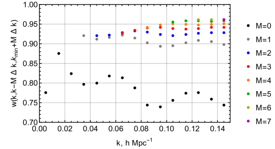
We display the discreteness weights for PT challenge boxes in the right panel of Fig. 1, along with the ratio $N_{B}^{\rm disc.}/N_{123}$, which demonstrates that the “problematic” triangles can be easily identified in the data by comparing the number of fundamental triangles in the bin with the prediction of the integral approximation. As we can see from this figure, these corrections need to be included if $N_{B}^{\rm disc.}/N_{123}$ deviates from unity by more than $10\%$. We show discreteness weights specifically for the problematic folded triangles in the lower panel of Fig. 1. For all other triangle configurations the discreteness weights coincide with unity with $\mathcal{O}(0.5)\%$ precision, implying that the integral approximation is very accurate for them.

Additionally, we validate our discreteness weights approach in Appendix A by comparing it with an approximate discrete binning scheme similar to Eq. (3.22). These tests suggest that our treatment of discreteness effects is accurate enough for the full simulation volume and hence can be safely adopted for the purposes of our paper and for any realistic future analysis.

All in all our theory model is given by

$$B^{\rm th}=\hat{B}^{\rm int}_{0}(k_{1},k_{2},k_{3})w(k_{1},k_{2},k_{3})\,,$$ (3.28)

where $\hat{B}^{\rm int}_{0}$ is computed from Eq. (3.26) by numerically performing the five-dimensional integral over the tree-level IR resummed model (3.14).

4 Likelihood

We will use a Gaussian likelihood for the bispectrum [3],

$$\mathop{\rm ln}\nolimits\mathcal{L}_{\rm B}=-\frac{1}{2}\sum_{\text{triangles}~{}T^{\prime}}(B^{\rm th}_{T}-B^{\rm data}_{T})(B^{\rm th}_{T^{\prime}}-B^{\rm data}_{T^{\prime}})(C^{\rm B})^{-1}_{TT^{\prime}}\,,$$ (4.1)

where we assume without loss of generality that the bin centers satisfy $k_{1}\geq k_{2}\geq k_{3}$ and

$$\begin{split}&\sum_{T}\equiv\sum_{k_{1}=k_{\rm min}}^{k_{\rm max}}\sum_{k_{2}=k_{\rm min}}^{k_{1}}\sum_{k_{3}=k_{*}}^{k_{2}}\,,\quad k_{*}\equiv\text{max}(k_{\rm min},k_{1}-k_{2})\,.\end{split}$$ (4.2)

The Gaussian likelihood approximation for the bispectrum is justified within perturbation theory, which is consistent with the tree-level approximation for the bispectrum itself. This approximation must be true on sufficiently large scales, to which we limit our analysis. In this regime we can use the Gaussian tree-level approximation for the covariance matrix $C^{\rm B}$ [38, 3, 94, 20],

$$\begin{split}&C^{\rm B}_{TT^{\prime}}=\frac{(2\pi)^{3}\pi s_{123}}{k_{1}k_{2}k_{3}\Delta k^{3}V_{\rm tot}}\delta_{TT^{\prime}}\int_{0}^{2\pi}\frac{d\phi}{4\pi}\int_{-1}^{1}d\mu~{}\prod_{i=1}^{3}\left[P_{\rm lin}(k_{i})(b_{1}+f\mu^{2}_{i}(\phi,\mu))^{2}+\frac{1}{\bar{n}}\right]\,,\end{split}$$ (4.3)

where $(k_{1},k_{2},k_{3})$ denotes the center of the triangle bin $T$, $V_{\rm tot}$ is the cumulative volume of the PT challenge simulations ($V_{\rm tot}=566~{}h^{-3}$Gpc³), $s_{123}=~{}$6, 2 or 1 for equilateral, isosceles and general triangles. To approximately account for the discreteness binning effects we use the true number of fundamental triangles in the bin instead of the prediction of the integral approximation, i.e. we rescale

$$C^{\rm B}_{TT^{\prime}}\to\frac{N_{123}}{N^{\rm disc}_{B}}\cdot C^{\rm B}_{TT^{\prime}}\,.$$ (4.4)

We evaluate the covariance for the best-fit cosmology extracted from the power spectrum likelihood analysis. We ignore the cross-covariance between the power spectrum and the bispectrum in our baseline analysis. This and other likelihood approximations are validated in Appendix C. There we show that our results are stable if we include the one-loop theoretical error bispectrum covariance, and the cross-covariance between the power spectrum and bispectrum (computed in perturbation theory), as well as if we replace the Gaussian bispectrum covariance with the sample covariance from the available mocks. All these different options yield statistically indistinguishable results.

Our total likelihood thus consists of a product of the bispectrum and baseline power spectrum likelihoods,

$$\mathcal{L}_{\rm tot}=\mathcal{L}_{\rm B}\times\mathcal{L}_{\rm P}\,.$$ (4.5)

The details of our baseline power spectrum likelihood can be found in Appendix D and in Ref. [73]. We compute power spectrum theoretical templates using the CLASS-PT code [41]. We run MCMC chains using the Montepython code [100, 101]. Posterior density plots are generated with the getdist package [102]. We will scan over the parameters of the base $\Lambda$CDM model and EFT nuisance parameters [51, 50],

$$\{\omega_{cdm},H_{0},A_{s},n_{s}\}\times\{b_{1},b_{2},b_{\mathcal{G}_{2}},b_{\Gamma_{3}},c_{0},c_{2},b_{4},a_{0},a_{2},P_{\rm shot},B_{\rm shot},c_{1}\}\,.$$ (4.6)

The priors on the power spectrum nuisance parameters are given in Appendix D. As for $B_{\rm shot}$, we place a Gaussian prior on it with unit mean, which corresponds to the Poissonian sampling prediction, and unit variance,

$$B_{\rm shot}\sim\mathcal{N}(1,1^{2})\,.$$ (4.7)

$c_{1}$ is varied in our MCMC chains without any priors, unless otherwise stated. We fix the physical baryon density to its true value in order to simulate the BBN prior as it was used in Refs. [45, 50].

5 Results

We start our analysis from the simple case of the real space bispectrum, which is free from RSD and projection effects. Then, we will analyze a setup that closely matches an actual spectroscopic survey: we will study the bispectrum in redshift space and in the presence of the projection effect. Since the PT challenge data which we are using is still ongoing, we report the measurements of all cosmological parameters normalized to their true injected values. As far as nonlinear bias parameters are concerned, we will present their values after the subtraction of the fiducial values extracted from our best-fit estimates from the most constraining baseline likelihood analysis. Specifically, we will report

$$\Delta b_{2}\equiv b_{2}-b^{\rm bf}_{2}\,,\quad\Delta b_{\mathcal{G}_{2}}\equiv b_{\mathcal{G}_{2}}-b^{\rm bf}_{\mathcal{G}_{2}}\,,\$$ (5.1)

where $b^{\rm bf}_{2},b^{\rm bf}_{\mathcal{G}_{2}}$ are best-fit values extracted from the fiducial analysis of the redshift space power spectrum combined with the real space bispectrum at $k_{\rm max}=0.08~{}h$/Mpc. This will be our best guess for the true values of these parameters.

We emphasize that expect for Section 5.4, in all our analysis the scale cuts of the power spectrum likelihood are kept fixed. Only $k_{\rm max}$ of the bispectrum data is varied.

Figure 2: Posterior distributions of cosmological and some nuisance parameters from MCMC analyses of the joint redshift-space power spectrum and real space bispectrum data. We show results for five different choices of the bispectrum data cut $k_{\rm max}$. All cosmological parameters and $b_{1}$ are normalized to their true values. We have subtracted constant fiducial values from the quadratic bias parameters $b_{2}$ and $b_{\mathcal{G}_{2}}$. Results for the power spectrum data only are shown for comparison.

Figure 3: Bispectrum data points from the PT challenge simulations along with best-fit theoretical predictions extracted from our MCMC chains. We show the bispectra for squeezed, equilateral and isosceles triangles (left panels), and the corresponding residuals (right panels).

Figure 4: Residuals between the bispectrum data and best-fitting theory templates for all triangles from the real space (left panel), and the redshift space (right panel) analyses.

5.1 Redshift space power spectrum + real space bispectrum

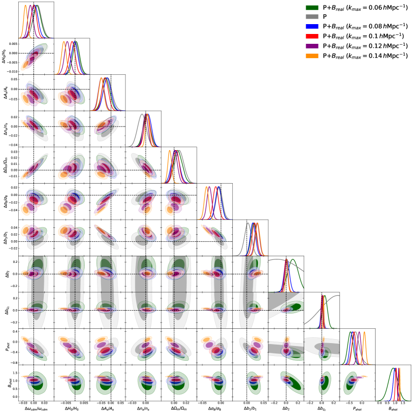
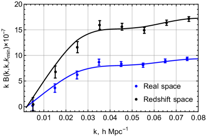
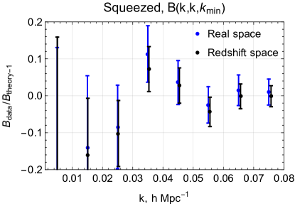
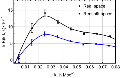
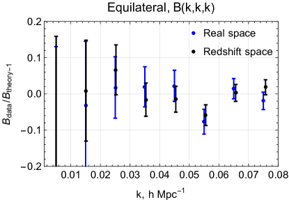
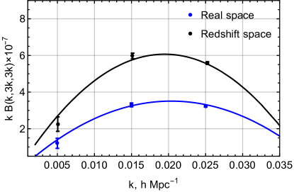
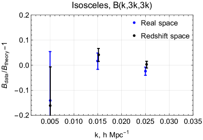
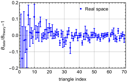
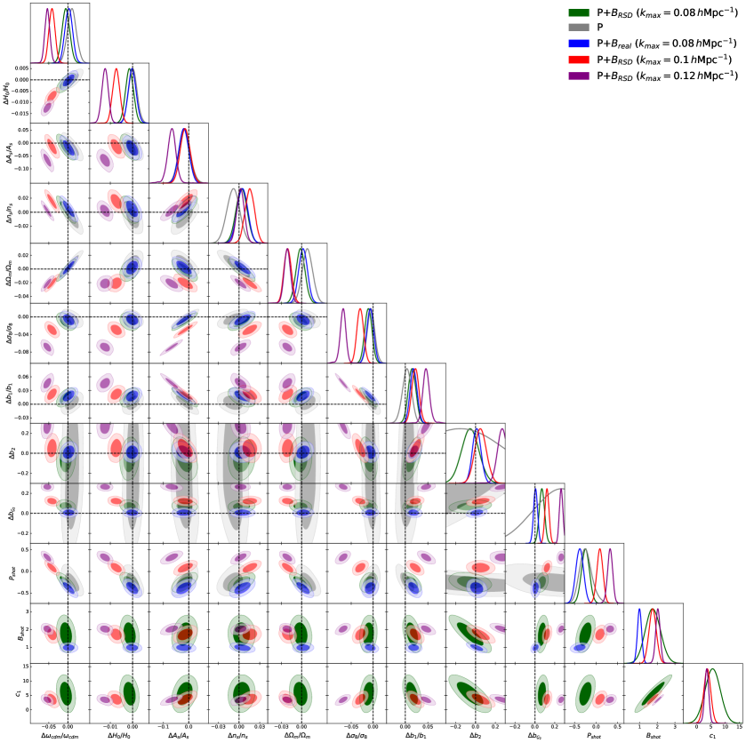
We start with the real space bispectrum, which can be formally obtained from our model Eq. (3.14) by setting $f=0,~{}c_{1}=0$, and ignoring the AP effect. We also note that the discreteness weights are closer to unity in this case. This can be attributed to the absence of leakage from higher angular moments [75], which is present in the redshift-space case. We perform our analysis for the bispectrum for five choices of $k_{\rm max}$ ranging from $0.06$ to $0.14~{}h\text{Mpc}^{-1}$ with a step $0.02~{}h\text{Mpc}^{-1}$. The resulting corner plot from our MCMC analyses is shown in Fig. 2, and the 1d marginalized limit for the case $k_{\rm max}=0.08h\text{Mpc}^{-1}$ are presented in Table 1. The best fitting curves for certain triangle configurations are shown in Fig. 3, while Fig. 4 is a residual plot over all triangles used in the fit.

Power
Parameter	68% limits
$\Delta H_{0}/H_{0}$	$0.0001\pm 0.0019$
$\Delta\omega_{cdm}/\omega_{cdm}$	$0.010\pm 0.012$
$\Delta A_{s}/A_{s}$	$-0.016\pm 0.022$
$\Delta n_{s}/n_{s}$	$-0.0084\pm 0.0094$
$\Delta b_{1}/b_{1}$	$0.003\pm 0.010$
$\Delta b_{2}$	$-0.13^{+0.44}_{-0.51}$
$\Delta b_{\mathcal{G}_{2}}$	$0.29\pm 0.30$
$P_{{shot}}$	$-0.24^{+0.12}_{-0.16}$
$\Delta\sigma_{8}/\sigma_{8}$	$-0.0045\pm 0.0087$
$\Delta\Omega_{m}/\Omega_{m}$	$0.0087\pm 0.0077$
$\frac{b_{1}^{3}\sigma_{8}^{4}}{(b_{1}^{3}\sigma_{8}^{4})_{\rm fid.}}-1$	$-0.008\pm 0.022$

Power+real space bispectrum
Parameter	68% limits
$\Delta H_{0}/H_{0}$	$-0.0002\pm 0.0018$
$\Delta\omega_{cdm}/\omega_{cdm}$	$0.0022\pm 0.0098$
$\Delta A_{s}/A_{s}$	$-0.019\pm 0.019$
$\Delta n_{s}/n_{s}$	$0.0048\pm 0.0076$
$\Delta b_{1}/b_{1}$	$0.0183\pm 0.0077$
$\Delta b_{2}$	$0.011\pm 0.043$
$\Delta b_{\mathcal{G}_{2}}$	$0.006\pm 0.020$
$P_{{shot}}$	$-0.384\pm 0.089$
$B_{{shot}}$	$0.99\pm 0.12$
$\Delta\sigma_{8}/\sigma_{8}$	$-0.0065\pm 0.0080$
$\Delta\Omega_{m}/\Omega_{m}$	$0.0022\pm 0.0064$
$\frac{b_{1}^{3}\sigma_{8}^{4}}{(b_{1}^{3}\sigma_{8}^{4})_{\rm fid.}}-1$	$0.028\pm 0.016$

RSD bispectrum
Parameter	68% limits
$\Delta H_{0}/H_{0}$	$-0.026\pm 0.015$
$\Delta\omega_{cdm}/\omega_{cdm}$	$-0.026\pm 0.032$
$\Delta A_{s}/A_{s}$	$-0.07^{+0.17}_{-0.35}$
$\Delta n_{s}/n_{s}$	$-0.018\pm 0.034$
$\Delta b_{1}/b_{1}$	$0.07^{+0.20}_{-0.26}$
$\Delta b_{2}$	$0.81^{+0.26}_{-0.33}$
$\Delta b_{\mathcal{G}_{2}}$	$0.270^{+0.068}_{-0.091}$
$c_{1}$	$-2.4\pm 3.8$
$P_{{shot}}$	$-0.095\pm 0.93$
$B_{{shot}}$	$0.89^{+0.69}_{-0.61}$
$\Delta\sigma_{8}/\sigma_{8}$	$-0.07^{+0.11}_{-0.16}$
$\Delta\Omega_{m}/\Omega_{m}$	$0.033^{+0.032}_{-0.039}$
$\frac{b_{1}^{3}\sigma_{8}^{4}}{(b_{1}^{3}\sigma_{8}^{4})_{\rm fid.}}-1$	$-0.194^{+0.082}_{-0.074}$

Power+RSD bispectrum
Parameter	68% limits
$\Delta H_{0}/H_{0}$	$-0.0014\pm 0.0018$
$\Delta\omega_{cdm}/\omega_{cdm}$	$-0.005\pm 0.010$
$\Delta A_{s}/A_{s}$	$-0.017\pm 0.021$
$\Delta n_{s}/n_{s}$	$0.0036\pm 0.0080$
$\Delta b_{1}/b_{1}$	$0.0149\pm 0.0085$
$\Delta b_{2}$	$-0.054\pm 0.088$
$\Delta b_{\mathcal{G}_{2}}$	$0.070\pm 0.026$
$c_{1}$	$5.6\pm 2.7$
$P_{{shot}}$	$-0.249\pm 0.093$
$B_{{shot}}$	$1.75\pm 0.43$
$\Delta\sigma_{8}/\sigma_{8}$	$-0.0107\pm 0.0082$
$\Delta\Omega_{m}/\Omega_{m}$	$-0.0017\pm 0.0068$
$\frac{b_{1}^{3}\sigma_{8}^{4}}{(b_{1}^{3}\sigma_{8}^{4})_{\rm fid.}}-1$	$0.001\pm 0.016$

Table 1: 1d marginalized limit for the cosmological and most important nuisance parameters from various PT challenge likelihoods: redshift space power spectrum only (upper left panel), the joint power spectrum + real space bispectrum (upper right panel), redshift space bispectrum only (lower left panel), and the joint redshift space power spectrum + redshift space bispectrum (lower right panel). Parameters that were directly varied in MCMC chains are displayed in the upper part of the table, the lower groups contain derived parameters. Most parameters are normalized to their true values. See the main text for more detail.

We observe that inclusion of the bispectrum sharpens estimates for all cosmological and bias parameters and does not lead to any significant biases up to $k_{\rm max}=0.08h\text{Mpc}^{-1}$. We see some small biases, especially in the $b_{1}-\sigma_{8}$ plane, but our MCMC posteriors still enclose the true values within $99\%$ CL, which makes these shifts compatible with statistical fluctuations. Besides, these small shifts do not change when switching the bispectrum data cut from $0.06h\text{Mpc}^{-1}$ to $0.08h\text{Mpc}^{-1}$. In contrast, for $k_{\rm max}>0.08h\text{Mpc}^{-1}$ we see clear shifts that push estimated values away from the ground truth. In particular, we find the bias on $\sigma_{8}$ to be $[-1.9,-5.2,-6.7]\sigma$ for $k_{\rm max}/h\text{Mpc}^{-1}=[0.1,0.12,0.14]$, respectively. This suggests us to adopt $k_{\rm max}=0.08h\text{Mpc}^{-1}$ as a baseline data cut for the real space bispectrum in what follows.

The tree-level bispectrum likelihood improves constraints on cosmological and some nuisance parameters. This improvement can be estimated by ratios of the 1d marginalized $68\%$ confidence intervals. For the cosmological parameters we have

$$\frac{\sigma_{\rm P+B}}{\sigma_{\rm P}}\{\omega_{cdm},h,n_{s},A_{s},\Omega_{m},\sigma_{8}\}=\{0.82,0.90,0.81,0.88,0.83,0.93\}\,$$

indicating a $(10-20)\%$ improvement in most cases. The gain is more sizable for the nuisance parameters,

$$\frac{\sigma_{\rm P+B}}{\sigma_{\rm P}}\{b_{1},b_{2},b_{\mathcal{G}_{2}},P_{\rm shot}\}=\{0.75,0.09,0.07,0.61\}\,.$$

Intuitively, this happens because in the bispectrum one can probe the galaxy bias parameters from large scales, and hence their determination is not contaminated by loop corrections and additional nuisance parameter marginalization.

The picture that we have observed here is in stark contrast with the real space only results, presented in Appendix E. This analysis shows that the real space power spectrum has much less information than the redshift-space one. In this case the combination with the bispectrum leads to a dramatic shrinking of posterior distributions for both cosmological and nuisance parameters. However, in redshift space the power spectrum has much more information to begin with, and thus the addition of the bispectrum yields only a moderate improvement.

5.2 Bias parameters

Our simulated galaxies are produced with simple HOD models and therefore one may expect their nonlinear bias parameters to match those of the host halos and to follow the same dependence on $b_{1}$. Let us compare this expectations with reality. For the tidal bias $b_{\mathcal{G}_{2}}$, as a first guess, we can use the so-called Lagrangian Local In Matter Density (LLIMD) bias model prediction $b_{\mathcal{G}_{2}}^{\rm LLIMD}=-2(b_{1}-1)/7$ [67]. Using the fiducial value of $b_{1}$ we find

$$\Delta b_{\mathcal{G}_{2}}^{\rm LLIMD}=-\frac{2}{7}(b^{\rm fid}_{1}-1)-b_{\mathcal{G}_{2}}^{\rm fid}=0.23\,,$$ (5.2)

which is more that $10\sigma$ away from the truth. The LLIMD approximation is known to be in tension with high precision simulation measurements, which clearly show the evidence for the tidal Lagrangian bias [105]. A better fit to this data is a coevolution model with the initial Lagrangian bias that has the following dependence on the mean halo mass $M$

$$b^{L}_{\mathcal{G}_{2}}=-0.5\left(\frac{M}{4\times 10^{14}h^{-1}M_{\odot}}\right)^{0.8}\,.$$ (5.3)

Ref. [105] also presents the function $M(b_{1})$, from which we can express the above equation as $b^{L}_{\mathcal{G}_{2}}(b_{1})$. Inserting there our measurement of $b_{1}$, we find

$$\Delta b_{\mathcal{G}_{2}}^{\rm LTCM}=-\frac{2}{7}(b^{\rm fid}_{1}-1)+b^{L}_{\mathcal{G}_{2}}(b^{\rm fid}_{1})-b_{\mathcal{G}_{2}}^{\rm fid}=0.072\,,$$ (5.4)

where ‘LTCM’ stands for ‘Lagrangian tidal coevolution model’. We see that our measurement is still in $\sim 3\sigma$ tension with the prediction of LTCM, although in absolute terms the discrepancy is quite small. The discrepancy with the excursion set prediction from Ref. [106] is also quite high, it exceeds 10$\sigma$ in terms of the standard deviation of our measurement.

As far as $b_{2}$ is concerned, we can compare our measurement with the fit to halos from Refs. [107, 108], i.e. to consider

$$\Delta b_{2}^{\rm halo}=b^{\rm halo}_{2}(b^{\rm fid}_{1},b^{\rm fid}_{\mathcal{G}_{2}})-b_{2}^{\rm fid}=-0.49\,,$$ (5.5)

where

$$b^{\rm halo}_{2}(b_{1},b_{\mathcal{G}_{2}})=0.412-2.143b_{1}+0.929b_{1}^{2}+0.008b_{1}^{3}+\frac{4}{3}b_{\mathcal{G}_{2}}\,.$$ (5.6)

Note that we have accounted for the difference in our definition of quadratic biases w.r.t. Refs. [107, 108],

$$b^{\rm this\,work}_{\mathcal{G}_{2}}=b^{\rm previous}_{\mathcal{G}_{2}}\,,\quad b_{2}^{\rm this\,work}=b_{2}^{\rm previous}+\frac{4}{3}b^{\rm this\,work}_{\mathcal{G}_{2}}\,.$$ (5.7)

Thus, our analysis confirms significant deviations between the bias coefficients of galaxies and halos, which have already been pointed out in the literature [98, 109]. We also confirm the trend seen in the literature for the CMASS-like galaxies [44](similar to our PT challenge sample): the tidal bias of galaxies is lower than that of halos, but $b_{2}$ is higher. In particular, the results of Ref. [98] for the CMASS galaxies read

$$b_{2}^{\rm gal}=-0.2\pm 0.1\,,\quad b^{\rm gal}_{\mathcal{G}_{2}}=-0.46\pm 0.06\,.$$ (5.8)

These values can be compared with the predictions of the local Lagrangian approximation and the fit to $b_{2}$,

$$\begin{split}\text{Ref.~{}\cite[cite]{[\@@bibref{Number}{Eggemeier:2021cam}{}{}]}:}\quad&\Delta b_{2}=b^{\rm halo}_{2}(b^{\rm gal}_{2},b^{\rm gal}_{\mathcal{G}_{2}})-b^{\rm gal}_{2}=-0.41\pm 0.1\,,\\ &\Delta b_{\mathcal{G}_{2}}=b^{\rm LLIMD}_{\mathcal{G}_{2}}-b^{\rm gal}_{\mathcal{G}_{2}}=0.17\pm 0.06\,.\end{split}$$ (5.9)

These estimates perfectly agree with our results

$$\Delta b_{2}=-0.49\pm 0.04\,,\quad\Delta b_{\mathcal{G}_{2}}=0.23\pm 0.02\,.$$ (5.10)

Finally, let us discuss the cubic tidal bias parameter $b_{\Gamma_{3}}$. At the power spectrum level it is almost fully degenerate with $b_{\mathcal{G}_{2}}$. However, this degeneracy gets broken by the bispectrum data, since only $b_{\mathcal{G}_{2}}$ enters the tree-level bispectrum model. We will compare our measurements with halo relations obtained in Refs. [105, 106],

$$\begin{split}\text{Ref.~{}\cite[cite]{[\@@bibref{Number}{Abidi:2018eyd}{}{}]}:}\quad&b_{\Gamma_{3}}^{\rm halo}=-b_{\mathcal{G}_{2}}-\frac{1}{15}(b_{1}-1)\,,\\ \text{Ref.~{}\cite[cite]{[\@@bibref{Number}{Eggemeier:2020umu}{}{}]}:}\quad&b_{\Gamma_{3}}^{\rm halo}=-\frac{1}{6}(b_{1}-1)-\frac{3}{2}b_{\mathcal{G}_{2}}\,.\end{split}$$ (5.11)

This gives us a tension between our results and these halo predictions at the 2$\sigma$ level,

$$\begin{split}\text{Ref.~{}\cite[cite]{[\@@bibref{Number}{Abidi:2018eyd}{}{}]}:}\quad&b_{\Gamma_{3}}^{\rm gal}-b_{\Gamma_{3}}^{\rm halo}(b_{1}^{\rm gal},b_{\mathcal{G}_{2}}^{\rm gal})=0.23\pm 0.11\,,\\ \text{Ref.~{}\cite[cite]{[\@@bibref{Number}{Eggemeier:2020umu}{}{}]}:}\quad&b_{\Gamma_{3}}^{\rm gal}-b_{\Gamma_{3}}^{\rm halo}(b_{1}^{\rm gal},b_{\mathcal{G}_{2}}^{\rm gal})=0.24\pm 0.11\,.\end{split}$$ (5.12)

However, here we see the difference w.r.t. the CMASS-like sample of Ref. [98] ($b_{\Gamma_{3}}=-7\gamma_{21}/4$ in their notation). The relevant measurement from this work is fully consistent with that of halos,

$$b^{\rm CMASS}_{\Gamma_{3}}-b_{\Gamma_{3}}^{\rm halo}(b_{1}^{\rm gal},b_{\mathcal{G}_{2}}^{\rm gal})=-0.02\pm 0.14\,.$$ (5.13)

The discrepancy between our $b_{\Gamma_{3}}$ and that of Ref. [98] is marginally below $2\sigma$, and hence our measurements can be considered consistent.

Overall, we conclude that with the PT challenge simulations we see a $\sim 3\sigma$ discrepancy between the bias parameters of our HOD galaxies and their host halos. On the one hand, our bias parameter measurements agree well with those from similar mock CMASS-like galaxies, analyzed in Ref. [98].

Figure 5: Posterior distributions of cosmological and certain nuisance parameters from MCMC analyses of the joint redshift space power spectrum and redshift space bispectrum monopole data. We show results for three different choices of the bispectrum data cut $k_{\rm max}$. All cosmological parameters and $b_{1}$ are normalized to their true values. We have subtracted constant fiducial values from the quadratic bias parameters $b_{2}$ and $b_{\mathcal{G}_{2}}$. Results for the power spectrum (“$P$”) and for the power spectrum+real space bispectrum (“$P+B_{\rm real}~{}(k_{\rm max}=0.08~{}h\text{Mpc}^{-1})$”) datasets are shown for comparison.

Figure 6: Posterior distributions of cosmological and certain nuisance parameters from MCMC analyses of the redshift space power spectrum, redshift space bispectrum and their combination. We use $k_{\rm max}=0.08~{}h\text{Mpc}^{-1}$ for the bispectrum here.

5.3 Redshift space

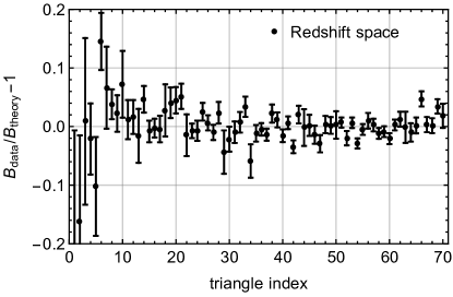
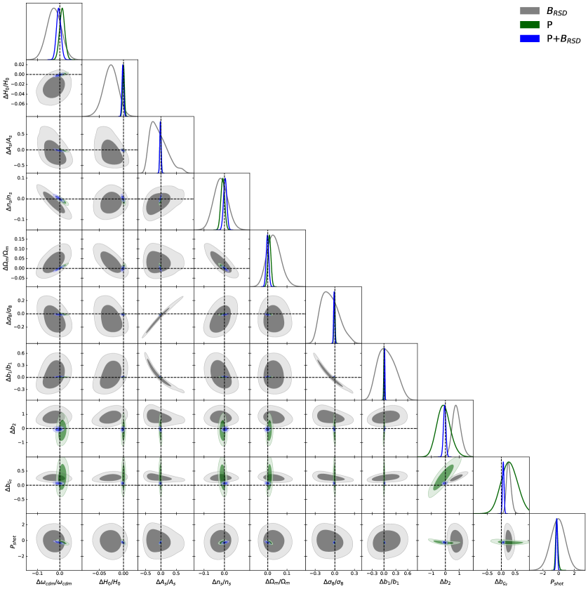
We now consider the realistic case of the redshift-space bispectrum monopole in the presence of the AP effect. We analyze our joint power spectrum and bispectrum likelihoods for three choices of the bispectrum data cut ranging $k_{\rm max}$ from $0.08~{}h\text{Mpc}^{-1}$ to $0.12~{}h\text{Mpc}^{-1}$ with a step $0.02~{}h\text{Mpc}^{-1}$. Our triangle plot is displayed in Fig. 5, where for comparison we also show the results of the baseline real space bispectrum analysis from the previous section. Marginalized 1d limits are presented in Table 1. Best-fit curves and the residual plot are shown in Fig. 3 and in Fig. 4.

We see that at $k_{\rm max}=0.08~{}h\text{Mpc}^{-1}$ the addition of the bispectrum likelihood slightly narrows the power spectrum contours and does not lead to any significant bias. Both cosmological and nuisance parameters are recovered within $95\%$ confidence intervals. However, already at $k_{\rm max}=0.08~{}h\text{Mpc}^{-1}$ we observe some evidence for the non-zero FoG counterterm $c_{1}$, which suggests that the one-loop corrections may not be negligible. Indeed, for more aggressive data cuts $k_{\rm max}>0.08~{}h\text{Mpc}^{-1}$ we find large biases that signal the breakdown of the tree-level bispectrum model. These biases are more significant than those that we have seen in the real space power spectrum likelihood, which is an expected consequence of non-linear redshift space distortions [38, 110, 61, 51, 111, 43]. A similar conclusion that FoGs in the bispectrum are important even on relatively large scales was made in Ref. [112]. These results motivate us to choose $k_{\rm max}=0.08~{}h\text{Mpc}^{-1}$ as our baseline data cut.

In Fig. 6 and table 1 we display the breakdown of different likelihoods in terms of their parameter constraints, including the redshift space bispectrum alone. Clearly, the constraints on cosmological parameters are heavily dominated by the power spectrum data. In part, this is a result of using only relatively low wavenumbers in our bispectrum analysis.

The bispectrum likelihood adds new information mostly through the bias parameter measurements. In particular, the principle component of the $b_{1}-\sigma_{8}$ degeneracy can be well approximated by a combination $b_{1}^{3}\sigma_{8}^{4}$, which captures the galaxy bispectrum amplitude in the absence of quadratic biases and projection effects. Our redshift space bispectrum-only analysis yields a measurement quite competitive with the redshift-space power spectrum result, c.f. table 1. Beside $b_{1}-\sigma_{8}$, the bispectrum also adds significant information through the quadratic bias parameters $b_{2}$ and $b_{\mathcal{G}_{2}}$, whose measurements from the bispectrum alone are more precise than from the power spectrum.

Addition of the bispectrum leads to following improvements on cosmological and nuisance parameters

$$\begin{split}&\frac{\sigma_{\rm P+B}}{\sigma_{\rm P}}\{\omega_{cdm},h,n_{s},A_{s},\Omega_{m},\sigma_{8}\}=\{0.88,0.94,0.86,0.95,0.89,0.96\}\,,\\ &\frac{\sigma_{\rm P+B}}{\sigma_{\rm P}}\{b_{1},b_{2},b_{\mathcal{G}_{2}},P_{\rm shot}\}=\{0.84,0.18,0.09,0.65\}\,.\end{split}$$ (5.14)

In general, the gain here is more modest compared to what we have obtained from the real space bispectrum. One reason for that is the correlation between the additional FoG counterterm $c_{1}$ and other parameters. For example, the degeneracy between $c_{1}$ and $b_{2},B_{\rm shot}$ is quite significant, which explains why the confidence intervals for these nuisance parameters are noticeably larger than those of the real space bispectrum case. Another reason for the relatively small improvement in cosmological parameters is that the BAO wiggles are more suppressed in redshift space, c.f. Eq. (3.12), and hence there is less available distance information.

All in all, the upshot of our analysis is that for the full PT challenge simulation volume the data cut for the tree-level redshift-space bispectrum model is $k_{\rm max}=0.08~{}h\text{Mpc}^{-1}$, and the addition of the bispectrum likelihood yields $\lesssim 10\%$ improvement on cosmological parameters, but much larger gains on bias parameters.

Figure 7: Same as Fig. 5 but with the covariance rescaled by $100$ to match the BOSS survey volume.

5.4 Forecast for BOSS

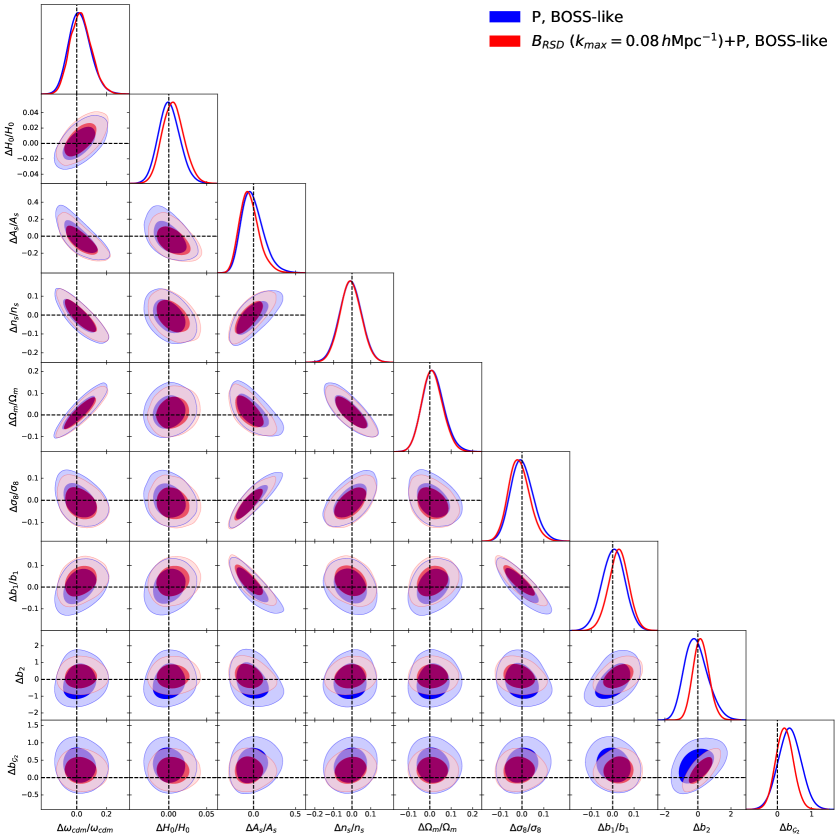
It is useful to re-run our analysis for the covariance that matches the volume of the currently available BOSS data. In this case the covariance is larger, and hence we can use more aggressive data cuts provided that the bias in cosmological parameters due to higher order loop corrections is smaller than a fraction of the statistical error. In this case the power spectrum multipole analysis can be pushed to $k_{\rm max}=0.20~{}h\text{Mpc}^{-1}$, which is noticeably larger than our baseline PT challenge power spectrum multipole data cut $k_{\rm max}=0.14~{}h\text{Mpc}^{-1}$ [50]. Note that this $k_{\rm max}$ is lower than $k_{\rm max}=0.25~{}h\text{Mpc}^{-1}$ used in Refs. [45, 113] because here we include the hexadecapole moment, see Ref. [50] for more detail. Consequently, the transverse power spectrum moment $Q_{0}$ is taken in the range $0.2<k/(h\text{Mpc}^{-1})<0.4$ [73]. Unfortunately, we cannot push the bispectrum analysis to $k_{\rm max}=0.1~{}h\text{Mpc}^{-1}$ because the relative theory systematic error on $\sigma_{8}$ there is around $3\%$. This is a significant fraction of the BOSS statistical error, $\sigma_{\sigma_{8}}/\sigma_{8}\approx 5\%$. We have explicitly checked that the recovered value of $\sigma_{8}$ is biased by $1\sigma$ of the BOSS error when the bispectrum is taken at $k_{\rm max}=0.1~{}h\text{Mpc}^{-1}$. Therefore, we proceed with the same baseline cut as in the PT challenge analysis of the previous section, $k_{\rm max}=0.08~{}h\text{Mpc}^{-1}$.

We analyze the same PT challenge data but with the covariance rescaled by a factor $100$, which is the difference between the PT challenge volume and the BOSS survey volume $V_{\rm BOSS}\simeq 6$ $h^{-3}$Gpc³. In this particular analysis, we also impose the following Gaussian prior on $c_{1}$,

$$c_{1}\sim\mathcal{N}(0,5^{2})\,,$$ (5.15)

which is motivated by the EFT expectation $c_{1}=\mathcal{O}(1)$. Our results are shown in Fig. 7 and in Table 2.

We observe that the addition of the bispectrum has roughly the same impact for cosmological parameters are the full PT challenge case, i.e. there is a $\sim 10\%$ improvement on the 1d marginalized constraint on $A_{s}$ and $\sigma_{8}$, and barely any effect on other parameters. As far as quadratic bias parameters are concerned, the improvements for them are less sizable. In contrast to the full PT challenge simulation, in the BOSS-like power spectrum case the bias parameters are dominated by priors (given in Appendix D) and not by the data. Hence, the power spectrum posteriors are narrower to begin with. Still, the addition of the bispectrum data sharpens $b_{2}$ and $b_{\mathcal{G}_{2}}$ posteriors by a factor of two.

Power spectrum (PS), BOSS-like
Parameter	68% limits
$\Delta H_{0}/H_{0}$	$0.001^{+0.013}_{-0.015}$
$\Delta\omega_{cdm}/\omega_{cdm}$	$0.021^{+0.065}_{-0.080}$
$\Delta A_{s}/A_{s}$	$-0.01^{+0.10}_{-0.15}$
$\Delta n_{s}/n_{s}$	$-0.009\pm 0.059$
$\Delta b_{1}/b_{1}$	$0.004\pm 0.053$
$\Delta b_{2}$	$-0.09^{+0.59}_{-0.80}$
$\Delta b_{\mathcal{G}_{2}}$	$0.36\pm 0.33$
$P_{{shot}}$	$-0.13\pm 0.51$
$\Delta\sigma_{8}/\sigma_{8}$	$0.000^{+0.046}_{-0.055}$
$\Delta\Omega_{m}/\Omega_{m}$	$0.016^{+0.046}_{-0.055}$

PS + bispectrum, BOSS-like
Parameter	68% limits
$\Delta H_{0}/H_{0}$	$0.006^{+0.013}_{-0.015}$
$\Delta\omega_{cdm}/\omega_{cdm}$	$0.029^{+0.063}_{-0.080}$
$\Delta A_{s}/A_{s}$	$-0.049^{+0.093}_{-0.13}$
$\Delta n_{s}/n_{s}$	$-0.008\pm 0.057$
$\Delta b_{1}/b_{1}$	$0.028\pm 0.047$
$\Delta b_{2}$	$0.19^{+0.44}_{-0.50}$
$\Delta b_{\mathcal{G}_{2}}$	$0.21\pm 0.25$
$P_{{shot}}$	$-0.38\pm 0.40$
$B_{{shot}}$	$1.23\pm 0.89$
$c_{1}$	$0.1\pm 4.8$
$\Delta\sigma_{8}/\sigma_{8}$	$-0.013^{+0.044}_{-0.052}$
$\Delta\Omega_{m}/\Omega_{m}$	$0.012^{+0.045}_{-0.052}$

Table 2: 1d marginalized limits from analyses of the redshift space galaxy power spectrum (left panel) and the joint power and bispectrum data (right panel) from the PT challenge simulation with the covariance rescaled to match the volume of the BOSS survey, as shown in Fig. 7.

6 Comparison with Previous Work

Our analysis complements and extends other works on the galaxy bispectrum. Therefore, it is useful to compare our study with the most relevant literature.

Ref. [96] studied the real space halo galaxy bispectrum from simulations with the overall volume similar to that of the PT challenge suite. This work used the tree-level bispectrum model to fit the pure bispectrum data (in the absence of the power spectrum), and has established that this model works up to $k_{\rm max}=0.082~{}h\text{Mpc}^{-1}$, in agreement with our baseline result $k_{\rm max}=0.08~{}h\text{Mpc}^{-1}$. This work did not find any significant deviations from Poissonian sampling for the halo bispectrum. In contrast, we did find the sub-Poissonian shot noise for the PT challenge galaxies. Importantly, this detection is driven by the power spectrum data, which yields a $\gtrsim 2\sigma$ deviation from the Poissonian sampling even in the absence of any bispectrum data. This can be compared with the bispectrum data alone (see Fig. 6), which is not precise enough to constrain the shot noise. When the two likelihood are combined, we obtain much tighter constraints on the shot noise parameters than the bispectrum alone, which explains why our analysis is more sensitive to shot noise corrections than that of Ref. [96]. Nevertheless, our result is not surprising, given that on general grounds we do expect halo stochasticity to be different from that of galaxies, see e.g. [111]. The importance of beyond-Poissonian sampling for primordial non-Gaussianity constraints from the bispectrum was also emphasized in [10].

Ref. [98] presented constraints on the galaxy bias parameters from the combination of the real space power spectrum and bispectrum data. This work used a one-loop theoretical error model for the bispectrum, which allowed one to push the analysis to small scales and achieve parameter measurement precision similar to ours while using smaller effective volume $V_{\rm eff}=6~{}h^{-3}$ Gpc³. An important observation is our analysis confirms the result of Ref. [98] that the quadratic bias parameters of BOSS-like galaxies do not follow halo-calibrated dependencies on linear bias $b_{1}$. The deviations from these dependencies that we find in our work agree very well with those reported in Ref. [98].

It is also worth comparing conclusions on the cosmological parameter improvements from the bispectrum in real space from Ref. [98] and from our redshift space analysis. Ref. [98] showed that constraints on $A_{s}$ typically improve by factors of $4-6$ in real space. This improvement factor stays roughly the same regardless of whether the tree-level or the one-loop bispectrum model is used. In contrast to this, our analysis implies that the bispectrum monopole sharpens the $A_{s}$ constraints only by $\sim 20\%$ in redshift space. This happens because the notorious degeneracy between the linear bias $b_{1}$ and $A_{s}$, which plagues real space analyses, is lifted in redshift space already at the level of power spectrum multipoles.

The bispectrum monopole of BOSS-like mocks and the actual bispectrum data from the CMASS north galactic cap (NGC) sample were analyzed in Ref. [46]. This analysis is closest to ours since it uses essentially a similar EFT theoretical model for the power spectrum part. However, its bispectrum analysis is different from ours by a number of instances. First, systematic errors in the window function treatment forced Ref. [46] to discard low wavenumber modes, i.e. use $k_{\rm min}=0.04~{}h\text{Mpc}^{-1}$. Second, similarly to us, the authors of Ref. [46] used the tree-level EFT model for the bispectrum monopole. However, they ignored IR resummation (which is necessary already at the tree level [69, 4]) and additional corrections due to FoG and binning, which was partly justified by the smallness of the total simulation volume of that work compared to ours. Nevertheless, the final scale cuts $k_{\rm max}=(0.08-0.1)~{}h\text{Mpc}^{-1}$ of the bispectrum analysis of Ref. [46] are consistent with our choice $k_{\rm max}=0.08~{}h\text{Mpc}^{-1}$. Finally, Ref. [46] found that the bispectrum data from one BOSS data chunk (CMASS NGC) sharpens the constrain on $A_{s}$ by $\lesssim 20\%$ and leaves intact other cosmological parameters. We have found a quantitatively similar behavior in our analysis, see Fig. 7. It will be interesting to see how much the constraints improve in the analysis of the actual BOSS data with our likelihood. We leave this for future work [116].

Finally, it is worth comparing our results with those from the MCMC forecast for the Euclid-like survey from Ref. [6]. This work used a very similar methodology and found that the addition of the tree-level bispectrum monopole likelihood leads to $\sim(10-50)\%$ on all relevant cosmological parameters of the $\Lambda$CDM model with massive neutrinos. Our analysis is different from Ref. [6] in several aspects. First, unlike Ref. [6], our baseline power spectrum likelihood contains the real space power spectrum $Q_{0}$ [73]. Moreover, our likelihood here includes physical priors on nuisance parameters, whereas Ref. [6] did not assume any priors on them. These two factors may diminish relative information content of the bispectrum in our work. Second, we analyze only one redshift bin here, whereas Ref. [6] considers a more realistic data sample spread across 8 different bins. Clearly, this latter case contains more distance information that can be extracted through the AP effect. Third, we impose the BBN prior on $\Omega_{b}$ here, while Ref. [6] fits this parameter directly from the large-scale structure data. Despite these significant differences, one observes a qualitative agreement between our results: in both cases the tree-level bispectrum monopole improves cosmological parameter constrains by tens of percent.

7 Conclusions

In this work we have studied the cosmological information present in the redshift-space bispectrum monopole of PT challenge simulation galaxies. We analyze the joint power spectrum and bispectrum likelihood using the one-loop EFT model for the power spectrum and the tree-level model for the bispectrum. This is a fully consistent approach as for both statistics we use the perturbative density field expanded to third order in the linear solution. Our bispectrum theoretical templates include, for the first time, all the effects that are needed to describe the data at this order: tree-level IR resummation, corrections due to discreteness, FoG, and the AP effect. Our main results are

• The tree-level bispectrum model is valid up to $k_{\rm max}=0.08~{}h\text{Mpc}^{-1}$ for a BOSS-like luminous red galaxy sample.

• The addition of the tree-level bispectrum likelihood to the power spectrum one leads to moderate improvements of constraints on cosmological parameters by $\lesssim 10\%$.

• The improvement on bias parameters is very significant. The errorbars on the quadratic local in density bias $b_{2}$ and the tidal bias $b_{\mathcal{G}_{2}}$ shrink by more than a factor of 10 after adding the bispectrum data.

• We have found that the quadratic galaxy bias parameters are quite different from biases of host dark matter halos. This confirms the trend seen in the literature [98, 109].

On the technical side, we have proposed a new efficient approach to account for binning effects by a combination of the integral approximation and discreteness weights, and also studied in detail the dependence of our results on bispectrum covariance matrix choices.

There are several ways to extend our analysis. First, it would be important to upgrade our theory model with the redshift-space one-loop bispectrum calculations. In particular, we have found that at $k_{\rm max}>0.08~{}h\text{Mpc}^{-1}$ the data shows evidence for FoG, which is a loop effect in the EFT nomenclature. Given that the one-loop calculation significantly extends the regime of validity of the EFT in the power spectrum case, one may expect that a similar improvement can take place for the bispectrum. It is important to notice that for consistency one needs to compute the power spectrum at two loop order when considering the one-loop bispectrum.

Moreover, it is also interesting to consider higher angular moments of the redshift-space bispectrum. Various forecasts suggest that these moments may contain significant cosmological information, see e.g. [5]. We plan to verify these results in an actual analysis of simulated or real data. Importantly, higher order bispectrum multipoles are sensitive to FoG, and hence one-loop corrections are desirable for their systematic study. This issue can be mitigated with an analog of the transverse moment $Q_{0}$ for the bispectrum. We plan to study this statistics in future.

Another natural step is the analysis of the actual bispectum data from the BOSS survey [116]. Our work suggests that the inclusion of the bispectrum may improve constraints on the mass fluctuation amplitude by $\sim 10\%$. This improvement is not very dramatic, but it should be pointed out that so far we have considered only the minimal $\Lambda$CDM model. The information content of the redshift space bispectrum can be richer in nonminimal cosmological models, which may have some implications for certain tensions, e.g. the so-called $\sigma_{8}$ tension [117].

Finally, it would be interesting to repeat our analysis for the emission line galaxies, which will be the main targets of future surveys like DESI [118] and Euclid [119, 120]. Emission line galaxies are less biased than the red luminous galaxies whose mocks we studied in this paper. Moreover, recent measurements suggest that they are less affected by FoG [121, 86], which implies that the EFT model may perform better for this sample.

Note added.

While this paper was being prepared, a new work [122] studying the information content of the real space bispectrum appeared. When results overlap, they are in agreement.

Acknowledgments.

We thank Giovanni Cabass, Roman Scoccimarro and Jay Wadekar for fruitful discussions. The work of MMI has been supported by NASA through the NASA Hubble Fellowship grant #HST-HF2-51483.001-A awarded by the Space Telescope Science Institute, which is operated by the Association of Universities for Research in Astronomy, Incorporated, under NASA contract NAS5-26555. OHEP thanks the Simons Foundation for support. This work was supported in part by MEXT/JSPS KAKENHI Grant Number JP19H00677, JP20H05861 and JP21H01081. We also acknowledge financial support from Japan Science and Technology Agency (JST) AIP Acceleration Research Grant Number JP20317829. The simulation data analysis was performed partly on Cray XC50 at Center for Computational Astrophysics, National Astronomical Observatory of Japan.

Appendix A Tests of Binning

In order to account for binning effects, one should ideally evaluate the full sum over all possible triangle configurations inside the bin. However, this evaluation is computationally very expensive. In the main text we have used the integral approximation along with discreteness weights that correct for the inaccuracy of this approximation for the folded triangles. In this appendix we present an alternative to this scheme, which works well for the real space bispectrum.

The main goal of our binning scheme is to generate many “fundamental” triangle configurations based on the true $k_{f}$ and then sum them into appropriate bins. It is computationally expensive to generate all the fundamental triangles on the actual 3d Fourier grid. Moreover, it is also not efficient, because the fundamental grid contains a large number of identical fundamental triangles. We can avoid that by organizing a sum over unique fundamental triangle configurations with $q_{1}\geq q_{2}\geq q_{3}$, where $q_{i}$ are wavevector moduli of fundamental triangles. In this case we need to sample the bispectra over a relatively small grid of wavenumbers. We will call this method “approximate 1d binning” in what follows. It is based, essentially, on taking the integral expression Eq. (3.26) and approximating it with a sum over appropriate discrete configurations of wavevector moduli.

Let us start with the integral approximation Eq. (3.26), obtained after eliminating most of angular variables by means of the Dirac delta-function. In real space the integrals over $\mu$ and $\phi$ drop out of this expression because the bispectrum does not depend on angles. Now we can write down the following discrete approximation to the final integral,

$$\begin{split}\hat{B}^{\rm int}_{0}\simeq\frac{V\sum_{123}q_{1}q_{2}q_{3}B(q_{1},q_{2},q_{3})}{V\sum_{123}q_{1}q_{2}q_{3}~{}1}\,,\end{split}$$ (A.1)

where the sum $\sum_{123}$ is taken over all configurations of momentum moduli $q_{i}$ that fall in the bin. This sum contains many indistinguishable modes. Now we replace this sum with a discrete sum over independent triangle configurations only,

$$\begin{split}\hat{B}^{\rm int}_{0}\simeq\frac{V\sum_{T}q_{1}q_{2}q_{3}B(q_{1},q_{2},q_{3})}{V\sum_{T}q_{1}q_{2}q_{3}~{}1}\,,\end{split}$$ (A.2)

where the sum $\sum_{T}$ runs over all unique triangles that fall in the bin $(k_{1},k_{2},k_{3})$ and that respect the $k_{f}$ spacing,

$$\sum_{T}\equiv\sum_{q_{1}=\text{max}(k_{f},k_{1}-\Delta k/2)}^{k_{1}+\Delta k/2}\sum_{q_{2}=\text{max}(k_{f},k_{2}-\Delta k/2)}^{\text{min}(k_{2}+\Delta k/2,q_{1})}\sum_{q_{3}=\text{max}(k_{f},k_{3}-\Delta k/2,q_{1}-q_{2})}^{\text{min}(k_{3}+\Delta k/2,q_{2})}\,.$$ (A.3)

To compute the sum in Eq. (A.2) in practice, we generate a grid of tuples ($q_{1},q_{2},q_{3}$) with spacing $\Delta q=k_{f}$ and select only those that satisfy the constraints of Eq. (A.3) for each bin ($k_{1},k_{2},k_{3}$). Notice that we have used the isotropy of the bispectrum in our derivation, which is certainty not true in redshift space. We apply the approximate 1d binning scheme in real space only.

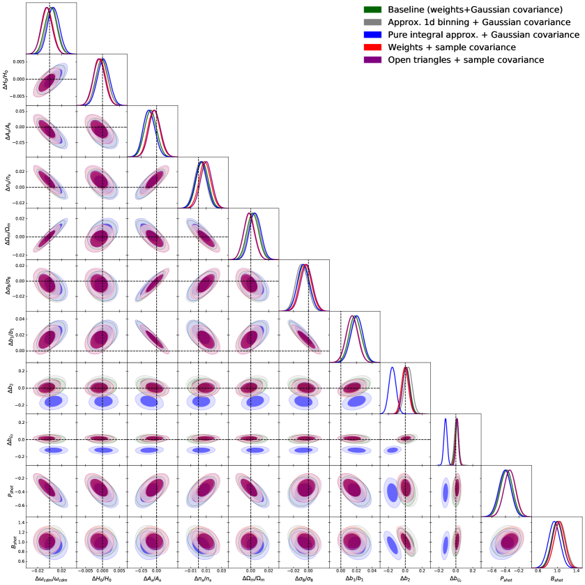
Eq. (A.2) is not exact because it was derived from the integral expression (3.26), which is approximate on its own. But we can still use it as an alternative prescription for the binning effects that will allow us to assess the systematic error of our baseline discreteness weight method. The two methods can be compared in Fig. 8, “Baseline” vs. “Approx 1d binning.” We can clearly see that they yield almost identical results. This validates our discreteness weight approach adopted in the main analysis. In this plot, we also show results from the “Pure integral approximation” obtained from the bispectrum model with the integral approximation but without discreteness weights or any additional corrections. This prescription leads to significant biases in the recovery of quadratic bias parameter $b_{2}$ and $b_{\mathcal{G}_{2}}$.

Figure 8: Triangle plots and 1d marginalized posteriors of cosmological and nuisance parameters from the following analyses that differ by the real space bispectrum likelihood treatments: baseline (Gaussian covariance + discretness weights), approximate 1d binning, integral approximation for binning without additional binning corrections (+ Gaussian covariance for the last two cases); likelihood based on the bispectrum sample covariance (discreteness weights), and the likelihood that includes the extra open triangles (+ sample covariance).

Appendix B Impact of Open Triangles

In principle, we could also include in our analysis the open triangles, i.e. the triangle bins that do not satisfy $|k_{3}-k_{2}|<k_{1}<k_{3}+k_{2}$ at their centers. We refrained from doing so because of the reasons listed in the main text. In this Appendix we explicitly check that neglecting these triangles does not lead to any appreciable loss of information. We include these triangles in the analysis by adopting the approximate 1d binning scheme described above. We have found that the Gaussian covariance approximation is very inaccurate for them, and therefore use a diagonal sample covariance matrix in our likelihood. The sample covariance matrix approximation for “usual” closed triangle configurations is validated in the next section, showing that it leads to essentially the same results as our baseline Gaussian covariances.

The results of our analysis of the bispectrum likelihood including open triangles are shown in Fig. 8, which should be compared with the case “Weights + sample covariance.” We see that the posterior distribution in this case is almost identical to that of the usual sample covariance analysis without open triangles, which implies that they can safely neglected for the purposes of this paper.

Appendix C Covariance Matrix Tests

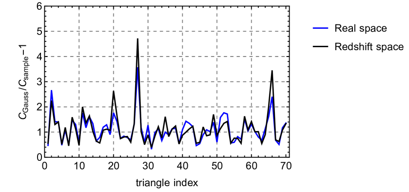
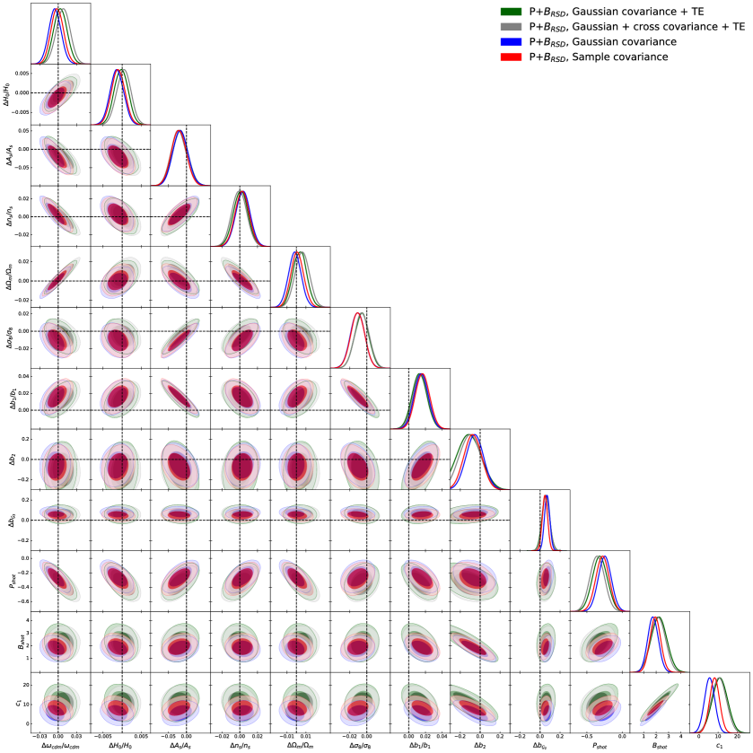
To test our baseline Gaussian covariance model, in this section we run our analysis with bispectrum likelihood based on sample covariance matrix estimators. The PT challenge suite consists of 10 boxes only, which means that the relative error on elements of the sample covariance in this case is around ${10}^{-1/2}\sim 30\%$. Since the sample covariance is not invertible for our baseline bispectrum data with 70 triangle bins, we will use only its diagonal part. This should still be a good approximation on large scales where the bispectrum covariance is dominated by the Gaussian diagonal contribution. The elements of our sample covariance normalized to the predictions of the Gaussian approximation are shown in Fig. 9. We see that the ratio is scattered around unity with most of the points dispersed within $\sim 50\%$ in accordance with the expected variance. However, we also observed several notable outliers. Nevertheless, the posterior distribution from the likelihood based on the sample covariance is almost identical to that of the baseline analysis, see Fig. 8 for the real space case and Fig. 10 for the redshift space case. We see that the main effect of the sample covariance is to shift the posterior distributions, but these shifts do not exceed $1\sigma$, which is an expected effect of the sampling noise in the covariance [27, 123].

C.1 Theoretical error and cross-covariance

Figure 9: Ratio of diagonal elements of the bispectrum covariance matrix computed in the Gaussian approximation and the sample covariance extracted from 10 PT challenge simulation boxes.

Figure 10: Triangle plots and 1d marginalized posteriors of cosmological and nuisance parameters from the joint redshift-space power spectrum and bispectrum likelihoods built with different covariance matrices: the Gaussian covariance, the Gaussian covariance including the theoretical error (TE), the Gaussian covariance including the theoretical error and the cross-covariance between the power spectrum and bispectrum, and the bispectrum sample covariance. In all cases we have used the discreteness weights and $k_{\rm max}=0.08~{}h\text{Mpc}^{-1}$ for the bispectrum likelihood.

TE covariance
Parameter	68% limits
$\Delta H_{0}/H_{0}$	$-0.0002\pm 0.0018$
$\Delta\omega_{cdm}/\omega_{cdm}$	$0.004\pm 0.011$
$\Delta A_{s}/A_{s}$	$-0.017\pm 0.021$
$\Delta n_{s}/n_{s}$	$0.0009\pm 0.0082$
$\Delta b_{1}/b_{1}$	$0.0128\pm 0.0089$
$\Delta b_{2}$	$-0.11\pm 0.12$
$\Delta b_{\mathcal{G}_{2}}$	$0.058\pm 0.038$
$P_{{shot}}$	$-0.32\pm 0.11$
$B_{{shot}}$	$2.36\pm 0.64$
$c_{1}$	$11.0\pm 4.0$
$\Delta\sigma_{8}/\sigma_{8}$	$-0.0059\pm 0.0083$
$\Delta\Omega_{m}/\Omega_{m}$	$0.0035\pm 0.0072$

TE + cross covariance
Parameter	68% limits
$\Delta H_{0}/H_{0}$	$0.0004\pm 0.0018$
$\Delta\omega_{cdm}/\omega_{cdm}$	$0.008\pm 0.011$
$\Delta A_{s}/A_{s}$	$-0.021\pm 0.021$
$\Delta n_{s}/n_{s}$	$-0.0006\pm 0.0084$
$\Delta b_{1}/b_{1}$	$0.0140\pm 0.0088$
$\Delta b_{2}$	$-0.10\pm 0.11$
$\Delta b_{\mathcal{G}_{2}}$	$0.059\pm 0.037$
$P_{{shot}}$	$-0.35\pm 0.10$
$B_{{shot}}$	$2.15\pm 0.59$
$c_{1}$	$10.4\pm 3.8$
$\Delta\sigma_{8}/\sigma_{8}$	$-0.0056\pm 0.0084$
$\Delta\Omega_{m}/\Omega_{m}$	$0.0061\pm 0.0075$

Table 3: 1d marginalized limits from analyses of the redshift space bispectrum monopole data at $k_{\rm max}=0.08~{}h\text{Mpc}^{-1}$ with two additional ingredients: the one-loop theoretical error (TE) bispectrum covariance (left table) and the TE bispectrum covariance plus the cross-covariance between the power spectrum multipoles and the bispectrum (right table).

We additionally check the stability of our results w.r.t. the inclusion of the theoretical error covariance to the bispectrum and the cross-covariance between the power spectrum multipoles and the bispectrum monopole.

The theoretical error covariance accounts for the imperfectness of the particular theoretical model that is used to fit the data. In the EFT approach theoretical calculations are done up to a fixed order on scales where higher order corrections are estimated to be negligible. A more systematic way to account for these corrections is to marginalize over their approximate shape dictated by the EFT power counting [4, 51]. This marginalization leads to a simple change of the covariance matrix by an additive correlated contribution. We incorporate the theoretical error covariance for the bispectrum following Ref. [4]. We use the following one-loop bispectrum theoretical error kernel

$$E_{B}(k_{1},k_{2},k_{3})=B_{\rm tree}(k_{1},k_{2},k_{3},z)D^{2}_{+}(z)\left(\frac{k_{1}+k_{2}+k_{3}}{3\times 0.23~{}h\text{Mpc}^{-1}}\right)^{3.3}\,,$$ (C.1)

whose amplitude is reduced by a factor of $3$ compared to Ref. [4]. We do so because the original envelope of Ref. [4] was calibrated to one-loop calculations at $k\sim 0.2~{}h\text{Mpc}^{-1}$ which is larger than our baseline cut $k_{\rm max}=0.08~{}h\text{Mpc}^{-1}$. We have checked that on these scales the original theory error kernel of Ref. [4] overestimates the actual size of one-loop matter bispectrum corrections, and therefore have accounted for it by multiplying this kernel by a factor $1/3$. Using Eq. (C.1), the theoretical error covariance can be written as

$$C^{B~{}(\rm TE)}_{TT^{\prime}}=E_{B}(k_{1},k_{2},k_{3})E_{B}(k^{\prime}_{1},k^{\prime}_{2},k^{\prime}_{3})\prod_{i=1}^{3}{\rm e}^{-\frac{(k_{i}-k^{\prime}_{i})}{2\delta k^{2}}}\,,$$ (C.2)

where the coherence scale $\delta k=0.1~{}h\text{Mpc}^{-1}$ following Refs. [6, 51]. The full covariance is given by

$$C^{B}_{TT^{\prime}}=C^{B~{}(\rm Gauss)}_{TT^{\prime}}+C^{B~{}(\rm TE)}_{TT^{\prime}}\,.$$ (C.3)

The result of our analysis of the bispectrum likelihood with the theoretical error covariance are presented in Fig. 10 and in Table 3. We see the inclusion of the theoretical error covariance leads to a moderate inflation of errorbars and insignificant shifts of some posteriors.

Finally, we include the cross-covariance between the power spectrum multipoles and the bispectrum monopole in our likelihood. We compute this cross-covariance in the tree-level approximation along the lines of Ref. [3], see Appendix F for more detail. The results of this analysis are displayed in the same Fig. 10 and Table 3. The impact of the cross-covariance is quite marginal – the posteriors are virtually identical to those of the previous analysis which treated the bispectrum and the power spectrum uncorrelated. This is consistent with common expectations that the cross-covariance is negligible on large scales [4, 6].

All in all, the analyses that we have carried out suggest that our baseline results are stable w.r.t. the choice of covariance matrices.

Appendix D Baseline power spectrum likelihood

Our baseline power spectrum likelihood consists of two pieces:

Redshift space multipoles

$\ell=0,2,4$ with $k_{\rm max}=0.14~{}h\text{Mpc}^{-1}$. We build the likelihood using the Gaussian approximation for the covariance matrix of these multipole moments. In the previous work [52] we have checked that the one-loop EFT model provides an accurate and unbiased fit to the data in this range.

Transverse moment (real space) power spectrum

in the range $0.14~{}h\text{Mpc}^{-1}<k<~{}0.4~{}h\text{Mpc}^{-1}$. We use the Gaussian covariance for real space part of the power spectrum likelihood.

Our power spectrum likelihood depends on the following nuisance parameters

$$\{b_{1},b_{2},b_{\mathcal{G}_{2}},b_{\Gamma_{3}},c_{0},c_{2},b_{4},a_{0},a_{2},P_{\rm shot}\}\,,$$ (D.1)

for which we assume following physically-motivated priors [41, 51, 50, 73]:

$$\begin{split}&b_{1}\in(1,4)\,,\quad b_{2}\sim\mathcal{N}(0,1^{2})\,,\quad b_{\mathcal{G}_{2}}\sim\mathcal{N}(0,1^{2})\,,\quad b_{\Gamma_{3}}\sim\mathcal{N}\left(\frac{23}{42}(b_{1}^{\rm fid}-1),1^{2}\right)\,,\\ &\frac{c_{0}}{(h^{-1}\text{Mpc})^{2}}\sim\mathcal{N}(4,10^{2})\,,\quad\frac{c_{0}}{(h^{-1}\text{Mpc})^{2}}\sim\mathcal{N}(20,20^{2})\,,\quad\frac{c_{4}}{(h^{-1}\text{Mpc})^{2}}\sim\mathcal{N}(-10,20^{2})\,,\\ &\frac{b_{4}}{(h^{-1}\text{Mpc})^{4}}\sim\mathcal{N}(500,500^{2})\,,\quad a_{0}\sim\mathcal{N}(0,1^{2})\,,\quad a_{2}\sim\mathcal{N}(0,1^{2})\,,\quad P_{\rm shot}\sim\mathcal{N}(0,1^{2})\,.\end{split}$$ (D.2)

Note that we use the following parametrization for the stochastic part of the redshift-space power spectrum,

$$P_{\rm stoch}(k,\mu)=\frac{1+P_{\rm shot}}{\bar{n}}+(a_{0}+a_{2}\mu^{2})\left(\frac{k}{0.45~{}h\text{Mpc}^{-1}}\right)^{2}\frac{1}{\bar{n}}\,.$$ (D.3)

Appendix E Real space power spectrum + bispectrum analysis

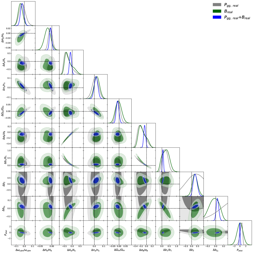
In this appendix we study the information content of clustering statistics purely in real space. We analyze the real space galaxy power spectrum of PT challenge simulation at $k_{\rm max}=0.2~{}h\text{Mpc}^{-1}$ and the real space bispectrum at $k_{\rm max}=0.08~{}h\text{Mpc}^{-1}$. The real space power spectrum case is very different from the redshift space one. In the absence of RSD the degeneracy between the linear galaxy bias $b_{1}$ and clustering amplitude $\sigma_{8}$ is largely unbroken. Moreover, the real space case does not capture the distance information, which should result in larger errorbars on $H_{0}$.

Our results are shown in Fig.11 and in table 4. The real space power spectrum data $P_{\text{gg, real}}$ is much less constraining than the dataset $[P_{0},P_{2},P_{4},Q_{0}]$ that we are using in our baseline redshift space power spectrum analysis. In particular, the constraints on $\omega_{\rm cdm},n_{s}$ and $H_{0}$ few times weaker, the limit on $\sigma_{8}$ is weaker by an order of magnitude. We can also see that the cosmological parameters’ posteriors from the bispectrum alone are comparable to the power spectrum ones. When we combine the two statistics the improvement is quite significant, e.g. the limit on $\sigma_{8}$ improves by a factor of four, the limit on $H_{0}$ by $30\%$.

Figure 11: Triangle plots and 1d marginalized posteriors of cosmological and nuisance parameters from the real space power spectra and bispectra data of the PT challenge simulation. For compactness, only linear and quadratic bias parameters are shown.

$P_{\text{gg, real}}$, real space
Parameter	68% limits
$\Delta H_{0}/H_{0}$	$-0.0058^{+0.0076}_{-0.0089}$
$\Delta\omega_{cdm}/\omega_{cdm}$	$-0.023^{+0.033}_{-0.040}$
$\Delta A_{s}/A_{s}$	$-0.29^{+0.13}_{-0.26}$
$\Delta n_{s}/n_{s}$	$0.011\pm 0.033$
$\Delta b_{1}/b_{1}$	$0.22^{+0.17}_{-0.19}$
$\Delta b_{2}$	$0.43\pm 0.91$
$\Delta b_{\mathcal{G}_{2}}$	$0.71^{+0.43}_{-0.55}$
$P_{{shot}}$	$0.38^{+0.57}_{-0.29}$
$\Delta\sigma_{8}/\sigma_{8}$	$-0.177^{+0.097}_{-0.16}$
$\Delta\Omega_{m}/\Omega_{m}$	$-0.008^{+0.015}_{-0.018}$

$B_{\rm real}$, real space
Parameter	68% limits
$\Delta H_{0}/H_{0}$	$-0.018\pm 0.013$
$\Delta\omega_{cdm}/\omega_{cdm}$	$-0.047\pm 0.028$
$\Delta A_{s}/A_{s}$	$-0.22^{+0.13}_{-0.31}$
$\Delta n_{s}/n_{s}$	$0.027\pm 0.029$
$\Delta b_{1}/b_{1}$	$0.25\pm 0.24$
$\Delta b_{2}$	$0.29^{+0.21}_{-0.24}$
$\Delta b_{\mathcal{G}_{2}}$	$-0.04^{+0.15}_{-0.11}$
$P_{{shot}}$	$0.0\pm 1.0$
$B_{{shot}}$	$0.87\pm 0.32$
$\Delta\sigma_{8}/\sigma_{8}$	$-0.148^{+0.091}_{-0.16}$
$\Delta\Omega_{m}/\Omega_{m}$	$-0.004^{+0.022}_{-0.025}$

$P_{\text{gg, real}}+B_{\rm real}$, real space
Parameter	68% limits
$\Delta H_{0}/H_{0}$	$-0.0054\pm 0.0047$
$\Delta\omega_{cdm}/\omega_{cdm}$	$-0.026\pm 0.020$
$\Delta A_{s}/A_{s}$	$-0.107^{+0.060}_{-0.068}$
$\Delta n_{s}/n_{s}$	$0.018\pm 0.019$
$\Delta b_{1}/b_{1}$	$0.071\pm 0.036$
$\Delta b_{2}$	$0.30^{+0.15}_{-0.18}$
$\Delta b_{\mathcal{G}_{2}}$	$0.046^{+0.029}_{-0.034}$
$P_{{shot}}$	$-0.05\pm 0.14$
$B_{{shot}}$	$0.96\pm 0.18$
$\Delta\sigma_{8}/\sigma_{8}$	$-0.066\pm 0.033$
$\Delta\Omega_{m}/\Omega_{m}$	$-0.011\pm 0.010$

Table 4: 1d marginalized limits from analyses of the real space power spectrum at $k_{\rm max}=0.20~{}h\text{Mpc}^{-1}$ and the real space bispectrum at $k_{\rm max}=0.08~{}h\text{Mpc}^{-1}$. For compactness, only linear and quadratic bias parameters are shown.

Appendix F Power spectrum and bispectrum covariances in perturbation theory

In this Appendix we calculate tree-level covariance matrices for the power spectrum and bispectrum. Let us start with the real-space estimators for the density power spectrum and bispectrum in the narrow bin approximation $\Delta k\ll k$ [20]

$$\begin{split}&\hat{P}(k_{i})=\int_{q\in k_{i}~{}\text{shell}}\frac{d^{3}q}{(2\pi)^{3}{\cal N}_{k}}~{}\delta(-{\bf q})\delta({\bf q})\,,\quad{\cal N}_{k}=4\pi k^{2}\Delta k\frac{V}{(2\pi)^{3}}\,.\\ &\hat{B}(k_{1},k_{2},k_{3})=\prod_{i=1}^{3}\int_{k_{i}}\frac{d^{3}q_{i}}{(2\pi)^{3}}~{}\frac{(2\pi)^{3}\delta^{(3)}({\bf q}_{123})}{N_{T}^{123}}\delta({\bf q}_{1})\delta({\bf q}_{2})\delta({\bf q}_{3})\,,\quad N^{123}_{T}=8\pi^{2}k_{1}k_{2}k_{3}\Delta k^{3}\frac{V^{2}}{(2\pi)^{6}}\,,\end{split}$$ (F.1)

Using the formulas from [99],

$$\begin{split}&\int r^{2}dr~{}j_{0}(k_{1}r)j_{0}(k_{2}r)j_{0}(k_{3}r)=\frac{\pi}{4}\,,\\ &\int_{k_{1}}\int_{k_{2}}\int_{k_{3}}[dq]^{3}~{}(2\pi)^{3}\delta^{(3)}({\bf q}_{123})=k_{1}k_{2}k_{3}\Delta k^{3}\frac{(4\pi)^{4}}{(2\pi)^{9}}\frac{\pi}{4}\,,\\ &\delta^{(3)}_{D}({\bf k}_{1}+{\bf k}_{2}+{\bf k}_{3})=\frac{1}{k_{1}k_{2}k_{3}}\delta^{(1)}_{D}\left(\cos({\bf k}_{1},{\bf k}_{2})-\frac{k_{3}^{2}-k_{1}^{2}-k_{1}^{2}}{2k_{1}k_{2}}\right)\delta^{(2)}_{D}\left(\hat{{\bf k}}_{3}-(\hat{{\bf k}}_{1}+\hat{{\bf k}}_{2})\right)\,,\end{split}$$ (F.2)

we can compute the auto-covariances of the estimators (F.1),

$$\begin{split}&C_{k_{i}k_{j}}=\frac{2}{\mathcal{N}_{k_{i}}}\delta_{ij}P^{2}(k_{i})\,,\quad C_{TT^{\prime}}=\frac{(2\pi)^{3}\pi s_{123}}{k_{1}k_{2}k_{3}\Delta k^{3}V}\delta_{TT^{\prime}}\prod_{i=1}^{3}P(k_{i})\,,\end{split}$$ (F.3)

where $s_{123}=~{}$6, 2 or 1 for equilateral, isosceles and general triangles. The cross-covariance $\langle P(k^{\prime})B(k_{1},k_{2},k_{3})\rangle$ is given by,

$$C_{k^{\prime}_{i}T}=\frac{2(2\pi)^{3}}{\mathcal{N}_{k^{\prime}_{i}}}\left(\delta_{ij_{1}}P(k^{\prime}_{i})B(k_{j_{1}},k_{j_{2}},k_{j_{3}})+\text{cycl.}\right)$$ (F.4)

It is straightforward to generalize these calculations to power spectrum multipole $\ell$ and the redshift-space bispectrum multipole $\ell^{\prime}$,

$$\begin{split}&\hat{P}_{\ell}(k_{i})=\int_{q\in k_{i}~{}\text{shell}}\frac{d^{3}q}{(2\pi)^{3}{\cal N}_{k}}~{}\delta_{0}(-{\bf q})\delta_{0}({{\bf q}})(2\ell+1)\mathcal{L}_{\ell}(\hat{{\bf z}}\cdot\hat{{\bf q}})\,,\\ &\hat{B}_{\ell^{\prime}}(k_{1},k_{2},k_{3})=(2\ell^{\prime}+1)\prod_{i=1}^{3}\int_{k_{i}}\frac{d^{3}q_{i}}{(2\pi)^{3}}~{}\frac{(2\pi)^{3}\delta^{(3)}_{D}({\bf q}_{123})}{N_{T}^{123}}\delta({\bf q}_{1})\delta({\bf q}_{2})\delta({\bf q}_{3})\mathcal{L}_{\ell^{\prime}}(\hat{{\bf z}}\cdot\hat{{\bf q}}_{1})\,,\end{split}$$ (F.5)

where $\delta_{0}({\bf k})=\delta({\bf k})(1+\beta\mu^{2})$ in the linear approximation [124], $\beta\equiv f/b_{1}$. In particular, this implies that the continuous part of the angle-averaged bispectrum auto-covariance would be modulated in redshift space by a form-factor

$$\int\frac{d\phi}{2\pi}\int_{0}^{1}d\mu~{}(1+\beta\mu^{2})^{2}(1+\beta\mu_{2}(\mu,\phi)^{2})^{2}(1+\beta\mu_{3}(\mu,\phi)^{2})^{2}\,.$$ (F.6)

Similarly, the cross-correlation between $P_{\ell}$ and $B_{0}$ is given by

$$\begin{split}&\langle P_{\ell}(k)B_{0}(k_{1},k_{2},k_{3})\rangle\\ &=\frac{2(2\pi)^{3}(2\ell+1)}{\mathcal{N}_{k}}\left(\delta_{kk_{1}}P(k)\int\frac{d\phi}{2\pi}\int_{0}^{1}d\mu~{}(1+\beta\mu^{2})^{2}\mathcal{L}_{\ell}(\mu)B({\bf k},{\bf k}_{2},{\bf k}_{3})+\text{cycl.}\right)\,.\end{split}$$ (F.7)

Appendix G Gaussian fingers-of-God exponent derivation

In this section we revisit the derivation of the Gaussian FoG exponent that is often used in the literature to motivate some phenomenological models for FoG, see e.g. [16]. Ref. [51] has explicitly shown that this model completely fails to capture the behaviour seen in high quality dark matter redshift space simulations. Nevertheless, it would be of some interest to see when the Gaussian FoG model breaks down at the mathematical level. Let us consider the redshift space mapping,

$$\delta^{(z)}({\bf k})=\int d^{3}x~{}{\rm e}^{i{\bf k}{\bf x}+i\mathcal{H}^{-1}k_{z}v_{z}({\bf x})}(\delta({\bf x})+1)-(2\pi)^{3}\delta^{(3)}_{D}({\bf k})$$ (G.1)

Now we split the velocity field into the long and short wavelength components,

$$v_{i}=v^{L}_{i}+v^{S}_{i}\,,$$ (G.2)

where $v^{L}$ is correlated with the density field on large scales and $v^{S}$ is the short-scale contribution generated by the non-perturbative effects such as virialization. A common assumption is that this part is fully uncorrelated with the perturbative long wavelength density field. Taylor-expanding the exponent over its perturbative part we have

$$\delta^{(z)}({\bf k})=\int d^{3}x~{}{\rm e}^{i{\bf k}{\bf x}+i\mathcal{H}^{-1}k_{z}v^{S}_{z}({\bf x})}(\delta({\bf x})+i\mathcal{H}^{-1}k_{z}v^{L}_{z}({\bf x}))\,,$$ (G.3)

where we have neglected terms which have support only around ${\bf k}=0$. In what follows we restrict ourselves to the tree-level order for the perturbative part, in which case the velocity field can be expressed as

$$v^{L}_{i}=-f\mathcal{H}\frac{\partial_{i}\delta^{L}_{m}}{\Delta}\quad\Rightarrow\quad i\mathcal{H}^{-1}k_{z}v^{L}_{i}({\bf k})=f\mu^{2}\delta^{L}_{m}({\bf k})\,.$$ (G.4)

In order to reproduce the Gaussian FoG exponent, we need to assume the short scale velocity field is Gaussian distributed, and its two point correlation function has a finite support on short scales,

$$\begin{split}\langle v_{i}({\bf x})v_{j}({\bf x}^{\prime})\rangle=\delta_{ij}\mathcal{H}^{2}\sigma^{2}_{v}\quad\text{for}\quad{\bf x}={\bf x}^{\prime}\quad\text{and}\quad 0\quad\text{otherwise}.\end{split}$$ (G.5)

Clearly, this assumption cannot be justified within the EFT approach, which requires that the short-scale averages should depend on all possible operators involving low-energy degrees of freedom compatible with IR symmetries of large-scale structure [39]. Nevertheless, if we proceed using the cumulant expansion theorem

$$\langle\exp\{iX\}\rangle=\exp\left\{\sum_{N=1}^{\infty}\frac{i^{N}}{N!}\langle X^{N}\rangle_{c}\right\}\,,$$ (G.6)

we find the power spectrum in redshift space given by

$$\begin{split}\langle\delta^{(z)}({\bf k})\delta^{(z)}({\bf k}^{\prime})\rangle=(2\pi)^{3}\delta_{D}^{(3)}({\bf k}+{\bf k}^{\prime})~{}{\rm e}^{-\sigma_{v}^{2}\mu^{2}k^{2}}P_{\rm Kaiser}(k)\,,\end{split}$$ (G.7)

where

$$P_{\rm Kaiser}(k)=(b_{1}+f\mu^{2})^{2}P(k)+\frac{1}{\bar{n}}\,.$$ (G.8)

For the redshift space bispectrum we have

$$\begin{split}&\langle\delta^{(z)}({\bf k}_{1})\delta^{(z)}({\bf k}_{2})\delta^{(z)}({\bf k}_{3})\rangle=(2\pi)^{3}\delta_{D}^{(3)}({\bf k}_{123})~{}{\rm e}^{-\frac{\sigma_{v}^{2}}{2}\sum_{a=1}^{3}\mu_{a}^{2}k_{a}^{2}}B_{\rm tree}({\bf k}_{1},{\bf k}_{2},{\bf k}_{3})\,,\end{split}$$ (G.9)

which would formally coincide with the leading order EFT expression used in this work if we Taylor expand the damping exponent and identify

$$c_{1}=\frac{(k_{\rm NL}^{r})^{2}}{2}\sigma_{v}^{2}b_{1}\,,\quad c_{2}=\frac{(k_{\rm NL}^{r})^{2}}{2}\sigma_{v}^{2}f\,.$$ (G.10)

References

- [1] P. J. E. Peebles, The large-scale structure of the universe. 1980.
- [2] R. Scoccimarro, The bispectrum: from theory to observations, Astrophys. J. 544 (2000) 597 [astro-ph/0004086].
- [3] E. Sefusatti, M. Crocce, S. Pueblas and R. Scoccimarro, Cosmology and the Bispectrum, Phys. Rev. D74 (2006) 023522 [astro-ph/0604505].
- [4] T. Baldauf, M. Mirbabayi, M. Simonović and M. Zaldarriaga, LSS constraints with controlled theoretical uncertainties, 1602.00674.
- [5] V. Yankelevich and C. Porciani, Cosmological information in the redshift-space bispectrum, Mon. Not. Roy. Astron. Soc. 483 (2019) 2078 [1807.07076].
- [6] A. Chudaykin and M. M. Ivanov, Measuring neutrino masses with large-scale structure: Euclid forecast with controlled theoretical error, JCAP 11 (2019) 034 [1907.06666].
- [7] C. Hahn, F. Villaescusa-Navarro, E. Castorina and R. Scoccimarro, Constraining with the bispectrum. Part I. Breaking parameter degeneracies, JCAP 03 (2020) 040 [1909.11107].
- [8] C. Hahn and F. Villaescusa-Navarro, Constraining with the bispectrum. Part II. The information content of the galaxy bispectrum monopole, JCAP 04 (2021) 029 [2012.02200].
- [9] Y. Welling, D. van der Woude and E. Pajer, Lifting Primordial Non-Gaussianity Above the Noise, JCAP 08 (2016) 044 [1605.06426].
- [10] A. Moradinezhad Dizgah, M. Biagetti, E. Sefusatti, V. Desjacques and J. Noreña, Primordial Non-Gaussianity from Biased Tracers: Likelihood Analysis of Real-Space Power Spectrum and Bispectrum, JCAP 05 (2021) 015 [2010.14523].
- [11] P. J. E. Peebles and E. J. Groth, Statistical analysis of catalogs of extragalactic objects. V. Three-point correlation function for the galaxy distribution in the Zwicky catalog., Astrophys. J. 196 (1975) 1.
- [12] E. J. Groth and P. J. E. Peebles, Statistical analysis of catalogs of extragalactic objects. VII. Two- and three-point correlation functions for the high-resolution Shane-Wirtanen catalog of galaxies., Astrophys. J. 217 (1977) 385.
- [13] R. Scoccimarro, H. A. Feldman, J. N. Fry and J. A. Frieman, The Bispectrum of IRAS redshift catalogs, Astrophys. J. 546 (2001) 652 [astro-ph/0004087].
- [14] H. A. Feldman, J. A. Frieman, J. N. Fry and R. Scoccimarro, Constraints on galaxy bias, matter density, and primordial non-gausianity from the PSCz galaxy redshift survey, Phys. Rev. Lett. 86 (2001) 1434 [astro-ph/0010205].
- [15] WiggleZ collaboration, F. A. Marin et al., The WiggleZ Dark Energy Survey: constraining galaxy bias and cosmic growth with 3-point correlation functions, Mon. Not. Roy. Astron. Soc. 432 (2013) 2654 [1303.6644].
- [16] H. Gil-Marín, J. Noreña, L. Verde, W. J. Percival, C. Wagner, M. Manera et al., The power spectrum and bispectrum of SDSS DR11 BOSS galaxies – I. Bias and gravity, Mon. Not. Roy. Astron. Soc. 451 (2015) 539 [1407.5668].
- [17] H. Gil-Marín, L. Verde, J. Noreña, A. J. Cuesta, L. Samushia, W. J. Percival et al., The power spectrum and bispectrum of SDSS DR11 BOSS galaxies – II. Cosmological interpretation, Mon. Not. Roy. Astron. Soc. 452 (2015) 1914 [1408.0027].
- [18] H. Gil-Marín, W. J. Percival, L. Verde, J. R. Brownstein, C.-H. Chuang, F.-S. Kitaura et al., The clustering of galaxies in the SDSS-III Baryon Oscillation Spectroscopic Survey: RSD measurement from the power spectrum and bispectrum of the DR12 BOSS galaxies, Mon. Not. Roy. Astron. Soc. 465 (2017) 1757 [1606.00439].
- [19] Z. Slepian et al., The large-scale three-point correlation function of the SDSS BOSS DR12 CMASS galaxies, Mon. Not. Roy. Astron. Soc. 468 (2017) 1070 [1512.02231].
- [20] R. Scoccimarro, Fast Estimators for Redshift-Space Clustering, Phys. Rev. D 92 (2015) 083532 [1506.02729].
- [21] O. H. E. Philcox and D. J. Eisenstein, Computing the Small-Scale Galaxy Power Spectrum and Bispectrum in Configuration-Space, Mon. Not. Roy. Astron. Soc. 492 (2020) 1214 [1912.01010].
- [22] O. H. E. Philcox and D. J. Eisenstein, Estimating Covariance Matrices for Two- and Three-Point Correlation Function Moments in Arbitrary Survey Geometries, Mon. Not. Roy. Astron. Soc. 490 (2019) 5931 [1910.04764].
- [23] O. H. E. Philcox, A faster Fourier transform? Computing small-scale power spectra and bispectra for cosmological simulations in time, Mon. Not. Roy. Astron. Soc. 501 (2021) 4004 [2005.01739].
- [24] O. H. E. Philcox, Z. Slepian, J. Hou, C. Warner, R. N. Cahn and D. J. Eisenstein, ENCORE: Estimating Galaxy -point Correlation Functions in Time, 2105.08722.
- [25] E. Gaztanaga and R. Scoccimarro, The 3-point function in large scale structure: Redshift distortions and galaxy bias, Mon. Not. Roy. Astron. Soc. 361 (2005) 824 [astro-ph/0501637].
- [26] D. Gualdi, H. Gil-Marín, R. L. Schuhmann, M. Manera, B. Joachimi and O. Lahav, Enhancing BOSS bispectrum cosmological constraints with maximal compression, Mon. Not. Roy. Astron. Soc. 484 (2019) 3713 [1806.02853].
- [27] O. H. E. Philcox, M. M. Ivanov, M. Zaldarriaga, M. Simonovic and M. Schmittfull, Fewer Mocks and Less Noise: Reducing the Dimensionality of Cosmological Observables with Subspace Projections, Phys. Rev. D 103 (2021) 043508 [2009.03311].
- [28] F.-S. Kitaura et al., The clustering of galaxies in the SDSS-III Baryon Oscillation Spectroscopic Survey: mock galaxy catalogues for the BOSS Final Data Release, Mon. Not. Roy. Astron. Soc. 456 (2016) 4156 [1509.06400].
- [29] F.-S. Kitaura, H. Gil-Marín, C. Scoccola, C.-H. Chuang, V. Müller, G. Yepes et al., Constraining the halo bispectrum in real and redshift space from perturbation theory and non-linear stochastic bias, Mon. Not. Roy. Astron. Soc. 450 (2015) 1836 [1407.1236].
- [30] R. Takahashi, T. Nishimichi, T. Namikawa, A. Taruya, I. Kayo, K. Osato et al., Fitting the Nonlinear Matter Bispectrum by the Halofit Approach, The Astrophysical Journal 895 (2020) 113 [1911.07886].
- [31] K. Heitmann, D. Higdon, M. White, S. Habib, B. J. Williams and C. Wagner, The Coyote Universe II: Cosmological Models and Precision Emulation of the Nonlinear Matter Power Spectrum, Astrophys. J. 705 (2009) 156 [0902.0429].
- [32] T. Nishimichi, M. Takada, R. Takahashi, K. Osato, M. Shirasaki, T. Oogi et al., Dark Quest. I. Fast and Accurate Emulation of Halo Clustering Statistics and Its Application to Galaxy Clustering, The Astrophysical Journal 884 (2019) 29 [1811.09504].
- [33] Y. Kobayashi, T. Nishimichi, M. Takada, R. Takahashi and K. Osato, Accurate emulator for the redshift-space power spectrum of dark matter halos and its application to galaxy power spectrum, Phys. Rev. D 102 (2020) 063504 [2005.06122].
- [34] A. Schneider, R. Teyssier, D. Potter, J. Stadel, J. Onions, D. S. Reed et al., Matter power spectrum and the challenge of percent accuracy, JCAP 1604 (2016) 047 [1503.05920].
- [35] J. N. Fry, The Galaxy correlation hierarchy in perturbation theory, Astrophys. J. 279 (1984) 499.
- [36] R. Scoccimarro and J. Frieman, Loop corrections in nonlinear cosmological perturbation theory, Astrophys. J. Suppl. 105 (1996) 37 [astro-ph/9509047].
- [37] R. Scoccimarro, S. Colombi, J. N. Fry, J. A. Frieman, E. Hivon and A. Melott, Nonlinear evolution of the bispectrum of cosmological perturbations, Astrophys. J. 496 (1998) 586 [astro-ph/9704075].
- [38] R. Scoccimarro, H. M. P. Couchman and J. A. Frieman, The Bispectrum as a Signature of Gravitational Instability in Redshift-Space, Astrophys. J. 517 (1999) 531 [astro-ph/9808305].
- [39] D. Baumann, A. Nicolis, L. Senatore and M. Zaldarriaga, Cosmological Non-Linearities as an Effective Fluid, JCAP 1207 (2012) 051 [1004.2488].
- [40] J. J. M. Carrasco, M. P. Hertzberg and L. Senatore, The Effective Field Theory of Cosmological Large Scale Structures, JHEP 09 (2012) 082 [1206.2926].
- [41] A. Chudaykin, M. M. Ivanov, O. H. E. Philcox and M. Simonović, Nonlinear perturbation theory extension of the Boltzmann code CLASS, Phys. Rev. D 102 (2020) 063533 [2004.10607].
- [42] G. D’Amico, L. Senatore and P. Zhang, Limits on CDM from the EFTofLSS with the PyBird code, JCAP 01 (2021) 006 [2003.07956].
- [43] S.-F. Chen, Z. Vlah, E. Castorina and M. White, Redshift-Space Distortions in Lagrangian Perturbation Theory, JCAP 03 (2021) 100 [2012.04636].
- [44] BOSS collaboration, S. Alam et al., The clustering of galaxies in the completed SDSS-III Baryon Oscillation Spectroscopic Survey: cosmological analysis of the DR12 galaxy sample, Mon. Not. Roy. Astron. Soc. 470 (2017) 2617 [1607.03155].
- [45] M. M. Ivanov, M. Simonović and M. Zaldarriaga, Cosmological Parameters from the BOSS Galaxy Power Spectrum, JCAP 05 (2020) 042 [1909.05277].
- [46] G. D’Amico, J. Gleyzes, N. Kokron, D. Markovic, L. Senatore, P. Zhang et al., The Cosmological Analysis of the SDSS/BOSS data from the Effective Field Theory of Large-Scale Structure, 1909.05271.
- [47] M. M. Ivanov, M. Simonović and M. Zaldarriaga, Cosmological Parameters and Neutrino Masses from the Final Planck and Full-Shape BOSS Data, Phys. Rev. D 101 (2020) 083504 [1912.08208].
- [48] M. M. Ivanov, E. McDonough, J. C. Hill, M. Simonović, M. W. Toomey, S. Alexander et al., Constraining Early Dark Energy with Large-Scale Structure, Phys. Rev. D 102 (2020) 103502 [2006.11235].
- [49] G. D’Amico, L. Senatore, P. Zhang and H. Zheng, The Hubble Tension in Light of the Full-Shape Analysis of Large-Scale Structure Data, 2006.12420.
- [50] A. Chudaykin, K. Dolgikh and M. M. Ivanov, Constraints on the curvature of the Universe and dynamical dark energy from the Full-shape and BAO data, Phys. Rev. D 103 (2021) 023507 [2009.10106].
- [51] A. Chudaykin, M. M. Ivanov and M. Simonović, Optimizing large-scale structure data analysis with the theoretical error likelihood, Phys. Rev. D 103 (2021) 043525 [2009.10724].
- [52] T. Nishimichi, G. D’Amico, M. M. Ivanov, L. Senatore, M. Simonović, M. Takada et al., Blinded challenge for precision cosmology with large-scale structure: results from effective field theory for the redshift-space galaxy power spectrum, Phys. Rev. D 102 (2020) 123541 [2003.08277].
- [53] P. Valageas and T. Nishimichi, Combining perturbation theories with halo models for the matter bispectrum, Astronomy & Astrophysics 532 (2011) A4 [1102.0641].
- [54] R. E. Angulo, S. Foreman, M. Schmittfull and L. Senatore, The One-Loop Matter Bispectrum in the Effective Field Theory of Large Scale Structures, JCAP 1510 (2015) 039 [1406.4143].
- [55] T. Baldauf, L. Mercolli, M. Mirbabayi and E. Pajer, The Bispectrum in the Effective Field Theory of Large Scale Structure, JCAP 1505 (2015) 007 [1406.4135].
- [56] D. Bertolini, K. Schutz, M. P. Solon and K. M. Zurek, The Trispectrum in the Effective Field Theory of Large Scale Structure, JCAP 06 (2016) 052 [1604.01770].
- [57] A. Eggemeier, R. Scoccimarro and R. E. Smith, Bias Loop Corrections to the Galaxy Bispectrum, 1812.03208.
- [58] A. Taruya, T. Nishimichi and D. Jeong, Grid-based calculation for perturbation theory of large-scale structure, Phys. Rev. D 98 (2018) 103532 [1807.04215].
- [59] K. Osato, T. Nishimichi, A. Taruya and F. Bernardeau, Implementing spectra response function approaches for fast calculation of power spectra and bispectra, arXiv e-prints (2021) arXiv:2107.04275 [2107.04275].
- [60] L. Senatore and M. Zaldarriaga, Redshift Space Distortions in the Effective Field Theory of Large Scale Structures, 1409.1225.
- [61] M. Lewandowski, L. Senatore, F. Prada, C. Zhao and C.-H. Chuang, EFT of large scale structures in redshift space, Phys. Rev. D 97 (2018) 063526 [1512.06831].
- [62] A. Perko, L. Senatore, E. Jennings and R. H. Wechsler, Biased Tracers in Redshift Space in the EFT of Large-Scale Structure, 1610.09321.
- [63] L. Senatore, Bias in the Effective Field Theory of Large Scale Structures, JCAP 1511 (2015) 007 [1406.7843].
- [64] R. Angulo, M. Fasiello, L. Senatore and Z. Vlah, On the Statistics of Biased Tracers in the Effective Field Theory of Large Scale Structures, JCAP 1509 (2015) 029 [1503.08826].
- [65] V. Assassi, D. Baumann, D. Green and M. Zaldarriaga, Renormalized Halo Bias, JCAP 1408 (2014) 056 [1402.5916].
- [66] M. Mirbabayi, F. Schmidt and M. Zaldarriaga, Biased Tracers and Time Evolution, JCAP 1507 (2015) 030 [1412.5169].
- [67] V. Desjacques, D. Jeong and F. Schmidt, Large-Scale Galaxy Bias, Phys. Rept. 733 (2018) 1 [1611.09787].
- [68] V. Desjacques, D. Jeong and F. Schmidt, The Galaxy Power Spectrum and Bispectrum in Redshift Space, JCAP 1812 (2018) 035 [1806.04015].
- [69] D. Blas, M. Garny, M. M. Ivanov and S. Sibiryakov, Time-Sliced Perturbation Theory II: Baryon Acoustic Oscillations and Infrared Resummation, JCAP 1607 (2016) 028 [1605.02149].
- [70] M. M. Ivanov and S. Sibiryakov, Infrared Resummation for Biased Tracers in Redshift Space, JCAP 1807 (2018) 053 [1804.05080].
- [71] A. Taruya, T. Nishimichi and D. Jeong, Grid-based calculations of redshift-space matter fluctuations from perturbation theory: UV sensitivity and convergence at the field level, arXiv e-prints (2021) arXiv:2109.06734 [2109.06734].
- [72] C. Alcock and B. Paczynski, An evolution free test for non-zero cosmological constant, Nature 281 (1979) 358.
- [73] M. M. Ivanov, O. H. E. Philcox, M. Simonović, M. Zaldarriaga, T. Nishimichi and M. Takada, Cosmological constraints without fingers of God, 2110.00006.
- [74] A. J. S. Hamilton and M. Tegmark, The Real space power spectrum of the PSCz survey from 0.01 to 300 h Mpc**-1, Mon. Not. Roy. Astron. Soc. 330 (2002) 506 [astro-ph/0008392].
- [75] SDSS collaboration, M. Tegmark et al., The 3-D power spectrum of galaxies from the SDSS, Astrophys. J. 606 (2004) 702 [astro-ph/0310725].
- [76] R. Scoccimarro, Redshift-space distortions, pairwise velocities and nonlinearities, Phys. Rev. D70 (2004) 083007 [astro-ph/0407214].
- [77] F. Bernardeau, S. Colombi, E. Gaztanaga and R. Scoccimarro, Large scale structure of the universe and cosmological perturbation theory, Phys. Rept. 367 (2002) 1 [astro-ph/0112551].
- [78] M. Schmittfull, T. Baldauf and U. Seljak, Near optimal bispectrum estimators for large-scale structure, Phys. Rev. D91 (2015) 043530 [1411.6595].
- [79] R. Casas-Miranda, H. J. Mo, R. K. Sheth and G. Boerner, On the Distribution of Haloes, Galaxies and Mass, Mon. Not. Roy. Astron. Soc. 333 (2002) 730 [astro-ph/0105008].
- [80] T. Baldauf, U. Seljak, R. E. Smith, N. Hamaus and V. Desjacques, Halo stochasticity from exclusion and nonlinear clustering, Phys. Rev. D 88 (2013) 083507 [1305.2917].
- [81] T. Baldauf, S. Codis, V. Desjacques and C. Pichon, Peak exclusion, stochasticity and convergence of perturbative bias expansions in 1+1 gravity, Mon. Not. Roy. Astron. Soc. 456 (2016) 3985 [1510.09204].
- [82] M. Schmittfull, M. Simonović, V. Assassi and M. Zaldarriaga, Modeling Biased Tracers at the Field Level, Phys. Rev. D 100 (2019) 043514 [1811.10640].
- [83] J. C. Jackson, Fingers of God: A critique of Rees’ theory of primoridal gravitational radiation, Mon. Not. Roy. Astron. Soc. 156 (1972) 1P [0810.3908].
- [84] Z. Vlah and M. White, Exploring redshift-space distortions in large-scale structure, JCAP 1903 (2019) 007 [1812.02775].
- [85] S.-F. Chen, Z. Vlah and M. White, Consistent Modeling of Velocity Statistics and Redshift-Space Distortions in One-Loop Perturbation Theory, JCAP 07 (2020) 062 [2005.00523].
- [86] M. M. Ivanov, Cosmological constraints from the power spectrum of eBOSS emission line galaxies, 2106.12580.
- [87] L. Senatore and M. Zaldarriaga, The IR-resummed Effective Field Theory of Large Scale Structures, JCAP 1502 (2015) 013 [1404.5954].
- [88] T. Baldauf, M. Mirbabayi, M. Simonović and M. Zaldarriaga, Equivalence Principle and the Baryon Acoustic Peak, Phys. Rev. D92 (2015) 043514 [1504.04366].
- [89] D. Blas, M. Garny, M. M. Ivanov and S. Sibiryakov, Time-Sliced Perturbation Theory for Large Scale Structure I: General Formalism, JCAP 1607 (2016) 052 [1512.05807].
- [90] Z. Vlah, M. White and A. Aviles, A Lagrangian effective field theory, JCAP 09 (2015) 014 [1506.05264].
- [91] Z. Vlah, U. Seljak, M. Y. Chu and Y. Feng, Perturbation theory, effective field theory, and oscillations in the power spectrum, JCAP 1603 (2016) 057 [1509.02120].
- [92] M. Crocce and R. Scoccimarro, Nonlinear Evolution of Baryon Acoustic Oscillations, Phys. Rev. D77 (2008) 023533 [0704.2783].
- [93] A. Vasudevan, M. M. Ivanov, S. Sibiryakov and J. Lesgourgues, Time-sliced perturbation theory with primordial non-Gaussianity and effects of large bulk flows on inflationary oscillating features, JCAP 09 (2019) 037 [1906.08697].
- [94] Y.-S. Song, A. Taruya and A. Oka, Cosmology with anisotropic galaxy clustering from the combination of power spectrum and bispectrum, JCAP 1508 (2015) 007 [1502.03099].
- [95] F. Bernardeau, M. Crocce and R. Scoccimarro, Constructing Regularized Cosmic Propagators, Phys. Rev. D 85 (2012) 123519 [1112.3895].
- [96] A. Oddo, E. Sefusatti, C. Porciani, P. Monaco and A. G. Sánchez, Toward a robust inference method for the galaxy bispectrum: likelihood function and model selection, JCAP 03 (2020) 056 [1908.01774].
- [97] E. Sefusatti, M. Crocce and V. Desjacques, The matter bispectrum in N-body simulations with non-Gaussian initial conditions, MNRAS 406 (2010) 1014 [1003.0007].
- [98] A. Eggemeier, R. Scoccimarro, R. E. Smith, M. Crocce, A. Pezzotta and A. G. Sánchez, Testing one-loop galaxy bias: joint analysis of power spectrum and bispectrum, 2102.06902.
- [99] R. Mehrem, J. T. Londergan and M. H. Macfarlane, Analytic expressions for integrals of products of spherical Bessel functions, J. Phys. A 24 (1991) 1435.
- [100] T. Brinckmann and J. Lesgourgues, MontePython 3: boosted MCMC sampler and other features, Phys. Dark Univ. 24 (2019) 100260 [1804.07261].
- [101] B. Audren, J. Lesgourgues, K. Benabed and S. Prunet, Conservative Constraints on Early Cosmology: an illustration of the Monte Python cosmological parameter inference code, JCAP 1302 (2013) 001 [1210.7183].
- [102] A. Lewis, GetDist: a Python package for analysing Monte Carlo samples, 1910.13970.
- [103] D. Blas, J. Lesgourgues and T. Tram, The Cosmic Linear Anisotropy Solving System (CLASS) II: Approximation schemes, JCAP 1107 (2011) 034 [1104.2933].
- [104] M. M. Ivanov, Y. Ali-Haïmoud and J. Lesgourgues, H0 tension or T0 tension?, Phys. Rev. D 102 (2020) 063515 [2005.10656].
- [105] M. M. Abidi and T. Baldauf, Cubic Halo Bias in Eulerian and Lagrangian Space, JCAP 1807 (2018) 029 [1802.07622].
- [106] A. Eggemeier, R. Scoccimarro, M. Crocce, A. Pezzotta and A. G. Sánchez, Testing one-loop galaxy bias: Power spectrum, Phys. Rev. D 102 (2020) 103530 [2006.09729].
- [107] T. Lazeyras, C. Wagner, T. Baldauf and F. Schmidt, Precision measurement of the local bias of dark matter halos, JCAP 1602 (2016) 018 [1511.01096].
- [108] T. Lazeyras and F. Schmidt, Beyond LIMD bias: a measurement of the complete set of third-order halo bias parameters, JCAP 1809 (2018) 008 [1712.07531].
- [109] A. Barreira, T. Lazeyras and F. Schmidt, Galaxy bias from forward models: linear and second-order bias of IllustrisTNG galaxies, 2105.02876.
- [110] S. Pueblas and R. Scoccimarro, Generation of Vorticity and Velocity Dispersion by Orbit Crossing, Phys. Rev. D80 (2009) 043504 [0809.4606].
- [111] M. Schmittfull, M. Simonović, M. M. Ivanov, O. H. E. Philcox and M. Zaldarriaga, Modeling Galaxies in Redshift Space at the Field Level, 2012.03334.
- [112] R. E. Smith, R. K. Sheth and R. Scoccimarro, An analytic model for the bispectrum of galaxies in redshift space, Phys. Rev. D 78 (2008) 023523 [0712.0017].
- [113] O. H. E. Philcox, M. M. Ivanov, M. Simonović and M. Zaldarriaga, Combining Full-Shape and BAO Analyses of Galaxy Power Spectra: A 1.6\% CMB-independent constraint on H0, JCAP 05 (2020) 032 [2002.04035].
- [114] O. H. E. Philcox, Cosmology without window functions: Quadratic estimators for the galaxy power spectrum, Phys. Rev. D 103 (2021) 103504 [2012.09389].
- [115] O. H. E. Philcox, Cosmology Without Window Functions: Cubic Estimators for the Galaxy Bispectrum, 2107.06287.
- [116] M. M. Ivanov and O. H. E. Philcox, to appear, .
- [117] E. Di Valentino et al., Cosmology Intertwined III: and , 2008.11285.
- [118] DESI collaboration, A. Aghamousa et al., The DESI Experiment Part I: Science,Targeting, and Survey Design, 1611.00036.
- [119] EUCLID collaboration, R. Laureijs et al., Euclid Definition Study Report, 1110.3193.
- [120] L. Amendola et al., Cosmology and fundamental physics with the Euclid satellite, Living Rev. Rel. 21 (2018) 2 [1606.00180].
- [121] A. de Mattia et al., The Completed SDSS-IV extended Baryon Oscillation Spectroscopic Survey: measurement of the BAO and growth rate of structure of the emission line galaxy sample from the anisotropic power spectrum between redshift 0.6 and 1.1, Mon. Not. Roy. Astron. Soc. 501 (2021) 5616 [2007.09008].
- [122] A. Oddo, F. Rizzo, E. Sefusatti, C. Porciani and P. Monaco, Cosmological parameters from the likelihood analysis of the galaxy power spectrum and bispectrum in real space, 2108.03204.
- [123] D. Wadekar, M. M. Ivanov and R. Scoccimarro, Cosmological constraints from BOSS with analytic covariance matrices, Phys. Rev. D 102 (2020) 123521 [2009.00622].
- [124] N. Kaiser, Clustering in real space and in redshift space, Mon. Not. Roy. Astron. Soc. 227 (1987) 1.