Activation Landscapes as a Topological Summary of Neural Network Performance

Abstract

We use topological data analysis (TDA) to study how data transforms as it passes through successive layers of a deep neural network (DNN). We compute the persistent homology of the activation data for each layer of the network and summarize this information using persistence landscapes. The resulting feature map provides both an informative visualization of the network and a kernel for statistical analysis and machine learning. We observe that the topological complexity often increases with training and that the topological complexity does not decrease with each layer.

I Introduction

Deep neural networks (DNNs) have become an indispensable tool for handling and analyzing large amounts of data. While they have been extremely successful for classifying complex data sets, the way in which they make decisions is often opaque. We will use topological data analysis (TDA) to provide a new summary of a DNN which is designed to illuminate aspects of DNN learning and performance. We focus on how DNNs transform the topology of the input data manifold and how training affects these topological transformations. To this end, we use a TDA method, persistence landscapes, to provide a feature map and kernel for the activations of each of the layers in a DNN and we use this method to summarize changes in the DNN during learning.

I-A Topological Data Analysis

Large data sets can exhibit highly complicated topological and geometric structure that is both difficult to summarize and crucial for understanding the data. Topological data analysis (TDA) uses methods based on algebraic topology to quantify and study the shape of data. One of the primary tools of TDA, persistent homology, gives a complete summary of the homology of a one-parameter family of topological spaces [14, 48]. As an important application, a collection of points in Euclidean space may be used to produce a one-parameter family consisting of unions of balls centered at these points of uniform increasing radius. There are a number of efficient implementations for computing persistent homology [29, 31, 5, 4] A variant, called local homology, has been used to learn the stratification of data [28, 32, 37, 6].

I-B Deep Neural Networks

Deep Neural Networks (DNNs) are overparametrized models with multiple layers and have been shown to be effective for a variety of machine learning tasks, especially for structured data such as images or text [16]. Examples of DNN successes include applications in biology [12, 27, 1], chemistry [26], engineering [33], medicine [11], physics [2], and speech recognition [45, 19, 17]. We will limit our scope to a particular DNN architecture, the multi-layer perceptron (MLP), whose layers consists of an affine transformation followed by a non-linear function, although our method can also be used for other deep learning architectures.

I-C Previous Work

The synthesis of TDA and DNNs has been shown to be increasingly potent [3, 40]. Topological summaries have been used in DNNs since the work of Hofer et al. [20] Around the same time, persistence landscapes [8] were used as a layer in DNNs for music audio signals [25] and TDA was used in DNNs for the classification of a dynamical systems time series [41]. More recent work has highlighted the use of differentiable topological layers in DNNs [10, 15]. For example, persistence landscapes have been used as part of a robust topological layer for DNNs [23]. TDA has been used to to measure disentanglement of DNNs [47] and the use of TDA to measure and control the topological loss across training has led to state-of-the-art results in training autoencoders [21, 13] and GANs [42].

An important approach to understanding DNNs is the development of visualization tools [46, 44, 22, 38]. A recent subset of this literature has used the TDA method Mapper [39] to visualize the activations of the layers in a DNN [7, 35] and to determine the appropriate DNN architecture for certain image data [9]. Persistent homology has also been used to measure the complexity of DNNs [36, 18, 43].

Naitzat, Zhitnikov and Lim [30] used homology and persistent homology to study how the topology of the collection of data from one input class changes as it passes through the layers of a fully trained DNN. Their analysis indicated that at each layer the topological complexity decreases. Here we present a kernel-based approach that builds on their work.

II Methods

II-A Persistent Homology

Given a collection of points $X=\{x_{1},\ldots,x_{N}\}\subset\mathbb{R}^{d}$ and $r>0$, the Vietoris-Rips complex is the abstract simplicial complex given by

$$\operatorname{VR}_{r}(X)=\left\{\sigma\subset X\mid\,\sigma\neq\emptyset,\,\forall x,y\in\sigma,\,\left\lVert x-y\right\rVert\leq r\,\right\}.$$

For $j\geq 0$, the simplicial homology in degree $j$ of this complex with binary coefficients produces a vector space $H_{j}(\operatorname{VR}_{r}(X))$. The dimension of this vector space, called the $j$th Betti number gives the number of connected components and the number of holes in $\operatorname{VR}_{r}(X)$ for $j=0$ and $1$ respectively.

For $r\leq s$, $\operatorname{VR}_{r}(X)\subseteq\operatorname{VR}_{s}(X)$ and there is a corresponding linear map $H_{j}(\operatorname{VR}_{r}(X))\to H_{j}(\operatorname{VR}_{s}(X))$. These vector spaces and linear maps, called a persistence module, are completely described by the persistence diagram $\operatorname{Dgm}_{k}(X)$ which consists of ordered pairs $(a,b)$ giving the values of $r$ at which a topological features appear and disappear in the persistence module.

II-B Local homology

We also use a variant of homology called local homology to detect local stratified structure. The homology of the points $X\subset\mathbb{R}^{d}$ relative to the exterior of the open unit ball may be computed as follows. All points outside the unit ball are projected to the unit sphere and we take the homology of a modified Vietoris-Rips complex of the resulting points in which pairwise distances between all points on the unit sphere are set to zero.

II-C Persistence Landscapes

Persistence landscapes are a feature map and kernel for persistent homology. The following construction of persistence landscapes from persistence diagrams is invertible [8]. For each $(a,b)\in\operatorname{Dgm}_{k}(X)$, consider the function

$$f_{(a,b)}(t)=\text{max}(0,\text{min}(a+t,b-t)).$$

The persistence landscape is the sequence of functions $\lambda=(\lambda_{1},\lambda_{2},\ldots)$, where

$$\lambda_{k}(t)=\text{kmax}\left\{f_{(a,b)}(t)\right\}_{(a,b)\in\operatorname{Dgm}_{k}(X)}.$$

Note that this sequence is decreasing and has at most as many nonzero terms as the number of elements of the persistence diagram. Persistence landscapes are elements of a Hilbert space with inner product given by

$$\langle\lambda,\rho\rangle=\sum_{k}\int\lambda_{k}(t)\rho_{k}(t)\,dt.$$

With this inner product we have a corresponding norm $\left\lVert\lambda\right\rVert=\sqrt{\langle\lambda,\lambda\rangle}$ and metric $d(\lambda,\rho)=\left\lVert\lambda-\rho\right\rVert$. We define the topological complexity of a persistence landscape to be its norm.

Figure 1: Activations. We consider how input data transforms as it passes through the layers of the network. We visualize these high-dimensional point clouds using the two-dimensional PCA projections. The top row corresponds to the synthetic data activations 0, 2, 5, 8, and 11 of a network trained to 99.999% accurarcy. On the bottom we have the MNIST data activations 0, 1, 3, 5, and 7 of a network trained to 99.5% accuracy. Colors indicate ground-truth classes.

Figure 2: Activation landscapes. Left: For our synthetic data and a batch of input data consisting of points from the blue class in Figure 1, we present the activation landscapes for homology in degree one for each layer and various training thresholds averaged across 100 network initializations. Each row represents a training threshold and each column represents a layer of the network. Right: The activation landscapes for MNIST data with a batch of input data consisting of points from all classes and using local homology in degree one.

II-D Activation Landscapes

We now use persistence landscapes to define a feature map and kernel for multi-layer perceptrons (MLPs). Suppose we have an MLP of the form

$$F=P\circ L_{N}\circ L_{N-1}\circ...\circ L_{1}$$

where the $i$th layer, $L_{i}$, is given by an affine transformation $W_{i}$ followed by a non-linear function $\sigma$. For $L_{N}$, $\sigma$ is omitted. The network ends with a softmax function, $P$, mapping the output of $L_{N}$ to a probability vector. We call $N$ the depth of the network.

Let $\mathbf{x}$ be a batch of input data to this network. The $i$th activation is given by

$$\mathbf{a}_{i}=(L_{i}\circ...\circ L_{1})(\mathbf{x}).$$

We also let $\mathbf{a}_{0}=\mathbf{x}$. The activation landscapes of network $F$ with input batch $\mathbf{x}$ are computed as follows.

1. Center the vectors in $\mathbf{a}_{i}$ (i.e. translate the mean to the origin) and then normalize so that the maximum distance between the vectors in $\mathbf{a}_{i}$ is $1$.

2. Compute the persistence diagram of the Vietoris-Rips complex of the normalized activations for degree $j$.

3. Compute the corresponding persistence landscape.

We denote the persistence landscapes for layer $i$ by $\lambda^{(i)}$ and call it the $i$th activation landscape. Thus to each network and each input we associate a sequence of activation landscapes $\{\lambda^{(0)},\lambda^{(1)},\ldots\lambda^{(N)}\}$. We may interpret this sequence as a piecewise linear path in Hilbert space which we call the activation landscape curve. Alternatively we may consider this sequence as an element of the product Hilbert space, which has inner product

$$\langle\lambda,\rho\rangle=\sum_{i=0}^{N}\sum_{k}\int\lambda_{k}^{(i)}(t)\rho_{k}^{(i)}(t)\,dt.$$ (1)

In the case of local homology, we modify steps (1) and (2) above as follows.

1. If the layer does not end with ReLU then center the $\mathbf{a}_{i}$. Order the resulting vectors by their distance to the origin. Rescale the vectors so the median norm is $1$. Replace vectors with norm greater than $1$ with their unit vectors.

2. Compute the persistence diagram of the Vietoris-Rips complex of a modified distance matrix of these normalized activations in degree $j$ in which all distances between activation vectors whose norms are greater than or equal to the median are set to $0$.

II-E Average Activation Landscapes

Given a fixed network architecture, training data, and batch of input data, the activation landscapes are functions of initial weights from which the networks are trained. If these are randomly determined then the activation landscapes are random variables. The expected values of these random variables may be estimated using the average activation landscapes over a number of samples of initial weights. Similarly, we may also randomly vary the training data and/or the input data.

III Experiments

We now demonstrate that the activation landscapes can illuminate aspects of the training dynamics of a deep neural network. We ran two experiments to study the activation landscapes of networks trained on synthetic and real data. Both experiments ran on 4 AMD EPYC 7702 Rome 2.0 GHz Cores, 128 GB of system RAM and an RTX 2080 Ti GPU. We provide a highly configurable and tested pipeline for computation of activation landscapes in the nn-activation-landscapes Python package. This package integrates with the popular deep learning library PyTorch [34].

III-A Synthetic Data

Following [30], we constructed synthetic data composed of two categories. The first category $C_{1}$ consists of 9 disks while the second $C_{2}$ is the complement of the first category within a larger disk. We used an evenly spaced square lattice on the plane to sample points from each category with a combined total of 14,235 points. See the leftmost image in Figure 1.

We generated 100 trained networks, each with a different weight initialization, for this data set. All network architectures consisted of an MLP with $11$ fully connected layers, the first ten layers of width 15 and the last (output) layer of width 2. Each layer included a ReLU activation except the last layer (which outputs logit vectors). Networks were trained on training data consisting of $90\%$ of the 14,235 points. Adam [24] optimizer was used with an initial learning rate of $0.04$. We took snapshots of the weights during the training at prescribed training accuracy thresholds between $50\%$ and $100\%$. All networks trained to $100\%$ training accuracy and had very low generalization error.

To compute activation landscapes we used a batch of input data consisting of a sublattice of $28.52\%$ of the original data. This sublattice included points from both the testing and training data. We used homology in degree one. Persistence landscapes were discretized with width $0.001$.

We obtained a three parameter family of activation landscapes across: 1. networks with different initialization weights and choices of training data; 2. training thresholds; and 3. layers of each network. For each training threshold and layer, we averaged the activation landscapes across the trained networks.

III-B Real Data

For our second experiment, we used the MNIST database of $28\times 28$ pixel images of handwritten digits with $60,000$ training images and $10,000$ test images. We generated $10$ trained networks. The flattened MNIST images were fed into an MLP with $7$ fully connected layers with feature dimensions $784\to 128\to 64\to 64\to 64\to 64\to 64\to 10$. As in the synthetic experiment, each layer was followed by a ReLU activation function except for the last. We again used an Adam optimizer for training with an initial learning rate of $0.04$. We took snapshots of the weights at various training accuracy thresholds between $20\%$ and $100\%$. All networks trained to near $100\%$ training and test accuracy. We computed activation landscapes on a randomly sampled subset of size $2,000$ from the union of the training and test images (approximately $2.1\%$ of the images). We used local homology in degree one and persistence landscapes were discretized to width $0.005$. We obtained a four parameter family of activation landscapes across: 1. networks with different initialization weights and choices of training data; 2. training thresholds; 3. layers of each network; and 4. subsamples of input data. For each training threshold and layer, activation landscapes were averaged over choices of trained networks and input data.

III-C Results

For a choice of training data and a fixed network architecture, we consider the activations and activation landscapes for various network initializations, thresholds, and layers. In Figure 1 we visualize the activations for some of the layers in a particular fully trained network for both our synthetic data and real data. In Figure 2, we plot the average activation landscapes for all layers and a selection of training accuracy thresholds for homology in degree 1 for $C_{2}$ for our synthetic data on the left and for local homology in degree 1 for our real data on the right. For the synthetic data, observe that the nine holes in the blue input data in Figure 1 are detected by the activation landscapes of the starting layers in Figure 2. For our real data, observe in Figure 1 that inputs of a given class as they pass through the network seem to cluster on one-dimensional subspaces emanating from the origin. These features are detected by the activation landscapes in ending layers of Figure 2.

In Figure 3 we give a 2D projection of the activation landscapes for all of the layers and a range of learning accuracy thresholds including the four in Figure 2 for both our synthetic and real data. This is a 2D projection of a sequence of piecewise linear high-dimensional curves.

In Figure 4 we give the norms of the activation landscapes of all of the layers and a range of learning accuracy thresholds including the four in Figure 2. Observe that these curves are not monotonically decreasing and that this effect increases as the learning accuracy threshold increases.

Finally we test if the activation landscapes for the various training accuracy thresholds whose averages are shown in Figure 2 are statistically significantly different. We perform permutation test with $N=100,000$ on the test statistic given by the distance between the average activation landscapes using the inner product in (1). Table I shows the p values. In all cases, the difference is statistically significant for the significance level of 0.05.

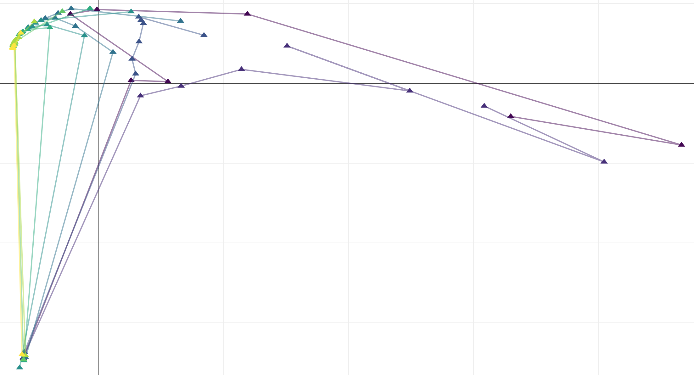
Figure 3: Activation curves. Two-dimensional PCA projections of the activation landscapes from Figure 2 using a larger number of training accuracy thresholds, with consecutive layers connected by line segments (increasing layers generally from left to right) and increasing accuracy thresholds colored from yellow to purple.

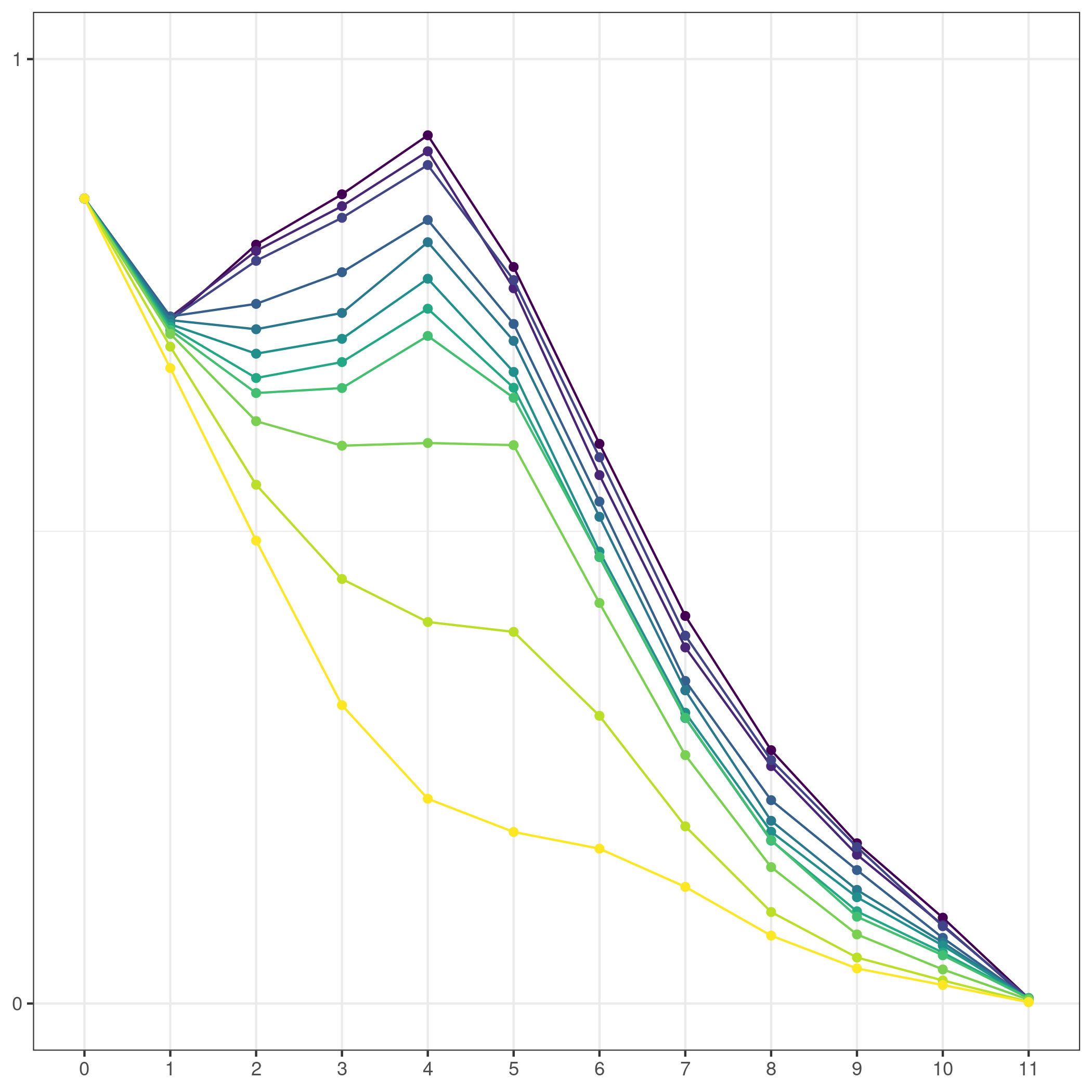
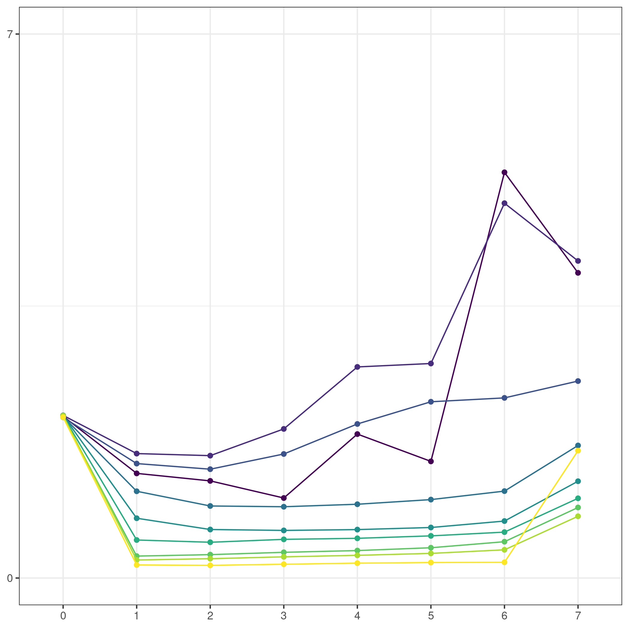
Figure 4: Topological complexity. Average norms of the activation landscapes from Figure 2 using a larger number of training accuracy thresholds with consecutive layers connected by line segments and increasing accuracy thresholds colored from yellow to purple.

TABLE I: The p-values for differences between the activation landscapes in Figure 2 between the various training thresholds. Top: Synthetic data. Bottom: MNIST data.

Training Accuracy	$55\%$	$70\%$	$85\%$	$99.999\%$
$55\%$	$\cdot$	$\cdot$	$\cdot$	$\cdot$
$70\%$	$0.01434$	$\cdot$	$\cdot$	$\cdot$
$85\%$	$0.00000$	$0.00792$	$\cdot$	$\cdot$
$99.999\%$	$0.00000$	$0.00000$	$0.01579$	$\cdot$
Training Accuracy	$60\%$	$80\%$	$95\%$	$99.5\%$
$55\%$	$\cdot$	$\cdot$	$\cdot$	$\cdot$
$70\%$	$0.00000$	$\cdot$	$\cdot$	$\cdot$
$85\%$	$0.00000$	$0.00000$	$\cdot$	$\cdot$
$99.5\%$	$0.00000$	$0.00000$	$0.00000$	$\cdot$

IV Disussion

In Figures 2 and 3 we observe that as the training accuracy threshold increases the activation landscapes are converging toward the expected activation landscape of a fully trained network. Furthermore, the latter seems to accentuate the most significant topological features of the activations. In Figure 4 we plot the norms of these activation landscapes. We make two striking observations. First, the topological complexity of the activations does not decrease monotonically as the data passes through the layers of the well trained networks, contradicting a previous observation on the topology of deep neural networks [30]. Second, as the training threshold increases the topological complexity of the activations tends to increases.

V Conclusion

Our activation landscapes provide a powerful and innovative way for analyzing the evolution of topological information as it passes through the layers of a deep neural network and how this changes throughout the training process. Our method has a number of benefits over previous instances. First, it provides a complete summary of the persistent homology of the activations in each layer in the network. Second, as a feature map and kernel it allows us to easily apply statistics and machine learning in our analysis.

References

- [1] Reza Abbasi-Asl, Yuansi Chen, Adam Bloniarz, Michael Oliver, Ben Willmore, Jack Gallant, and Bin Yu. The DeepTune framework for modeling and characterizing neurons in visual cortex area V4. bioRxiv, page 465534, 2018.
- [2] P. Baldi, P. Sadowski, and D. Whiteson. Enhanced Higgs boson to +- search with deep learning. Physical Review Letters, 114(11):1–6, 2015.
- [3] D. Barnes, Luis Polanco, and Jose A. Perea. A comparative study of machine learning methods for persistence diagrams. Frontiers in Artificial Intelligence, 4, 2021.
- [4] Ulrich Bauer. Ripser: efficient computation of vietoris–rips persistence barcodes. Journal of Applied and Computational Topology, 5(3):391–423, 2021.
- [5] Ulrich Bauer, Michael Kerber, Jan Reininghaus, and Hubert Wagner. Phat – persistent homology algorithms toolbox. In Hoon Hong and Chee Yap, editors, Mathematical Software – ICMS 2014, volume 8592 of Lecture Notes in Computer Science, pages 137–143. Springer Berlin Heidelberg, 2014.
- [6] Paul Bendich, Bei Wang, and Sayan Mukherjee. Local homology transfer and stratification learning. In Proceedings of the Twenty-Third Annual ACM-SIAM Symposium on Discrete Algorithms, pages 1355–1370. ACM, New York, 2012.
- [7] Rickard Bruel Gabrielsson and Gunnar Carlsson. Exposition and interpretation of the topology of neural networks. Proceedings - 18th IEEE International Conference on Machine Learning and Applications, ICMLA 2019, pages 1069–1076, 2019.
- [8] Peter Bubenik. Statistical topological data analysis using persistence landscapes. Journal of Machine Learning Research, 16:77–102, 2015.
- [9] Gunnar Carlsson and Rickard Brüel Gabrielsson. Topological approaches to deep learning. In Nils A. Baas, Gunnar E. Carlsson, Gereon Quick, Markus Szymik, and Marius Thaule, editors, Topological Data Analysis, pages 119–146, Cham, 2020. Springer International Publishing.
- [10] Mathieu Carrière, Frédéric Chazal, Yuichi Ike, Théo Lacombe, Martin Royer, and Yuhei Umeda. Perslay: A neural network layer for persistence diagrams and new graph topological signatures. In Silvia Chiappa and Roberto Calandra, editors, The 23rd International Conference on Artificial Intelligence and Statistics, AISTATS 2020, 26-28 August 2020, Online [Palermo, Sicily, Italy], volume 108 of Proceedings of Machine Learning Research, pages 2786–2796. PMLR, 2020.
- [11] Jeffrey De Fauw, Joseph R. Ledsam, Bernardino Romera-Paredes, Stanislav Nikolov, Nenad Tomasev, Sam Blackwell, Harry Askham, Xavier Glorot, Brendan O’Donoghue, Daniel Visentin, George van den Driessche, Balaji Lakshminarayanan, Clemens Meyer, Faith Mackinder, Simon Bouton, Kareem Ayoub, Reena Chopra, Dominic King, Alan Karthikesalingam, Cían O. Hughes, Rosalind Raine, Julian Hughes, Dawn A. Sim, Catherine Egan, Adnan Tufail, Hugh Montgomery, Demis Hassabis, Geraint Rees, Trevor Back, Peng T. Khaw, Mustafa Suleyman, Julien Cornebise, Pearse A. Keane, and Olaf Ronneberger. Clinically applicable deep learning for diagnosis and referral in retinal disease. Nature Medicine, 24(9):1342–1350, 2018.
- [12] Pietro Di lena, Ken Nagata, and Pierre Baldi. Deep architectures for protein contact map prediction. Bioinformatics, 28(19):2449–2457, 2012.
- [13] Meryll Dindin, Yuhei Umeda, and Frederic Chazal. Topological data analysis for arrhythmia detection through modular neural networks. In Cyril Goutte and Xiaodan Zhu, editors, Advances in Artificial Intelligence, pages 177–188, Cham, 2020. Springer International Publishing.
- [14] Herbert Edelsbrunner, David Letscher, and Afra Zomorodian. Topological persistence and simplification. Discrete Comput. Geom., 28(4):511–533, 2002. Discrete and computational geometry and graph drawing (Columbia, SC, 2001).
- [15] Rickard Brüel Gabrielsson, Bradley J. Nelson, Anjan Dwaraknath, and Primoz Skraba. A topology layer for machine learning. volume 108 of Proceedings of Machine Learning Research, pages 1553–1563, Online, 26–28 Aug 2020. PMLR.
- [16] Ian Goodfellow, Yoshua Bengio, and Aaron Courville. Deep learning. Adaptive Computation and Machine Learning. MIT Press, Cambridge, MA, 2016.
- [17] Alex Graves, Abdel Rahman Mohamed, and Geoffrey Hinton. Speech recognition with deep recurrent neural networks. ICASSP, IEEE International Conference on Acoustics, Speech and Signal Processing - Proceedings, (3):6645–6649, 2013.
- [18] William H. Guss and Ruslan Salakhutdinov. On characterizing the capacity of neural networks using algebraic topology. ArXiv, abs/1802.04443, 2018.
- [19] Awni Y. Hannun, Carl Case, Jared Casper, Bryan Catanzaro, Gregory Frederick Diamos, Erich Elsen, Ryan J. Prenger, Sanjeev Satheesh, Shubho Sengupta, Adam Coates, and A. Ng. Deep speech: Scaling up end-to-end speech recognition. ArXiv, abs/1412.5567, 2014.
- [20] Christoph Hofer, Roland Kwitt, Marc Niethammer, and Andreas Uhl. Deep learning with topological signatures. In I. Guyon, U. V. Luxburg, S. Bengio, H. Wallach, R. Fergus, S. Vishwanathan, and R. Garnett, editors, Advances in Neural Information Processing Systems 30, pages 1634–1644. Curran Associates, Inc., 2017.
- [21] Christoph D. Hofer, Roland Kwitt, Mandar Dixit, and Marc Niethammer. Connectivity-optimized representation learning via persistent homology. 36th International Conference on Machine Learning, ICML 2019, 2019-June:4868–4877, 2019.
- [22] Fred Hohman, Minsuk Kahng, Robert Pienta, and Duen Horng Chau. Visual Analytics in Deep Learning: An Interrogative Survey for the Next Frontiers. IEEE Transactions on Visualization and Computer Graphics, 25(8):2674–2693, 2019.
- [23] Kwangho Kim, Jisu Kim, Manzil Zaheer, Joon Kim, Frederic Chazal, and Larry Wasserman. Pllay: Efficient topological layer based on persistent landscapes. In H. Larochelle, M. Ranzato, R. Hadsell, M. F. Balcan, and H. Lin, editors, Advances in Neural Information Processing Systems, volume 33, pages 15965–15977. Curran Associates, Inc., 2020.
- [24] Diederik P Kingma and Jimmy Ba. Adam: A method for stochastic optimization. arXiv preprint arXiv:1412.6980, 2014.
- [25] Jen-Yu Liu, Shyh-Kang Jeng, and Yi-Hsuan Yang. Applying topological persistence in convolutional neural network for music audio signals. arXiv:1608.07373 [cs.NE], 2016.
- [26] Alessandro Lusci, Gianluca Pollastri, and Pierre Baldi. Deep architectures and deep learning in chemoinformatics: The prediction of aqueous solubility for drug-like molecules. Journal of Chemical Information and Modeling, 53(7):1563–1575, 2013.
- [27] Adam H. Marblestone, Greg Wayne, and Konrad P. Kording. Toward an integration of deep learning and neuroscience. Frontiers in Computational Neuroscience, 10(SEP):1–60, 2016.
- [28] Yuriy Mileyko. Another look at recovering local homology from samples of stratified sets. J. Appl. Comput. Topol., 5(1):55–97, 2021.
- [29] Dimitriy Morozov. Dionysus: a C++ library with various algorithms for computing persistent homology. Software available at http://www.mrzv.org/software/dionysus/, 2012.
- [30] Gregory Naitzat, Andrey Zhitnikov, and Lek-Heng Lim. Topology of deep neural networks. J. Mach. Learn. Res., 21:Paper No. 184, 40, 2020.
- [31] Vidit Nanda. Perseus: the persistent homology software. Software available at http://www.math.rutgers.edu/~vidit/perseus/index.html, 2013.
- [32] Vidit Nanda. Local cohomology and stratification. Found. Comput. Math., 20(2):195–222, 2020.
- [33] Zhenguo Nie, Tong Lin, Haoliang Jiang, and Levent Burak Kara. Topologygan: Topology optimization using generative adversarial networks based on physical fields over the initial domain. ArXiv, abs/2003.04685, 2020.
- [34] Adam Paszke, Sam Gross, Francisco Massa, Adam Lerer, James Bradbury, Gregory Chanan, Trevor Killeen, Zeming Lin, Natalia Gimelshein, Luca Antiga, et al. Pytorch: An imperative style, high-performance deep learning library. Advances in neural information processing systems, 32:8026–8037, 2019.
- [35] Archit Rathore, N. Chalapathi, Sourabh Palande, and Bei Wang. Topoact: Visually exploring the shape of activations in deep learning. Computer Graphics Forum, 40, 2021.
- [36] Bastian Rieck, Matteo Togninalli, Christian Bock, Michael Moor, Max Horn, Thomas Gumbsch, and Karsten Borgwardt. Neural persistence: A complexity measure for deep neural networks using algebraic topology. In International Conference on Learning Representations, 2019.
- [37] Michael Robinson, Christopher Capraro, Cliff Joslyn, Emilie Purvine, Brenda Praggastis, Stephen Ranshous, and Arun V. Sathanur. Local homology of abstract simplicial complexes. ArXiv, abs/1805.11547, 2018.
- [38] Ramprasaath R. Selvaraju, Michael Cogswell, Abhishek Das, Ramakrishna Vedantam, Devi Parikh, and Dhruv Batra. Grad-CAM: Visual Explanations from Deep Networks via Gradient-Based Localization. International Journal of Computer Vision, 128(2):336–359, 2020.
- [39] Gurjeet Singh, Facundo Mémoli, and Gunnar Carlsson. Topological methods for the analysis of high dimensional data sets and 3d object recognition. Eurographics Symposium on Point-Based Graphics, 22, 2007.
- [40] Guillaume Tauzin, Umberto Lupo, Lewis Tunstall, Julian Burella Pérez, Matteo Caorsi, Anibal M. Medina-Mardones, Alberto Dassatti, and Kathryn Hess. giotto-tda: a topological data analysis toolkit for machine learning and data exploration. J. Mach. Learn. Res., 22:Paper No. 39, 6, 2021.
- [41] Yuhei Umeda. Time series classification via topological data analysis. Transactions of the Japanese Society for Artificial Intelligence, 32(3):1–12, 2017.
- [42] Fan Wang, Huidong Liu, Dimitris Samaras, and Chao Chen. Topogan: A topology-aware generative adversarial network. In Andrea Vedaldi, Horst Bischof, Thomas Brox, and Jan-Michael Frahm, editors, Computer Vision – ECCV 2020, pages 118–136, Cham, 2020. Springer International Publishing.
- [43] Satoru Watanabe and Hayato Yamana. Topological measurement of deep neural networks using persistent homology. ArXiv, abs/2106.03016, 2020.
- [44] Jason Yosinski, Jeff Clune, Anh M Nguyen, Thomas J. Fuchs, and Hod Lipson. Understanding neural networks through deep visualization. ArXiv, abs/1506.06579, 2015.
- [45] Dong Yu, Prank Seide, and Gang Li. Conversational speech transcription using context-dependent deep neural networks. Proceedings of the 29th International Conference on Machine Learning, ICML 2012, pages 4–5, 2012.
- [46] Matthew D. Zeiler and Rob Fergus. Visualizing and understanding convolutional networks. Lecture Notes in Computer Science (including subseries Lecture Notes in Artificial Intelligence and Lecture Notes in Bioinformatics), 8689 LNCS(PART 1):818–833, 2014.
- [47] Sharon Zhou, E. Zelikman, Fred Lu, A. Ng, and Stefano Ermon. Evaluating the disentanglement of deep generative models through manifold topology. ArXiv, abs/2006.03680, 2021.
- [48] Afra Zomorodian and Gunnar Carlsson. Computing persistent homology. Discrete Comput. Geom., 33(2):249–274, 2005.