Beyond Exact Gradients: Convergence of Stochastic Soft-Max Policy Gradient Methods with Entropy Regularization

Abstract

Entropy regularization is an efficient technique for encouraging exploration and preventing a premature convergence of (vanilla) policy gradient methods in reinforcement learning (RL). However, the theoretical understanding of entropy regularized RL algorithms has been limited. In this paper, we revisit the classical entropy regularized policy gradient methods with the soft-max policy parametrization, whose convergence has so far only been established assuming access to exact gradient oracles. To go beyond this scenario, we propose the first set of (nearly) unbiased stochastic policy gradient estimators with trajectory-level entropy regularization, with one being an unbiased visitation measure-based estimator and the other one being a nearly unbiased yet more practical trajectory-based estimator. We prove that although the estimators themselves are unbounded in general due to the additional logarithmic policy rewards introduced by the entropy term, the variances are uniformly bounded. We then propose a two-phase stochastic policy gradient (PG) algorithm that uses a large batch size in the first phase to overcome the challenge of the stochastic approximation due to the non-coercive landscape, and uses a small batch size in the second phase by leveraging the curvature information around the optimal policy. We establish a global optimality convergence result and a sample complexity of $\widetilde{\mathcal{O}}(\frac{1}{\epsilon^{2}})$ for the proposed algorithm. Our result is the first global convergence and sample complexity results for the stochastic entropy-regularized vanilla PG method.

68Q32, 68T05, 93E35

1 Introduction

Entropy regularization is a popular technique to encourage exploration and prevent premature convergence for reinforcement learning (RL) algorithms. It was originally proposed in [37] to improve the performance of REINFORCE, a classical family of vanilla policy gradient (PG) methods widely used in practice. Since then, the entropy regularization technique has been applied to a large set of other RL algorithms, including actor-critic [29, 16], Q-learning [31, 15] and trust-region policy optimization methods [40]. It has been shown that the entropy regularization works satisfactorily with deep learning approximations for achieving an impressive empirical performance boost, provides a substantial improvement in exploration and robustness [45, 15, 16], and connects the policy gradient with Q-learning under a one-step entropy regularization [31] or a trajectory-level KL regularization [32].

Recently, there has been considerable interest in the theoretical understanding of how the entropy regularization exploits the geometry of the optimization landscape. In particular, it has been shown in [26, 20, 10] that entropy regularization makes the regularized objective behave similar to a local quadratic function and thus accelerates the convergence of entropy-regularized PG algorithms. In the exact gradient setting, a linear convergence rate has been established for the entropy-regularized PG algorithms with the natural PG (NPG) or policy mirror descent [10, 20] or without the NPG [26]. However, these advantages have mostly been established for the true gradient setting and it is not fully understood whether any geometric property can be exploited to accelerate convergence to global optimality in inexact gradient settings. In the inexact gradient settings,it is proven in [10] that the NPG with the entropy regularization has a sample complexity of $\widetilde{\mathcal{O}}(\frac{1}{\epsilon^{2}})$ where the inexactness of the gradient can be reduced to the inexactness of the state-action value functions. However, the literature on the global optimality convergence and the sample complexity of the most fundamental PG, namely REINFORCE and its variants with regularizations, is still limited, despite its simplicity and popularity in practice. The work [26] has recently developed the first set of global convergence results for PG, which focuses on the soft-max policy parametrization by assuming access to exact PG evaluations. However, their result heavily relies on the access to the exact PG evaluations, and it has been shown that the geometric advantages existing in the exact gradient setting may not be preserved in the stochastic setting [11, 23]. It remains open whether a global optimality convergence result and a low sample complexity can be obtained for the PG with entropy regularization in the practical stochastic gradient setting.

In this paper, we provide an affirmative answer to the above question. In particular, we revisit the classical entropy regularized (vanilla) policy gradient method proposed in the seminal work [37] under the soft-max policy parametrization. We focus on the modern trajectory-level entropy regularization proposed in [15], which is shown to improve over the original one-step entropy regularization adopted in [37, 29] and [31]. Our contributions are summarized below:

• We begin by proposing two new entropy regularized stochastic PG estimators. The first one is an unbiased visitation measure-based estimator, whereas the second one is a nearly unbiased yet more practical trajectory-based estimator. These (nearly) unbiased stochastic PG estimators are the first likelihood-ratio-based estimators in the literature with a trajectory-level entropy regularization. We show that although the estimators themselves are unbounded in general due to the entropy-induced logarithmic policy rewards, the variances indeed remain uniformly bounded.

• One main challenge on extending the result in [26] to the stochastic PG setting is the non-coercive landscape of the entropy-regularized RL. To overcome this challenge, we propose a two-phase stochastic PG algorithm that uses a large batch size in the first phase and uses a small batch size in the second phase. We establish a global optimality convergence result and a sample complexity of $\widetilde{\mathcal{O}}(\frac{1}{\epsilon^{2}})$ for the proposed algorithm under the softmax parameterization. Our result is the first to achieve the sample complexity of $\widetilde{\mathcal{O}}(\frac{1}{\epsilon^{2}})$ for the stochastic entropy-regularized vanilla PG method and matches the sample complexity of the natural PG [10] in terms of dependence on $\epsilon$.

1.1 Related work

Stochastic policy gradient estimators with the original one-step entropy regularization has been proposed and adopted in [37, 29, 31]. For trajectory-level entropy regularization, an exact (visitation measure-based) policy gradient formula has been derived in [2] and later re-derived in the soft-max policy parametrization setting in [26], while stochastic policy gradient estimators have not been formally proposed or studied in the literature. The only exceptions are [32, 16], where [32] provides stochastic policy gradient estimators with a related but different trajectory-level KL regularization term, while [16] utilizes a reparametrization approach to reduce policy stochasticity to a fixed generating distribution. In contrast, we focus on the more widely used trajectory-level entropy regularization and classical likelihood-ratio-based estimators.

The theoretical understanding of policy-based methods has received considerable attention recently [1, 20, 38, 26, 10, 33, 7, 43, 42, 21]. Several techniques have been developed to improve standard PG and achieve a linear convergence rate, such as adding entropy regularization [26, 1, 20, 10], exploiting natural geometries based on Bregman divergences leading to NPG or policy mirror descent [38, 20, 10], and using a geometry-aware normalized PG (GNPG) approach to exploit the non-uniformity of the value function [24]. For the stochastic policy optimization, the existing results have mostly focused on policy mirror ascent methods with the goal of reducing the stochastic analysis to the estimation of the Q-value function [10, 20], as well as incorporating variance reduction techniques to improve the sample complexity of the vanilla PG [22, 13]. The prior literature still lacks globally optimal convergence results and sample complexity for stochastic (vanilla) PG with the entropy regularization.

1.2 Notation

The set of real numbers is shown as $\mathbb{R}$. ${u}\sim\mathcal{U}$ means that $u$ is a random vector sampled from the distribution $\mathcal{U}$. We use $|\mathcal{X}|$ to denote the cardinality of a finite set $\mathcal{X}$. The notions $\mathbb{E}_{\xi}[\cdot]$ and $\mathbb{E}[\cdot]$ refer to the expectation over the random variable $\xi$ and over all of the randomness. The notion $\text{Var}[\cdot]$ refers to the variance. $\Delta(\mathcal{X})$ denotes the probability simplex over a finite set $\mathcal{X}$. For vectors ${x},{y}\in\mathbb{R}^{d}$, let $\|{x}\|_{1}$, $\|{x}\|_{2}$ and $\|{x}\|_{\infty}$ denote the $\ell_{1}$-norm, $\ell_{2}$-norm and $\ell_{\infty}$-norm. We use $\left\langle{x},{y}\right\rangle$ to denote the inner product. For a matrix $A$, the notation $A\succcurlyeq 0$ means that $A$ is positive semi-definite. Given a variable $x$, the notation $a=\mathcal{O}(b(x))$ means that $a\leq C\cdot b(x)$ for some constant $C>0$ that is independent of $x$. Similarly, $a=\widetilde{\mathcal{O}}(b(x))$ indicates that the previous inequality may also depend on the function $\log(x)$, where $C>0$ is again independent of $x$. We use $\text{Geom}(x)$ to denote a geometric distribution with the parameter $x$.

2 Preliminaries

Markov decision processes. RL is generally modeled as a discounted Markov decision process (MDP) defined by a tuple $(\mathcal{S},\mathcal{A},\mathbb{P},r,\gamma)$. Here, $\mathcal{S}$ and $\mathcal{A}$ denote the finite state and action spaces; $\mathbb{P}(s^{\prime}|s,a)$ is the probability that the agent transits from the state $s$ to the state $s^{\prime}$ under the action $a\in\mathcal{A}$; $r(s,a)$ is the reward function, i.e., the agent obtains the reward $r(s_{h},a_{h})$ after it takes the action $a_{h}$ at the state $s_{h}$ at time $h$; $\gamma\in(0,1)$ is the discount factor. Without loss of generality, we assume that $r(s,a)\in[0,\bar{r}]$ for all $s\in\mathcal{S}$ and $a\in\mathcal{A}$. The policy $\pi(a|s)$ at the state $s$ is usually represented by a conditional probability distribution $\pi_{\theta}(a|s)$ associated to the parameter $\theta\in\mathbb{R}^{d}$. Let $\tau=\{s_{0},a_{0},s_{1},a_{1},\ldots\}$ denote the data of a sampled trajectory under policy $\pi_{\theta}$ with the probability distribution over the trajectory as $p(\tau|\theta,\rho)\coloneq\rho(s_{0})\prod_{h=1}^{\infty}\mathbb{P}(s_{h+1}|s_{h},a_{h})\pi_{\theta}(a_{h}|s_{h}),$ where $\rho\in\Delta(\mathcal{S})$ is the probability distribution of the initial state $s_{0}$.

Value functions and Q-functions. Given a policy $\pi$, one can define the state-action value function $Q^{\pi}:\mathcal{S}\times\mathcal{A}\rightarrow\mathbb{R}$ as

$$Q^{\pi}(s,a)\coloneq\mathbb{E}_{\begin{subarray}{c}a_{h}\sim\pi(\cdot|s_{h})\\ s_{h+1}\sim\mathbb{P}(\cdot|s_{h},a_{h})\end{subarray}}\left[\sum_{h=0}^{\infty}\gamma^{h}r(s_{h},a_{h})\bigg{\rvert}s_{0}=s,a_{0}=a\right].$$

The state-value function $V^{\pi}:\mathcal{S}\rightarrow\mathbb{R}$ and the advantage function $A^{\pi}:\mathcal{S}\times\mathcal{A}\rightarrow\mathbb{R}$ can be defined as $V^{\pi}(s)\coloneq\mathbb{E}_{a\sim\pi(\cdot|s)}[Q^{\pi}(s,a)],\ A^{\pi}(s,a)\coloneq Q^{\pi}(s,a)-V^{\pi}(s).$ The goal is to find an optimal policy in the underlying policy class that maximizes the expected discounted return, namely, $\max_{\theta\in\mathbb{R}^{d}}V^{\pi_{\theta}}(\rho)\coloneq\mathbb{E}_{s_{0}\sim\rho}[V^{\pi_{\theta}}(s_{0})].$ For the notional convenience, we will denote $V^{\pi_{\theta}}(\rho)$ by the shorthand notation $V^{\theta}(\rho)$.

Exploratory initial distribution. The discounted state visitation distribution $d_{s_{0}}^{\pi}$ is defined as $d_{s_{0}}^{\pi}(s)\coloneq(1-\gamma)\sum_{h=0}^{\infty}\gamma^{h}\mathbb{P}(s_{h}=s|s_{0},\pi),$ where $\mathbb{P}(s_{h}=s|s_{0},\pi)$ is the state visitation probability that $s_{h}$ is equal to $s$ under the policy $\pi$ starting from the state $s_{0}$. The discounted state visitation distribution under the initial distribution $\rho$ is defined as $d_{\rho}^{\pi}(s)\coloneq\mathbb{E}_{s_{0}\sim\rho}[d_{s_{0}}^{\pi}(s)]$. Furthermore, the state-action visitation distribution induced by $\pi$ and the initial state distribution $\rho$ is defined as $v_{\rho}^{\pi}(s,a)\coloneq d_{\rho}^{\pi}(s)\pi(a|s)$, which can also be written as $v_{\rho}^{\pi}(s,a)\coloneq(1-\gamma)\mathbb{E}_{s_{0}\sim\rho}\sum_{h=0}^{\infty}\gamma^{h}\mathbb{P}(s_{h}=s,a_{h}=a|s_{0},\pi),$ where $\mathbb{P}(s_{h}=s,a_{h}=a|s_{0},\pi)$ is the state-action visitation probability that $s_{h}=s$ and $a_{h}=a$ under $\pi$ starting from the state $s_{0}$. To facilitate the presentation of the main results of the paper, we assume that the state distribution $\rho$ for the performance measure is exploratory [26, 7], i.e., $\rho(\cdot)$ adequately covers the entire state distribution:

Assumption .

The state distribution $\rho$ satisfies $\rho(s)>0$ for all $s\in\mathcal{S}$.

In practice, when the above assumption is not satisfied, we can optimize under another initial distribution $\mu$, i.e., the gradient is taken with respect to the optimization measure $\mu$, where $\mu$ is usually chosen as an exploratory initial distribution that adequately covers the state distribution of some optimal policy. It is shown in [1] that the difficulty of the exploration problem faced by PG algorithms can be captured through the distribution mismatch coefficient defined as $\left\lVert\frac{d_{\rho}^{\pi}}{\mu}\right\rVert_{\infty}$, where $\frac{d_{\rho}^{\pi}}{\mu}$ denotes component-wise division.

Soft-max policy parameterization. In this work, we consider the soft-max parameterization – a widely adopted scheme that naturally ensures that the policy lies in the probability simplex. Specifically, for an unconstrained parameter $\theta\in\mathbb{R}^{|\mathcal{S}||\mathcal{A}|}$, $\pi_{\theta}(a|s)$ is chosen to be $\frac{\exp{(\theta_{s,a})}}{\sum_{a^{\prime}\in\mathcal{A}}\exp{(\theta_{s,a^{\prime}}})}.$ The soft-max parameterization is generally used for MDPs with finite state and action spaces. It is complete in the sense that every stochastic policy can be represented by this class. For the soft-max parameterization, it can be shown that the gradient and Hessian of the function $\log\pi_{\theta}(a|s)$ are bounded, i.e., for all $\theta\in\mathbb{R}^{|\mathcal{S}||\mathcal{A}|}$, $s\in\mathcal{S}$ and $a\in\mathcal{A}$, we have: $\left\lVert\nabla\log\pi_{\theta}(a|s)\right\rVert_{2}\leq 2,\ \left\lVert\nabla^{2}\log\pi_{\theta}(a|s)\right\rVert_{2}\leq 1.$

RL with entropy regularization. Entropy is a commonly used regularization in RL to promote exploration and discourage premature convergence to suboptimal policies [15, 32, 14]. It is far less aggressive in penalizing small probabilities, in comparison to other common regularizations such as log barrier functions [1]. In the entropy-regularized RL (also known as maximum entropy RL), near-deterministic policies are penalized, which is achieved by modifying the value function to

(1) $$V^{\pi}_{\lambda}(\rho)=V^{\pi}(\rho)+\lambda\mathbb{H}(\rho,\pi),$$

where $\lambda\geq 0$ determines the strength of the penalty and $\mathbb{H}(\rho,\pi)$ stands for the discounted entropy defined as $\mathbb{H}(\rho,\pi)\coloneqq\mathbb{E}_{\begin{subarray}{c}s_{0}\sim\rho,a_{t}\sim\pi(\cdot|s_{t})\\ s_{t+1}\sim\mathbb{P}(\cdot|s_{t},a_{t})\end{subarray}}\left[\sum_{t=0}^{\infty}-\gamma^{t}\log\pi(a_{t}|s_{t})\right].$ Equivalently, $V^{\pi}_{\lambda}(\rho)$ can be viewed as the weighted value function of $\pi$ by adjusting the instantaneous reward to be policy-dependent regularized version as $r^{\lambda}(s,a)\coloneqq r(s,a)-\lambda\log\pi(a|s)$, for all $(s,a)\in\mathcal{S}\times\mathcal{A}.$ We also define $V_{\lambda}^{\pi}(s)$ analogously when the initial state is fixed at a given state $s\in\mathcal{S}$. The regularized Q-function $Q_{\lambda}^{\pi}$ of a policy $\pi$, also known as the soft $Q$-function, is related to $V_{\lambda}^{\pi}$ as (for every $s\in\mathcal{S}$ and $a\in\mathcal{A}$)

$$\begin{aligned} Q_{\lambda}^{\pi}(s,a)&=r(s,a)+\gamma\mathbb{E}_{s^{\prime}\sim P(\cdot\mid s,a)}\left[V_{\lambda}^{\pi}\left(s^{\prime}\right)\right],\\ V_{\lambda}^{\pi}(s)&=\mathbb{E}_{a\sim\pi(\cdot\mid s)}\left[-\lambda\log\pi(a\mid s)+Q_{\lambda}^{\pi}(s,a)\right].\end{aligned}$$

Bias due to entropy regularization. Due to the presence of regularization, the optimal solution will be biased with the bias disappearing as $\lambda\rightarrow 0$. More precisely, the optimal policy $\pi^{\ast}_{\lambda}$ of the entropy-regularized problem could also be nearly optimal in terms of the unregularized objective function, as long as the regularization parameter $\lambda$ is chosen to be small. Denote by $\pi^{\ast}$ and $\pi^{\ast}_{\lambda}$ the policies that maximize the objective function and the entropy-regularized objective function with the regularization parameter $\lambda$, respectively. Let $V^{\ast}$ and $V^{\ast}_{\lambda}$ represent the resulting optimal objective value function and the optimal regularized objective value function. [10] shows a simple but crucial connection between $\pi^{\ast}$ and $\pi^{\ast}_{\lambda}$ via the following sandwich bound: $V^{\pi^{\ast}_{\lambda}}(\rho)\leq V^{\pi^{\ast}}(\rho)\leq V^{\pi^{\ast}_{\lambda}}(\rho)+\frac{\lambda\log{|\mathcal{A}|}}{1-\gamma},$ which holds for all initial distribution $\rho$.

3 Stochastic PG methods for entropy regularized RL

3.1 Review: Exact PG methods

The PG method is one of the most popular approaches for a direct policy search in RL [34]. The vanilla PG with exact gradient information and the entropy regularization is summarized in Algorithm 1.

Algorithm 1 Exact PG method

1:  Inputs: $\{\eta_{t}\}_{t=1}^{T}$, $\theta_{1}$.

2:  for $t=1,2,\dots,T-1$ do

3:     $\theta_{t+1}=\theta_{t}+\eta_{t}\nabla V_{\lambda}^{\theta_{t}}(\rho)$.

4:  end for

5:  Outputs: $\theta_{T}$.

The uniform boundedness of the reward function $r$ implies that the absolute value of the entropy-regularized state-value function and Q-value function are bounded.

Lemma 3.1 ([26]).

${V}^{{\theta}}_{\lambda}(s)\leq\frac{\bar{r}+\lambda\log|\mathcal{A}|}{1-\gamma}$ and $Q_{\lambda}^{\pi}(s,a)\leq\frac{\bar{r}+\lambda\log|\mathcal{A}|}{1-\gamma}$ for all $(s,a)\in\mathcal{S}\times\mathcal{A}$ and $\theta\in{\mathbb{R}^{|\mathcal{S}||\mathcal{A}|}}$.

Under the soft-max policy parameterization, one can obtain the following expression for the gradient of $V_{\lambda}^{\pi}(s)$ with respect to the policy parameter $\theta$:

Lemma 3.2 (Proposition 2 in [9]).

The entropy regularized PG with respect to $\theta$ is

(2) $$\nabla V^{\theta}_{\lambda}(\rho)=\frac{1}{1-\gamma}\mathbb{E}_{s,a\sim v_{\rho}^{\pi_{\theta}}}\left[\nabla_{\theta}\log\pi_{\theta}(a|s)\left(Q^{\theta}_{\lambda}(s,a)-\lambda\log\pi_{\theta}(a\mid s)\right)\right],$$

where

$$\frac{\partial}{\partial{\theta_{s^{\prime},a^{\prime}}}}\log\pi_{\theta}(a|s)=\begin{cases}-\pi_{\theta}(a^{\prime}|s^{\prime})\pi_{\theta}(a|s),&(s^{\prime},a^{\prime})\neq(s,a),\\ \pi_{\theta}(a|s)-\pi_{\theta}(a|s)\pi_{\theta}(a|s),&(s^{\prime},a^{\prime})=(s,a).\end{cases}$$

Furthermore, the entropy regularized PG is bounded, i.e., $\left\lVert\nabla V^{\theta}_{\lambda}(\rho)\right\rVert\leq G$ for all $\rho\in\Delta(\mathcal{S})$ and $\theta\in{\mathbb{R}^{|\mathcal{S}||\mathcal{A}|}}$, where $G\coloneq\frac{2(\bar{r}+\lambda\log|\mathcal{A}|)}{(1-\gamma)^{2}}$.

In addition, it is shown that the PG $\nabla V^{\theta}_{\lambda}(\rho)$ is Lipschitz continuous.

Lemma 3.3 (Lemmas 7 and 14 in [26]).

The PG $\nabla V^{\theta}_{\lambda}(\rho)$ is Lipschitz continuous with some constant $L>0$, i.e., $\left\|\nabla V^{\theta_{1}}_{\lambda}(\rho)-\nabla V^{\theta_{2}}_{\lambda}(\rho)\right\|\leq L\cdot\left\|\theta^{1}-\theta^{2}\right\|$, for all $\theta^{1},\theta^{2}\in\mathbb{R}^{d}$, where the value of the Lipschitz constant $L$ is defined as $L:=\frac{8\bar{r}+\lambda(4+8\log{|\mathcal{A}|})}{(1-\gamma)^{3}}$.

Challenges for designing entropy regularized PG estimators. Existing works either consider one-step entropy regularization [36, 29], KL divergence [32], or the re-parametrization technique [15, 16] (which introduces approximation errors that are difficult to quantify exactly). In general, the regularized reward $r-\lambda\log{\pi_{\theta}}$ is policy-dependent and unbounded even though the original reward $r$ is uniformly bounded. Hence, the existing estimators for the un-regularized setting must be modified to account for the policy-dependency and unboundedness while maintaining the essential properties of (nearly) unbiasedness and bounded variances. In the subsequent sections, we propose two (nearly) unbiased estimators and show that although the estimators may be unbounded due to unbounded regularized rewards, the variances are indeed bounded. The proofs of the results in this section can be found in Section 8 of the supplemental materials.

3.2 Sampling the unbiased PG

It results from (2) that in order to obtain an unbiased sample of $\nabla V^{\theta}_{\lambda}(\rho)$, we need to first draw a state-action pair $(s,a)$ from the distribution $\nu_{\rho}^{\pi_{\theta}}(\cdot,\cdot)$ and then obtain an unbiased estimate of the action-value function $Q^{\theta}_{\lambda}(s,a)$. For the standard discounted infinite-horizon RL setting with bounded reward functions, [44] proposes an unbiased estimate of the PG using the random horizon with a geometric distribution and the Monte-Carlo rollouts of finite horizons. However, their result cannot be immediately applied to the entropy-regularized RL setting since the entropy-regularized instantaneous reward $r(s,a)-\lambda\log\pi(a|s)$ could be unbounded when $\pi(a|s)\rightarrow 0$. Fortunately, we can still show that an unbiased PG estimator with the bounded variance for the entropy regularized RL can be obtained in a similar fashion as in [44]. In particular, we will use a random horizon that follows a certain geometric distribution in the sampling process. To ensure that the condition (i) is satisfied, we will use the last sample $\left(s_{H},a_{H}\right)$ of a finite sample trajectory $\left(s_{0},a_{0},s_{1},a_{1},\ldots,s_{H},a_{H}\right)$ to be the sample at which $Q^{\theta}_{\lambda}(\cdot,\cdot)$ is evaluated, where the horizon $H\sim$ $\text{Geom}(1-\gamma)$. It can be shown that $\left(s_{H},a_{H}\right)\sim\nu_{\rho}^{\pi_{\theta}}(s,a).$ Moreover, given $\left(s_{H},a_{H}\right)$, we will perform Monte-Carlo rollouts for another trajectory with the horizon $H^{\prime}\sim\text{Geom}\left(1-\gamma^{1/2}\right)$ independent of $H$, and estimate the advantage function value $Q^{\theta}_{\lambda}(s,a)$ along the trajectory $(s_{0}^{\prime},a_{0}^{\prime},\ldots,s_{H^{\prime}}^{\prime})$ with $s_{0}^{\prime}=s,a_{0}^{\prime}=a$ as follows:

(3) $$\hat{Q}^{{\theta}}_{\lambda}(s,a)= r\left(s_{0}^{\prime},a_{0}^{\prime}\right)+\sum_{t=1}^{H^{\prime}}\gamma^{t/2}\cdot\left(r\left(s_{t}^{\prime},a_{t}^{\prime}\right)-\lambda\log{\pi_{\theta}(a^{\prime}|s^{\prime})}\right).$$

The subroutines of sampling the pair $(s,a)$ from $\nu_{\rho}^{\pi_{\theta}}(\cdot,\cdot)$ and estimating $\hat{Q}^{{\theta}}_{\lambda}(s,a)$ are summarized as Sam-SA and Est-EntQ in Algorithms 4 and 5 in the supplementary material, respectively. Motivated by the form of PG in (2), we propose the following stochastic estimator:

(4) $$\hat{\nabla}V^{\theta}_{\lambda}(\rho)= \frac{1}{1-\gamma}\nabla_{\theta}\log\pi_{\theta}(a_{H}|s_{H})\left(\hat{Q}^{\theta}_{\lambda}(s_{H},a_{H})-\lambda\log\pi_{\theta}(a_{H}\mid s_{H})\right),$$

where $s_{H},a_{H}\leftarrow\textbf{Sam-SA}(\rho,\theta,\gamma)$ and $\hat{Q}^{\theta}_{\lambda}$ is defined in (3). The following lemma shows that the stochastic PG (4) is an unbiased estimator of ${\nabla}V^{\theta}_{\lambda}(\rho)$.

Lemma 3.4.

For $\hat{\nabla}V^{\theta}_{\lambda}(\rho)$ defined in (4), we have $\mathbb{E}[\hat{\nabla}V^{\theta}_{\lambda}(\rho)]={\nabla}V^{\theta}_{\lambda}(\rho).$

The next lemma shows that the proposed PG estimator $\hat{\nabla}V^{\theta}_{\lambda}(\rho)$ has a bounded variance even if it is unbounded when $\pi_{\theta}$ approaches a deterministic policy.

Lemma 3.5.

For $\hat{\nabla}V^{\theta}_{\lambda}(\rho)$ defined in (4), we have $\text{Var}[\hat{\nabla}V^{\theta}_{\lambda}(\rho)]\leq\sigma^{2},$ where $\sigma^{2}=\frac{8}{(1-\gamma)^{2}}\left(\frac{\bar{r}^{2}+(\lambda\log|\mathcal{A}|)^{2}}{(1-\gamma^{1/2})^{2}}\right)$.

3.3 Sampling the trajectory-based PG

Compared to the unbiased PG with a random horizon in (4), a more practical PG estimator is the trajectory-based PG. To derive the trajectory-based PG for the entropy-regularized RL, we first notice that the gradient ${\nabla}V^{\theta}_{\lambda}(\rho)$ can also be written as

(5) $${\nabla}V^{\theta}_{\lambda}(\rho)=\mathbb{E}\left[\left(\sum_{t=0}^{\infty}\nabla\log\pi_{\theta}(a_{t}|s_{t})\right)\left(\sum_{t=0}^{\infty}\gamma^{t}\left(r(s_{t},a_{t})-\lambda\log\pi_{\theta}(a_{t}|s_{t})\right)\right)\right],$$

where the expectation is taken over the trajectory distribution, i.e., $\tau\sim p(\tau|\theta)$.

Since the distribution $p(\tau|\theta)$ is unknown, ${\nabla}V^{\theta}_{\lambda}(\rho)$ needs to be estimated from samples. The trajectory-based estimators include REINFORCE [36], PGT [35] and GPOMDP [3]. In practice, the truncated versions of these trajectory-based PG estimators are used to approximate the infinite sum in the PG estimator. Let $\tau^{H}=\{s_{0},a_{0},s_{1},\ldots,s_{H-1},a_{H-1},s_{H}\}$ denote the truncation of the full trajectory $\tau$ of length $H$. Then, with the commonly used truncated GPOMDP, the truncated PG estimator for ${\nabla}V^{\theta}_{\lambda}$ can be written as:

(6) $$\hat{\nabla}V^{\theta,H}_{\lambda}(\rho)=\sum_{h=0}^{H-1}\left(\sum_{j=0}^{h}\nabla\log\pi_{\theta}(a_{j}|s_{j})\right)\gamma^{h}\left(r(s_{h},a_{h})-\lambda\log\pi_{\theta}(a_{h}|s_{h})\right).$$

Due to the horizon truncation, the PG estimator (6) may no longer be unbiased, but its bias can be very small with a large horizon $H$.

Lemma 3.6.

For $\hat{\nabla}V^{\theta,H}_{\lambda}(\rho)$ defined in (6), we have

$$\left\lVert\mathbb{E}[\hat{\nabla}V^{\theta,H}_{\lambda}(\rho)]-{\nabla}V^{\theta}_{\lambda}(\rho)\right\rVert_{2}\leq\frac{2(\bar{r}+\lambda\log{|\mathcal{A}|})\gamma^{H}}{(1-\gamma)}\left(H+\frac{1}{1-\gamma}\right).$$

From Lemma 3.6, we can observe that the bias is proportional to $\gamma^{H}$ and thus can be controlled to be arbitrarily small with a constant horizon up to some logarithmic term. We then show that the truncated PG estimator $\hat{\nabla}V^{\theta,H}$ has a bounded variance even if it may be unbounded when $\pi_{\theta}$ approaches a deterministic policy.

Lemma 3.7.

For $\hat{\nabla}V^{\theta,H}_{\lambda}(\rho)$ defined in (6), we have

$$\text{Var}(\hat{\nabla}V^{\theta,H}_{\lambda}(\rho))\leq\frac{12\bar{r}^{2}+24\lambda^{2}(\log|\mathcal{A}|)^{2}}{(1-\gamma)^{4}}.$$

3.4 Batched PG algorithms

In practice, we can sample and compute a batch of independently and identically distributed PG estimators $\{\hat{\nabla}V^{\theta,i}_{\lambda}(\rho)\}_{i=1}^{B}$ where $B$ is the batch size, in order to reduce the estimation variance. To maximize the entropy-regularized objective function (1), we can then update the policy parameter $\theta$ by iteratively running gradient-ascent-based algorithms, i.e., $\theta_{t+1}=\theta_{t}+\frac{\eta_{t}}{B}\sum_{i=1}^{B}\hat{\nabla}V^{\theta,i}_{\lambda}(\rho),$ where $\eta_{t}>0$ is the step size. The details of the unbiased PG algorithm with a random horizon for the entropy-regularized RL are provided in Algorithm 2.

Algorithm 2 Ent-RPG: Random-horizon PG for Entropy-regularized RL

1:  Inputs: $\rho,\lambda$, $\theta_{1},B,T,\{\eta_{t}\}_{t=1}^{T}$.

2:  for $t=1,2,\dots,T$ do

3:     for $i=1,2,\dots,B$ do

4:        $s_{H_{t}}^{i},a_{H_{t}}^{i}\leftarrow\textbf{SamSA}(\rho,\theta_{t},\gamma)$.

5:        $\hat{Q}^{\theta_{t},i}_{\lambda}\leftarrow\textbf{Est-EntQ}(s_{H_{t}}^{i},a_{H_{t}}^{i},\theta_{t},\gamma,\lambda)$.

6:     end for

7:     $\theta_{t+1}\leftarrow\theta_{t}+\frac{\eta_{t}}{(1-\gamma)B}\sum_{i=1}^{B}\left[\nabla_{\theta}\log\pi_{\theta_{t}}(a_{H_{t}}^{i}|s_{H_{t}}^{i})\left(\hat{Q}^{\theta_{t},i}_{\lambda}-\lambda\log\pi_{\theta_{t}}(s_{H_{t}}^{i}\mid a_{H_{t}}^{i})\right)\right]$

8:  end for

9:  Outputs: $\theta_{T}$.

Remark 3.8.

For the simplicity of the presentation, we focus on deriving the stochastic PG estimator for the soft-max policy parameterization. However, our results in this section (and also the stationary point convergence result in Section 4.3 below) can be easily extended to the general parameterization $\pi_{\theta}$ as long as $\left\lVert\nabla\log\pi_{\theta}(a|s)\right\rVert_{2}$ and $\left\lVert\nabla^{2}\log\pi_{\theta}(a|s)\right\rVert_{2}$ are bounded for all $(s,a)\in\mathcal{S}\times\mathcal{A}$.

Due to space restrictions and in order to facilitate the presentation of the main ideas, we will mainly focus on the analysis of the unbiased PG estimator in (4) for the rest of the paper. Similar results hold for the trajectory-based PG estimator in (6) since its bias is exponentially small with respect to the horizon (see Lemma 3.6). We leave the formal discussion of these results as future work.

4 Non-coercive landscape

In this section, we first review some key results for the entropy-regularized RL with the exact PG and highlight the difficulty of generalizing these results to the stochastic PG setting, due to the non-coercive landscape.

4.1 Review: Linear convergence with exact PG

A key result from [26] shows that, under the soft-max parameterization, the entropy-regularized value function $V_{\lambda}^{\theta}(\rho)$ in (1) satisfies a non-uniform Łojasiewicz inequality as follows:

Lemma 4.1 (Lemma 15 in [26]).

It holds that $\left\lVert\nabla V_{\lambda}^{\theta}(\rho)\right\rVert_{2}^{2}\geq C(\theta)(V_{\lambda}^{\theta^{\ast}}(\rho)-V_{\lambda}^{\theta}(\rho)),$ where $C(\theta)=\frac{2\lambda}{|\mathcal{S}|}\min_{s}\rho(s)\min_{s,a}\pi_{\theta}(a|s)^{2}\left\lVert\frac{d_{\rho}^{\pi_{\lambda}^{\ast}}}{\rho}\right\rVert_{\infty}^{-1}$.

Furthermore, it is shown in [26] that the action probabilities under the soft-max parameterization are uniformly bounded away from zero if the exact PG is available.

Lemma 4.2 (Lemma 16 in [26]).

Using the exact PG (Algorithm 1) with $\eta_{t}{=\eta}\leq\frac{2}{L}$ for the entropy regularized objective, it holds that $\inf_{t\geq 1}\min_{s,a}\pi_{\theta_{t}}(a|s)>0$.

Remark 4.3.

Note that by Algorithm 1, $\inf_{t\geq 1}\min_{s,a}\pi_{\theta_{t}}(a|s)$ is only dependent on the initialization $\theta_{1}$ and step-size $\eta$ (apart from problem dependent constants). Hence hereafter we denote $c_{\theta_{1},\eta}=\inf_{t\geq 1}\min_{s,a}\pi_{\theta_{t}}(a|s)$.

With Lemmas 3.3, 4.1 and 4.2, it is shown in Theorem 6 of [26] that the convergence rate for the entropy regularized PG is $O\left(e^{-Ct}\right)$, where the value of $C$ depends on $\inf_{t\geq 1}\min_{s,a}\pi_{\theta_{t}}(a|s)>0$ and $\{\theta_{t}\}_{t=1}^{\infty}$ is generated by Algorithm 1. With a bad initialization $\theta_{1}$, $\min_{s,a}\pi_{\theta_{1}}(a|s)$ could be very small and result in a slow convergence rate. When studying the stochastic PG, this issue of bad initialization will create more severe challenges on the convergence, which we will discuss in the following sections.

One main challenge is the boundedness of iterations under the stochastic PG. The iterates of stochastic gradient methods may indeed escape to infinity in general, rendering the entire scheme of stochastic approximation useless [4, 8]. In particular, when using the stochastic truncated PG for the entropy regularized RL, the key result of Lemma 4.2 may no longer hold true. This in turn results in the loss of gradient domination condition in guaranteeing the global convergence.

4.2 Landscape of a simple bandit example

To have a better understanding of the landscape of the entropy-regularized value function, we visualize its landscape in this section. For the simplicity of the visualization, we use a simple bandit example (corresponding to $\gamma=0$) with 2 actions, 2 parameters $(\theta_{1},\theta_{2})$, the reward vector $r=[2,1]$ and the regularization parameter $\lambda=1$. Then, the entropy-regularized value function can be written as $\pi_{\theta}^{\top}\left(r-\log\pi_{\theta}\right)$.

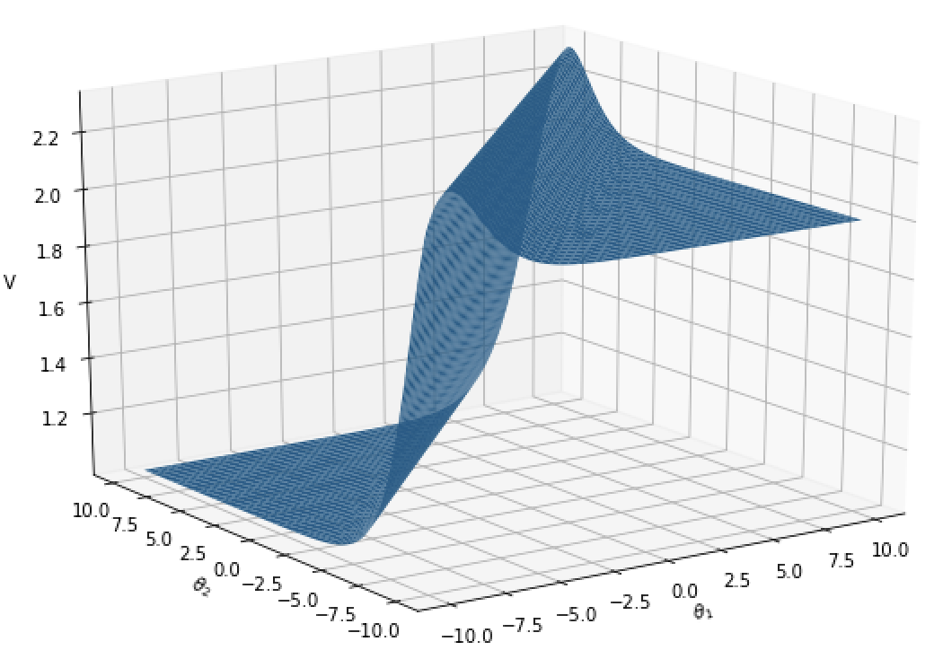
Figure 1: Landscape of $\pi_{\theta}^{\top}\left(r-\log\pi_{\theta}\right)$.

As shown in Figure 1, the entropy-regularized value function is not coercive. When $\theta_{1}$ goes to positive (negative) infinity and $\theta_{2}$ goes to negative (positive) infinity, the landscape will become highly flat. It can also be seen that there is a line space for $(\theta_{1},\theta_{2})$ at which the entropy-regularized value function is maximum.

When the stochastic PG is used, the search direction may be dominated by the gradient estimation noise at the region where the landscape is highly flat. This may further lead to the failure of the globally optimal convergence for the stochastic PG algorithm if the initial point is at the flat region.

4.3 Convergence to the first-order stationary point

Before presenting our main result, we first show that the stochastic PG proposed in Algorithm 2 asymptotically converges to a region where the PG vanishes almost surely if a specific adaptive step-size sequence is used.

Lemma 4.4.

Suppose that the sequence $\{\theta_{t}\}_{t=1}^{\infty}$ is generated by Algorithm 2 for the entropy regularized objective with the step-sizes satisfying $\sum_{t=1}^{\infty}\eta_{t}=\infty,\sum_{t=1}^{\infty}\eta_{t}^{2}<\infty$ and $\eta_{t}\leq\frac{2}{L}$ for all $t=1,2,\ldots$. It holds that $\lim_{t\rightarrow\infty}\left\lVert\nabla V_{\lambda}^{\theta_{t}}(\rho)\right\rVert_{2}=0$ with probability $1$.

This result follows from classic results for the Robbins-Monro algorithm [6, 5, 19] when an unbiased PG estimator with the bounded variance, as in Algorithm 2, is used in the update rule. No requirement on the batch size $B$ is needed in Lemma 4.4. We refer the reader to the supplement in Section 9 for the details of the proof.

However, since the entropy-regularized value function $V_{\lambda}^{\theta}(\rho)$ is not coercive in $\theta$ and it may be the case that the gradient $\nabla V_{\lambda}^{\theta_{t}}(\rho)$ diminishing to $0$ corresponds to $\theta_{t}$ going to infinity instead of converging to a stationary point. In addition, the existing results [4, 5, 19] on the almost surely stationary point convergence rely on the assumption that the trajectories of the process are bounded, i.e., $\sup_{t\geq 0}\left\lVert\theta_{t}\right\rVert<\infty,$ almost surely. This assumption is proven to hold when the function is coercive [27]. However, when the function is not coercive, as in our problem, it is very challenging to characterize the trade-off between the gradient information and the estimation error without additional assumptions.

5 Main result

To overcome the non-coercive landscape challenge, we propose a two-phase stochastic PG algorithm (Algorithm 3). In the first phase, we will use a large batch size to control the estimation error to guarantee that the stochastic PG is informative even in the regime where the landscape is almost flat. After a certain number of iterations, which is a constant with respect to the optimality gap $\epsilon$, the iteration will reach a region where the landscape has enough curvature information. Then, in the second phase, a small batch size is enough to guarantee a fast convergence to the optimal policy.

Before presenting the main result, we first introduce some helpful definitions. Let $D(\theta_{t})=V^{\theta^{\ast}}_{\lambda}(\rho)-V^{\theta_{t}}_{\lambda}(\rho)$ denote the sub-optimality gap. Since the optimal policy of (1) is unique [10], there must exist a continuum of optimal solutions $\Theta^{\ast}\coloneqq\{\theta^{\ast}\in\mathbb{R}^{|\mathcal{S}||\mathcal{A}|}:\frac{\exp(\theta_{s,a}^{\ast})}{\sum_{a^{\prime}}\exp(\theta_{s,a^{\prime}}^{\ast})}=\pi_{\lambda}^{\ast}(a\mid s),\forall s\in\mathcal{S},a\in\mathcal{A}\}$. In addition, we use $\pi_{\theta^{\star}}$ and $\pi_{\lambda}^{\star}$ interchangeably to denote the optimal policy of the entropy-regularized RL. Let $\{\bar{\theta}_{t}\}_{t=1}^{T}$ denote the iterates of the algorithm with the exact PG (Algorithm 1) with $\eta_{t}{=\eta}\leq\frac{1}{2L}$ starting from the initial point ${\theta}_{1}$. For the soft-max parameterization, we have $\theta_{s,a}=\log\pi_{\theta}(a\mid s)+C_{s}$ for all $(s,a)\in\mathcal{S}\times\mathcal{A}$, where $\{C_{s}\}_{s=1}^{|\mathcal{S}|}$ are some constants. Then, we have

$$\min_{\theta^{\ast}\in\Theta^{\ast}}\left\lVert\bar{\theta}_{t}-{\theta}^{\ast}\right\rVert_{2}=\left\lVert\log\pi_{\bar{\theta}_{t}}-\log\pi_{\lambda}^{\ast}\right\rVert_{2},\quad\text{ for all }t=\{1,2,\ldots\}.$$

Furthermore, by Lemma 4.2, we can define $\bar{\Delta}\coloneqq\|\log c_{\bar{\theta}_{1},\eta}-\log\pi_{\lambda}^{\star}\|_{2},$ where $c_{\bar{\theta}_{1},\eta}>0$ is defined in Remark 4.3. Note that $\bar{\Delta}$ is only dependent on $\bar{\theta}_{1}$ and $\eta$ (apart from problem dependent constants), and $\left\lVert\log\pi_{\bar{\theta}_{t}}-\log\pi_{\lambda}^{\ast}\right\rVert_{2}$ $\leq\bar{\Delta}$ for any $\bar{\theta}_{1}$ and $\eta\leq\frac{1}{2L}$. In addition, with a fair degree of hindsight and for some $\delta>0$, we define the stopping time for the iterates $\{\theta_{t}\}_{t=1}^{T}$ as

(7) $$\tau\coloneqq\min\left\{t\Big{|}\min_{\theta^{\ast}\in\Theta^{\ast}}\left\lVert\theta_{t}-\theta^{\ast}\right\rVert_{2}>\left(1+\frac{1}{\delta}\right)\bar{\Delta}\right\},$$

which is the index of the first iterate that exits the bounded region

$$\mathcal{G}^{0}_{\delta}\coloneqq\left\{\theta\in\mathbb{R}^{|\mathcal{S}||\mathcal{A}|}:\min_{\theta^{\ast}\in\Theta^{\ast}}\left\lVert\theta-\theta^{\ast}\right\rVert_{2}\leq\left(1+\frac{1}{\delta}\right)\bar{\Delta}\right\}.$$

Finally, we define $d(\theta_{t})=\min_{\theta^{\ast}\in\Theta^{\ast}}\left\lVert{\theta}_{t}-{\theta}^{\ast}\right\rVert_{2}$. We are now ready to present the main result.

Theorem 5.1.

Consider an arbitrary tolerance level $\delta>0$ and a small enough tolerance level $\epsilon>0$. For every initial point $\theta_{1}$, if $\theta_{T+1}$ is generated by Algorithm 3 with

$$T_{1}\geq\left(\frac{6D(\theta_{1})}{\delta\epsilon_{0}}\right)^{\frac{8L}{C^{0}_{\delta}\ln 2}},\ T_{2}\geq\frac{t_{0}\epsilon_{0}}{6\delta\epsilon}-t_{0},\ T=T_{1}+T_{2},$$

$$B_{1}\geq\max\left\{\frac{30\sigma^{2}}{C^{0}_{\delta}\epsilon_{0}\delta},\frac{6\sigma T_{1}\log{T_{1}}}{\bar{\Delta}L}\right\},\ B_{2}\geq\frac{\sigma^{2}\ln(T_{2}+t_{0})}{6C_{\alpha}\delta\epsilon},$$

$$\eta_{t}=\eta\leq\min\left\{\frac{\log{T_{1}}}{T_{1}L},\frac{8}{C^{0}_{\delta}},\frac{1}{2L}\right\}\ \text{ for }t\leq T_{1},\quad\eta_{t}=\frac{1}{t-T_{1}+t_{0}}\ \text{ for }t>T_{1}$$

where

(8) $$\epsilon_{0}=\min\left\{\left(\frac{\lambda\min_{s}\rho(s)}{6\ln{2}}\right)^{2}\left(\alpha\exp(\frac{-\bar{r}}{(1-\gamma)\lambda})\right)^{4},1\right\},\ t_{0}\geq\sqrt{\frac{3\sigma^{2}}{2\delta\epsilon_{0}}},$$

(9) $$C_{\alpha}\coloneqq\frac{2\lambda}{|\mathcal{S}|}\min_{s}\rho(s)(1-\alpha)^{2}\min_{s,a}\pi_{\theta^{*}}(a|s)^{2}\left\lVert\frac{d_{\rho}^{\pi_{\lambda}^{\ast}}}{\rho}\right\rVert_{\infty}^{-1}>0,$$

(10) $$C^{0}_{\delta}=\frac{2\lambda}{|\mathcal{S}|}\left\lVert\frac{d_{\rho}^{\pi_{\lambda}^{\ast}}}{\rho}\right\rVert_{\infty}^{-1}\min_{s}\rho(s)\min_{\theta\in\mathcal{G}^{0}_{\delta}}\min_{s,a}\pi_{\theta}(a|s)^{2},$$

then we have $\mathbb{P}(D(\theta_{T+1})\leq\epsilon)\geq 1-\delta.$ In total, it requires $\tilde{{\mathcal{O}}}\left(\epsilon^{-2}\right)$ samples to obtain an $\epsilon$-optimal policy with high probability.

Algorithm 3 Two-phase stochastic PG for entropy regularized RL

1:  Inputs: $\rho,\lambda$, $\theta_{1},B_{1},B_{2},T_{1},T,\{\eta_{t}\}_{t=1}^{T}$.

2:  for $t=1,2,\dots,T$ do

3:     if $t\leq T_{1}$ then

4:        $B=B_{1}$

5:     else

6:        $B=B_{2}$

7:     end if

8:     Run lines 3-7 in Algorithm 2

9:  end for

10:  Outputs: $\theta_{T}$;

5.1 Discussion

In Theorem 5.1, we have derived strong last-iterate complexity bounds (in contrast to the predominant running-min and ergodic complexity bounds in the reinforcement learning literature), with the desirable $\widetilde{\mathcal{O}}(1/\epsilon^{2})$ dependency on the targeting tolerance $\epsilon$. That being said, the polynomial dependency on $1/\delta$ and exponential dependencies on other problem- and algorithm-dependent constants also indicate that our bounds may not be tight in general.

The convergence analysis of the stochastic softmax PG with the entropy regularization is challenging due to the weaker regularization effect of the entropy regularization (compared to the log-barrier regularization adopted in previous works on global optimality convergence of policy gradient methods [1, 41]), as well as the “softmax gravity well” induced by the softmax parameterization which has also been observed in the exact gradient setting [26, 25]. In particular, it only entails uniform gradient domination properties for policies that are bounded below uniformly (cf. Lemma 4.1). We thus need to control the trajectory to ensure that $\pi_{\theta_{t}}$ remains in the region where it is uniformly bounded from below for all $t$. However, even with large batches, it is generally difficult to control stochastic trajectories, which eventually leads to the polynomial dependency on $1/\delta$ and the exponential dependencies on some constants. If large batches are not used, then the trajectories would be even harder to control and no guarantees may be attained unless additional structural assumptions are enforced on the underlying MDP .

6 Proof

In this section, we provide the proof of Theorem 5.1. In particular, we will prove that after the first phase of Algorithm 3, the iterates will converge to a neighborhood of the optimal solution with high probability due to the use of a large batch size. Then, we will show how to utilize the curvature information around the optimal policy to guarantee that the action probabilities will still remain uniformly bounded with high probability. Finally, by combining the above two results, we obtain the desirable global convergence and the sample complexity results.

6.1 Global convergence with arbitrary initialization

With a large batch size, we can show that if the iterations with the exact PG are bounded, then the iterations with the unbiased stochastic PG will remain bounded with high probability. This will further imply that the unbiased stochastic PG will converge to the neighborhood of the globally optimal policy with high probability. This is a non-trivial result involving the stopping/hitting time analysis, as presented below.

Lemma 6.1.

Consider arbitrary tolerance levels $\delta>0$ and $\epsilon_{0}>0$. For every initial point $\theta_{1}$, if $\theta_{T}$ is generated by Algorithm 2 with $\eta_{t}=\eta\leq\min\left\{\frac{\log{T_{1}}}{T_{1}L},\frac{8}{C^{0}_{\delta}},\frac{1}{2L}\right\}$, $T_{1}=\left(\frac{6D(\theta_{1})}{\delta\epsilon_{0}}\right)^{\frac{8L}{C^{0}_{\delta}\ln 2}}$, and $B_{1}=\max\left\{\frac{30\sigma^{2}}{C^{0}_{\delta}\epsilon_{0}\delta},\frac{6\sigma}{\bar{\Delta}L}\cdot T_{1}\cdot\log{T_{1}}\right\}$, then we have $\mathbb{P}(D(\theta_{T_{1}})\leq\epsilon_{0})\geq 1-\delta/2.$

To prove Lemma 6.1, we first consider the case when $\tau>T_{1}$, where $\tau$ is defined in (7). Conditioning on this event, we can use Lemma 4.1 to show that $D(\theta_{t})$ is linearly convergent up to some aggregated estimation error.

Lemma 6.2.

If $\eta_{t}{=\eta}\leq\frac{1}{2L}$, then $\mathbb{E}[D(\theta_{T_{1}})\mathbf{1}_{\tau>T_{1}}]\leq\left(1-\frac{\eta C^{0}_{\delta}}{8}\right)^{T_{1}-1}D(\theta_{1})+\frac{5\sigma^{2}}{8C^{0}_{\delta}B_{1}}.$

Proof 6.3.

Let $e_{t}=\nabla V_{\lambda}^{\theta_{t}}(\rho)-u_{t}$, where $u_{t}=\frac{1}{B_{1}}\sum_{i=1}^{B_{1}}\hat{\nabla}V_{\lambda}^{\theta_{t},i}(\rho)$ and $\hat{\nabla}V_{\lambda}^{\theta_{t},i}(\rho)$ is an unbiased estimator of $\nabla V_{\lambda}^{\theta_{t}}(\rho)$. Let $\mathcal{F}_{t}$ denote the sigma field generated by the randomness up to iteration $t$. We define $\mathbb{E}^{t}\coloneqq\mathbb{E}[\cdot|\mathcal{F}_{t}]$ as the expectation operator conditioned on the sigma field $\mathcal{F}_{t}$. Since ${\nabla}V^{\theta}_{\lambda}(\rho)$ is $L$-smooth due to Lemma 3.3, it follows from Lemma 10.1 in the supplementary material:

$$\mathbb{E}^{t}[D(\theta_{t+1})-D(\theta_{t})]\mathbf{1}_{\tau>t}= \mathbb{E}^{t}\left[V_{\lambda}^{\theta_{t}}(\rho)-V_{\lambda}^{\theta_{t+1}}(\rho)\right]\mathbf{1}_{\tau>t}$$

$$\leq \mathbb{E}^{t}\left[-\frac{\eta}{8}\left\lVert u_{t}\right\rVert_{2}^{2}+\frac{3\eta}{4}\left\lVert e_{t}\right\rVert_{2}^{2}\right]\mathbf{1}_{\tau>t}$$

$$\leq \mathbb{E}^{t}\left[-\frac{\eta}{8}\left\lVert u_{t}-\nabla V_{\lambda}^{\theta_{t}}(\rho)+\nabla V_{\lambda}^{\theta_{t}}(\rho)\right\rVert_{2}^{2}+\frac{3\eta}{4}\left\lVert e_{t}\right\rVert_{2}^{2}\right]\mathbf{1}_{\tau>t}$$

$$= \mathbb{E}^{t}\left[-\frac{\eta}{8}\left\lVert\nabla V_{\lambda}^{\theta_{t}}(\rho)\right\rVert_{2}^{2}+\frac{5\eta}{8}\left\lVert e_{t}\right\rVert_{2}^{2}\right]\mathbf{1}_{\tau>t}$$

$$\leq \mathbb{E}^{t}\left[-\frac{\eta C(\theta_{t})}{8}D(\theta_{t})+\frac{5\eta}{8}\left\lVert e_{t}\right\rVert_{2}^{2}\right]\mathbf{1}_{\tau>t},$$

for every $\eta\leq\frac{1}{2L}$, where the second inequality uses the fact that $u_{t}$ is an unbiased estimator of $\nabla V_{\lambda}^{\theta_{t}}(\rho)$ and the last inequality is due to Lemma 4.1. We now consider two cases:

• Case 1: Assume that $\tau>t$, which implies that $\theta_{t}\in\mathcal{G}^{0}_{\delta}$ and $C(\theta_{t})\geq C^{0}_{\delta}$. Then, we have $\mathbb{E}[D(\theta_{t+1})|\mathcal{F}_{t}]\leq\left(1-\frac{\eta C^{0}_{\delta}}{8}\right)D(\theta_{t})+\frac{5\eta}{8}\mathbb{E}\left[\left\lVert e_{t}\right\rVert_{2}^{2}|\mathcal{F}_{t}\right].$

• Case 2: Assume that $\tau\leq t$ which leads to $\mathbb{E}[D(\theta_{t+1})|\mathcal{F}_{t}]\mathbf{1}_{\tau>t}=0$.

Now combining the above two cases yields the inequality

$$\mathbb{E}[D(\theta_{t+1})|\mathcal{F}_{t}]\mathbf{1}_{\tau>t}\leq \left\{(1-\frac{\eta C^{0}_{\delta}}{8})D(\theta_{t})+\frac{5\eta}{8}\mathbb{E}\left[\left\lVert e_{t}\right\rVert_{2}^{2}|\mathcal{F}_{t}\right]\right\}\mathbf{1}_{\tau>t}$$

$$\leq \left(1-\frac{\eta C^{0}_{\delta}}{8}\right)D(\theta_{t})\mathbf{1}_{\tau>t}+\frac{5\eta}{8}\mathbb{E}\left[\left\lVert e_{t}\right\rVert_{2}^{2}|\mathcal{F}_{t}\right].$$

In addition, conditioning on $\mathcal{F}_{t}$ yields that

$$\mathbb{E}[D(\theta_{t+1})\mathbf{1}_{\tau>t+1}|\mathcal{F}_{t}]\leq\mathbb{E}[D(\theta_{t+1})\mathbf{1}_{\tau>t}|\mathcal{F}_{t}]=\mathbb{E}[D(\theta_{t+1})|\mathcal{F}_{t}]\mathbf{1}_{\tau>t},$$

where the last equality uses the fact that $\tau$ is a stopping time and the random variable $\mathbf{1}_{\tau>t}$ is determined completely by the sigma-field $\mathcal{F}_{t}$. Taking the expectations over the sigma-field $\mathcal{F}_{t}$ and then arguing inductively gives rise to

$$\mathbb{E}[D(\theta_{t+1})\mathbf{1}_{\tau>t+1}]\leq \prod_{i=0}^{t}\left(1-\frac{\eta C^{0}_{\delta}}{8}\right)D(\theta_{1})+\sum_{i=0}^{t}\left(1-\frac{\eta C^{0}_{\delta}}{8}\right)^{i}\frac{5\eta}{8}\mathbb{E}\left[\left\lVert e_{i}\right\rVert_{2}^{2}\right]$$

$$\leq \left(1-\frac{\eta C^{0}_{\delta}}{8}\right)^{t}D(\theta_{1})+\frac{5\sigma^{2}}{C^{0}_{\delta}B_{1}}.$$

By setting $t+1=T_{1}$, we obtain that $\mathbb{E}[D(\theta_{T_{1}})\mathbf{1}_{\tau>T_{1}}]\leq\left(1-\frac{\eta C^{0}_{\delta}}{8}\right)^{T_{1}-1}D(\theta_{1})+\frac{5\sigma^{2}}{C^{0}_{\delta}B_{1}}.$ This completes the proof.

We now establish that $\{\theta_{t}\}_{t=1}^{T}$ will be bounded with high probability if the large batch size is used.

Lemma 6.4.

It holds that $\mathbb{P}(\tau\leq T_{1})\leq\frac{\delta\cdot\eta\cdot T_{1}\cdot(1+\eta L)^{T_{1}-1}\cdot{\sigma}}{\bar{\Delta}B_{1}}.$

Proof 6.5.

By the triangle inequality and the fact that the iterations of the algorithm with the exact PG are bounded by $\bar{\Delta}$, we have

$$d(\theta_{t})\leq\left\lVert\theta_{t}-\bar{\theta}_{t}\right\rVert_{2}+\min_{\theta^{\ast}\in\Theta^{\ast}}\left\lVert\theta^{\ast}-\bar{\theta}_{t}\right\rVert_{2}\leq\left\lVert\theta_{t}-\bar{\theta}_{t}\right\rVert_{2}+\bar{\Delta}.$$

Using the update rule of the algorithm with the exact PG $\nabla V_{\lambda}^{\bar{\theta}_{i}}(\rho)$ and the stochastic PG $u_{i}=\frac{1}{B_{1}}\sum_{j=1}^{B_{1}}\hat{\nabla}V_{\lambda}^{\theta_{i},j}(\rho)$, one can write

$$d(\theta_{i})= \left\lVert(\theta_{1}+\sum_{i=1}^{t-1}\eta_{i}u_{i})-(\theta_{1}+\sum_{i=1}^{t-1}\eta_{i}\nabla V_{\lambda}^{\bar{\theta}_{i}}(\rho))\right\rVert_{2}+\bar{\Delta}$$

$$\leq \sum_{i=1}^{t-1}\eta_{i}\left\lVert u_{i}-\nabla V_{\lambda}^{\bar{\theta}_{i}}(\rho)\right\rVert_{2}+\bar{\Delta}$$

$$= \sum_{i=1}^{t-1}\eta_{i}\left\lVert u_{i}-\nabla V_{\lambda}^{{\theta}_{i}}(\rho)+\nabla V_{\lambda}^{{\theta}_{i}}(\rho)-\nabla V_{\lambda}^{\bar{\theta}_{i}}(\rho)\right\rVert_{2}+\bar{\Delta}$$

$$\leq \sum_{i=1}^{t-1}\eta_{i}\left\lVert e_{i}\right\rVert_{2}+\sum_{i=1}^{t-1}\eta_{i}L\left\lVert\theta_{i}-\bar{\theta}_{i}\right\rVert_{2}+\bar{\Delta}.$$

By expanding $\left\lVert\theta_{i}-\bar{\theta}_{i}\right\rVert_{2}$ recursively, it can be concluded that

$$d(\theta_{t})\leq \sum_{i=1}^{t-1}\eta_{i}\left\lVert e_{i}\right\rVert_{2}+\eta_{t-1}L\left\lVert\theta_{t-1}-\bar{\theta}_{t-1}\right\rVert_{2}+\sum_{i=1}^{t-2}\eta_{i}L\left\lVert\theta_{i}-\bar{\theta}_{i}\right\rVert_{2}+\bar{\Delta}$$

$$\leq \sum_{i=1}^{t-1}\eta_{i}\left\lVert e_{i}\right\rVert_{2}+\eta_{t-1}L\sum_{i=1}^{t-2}\eta_{i}\left\lVert e_{i}\right\rVert_{2}+\eta_{t-1}L^{2}\sum_{i=1}^{t-2}\eta_{i}\left\lVert\theta_{i}-\bar{\theta}_{i}\right\rVert_{2}+\sum_{i=1}^{t-2}\eta_{i}L\left\lVert\theta_{i}-\bar{\theta}_{i}\right\rVert_{2}+\bar{\Delta}$$

$$= \sum_{i=1}^{t-1}\eta_{i}\left\lVert e_{i}\right\rVert_{2}+\eta_{t-1}L\sum_{i=1}^{t-2}\eta_{i}\left\lVert e_{i}\right\rVert_{2}+\sum_{i=1}^{t-2}\left(\eta_{i}L+\eta_{t-1}\eta_{i}L^{2}\right)\left\lVert\theta_{i}-\bar{\theta}_{i}\right\rVert_{2}+\bar{\Delta}$$

$$\leq \sum_{i=1}^{t-1}\eta_{i}\left\lVert e_{i}\right\rVert_{2}+\eta_{t-1}L\sum_{i=1}^{t-2}\eta_{i}\left\lVert e_{i}\right\rVert_{2}+\left(\eta_{t-2}L+\eta_{t-1}\eta_{t-2}L^{2}\right)\sum_{i=1}^{t-3}\eta_{i}\left\lVert e_{i}\right\rVert_{2}$$

$$+\sum_{i=1}^{t-3}\left(\left(\eta_{t-2}L+\eta_{t-1}\eta_{t-2}L^{2}\right)\eta_{i}L+\left(\eta_{i}L+\eta_{t-1}\eta_{i}L^{2}\right)\right)\left\lVert\theta_{i}-\bar{\theta}_{i}\right\rVert_{2}+\bar{\Delta}$$

$$\leq \bar{\Delta}+\sum_{i=1}^{t-1}\eta_{i}\left\lVert e_{i}\right\rVert_{2}+\eta_{t-1}L\sum_{i=1}^{t-2}\eta_{i}\left\lVert e_{i}\right\rVert_{2}+\left(\eta_{t-2}L+\eta_{t-1}\eta_{t-2}L^{2}\right)\sum_{i=1}^{t-3}\eta_{i}\left\lVert e_{i}\right\rVert_{2}$$

$$+\sum_{i=1}^{t-4}\left(\left(\eta_{t-2}L+\eta_{t-1}\eta_{t-2}L^{2}\right)\eta_{t-3}L+\left(\eta_{t-3}L+\eta_{t-1}\eta_{t-3}L^{2}\right)\right)\left\lVert e_{i}\right\rVert_{2}$$

$$+\sum_{i=1}^{t-4}\left(\left(\eta_{t-2}\eta_{t-3}L^{2}+\eta_{t-1}\eta_{t-2}\eta_{t-3}L^{3}\right)\eta_{i}L+\left(\eta_{t-3}L+\eta_{t-1}\eta_{t-3}L^{2}\right)\eta_{i}\right)\left\lVert\theta_{i}-\bar{\theta}_{i}\right\rVert_{2}$$

$$= \sum_{i=1}^{t-1}\eta_{i}\prod_{j=i+1}^{t-1}(1+\eta_{j}L)\left\lVert e_{i}\right\rVert_{2}+\bar{\Delta}.$$

Then, by the definition of $\tau$ in (7) and Markov inequality, we obtain

$$\mathbb{P}(\tau\leq T_{1})= \mathbb{P}(\max_{t\in\{1,\ldots,T_{1}\}}d(\theta_{t})\geq(1+\frac{1}{\delta})\bar{\Delta})$$

$$\leq \mathbb{P}(\sum_{i=1}^{T_{1}-1}\eta_{i}\prod_{j=i+1}^{T_{1}-1}(1+\eta_{j}L)\left\lVert e_{i}\right\rVert_{2}+\bar{\Delta}\geq(1+\frac{1}{\delta})\bar{\Delta})$$

$$\leq \frac{\sum_{i=1}^{T_{1}-1}\eta_{i}\prod_{j=i+1}^{T_{1}-1}(1+\eta_{j}L)\mathbb{E}[\left\lVert e_{i}\right\rVert_{2}]}{\frac{1}{\delta}\bar{\Delta}}$$

$$\leq \frac{\delta\eta(1+\eta L)^{T_{1}-1}\sum_{i=1}^{T_{1}-1}\mathbb{E}[\left\lVert e_{i}\right\rVert_{2}]}{\bar{\Delta}},$$

where we use the fact that $\eta_{t}=\eta$ for all $t\in\{1,2,\ldots\}$. Furthermore, since $\mathbb{E}[\left\lVert e_{i}\right\rVert_{2}]\leq\sqrt{\mathbb{E}[\left\lVert e_{i}\right\rVert^{2}_{2}]}\leq\frac{\sigma}{B_{1}}$, we have $\mathbb{P}(\tau\leq T_{1})\leq\frac{\delta\cdot\eta\cdot T_{1}\cdot(1+\eta L)^{T_{1}-1}\cdot{\sigma}}{\bar{\Delta}B_{1}}.$ This completes the proof.

With Lemmas 6.2 and 6.4, we are now ready to prove Lemma 6.1.

Proof 6.6.

By combining Lemmas 6.2 and 6.4, we obtain that

$$\mathbb{P}(D(\theta_{T_{1}})\geq\epsilon_{0})\leq \mathbb{P}({\tau>T_{1}},D(\theta_{T_{1}})\geq\epsilon_{0})+\mathbb{P}({\tau\leq T_{1}},D(\theta_{T_{1}})\geq\epsilon_{0})$$

$$\leq \frac{\mathbb{E}[\mathbf{1}_{\tau>T_{1}}D(\theta_{T_{1}})]}{\epsilon_{0}}+\mathbb{P}({\tau\leq T_{1}})$$

$$\leq \left(1-\frac{\eta C^{0}_{\delta}}{8}\right)^{T_{1}-1}\frac{D(\theta_{1})}{\epsilon_{0}}+\frac{5\sigma^{2}}{C^{0}_{\delta}B_{1}\epsilon_{0}}+\frac{\delta\cdot\eta\cdot T_{1}\cdot(1+\eta L)^{T_{1}-1}\cdot\sigma}{\bar{\Delta}B_{1}}$$

$$\leq \left(1-\frac{\eta C^{0}_{\delta}}{8}\right)^{\frac{8}{\eta C^{0}_{\delta}}\frac{\eta C^{0}_{\delta}T_{1}}{8}}\frac{D(\theta_{1})}{\epsilon_{0}}+\frac{5\sigma^{2}}{C^{0}_{\delta}B_{1}\epsilon_{0}}+\frac{\delta\cdot\eta\cdot T_{1}\cdot(1+\eta L)^{T_{1}-1}\cdot\sigma}{\bar{\Delta}B_{1}}$$

$$\leq \frac{1}{2}^{\frac{\eta C^{0}_{\delta}T_{1}}{8}}\frac{D(\theta_{1})}{\epsilon_{0}}+\frac{5\sigma^{2}}{C^{0}_{\delta}B_{1}\epsilon_{0}}+\frac{\delta\cdot\eta\cdot T_{1}\cdot(1+\eta L)^{T_{1}-1}\cdot\sigma}{\bar{\Delta}B_{1}},$$

where the second inequality holds due to the Markov inequality, and the last inequality holds because of $(1-\frac{1}{m})^{m}\leq\frac{1}{2}$ for all $m\geq 1$ and $\frac{8}{\eta C^{0}_{\delta}}\geq 1$. By taking $\eta\leq\min\left\{\frac{\log{T_{1}}}{T_{1}L},\frac{8}{C^{0}_{\delta}},\frac{1}{2L}\right\}$, we obtain

$$\mathbb{P}(D(\theta_{T_{1}})\geq\epsilon_{0})\leq \frac{1}{2}^{\frac{C^{0}_{\delta}\log{T_{1}}}{8L}}\frac{D(\theta_{1})}{\epsilon_{0}}+\frac{5\sigma^{2}}{C^{0}_{\delta}B_{1}\epsilon_{0}}+\frac{\delta\cdot\log{T_{1}}\cdot(1+\frac{\log{T_{1}}}{T_{1}})^{T_{1}-1}\cdot{\sigma}}{\bar{\Delta}B_{1}L}$$

$$\leq \frac{1}{2}^{\frac{C^{0}_{\delta}\log{T_{1}}}{8L}}\frac{D(\theta_{1})}{\epsilon_{0}}+\frac{5\sigma^{2}}{C^{0}_{\delta}B_{1}\epsilon_{0}}+\frac{\delta\cdot\log{T_{1}}\cdot(1+\frac{\log{T_{1}}}{T_{1}})^{\frac{T_{1}}{\log{T_{1}}}\cdot\log{T_{1}}}\cdot{\sigma}}{\bar{\Delta}B_{1}L}$$

$$\leq \frac{1}{2}^{\frac{C^{0}_{\delta}\log{T_{1}}}{8L}}\frac{D(\theta_{1})}{\epsilon_{0}}+\frac{5\sigma^{2}}{C^{0}_{\delta}B_{1}\epsilon_{0}}+\frac{\delta\cdot\log{T_{1}}\cdot T_{1}\cdot{\sigma}}{\bar{\Delta}B_{1}L}$$

$$\leq \frac{1}{T_{1}^{\frac{\ln{2}C^{0}_{\delta}}{8L}}}\frac{D(\theta_{1})}{\epsilon_{0}}+\frac{5\sigma^{2}}{C^{0}_{\delta}B_{1}\epsilon_{0}}+\frac{\delta\cdot\log{T_{1}}\cdot T_{1}\cdot{\sigma}}{\bar{\Delta}B_{1}L},$$

where we have used $(1+x)^{1/x}\leq e$ in the third inequality and $a^{\ln{b}}=b^{\ln{a}}$ in the last inequality. To guarantee $\mathbb{P}(D(\theta_{T_{1}})\geq\epsilon_{0})\leq\delta/2$, it suffices to have

$$T_{1}=\left(\frac{6D(\theta_{1})}{\delta\epsilon_{0}}\right)^{\frac{8L}{C^{0}_{\delta}\ln 2}}\ \text{ and }\ B_{1}=\max\left\{\frac{30\sigma^{2}}{C^{0}_{\delta}\epsilon_{0}\delta},\frac{6\sigma}{\bar{\Delta}L}\cdot T_{1}\cdot\log{T_{1}}\right\}.$$

This completes the proof.

6.2 Uniformly bounded action probabilities given a good initialization

Lemma 6.7.

Given a tolerance level $\delta>0$, let $\pi_{\lambda}^{*}$ be the optimal policy of $V_{\lambda}^{\theta}(\rho)$. Assume further that Algorithm 2 is run for $T_{2}$ iterates with a step-size sequence of the form $\eta_{t}=1/(t+t_{0})$ and a batch-size sequence $B\geq\frac{1}{\eta_{t}}$ for all $t=1,2,\ldots,T_{2}$. If $t_{0}\geq\sqrt{\frac{3\sigma^{2}}{2\delta\epsilon_{0}}}$, and $\pi_{\theta_{1}}$ is initialized in a neighborhood $\mathcal{U}_{1}$ such that

(11) $$\mathcal{U}_{1}=\left\{\pi\in\Delta(\mathcal{A})^{|\mathcal{S}|}:D(\pi)\leq\epsilon_{0}\right\},$$

where $\epsilon_{0}=\min\left\{\left(\frac{\lambda\min_{s}\rho(s)}{6\ln{2}}\right)^{2}\left(\alpha\exp(\frac{-\bar{r}}{(1-\gamma)\lambda})\right)^{4},1\right\}$ and the constant $\alpha\in(0,1)$, then the event

(12) $$\Omega_{\alpha,1}^{T_{2}}=\left\{\min_{s,a}\pi_{\theta_{t}}(a|s)\geq(1-\alpha)\min_{s,a}\pi_{\lambda}^{*}(a|s),\text{ for all }t=1,2,\ldots,T_{2}\right.\Big{\}}$$

occurs with probability at least $1-\delta/6$.

To prove Lemma 6.7, we first characterize the maximum amount by which $D(\theta_{t})$ can grow at each step.

Lemma 6.8.

Suppose that $\{\theta_{t}\}$ is generated by Algorithm 2 with $0<\eta_{t}\leq\frac{(1-\gamma)^{3}}{16\bar{r}+\lambda(8+16\log|\mathcal{A}|)}$ for all $t\geq 1$. We have

(13) $$D(\theta_{t+1})\leq \left(1-\frac{\eta_{t}C(\theta_{t})}{4}\right)D(\theta_{t})-\frac{\eta_{t}}{2}\xi_{t}+\frac{\eta_{t}}{4}\left\lVert e_{t}\right\rVert_{2}^{2},$$

where $\xi_{t}=\langle e_{t},{\nabla}V^{\theta_{t}}_{\lambda}(\rho)\rangle$ and $e_{t}=\hat{\nabla}V_{\lambda}^{\theta_{t}}(\rho)-{\nabla}V_{\lambda}^{\theta_{t}}(\rho)$.

Proof 6.9.

Since ${\nabla}V^{\theta}_{\lambda}(\rho)$ is $L$-smooth in light of Lemma 3.3, it follows from Lemma 10.1 that

$$D(\theta_{t+1})-D(\theta_{t})\leq -\frac{\eta_{t}}{4}\left\lVert\hat{\nabla}V^{\theta}_{\lambda}(\rho)\right\rVert_{2}^{2}+\frac{\eta_{t}}{2}\left\lVert e_{t}\right\rVert_{2}^{2}$$

$$\leq -\frac{\eta_{t}}{4}\left\lVert\hat{\nabla}V^{\theta_{t}}_{\lambda}(\rho)-{\nabla}V^{\theta_{t}}_{\lambda}(\rho)+{\nabla}V^{\theta_{t}}_{\lambda}(\rho)\right\rVert_{2}^{2}+\frac{\eta_{t}}{2}\left\lVert e_{t}\right\rVert_{2}^{2}$$

$$= -\frac{\eta_{t}}{4}\left\lVert\hat{\nabla}V^{\theta_{t}}_{\lambda}(\rho)-{\nabla}V^{\theta_{t}}_{\lambda}(\rho)\right\rVert_{2}^{2}-\frac{\eta_{t}}{4}\left\lVert\hat{\nabla}V^{\theta_{t}}_{\lambda}(\rho)\right\rVert_{2}^{2}$$

$$-\frac{\eta_{t}}{2}\langle e_{t},{\nabla}V^{\theta_{t}}_{\lambda}(\rho)\rangle+\frac{\eta_{t}}{2}\left\lVert e_{t}\right\rVert_{2}^{2}$$

$$= -\frac{\eta_{t}}{4}\left\lVert{\nabla}V^{\theta_{t}}_{\lambda}(\rho)\right\rVert_{2}^{2}-\frac{\eta_{t}}{2}\langle e_{t},{\nabla}V^{\theta_{t}}_{\lambda}(\rho)\rangle+\frac{\eta_{t}}{4}\left\lVert e_{t}\right\rVert_{2}^{2}$$

$$\leq -\frac{\eta_{t}C(\theta_{t})}{4}D(\theta_{t})-\frac{\eta_{t}}{2}\langle e_{t},{\nabla}V^{\theta_{t}}_{\lambda}(\rho)\rangle+\frac{\eta_{t}}{4}\left\lVert e_{t}\right\rVert_{2}^{2},$$

for every $\eta_{t}\leq\frac{1}{2L}$, where the last inequality is due to Lemma 4.1.

The quantity by which $D(\theta_{t})$ can grow at each step can be large for any given $t$ but we will show that, with high probability, the aggregation of these errors remains controllably small under the stated conditions on the step-sizes and batch size.

Similar as the techniques used in [17, 18, 24, 28, 27], we now encode the error terms in (13) as $M_{n}=\sum_{t=1}^{n}\eta_{t}\xi_{t}$ and $S_{n}=\sum_{t=1}^{n}\frac{\eta_{t}}{4}\left\lVert e_{t}\right\rVert_{2}^{2}.$ Since $\mathbb{E}\left[\xi_{n}\right]=0$, we have $\mathbb{E}\left[M_{n}\right]=M_{n-1}$. Therefore, $M_{n}$ is a zero-mean martingale; likewise, $\mathbb{E}\left[S_{n}\right]\geq S_{n-1}$, and therefore $S_{n}$ is a submartingale. The difficulty of controlling the errors in $M_{n}$ and $S_{n}$ lies in the fact that the estimation error $e_{n}$ may be unbounded. Because of this, we need to take a less direct, step-by-step approach to bound the total error increments conditioned on the event that $D(\theta_{n})$ remains close to $D(\theta^{\ast})$. We begin by introducing the “cumulative mean square error” $R_{n}=M_{n}^{2}+S_{n}.$ By construction, we have

$$R_{n} =\left(M_{n-1}+\eta_{n}\xi_{n}\right)^{2}+S_{n-1}+\frac{1}{4}\eta_{n}\left\|e_{n}\right\|^{2}=R_{n-1}+2M_{n-1}\eta_{n}\xi_{n}+\eta_{n}^{2}\xi_{n}^{2}+\frac{1}{4}\eta_{n}\left\|e_{n}\right\|^{2}.$$

Hence, $\mathbb{E}\left[R_{n}\right]=R_{n-1}+2M_{n-1}\eta_{n}\mathbb{E}\left[\xi_{n}\right]+\eta_{n}^{2}\mathbb{E}\left[\xi_{n}^{2}\right]+\frac{1}{4}\eta_{n}\mathbb{E}\left[\left\|e_{n}\right\|^{2}\right]\geq R_{n-1},$ i.e., $R_{n}$ is a submartingale. With a fair degree of hindsight, we define $\mathcal{U}$ as:

(14) $$\mathcal{U}=\left\{\pi\in\Delta(\mathcal{A})^{|\mathcal{S}|}:D(\pi)\leq 2\epsilon_{0}+\sqrt{\epsilon_{0}}\right\}.$$

To condition it further, we also define the events

$$\Omega_{n}\equiv\Omega_{n}(\epsilon_{0})=\left\{\pi_{\theta_{t}}\in\mathcal{U}\text{ for all }t=1,2,\ldots,n\right\}$$

$$E_{n}\equiv E_{n}(\epsilon_{0})=\left\{R_{t}\leq\epsilon_{0}\text{ for all }t=1,2,\ldots,n\right\}$$

By definition, we also have $\Omega_{0}=E_{0}=\Omega$ (because the set-building index set for $k$ is empty in this case, and every statement is true for the elements of the empty set). These events will play a crucial role in the sequel as indicators of whether $\pi_{\theta_{t}}$ has escaped the vicinity of $\pi_{\lambda}^{\star}$.

Let the notation $\mathbb{1}_{A}$ indicate the logical indicator of an event $A\subseteq\Omega$, i.e., $\mathbb{1}_{A}(\omega)=1$ if $\omega\in A$ and $\mathbb{1}_{A}(\omega)=0$ otherwise. For brevity, we write $\mathcal{F}_{n}=\sigma(\theta_{1},\ldots,\theta_{n})$ for the natural filtration of $\theta_{n}$. Now, we are ready to state the next lemma.

Lemma 6.10.

Let $\pi_{\lambda}^{*}$ be the optimal policy. Then, for all $n\in\{1,2,\ldots\}$, the following statements hold:

1. $\Omega_{n+1}\subseteq\Omega_{n}$ and $E_{n+1}\subseteq E_{n}$.

2. $E_{n-1}\subseteq\Omega_{n}$.

3. Consider the “large noise” event

   $$\tilde{E}_{n} \equiv E_{n-1}\backslash E_{n}=E_{n-1}\cap\left\{R_{n}>\epsilon_{0}\right\}$$

   $$=\left\{R_{t}\leq\epsilon_{0}\text{ for all }t=1,2,\ldots,n-1\text{ and }R_{n}>\epsilon_{0}\right\}$$

   and let $\tilde{R}_{n}=R_{n}\mathbb{1}_{E_{n-1}}$ denote the cumulative error subject to the noise being “small” until time $n$. Then,

   (15) $$\mathbb{E}\left[\tilde{R}_{n}\right]\leq\mathbb{E}\left[\tilde{R}_{n-1}\right]+G^{2}\sigma^{2}\eta_{n}^{2}+\frac{\eta_{n}\sigma^{2}}{4B}-\epsilon_{0}\mathbb{P}\left(\tilde{E}_{n-1}\right).$$

   By convention, we write $\tilde{E}_{0}=\varnothing$ and $\tilde{R}_{0}=0$.

Proof 6.11.

Statement 1 is obviously true. For Statement 2, we proceed inductively:

• For the base case $n=1$, we have $\Omega_{1}=\left\{\pi_{\theta_{1}}\in\mathcal{U}\right\}\supseteq\left\{\pi_{\theta_{1}}\in\mathcal{U}_{1}\right\}=\Omega$ because $\pi_{\theta_{1}}$ is initialized in $\mathcal{U}_{1}\subseteq\mathcal{U}$. Since $E_{0}=\Omega$, our claim follows.

• For the inductive step, assume that $E_{n-1}\subseteq\Omega_{n}$ for some $n\geq 1$. To show that $E_{n}\subseteq\Omega_{n+1}$, we fix a realization in $E_{n}$ such that $R_{t}\leq\varepsilon$ for all $t=1,2,\ldots,n$. Since $E_{n}\subseteq E_{n-1}$, the inductive hypothesis posits that $\Omega_{n}$ also occurs, i.e., $\pi_{\theta_{t}}\in\mathcal{U}$ for all $t=1,2,\ldots,n$; hence, it suffices to show that $\pi_{\theta_{n+1}}\in\mathcal{U}$. To that end, given that $\pi_{\theta_{t}}\in{\mathcal{U}}$ for all $t=1,2,\ldots n$, the distance estimate (13) readily gives $D(\theta_{t+1})\leq D(\theta_{t})+\eta_{t}\xi_{t}+\frac{\eta_{t}}{4}\left\lVert e_{t}\right\rVert_{2}^{2}$ for all $t=1,2,\ldots,n.$ Therefore, after telescoping, we obtain

  $$D(\theta_{n+1})\leq D(\theta_{1})+M_{n}+S_{n}\leq D(\theta_{1})+\sqrt{R_{n}}+R_{n}\leq\varepsilon+\sqrt{\varepsilon}+\varepsilon=2\varepsilon+\sqrt{\varepsilon}$$

  by the inductive hypothesis. This completes the induction.

For Statement 3, we decompose $\tilde{R}_{n}$ as

$$\tilde{R}_{n}=R_{n}\mathbb{1}_{E_{n-1}} =R_{n-1}\mathbb{1}_{E_{n-1}}+\left(R_{n}-R_{n-1}\right)\mathbb{1}_{E_{n-1}}$$

$$=R_{n-1}\mathbb{1}_{E_{n-2}}-R_{n-1}\mathbb{1}_{\tilde{E}_{n-1}}+\left(R_{n}-R_{n-1}\right)\mathbb{1}_{E_{n-1}}$$

$$=\tilde{R}_{n-1}+\left(R_{n}-R_{n-1}\right)\mathbb{1}_{E_{n-1}}-R_{n-1}\mathbb{1}_{\tilde{E}_{n-1}}$$

where we have used the fact that $E_{n-1}=E_{n-2}\backslash\tilde{E}_{n-1}$ so $\mathbb{1}_{E_{n-1}}=\mathbb{1}_{E_{n-2}}-\mathbb{1}_{\tilde{E}_{n-1}}$ (recall that $\left.E_{n-1}\subseteq E_{n-2}\right)$. Then, by the definition of $R_{n}$, we have

$$R_{n}-R_{n-1}=2M_{n-1}\eta_{n}\xi_{n}+\eta_{n}^{2}\xi_{n}^{2}+\frac{1}{4}\eta_{n}\left\|e_{n}\right\|^{2}$$

and therefore

(16) $$\mathbb{E}\left[\left(R_{n}-R_{n-1}\right)\mathbb{1}_{E_{n-1}}\right] =2\eta_{n}\mathbb{E}\left[M_{n-1}\xi_{n}\mathbb{1}_{E_{n-1}}\right]+\eta_{n}^{2}\mathbb{E}\left[\xi_{n}^{2}\mathbb{1}_{E_{n-1}}\right]+\frac{1}{4}\eta_{n}\mathbb{E}\left[\left\|e_{n}\right\|^{2}\mathbb{1}_{E_{n-1}}\right].$$

However, since $E_{n-1}$ and $M_{n-1}$ are both $\mathcal{F}_{n}$-measurable, we have the following estimates:

• For the term in (16), by the unbiasedness of the gradient estimator shown in Lemma 3.4, we have: $\mathbb{E}\left[M_{n-1}\xi_{n}\mathbb{1}_{E_{n-1}}\right]=\mathbb{E}\left[M_{n-1}\mathbb{1}_{E_{n-1}}\mathbb{E}\left[\xi_{n}\mid\mathcal{F}_{n}\right]\right]=0.$

• The second term in (16) is where the conditioning on $E_{n-1}$ plays the most important role. It holds that:

  $$\mathbb{E}\left[\xi_{n}^{2}\mathbb{1}_{E_{n-1}}\right] =\mathbb{E}\left[\mathbb{1}_{E_{n-1}}\mathbb{E}\left[\left\langle e_{n},\nabla V_{\lambda}^{\theta_{n}}(\rho)\right\rangle^{2}\mid\mathcal{F}_{n}\right]\right]$$

  $$\leq\mathbb{E}\left[\mathbb{1}_{E_{n-1}}\left\|\nabla V_{\lambda}^{\theta_{n}}(\rho)\right\|^{2}\mathbb{E}\left[\left\|e_{n}\right\|^{2}\mid\mathcal{F}_{n}\right]\right]$$

  $$\leq\mathbb{E}\left[\mathbb{1}_{\Omega_{n}}\left\|\nabla V_{\lambda}^{\theta_{n}}(\rho)\right\|^{2}\mathbb{E}\left[\left\|e_{n}\right\|^{2}\mid\mathcal{F}_{n}\right]\right]$$

  $$\leq G^{2}\sigma^{2}$$

  where the first inequality is due to the Cauchy-Schwarz inequality, the second inequality follows from $E_{n-1}\subseteq\Omega_{n}$ and the last inequality results from Lemmas 3.2 and 3.5.

• Finally, for the third term in (16), we have:

  (17) $$\frac{\eta_{n}}{4}\mathbb{E}\left[\left\lVert e_{n}\right\rVert_{2}^{2}\mathbb{1}_{E_{n-1}}\right]\leq\frac{\eta_{n}\sigma^{2}}{4B}.$$

Thus, putting together all of the above, we obtain $\mathbb{E}\left[\left(R_{n}-R_{n-1}\right)\mathbb{1}_{E_{n-1}}\right]\leq G^{2}\sigma^{2}\eta_{n}^{2}$ $+\frac{\eta_{n}\sigma^{2}}{4B}.$ Since $R_{n-1}>\varepsilon$ if $\tilde{E}_{n-1}$ occurs, we obtain $\mathbb{E}\left[R_{n-1}\mathbb{1}_{\tilde{E}_{n-1}}\right]\geq\varepsilon\mathbb{E}\left[\mathbb{1}_{\tilde{E}_{n-1}}\right]=\varepsilon\mathbb{P}\left(\tilde{E}_{n-1}\right).$ This completes the proof of Statement 3.

With the above results, we can show that the cumulative mean square error $R_{n}$ is small with high probability at all times.

Lemma 6.12.

Consider an arbitrary tolerance level $\delta>0$. If Algorithm 2 is run with a step-size schedule of the form $\eta_{t}=1/(t+t_{0})$ where $t_{0}\geq\sqrt{\frac{3\sigma^{2}}{2\delta\epsilon_{0}}}$ and a batch size schedule $B_{t}\geq\frac{1}{\eta_{t}}$, we have $\mathbb{P}\left(E_{n}\right)\geq 1-\delta/6,\text{ for all }n=1,2,\ldots$

Proof 6.13.

We begin by bounding the probability of the “large noise” event $\tilde{E}_{n}=E_{n-1}\backslash E_{n}$ as follows:

$$\mathbb{P}\left(\tilde{E}_{n}\right) =\mathbb{P}\left(E_{n-1}\backslash E_{n}\right)=\mathbb{P}\left(E_{n-1}\cap\left\{R_{n}>\varepsilon\right\}\right)=\mathbb{E}\left[\mathbb{1}_{E_{n-1}}\times\mathbb{1}_{\left\{R_{n}>\varepsilon\right\}}\right]$$

$$\leq\mathbb{E}\left[\mathbb{1}_{E_{n-1}}\times\left(R_{n}/\varepsilon\right)\right]=\mathbb{E}\left[\tilde{R}_{n}\right]/\varepsilon,$$

which is derived by using the fact that $R_{n}\geq 0$ (so $\left.\mathbb{1}_{\left\{R_{n}>\varepsilon\right\}}\leq R_{n}/\varepsilon\right)$. Now, by summing up (15), we conclude that $\mathbb{E}\left[\tilde{R}_{n}\right]\leq\mathbb{E}\left[\tilde{R}_{0}\right]+\frac{\sigma^{2}}{4B}\sum_{t=1}^{n}\eta_{t}-\varepsilon\sum_{t=1}^{n}\mathbb{P}\left(\tilde{E}_{t-1}\right).$ Hence, combining the above results, we obtain the estimate

$$\sum_{t=1}^{n}\mathbb{P}\left(\tilde{E}_{k}\right)\leq\frac{\sigma^{2}}{4B\epsilon_{0}}\sum_{t=1}^{n}\eta_{t}\leq\frac{\sigma^{2}}{4\epsilon_{0}}\sum_{t=1}^{n}\eta_{t}^{2}\leq\frac{\sigma^{2}\Gamma}{4\epsilon_{0}},$$

where $\Gamma=\sum_{t=1}^{\infty}\eta_{t}^{2}=\sum_{t=1}^{\infty}(t+t_{0})^{-2}$, and we have used the relations that $\tilde{R}_{0}=0$ and $\tilde{E}_{0}=\varnothing$ (by convention). By choosing $t_{0}\geq\sqrt{\frac{3\sigma^{2}}{2\delta\epsilon_{0}}}$, we ensure that $\frac{\sigma^{2}\Gamma}{4\epsilon_{0}}<\delta/6$; moreover, since the events $\tilde{E}_{t}$ are disjoint for all $t=1,2,\ldots$, we obtain $\mathbb{P}\left(\bigcup_{t=1}^{n}\tilde{E}_{t}\right)=\sum_{t=1}^{n}\mathbb{P}\left(\tilde{E}_{t}\right)\leq\delta/6.$ Hence, $\mathbb{P}\left(E_{n}\right)=\mathbb{P}\left(\bigcap_{t=1}^{n}\tilde{E}_{t}^{\mathrm{c}}\right)\geq 1-\delta/6$ as claimed.

We are now ready to prove Lemma 6.7.

Proof 6.14.

Since the sequence $\Omega_{n}$ is decreasing and $\Omega_{n}\supseteq E_{n-1}$ (by the second part of Lemma 6.10), Lemma 6.12 yields that $\mathbb{P}\left(\Omega_{T_{2}}\right)\geq\inf_{n}\mathbb{P}\left(\Omega_{n}\right)\geq\inf_{n}\mathbb{P}\left(E_{n-1}\right)\geq 1-\delta/6$ provided that $t_{0}$ is chosen large enough.

Now, it remains to show that $\Omega_{T_{2}}\subseteq\Omega_{\alpha,1}^{T_{2}}$. We fix a realization in $\Omega_{T_{2}}$ such that $D(\theta_{t})\leq 2\epsilon_{0}+\sqrt{\epsilon_{0}}$ for all $t=1,2,\ldots,T_{2}$. By Lemma 11.1, we have

$$\left|\pi_{\theta_{t}}({a}\mid{s})-\pi_{{\theta^{*}}}({a}\mid{s})\right|\leq\sqrt{\frac{2D({\theta_{t}})\ln 2}{\lambda\min_{s}\rho(s)}}\leq\sqrt{\frac{2(2\epsilon_{0}+\sqrt{\epsilon_{0}})\ln 2}{\lambda\min_{s}\rho(s)}}$$

$$\leq\sqrt{\frac{6\sqrt{\epsilon_{0}}\ln 2}{\lambda\min_{s}\rho(s)}}\leq\alpha\exp(\frac{-\bar{r}}{(1-\gamma)\lambda})\leq\alpha\min_{s,a}\pi_{{\theta^{*}}}({a}\mid{s}),$$

where the second inequality is due to the condition that the event $\Omega_{T_{2}}$ occurs, the third inequality is due to $\epsilon_{0}\leq\sqrt{\epsilon_{0}}$ when $\epsilon_{0}\leq 1$, the forth inequality is due to the definition of $\epsilon_{0}$, and the last inequality is due to Lemma 11.3 in Appendix. Now, it can be easily verified that $\pi_{\theta_{t}}({a}\mid{s})\geq\pi_{{\theta^{*}}}({a}\mid{s})-\alpha\min_{s,a}\pi_{{\theta^{*}}}({a}\mid{s}).$ For every $t\in\{1,2,\ldots,T_{2}\}$, let $\bar{s},\bar{a}=\mathop{\rm argmin}_{s,a}\pi_{\theta_{t}}({a}\mid{s})$. One can write

$$\min_{s,a}\pi_{\theta_{t}}({a}\mid{s})= \pi_{\theta_{t}}(\bar{a}\mid\bar{s})\geq\pi_{{\theta^{*}}}(\bar{a}\mid\bar{s})-\alpha\min_{s,a}\pi_{{\theta^{*}}}({a}\mid{s})\geq(1-\alpha)\min_{s,a}\pi_{{\theta^{*}}}(\bar{a}\mid\bar{s}),$$

where the last inequality is due to $\pi(a|s)\geq\min_{s,a}\pi(a|s)$ for every $s\in\mathcal{S}$ and $a\in\mathcal{A}$. Thus, we obtain $\mathbb{P}\left(\Omega_{\alpha,1}^{T_{2}}\right)\geq\mathbb{P}\left(\Omega_{T_{2}}\right)\geq 1-\delta/6$. This completes the proof.

6.3 Proof of Theorem 5.1

From Lemma 6.1, we conclude that, with a large batch size, the iteration will converge to a neighborhood of the optimal solution with high probability. From Lemma 6.7, we know that, with a good initialization, the policies will remain in the interior of the probability simplex with high probability. By combining the above two results, we are now ready to prove the sample complexity of the stochastic PG for entropy-regularized RL.

Proof 6.15.

From Lemma 6.1, we can conclude that $\mathbb{P}(D(\theta_{T_{1}})\leq\epsilon_{0})\geq 1-\delta$ after the first phase. We then establish the algorithm’s sample complexity when the initial policy of the second phase satisfies the good initialization condition $\mathbb{P}(D(\theta_{T_{1}})\leq\epsilon_{0})\geq 1-\delta$.

It follows from Lemma 6.8 that

(18) $$D(\theta_{t+1})\mathbb{1}_{\Omega_{\alpha,T_{1}}^{t}}\leq \left(1-\frac{\eta_{t}C(\theta_{t})}{4}\right)D(\theta_{t})\mathbb{1}_{\Omega_{\alpha,T_{1}}^{t}}-\frac{\eta_{t}}{2}\xi_{t}\mathbb{1}_{\Omega_{\alpha,T_{1}}^{t}}+\frac{\eta_{t}}{4}\left\lVert e_{t}\right\rVert_{2}^{2}\mathbb{1}_{\Omega_{\alpha,T_{1}}^{t}},$$

for all $t\geq T_{1}$, where $\xi_{t}=\langle e_{t},{\nabla}V^{\theta_{t}}_{\lambda}(\rho)\rangle$ and $\Omega_{\alpha,T_{1}}^{t}$ is defined in (12). When the event $\Omega_{\alpha,T_{1}}^{t}$ occurs, we have $C(\theta_{t})\geq C_{\alpha}$, where $C_{\alpha}$ is defined in (9).

By taking the expectation, we can obtain

$$\mathbb{E}\left[-\frac{\eta_{t}}{2}\xi_{t}\mathbb{1}_{\Omega_{\alpha,T_{1}}^{t}}+\frac{\eta_{t}}{4}\left\lVert e_{t}\right\rVert_{2}^{2}\mathbb{1}_{\Omega_{\alpha,T_{1}}^{t}}\right]= \mathbb{E}\left[\mathbb{1}_{\Omega_{\alpha,T_{1}}^{t}}\mathbb{E}\left[-\frac{\eta_{t}}{2}\xi_{t}+\frac{\eta_{t}}{4}\left\lVert e_{t}\right\rVert_{2}^{2}\Big{\mid}\mathcal{F}_{t}\right]\right]$$

$$= \mathbb{E}\left[\mathbb{1}_{\Omega_{\alpha,T_{1}}^{t}}\mathbb{E}\left[\frac{\eta_{t}}{4}\left\lVert e_{t}\right\rVert_{2}^{2}\Big{\mid}\mathcal{F}_{t}\right]\right]\leq\frac{\eta_{t}\sigma^{2}}{4B},$$

where the first equality is due to the fact that $\Omega_{\alpha,T_{1}}^{t}$ is deterministic conditioning on $\mathcal{F}_{t}$, the second equality is due to the unbiasedness of $\xi_{t}$ conditioning on $\mathcal{F}_{t}$, and the first inequality is due to (17). Therefore, $\mathbb{E}[D(\theta_{t+1})\mathbb{1}_{\Omega_{\alpha,T_{1}}^{t}}]\leq\left(1-\frac{\eta_{t}C_{\alpha}}{4}\right)\mathbb{E}\left[D(\theta_{t})\mathbb{1}_{\Omega_{\alpha,T_{1}}^{t}}\right]+\frac{\eta_{t}\sigma^{2}}{4B}.$ Arguing inductively yields that

$$\mathbb{E}[D(\theta_{T+1})\mathbb{1}_{\Omega_{\alpha,T_{1}}^{T}}]\leq \prod_{i=1}^{T_{2}}\left(1-\frac{\eta_{T_{1}+i}C_{\alpha}}{4}\right)D(\theta_{T_{1}})+\sum_{i=1}^{T_{2}}\left(1-\frac{\eta_{T_{1}+i}C_{\alpha}}{4}\right)^{i}\frac{\eta_{T_{1}+i}\sigma^{2}}{4B}$$

$$\leq \prod_{i=1}^{T_{2}}\left(1-\frac{\eta_{T_{1}+i}C_{\alpha}}{4}\right)D(\theta_{T_{1}})+\sum_{i=1}^{T_{2}}\frac{\eta_{T_{1}+i}\sigma^{2}}{4B}.$$

By taking $\eta_{T_{1}+i}=\frac{4}{C_{\alpha}(i+t_{0})}$, we obtain that

$$\mathbb{E}[D(\theta_{T+1})\mathbb{1}_{\Omega^{T}_{\alpha,{T_{1}}}}]\leq \prod_{i=1}^{T_{2}}\left(\frac{i+t_{0}-1}{i+t_{0}}\right)D(\theta_{T_{1}})+\frac{\sigma^{2}}{C_{\alpha}B}\sum_{i=1}^{T_{2}}\frac{1}{i+t_{0}}$$

$$\leq \frac{t_{0}}{T_{2}+t_{0}}D(\theta_{T_{1}})+\frac{\sigma^{2}\ln{(T_{2}+t_{0})}}{BC_{\alpha}}.$$

By the law of total probability and the Markov inequality, we obtain that

$$\mathbb{P}(D(\theta_{T+1})\geq\epsilon)$$

$$= \mathbb{P}(D(\theta_{T+1})\geq\epsilon,{\Omega_{\alpha,T_{1}}^{T}})+\mathbb{P}(D(\theta_{T+1})\geq\epsilon,\left(\Omega_{\alpha,T_{1}}^{T}\right)^{c})$$

$$= \mathbb{P}(D(\theta_{T+1})\geq\epsilon\mid{\Omega_{\alpha,T_{1}}^{T}})\mathbb{P}(\Omega_{\alpha,T_{1}}^{T})+\mathbb{P}(D(\theta_{T+1})\geq\epsilon\mid\left(\Omega_{\alpha,T_{1}}^{T}\right)^{c})\mathbb{P}(\left(\Omega_{\alpha,T_{1}}^{T}\right)^{c})$$

$$\leq \frac{\mathbb{E}[D(\theta_{T+1})\mid{\Omega_{\alpha,T_{1}}^{T}}]}{\epsilon}\mathbb{P}(\Omega_{\alpha,T_{1}}^{T})+\mathbb{P}(D(\theta_{T+1})\geq\epsilon\mathbb{1}_{\Omega_{\alpha,T_{1}}^{T}}^{c})\mathbb{P}(\left(\Omega_{\alpha,T_{1}}^{T}\right)^{c})$$

$$\leq \frac{\mathbb{E}[D(\theta_{T+1})\mathbb{1}_{\Omega_{\alpha,T_{1}}^{T}]}}{\epsilon}+\delta/6$$

$$\leq \frac{t_{0}}{(T_{2}+t_{0})\epsilon}D(\theta_{T_{1}})+\frac{\sigma^{2}\ln{(T_{2}+t_{0})}}{BC_{\alpha}\epsilon}+\delta/6,$$

where the second inequality follows from Lemma 6.7. To guarantee that $\mathbb{P}(D(\theta_{T+1})\geq\epsilon)\leq\frac{\delta}{2}$, it suffices to have $T_{2}=\frac{t_{0}D(\theta_{T_{1}})}{6\delta\epsilon}-t_{0},B=\frac{\sigma^{2}\ln(T_{2}+t_{0})}{6C_{\alpha}\delta\epsilon}.$ This completes the proof.

7 Conclusion

In this work, we studied the global convergence and the sample complexity of stochastic PG methods for the entropy-regularized RL with the soft-max parameterization. We proposed two new (nearly) unbiased PG estimators for the entropy-regularized RL and proved that they have a bounded variance even though they could be unbounded. In addition, we developed a two-phase stochastic PG algorithm to overcome the non-coercive landscape challenge. This work provided the first global convergence result for stochastic PG methods for the entropy-regularized RL and obtained the sample complexity of $\widetilde{\mathcal{O}}(\frac{1}{\epsilon^{2}})$, where $\epsilon$ is the optimality threshold. This work paves the way for a deeper understanding of other stochastic PG methods with entropy-related regularization, including those with trajectory-level KL regularization and policy reparameterization.

8 Properties of stochastic policy gradient

8.1 Subroutines for Algorithm 2

The subroutines of sampling one pair $(s,a)$ from $\nu_{\rho}^{\pi_{\theta}}(\cdot,\cdot)$, estimating $\hat{Q}^{{\theta}}_{\lambda}(s,a)$, and estimating $\hat{V}^{{\theta}}_{\lambda}(s)$ are summarized as Sam-SA and Est-EntQ in Algorithms 4 and 5, respectively.

Algorithm 4 Sam-SA: Sample for $s,a\sim\nu_{\rho}^{\pi_{\theta}}(\cdot,\cdot)$

1:  Inputs: $\rho$, $\theta,\gamma$.

2:  Draw $H\sim\text{Geom}(1-\gamma)$.

3:  Draw $s_{0}\sim\rho$ and $a_{0}\sim\pi_{\theta}(\cdot|s_{0})$

4:  for $h=1,2,\dots,H-1$ do

5:     Simulate the next state $s_{h+1}\sim\mathbb{P}(\cdot|s_{h},a_{h})$ and action $a_{h+1}\sim\pi_{\theta_{t}}(\cdot|s_{h+1})$.

6:  end for

7:  Outputs: $s_{H},a_{H}$.

Algorithm 5 Est-EntQ: Unbiasedly estimating entropy-regularized Q function

1:  Inputs: $s,a,\gamma,\lambda$ and $\theta$.

2:  Initialize $s_{0}\leftarrow s,a_{0}\leftarrow a,\hat{Q}\leftarrow r(s_{0},a_{0})$.

3:  Draw $H\sim\text{Geom}(1-\gamma^{1/2})$.

4:  for $h=0,1,\dots,H-1$ do

5:     Simulate the next state $s_{h+1}\sim\mathbb{P}(\cdot|s_{h},a_{h})$ and action $a_{h+1}\sim\pi_{\theta}(\cdot|s_{h+1})$.

6:     Collect the instantaneous reward $r\left(s_{h+1},a_{h+1}\right)-\lambda\log{\pi_{\theta}(a_{h+1}|s_{h+1})}$ and add to the value $\hat{Q}$: $\hat{Q}\leftarrow\hat{Q}+\gamma^{(h+1)/2}\left(r\left(s_{h+1},a_{h+1}\right)-\lambda\log{\pi_{\theta}(a_{h+1}|s_{h+1})}\right)$,

7:  end for

8:  Outputs: $\hat{Q}$.

8.2 Proof of Lemma 3.4

Proof 8.1.

We first show the unbiasedness of the Q-estimate, i.e., $\mathbb{E}\left[\hat{Q}^{\theta}_{\lambda}(s,a)\mid\theta,s,a\right]=Q^{\theta}_{\lambda}(s,a)$ for all $(s,a)\in\mathcal{S}\times\mathcal{A}$ and $\theta\in\mathbb{R}^{d}$. In particular, from the definition of $Q^{\theta}_{\lambda}(s,a)$, we have

$$\mathbb{E}\left[\hat{Q}^{\theta}_{\lambda}(s,a)\mid\theta,s,a\right]$$

$$=\mathbb{E}\left[r\left(s_{0},a_{0}\right)+\sum_{h=1}^{H^{\prime}}\gamma^{h/2}\cdot\left(r\left(s_{h},a_{h}\right)-\lambda\log{\pi_{\theta}(a_{h}|s_{h})}\right)\mid\theta,s_{0}=s,a_{0}=a\right]$$

$$=\mathbb{E}\left[r\left(s_{0},a_{0}\right)+\sum_{h=1}^{\infty}\mathbb{1}_{H^{\prime}\geq h\geq 0}\gamma^{h/2}\cdot\left(r\left(s_{h},a_{h}\right)-\lambda\log{\pi_{\theta}(a_{h}|s_{h})}\right)\mid\theta,s_{0}=s,a_{0}=a\right],$$

where we have replaced $H^{\prime}$ by $\infty$ since we use the indicator function $\mathbb{1}$ such that the summand for $h\geq H^{\prime}$ is null. In addition, by the law of total expectation, we have

(19) $$\mathbb{E}\left[\hat{Q}^{\theta}_{\lambda}(s,a)\mid\theta,s,a\right]=\mathbb{E}_{H^{\prime}} \left[\mathbb{E}_{\tau}\left[r\left(s_{0},a_{0}\right)+\sum_{h=1}^{\infty}\mathbb{1}_{H^{\prime}\geq h\geq 0}\gamma^{h/2}\cdot\left(r\left(s_{h},a_{h}\right)\right.\right.\right.$$

$$\left.\left.\left.-\lambda\log{\pi_{\theta}(a_{h}|s_{h})}\right)\mid\theta,s_{0}=s,a_{0}=a,H^{\prime}\right]\right],$$

where the trajectory $\tau$ equal to $\{s_{0},a_{0},s_{1},a_{1},\ldots\}$. The inner expectation over $\tau$ can be written as

(20) $$\mathbb{E}_{\tau} \left[r\left(s_{0},a_{0}\right)+\sum_{h=1}^{\infty}\mathbb{1}_{H^{\prime}\geq h\geq 0}\gamma^{h/2}\cdot\left(r\left(s_{h},a_{h}\right)-\lambda\log{\pi_{\theta}(a_{h}|s_{h})}\right)\right.\left.\mid\theta,s_{0}=s,a_{0}=a,H^{\prime}\right]$$

$$= \sum_{\tau}\left[r\left(s_{0},a_{0}\right)+\sum_{h=1}^{\infty}\mathbb{1}_{H^{\prime}\geq h\geq 0}\gamma^{h/2}\cdot\left(r\left(s_{h},a_{h}\right)-\lambda\log{\pi_{\theta}(a_{h}|s_{h})}\right)\right]$$

$$\cdot\mathbb{P}(\tau)\left\mid\right.\theta,s_{0}=s,a_{0}=a,H^{\prime}$$

$$= r\left(s_{0},a_{0}\right)+\sum_{\tau}\sum_{h=1}^{\infty}\left[\mathbb{1}_{H^{\prime}\geq h\geq 0}\gamma^{h/2}\cdot\left(r\left(s_{h},a_{h}\right)-\lambda\log{\pi_{\theta}(a_{h}|s_{h})}\right)\right]$$

$$\cdot\mathbb{P}(\tau)\left\mid\right.\theta,s_{0}=s,a_{0}=a,H^{\prime}.$$

By the definition of the probability over the sample trajectory $\mathbb{P}(\tau)$, for every $h\in\{0,1,2,\ldots\}$, it holds that

$$\left|\left(r\left(s_{h},a_{h}\right)-\lambda\log{\pi_{\theta}(a_{h}|s_{h})}\right)\cdot\mathbb{P}(\tau)\right|$$

$$=\left|\left(r\left(s_{h},a_{h}\right)-\lambda\log{\pi_{\theta}(a_{h}|s_{h})}\right)\cdot\pi_{\theta}(a_{h}|s_{h})\cdot\mathbb{P}(s_{1}|s_{0},a_{0})\cdot\pi_{\theta}(a_{1}|s_{1})\ldots\right.$$

$$\left.\cdot\mathbb{P}(s_{h}|s_{h-1},a_{h-1})\cdot\mathbb{P}(s_{h+1}|s_{h},a_{h})\ldots\mathbb{P}(s_{H^{\prime}}|s_{H^{\prime}-1},a_{H^{\prime}-1})\cdot\cdot\pi_{\theta}(a_{H^{\prime}}|s_{H^{\prime}})\right|$$

$$\leq\bar{r}+\frac{\lambda}{e}.$$

where the last inequality follows from $\mathbb{P}(s^{\prime}|s,a)\leq 1$, $\pi_{\theta}(a|s)\leq 1$ for all $s,s^{\prime}\in\mathcal{S}$ and $a\in\mathcal{A}$ together with $|x\log x|\leq\frac{1}{e}$ for $x\in[0,1]$. Thus, for each trajectory $\tau$ and $N>0$, we have

(21) $$\sum_{h=1}^{N}\left[\mathbb{1}_{H^{\prime}\geq h\geq 0}\gamma^{h/2}\cdot\left(r\left(s_{h},a_{h}\right)-\lambda\log{\pi_{\theta}(a_{h}|s_{h})}\right)\right]\cdot\mathbb{P}(\tau)\leq\frac{1}{1-\gamma^{1/2}}\left(\bar{r}+\frac{\lambda}{e}\right).$$

Since left-hand side of (21) is non-decreasing and the limit as $N\rightarrow\infty$ exists, by the Monotone Convergence Theorem, we can interchange the limit with the summation over the trajectory $\tau$ in (20) as follows:

$$\mathbb{E}_{\tau} \left[r\left(s_{0},a_{0}\right)+\sum_{h=1}^{\infty}\mathbb{1}_{H^{\prime}\geq h\geq 0}\gamma^{h/2}\cdot\left(r\left(s_{h},a_{h}\right)-\lambda\log{\pi_{\theta}(a_{h}|s_{h})}\right)\mid\theta,s_{0}=s,a_{0}=a,H^{\prime}\right]$$

$$= r\left(s_{0},a_{0}\right)+\sum_{h=1}^{\infty}\sum_{\tau}\left[\mathbb{1}_{H^{\prime}\geq h\geq 0}\gamma^{h/2}\cdot\left(r\left(s_{h},a_{h}\right)-\lambda\log{\pi_{\theta}(a_{h}|s_{h})}\right)\right]$$

$$\cdot\mathbb{P}(\tau)\left\mid\right.\theta,s_{0}=s,a_{0}=a,H^{\prime}$$

$$= r\left(s_{0},a_{0}\right)+\sum_{h=1}^{\infty}\mathbb{E}_{\tau}\left[\mathbb{1}_{H^{\prime}\geq h\geq 0}\gamma^{h/2}\left(r\left(s_{h},a_{h}\right)-\lambda\log{\pi_{\theta}(a_{h}|s_{h})}\right)\left\mid\right.\theta,s_{0}=s,a_{0}=a,H^{\prime}\right].$$

In addition, for every $N>0$, we have

(22) $$r\left(s_{0},a_{0}\right)+\sum_{h=1}^{N}\mathbb{E}_{\tau}\left[\mathbb{1}_{H^{\prime}\geq h\geq 0}\gamma^{h/2}\left(r\left(s_{h},a_{h}\right)-\lambda\log{\pi_{\theta}(a_{h}|s_{h})}\right)\left\mid\right.\theta,s_{0}=s,a_{0}=a,H^{\prime}\right]$$

$$\leq r\left(s_{0},a_{0}\right)+\gamma^{1/2}\sum_{h=0}^{\infty}\mathbb{E}_{\tau}\left[\gamma^{(h+1)/2}\left(r\left(s_{h},a_{h}\right)-\lambda\log{\pi_{\theta}(a_{h}|s_{h})}\right)\left\mid\right.\theta,s_{0}=s,a_{0}=a,H^{\prime}\right]$$

$$\leq r\left(s_{0},a_{0}\right)+\gamma^{1/2}\mathbb{E}_{s_{1}}\left[V_{\lambda,\gamma/2}^{\theta}(s_{1})\mid s_{0},a_{0}\right]$$

$$\leq\bar{r}+\frac{\gamma/2(\bar{r}+\lambda\log|\mathcal{A}|)}{1-\gamma/2}$$

$$\leq\frac{\bar{r}+\lambda\log|\mathcal{A}|}{1-\gamma/2},$$

where the third inequality is due to the boundedness of the enrtopy-regularized value function in Lemma 3.1. Furthermore, since (22) is non-decreasing and the limit as $N\rightarrow\infty$ exists, by the Monotone Convergence Theorem, we can interchange the limit with the outer-expectation over $H^{\prime}$ in (19) as follows:

(23) $$\mathbb{E} \left[\hat{Q}^{\theta}_{\lambda}(s,a)\mid\theta,s,a\right]$$

$$= r\left(s_{0},a_{0}\right)+$$

$$\lim_{N\rightarrow\infty}\mathbb{E}_{H^{\prime}}\left[\mathbb{E}_{\tau}\left[\sum_{h=1}^{N}\mathbb{1}_{H^{\prime}\geq h\geq 0}\gamma^{h/2}\cdot\left(r\left(s_{h},a_{h}\right)-\lambda\log{\pi_{\theta}(a_{h}|s_{h})}\right)\mid\theta,s_{0}=s,a_{0}=a,H^{\prime}\right]\right]$$

$$= r\left(s_{0},a_{0}\right)+$$

$$\lim_{N\rightarrow\infty}\sum_{h=1}^{N}\left[\mathbb{E}_{\tau}\left[\mathbb{E}_{H^{\prime}}\left[\mathbb{1}_{H^{\prime}\geq h\geq 0}\right]\gamma^{h/2}\cdot\left(r\left(s_{h},a_{h}\right)-\lambda\log{\pi_{\theta}(a_{h}|s_{h})}\right)\mid\theta,s_{0}=s,a_{0}=a\right]\right]$$

$$= r\left(s_{0},a_{0}\right)+\lim_{N\rightarrow\infty}\sum_{h=1}^{N}\left[\mathbb{E}_{\tau}\left[\gamma^{h}\cdot\left(r\left(s_{h},a_{h}\right)-\lambda\log{\pi_{\theta}(a_{h}|s_{h})}\right)\mid\theta,s_{0}=s,a_{0}=a\right]\right]$$

$$= r\left(s_{0},a_{0}\right)+\mathbb{E}_{\tau}\left[\sum_{h=1}^{\infty}\left[\gamma^{h}\cdot\left(r\left(s_{h},a_{h}\right)-\lambda\log{\pi_{\theta}(a_{h}|s_{h})}\right)\mid\theta,s_{0}=s,a_{0}=a\right]\right]$$

$$= {Q}^{\theta}_{\lambda}(s,a)$$

where we have also used the fact that $H^{\prime}$ is drawn independently from the trajectory $\tau$ in the first equality, the fact that $H^{\prime}\sim\text{Geom}(1-\gamma^{1/2})$ and thus $\mathbb{E}_{H^{\prime}}\left[\mathbb{1}_{H^{\prime}\geq h\geq 0}\right]=\gamma^{t/2}$ in the second equality, and the interchangeability between the limit and the summation over the trajectory $\tau$ in the third equality. This completes the proof of the unbiasedness of $\hat{Q}^{\theta}_{\lambda}(s,a)$.

Now, we are ready to show unbiasedness of the stochastic gradients $\hat{\nabla}V^{\theta}_{\lambda}(\rho)$. It follows from Lemma 3.2 that

$$\begin{aligned} &\mathbb{E}[\hat{\nabla}V^{\theta}_{\lambda}(\rho)\mid\theta]\\ =&\mathbb{E}_{H,\left(s_{H},a_{H}\right)}\left\{\mathbb{E}_{H^{\prime},\left(s^{\prime}_{1:H^{\prime}},a^{\prime}_{1:H^{\prime}}\right)}\left[\hat{\nabla}V^{\theta}_{\lambda}(\rho)\mid\theta,s^{\prime}_{0}=s_{H},a^{\prime}_{0}=a_{H}\right]\mid\theta\right\}\\ =&\mathbb{E}_{H,\left(s_{H},a_{H}\right)}\left(\mathbb{E}_{H^{\prime},\left(s^{\prime}_{1:H^{\prime}},a^{\prime}_{1:H^{\prime}}\right)}\left\{\frac{1}{1-\gamma}\nabla_{\theta}\log\pi_{\theta}(a^{\prime}_{0}|s^{\prime}_{0})\right.\right.\\ &\left.\left.\left(\hat{Q}^{\theta}_{\lambda}(s^{\prime}_{0},a^{\prime}_{0})-\lambda\log\pi_{\theta}(a^{\prime}_{0}\mid s^{\prime}_{0})\right)\mid\theta,s^{\prime}_{0}=s_{H},a^{\prime}_{0}=a_{H},\right\}\mid\theta\right)\\ =&\mathbb{E}_{H,\left(s_{H},a_{H}\right)}\left(\frac{1}{1-\gamma}\nabla_{\theta}\log\pi_{\theta}(a_{H}|s_{H})\mathbb{E}_{H^{\prime},\left(s^{\prime}_{1:H^{\prime}},a^{\prime}_{1:H^{\prime}}\right)}\right.\\ &\left.\left\{\left(\hat{Q}^{\theta}_{\lambda}(s^{\prime}_{0},a^{\prime}_{0})-\lambda\log\pi_{\theta}(a^{\prime}_{0}\mid s^{\prime}_{0})\right)\mid\theta,s^{\prime}_{0}=s_{H},a^{\prime}_{0}=a_{H},\right\}\mid\theta\right)\\ =&\mathbb{E}_{H,\left(s_{H},a_{H}\right)}\left\{\frac{1}{1-\gamma}\nabla_{\theta}\log\pi_{\theta}(a_{H}|s_{H})\left({Q}^{\theta}_{\lambda}(s_{H},a_{H})-\lambda\log\pi_{\theta}(a_{H}\mid s_{H})\right)\mid\theta\right\}.\end{aligned}$$

where we have used (23) in the last equality. By using the identity function $\mathbb{1}_{h=H}$, the above expression can be further written as

(24) $$\mathbb{E}[\hat{\nabla}V^{\theta}_{\lambda}(\rho)\mid\theta]$$

$$=\frac{1}{1-\gamma}\mathbb{E}_{H,\left(s_{H},a_{H}\right)}\left\{\sum_{h=0}^{\infty}\mathbb{1}_{h=H}\nabla_{\theta}\log\pi_{\theta}(a_{H}|s_{H})\left({Q}^{\theta}_{\lambda}(s_{H},a_{H})-\lambda\log\pi_{\theta}(a_{H}\mid s_{H})\right)\mid\theta\right\}.$$

Since for the softmax parameterization $\pi_{\theta}$, we have

$$\frac{\partial}{\partial{\theta_{s,a}}}\log\pi_{\theta}(a_{H}|s_{H})=\begin{cases}-\pi_{\theta}(a|s)\pi_{\theta}(a_{H}|s_{H}),&(s,a)\neq(s_{H},a_{H}),\\ \pi_{\theta}(a_{H}|s_{H})-\pi_{\theta}(a_{H}|s_{H})\pi_{\theta}(a_{H}|s_{H}),&(s,a)=(s_{H},a_{H}).\end{cases}$$

Thus, the term $\sum_{h=0}^{\infty}\mathbb{1}_{h=H}\nabla_{\theta}\log\pi_{\theta}(a_{H}|s_{H})\left({Q}^{\theta}_{\lambda}(s_{H},a_{H})-\lambda\log\pi_{\theta}(a_{H}\mid s_{H})\right)$ is uniformly bounded for every $N>0$ and non-decreasing with respect to $N$, we can interchange the limit and the expectation in (24) by the Monotone Convergence Theorem to obtain

$$\mathbb{E}[\hat{\nabla}V^{\theta}_{\lambda}(\rho)\mid\theta]$$

$$= \sum_{h=0}^{\infty}\frac{\mathbb{P}(H=h)}{1-\gamma}\cdot\mathbb{E}_{H,\left(s_{H},a_{H}\right)}\left\{\nabla_{\theta}\log\pi_{\theta}(a_{H}|s_{H})\left({Q}^{\theta}_{\lambda}(s_{H},a_{H})-\lambda\log\pi_{\theta}(a_{H}\mid s_{H})\right)\mid\theta\right\}$$

$$= \sum_{h=0}^{\infty}\gamma^{h}\cdot\mathbb{E}_{\left(s_{h},a_{h}\right)}\left\{\nabla_{\theta}\log\pi_{\theta}(a_{H}|s_{H})\left({Q}^{\theta}_{\lambda}(s_{H},a_{H})-\lambda\log\pi_{\theta}(a_{H}\mid s_{H})\right)\right\}$$

$$= \sum_{h=0}^{\infty}\gamma^{h}\sum_{s\in\mathcal{S},a\in\mathcal{A}}\mathbb{P}(s_{h}=s,a_{h}=a|s_{0}\sim\rho,\theta)\nabla_{\theta}\log\pi_{\theta}(a|s)\left({Q}^{\theta}_{\lambda}(s,a)-\lambda\log\pi_{\theta}(a\mid s)\right)$$

$$= \sum_{s\in\mathcal{S},a\in\mathcal{A}}\nabla_{\theta}\log\pi_{\theta}(a|s)\left({Q}^{\theta}_{\lambda}(s,a)-\lambda\log\pi_{\theta}(a\mid s)\right)\sum_{h=0}^{\infty}\gamma^{h}\mathbb{P}(s_{h}=s,a_{h}=a|s_{0}\sim\rho,\theta)$$

$$= \frac{1}{1-\gamma}\mathbb{E}_{s\sim d_{\rho}^{\pi_{\theta}},a\sim\pi_{\theta}(\cdot\mid s)}\left[\nabla_{\theta}\log\pi_{\theta}(a|s)\left({Q}^{\theta}_{\lambda}(s,a)-\lambda\log\pi_{\theta}(a\mid s)\right)\right].$$

where the second equality is due to the fact that $H\sim\text{Geom}(1-\gamma)$ and thus $\mathbb{P}(h=H)=(1-\gamma)\gamma^{h}$, and the forth equality is due to the linearity of the integral and the finiteness of the state and action spaces. This completes the proof of unbiasedness of $\hat{\nabla}V^{\theta}_{\lambda}(\rho)$.

8.3 Proof of Lemma 3.5

Proof 8.2.

We first note that the policy gradient estimator $\hat{\nabla}V^{\theta}_{\lambda}(\rho)$ can be decomposed as:

(25) $$\nabla_{\theta}\log\pi_{\theta}(a_{H}|s_{H})\left(\hat{Q}^{\theta}_{\lambda}(s_{H},a_{H})-\lambda\log{\pi_{\theta}(s_{H},a_{H})}\right)$$

(26) $$= \nabla_{\theta}\log\pi_{\theta}(a_{H}|s_{H})\left(\sum_{i=0}^{H^{\prime}}\gamma^{i/2}\left(r(s_{i}^{\prime},a_{i}^{\prime})-\lambda\log{\pi_{\theta}(a_{i}^{\prime}|s_{i}^{\prime})}\right)\right),$$

where $H\sim\text{Geom}(1-\gamma),H^{\prime}\sim\text{Geom}(1-\gamma^{1}/2)$, $(s^{H},a^{H})\sim\nu^{\pi_{\theta}}_{\rho}(s,a),s_{0}^{\prime}=s_{H},a_{0}^{\prime}=a_{H}$. To streamline the presentation, we introduce the following notations:

(27) $$g_{1}(s_{H},a_{H}) =\sum_{i=0}^{H^{\prime}}\gamma^{i/2}r(s_{i}^{\prime},a_{i}^{\prime}),\quad g_{2}(s_{H},a_{H})=\sum_{i=0}^{H^{\prime}}\gamma^{i/2}\lambda\log{\pi_{\theta}(a_{i}^{\prime}|s_{i}^{\prime})},$$

Then, the policy gradient estimator $\hat{\nabla}V^{\theta}_{\lambda}(\rho)$ can be decomposed as:

(28) $$\hat{\nabla}V^{\theta}_{\lambda}(\rho)=\frac{1}{1-\gamma}\nabla_{\theta}\log\pi_{\theta}(a_{H}|s_{H})\left(g_{1}(s_{H},a_{H})-g_{2}(s_{H},a_{H})\right).$$

By the definition of the variance and the Cauchy-Schwarz inequality, we have

(29) $$\text{Var}(\hat{\nabla}V^{\theta}_{\lambda}(\rho))= \frac{\left\lVert\nabla_{\theta}\log\pi_{\theta}(a_{H}|s_{H})\right\rVert^{2}}{(1-\gamma)^{2}}\text{Var}\left(g_{1}(s_{H},a_{H})-g_{2}(s_{H},a_{H})\right)$$

(30) $$\leq \frac{2\left\lVert\nabla_{\theta}\log\pi_{\theta}(a_{H}|s_{H})\right\rVert^{2}}{(1-\gamma)^{2}}\left(\text{Var}\left(g_{1}(s_{H},a_{H})\right)+\text{Var}\left(g_{2}(s_{H},a_{H})\right)\right)$$

(31) $$\leq \frac{8}{(1-\gamma)^{2}}\left(\text{Var}\left(g_{1}(s_{H},a_{H})\right)+\text{Var}\left(g_{2}(s_{H},a_{H})\right)\right),$$

where the last inequality follows from $\left\lVert\nabla_{\theta}\log\pi_{\theta}(a_{H}|s_{H})\right\rVert\leq 2$ [13]. Since $g_{1}(s,a)$ is uniformly bounded, i.e., $\left\lVert g_{1}(s,a)\right\rVert\leq\frac{\bar{r}}{1-\gamma^{1/2}}$ for all $s\in\mathcal{S},a\in\mathcal{A}$, we must have

$$\text{Var}\left(g_{1}(s_{H},a_{H})\right)\leq\frac{\bar{r}^{2}}{(1-\gamma^{1/2})^{2}}.$$

Then, it remains to prove the bounded variance of $g_{2}$. Firstly, it can be seen that

$$\left\lVert g_{2}\right\rVert^{2}\leq \lambda^{2}\left(\sum_{i=0}^{H^{\prime}}\gamma^{i/2}\log{\pi_{\theta}(a_{i}^{\prime}|s_{i}^{\prime})}\right)^{2}$$

$$= \lambda^{2}\left(\sum_{i=0}^{H^{\prime}}\gamma^{i/4}\gamma^{i/4}\log\pi_{\theta}(a_{i}^{\prime}|s_{i}^{\prime}))\right)^{2}$$

$$\leq \lambda^{2}\left(\sum_{i=0}^{H^{\prime}}\gamma^{i/2}\right)\left(\sum_{i=0}^{H^{\prime}}\gamma^{i/2}\left(\log\pi_{\theta}(a_{i}^{\prime}|s_{i}^{\prime}))\right)^{2}\right)$$

$$\leq \frac{\lambda^{2}}{1-\gamma^{1/2}}\left(\sum_{i=0}^{H^{\prime}}\gamma^{i/2}\left(\log\pi_{\theta}(a_{i}^{\prime}|s_{i}^{\prime}))\right)^{2}\right),$$

where the second inequality is due to the Cauchy-Schwarz inequality. By fixing the state action pair $(s_{H},a_{H})$ and the horizon $H^{\prime}$ for now and taking expectation of $g_{2}$ only over the sample trajectory $\tau^{\prime}=\{s^{\prime}_{0},a^{\prime}_{0},\ldots,s^{\prime}_{H},a^{\prime}_{H}\}$, it holds that

(32) $$\mathbb{E}_{\tau^{\prime}\sim p(\tau^{\prime}|\theta)}\left[\left\lVert g_{2}\right\rVert^{2}\right]\leq \frac{\lambda^{2}}{1-\gamma^{1/2}}\sum_{i=0}^{H^{\prime}}\gamma^{i/2}\mathbb{E}_{\tau^{\prime}\sim p(\tau^{\prime}|\theta)}\left[\left(\log\pi_{\theta}(a^{\prime}_{i}|s^{\prime}_{i})\right)^{2}\right].$$

Since the realizations of $a_{i}^{\prime}$ and $s_{i}^{\prime}$ do not depend on the randomness in $s^{\prime}_{i+1},a^{\prime}_{i+1},\ldots,s^{\prime}_{H}$, we have

$$\mathbb{E}_{\tau^{\prime}\sim p(\tau^{\prime}|\theta)}\left[\left(\log\pi_{\theta}(a_{i}^{\prime}|s_{i}^{\prime})\right)^{2}\right]$$

$$= \mathbb{E}_{s_{1}^{\prime}\sim p(\cdot|a_{0}^{\prime},s_{0}^{\prime})\ldots a_{H-1}^{\prime}\sim\pi_{\theta}(\cdot|s_{H-1}^{\prime}),s_{H}^{\prime}\sim p(\cdot|s_{H-1}^{\prime},a_{H-1}^{\prime})}\left[\left(\log\pi_{\theta}(a_{i}^{\prime}|s_{i}^{\prime})\right)^{2}\right]$$

$$= \mathbb{E}_{s^{\prime}_{1}\sim p(\cdot|a^{\prime}_{0},s^{\prime}_{0})\ldots a^{\prime}_{i}\sim\pi_{\theta}(\cdot|s_{i}^{\prime})}\left[\left(\log\pi_{\theta}(a_{i}^{\prime}|s_{i}^{\prime})\right)^{2}\right]$$

$$= \mathbb{E}_{s_{1}^{\prime}\sim p(\cdot|a_{0}^{\prime},s_{0}^{\prime})\ldots s_{i}^{\prime}\sim p(\cdot|a_{i-1}^{\prime},s_{i-1}^{\prime})}\left[\sum_{a_{i}^{\prime}\in\mathcal{A}}\pi_{\theta}(a_{i}^{\prime}|s_{i}^{\prime})\left(\log\pi_{\theta}(a_{i}^{\prime}|s_{i}^{\prime})\right)^{2}\right].$$

By checking the optimality conditions for the optimization problem

(33) $$\max\ \sum_{i=1}^{n}x_{i}(\log{x_{i}})^{2}\quad\text{such that }\sum_{i=1}^{n}x_{i}=1,$$

it can be concluded that the maximizer for the constrained problem (33) is $x_{1}=x_{2}=\ldots=x_{n}=\frac{1}{n}$ and the maximum solution is $(\log{n})^{2}$.

Thus, we have $\sum_{a_{h}\in\mathcal{A}}\pi_{\theta}(a_{h}|s_{h})\left(\log\pi_{\theta}(a^{i}_{h}|s^{i}_{h})\right)^{2}\leq(\log|\mathcal{A}|)^{2}$ and

$$\mathbb{E}_{\tau^{\prime}\sim p(\tau^{\prime}|\theta)}\left[\left(\log\pi_{\theta}(a^{i}_{h}|s^{i}_{h})\right)^{2}\right]$$

$$\leq \mathbb{E}_{s_{0}\sim\rho,a_{0}\sim\pi_{\theta}(\cdot|s_{0}),s_{1}\sim p(\cdot|a_{0},s_{0})\ldots s_{h}\sim p(\cdot|a_{h-1},s_{h-1})}\left[(\log|\mathcal{A}|)^{2}\right]$$

$$= (\log|\mathcal{A}|)^{2}.$$

By substituting the above inequality into (32), we obtain that

$$\mathbb{E}_{\tau^{\prime}\sim p(\tau^{\prime}|\theta)}\left[\left\lVert g_{2}\right\rVert^{2}\right]\leq \frac{\lambda^{2}}{1-\gamma^{1/2}}\sum_{i=0}^{H^{\prime}}\gamma^{i/2}\mathbb{E}_{\tau^{\prime}\sim p(\tau^{\prime}|\theta)}\left[\left(\log\pi_{\theta}(a^{\prime}_{i}|s^{\prime}_{i})\right)^{2}\right]$$

$$\leq \frac{(\lambda\log|\mathcal{A}|)^{2}}{1-\gamma^{1/2}}\sum_{i=0}^{H^{\prime}}\gamma^{i/2}$$

$$\leq \frac{(\lambda\log|\mathcal{A}|)^{2}}{(1-\gamma^{1/2})^{2}},$$

for every $H^{\prime}>0$. By taking expectation of $g_{2}$ over the state action pair $(s_{H},a_{H})$ and the horizon $H^{\prime}$, it yields that

$$\mathbb{E}\left[\left\lVert g_{2}\right\rVert^{2}\right]\leq \frac{(\lambda\log|\mathcal{A}|)^{2}}{(1-\gamma^{1/2})^{2}},$$

which further implies that $\text{Var}\left[\left\lVert g_{2}\right\rVert^{2}\right]\leq\frac{(\lambda\log|\mathcal{A}|)^{2}}{(1-\gamma^{1/2})^{2}}$. This completes the proof.

8.4 Proof of Lemma 3.6

Proof 8.3.

By definition, we have

$$\mathbb{E}[\hat{\nabla}V^{\theta,H}_{\lambda}(\rho)]-{\nabla}V^{\theta}_{\lambda}(\rho)= \mathbb{E}\left[\sum_{h=0}^{\infty}\nabla\log\pi_{\theta}(a_{h}|s_{h})\left(\sum_{j=h}^{\infty}\gamma^{j}\left(r_{j}(s_{j},a_{j})-\lambda\log\pi_{\theta}(a_{j}|s_{j})\right)\right)\right.$$

$$\left.-\sum_{h=0}^{H-1}\nabla\log\pi_{\theta}(a_{h}|s_{h})\left(\sum_{j=h}^{H-1}\gamma^{j}\left(r_{h}(s_{j},a_{j})-\lambda\log\pi_{\theta}(a_{j}|s_{j})\right)\right)\right]$$

$$= \mathbb{E}\left[\sum_{h=0}^{H-1}\nabla\log\pi_{\theta}(a_{h}|s_{h})\left(\sum_{j=H}^{\infty}\gamma^{j}\left(r_{j}(s_{j},a_{j})-\lambda\log\pi_{\theta}(a_{j}|s_{j})\right)\right)\right.$$

$$\left.+\sum_{h=H}^{\infty}\nabla\log\pi_{\theta}(a_{h}|s_{h})\left(\sum_{j=h}^{\infty}\gamma^{j}\left(r_{j}(s_{j},a_{j})-\lambda\log\pi_{\theta}(a_{j}|s_{j})\right)\right)\right]$$

Then, by the Cauchy-Schwarz inequality and the triangle inequality, we obtain

$$\left\lVert\mathbb{E}[\hat{\nabla}V^{\theta,H}_{\lambda}(\rho)]-{\nabla}V^{\theta}_{\lambda}(\rho)\right\rVert_{2}$$

$$\leq \left\lVert\mathbb{E}\left[\sum_{h=0}^{H-1}\nabla\log\pi_{\theta}(a_{h}|s_{h})\left(\sum_{j=H}^{\infty}\gamma^{j}\left(r_{j}(s_{j},a_{j})-\lambda\log\pi_{\theta}(a_{j}|s_{j})\right)\right)\right]\right\rVert$$

$$+\left\lVert\mathbb{E}\left[\sum_{h=H}^{\infty}\nabla\log\pi_{\theta}(a_{h}|s_{h})\left(\sum_{j=h}^{\infty}\gamma^{j}\left(r_{j}(s_{j},a_{j})-\lambda\log\pi_{\theta}(a_{j}|s_{j})\right)\right)\right]\right\rVert$$

$$\leq \mathbb{E}\left[\sum_{h=0}^{H-1}\left\lVert\nabla\log\pi_{\theta}(a_{h}|s_{h})\right\rVert\left(\sum_{j=H}^{\infty}\gamma^{j}\left(r_{j}(s_{j},a_{j})-\lambda\log\pi_{\theta}(a_{j}|s_{j})\right)\right)\right]$$

$$+\mathbb{E}\left[\sum_{h=H}^{\infty}\left\lVert\nabla\log\pi_{\theta}(a_{h}|s_{h})\right\rVert\left(\sum_{j=h}^{\infty}\gamma^{j}\left(r_{j}(s_{j},a_{j})-\lambda\log\pi_{\theta}(a_{j}|s_{j})\right)\right)\right].$$

Since $\left\lVert\nabla\log\pi_{\theta}(a|s)\right\rVert_{2}\leq 2$ for all $\theta\in\mathbb{R}^{|\mathcal{S}||\mathcal{A}|}$, it holds that

(34) $$\left\lVert\mathbb{E}[\hat{\nabla}V^{\theta,H}_{\lambda}(\rho)]-{\nabla}V^{\theta}_{\lambda}(\rho)\right\rVert_{2}\leq 2\mathbb{E}\left[\sum_{h=0}^{H-1}\left(\sum_{j=H}^{\infty}\gamma^{j}\left(r_{j}(s_{j},a_{j})-\lambda\log\pi_{\theta}(a_{j}|s_{j})\right)\right)\right]$$

(35) $$+2\mathbb{E}\left[\sum_{h=H}^{\infty}\left(\sum_{j=h}^{\infty}\gamma^{j}\left(r_{j}(s_{j},a_{j})-\lambda\log\pi_{\theta}(a_{j}|s_{j})\right)\right)\right].$$

For the term in (34), we can rewrite it as

$$2\mathbb{E}_{\tau}\left[\sum_{h=0}^{H-1}\left(\sum_{j=H}^{\infty}\gamma^{j}\left(r_{j}(s_{j},a_{j})-\lambda\log\pi_{\theta}(a_{j}|s_{j})\right)\right)\right]$$

$$=\sum_{\tau}\left[\sum_{h=0}^{H-1}\left(\sum_{j=H}^{\infty}\gamma^{j}\left(r_{j}(s_{j},a_{j})-\lambda\log\pi_{\theta}(a_{j}|s_{j})\right)\right)\right]\cdot\mathbb{P}(\tau)$$

Then, by following the arguments in (21) and the Monotone Convergence Theorem, we can interchange the limit with the summation over the trajectory $\tau$ in (34) as follows:

$$2\mathbb{E}_{\tau}\left[\sum_{h=0}^{H-1}\left(\sum_{j=H}^{\infty}\gamma^{j}\left(r_{j}(s_{j},a_{j})-\lambda\log\pi_{\theta}(a_{j}|s_{j})\right)\right)\right]$$

$$=2\sum_{h=0}^{H-1}\left(\sum_{j=H}^{\infty}\gamma^{j}\mathbb{E}_{\tau}\left[r_{j}(s_{j},a_{j})-\lambda\log\pi_{\theta}(a_{j}|s_{j})\right]\right).$$

Due to $-\sum_{a}\pi(a|s)\cdot\log\pi(a|s)\leq\log|\mathcal{A}|$, the term in (34) can be upper bounded as

$$2\mathbb{E}_{\tau}\left[\sum_{h=0}^{H-1}\left(\sum_{j=H}^{\infty}\gamma^{j}\left(r_{j}(s_{j},a_{j})-\lambda\log\pi_{\theta}(a_{j}|s_{j})\right)\right)\right] \leq 2(\bar{r}+\lambda\log{|\mathcal{A}|})\sum_{h=0}^{H-1}\left(\sum_{j=H}^{\infty}\gamma^{j}\right)$$

$$\leq\frac{2(\bar{r}+\lambda\log{|\mathcal{A}|})H\gamma^{H}}{1-\gamma}.$$

Similarly, we can interchange the limit with the summation over the trajectory $\tau$ in (35) and upper bound it as

$$2\mathbb{E}\left[\sum_{h=H}^{\infty}\left(\sum_{j=h}^{\infty}\gamma^{j}\left(r_{j}(s_{j},a_{j})-\lambda\log\pi_{\theta}(a_{j}|s_{j})\right)\right)\right]\leq 2(\bar{r}+\lambda\log{|\mathcal{A}|})\sum_{h=H}^{\infty}\sum_{j=h}^{\infty}\gamma^{j}$$

$$\leq \frac{2(\bar{r}+\lambda\log{|\mathcal{A}|})\gamma^{H}}{(1-\gamma)^{2}}.$$

Combining the above two inequalities, we have

$$\left\lVert\mathbb{E}[\hat{\nabla}V^{\theta,H}_{\lambda}(\rho)]-{\nabla}V^{\theta}_{\lambda}(\rho)\right\rVert_{2}\leq\frac{2(\bar{r}+\lambda\log{|\mathcal{A}|})\gamma^{H}}{(1-\gamma)}\left(H+\frac{1}{1-\gamma}\right).$$

This completes the proof.

8.5 Proof of Lemma 3.7

Proof 8.4.

For the simplicity of the notation, we first define:

(36) $$g_{1}(\tau^{H}|\theta,\rho)=\sum_{h=0}^{H-1}\left(\sum_{j=0}^{h}\nabla\log\pi_{\theta}(a_{j}|s_{j})\right)\gamma^{h}r_{h}(s_{h},a_{h})$$

(37) $$g_{2}(\tau^{H}|\theta,\rho)=\lambda\sum_{h=0}^{H-1}\left(\sum_{j=0}^{h}\nabla\log\pi_{\theta}(a_{j}|s_{j})\right)\left(-\gamma^{h}\log\pi_{\theta}(a_{h}|s_{h})\right).$$

By the definition of the variance and the Cauchy-Schwarz inequality, we have

$$\text{Var}(\hat{\nabla}V^{\theta,H}_{\lambda}(\rho))$$

(38) $$= \mathbb{E}\left[\left(g_{1}(\tau^{H}|\theta,\rho)+g_{2}(\tau^{H}|\theta,\rho))\right.\right.$$

$$\left.\left.-\mathbb{E}[g_{1}(\tau^{H}|\theta,\rho)]-\mathbb{E}[g_{2}(\tau^{H}|\theta,\rho)]\right)^{2}\right]$$

$$\leq 3\mathbb{E}[(g_{1}(\tau^{H}|\theta,\rho)-\mathbb{E}[g_{1}(\tau^{H}|\theta,\rho)])^{2}]+3\mathbb{E}[(g_{2}(\tau^{H}|\theta,\rho))-\mathbb{E}[g_{2}(\tau^{H}|\theta,\rho))])^{2}]$$

(39) $$= 3\left(\text{Var}(g_{1}(\tau^{H}|\theta,\rho))+\text{Var}(g_{2}(\tau^{H}|\theta,\rho))\right).$$

As shown in Lemma 4.2 of [39], the fact that $\left\lVert\nabla\log\pi_{\theta}(a|s)\right\rVert_{2}\leq 2$ for all $\theta\in\mathbb{R}^{|\mathcal{S}||\mathcal{A}|}$ directly implies that $\text{Var}(g_{1}(\tau^{H}|\theta,\rho))\leq\frac{4\bar{r}^{2}}{(1-\gamma)^{4}}$ for all $\theta\in\mathbb{R}^{|\mathcal{S}||\mathcal{A}|}$.

Then, it remains to prove the bounded variance of $g_{2}$. Firstly, it can be observed that

$$\left\lVert g_{2}\right\rVert= \lambda\left\lVert\sum_{h=0}^{H-1}\left(\sum_{j=0}^{h}\nabla\log\pi_{\theta}(a_{j}^{i}|s_{j}^{i})\right)\left(-\gamma^{h}\log\pi_{\theta}(a^{i}_{h}|s^{i}_{h})\right)\right\rVert$$

$$\leq -\lambda\sum_{h=0}^{H-1}\left(\sum_{j=0}^{h}\left\lVert\nabla\log\pi_{\theta}(a_{j}^{i}|s_{j}^{i})\right\rVert\right)\gamma^{h}\log\pi_{\theta}(a^{i}_{h}|s^{i}_{h})$$

$$\leq -2\lambda\sum_{h=0}^{H-1}(h+1)\gamma^{h}\log\pi_{\theta}(a^{i}_{h}|s^{i}_{h}).$$

where the first inequality is due to the triangle inequality and the second inequality is due to $\left\lVert\nabla\log\pi_{\theta}(a_{j}^{i}|s_{j}^{i})\right\rVert\leq 2$. Then, by taking the suqre of $\left\lVert g_{2}\right\rVert$, we obtain

$$\left\lVert g_{2}\right\rVert^{2}\leq 4\lambda^{2}\left(\sum_{h=0}^{H-1}(h+1)\gamma^{h}\log\pi_{\theta}(a^{i}_{h}|s^{i}_{h})\right)^{2}$$

$$= 4\lambda^{2}\left(\sum_{h=0}^{H-1}(h+1)\sqrt{\gamma^{h}}\sqrt{\gamma^{h}}\log\pi_{\theta}(a^{i}_{h}|s^{i}_{h})\right)^{2}$$

$$\leq 4\lambda^{2}\left(\sum_{h=0}^{H-1}(h+1)^{2}\gamma^{h}\right)\left(\sum_{h=0}^{H-1}\gamma^{h}\left(\log\pi_{\theta}(a^{i}_{h}|s^{i}_{h})\right)^{2}\right)$$

$$= 4\lambda^{2}\left(\sum_{h=0}^{H-1}(h^{2}+2h+1)\gamma^{h}\right)\left(\sum_{h=0}^{H-1}\gamma^{h}\left(\log\pi_{\theta}(a^{i}_{h}|s^{i}_{h})\right)^{2}\right)$$

$$\leq 4\lambda^{2}\left(\frac{\gamma^{2}+\gamma}{(1-\gamma)^{3}}+\frac{2\gamma}{(1-\gamma)^{2}}+\frac{1}{1-\gamma}\right)\left(\sum_{h=0}^{H-1}\gamma^{h}\left(\log\pi_{\theta}(a^{i}_{h}|s^{i}_{h})\right)^{2}\right)$$

$$= 4\lambda^{2}\left(\frac{\gamma+1}{(1-\gamma)^{3}}\right)\left(\sum_{h=0}^{H-1}\gamma^{h}\left(\log\pi_{\theta}(a^{i}_{h}|s^{i}_{h})\right)^{2}\right)$$

where the second inequality is due to the Cauchy-Schwarz inequality and the last inequality is due to $\sum_{h=0}^{\infty}h^{2}\gamma^{h}=\frac{\gamma^{2}+\gamma}{(1-\gamma)^{3}}$, $\sum_{h=0}^{\infty}h\gamma^{h}=\frac{\gamma}{(1-\gamma)^{2}}$ and $\sum_{h=0}^{\infty}\gamma^{h}=\frac{1}{1-\gamma}$.

By taking expectation of $g_{2}$ over the sample trajectory $\tau$, it holds that

(40) $$\mathbb{E}_{\tau\sim p(\tau|\theta)}\left[\left\lVert g_{2}\right\rVert^{2}\right]\leq 4\lambda^{2}\left(\frac{\gamma+1}{(1-\gamma)^{3}}\right)\sum_{h=0}^{H-1}\gamma^{h}\mathbb{E}_{\tau\sim p(\tau|\theta)}\left[\left(\log\pi_{\theta}(a^{i}_{h}|s^{i}_{h})\right)^{2}\right].$$

Since the realizations of $a_{h}^{i}$ and $s_{h}^{i}$ do not depend on the randomness in $s_{h+1},a_{h+1},\ldots,$ $s_{H}$, we have

$$\mathbb{E}_{\tau\sim p(\tau|\theta)}\left[\left(\log\pi_{\theta}(a^{i}_{h}|s^{i}_{h})\right)^{2}\right]$$

$$= \mathbb{E}_{s_{0}\sim\rho,a_{0}\sim\pi_{\theta}(\cdot|s_{0}),s_{1}\sim p(\cdot|a_{0},s_{0})\ldots a_{H-1}\sim\pi_{\theta}(\cdot|s_{H-1}),s_{H}\sim p(\cdot|s_{H-1},a_{H-1})}\left[\left(\log\pi_{\theta}(a^{i}_{h}|s^{i}_{h})\right)^{2}\right]$$

$$= \mathbb{E}_{s_{0}\sim\rho,a_{0}\sim\pi_{\theta}(\cdot|s_{0}),s_{1}\sim p(\cdot|a_{0},s_{0})\ldots a_{h}\sim\pi_{\theta}(\cdot|s_{h})}\left[\left(\log\pi_{\theta}(a^{i}_{h}|s^{i}_{h})\right)^{2}\right]$$

$$= \mathbb{E}_{s_{0}\sim\rho,a_{0}\sim\pi_{\theta}(\cdot|s_{0}),s_{1}\sim p(\cdot|a_{0},s_{0})\ldots s_{h}\sim p(\cdot|a_{h-1},s_{h-1})}\left[\sum_{a_{h}\in\mathcal{A}}\pi_{\theta}(a_{h}|s_{h})\left(\log\pi_{\theta}(a^{i}_{h}|s^{i}_{h})\right)^{2}\right].$$

As proved earlier in Lemma 3.5, we know that the maximizer for the constrained problem (33) is $x_{1}=x_{2}=\cdots=x_{n}=\frac{1}{n}$ and the maximum solution is $(\log{n})^{2}$. Thus, we have $\sum_{a_{h}\in\mathcal{A}}\pi_{\theta}(a_{h}|s_{h})\left(\log\pi_{\theta}(a^{i}_{h}|s^{i}_{h})\right)^{2}\leq(\log|\mathcal{A}|)^{2}$ and

$$\mathbb{E}_{\tau\sim p(\tau|\theta)}\left[\left(\log\pi_{\theta}(a^{i}_{h}|s^{i}_{h})\right)^{2}\right]\leq \mathbb{E}_{s_{0}\sim\rho,a_{0}\sim\pi_{\theta}(\cdot|s_{0}),s_{1}\sim p(\cdot|a_{0},s_{0})\ldots s_{h}\sim p(\cdot|a_{h-1},s_{h-1})}\left[(\log|\mathcal{A}|)^{2}\right]$$

(41) $$= (\log|\mathcal{A}|)^{2}.$$

By combining (40) and (8.4), we have

$$\text{Var}(g_{2})\leq \mathbb{E}_{\tau\sim p(\tau|\theta)}\left[\left\lVert g_{2}\right\rVert^{2}\right]$$

$$\leq 4\lambda^{2}\left(\frac{\gamma+1}{(1-\gamma)^{3}}\right)\sum_{h=0}^{H-1}\gamma^{h}\mathbb{E}_{\tau\sim p(\tau|\theta)}\left[\left(\log\pi_{\theta}(a^{i}_{h}|s^{i}_{h})\right)^{2}\right]$$

$$\leq 4\lambda^{2}\left(\frac{\gamma+1}{(1-\gamma)^{3}}\right)\sum_{h=0}^{H-1}\gamma^{h}(\log|\mathcal{A}|)^{2}$$

$$\leq \frac{8\lambda^{2}(\log|\mathcal{A}|)^{2}}{(1-\gamma)^{4}}.$$

Finally, by substituting $\text{Var}(g_{1}),\text{Var}(g_{2})$ and $\text{Var}(g_{3})$ into (8.4), it holds that

$$\text{Var}(\hat{\nabla}V^{\theta,H}_{\lambda}(\rho))\leq\frac{12\bar{r}^{2}+24\lambda^{2}(\log|\mathcal{A}|)^{2}}{(1-\gamma)^{4}}.$$

This completes the proof.

9 Proof of Lemma 4.4

We first introduce some useful results before proceeding with the proof. The following result describes the asymptotic behavior of the true gradient when an unbiased gradient estimator with a bounded variance is used in the update rule.

Proposition 9.1 (Proposition 3 in [6]).

Consider the problem $\max_{x\in\mathbb{R}^{d}}f(x)$, where $\mathbb{R}^{d}$ denotes the d-dimensional Euclidean space. Let $\{x_{t}\}_{t=0}^{\infty}$ be a sequence generated by the iterative method $\mathbf{x}_{t+1}=x_{t}+\eta_{t}(u_{t}+w_{t})$, where $\eta_{t}$ is a deterministic positive step-size, $u_{t}$ is an update direction, and $w_{t}$ is a random noise term. Let $\mathcal{F}_{t}$ be an increasing sequence of $\sigma-$fields. Assume that

1. $f$ is a continuously differentiable function and there exists a constant $L$ such that

   $$\left\lVert\nabla f(x)-\nabla f(\bar{x})\right\rVert\leq L\left\lVert x-\bar{x}\right\rVert,\quad\forall x,\bar{x}\in\mathbb{R}^{d}.$$

2. $x_{t}$ and $u_{t}$ are $\mathcal{F}_{t}-$measurable.

3. There exist positive scalars $c_{1}$ and $c_{2}$ such that

   $$c_{1}\left\lVert\nabla f(x_{t})\right\rVert^{2}\leq\nabla f(x_{t})^{\top}u_{t},\quad\left\lVert u_{t}\right\rVert\leq c_{2}(1+\left\lVert\nabla f(x_{t})\right\rVert),\quad\forall t\in\{1,2,\ldots\}.$$

4. We have

   $$\mathbb{E}[w_{t}|\mathcal{F}_{t}]=0,\quad\mathbb{E}[\left\lVert w_{t}\right\rVert^{2}|\mathcal{F}_{t}]\leq A(1+\left\lVert\nabla f(x_{t})\right\rVert^{2}),$$

   for all $t\in\{1,2,\ldots\}$ with probability 1, where $A$ is a positive deterministic constant.

5. We have

   $$\sum_{t=1}^{\infty}\eta_{t}=\infty,\quad\sum_{t=1}^{\infty}\eta_{t}^{2}<\infty.$$

Then, either $f(x_{t})\rightarrow\infty$ or else $f(x_{t})$ converges to a finite value and $\lim_{t\rightarrow\infty}\nabla f(x_{t})=0$ with probability $1$.

9.1 Proof of Lemma 4.4

Proof 9.2.

To prove Lemma 4.4, it suffices to check the conditions in Proposition 9.1 for the objective function $V_{\lambda}^{\theta}(\rho)$ and the update rule $\theta_{t+1}=\theta_{t}+\eta_{t}(u_{t}+w_{t})$, where $u_{t}={\nabla}V_{\lambda}^{\theta_{t}}(\rho)$ and $w_{t}=\hat{\nabla}V_{\lambda}^{\theta_{t}}(\rho)-{\nabla}V_{\lambda}^{\theta_{t}}(\rho)$.

1. From Lemma 3.3, we know that Condition 1 in 9.1 is satisfied with $L=\frac{8\bar{r}+\lambda(4+8\log{|\mathcal{A}|})}{(1-\gamma)^{3}}$.

2. Condition 1 in 9.1 is satisfied by the definition of $\theta_{t}$ and ${\nabla}V_{\lambda}^{\theta}(\rho)$.

3. Condition 1 in 9.1 is satisfied with $c_{1}=1$ and $c_{2}=1$.

4. From Lemma 3.4 and 3.5, we know that Condition 4 in 9.1 is satisfied with $A=\frac{8}{(1-\gamma)^{2}}\left(\frac{\bar{r}^{2}+(\lambda\log|\mathcal{A}|)^{2}}{(1-\gamma^{1/2})^{2}}\right)$.

5. Condition 1 in 9.1 is satisfied by the definition of $\eta_{t}$.

In addition, it results from Lemma 3.1 wee know that the entropy-regularized value function $V_{\lambda}^{\theta}(\rho)$ is bounded. Thus, by Proposition 9.1, we must have $\lim_{t\rightarrow\infty}\nabla V_{\lambda}^{\theta_{t}}(\rho)=0$ with probability $1$. This completes the proof.

10 Helpful lemma for Lemma 6.1

Lemma 10.1.

Suppose that $f(x)$ is $L$-smooth. Given $0<\eta_{t}\leq\frac{1}{2L}$ for all $t\geq 1$, let $\{x_{t}\}_{t=1}^{T}$ be generated by a general update of the form $x_{t+1}=x_{t}+\eta_{t}u_{t}$ and let $e_{t}=u_{t}-\nabla f(x_{t})$. We have

$$f(x_{t+1})\geq f(x_{t})+\frac{\eta_{t}}{4}\left\lVert u_{t}\right\rVert_{2}^{2}-\frac{\eta_{t}}{2}\left\lVert e_{t}\right\rVert_{2}^{2}.$$

Proof 10.2.

Since $f(f)$ is $L$-smooth, one can write

$$f(x_{t+1})-f(x_{t}) -\langle u_{t},x_{t+1}-x_{t}\rangle$$

$$= f(x_{t+1})-f(x_{t})-\langle\nabla f(x_{t}),x_{t+1}-x_{t}\rangle$$

$$+\langle\sqrt{\eta_{t}}(\nabla f(x_{t})-u_{t}),\frac{1}{\sqrt{\eta_{t}}}(x_{t+1}-x_{t})\rangle$$

$$\geq -\frac{L}{2}\left\lVert x_{t+1}-x_{t}\right\rVert^{2}-\frac{b\eta_{t}}{2}\left\lVert\nabla f(x_{t})-u_{t}\right\rVert_{2}^{2}-\frac{1}{2b\eta_{t}}\left\lVert x_{t+1}-x_{t}\right\rVert_{2}^{2}$$

$$= (-\frac{1}{2b\eta_{t}}-\frac{L}{2})\left\lVert x_{t+1}-x_{t}\right\rVert_{2}^{2}-\frac{b\eta_{t}}{2}\left\lVert e_{t}\right\rVert_{2}^{2},$$

where the constant $b>0$ is to be determined later. By the above inequality and the definition of $x_{t+1}$, we have

$$f(x_{t+1})\geq f(x_{t})+\langle u_{t},x_{t+1}-x_{t}\rangle-(\frac{1}{2b\eta_{t}}+\frac{L}{2})\left\lVert x_{t+1}-x_{t}\right\rVert_{2}^{2}-\frac{b\eta_{t}}{2}\left\lVert e_{t}\right\rVert_{2}^{2}$$

$$= f(x_{t})+\eta_{t}\left\lVert u_{t}\right\rVert^{2}-(\frac{\eta_{t}}{2b}+\frac{L\eta_{t}^{2}}{2})\left\lVert u_{t}\right\rVert_{2}^{2}-\frac{b\eta_{t}}{2}\left\lVert e_{t}\right\rVert_{2}^{2}.$$

By choosing $b=1$ and using the fact that $0<\eta_{t}\leq\frac{1}{2L}$, we have

$$f(x_{t+1})\geq f(x_{t})+(\frac{\eta_{t}}{2}-\frac{L\eta_{t}^{2}}{2})\left\lVert u_{t}\right\rVert_{2}^{2}-\frac{\eta_{t}}{2}\left\lVert e_{t}\right\rVert_{2}^{2}$$

$$\geq f(x_{t})+\frac{\eta_{t}}{4}\left\lVert u_{t}\right\rVert_{2}^{2}-\frac{\eta_{t}}{2}\left\lVert e_{t}\right\rVert_{2}^{2}.$$

This completes the proof.

11 Helpful lemmas for Lemma 6.7

Lemma 11.1.

The entropy-regularized value function $V_{\lambda}^{\theta}(\rho)$ is locally quadratic around the optimal policy $\pi_{\theta^{\ast}}$. In particular, for every policy $\pi_{\theta}$, we have

$$D(\theta)\geq \frac{\lambda\min_{s}\rho(s)}{2\ln 2}\left|\pi_{\theta}({a}\mid{s})-\pi_{\theta^{*}}({a}\mid{s})\right|^{2},\quad\forall s\in\mathcal{S},a\in\mathcal{A}.$$

Proof 11.2.

It follows from the soft sub-optimality difference lemma (Lemma 26 in [26]) that

$$V_{\lambda}^{\theta^{\ast}}(\rho)-V_{\lambda}^{\theta}(\rho)= \frac{1}{1-\gamma}\sum_{s}\left[d_{\rho}^{\pi_{\theta}}(s)\cdot\lambda\cdot D_{\mathrm{KL}}\left(\pi_{\theta}(\cdot\mid s)\|\pi_{\theta^{*}}(\cdot\mid s)\right)\right]$$

$$\geq \frac{1}{1-\gamma}\sum_{s}\left[d_{\rho}^{\pi_{\theta}}(s)\cdot\lambda\cdot\frac{1}{2\ln 2}\|\pi_{\theta}(\cdot\mid s)-\pi_{\theta^{*}}(\cdot\mid s)\|_{1}^{2}\right]$$

$$\geq \frac{\lambda}{2\ln 2}\sum_{s}\left[{\rho}(s)\cdot\|\pi_{\theta}(\cdot\mid s)-\pi_{\theta^{*}}(\cdot\mid s)\|_{1}^{2}\right]$$

$$\geq \frac{\lambda}{2\ln 2}\sum_{s}\left[{\rho}(s)\cdot\|\pi_{\theta}(\cdot\mid s)-\pi_{\theta^{*}}(\cdot\mid s)\|_{2}^{2}\right]$$

$$\geq \frac{\lambda}{2\ln 2}\left[\rho(s)\|\pi_{\theta}(\cdot\mid s)-\pi_{\theta^{*}}(\cdot\mid s)\|_{2}^{2}\right]\quad\forall s\in\mathcal{S}$$

$$\geq \frac{\lambda\min_{s}\rho(s)}{2\ln 2}\left|\pi_{\theta}({a}\mid{s})-\pi_{\theta^{*}}({a}\mid{s})\right|^{2},\quad\forall s\in\mathcal{S},a\in\mathcal{A},$$

where the first inequality is due to Theorem 11.6 in [12] stating that

$$D_{\text{KL}}\left[P(\cdot)\mid Q(\cdot)\right]\geq\frac{1}{2\ln 2}\|P(\cdot)-Q(\cdot)\|_{1}^{2}$$

for every two discrete distributions $P(\cdot)$ and $Q(\cdot)$. Moreover, the second inequality is due to $d_{\rho}^{\pi_{\theta}}(s)\geq(1-\gamma)\rho(s)$ and the third inequality is due to the equivalence between $\ell_{1}$-norm and $\ell_{2}$-norm. This completes the proof.

Lemma 11.3.

$\min_{s,a}\pi_{\lambda}^{*}(a|s)\geq\exp(\frac{-\bar{r}}{(1-\gamma)\lambda})$.

Proof 11.4.

According to Theorem 1 in [30], we have $\log\pi_{\lambda}^{*}(a\mid s)=\frac{1}{\lambda}\left({Q}^{\pi_{\lambda}^{*}}(s,a)-{V}^{\pi_{\lambda}^{*}}(s)\right)\geq\frac{-\bar{r}}{(1-\gamma)\lambda},\ \forall(s,a)\in\mathcal{S}\times\mathcal{A}.$ Thus, $\min_{s,a}\pi_{\lambda}^{*}(a|s)\geq\exp(\frac{-\bar{r}}{(1-\gamma)\lambda})$ as claimed.

References

• [1] A. Agarwal, S. M. Kakade, J. D. Lee, and G. Mahajan, On the theory of policy gradient methods: Optimality, approximation, and distribution shift, arXiv preprint arXiv:1908.00261, (2019).
• [2] Z. Ahmed, N. Le Roux, M. Norouzi, and D. Schuurmans, Understanding the impact of entropy on policy optimization, in International Conference on Machine Learning, PMLR, 2019, pp. 151–160.
• [3] J. Baxter and P. L. Bartlett, Infinite-horizon policy-gradient estimation, Journal of Artificial Intelligence Research, 15 (2001), pp. 319–350.
• [4] M. Benaïm, Dynamics of stochastic approximation algorithms, in Seminaire de probabilites XXXIII, Springer, 1999, pp. 1–68.
• [5] M. Benaïm and M. W. Hirsch, Asymptotic pseudotrajectories and chain recurrent flows, with applications, Journal of Dynamics and Differential Equations, 8 (1996), pp. 141–176.
• [6] D. P. Bertsekas and J. N. Tsitsiklis, Gradient convergence in gradient methods with errors, SIAM Journal on Optimization, 10 (2000), pp. 627–642.
• [7] J. Bhandari and D. Russo, Global optimality guarantees for policy gradient methods, arXiv preprint arXiv:1906.01786, (2019).
• [8] V. S. Borkar, Stochastic approximation: a dynamical systems viewpoint, vol. 48, Springer, 2009.
• [9] S. Cayci, N. He, and R. Srikant, Linear convergence of entropy-regularized natural policy gradient with linear function approximation, arXiv preprint arXiv:2106.04096, (2021).
• [10] S. Cen, C. Cheng, Y. Chen, Y. Wei, and Y. Chi, Fast global convergence of natural policy gradient methods with entropy regularization, Operations Research, (2021).
• [11] W. Chung, V. Thomas, M. C. Machado, and N. Le Roux, Beyond variance reduction: Understanding the true impact of baselines on policy optimization, in International Conference on Machine Learning, PMLR, 2021, pp. 1999–2009.
• [12] T. M. Cover, Elements of information theory, John Wiley & Sons, 1999.
• [13] Y. Ding, J. Zhang, and J. Lavaei, On the global convergence of momentum-based policy gradient, arXiv preprint arXiv:2110.10116, (2021).
• [14] B. Eysenbach and S. Levine, If MaxEnt RL is the answer, what is the question?, arXiv preprint arXiv:1910.01913, (2019).
• [15] T. Haarnoja, H. Tang, P. Abbeel, and S. Levine, Reinforcement learning with deep energy-based policies, in International Conference on Machine Learning, PMLR, 2017, pp. 1352–1361.
• [16] T. Haarnoja, A. Zhou, P. Abbeel, and S. Levine, Soft actor-critic: Off-policy maximum entropy deep reinforcement learning with a stochastic actor, in International conference on machine learning, PMLR, 2018, pp. 1861–1870.
• [17] Y.-G. Hsieh, F. Iutzeler, J. Malick, and P. Mertikopoulos, On the convergence of single-call stochastic extra-gradient methods, arXiv preprint arXiv:1908.08465, (2019).
• [18] Y.-G. Hsieh, F. Iutzeler, J. Malick, and P. Mertikopoulos, Explore aggressively, update conservatively: Stochastic extragradient methods with variable stepsize scaling, arXiv preprint arXiv:2003.10162, (2020).
• [19] H. J. Kushner and D. S. Clark, Stochastic approximation methods for constrained and unconstrained systems, vol. 26, Springer Science & Business Media, 2012.
• [20] G. Lan, Policy mirror descent for reinforcement learning: Linear convergence, new sampling complexity, and generalized problem classes, arXiv preprint arXiv:2102.00135, (2021).
• [21] G. Li, Y. Wei, Y. Chi, Y. Gu, and Y. Chen, Softmax policy gradient methods can take exponential time to converge, in Conference on Learning Theory, PMLR, 2021, pp. 3107–3110.
• [22] Y. Liu, K. Zhang, T. Basar, and W. Yin, An improved analysis of (variance-reduced) policy gradient and natural policy gradient methods, Advances in Neural Information Processing Systems, 33 (2020).
• [23] J. Mei, B. Dai, C. Xiao, C. Szepesvari, and D. Schuurmans, Understanding the effect of stochasticity in policy optimization, Advances in Neural Information Processing Systems, 34 (2021).
• [24] J. Mei, Y. Gao, B. Dai, C. Szepesvari, and D. Schuurmans, Leveraging non-uniformity in first-order non-convex optimization, International Conference on Machine Learning, (2021).
• [25] J. Mei, C. Xiao, B. Dai, L. Li, C. Szepesvári, and D. Schuurmans, Escaping the gravitational pull of softmax, Advances in Neural Information Processing Systems, 33 (2020), pp. 21130–21140.
• [26] J. Mei, C. Xiao, C. Szepesvari, and D. Schuurmans, On the global convergence rates of softmax policy gradient methods, in International Conference on Machine Learning, PMLR, 2020, pp. 6820–6829.
• [27] P. Mertikopoulos, N. Hallak, A. Kavis, and V. Cevher, On the almost sure convergence of stochastic gradient descent in non-convex problems, arXiv preprint arXiv:2006.11144, (2020).
• [28] P. Mertikopoulos and Z. Zhou, Learning in games with continuous action sets and unknown payoff functions, Mathematical Programming, 173 (2019), pp. 465–507.
• [29] V. Mnih, A. P. Badia, M. Mirza, A. Graves, T. Lillicrap, T. Harley, D. Silver, and K. Kavukcuoglu, Asynchronous methods for deep reinforcement learning, in International conference on machine learning, PMLR, 2016, pp. 1928–1937.
• [30] O. Nachum, M. Norouzi, K. Xu, and D. Schuurmans, Bridging the gap between value and policy based reinforcement learning, arXiv preprint arXiv:1702.08892, (2017).
• [31] B. O’Donoghue, R. Munos, K. Kavukcuoglu, and V. Mnih, Combining policy gradient and q-learning, arXiv preprint arXiv:1611.01626, (2016).
• [32] J. Schulman, P. Abbeel, and X. Chen, Equivalence between policy gradients and soft q-learning, CoRR, abs/1704.06440 (2017).
• [33] L. Shani, Y. Efroni, and S. Mannor, Adaptive trust region policy optimization: Global convergence and faster rates for regularized mdps, in Proceedings of the AAAI Conference on Artificial Intelligence, vol. 34, 2020, pp. 5668–5675.
• [34] R. S. Sutton and A. G. Barto, Reinforcement learning: An introduction, MIT press, 2018.
• [35] R. S. Sutton, D. A. McAllester, S. P. Singh, Y. Mansour, et al., Policy gradient methods for reinforcement learning with function approximation., in NIPs, vol. 99, Citeseer, 1999, pp. 1057–1063.
• [36] R. J. Williams, Simple statistical gradient-following algorithms for connectionist reinforcement learning, Machine learning, 8 (1992), pp. 229–256.
• [37] R. J. Williams and J. Peng, Function optimization using connectionist reinforcement learning algorithms, Connection Science, 3 (1991), pp. 241–268.
• [38] L. Xiao, On the convergence rates of policy gradient methods, arXiv preprint arXiv:2201.07443, (2022).
• [39] R. Yuan, R. M. Gower, and A. Lazaric, A general sample complexity analysis of vanilla policy gradient, arXiv preprint arXiv:2107.11433, (2021).
• [40] H. Zang, X. Li, L. Zhang, P. Zhao, and M. Wang, Teac: Intergrating trust region and max entropy actor critic for continuous control, https://openreview.net/references/pdf?id=bzTQQZQ6ix, (2020).
• [41] J. Zhang, J. Kim, B. O’Donoghue, and S. Boyd, Sample efficient reinforcement learning with REINFORCE, 35th AAAI Conference on Artificial Intelligence, (2021).
• [42] J. Zhang, A. Koppel, A. S. Bedi, C. Szepesvari, and M. Wang, Variational policy gradient method for reinforcement learning with general utilities, in Advances in Neural Information Processing Systems, H. Larochelle, M. Ranzato, R. Hadsell, M. F. Balcan, and H. Lin, eds., vol. 33, Curran Associates, Inc., 2020, pp. 4572–4583.
• [43] J. Zhang, C. Ni, Z. Yu, C. Szepesvari, and M. Wang, On the convergence and sample efficiency of variance-reduced policy gradient method, arXiv preprint arXiv:2102.08607, (2021).
• [44] K. Zhang, A. Koppel, H. Zhu, and T. Basar, Global convergence of policy gradient methods to (almost) locally optimal policies, SIAM Journal on Control and Optimization, 58 (2020), pp. 3586–3612.
• [45] B. D. Ziebart, Modeling purposeful adaptive behavior with the principle of maximum causal entropy, Carnegie Mellon University, 2010.