Scheduling Improves the Performance of Belief Propagation for Noisy Group Testing

Abstract

This paper considers the noisy group testing problem where among a large population of items some are defective. The goal is to identify all defective items by testing groups of items, with the minimum possible number of tests. The focus of this work is on the practical settings with a limited number of items rather than the asymptotic regime. In the current literature, belief propagation has been shown to be effective in recovering defective items from the test results. In this work, we adopt two variants of the belief propagation algorithm for the noisy group testing problem. These algorithms have been used successfully in decoding of low-density parity-check codes. We perform an experimental study and using extensive simulations we show that these algorithms achieve higher success probability, lower false-negative and false-positive rates compared to the traditional belief propagation algorithm. For instance, our results show that the proposed algorithms can reduce the false-negative rate by about $50\%$ (or more) when compared to the traditional BP algorithm, under the combinatorial model. Moreover, under the probabilistic model, this reduction in false-negative rate increases to about $80\%$ for the tested cases.

I introduction

We consider the noisy Group Testing (GT) problem which is concerned with recovering all defective items in a given population of items. In the group testing problem, the result of a test on any group of items is binary. The objective is to design a test plan for the group testing problem with a minimum number of tests. Aside from the theoretical endeavors, the GT problem has also gained substantial attention from the practical perspective. In particular, the GT problem has been studied for a wide range of applications from biology and medicine[1] to information and communication technology[2, 3], and computer science[4]. Very recently, group testing has also been used for COVID-19 detection [5, 6, 7, 8].

There are two different scenarios for the defective items. In the combinatorial model, the exact number of defective items is known, whereas in the probabilistic model, each item is defective with some probability, independent of the other items [9, 10, 11]. In this work, we consider both models. In the combinatorial model, we assume that there are exactly $K$ defective items among a population of $N$ items. In the probabilistic model, we suppose that each item is defective with probability $\frac{K}{N}$, independently from the other items, where $N$ is the total number of items, and the parameter $K$ represents the expected number of defective items.

In this paper, we are interested in non-adaptive group testing schemes, where all tests are designed in advance. This is in contrast to adaptive schemes, in which the design of each test depends on the results of the previous tests [12, 13, 14]. In most practical applications, when compared to adaptive group testing schemes, non-adaptive schemes are preferred because all tests can be executed at once in parallel. Different decoding algorithms such as linear programming, combinatorial orthogonal matching pursuit, definite defectives, belief propagation (BP), and separate decoding of items have been proposed for noisy non-adaptive group testing. A thorough review and comparison of these algorithms is provided in the survey paper[15]. It is difficult to analyze the performance of these algorithms in the non-asymptotic regime. However, empirical evidence suggests that the BP algorithm results in lower error probabilities compared to other algorithms.

BP decoding is an iterative algorithm that passes messages over the edges in the underlying factor graph according to a schedule. For a cycle-free factor graph, BP decoding is equivalent to maximum-likelihood decoding. However, in the presence of loops in the factor graph, BP becomes suboptimal. The most popular scheduling strategy in BP decoding is flooding, or simultaneous scheduling, where in every iteration all the variable nodes are updated simultaneously using the same pre-update information, followed by updating all the test nodes of the graph, again, using the same pre-update information. Several studies have investigated the effects of different types of sequential, or non-simultaneous, scheduling strategies in BP for decoding low-density parity-check (LDPC) codes among which are random scheduling BP and node-wise residual BP (see [16] and references therein). It has been shown that sequential BP algorithms converge faster than traditional BP. Also, sequential updating solves some standard trapping set errors[17, 16]. To the best of our knowledge, these algorithms have not been used in the context of group testing.

I-A Main Contributions

In this work, we focus on a practical regime in which the number of items is in the order of hundreds, and investigate the performance of two variants of BP algorithm for decoding of noisy non-adaptive group testing under two different models (combinatorial and probabilistic) for defective items. Through extensive simulations, we show that the proposed algorithms achieve higher success probability and lower false-negative and false-positive rates when compared to the traditional BP algorithm. For instance, our results show that the proposed algorithms can reduce the false-negative rate by about $50\%$ (or more) when compared to the traditional BP algorithm, under the combinatorial model. Moreover, under the probabilistic model, this reduction in false-negative rate increases to about $80\%$ for the tested cases.

II Problem Setup and Notations

Throughout the paper, we denote vectors and matrices by bold-face small and capital letters, respectively. For an integer $i\geq 1$, we denote $\{1,\dots,i\}$ by $[i]$.

In this work, we consider a noisy non-adaptive group testing problem under both combinatorial and probabilistic models. In combinatorial model, there are $K$ defective items among a group of $N$ items, whereas in probabilistic model, each item is defective with probability $K/N$, independently from other items. For both models, the parameter $K$ is assumed to be known. The problem is to identify all defective items by testing groups of items, with the minimum possible number of tests. The outcome of each test is a binary number. The focus of this work is when $N$ is limited rather than on the asymptotic regime.

We define the support vector $\mathbf{x}\in\{0,1\}^{N}$ to represent the set of $N$ items. The $i$-th component of $\mathbf{x}$, i.e., $x_{i}$, is $1$ if and only if the $i$-th item is defective. In non-adaptive group testing, designing a testing scheme consisting of $M$ tests is equivalent to the construction of a binary matrix with $M$ rows which is referred to as measurement matrix. We let matrix ${\textbf{A}\in\{0,1\}^{M\times N}}$ denote the measurement matrix. If $a_{ti}=1$ in the measurement matrix A, it means that the $i$-th item is present in the $t$-th test. The design of measurement matrices for group testing has been studied extensively [15]. Our proposed algorithms are applicable for any measurement matrix; however, evaluation results are presented for Bernoulli designs in this paper.

The standard noiseless group testing is formulated component-wise using the Boolean OR operation as ${y_{t}=\bigvee_{i=1}^{N}a_{ti}x_{i}}$ where $y_{t}$ and $\bigvee$ are the $t$th test result and a Boolean OR operation, respectively. In this paper, we consider the widely-adopted binary symmetric noise model where the values $\bigvee_{i=1}^{N}a_{ti}x_{i}$ are flipped independently at random with a given probability. The $t$th test result in a binary symmetric noise model is given by

$$y_{t}=\begin{cases}\bigvee_{i=1}^{N}a_{ti}x_{i}&\quad\text{with probability}~{}1-\rho,\\ 1\oplus\bigvee_{i=1}^{N}a_{ti}x_{i}&\quad\text{with probability}~{}\rho,\\ \end{cases}$$

where $\oplus$ is the XOR operation. Note that this model and the proposed algorithms can be easily extended to include the general binary noise model where the values $\bigvee_{i=1}^{N}a_{ti}x_{i}$ are flipped from $0$ to $1$ and from $1$ to $0$ with different probabilities. However, for ease of exposition, we focus only on the binary symmetric noise model. We let vector $\mathbf{y}\in\{0,1\}^{M}$ denote the outcomes of the $M$ tests. The objective is to minimize the number of tests required to identify the set of defective items while meeting a target success probability, false positive and false negative rates. These metrics are formally defined in Section IV.

III Decoding Algorithms

III-A Belief Propagation

The belief propagation algorithm have gained promising success in different applications in recent years. It has been applied successfully to the problems in the area of coding theory and compressed sensing. Most of these works consider the asymptotic regime; however, we want to apply the belief propagation algorithm to the practical regime where the number of item is limited. To apply the belief propagation algorithm we consider the factor graph (Tanner graph) representation of the group testing scheme as shown in Figure 1. In the Tanner graph, there are $N$ nodes at the left side of the graph corresponding to items. Also, there are $M$ nodes at the right side corresponding to the tests. This graph shows the connections between the items and the tests. Each item node is connected to the test nodes that the item participates in, according to the measurement matrix. In general, in a belief propagation algorithm, messages are exchanged between the nodes of the graph. For a loopy belief propagation algorithm, the messages are passed iteratively from items to tests and vice versa. We let ${\mu}_{i\rightarrow t}=[\mu_{i\rightarrow t}(0)\ \mu_{i\rightarrow t}(1)]$ and ${\mu}_{t\rightarrow i}=[\mu_{t\rightarrow i}(0)\ \mu_{t\rightarrow i}(1)]$ denote the message from item $i$ to test $t$ and the message from test $t$ to item $i$, respectively, where

$$\begin{cases}\mu_{i\rightarrow t}(0)\propto(1-\frac{K}{N})\displaystyle\prod_{t^{\prime}\in\mathcal{N}(i)\setminus\{t\}}\mu_{t^{\prime}\rightarrow i}(0),\\ \mu_{i\rightarrow t}(1)\propto\frac{K}{N}\displaystyle\prod_{t^{\prime}\in\mathcal{N}(i)\setminus\{t\}}\mu_{t^{\prime}\rightarrow i}(1),\\ \end{cases}$$ (1)

where $\propto$ indicates equality up to a normalizing constant, and $\mathcal{N}(i)$ denotes the neighbours of the item node $i$. Note that these messages follow a probability distribution, i.e., $\mu_{i\rightarrow t}(0)+\mu_{i\rightarrow t}(1)=1$. For both combinatorial and probabilistic models, we initialize the messages by

$$\mu_{i\rightarrow t}(1)=1-\mu_{i\rightarrow t}(0)=\frac{K}{N}.$$ (2)

Figure 1: An example of a factor graph representing a group testing scheme.

The messages from tests to items are given as follows. If $y_{t}=0$, we have

$$\begin{cases}\mu_{t\rightarrow i}(0)\propto\rho+(1-2\rho)\displaystyle\prod_{i^{\prime}\in\mathcal{N}(t)\setminus\{t\}}\mu_{i^{\prime}\rightarrow t}(0),\\ \mu_{t\rightarrow i}(1)\propto\rho,\\ \end{cases}$$ (3)

and if $y_{t}=1$, we have

$$\begin{cases}\mu_{t\rightarrow i}(0)\propto 1-\rho-(1-2\rho)\displaystyle\prod_{i^{\prime}\in\mathcal{N}(t)\setminus\{t\}}\mu_{i^{\prime}\rightarrow t}(0),\\ \mu_{t\rightarrow i}(1)\propto 1-\rho.\\ \end{cases}$$ (4)

Again, these messages follow a probability distribution and it holds that $\mu_{t\rightarrow i}(0)+\mu_{t\rightarrow i}(1)=1$. In the end, we compute the marginals of the posterior distribution as follows.

$$\begin{cases}{{q}}(x_{i}=0)\propto(1-\frac{K}{N})\displaystyle\prod_{t^{\prime}\in\mathcal{N}(i)}\mu_{t^{\prime}\rightarrow i}(0),\\ {{q}}(x_{i}=1)\propto\frac{K}{N}\displaystyle\prod_{t^{\prime}\in\mathcal{N}(i)}\mu_{t^{\prime}\rightarrow i}(1).\\ \end{cases}$$ (5)

It is more convenient to compute the Log-Likelihood Ratio (LLR) of a marginal and work with it instead.

$$\lambda_{i}=\ln\frac{{{q}}(x_{i}=1)}{{{q}}(x_{i}=0)}=\ln\frac{K}{N-K}+\sum_{t^{\prime}\in\mathcal{N}(i)}\ln\frac{\mu_{t^{\prime}\rightarrow i}(1)}{\mu_{t^{\prime}\rightarrow i}(0)}$$ (6)

For the combinatorial model, we sort the LLRs of the marginals in decreasing order and announce the items corresponding to the top $K$ LLRs to be the defective items. For the probabilistic model, we consider a threshold, $\tau$, and items for which $\lambda_{i}\geq\tau$ are declared defective. A natural threshold one can choose is $\tau=0$. Note that values other than $0$ are also permissible. Different thresholds result in different false positive and false negative rates. Hence, a suitable choice for the threshold is vital especially for the scenarios in which the false positive rate and false negative rate are not equally important. Algorithm 1 defines the belief propagation algorithm.

Algorithm 1 Belief Propagation

1:Initialize $\mu_{i\rightarrow t}(1)=1-\mu_{i\rightarrow t}(0)=\frac{K}{N}$ $\forall i\in[N],\forall t\in\mathcal{N}(i)$

2:for $j=1,2,\cdots,\text{iter}$  do

3:     Compute $\mu_{t\rightarrow i}(0)$ and $\mu_{t\rightarrow i}(1)$ $\forall t\in[M],\forall i\in\mathcal{N}(t)$

4:     Compute $\mu_{i\rightarrow t}(0)$ and $\mu_{i\rightarrow t}(1)$ $\forall i\in[N],\forall t\in\mathcal{N}(i)$

5:end for

6:Compute $\lambda_{i}$ $\forall i\in[N]$

III-B Random Scheduling Belief Propagation

Traditional belief propagation algorithm utilizes flooding scheduling, i.e., in each iteration all messages are updated simultaneously. However, in random scheduling, we update the messages from test nodes to item nodes in a randomized fashion. We start from initialization of the messages from test nodes to their neighboring item nodes as follows.

$$\mu_{t\rightarrow i}(0)=\mu_{t\rightarrow i}(1)=\frac{1}{2}.$$ (7)

Also, we initialize the messages from item nodes to their neighboring test nodes as in (2). After that, for each iteration $j\geq 1$, when we want to update the messages from tests to items, we randomly choose a test node and only send messages from that test node to its neighbouring item nodes. Next, we update the messages from the neighbouring item nodes of this test node. In the end, we identify the defective items in a similar way that was explained for the traditional belief propagation algorithm. Random scheduling belief propagation is formally described in Algorithm 2.

Algorithm 2 Random Scheduling Belief Propagation

1:Initialize $\mu_{t\rightarrow i}(0)=\mu_{t\rightarrow i}(1)=\frac{1}{2}$ $\forall t\in[M],\forall i\in\mathcal{N}(t)$

2:Initialize $\mu_{i\rightarrow t}(1)=1-\mu_{i\rightarrow t}(0)=\frac{K}{N}$ $\forall i\in[N],\forall t\in\mathcal{N}(i)$

3:for $j=1,2,\cdots,\text{iter}$  do

4:     Select a test node ${t}^{\prime}$ at random

5:     Compute $\mu_{{t}^{\prime}\rightarrow i}(0)$ and $\mu_{{t}^{\prime}\rightarrow i}(1)$ $\forall i\in\mathcal{N}({t}^{\prime})$

6:     for each $i\in\mathcal{N}({t}^{\prime})$ do

7:         Compute $\mu_{i\rightarrow s}(0)$ and $\mu_{i\rightarrow s}(1)$ $\forall s\in\mathcal{N}(i)$

8:     end for

9:end for

10:Compute $\lambda_{i}$ $\forall i\in[N]$

Algorithm 3 Node-wise Residual Belief Propagation

1:Initialize $\mu_{t\rightarrow i}(0)=\mu_{t\rightarrow i}(1)=\frac{1}{2}$ $\forall t\in[M],\forall i\in\mathcal{N}(t)$

2:Initialize $\mu_{i\rightarrow t}(1)=1-\mu_{i\rightarrow t}(0)=\frac{K}{N}$ $\forall i\in[N],\forall t\in\mathcal{N}(i)$

3:Compute $r_{{t}\rightarrow i}$ $\forall t\in[M],\forall i\in\mathcal{N}(t)$

4:for $j=1,2,\cdots,\text{iter}$  do

5:     Let $\displaystyle t^{\prime}=\operatorname*{\arg\!\max}_{t\in[M]}\max_{i\in\mathcal{N}(t)}r_{t\rightarrow i}$

6:     for each $i\in\mathcal{N}({t^{\prime}})$  do

7:         Compute $\mu_{t^{\prime}\rightarrow i}(0)$ and $\mu_{t^{\prime}\rightarrow i}(1)$

8:         Set $r_{{t^{\prime}}\rightarrow i}=0$

9:         for each $t^{\prime\prime}\in\mathcal{N}(i)\setminus\{t^{\prime}\}$  do

10:              Compute $\mu_{i\rightarrow t^{\prime\prime}}(0)$ and $\mu_{i\rightarrow t^{\prime\prime}}(1)$

11:              for each $i^{\prime}\in\mathcal{N}(t^{\prime\prime})\setminus\{i\}$  do

12:                  Compute $r_{{t^{\prime\prime}}\rightarrow i^{\prime}}$

13:              end for

14:         end for

15:     end for

16:end for

17:Compute $\lambda_{i}$ $\forall i\in[N]$

$N=100$
$K$	$\rho$	$M$	BP			RSBP			NW-RBP			Optimal
			Suc. Pr.	FNR	FPR	Suc. Pr.	FNR	FPR	Suc. Pr.	FNR	FPR	Suc. Pr.	FNR	FPR
2	0.01	20	0.8135	0.1016	0.0021	0.8559	0.0805	0.0016	0.8617	0.0756	0.0016	0.8768	0.0672	0.0014
		25	0.9368	0.0343	0.0007	0.9521	0.0257	0.0005	0.9602	0.0233	0.0005	0.9689	0.0161	0.0003
		30	0.9788	0.0113	0.0002	0.9821	0.0101	0.0002	0.9880	0.0072	0.0001	0.9914	0.0043	0.0001
	0.03	25	0.8437	0.0874	0.0018	0.8832	0.0659	0.0013	0.9120	0.0480	0.0010	0.9147	0.0463	0.0009
		30	0.9270	0.0389	0.0008	0.9470	0.0298	0.0006	0.9607	0.0211	0.0004	0.9673	0.0171	0.0003
		35	0.9635	0.0197	0.0004	0.9750	0.0140	0.0003	0.9788	0.0113	0.0003	0.9892	0.0054	0.0001
	0.05	30	0.8580	0.0781	0.0016	0.8893	0.0631	0.0013	0.9216	0.0441	0.0009	0.9325	0.0372	0.0008
		35	0.9151	0.0469	0.0010	0.9441	0.0307	0.0006	0.9574	0.0239	0.0005	0.9701	0.0157	0.0003
		40	0.9524	0.0262	0.0005	0.9620	0.0213	0.0004	0.9818	0.0092	0.0002	0.9854	0.0076	0.0002
4	0.01	40	0.8037	0.0536	0.0022	0.8395	0.0412	0.0015	0.8359	0.0415	0.0017	0.8388	0.0412	0.0016
		45	0.8961	0.0275	0.0011	0.9040	0.0249	0.0010	0.9055	0.0233	0.0010	0.9145	0.0220	0.0009
		50	0.9465	0.0138	0.0006	0.9471	0.0137	0.0006	0.9482	0.0135	0.0005	0.9488	0.0131	0.0005
	0.03	50	0.8583	0.0401	0.0017	0.8650	0.0360	0.0015	0.8799	0.0331	0.0014	0.8851	0.0316	0.0013
		55	0.9065	0.0265	0.0011	0.9268	0.0193	0.0009	0.9291	0.0181	0.0008	0.9366	0.0169	0.0007
		60	0.9458	0.0147	0.0006	0.9538	0.0099	0.0004	0.9559	0.0098	0.0004	0.9598	0.0095	0.0004
	0.05	60	0.8751	0.0365	0.0015	0.8991	0.0294	0.0012	0.9013	0.0283	0.0011	0.9071	0.0242	0.0010
		65	0.9207	0.0225	0.0009	0.9422	0.0165	0.0006	0.9450	0.0146	0.0006	0.9474	0.0136	0.0005
		70	0.9471	0.0191	0.0005	0.9564	0.0116	0.0005	0.9583	0.0109	0.0004	0.9596	0.0104	0.0004

TABLE I: The performance of different decoding algorithms for the combinatorial model when $N=100$.

$N=200$
$K$	$\rho$	$M$	BP			RSBP
			Succ. Prob.	FNR	FPR	Suc. Prob.	FNR	FPR
4	0.01	50	0.8762	0.0361	0.0007	0.9163	0.0221	0.0004
		55	0.9354	0.0182	0.0004	0.9521	0.0123	0.0002
		60	0.9667	0.0098	0.0002	0.9732	0.0069	0.0001
	0.03	60	0.8832	0.0374	0.0008	0.9203	0.0213	0.0004
		65	0.9286	0.0228	0.0005	0.9532	0.0121	0.0002
		70	0.9526	0.0160	0.0003	0.9771	0.0063	0.0001
	0.05	70	0.8835	0.0405	0.0008	0.9312	0.0189	0.0004
		75	0.9252	0.0260	0.0005	0.9348	0.0168	0.0002
		80	0.9544	0.0159	0.0003	0.9752	0.0071	0.0001

TABLE II: The performance of different decoding algorithms for the combinatorial model when $N=200$.

III-C Node-wise Residual Belief Propagation

In order to obtain a better performance over the traditional belief propagation algorithm for decoding LDPC codes, the authors of [16] propose node-wise Residual Belief Propagation (RBP). Here, we adopt this algorithm for the noisy group testing problem. Similar to the random scheduling, in node-wise RBP, we choose a test node in each iteration and only update the messages from that test node to its neighboring item nodes. However, unlike the random scheduling, this test node is not chosen at random. We choose this test node using an ordering metric called the residual. In order to compute the residual for the messages from the test node $t\in[M]$ to the item node $i\in\mathcal{N}(t)$, we first compute $\lambda_{{t}\rightarrow i}=\ln\frac{\mu_{t\rightarrow i}(1)}{\mu_{t\rightarrow i}(0)}$ as the LLR of the most updated messages $\mu_{t\rightarrow i}(0)$ and $\mu_{t\rightarrow i}(1)$ from the test node $t$ to the item node $i$ in previous iterations. For each $t\in[M]$ and $i\in\mathcal{N}(t)$, we also compute $\lambda^{*}_{t\rightarrow i}=\ln\frac{\mu^{*}_{t\rightarrow i}(1)}{\mu^{*}_{t\rightarrow i}(0)}$, where $\mu^{*}_{t\rightarrow i}(0)$ and $\mu^{*}_{t\rightarrow i}(1)$ are computed using (3) or (4) depending on $y_{t}=0$ or $y_{t}=1$, as the pseudo-updated messages from the test node $t$ to the item node $i$ in the current iteration assuming that the test node $t$ is to be scheduled in this iteration. The residual $r_{t\rightarrow i}$ is then defined as the absolute value of the difference between the LLR of the most updated messages in previous iterations and the LLR of the pseudo-updated messages from the test node $t$ to item node $i$, i.e., $r_{{t}\rightarrow i}=\lvert{\lambda^{*}_{{t}\rightarrow i}-\lambda_{{t}\rightarrow i}}\rvert$.

In each iteration, we select a test node $t$ such that $r_{t\rightarrow i}$ has the highest value among all $t\in[M]$ and all $i\in\mathcal{N}(t)$, and update the messages from the selected test node to its neighboring item nodes. (Note that the messages from other test nodes to their neighboring item nodes will not be updated in this iteration.) The idea behind this strategy is that the differences between the LLRs before and after an update approaches zero as loopy BP converges. Hence, a large residual means that the corresponding test node is located in a part of the graph that has not converged yet [16]. Node-wise RBP is formally described in Algorithm 3.

IV Simulation Results

In this section, we compare the performance of the BP algorithm, the Random Scheduling BP (RSBP) algorithm, and the Node-Wise Residual BP (NW-RBP) algorithm for both combinatorial and probabilistic models of the defective items using three metrics. The first metric, success probability, shows the probability that an algorithm identifies all the defective items correctly. We also use False-Negative Rate (FNR) and False-Positive Rate (FPR) in our performance comparison. FNR is defined as the ratio of the number of defective items falsely classified as non-defective over the number of all defective items. Similarly, FPR is defined as the number of non-defective items falsely classified as defective over the number of all non-defective items. In our simulations, we consider the binary symmetric noise model with parameter $\rho$. Each result is averaged over $3000$ experiments.

The measurement matrix is constructed according to a Bernoulli design [15]. In a Bernoulli design, each item is included in each test independently at random with some fixed probability $\nu/K$ where $K$ is the number of defective items and we set $\nu=\ln 2$.

$N=100$
$K$	$\rho$	$M$	BP			RSBP			NW-RBP			Optimal
			Suc. Pr.	FNR	FPR	Suc. Pr.	FNR	FPR	Suc. Pr.	FNR	FPR	Suc. Pr.	FNR	FPR
2	0.01	20	0.6282	0.2747	0.0017	0.8033	0.0966	0.0016	0.8150	0.0857	0.0016	0.8248	0.0789	0.0018
		25	0.8041	0.1432	0.0010	0.9207	0.0277	0.0009	0.9238	0.0258	0.0008	0.9296	0.0215	0.0007
		30	0.9035	0.0706	0.0004	0.9568	0.0111	0.0004	0.9669	0.0092	0.0004	0.9711	0.0053	0.0003
	0.03	25	0.6621	0.2465	0.0020	0.8399	0.0867	0.0012	0.8709	0.0635	0.0007	0.8822	0.0603	0.0008
		30	0.7982	0.1573	0.0008	0.9174	0.0347	0.0007	0.9411	0.0250	0.0004	0.9464	0.0246	0.0004
		35	0.8812	0.0967	0.0003	0.9486	0.0169	0.0005	0.9655	0.0112	0.0003	0.9704	0.0092	0.0002
	0.05	30	0.6913	0.2349	0.0018	0.8346	0.0802	0.0012	0.8810	0.0554	0.0009	0.9007	0.0457	0.0009
		35	0.7931	0.1613	0.0009	0.9007	0.0396	0.0008	0.9268	0.0305	0.0006	0.9329	0.0256	0.0005
		40	0.8665	0.1059	0.0005	0.9291	0.0224	0.0005	0.9669	0.0115	0.0002	0.9714	0.0091	0.0002

TABLE III: The performance of different decoding algorithms for the probabilistic model when $N=100$.

$N=200$
$K$	$\rho$	$M$	BP			RSBP
			Succ. Prob.	FNR	FPR	Succ. Prob.	FNR	FPR
4	0.01	50	0.7712	0.0858	0.0007	0.8456	0.0265	0.0005
		55	0.8518	0.0467	0.0004	0.8881	0.0166	0.0004
		60	0.9017	0.0255	0.0003	0.9238	0.0082	0.0003
	0.03	60	0.7744	0.0911	0.0007	0.8363	0.0312	0.0005
		65	0.8415	0.0619	0.0004	0.8906	0.0193	0.0003
		70	0.8882	0.0409	0.0003	0.9189	0.0144	0.0002
	0.05	70	0.7889	0.0835	0.0008	0.8487	0.0291	0.0004
		75	0.8512	0.0550	0.0005	0.8819	0.0202	0.0003
		80	0.8947	0.0396	0.0003	0.9207	0.0138	0.0002

TABLE IV: The performance of different decoding algorithms for the probabilistic model when $N=200$.

IV-A Combinatorial Model

In Table I, we present experimental simulation results for $N=100$ items and $K=2,4$ defective items. Corresponding to each value of $K$, we consider three different values for the noise parameter $\rho=0.01,0.03,0.05$. And for each value of $\rho$, we consider three different number of tests. The optimal decoder which is used as a benchmark here is the maximum-likelihood decoder. The results in Table I show that the NW-RBP algorithm outperforms the BP algorithm and the RSBP algorithm for all problem parameters being considered, in the sense of success probability, FNR, and FPR. Specifically, the FNR is reduced drastically for the NW-RBP algorithm compared to the BP algorithm. For some set of parameters, the FNR reduces by about $50\%$ or even more. Note that the reduction in FNR decreases when we go from $K=2$ to $K=4$. The NW-RBP algorithm perform fairly close to the optimal decoder for a large set of parameters, particularly when the success probability approaches one. Note that although the RSBP algorithm is inferior to the NW-RBP algorithm, it outperforms the BP algorithm in the sense of success probability, FNR, and FPR greatly. In Table II, we compare the performance of the BP algorithm and the RSBP algorithm for $N=200$ items and $K=4$ items. Similar to the Table I, we consider three different values for the noise parameter $\rho$, and three different number of tests for each value of the noise parameter. The results reveal that the RSBP algorithm outperforms the BP algorithm significantly for all parameters being considered.

IV-B Probabilistic Model

In Table III, we provide experimental simulation results for $N=100$ items and the the expected number of items $K=2$. Similar to Table I, we consider three different values for the noise parameter $\rho$, and for each value of $\rho$, we consider three different number of tests. A threshold value of $\tau=0$ is considered for BP, RSBP, and NW-RBP algorithms. Similar to the combinatorial model, the NW-RBP algorithm outperforms the BP and the RSBP algorithms for all parameters being tested, in the sense of success probability, FNR, and FPR. It should be noted that the improvement that is achieved by using the NW-RBP algorithm is more considerable than that in the combinatorial model. Also, the reduction in FNR when the NW-RBP algorithm is being used is far more remarkable than that in the combinatorial model. There are many examples in Table III for which the FNR reduces by about $80\%$ when the NW-RBP algorithm is used instead of the BP algorithm. We compare the performance of the BP algorithm and the RSBP algorithm for $N=200$ items and the expected number of items $K=4$ in Table IV. It can be easily seen that the RSBP algorithm outperforms the BP algorithm for the all tested parameters.

In Fig. 2, we plot experimental simulation results for $N=100$ items, the expected number of items $K=2$, and $M=40$ tests, under the symmetric noise model with parameter $\rho=0.05$. Fig. 2(a) depicts success probability as a function of threshold $\tau$. It can be observed that the NW-RBP outperforms the BP and RSBP algorithms for all values of $\tau$. However, the difference between the success probabilities of these algorithms varies with $\tau$. It can also be seen that the success probability of the NW-RBP algorithm is at its maximum for $-0.5<\tau<1.5$. Fig. 2(b) depicts the FNR and FPR of different decoding algorithms for different values of $\tau$. That is, each point corresponds to the FNR and FPR of a decoding algorithm for the same value of $\tau$. The parameter $\tau$ ranges from $-2$ to $2$. We have also depicted the FNR and the FPR of these decoding algorithms, as a function of $\tau$ in Fig. 2(c) and Fig. 2(d), respectively. It can be observed that there is a trade-off between the FNR and the FPR. Depending on the application at hand, one can choose a threshold value $\tau$ that yields the desired FNR or FPR. For instance, in epidemic detection, the FNR is more important as false-negative errors hugely increase the risk of the spread of infection.

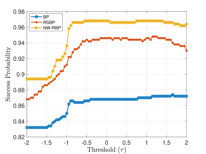
(a) Success Probability vs. Threshold ($\tau$)

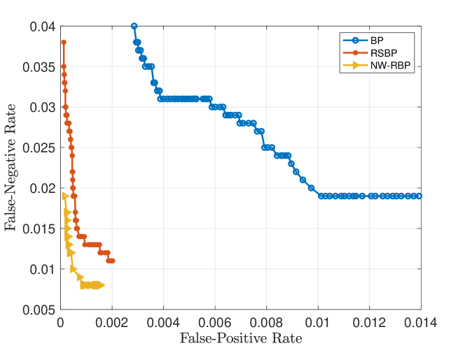
(b) False-Negative Rate vs. False-Positive Rate

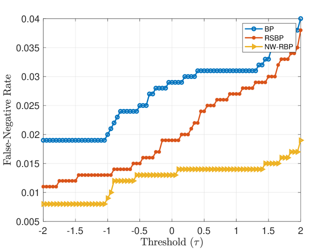
(c) False-Negative Rate vs. Threshold ($\tau$)

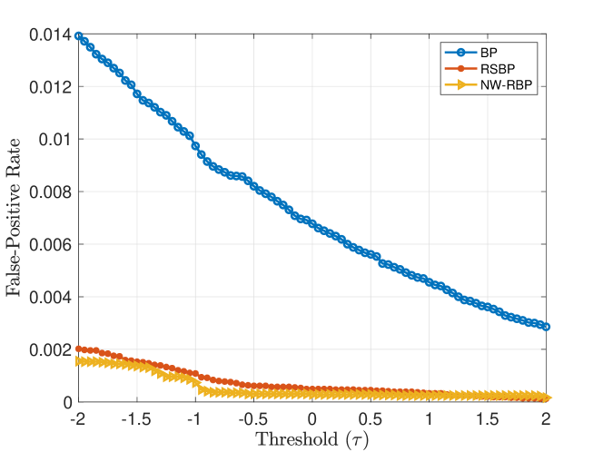
(d) False-Positive Rate vs. Threshold ($\tau$)

Figure 2: The performance of different decoding algorithms for different values of the threshold $\tau$.

References

- [1] A. Ganesan, S. Jaggi, and V. Saligrama, “Learning immune-defectives graph through group tests,” IEEE Transactions on Information Theory, vol. 63, no. 5, pp. 3010–3028, 2017.
- [2] A. Sharma and C. R. Murthy, “Group testing-based spectrum hole search for cognitive radios,” IEEE Transactions on Vehicular Technology, vol. 63, no. 8, pp. 3794–3805, 2014.
- [3] H. A. Inan, P. Kairouz, and A. Özgür, “Sparse combinatorial group testing,” IEEE Transactions on Information Theory, vol. 66, no. 5, pp. 2729–2742, 2020.
- [4] D. M. Malioutov, K. R. Varshney, A. Emad, and S. Dash, Learning Interpretable Classification Rules with Boolean Compressed Sensing. Cham: Springer International Publishing, 2017, pp. 95–121. [Online]. Available: https://doi.org/10.1007/978-3-319-54024-5_5
- [5] K. R. Narayanan, A. Heidarzadeh, and R. Laxminarayan, “On accelerated testing for COVID-19 using group testing,” CoRR, vol. abs/2004.04785, 2020. [Online]. Available: https://arxiv.org/abs/2004.04785
- [6] B. Abdalhamid, C. R. Bilder, E. L. McCutchen, S. H. Hinrichs, S. A. Koepsell, and P. C. Iwen, “Assessment of Specimen Pooling to Conserve SARS CoV-2 Testing Resources,” American Journal of Clinical Pathology, vol. 153, no. 6, pp. 715–718, 04 2020. [Online]. Available: https://doi.org/10.1093/ajcp/aqaa064
- [7] M. Aldridge, “Conservative two-stage group testing,” 2020.
- [8] N. Shental, S. Levy, V. Wuvshet, S. Skorniakov, B. Shalem, A. Ottolenghi, Y. Greenshpan, R. Steinberg, A. Edri, R. Gillis, M. Goldhirsh, K. Moscovici, S. Sachren, L. M. Friedman, L. Nesher, Y. Shemer-Avni, A. Porgador, and T. Hertz, “Efficient high-throughput sars-cov-2 testing to detect asymptomatic carriers,” Science Advances, vol. 6, no. 37, 2020. [Online]. Available: https://advances.sciencemag.org/content/6/37/eabc5961
- [9] E. Karimi, F. Kazemi, A. Heidarzadeh, K. R. Narayanan, and A. Sprintson, “Sparse graph codes for non-adaptive quantitative group testing,” in 2019 IEEE Information Theory Workshop (ITW), 2019, pp. 1–5.
- [10] H. A. Inan, P. Kairouz, M. Wootters, and A. Ozgur, “On the optimality of the kautz-singleton construction in probabilistic group testing,” in 2018 56th Annual Allerton Conference on Communication, Control, and Computing (Allerton), 2018, pp. 188–195.
- [11] P. Nikolopoulos, T. Guo, C. Fragouli, and S. N. Diggavi, “Community aware group testing,” CoRR, vol. abs/2007.08111, 2020. [Online]. Available: https://arxiv.org/abs/2007.08111
- [12] E. Karimi, F. Kazemi, A. Heidarzadeh, and A. Sprintson, “A simple and efficient strategy for the coin weighing problem with a spring scale,” in 2018 IEEE International Symposium on Information Theory (ISIT), June 2018, pp. 1730–1734.
- [13] E. Karimi, F. Kazemi, A. Heidarzadeh, K. R. Narayanan, and A. Sprintson, “Non-adaptive quantitative group testing using irregular sparse graph codes,” in 2019 57th Annual Allerton Conference on Communication, Control, and Computing (Allerton), 2019, pp. 608–614.
- [14] S. Ahn, W. Chen, and A. Özgür, “Adaptive group testing on networks with community structure,” CoRR, vol. abs/2101.02405, 2021. [Online]. Available: https://arxiv.org/abs/2101.02405
- [15] M. Aldridge, O. Johnson, and J. Scarlett, “Group testing: An information theory perspective,” Foundations and Trends® in Communications and Information Theory, vol. 15, no. 3-4, pp. 196–392, 2019. [Online]. Available: http://dx.doi.org/10.1561/0100000099
- [16] A. I. V. Casado, M. Griot, and R. D. Wesel, “Informed dynamic scheduling for belief-propagation decoding of ldpc codes,” in 2007 IEEE International Conference on Communications, 2007, pp. 932–937.
- [17] P. Radosavljevic, A. de Baynast, and J. Cavallaro, “Optimized message passing schedules for ldpc decoding,” in Conference Record of the Thirty-Ninth Asilomar Conference onSignals, Systems and Computers, 2005., 2005, pp. 591–595.