An Unconstrained Convex Formulation of Compliant Contact

Abstract

We present a convex formulation of compliant frictional contact and a robust, performant method to solve it in practice. By analytically eliminating contact constraints, we obtain an unconstrained convex problem. Our solver has proven global convergence and warm-starts effectively, enabling simulation at interactive rates. We develop compact analytical expressions of contact forces allowing us to describe our model in clear physical terms and to rigorously characterize our approximations. Moreover, this enables us not only to model point contact, but also to incorporate sophisticated models of compliant contact patches. Our time stepping scheme includes the midpoint rule, which we demonstrate achieves second order accuracy even with frictional contact. We introduce a number of accuracy metrics and show our method outperforms existing commercial and open source alternatives without sacrificing accuracy. Finally, we demonstrate robust simulation of robotic manipulation tasks at interactive rates, with accurately resolved stiction and contact transitions, as required for meaningful sim-to-real transfer. Our method is implemented in the open source robotics toolkit Drake.

I Introduction

Simulation of multibody systems with frictional contact has proven indispensable in robotics, aiding at multiple stages during the mechanical and control design, testing, and training of robotic systems. Robotic applications often require robust simulation tools that can perform at interactive rates without sacrificing accuracy, a critical prerequisite for meaningful sim-to-real transfer. However, reliable modeling and simulation for contact-rich robotic applications remains somewhat elusive.

Rigid body dynamics with frictional contact is complicated by the non-smooth nature of the solutions. It is well known [1] that rigid contact when combined with the Coulomb model of friction can lead to paradoxical configurations for which solutions in terms of accelerations and forces do not exist. These phenomena are known as Painlevé paradoxes [2].

Figure 1: Keyframes of a dual arm manipulation task in simulation (see supplemental video). The robot is commanded to pick up a jar full of marbles, open it, pour its contents into a bowl, close the lid and place the empty jar back in place. This is a computationally intensive simulation with 160 degrees of freedom and hundreds of contact constraints per time step (see Fig. 18). Our SAP solver is robust and warm-starts effectively, enabling this simulation to run at interactive rates.

Theory resolves these paradoxes by allowing discrete velocity jumps and impulsive forces, formally casting the problem as a differential variational inequality [3]. In practice, event based approaches can resolve impulsive transitions [4], though it is not clear how to reliably detect these events even for simple one degree of freedom systems [2].

Nevertheless, the problem can be solved in a weaker formulation at the velocity level using a time-stepping scheme where the next step velocities and impulses are the unknowns at each time step [5, 6]. These formulations lead in general to a non-linear complementarity problem (NCP). A linear complementarity problem (LCP) can be formulated using a polyhedral approximation of the friction cone, though at the expense of non-physical anisotropy [7]. Even though LCP formulations guarantee solution existence [6, 8], solving them accurately and efficiently has remained difficult in practice. This has been explained partly due to the fact that these formulations are equivalent to nonconvex problems in global optimization, which are generally NP-hard [9]. Indeed, popular direct methods based on Lemke’s pivoting algorithm to solve LCPs may exhibit exponential worst-case complexity [10]. Similarly, popular iterative methods based on projected Gauss-Seidel (PGS) [11, 12] have also shown exponentially slow convergence [13]. These observations are not just of theoretical value—in practice, these methods are numerically brittle and lack robustness when tasked with computing contact forces. Software typically attempts to compensate for this inherent lack of stability and robustness through non-physical constraint relaxation and stabilization, requiring a significant amount of application-specific parameter tuning.

I-A Previous Work on Convex Approximations of Contact

To improve computational tractability, Anitescu introduced a convex relaxation of the contact problem [14]. This relaxation is a convex approximation with proven convergence to the solution of a measure differential inclusion as the time step goes to zero. For sliding contacts, the convex approximation introduces a gliding artifact at a distance $\phi$ that is proportional to the time step $\delta t$, friction coefficient $\mu$ and sliding velocity $\|{\bm{v}}_{t}\|$ [15], i.e. $\phi\sim\delta t\mu\|{\bm{v}}_{t}\|$. This artifact can be irrelevant for problems with lubricated contacts (as in many mechanisms) and goes away for sticking contacts (dominant in robotic manipulation). For sliding contact, the approximation can be adequate for applications for which the product $\delta t\mu\|{\bm{v}}_{t}\|$ is usually sufficiently small. For trajectory optimization, Todorov [16] introduces regularization into Anitescu’s formulation in order to write a strictly convex formulation with a unique, smooth and invertible solution. For simulation, Todorov [17] uses regularization to introduce numerical compliance that provides Baumgarte-like stabilization to avoid constraint drift. As a side effect, the regularized formulation can lead to a noticeable non-zero slip velocity even during stiction [18].

I-B Available Software

Even though these formulations introduce a tractable approximation of frictional contact, they have not been widely adopted in practice. We believe this is because of the lack of robust solution methods with a computational cost suitable for interactive simulation. Software such as ODE [19], Dart [20] and Vortex [21] use a polyhedral approximation of the friction cone leading to an LCP formulation. Algoryx [22] uses a split solver, reminiscent of one iteration in the staggered projections method [9]. RaiSim [23] implements an iterative method with exact solution per-contact, a significant improvement over the popular PGS used in computer graphics, though still with no convergence nor accuracy guarantees. Drake [24] solves compliant contact with regularized friction with its transition aware solver TAMSI [25].

To our knowledge, Chrono [26], Mujoco [27] and Siconos [28] are the only packages that implement the convex approximation of contact. Chrono implements a variety of solvers for Anitescu’s convex formulation [14] including projected Jacobi and Gauss-Seidel methods [29], Accelerated Projected Gradient Descent (APGD) [30], Spectral Projected Gradients (SPG) [31] and more recently Alternating Direction Method of Multipliers (ADMM) [32]. Though these methods are first order and often exhibit slow convergence, they are amenable to parallelization and have been applied successfully in the simulation of granular flows with millions of bodies. MuJoCo targets robotic applications. Its contact model is parameterized by a daunting number of non-physical parameters aimed at regularizing the problem, though at the expense of drift artifacts [18]. Still, it has become very popular in the reinforcement learning community given its performance. Siconos is an open-source software targeting large scale simulation of both rigid and deformable objects. The authors of Siconos perform an exhaustive benchmarking campaign in [33] using the convex approximation of contact. The analysis reveals that there is no universal solver and that every solver technology suffers from accuracy, robustness and/or efficiency problems.

I-C Outline and Novel Contributions

It is not clear if these convex approximations present a real advantage when compared to approaches solving the original non-convex NCP problem and whether the artifacts introduced by the approximation are acceptable for robotics applications. In this work, we propose a new unconstrained convex approximation and discuss techniques for its efficient implementation. We carefully quantify the artifacts introduced by the convex approximation and evaluate the robustness and accuracy of our method on a family of examples.

We introduce a two-stage time stepping approach (Section II-C) that allows us to incorporate both first and second order schemes such as the midpoint rule. In Section VI-B we demonstrate that the midpoint rule can achieve second order accuracy even in problems with frictional contact. Unlike previous work [34, 17] that formulates the problem in its dual form (impulses), we write a primal formulation of compliant contact in velocities (Section III-A). We then analytically eliminate constraints from this formulation to obtain an unconstrained convex problem (Section III-C).

To solve this formulation, we develop SAP—the Semi-Analytic Primal solver—in Section IV and study its theoretical and practical convergence. Crucially, we show that SAP globally converges from all initial conditions (Appendix E) and warm-starts effectively using the previous time-step velocities, enabling simulation at interactive rates.

To address accuracy and model validity, Section V-A provides compact analytic formulae for the impulses that correspond to the optimal velocities of the convex approximation. This provides intuition for the approximation, even to those without optimization expertise. Moreover, the artifacts introduced by the approximation become apparent and can be characterized precisely. We provide an exact mapping between the regularization introduced by Todorov [17] to physical parameters of compliance. Therefore regularization is no longer treated as a tuning parameter of the algorithm but as a true physical parameterization of the contact model. This allows us to incorporate not only compliant point contact, but also complex models of compliant surface patches [35, 36], as we demonstrate in Section VI-D.

We demonstrate the effectiveness of our approach in Section VI in a number of simulation cases, including the simulation of the challenging dual arm manipulation task shown in Fig. 1. We evaluate the accuracy, robustness and performance of SAP against available commercial and open-source optimization solvers.

Finally, we discuss extensions and variations in Section VII, limitations in Section VIII and conclude with final remarks in Section IX.

II Multibody Dynamics with Contact

We use generalized coordinates (in particular joint coordinates) to describe our multibody system. Therefore, the state is fully specified by the generalized positions ${\mathbf{q}}\in\mathbb{R}^{n_{q}}$ and the generalized velocities ${\mathbf{v}}\in\mathbb{R}^{n_{v}}$, where $n_{q}$ and $n_{v}$ denote the number of generalized positions and velocities, respectively. Time derivatives of the configurations relate to generalized velocities by the kinematic map ${\mathbf{N}}({\mathbf{q}})\in\mathbb{R}^{n_{q}\times n_{v}}$ as

$$\dot{{\mathbf{q}}}={\mathbf{N}}({\mathbf{q}}){\mathbf{v}}.$$ (1)

II-A Contact Kinematics

Given a configuration ${\mathbf{q}}$ of the system, we assume our geometry engine reports a set $\mathscr{C}({\mathbf{q}})$ of $n_{c}$ potential contacts between pairs of bodies. We characterize the $i\text{-th}$ contact pair in $\mathscr{C}({\mathbf{q}})$ by the location ${\bm{p}}_{i}$ of the contact point, a normal direction $\hat{{\bm{n}}}_{i}$ and signed distance function [37, 38] $\phi_{i}({\mathbf{q}})\in\mathbb{R}$, defined negative for overlapping bodies. The kinematics of each contact is further completed with the relative velocity ${\bm{v}}_{c,i}\in\mathbb{R}^{3}$ between these two bodies at point ${\bm{p}}_{i}$, expressed in a contact frame $C_{i}$ for which we arbitrarily choose the $z\text{-axis}$ to coincide with the contact normal $\hat{{\bm{n}}}_{i}$. In this frame the normal and tangential components of ${\bm{v}}_{c,i}$ are given by $v_{n,i}=\hat{{\bm{n}}}_{i}\cdot{\bm{v}}_{c,i}$ and ${\bm{v}}_{t,i}={\bm{v}}_{c,i}-v_{n,i}\hat{{\bm{n}}}_{i}$ respectively, so that ${\bm{v}}_{c,i}=[{\bm{v}}_{t,i}\,v_{n,i}]$.

We form the vector ${\mathbf{v}}_{c}\in\mathbb{R}^{3n_{c}}$ of contact velocities by stacking velocities ${\bm{v}}_{c,i}$ of all contact pairs together. In general, unless otherwise specified, we use bold italics for vectors in $\mathbb{R}^{3}$ and non-italics bold for their stacked counterparts. The generalized velocities ${\mathbf{v}}$ and contact velocities ${\mathbf{v}}_{c}$ satisfy the equation ${\mathbf{v}}_{c}={\mathbf{J}}\,{\mathbf{v}}$, where ${\mathbf{J}}({\mathbf{q}})\in\mathbb{R}^{3n_{c}\times n_{v}}$ denotes the contact Jacobian.

II-B Contact Modeling

We model the normal component of the impulse $\gamma_{n}$ during a time interval of size $\delta t$ with the compliant law

$$\gamma_{n}/\delta t=(-k\phi-\tau_{d}\,k\,v_{n})_{+}$$ (2)

where $k$ is the stiffness parameter, $\tau_{d}$ is a dissipation time scale and $(x)_{+}=\max(0,x)$ is the positive part operator. The $\delta t$ is needed to convert forces into impulses. This model of compliance can be written as the equivalent complementarity condition

$$0\leq\phi+\tau_{d}\,v_{n}+\frac{c}{\delta t}\gamma_{n}\perp\gamma_{n}\geq 0$$ (3)

where $c=k^{-1}$ is the compliance parameter and $0\leq a\perp b\geq 0$ denotes complementarity, i.e. $a\geq 0$, $b\geq 0$ and $a\,b=0$.

The tangential component ${\bm{\gamma}}_{t}\in\mathbb{R}^{2}$ of the contact impulse is modeled with Coulomb’s law of dry friction as

$${\bm{\gamma}}_{t}=\operatorname*{arg\,min}_{\|{\bm{\xi}}\|\leq\mu\gamma_{n}}{\bm{v}}_{t}\cdot{\bm{\xi}}$$ (4)

where $\mu>0$ is the coefficient of friction. Equation (4) describes the maximum dissipation principle, which states that friction impulses maximize the rate of energy dissipation. In other words, friction impulses oppose the sliding velocity direction. Moreover, (4) states that contact impulses ${\bm{\gamma}}$ are constrained to be in the friction cone $\mathcal{F}=\{[{\bm{x}}_{t},x_{n}]\in\mathbb{R}^{3}\,|\,\|{\bm{x}}_{t}\|\leq\mu x_{n}\}$. The optimality conditions for Eq. (4) are [39, 29]

$$\mu\gamma_{n}{\bm{v}}_{t}+\lambda{\bm{\gamma}}_{t}={\bm{0}}$$

$$0\leq\lambda\perp\mu\gamma_{n}-\|{\bm{\gamma}}_{t}\|\geq 0$$ (5)

where $\lambda$ is the multiplier needed to enforce Coulomb’s law condition $\|{\bm{\gamma}}_{t}\|\leq\mu\gamma_{n}$. Notice that in the form we write Eq. (5), multiplier $\lambda$ is zero during stiction and takes the value $\lambda=\|{\bm{v}}_{t}\|$ during sliding. Finally, the total contact impulse ${\bm{\gamma}}\in\mathbb{R}^{3}$ expressed in the contact frame $C$ is given by ${\bm{\gamma}}=[{\bm{\gamma}}_{t}\,\gamma_{n}]$.

II-C Discrete Model

We base our time-stepping scheme on the $\theta\text{-method}$ [40, §II.7]. We discretize time into intervals of fixed size $\delta t$ and seek to advance the state of the system from time $t^{n}$ to the next step at $t^{n+1}=t^{n}+\delta t$. In the $\theta\text{-method}$, variables are evaluated at intermediate time steps $t^{\theta}=\theta t^{n+1}+(1-\theta)t^{n}$, with $\theta\in[0,1]$. We define mid-step quantities ${\mathbf{q}}^{\theta}$, ${\mathbf{v}}^{\theta}$, and ${\mathbf{v}}^{\theta_{vq}}$ in accordance with the standard $\theta\text{-method}$ using scalar parameters $\theta$ and $\theta_{vq}$

$${\mathbf{q}}^{\theta} \stackrel{{\scriptstyle\text{\tiny def}}}{{=}}\theta{\mathbf{q}}+(1-\theta){\mathbf{q}}_{0},$$

$${\mathbf{v}}^{\theta} \stackrel{{\scriptstyle\text{\tiny def}}}{{=}}\theta{\mathbf{v}}+(1-\theta){\mathbf{v}}_{0},$$

$${\mathbf{v}}^{\theta_{vq}} \stackrel{{\scriptstyle\text{\tiny def}}}{{=}}\theta_{vq}{\mathbf{v}}+(1-\theta_{vq}){\mathbf{v}}_{0},$$ (6)

where, to simplify notation, we use the naught subscript to denote quantities evaluated at the previous time step $t^{n}$ while no additional subscript is used for quantities at the next time step $t^{n+1}$. Using these definitions we write the following time stepping scheme where the unknowns are the next time step generalized velocities ${\mathbf{v}}\in\mathbb{R}^{n_{v}}$, impulses ${\bm{\gamma}}\in\mathbb{R}^{3n_{c}}$ and multipliers ${\bm{\lambda}}\in\mathbb{R}^{n_{c}}$

$${\mathbf{M}}({\mathbf{q}}^{\theta}({\mathbf{v}}))({\mathbf{v}}-{\mathbf{v}}_{0})=$$

$$\qquad\delta t\,{\mathbf{k}}({\mathbf{q}}^{\theta}({\mathbf{v}}),{\mathbf{v}}^{\theta}({\mathbf{v}}))+{\mathbf{J}}({\mathbf{q}}_{0})^{T}{\mathbf{{\bm{\gamma}}}},$$ (7)

$$0\leq\phi_{i}({\mathbf{q}}({\mathbf{v}}))+\tau_{d,i}\,v_{n,i}({\mathbf{q}},{\mathbf{v}})+\frac{c_{i}}{\delta t}\gamma_{n,i}$$

$$\qquad\perp\gamma_{n,i}\geq 0,\quad\qquad\qquad\qquad i\in\mathscr{C}({\mathbf{q}}_{0})$$ (8)

$$\mu_{i}\gamma_{n,i}{\bm{v}}_{t,i}({\mathbf{q}},{\mathbf{v}})+\lambda_{i}{\bm{\gamma}}_{t,i}={\bm{0}},\!\qquad i\in\mathscr{C}({\mathbf{q}}_{0})$$ (9)

$$0\leq\lambda_{i}\perp\mu_{i}\gamma_{n,i}-\|{\bm{\gamma}}_{t,i}\|\geq 0,\!\!\qquad i\in\mathscr{C}({\mathbf{q}}_{0})$$ (10)

$$\dot{{\mathbf{q}}}^{\theta_{vq}}({\mathbf{v}})={\mathbf{N}}({\mathbf{q}}^{\theta}({\mathbf{v}})){\mathbf{v}}^{\theta_{vq}}({\mathbf{v}}),$$ (11)

$${\mathbf{q}}({\mathbf{v}})={\mathbf{q}}_{0}+\delta t\dot{{\mathbf{q}}}^{\theta_{vq}}({\mathbf{v}}),$$ (12)

where ${\mathbf{M}}({\mathbf{q}})\in\mathbb{R}^{n_{v}\times n_{v}}$ is the mass matrix and ${\mathbf{k}}({\mathbf{q}},{\mathbf{v}})\in\mathbb{R}^{n_{v}}$ models external forces such as gravity, gyroscopic terms and other smooth generalized forces such as those arising from springs and dampers.

This scheme includes some of the most popular schemes for forward dynamics:

• Explicit Euler with $\theta=\theta_{vq}=0$,

• Symplectic Euler with $\theta=0$ and $\theta_{vq}=1$,

• Implicit Euler with $\theta=\theta_{vq}=1$, and

• Symplectic midpoint rule, which is second order, with $\theta=\theta_{vq}=1/2$.

Notice that in our version of the $\theta\text{-method}$, the additional parameter $\theta_{vq}$ allows us to also incorporate the popular Symplectic Euler scheme.

When only conservative forces are considered in ${\mathbf{k}}({\mathbf{q}},{\mathbf{v}})$, the symplectic Euler scheme keeps the total mechanical energy bounded while exact energy conservations can be attained with the second order midpoint rule, see results in Section VI-B. In addition, stability analysis in [41, 42] shows that these implicit schemes are appropriate for the integration of stiff forces arising in multibody applications such as springs and dampers.

II-D Two-Stage Scheme

Similar to the work in [43] for the simulation of deformable objects and to projection methods used in fluid mechanics [44], we solve Eqs. (7)-(12) in two stages. In the first stage, we solve for the free motion velocities ${\mathbf{v}}^{*}$ the system would have in the absence of contact constraints, according to

$${\mathbf{m}}({\mathbf{v}}^{*}) ={\mathbf{0}},$$ (13)

where we define the momentum residual ${\mathbf{m}}({\mathbf{v}})$ from Eq. (7) as

$${\mathbf{m}}({\mathbf{v}})={\mathbf{M}}({\mathbf{q}}^{\theta}({\mathbf{v}}))({\mathbf{v}}-{\mathbf{v}}_{0})-\delta t\,{\mathbf{k}}({\mathbf{q}}^{\theta}({\mathbf{v}}),{\mathbf{v}}^{\theta}({\mathbf{v}})).$$ (14)

For integration schemes that are implicit in ${\mathbf{v}}^{*}$ (e.g. the implicit Euler scheme and the midpoint rule), we solve Eq. (13) with Newton’s method. For schemes explicit in ${\mathbf{v}}^{*}$, only the mass matrix ${\mathbf{M}}$ needs to be inverted, which can be accomplished efficiently using the $\mathcal{O}(n)$ Articulated Body Algorithm [45].

The second stage solves a linear approximation of the balance of momentum in Eq. (7) about ${\mathbf{v}}^{*}$ that satisfies the contact constraints, Eqs. (8)-(10). To write a convex formulation of contact in Section III, our linearization uses a symmetric positive definite (SPD) approximation of the Jacobian $\partial{\mathbf{m}}/\partial{\mathbf{v}}$. To achieve this, we split the non-contact forces ${\mathbf{k}}$ in Eq. (7) as

$${\mathbf{k}}({\mathbf{q}},{\mathbf{v}})={\mathbf{k}}_{1}({\mathbf{q}},{\mathbf{v}})+{\mathbf{k}}_{2}({\mathbf{q}},{\mathbf{v}}),$$

such that the Jacobians $\partial{\mathbf{k}}_{1}/\partial{\mathbf{q}}$ and $\partial{\mathbf{k}}_{1}/\partial{\mathbf{v}}$ are negative definite matrices while the same is generally not true for the Jacobians of ${\mathbf{k}}_{2}$. The term ${\mathbf{k}}_{1}({\mathbf{q}},{\mathbf{v}})$ can include forces from modeling elements such as spring and dampers. The term ${\mathbf{k}}_{2}({\mathbf{q}},{\mathbf{v}})$ includes all other contributions that cannot guarantee negative definiteness of their Jacobians, such as Coriolis and gyroscopic forces arising in multibody dynamics with generalized coordinates. We can now define the SPD approximation of $\partial{\mathbf{m}}/\partial{\mathbf{v}}$ evaluated at ${\mathbf{v}}^{*}$ as

$${\mathbf{A}} ={\mathbf{M}}+\delta t^{2}\,\theta\theta_{qv}{\mathbf{K}}+\delta t\,\theta{\mathbf{D}},$$ (15)

$${\mathbf{K}} =-\frac{\partial{\mathbf{k}}_{1}}{\partial{\mathbf{q}}}\frac{\partial\dot{{\mathbf{q}}}^{\theta_{vq}}}{\partial{\mathbf{v}}},$$ (16)

$${\mathbf{D}} =-\frac{\partial{\mathbf{k}}_{1}}{\partial{\mathbf{v}}},$$ (17)

where ${\mathbf{K}}\succ 0$ and ${\mathbf{D}}\succ 0$ are the stiffness and damping matrices of the system, respectively. For joint level spring-dampers models, ${\mathbf{K}}$ and ${\mathbf{D}}$ are constant, diagonal, and positive definite matrices. Section VI-B shows the performance of our scheme for a system with a linear spring.

Using this SPD approximation of $\partial{\mathbf{m}}/\partial{\mathbf{v}}$, the linearized balance of momentum (7) reads

$${\mathbf{A}}({\mathbf{v}}-{\mathbf{v}}^{*})={\mathbf{J}}^{T}{\mathbf{{\bm{\gamma}}}},$$ (18)

where for convenience we use ${\mathbf{J}}$ as a shorthand to denote ${\mathbf{J}}({\mathbf{q}}_{0})$. The approximation in Eq. (18) and the original discrete momentum update in Eq. (7) agree to second order as shown by the following result, proved in Appendix A.

Proposition 1.

Matrix ${\mathbf{A}}$ is a first order approximation to the Jacobian of ${\mathbf{m}}$, i.e.,

$$\left.\frac{\partial{\mathbf{m}}}{\partial{\mathbf{v}}}\right|_{{\mathbf{v}}={\mathbf{v}}^{*}}={\mathbf{A}}+\mathcal{O}(\delta t).$$

Therefore, Eq. (18) is a second order approximation of the discrete balance of momentum in Eq. (7). Moreover, ${\mathbf{A}}\succ 0$.

Notice that, in the absence of constraint impulses, the velocities at the next time step are equal to the free motion velocities, i.e., ${\mathbf{v}}={\mathbf{v}}^{*}$, and they are computed with the order of accuracy of the $\theta\text{-method}$. Furthermore, we also expect to recover the properties of the $\theta\text{-method}$ when contact constraints are in stiction. As an example, for bodies in contact that are under rolling friction, the contact constraints behave as bi-lateral constraints that impose zero slip velocity. In this case, our two-stage method with the midpoint rule exhibits considerably less numerical dissipation than first order methods (see results in Section VI-B.)

Even after the linearization of the balance of momentum in Eq. (18), the full problem with the contact constraints (8)-(10) still consists of a non-convex nonlinear complementarity problem (NCP). This kind of problems are difficult to solve in practice, especially so in engineering applications for which robustness and accuracy are required. In the next section we introduce a number of approximations to this original NCP that allow us to make the problem tractable and solve it efficiently in practice.

III Convex Approximation of Contact Dynamics

In this section we build from previous work on convex approximations of contact [14, 16, 17] to write a new convex formulation of compliant contact in terms of velocities.

III-A Primal Formulation

We introduce a new decision variable ${\bm{\sigma}}\in\mathbb{R}^{3n_{c}}$ and set up our convex formulation of compliant contact as the following optimization problem

$$\min_{{\mathbf{v}},{\bm{\sigma}}} \ell_{p}({\mathbf{v}},{\bm{\sigma}})=\frac{1}{2}\|{\mathbf{v}}-{\mathbf{v}}^{*}\|_{A}^{2}+\frac{1}{2}\|{\bm{\sigma}}\|_{R}^{2}$$ (19)

s.t. $${\mathbf{g}}=({\mathbf{J}}{\mathbf{v}}-\hat{{\mathbf{v}}}_{c}+{\mathbf{R}}{\bm{\sigma}})\in\mathcal{F}^{*},$$

where $\|{\mathbf{z}}\|_{X}^{2}={\mathbf{z}}^{T}{\mathbf{X}}{\mathbf{z}}$ with ${\mathbf{X}}\succ 0$ and $\mathcal{F^{*}}=\mathcal{F}^{*}_{1}\times\mathcal{F}^{*}_{2}\times\cdots\times\mathcal{F}^{*}_{n_{c}}$ is the dual cone of the friction cone $\mathcal{F}=\mathcal{F}_{1}\times\mathcal{F}_{2}\times\cdots\times\mathcal{F}_{n_{c}}$, with $\times$ the Cartesian product. The positive diagonal matrix ${\mathbf{R}}\in\mathbb{R}^{3n_{c}\times 3n_{c}}$ and the vector of stabilization velocities $\hat{{\mathbf{v}}}_{c}$ encode the problem data needed to model compliant contact. We establish a very clear physical meaning for these terms in Section V-A. We note that when $R$ and ${\bm{\sigma}}$ are removed, this reformulation reduces to [15].

We refer to (19) as the primal formulation and next derive its dual. To begin, define the Lagrangian

$$\mathcal{L}({\mathbf{v}},{\bm{\sigma}},{\bm{\gamma}})=\frac{1}{2}\|{\mathbf{v}}-{\mathbf{v}}^{*}\|_{A}^{2}+\frac{1}{2}\|{\bm{\sigma}}\|_{R}^{2}-{\bm{\gamma}}^{T}{\mathbf{g}},$$ (20)

where ${\bm{\gamma}}\in\mathcal{F}$ is the dual variable for the constraint ${\bm{g}}\in\mathcal{F}^{*}$. Taking gradients of the Lagrangian with respect to ${\mathbf{v}}$ and ${\bm{\sigma}}$ leads to the optimality conditions

$${\mathbf{A}}({\mathbf{v}}-{\mathbf{v}}^{*}) ={\mathbf{J}}^{T}{\bm{\gamma}}$$ (21a)

$${\bm{\sigma}} ={\bm{\gamma}}.$$ (21b)

Note that (21a) is a restatement of the balance of momentum (18) if the dual variable ${\bm{\gamma}}$ is interpreted as a vector of contact impulses. Using the optimality condition (21b) to eliminate ${\bm{\sigma}}$ from the Lagrangian yields the dual formulation

$$\min_{{\bm{\gamma}}\in\mathcal{F}}\ell_{d}({\bm{\gamma}})=\frac{1}{2}{\bm{\gamma}}^{T}(\mathbf{W}+\mathbf{R}){\bm{\gamma}}+{\bm{r}}^{T}{\bm{\gamma}},$$ (22)

where ${\mathbf{W}}={\mathbf{J}}{\mathbf{A}}^{-1}{\mathbf{J}}^{T}$ is the Delassus operator and ${\mathbf{r}}={\mathbf{v}}_{c}^{*}-\hat{{\mathbf{v}}}_{c}$ with ${\mathbf{v}}_{c}^{*}={\mathbf{J}}{\mathbf{v}}^{*}$. In summary, we have proven the following theorem.

Theorem 1.

The dual of (19) is given by (22). Moreover, when $\{{\mathbf{v}},{\bm{\sigma}}\}$ is primal optimal and ${\bm{\gamma}}$ is dual optimal, ${\bm{\sigma}}={\bm{\gamma}}$.

Finally, we note that the dual (22) is equivalent to the formulation in [16] when $\theta=0$ in Eq. (7) and ${\mathbf{A}}={\mathbf{M}}({\mathbf{q}}_{0})$.

III-B Analytical Inverse Dynamics

The dual optimal impulses of (22) can be constructed from the primal optimal velocities of (19) using a simple projection operation. Following [17], we call this construction analytical inverse dynamics. Moreover, this projection decomposes into a set of individual projections for each contact impulse ${\bm{\gamma}}_{i}$ given the separable structure of the constraints. Letting ${\bm{y}}_{i}({\bm{v}}_{c,i})=-{\bm{R}}_{i}^{-1}({\bm{v}}_{c,i}-\hat{{\bm{v}}}_{c,i})$, these projections take the form

$${\bm{\gamma}}_{i}({\bm{v}}_{c,i}) =P_{\mathcal{F}_{i}}({\bm{y}}_{i}({\bm{v}}_{c,i}))$$ (23)

$$=\operatorname*{arg\,min}_{{\bm{\gamma}}\in\mathcal{F}_{i}}\quad\frac{1}{2}({\bm{\gamma}}-{\bm{y}}_{i})^{T}{\bm{R}}_{i}({\bm{\gamma}}-{\bm{y}}_{i}),$$

where ${\bm{R}}_{i}\in\mathbb{R}^{3\times 3}$ is the $i\text{-th}$ diagonal block of the regularization matrix ${\mathbf{R}}$. That is, ${\bm{\gamma}}_{i}$ is the projection $P_{\mathcal{F}_{i}}$ of ${\bm{y}}_{i}({\bm{v}}_{c,i})$ onto the friction cone $\mathcal{F}_{i}$ using the norm defined by ${\bm{R}}_{i}$. Remarkably, the projection map $P_{\mathcal{F}_{i}}$ can be evaluated analytically. We provide algebraic expressions for it in Section V-A and derivations in Appendix C. The projection $P_{\mathcal{F}}({\mathbf{y}})$ onto the full cone $\mathcal{F}:=\mathcal{F}_{1}\times\mathcal{F}_{2}\times\cdots\times\mathcal{F}_{n_{c}}$ is obtained by simply stacking together the individual projections $P_{\mathcal{F}_{i}}({\bm{y}}_{i})$ from Eq. (23), where we form ${\mathbf{y}}$ by stacking together each ${\bm{y}}_{i}$ from all contact pairs. In this notation, the optimal impulse ${\bm{\gamma}}$ of (22) and the optimal velocities ${\mathbf{v}}$ of (19) satisfy ${\bm{\gamma}}=P_{\mathcal{F}}({\mathbf{y}}({\mathbf{v}}))$.

III-C An Unconstrained Convex Formulation

We use the analytical ${\bm{\gamma}}=P_{\mathcal{F}}({\mathbf{y}}({\mathbf{v}}))$ from Section III-B and the optimality condition ${\bm{\sigma}}={\bm{\gamma}}$ from Theorem 1 to eliminate both ${\bm{\sigma}}$ and the constraints from the primal formulation (19). In total, we obtain the following unconstrained problem in velocities only

$$\min_{{\mathbf{v}}}\ell_{p}({\mathbf{v}})=\frac{1}{2}\|{\mathbf{v}}-{\mathbf{v}}^{*}\|_{A}^{2}+\frac{1}{2}\|P_{\mathcal{F}}({\mathbf{y}}({\mathbf{v}}))\|_{R}^{2}.$$ (24)

Correctness of this reformulation is asserted by the following theorem, which we prove in Appendix B.

Theorem 2.

If ${\mathbf{v}}$ solves the unconstrained formulation (24), then $({\mathbf{v}},{\bm{\sigma}})$, with ${\bm{\sigma}}=P_{\mathcal{F}}({\mathbf{y}}({\mathbf{v}}))$, solves the primal formulation (19).

Lemma 2 in Appendix E shows that the unconstrained cost $\ell_{p}({\mathbf{v}})$ is strongly convex and differentiable with Lipschitz continuous gradients. Therefore, the unconstrained formulation (24) has a unique solution, and can be efficiently solved. Section IV presents our novel SAP solver specifically designed for its solution.

We outline our time-stepping scheme in Algorithm 1.

Algorithm 1 Overall Time-Stepping Strategy

1:Solve free motion velocities from ${\mathbf{m}}({\mathbf{v}}^{*})={\mathbf{0}}$, Eq. (14)

2:Solve $\displaystyle{\mathbf{v}}=\operatorname*{arg\,min}_{{\mathbf{v}}}\ell_{p}({\mathbf{v}})$, Eq. (24)

3:Update positions $\displaystyle{\mathbf{q}}={\mathbf{q}}_{0}+\delta t{\mathbf{N}}({\mathbf{q}}^{\theta}){\mathbf{v}}^{\theta_{vq}}$, Eqs. (11)-(12)

We note that Algorithm 1 is executed once per time step, with no inner iterations updating ${\mathbf{A}}$. That is, our strategy is not solving the original, possibly nonlinear, balance of momentum (7) but its (second-order accurate) linear approximation in (18). This approximation can be exact for many multibody systems encountered in practice. For instance, joint springs and dampers contribute constant stiffness and damping matrices in (15).

IV Semi-Analytic Primal Solver

Inspired by Newton’s method, our Semi-Analytic Primal Solver (SAP) seeks to solve (24) by monotonically decreasing the primal cost $\ell_{p}({\mathbf{v}})$ at each iteration, as outlined in Algorithm 2.

Algorithm 2 The Semi-Analytic Primal Solver (SAP)

1:Initialize ${\mathbf{v}}_{m}\leftarrow{\mathbf{v}}_{0}$

2:repeat until$~{}\|\tilde{\nabla}\ell_{p}\|<\varepsilon_{a}+\varepsilon_{r}\max(\|\tilde{{\mathbf{p}}}\|,\|\tilde{{\mathbf{j}}_{c}}\|)$, Eq. (26)

3:     $\Delta{\mathbf{v}}_{m}=-{\mathbf{H}}^{-1}({\mathbf{v}}_{m})\nabla_{\mathbf{v}}\ell_{p}({\mathbf{v}}_{m})$

4:     $\displaystyle\alpha_{m}=\operatorname*{arg\,min}_{t\in\mathbb{R}^{++}}\ell_{p}({\mathbf{v}}_{m}+t\Delta{\mathbf{v}}_{m})$

5:     $\displaystyle{\mathbf{v}}_{m+1}={\bm{v}}_{m}+\alpha_{m}\Delta{\mathbf{v}}_{m}$

6:return $\{{\mathbf{v}}$, ${\bm{\gamma}}=P_{\mathcal{F}}({\bm{y}}({\mathbf{v}}))\}$

The SAP iterations require ${\mathbf{H}}({\mathbf{v}})\succ 0$ at all iterations. At points where $\nabla_{\mathbf{v}}\ell_{p}({\mathbf{v}})$ is differentiable, ${\mathbf{H}}({\mathbf{v}})$ is simply set equal to the Hessian of the cost function. In general, ${\mathbf{H}}({\mathbf{v}})$ is evaluated using a partition of its domain. For each set in the partition, $\nabla_{\mathbf{v}}\ell_{p}({\mathbf{v}})$ is differentiable on the interior, and the Hessian admits a simple formula. We globally define ${\mathbf{H}}({\mathbf{v}})$ by adopting one of these Hessian formulas on the boundary. The partition is described in Appendix C. The Hessian formula are given in Appendix D. Our convergence analysis in Appendix E also accounts for this definition.

As shown in Appendix E, SAP globally converges at least at a linear-rate. Further, SAP exhibits quadratic convergence when $\nabla^{2}\ell_{p}$ exists in a neighborhood of the optimal ${\mathbf{v}}$. In practice, we initialize SAP with the previous time-step velocity ${\mathbf{v}}_{0}$. The stopping criteria is discussed below in Section IV-E.

IV-A Gradients

We provide a detailed derivation of the gradients in Appendix D. Here we summarize the main results required for implementation. The gradient of the primal cost $\ell_{p}$ reduces to the balance of momentum

$$\nabla_{\mathbf{v}}\ell_{p}({\mathbf{v}})={\mathbf{A}}({\mathbf{v}}-{\mathbf{v}}^{*})-{\mathbf{J}}^{T}{\bm{\gamma}}({\mathbf{v}}),$$

where ${\bm{\gamma}}({\mathbf{v}})=P_{\mathcal{F}}({\bm{y}}({\mathbf{v}}))$ is given by the analytical inverse dynamics (V-A). We define matrix ${\mathbf{G}}\succeq 0$ that evaluates to $-\nabla_{{\mathbf{v}}_{c}}{\bm{\gamma}}$ where $P_{\mathcal{F}}({\mathbf{y}}({\mathbf{v}}))$ is differentiable. Otherwise ${\mathbf{G}}$ extends our analytical expressions as outlined in Appendix D. Matrix ${\mathbf{G}}$ is a block diagonal matrix where each diagonal block for the $i\text{-th}$ contact is a $3\times 3$ matrix.

In total, we evaluate ${\mathbf{H}}$ via

$${\mathbf{H}}={\mathbf{A}}+{\mathbf{J}}^{T}{\mathbf{G}}\,{\mathbf{J}},$$

which is strictly positive definite since ${\mathbf{A}}\succ 0$.

IV-B Line Search

The line search algorithm is critical to the success of SAP given that $\nabla\ell_{p}({\mathbf{v}})$ can rapidly change during contact-mode transitions. We explore two line search algorithms: an approximate backtracking line search with Armijo’s stopping criteria and an exact (to machine epsilon) line search.

At the $m\text{-th}$ Newton iteration, backtracking line search starts with a maximum step length of $\alpha_{\text{Max}}$ and progressively decreases it by a factor $\rho\in(0,1)$ as $\alpha\leftarrow\rho\alpha$ until Armijo’s criteria [46, §3.1] is satisfied. We write Armijo’s criteria as $~{}\ell_{p}({\mathbf{v}}^{m}+\alpha\Delta{\mathbf{v}}^{m})<\ell_{p}({\mathbf{v}}^{m})+c\,\alpha\,d\ell_{p}/d\alpha({\mathbf{v}}^{m})$. Typical parameters we use are $\rho=0.8$, $c=10^{-4}$ and $\alpha_{\text{Max}}=1.25$.

For the exact line search we use the method rtsafe [47, §9.4] to find the unique root of $d\ell/d\alpha$. This is a one-dimensional root finder that uses the Newton-Raphson method and switches to bisection when an iterate falls outside a search bracket or when convergence is slow. The fast computation of derivatives we show next allows us to iterate $\alpha$ to machine precision at a negligible impact on the computational cost. In practice, this is our preferred algorithm since it allows us to use very low regularization parameters without having to tune tolerances in the line search.

IV-C Efficient Analytical Derivatives For Line Search

The algorithm rtsafe requires the first and second directional derivatives of $\ell_{p}$. We show how to compute these derivatives efficiently in $\mathcal{O}(n)$ operations. Defining $\ell(\alpha)=\ell_{p}({\mathbf{v}}+\alpha\Delta{\mathbf{v}})$, we compute first and second derivatives as

$$\frac{d\ell}{d\alpha} =\Delta{\mathbf{v}}^{T}\nabla_{\mathbf{v}}\ell(\alpha),$$

$$\frac{d^{2}\ell}{d\alpha^{2}} =\Delta{\mathbf{v}}^{T}{\mathbf{H}}(\alpha)\Delta{\mathbf{v}}.$$

Using the gradients from Section IV-A, we can write

$$\frac{d\ell}{d\alpha}(\alpha)=\Delta{\mathbf{v}}^{T}{\mathbf{A}}({\mathbf{v}}(\alpha)-{\mathbf{v}}^{*})-\Delta{\mathbf{v}}^{T}{\mathbf{J}}^{T}{\bm{\gamma}}.$$

These are computed efficiently by first calculating the change in velocity $\Delta{\mathbf{v}}_{c}:={\mathbf{J}}\Delta{\mathbf{v}}$ and change of momentum $\Delta{\mathbf{p}}:={\mathbf{A}}\Delta{\mathbf{v}}$. The calculation is then completed via

$$\frac{d\ell}{d\alpha}(\alpha)=\Delta{\mathbf{p}}^{T}({\mathbf{v}}(\alpha)-{\mathbf{v}}^{*})-\Delta{\mathbf{v}}_{c}^{T}{\bm{\gamma}}(\alpha),$$

which only requires dot products that can be computed in $\mathcal{O}(n_{v})$ and $\mathcal{O}(n_{c})$ respectively. Similarly for the second derivatives

$$\frac{d^{2}\ell}{d\alpha^{2}}(\alpha)=\Delta{\mathbf{v}}^{T}\Delta{\mathbf{p}}+\Delta{\mathbf{v}}_{c}^{T}{\mathbf{G}}(\alpha)\Delta{\mathbf{v}}_{c}.$$

Notice the first term on the right can be precomputed before the line search starts, while the second term only involves $\mathcal{O}(n_{c})$ operations given the block diagonal structure of ${\mathbf{G}}$.

IV-D Problem Sparsity

The block sparsity of ${\mathbf{H}}$ is best described with an example. We organize our multibody systems as a collection of articulated tree structures, or a forest. Consider the system in Fig. 2.

Figure 2: An example of a sparsity pattern commonly encountered in the simulation of robotic mechanical systems. The graph on the right puts trees as nodes and contact patches as edges.

In this example, a robot arm mounted on a mobile base constitutes its own tree, here labeled $t_{1}$. The number of degrees of freedom of the $t\text{-th}$ tree will be denoted with $n_{t}$. A free body is a common case of a tree with $n_{t}=6$. In general, matrix ${\mathbf{A}}$ has a block diagonal structure where each diagonal block corresponds to a tree.

We define as patches a collection of contact pairs between two trees. Each contact pair corresponds to a single cone constraint in our formulation. The set of constraint indexes that belong to patch $p$ is denoted with $\mathcal{I}_{p}$ of size (cardinality) $|\mathcal{I}_{p}|=r_{p}$. Figure 2 shows the corresponding graph where nodes correspond to trees and edges correspond to patches.

Generally, the Jacobian is sparse since the relative contact velocity only involves velocities of two trees in contact, Fig. 3. Each non-zero block ${\mathbf{J}}_{pt}$ has size $3r_{p}\times n_{t}$. Since ${\mathbf{A}}$ is block diagonal, ${\mathbf{H}}$ inherits the sparsity structure of ${\mathbf{J}}^{T}{\mathbf{G}}{\mathbf{J}}$.

We exploit this structure using a supernodal Cholesky factorization [48, §9] that can take advantage of dense algebra optimizations. Implementing this factorization requires construction of a junction tree. For this we apply the algorithm in [49], using cliques of ${\mathbf{H}}$ as input. We use the implementation from the Conex solver [50].

Figure 3: Block sparsity of the contact Jacobian ${\mathbf{J}}$ and the Hessian term ${\mathbf{J}}^{T}{\mathbf{G}}{\mathbf{J}}$, for the example illustrated in Fig. 2.

The scalability of SAP, like any second-order optimization method, depends on the complexity of solving the Newton system. For dense problems, this has $\mathcal{O}(n_{v}^{3})$ complexity, where $n_{v}$ denotes the number of generalized velocities. For sparse problems the complexity can be dramatically reduced [48]. We study scalability with number of bodies in Section VI-C. Recent work on the modeling of contact rich patches [36] studies the scalability of SAP with the number of constraints.

IV-E Stopping Criteria

To assess convergence, we monitor the norm of the optimality condition for the unconstrained problem (24)

$$\nabla\ell_{p}({\mathbf{v}})={\mathbf{A}}({\mathbf{v}}-{\mathbf{v}}^{*})-{\mathbf{J}}^{T}{\bm{\gamma}}.$$

Notice that the components of $\nabla\ell_{p}$ have units of generalized momentum ${\mathbf{p}}={\mathbf{M}}{\mathbf{v}}$. Depending on the choice of generalized coordinates, the generalized momentum components may have different units. In order to weigh all components equally, we define the diagonal matrix ${\mathbf{D}}=\text{diag}({\mathbf{M}})^{-1/2}$ and perform the following change of variables

$$\tilde{\nabla}\ell_{p} ={\mathbf{D}}\nabla\ell_{p},$$

$$\tilde{{\mathbf{p}}} ={\mathbf{D}}{\mathbf{p}},$$

$$\tilde{{\mathbf{j}}}_{c} ={\mathbf{D}}{\mathbf{j}}_{c},$$ (25)

where we define the generalized contact impulse ${\mathbf{j}}_{c}={\mathbf{J}}^{T}{\bm{\gamma}}$. With this scaling, all the new tilde variables have the same units, square root of Joules. Using these definitions, we write our stopping criteria as

$$\|\tilde{\nabla}\ell_{p}\|<\varepsilon_{a}+\varepsilon_{r}\max(\|\tilde{{\mathbf{p}}}\|,\|\tilde{{\mathbf{j}}_{c}}\|).$$ (26)

where $\varepsilon_{r}$ is a dimensionless relative tolerance that we usually set in the range from $10^{-6}$ to $10^{-1}$. The absolute tolerance $\varepsilon_{a}$ is used to detect rare cases where the solution leads to no contact and no motion, typically due to external forces. We always set this tolerance to a small number, $\varepsilon_{a}=10^{-16}$.

V Contact Modeling Parameters

Thus far, ${\bm{R}}_{i}$ and $\hat{{\bm{v}}}_{c,i}$ have been treated as known problem data. This section makes an explicit connection of these quantities with physical parameters to model compliant contact with regularized friction. We seek to model compliant contact as in Eq. (2), parameterized by physical parameters: stiffness $k$ (in N/m) and dissipation time scale $\tau_{d}$ (in seconds). Therefore, users of this model only need to provide these physical parameters and regularization is computed from them. Notice this approach is different from the one in [17], where regularization is not used to model physical compliance but rather to introduce a user tunable Baumgarte-style stabilization to avoid constraint drift.

V-A Compliant Contact, Principle of Maximum Dissipation and Artifacts

Dropping subscript $i$ for simplicity, we solve the projection problem in Eq. (23) analytically in Appendix C for a regularization matrix of the form ${\bm{R}}=\text{diag}([R_{t},R_{t},R_{n}])$

$${\bm{\gamma}} = P_{\mathcal{F}}({\bm{y}})$$

$$= \begin{dcases}{\bm{y}}&\text{stiction, }y_{r}\leq\mu y_{n}\\ \begin{bmatrix}\mu\gamma_{n}\hat{{\bm{t}}}\\ \frac{1}{1+\tilde{\mu}^{2}}\left(y_{n}+\hat{\mu}y_{r}\right)\end{bmatrix}&\text{sliding, }-\hat{\mu}y_{r}<y_{n}\leq\frac{y_{r}}{\mu}\\ {\bm{0}}&\text{no contact, }y_{n}<-\hat{\mu}y_{r}\end{dcases}$$

where ${\bm{y}}_{t}$ and $y_{n}$ are the tangential and normal components of ${\bm{y}}$, $y_{r}=\|{\bm{y}}_{t}\|$ is the radial component, and $\hat{{\bm{t}}}={\bm{y}}_{t}/y_{r}$ is the unit tangent vector. We also define the coefficients $\tilde{\mu}=\mu\,(R_{t}/R_{n})^{1/2}$ and $\hat{\mu}=\mu\,R_{t}/R_{n}$ that result from the warping introduced by the metric ${\bm{R}}$.

Our compliant model of contact is defined by

$$\hat{{\bm{v}}}_{c} = \begin{bmatrix}0\\ 0\\ \hat{v}_{n}\end{bmatrix},$$

$$\hat{v}_{n} = -\frac{\phi_{0}}{\delta t+\tau_{d}},$$

where $\phi_{0}$ is the previous step signed distance reported by the geometry engine. The normal direction regularization parameters is taken as $R_{n}^{-1}=\delta tk(\delta t+\tau_{d})$. To gain physical insight into our model, we substitute ${\bm{y}}=-{\bm{R}}^{-1}({\bm{v}}_{c}-\hat{{\bm{v}}}_{c})$ into Eq. (V-A) to obtain

$${\bm{\gamma}}({\bm{v}}_{c})=P_{\mathcal{F}}({\bm{y}}({\bm{v}}_{c}))$$

$$=\begin{dcases}\begin{bmatrix}-{\bm{v}}_{t}/R_{t}\\ -\delta t\,k\,(\phi+\tau_{d}\,v_{n})\end{bmatrix}&\text{stiction, }\\ \begin{bmatrix}\mu\gamma_{n}\hat{{\bm{t}}}\\ -\frac{\delta t}{1+\tilde{\mu}^{2}}k\left(\phi-(\delta t+\tau_{d})\mu\|{\bm{v}}_{t}\|+\tau_{d}\,v_{n}\right)\end{bmatrix}&\text{sliding, }\\ {\bm{0}}&\text{no contact, }\end{dcases}$$

where $\phi=\phi_{0}+\delta t\,v_{n}$ approximates the signed distance function at the next time step.

Let us now analyze the resulting impulses from this model.

Friction Impulses. We see that friction impulses behave exactly as a model of regularized friction

$${\bm{\gamma}}_{t}=\min\left(\frac{\|{\bm{v}}_{t}\|}{R_{t}},\mu\gamma_{n}\right)\hat{{\bm{t}}},$$ (28)

with ${\bm{\gamma}}_{t}$ linear with the (very small) slip velocity during stiction and with the maximum value given by $\mu\gamma_{n}$, effectively modeling Coulomb’s friction. Notice that to better model stiction, we are interested in small values of $R_{t}$. We discuss our parameterization of $R_{t}$ in Section V-B. Moreover, since $\hat{{\bm{t}}}={\bm{y}}_{t}/\|{\bm{y}}_{t}\|=-{\bm{v}}_{t}/\|{\bm{v}}_{t}\|$, friction impulses oppose sliding and therefore satisfy the principle of maximum dissipation.

Normal impulses. We observe that in stiction, we recover the compliant model given by Eq. (2), as desired. In the sliding region, however, we see that the convex approximation introduces unphysical artifacts.

Firstly, the factor $1+\tilde{\mu}^{2}$ models an effective stiffness $k_{\text{eff}}=k/(1+\tilde{\mu}^{2})$ different from the physical value. Therefore to accurately model compliance during sliding we must satisfy the condition $\tilde{\mu}=\mu\,(R_{t}/R_{n})^{1/2}\approx 0$ or, equivalently, $R_{t}\ll R_{n}$. Section V-B introduces a parameterization of $R_{t}$ that satisfies this condition.

Secondly, we see that the slip velocity ${\bm{v}}_{t}$ unphysically couples into the normal impulses as $\gamma_{n}=-\delta tk(\phi_{\text{eff}}+\tau_{d}\,v_{n})$ with an effective signed distance $\phi_{\text{eff}}=\phi-(\delta t+\tau_{d})\mu\|{\bm{v}}_{t}\|$. That is, we recover the dynamics of compliant contact but with a spurious drift of magnitude $(\delta t+\tau_{d})\mu\|{\bm{v}}_{t}\|$. This is consistent with the formulation in [34] for rigid contact when $k\rightarrow\infty$ and $\tau_{d}=0$, leading to an unphysical gliding effect at a positive distance $\phi=\delta t\mu\|{\bm{v}}_{t}\|$. Notice that the gliding goes away as $\delta t\rightarrow 0$ since the formulation converges to the original contact problem [14]. The effect of compliance is to soften this gliding effect. With finite stiffness, the normal impulse when sliding goes to $-k(\phi-\tau_{d}\mu\|{\bm{v}}_{t}\|)-d\,v_{n}$ in the limit to $\delta t\rightarrow 0$. This tells us that, unlike the rigid case, the gliding effect unfortunately does not go away as $\delta t\rightarrow 0$. It persists with a finite value that now depends on the dissipation rate, $\phi\approx\tau_{d}\mu\|{\bm{v}}_{t}\|$.

We close this discussion by making the following remarks relevant to robotics applications:

1. We are mostly interested in the stiction regime, typically for grasping, locomotion, or rolling contact for mobile bases with wheels. This regime is precisely where the convex approximation does not introduce artifacts.

2. Sliding usually happens with low velocities and therefore the term $\delta t\mu\|{\bm{v}}_{t}\|$ is negligible.

3. For robotics applications, we are mostly interested in inelastic contact. We will see that this can be effectively modeled with $\tau_{d}\approx\delta t$ in Section V-B. Therefore, in this regime, the term $\tau_{d}\mu\|{\bm{v}}_{t}\|$ also goes to zero as $\delta t\rightarrow 0$.

4. We are definitely interested in the onset of sliding. This is captured by the approximation which properly models the Colulomb friction law.

V-B Conditioning of the Problem

Regularization parameters not only determine the physical model, but also affect the robustness and performance of the SAP solver. Modeling near-rigid objects and avoiding viscous drift during stiction require very small values of $R_{t}$ and $R_{n}$ that can lead to badly ill-conditioned problems. Under these conditions, the Hessian of the system exhibits a large condition number, and round-off errors can render the search direction of Newton iterations useless. We show in this section how a judicious choice of the regularization parameters leads to much better conditioned system of equations, without sacrificing accuracy. This is demonstrated in Section VI with a variety of tests cases.

Near-Rigid Contact. In our formulation rigid objects must be modeled as near-rigid using large stiffnesses. However, as mentioned above, blindly choosing large values of stiffness can lead to ill-conditioned systems of equations. Here, we propose a principled way to choose the stiffness parameter when modeling near-rigid contact.

Consider the dynamics of a mass particle $m$ laying on the ground, with contact stiffness $k$ and dissipation time scale $\tau_{d}$. When in contact, the dynamics of this particle is described by the equations of a harmonic oscillator with natural frequency $\omega_{n}^{2}=k/m$, or period $T_{n}=2\pi/\omega_{n}$, and damping ratio $\zeta=\tau_{d}\omega_{n}/2$. We say the contact is near-rigid when $T_{n}\lesssim\delta t$ and the time step $\delta t$ cannot temporally resolve the contact dynamics. In this near-rigid regime, we use compliance as a means to add a Baumgarte-like stabilization to avoid constraint drift, as similarly done in [16]. Choosing the time scale of the contact to be $T_{n}=\beta\delta t$ with $\beta\leq 1$, we model inelastic contact with a dissipation that leads to a critically damped oscillator, or $\zeta=1$. This dissipation is $\tau_{d}=2\zeta/\omega_{n}$, or in terms of the time step,

$$\tau_{d}=\frac{\beta}{\pi}\delta t.$$

Using the harmonic oscillator equations, we can estimate the value of stiffness from the frequency $\omega_{n}$ as $k=4\pi^{2}m/(\beta^{2}\delta t^{2})$. Since $\tau_{d}\approx\delta t$, $R_{n}^{-1}=\delta tk(\delta t+\tau_{d})\approx\delta t^{2}k$, and we estimate the regularization parameter as

$$R_{n}=\frac{\beta^{2}}{4\pi^{2}}\text{w},$$

where we define $\text{w}=1/m$.

It is useful to estimate the amount of penetration for a point mass resting on the ground. In this case we have

$$\phi=\frac{mg}{k}=\frac{\beta^{2}}{4\pi^{2}}m\text{w}g\delta t^{2}=\frac{\beta^{2}}{4\pi^{2}}g\delta t^{2},$$

independent of mass. Taking $\beta=1.0$ and Earth’s gravitational constant, a typical simulation time step of $\delta t=10^{-3}~{}\text{s}$ leads to $\phi\approx 2.5\times 10^{-7}~{}\text{m}$, and a large simulation time step of $\delta t=10^{-2}~{}\text{s}$ leads to $\phi\approx 2.5\times 10^{-5}~{}\text{m}$, well within acceptable bounds to consider a body rigid for typical robotics applications.

For a general multibody system, we define the per-contact effective mass as $\text{w}_{i}=\|\mathbf{W}_{ii}\|_{\text{rms}}=\|\mathbf{W}_{ii}\|/3$ where $\mathbf{W}_{ii}$ is the $3\times 3$ diagonal block of the Delassus operator $\mathbf{W}={\mathbf{J}}{\mathbf{M}}^{-1}{\mathbf{J}}^{T}$ for the $i$-th contact. Explicitly forming the Delassus operator is an expensive operation. Instead we use an $\mathcal{O}(n)$ approximation. Given contact $i$ involving trees $t_{1}$ and $t_{2}$, we form the approximation $\mathbf{W}_{ii}\approx{\mathbf{J}}_{it_{1}}{\mathbf{M}}_{t_{1}}^{-1}{\mathbf{J}}_{it_{1}}^{T}+{\mathbf{J}}_{it_{2}}{\mathbf{M}}_{t_{2}}^{-1}{\mathbf{J}}_{it_{2}}^{T}$. Finally, we compute the regularization parameter in the normal direction as

$$R_{n}=\max\left(\frac{\beta^{2}}{4\pi^{2}}\|\mathbf{W}_{ii}\|_{\text{rms}},\frac{1}{\delta tk(\delta t+\tau_{d})}\right).$$ (29)

With this strategy, our model automatically switches between modeling compliant contact with stiffness $k$ when the time step $\delta t$ can resolve the temporal dynamics of the contact, and using stabilization to model near-rigid contact with the amount of stabilization controlled by parameter $\beta$. In all of our simulations, we use $\beta=1.0$.

Stiction. Given that our model regularizes friction, we are interested in estimating a bound on the slip velocity at stiction. We propose the following regularization for friction

$$R_{t}=\sigma\text{w},$$ (30)

where $\sigma$ is a dimensionless parameter.

To understand the effect of $\sigma$ in the approximation of stiction, we consider once again a point of mass $m$ in contact with the ground under gravity, for which $\text{w}\approx 1/m$. We push the particle with a horizontal force of magnitude $F=\mu\gamma_{n}$ so that friction is right at the boundary of the friction cone and the slip velocity due to regularization, $v_{s}$, is maximized. Then in stiction, we have

$$\|{\bm{\gamma}}_{t}\|=\frac{v_{s}}{R_{t}}=\mu mg\delta t.$$

Using our proposed regularization in Eq. (30), we find the maximum slip velocity

$$v_{s}\approx\mu\sigma g\delta t,$$ (31)

independent of the mass and linear with the time step size. Even though the friction coefficient $\mu$ can take any non-negative value, most often in practical applications $\mu<1$. Values on the order of 1 are in fact considered as large friction values. Therefore, for this analysis we consider $\mu\approx 1$. In all of our simulations, we use $\sigma=10^{-3}$. With Earth’s gravitational constant, a typical simulation with time step of $\delta t=10^{-3}~{}\text{s}$ leads to a stiction velocity of $v_{s}\approx 10^{-5}\text{m}/\text{s}$, and with a large step of $\delta t=10^{-2}~{}\text{s}$, $v_{s}\approx 10^{-4}\text{ m}/\text{s}$. Smaller friction coefficients lead to even tighter bounds. These values are well within acceptable bounds even for simulation of grasping tasks, which is significantly more demanding than simulation for other robotic applications, see Section VI.

Sliding Soft Contact. As we discussed in Section V-A, we require $R_{t}/R_{n}\ll 1$ so that we model compliance accurately during sliding. Now, in the near-rigid contact regime, the condition $R_{t}/R_{n}\ll 1$ is no longer required since in this regime regularization is used for stabilization. Therefore, we only need to verify this condition in the soft contact regime, when time step $\delta t$ can properly resolve the contact dynamics, i.e. according to our criteria, when $\delta t<T_{n}$. In this regime, $R_{n}^{-1}\approx\delta t^{2}k$, and using Eq. (30) we have

$$\frac{R_{t}}{R_{n}}\approx\sigma\delta t^{2}\omega_{n}^{2}=4\pi^{2}\sigma\left(\frac{\delta t}{T_{n}}\right)^{2}\lesssim 4\pi^{2}\sigma$$

where in the last inequality we used the assumption that we are in the soft regime where $\delta t<T_{n}$. Since $\sigma\ll 1$ and in particular we use $\sigma=10^{-3}$ in all of our simulations, we see that $R_{t}/R_{n}\ll 1$. Moreover, $R_{t}/R_{n}$ goes to zero quadratically with $\delta t/T_{n}$ as the time step is reduced and the dynamics of the compliance is better resolved in time.

Summarizing, we have shown that our choice of regularization parameters enjoys the following properties

1. Users only provide physical parameters; contact stiffness $k$, dissipation time scale $\tau_{d}$, and friction coefficient $\mu$. There is no need for users to tweak solver parameters.

2. In the near-rigid limit, our regularization in Eq. (29) automatically switches the method to model rigid contact with constraint stabilization to avoid excessively large stiffness parameters and the consequent ill-conditioning of the system.

3. Frictional regularization is parameterized by a single dimensionless parameter $\sigma$. We estimate a bound for the slip velocity during stiction to be $v_{s}\approx\mu\sigma\delta tg$. For $\sigma=10^{-3}$, the slip during stiction is well within acceptable bounds for robotics applications.

4. We show that $R_{t}/R_{n}\ll 1$ when $\delta t$ can resolve the dynamics of the compliant contact, as required to accurately model compliance during sliding.

VI Test Cases

We evaluate the robustness, accuracy, and performance of our method in a number of simulation tests. All simulations are carried out in a system with 24 2.2 GHz Intel Xeon cores (E5-2650 v4) and 128 GB of RAM, running Linux. However, all of our tests are run in a single thread.

For all of our simulations, unless otherwise specified, our model uses $\beta=1.0$ and $\sigma=10^{-3}$ for the regularization parameters in Eq. (29) and Eq. (30), respectively.

VI-A Performance Comparisons Against Other Solvers

We evaluate commercial software Gurobi, considered an industry standard, to solve our primal formulation (19). As an open source option, we evaluate the Geodesic interior-point method (IPM) from [50]. Geodesic IPMs, in contrast with primal-dual IPMs, do not apply Newton’s method to the central-path conditions directly. Instead, they use geodesic curves that satisfy the complementarity slackness condition. Since the Geodesic IPM and SAP use the same supernodal linear algebra code described in Section IV-D, it is natural to compare their performance.

For performance comparisons, we use the steady clock from the STL std::chrono library to measure wall-clock time for SAP and Geodesic IPM. For Gurobi we access the Runtime property reported by Gurobi. Notice this is somewhat unfair to SAP and Geodesic IPM since Gurobi’s reported time does not include the cost of the initial setup.

VI-B Spring-Cylinder

We model the setup shown in Fig. 4, consisting of a cylinder of radius $R=0.05\text{ m}$ and mass $m=0.5\text{ kg}$ connected to a wall to its left by a spring of stiffness $k_{s}=100\text{ N}/\text{m}$. While the cylinder is free to rotate and translate in the plane, the ground constrains the cylinder’s motion in the vertical direction. The contact stiffness is $k=10^{4}\text{ N}/\text{m}$ and the dissipation time scale is $\tau_{d}=0.02\text{ s}$. The cylinder is initially placed with zero velocity at $x_{0}=0.1\text{ m}$ to the right of the spring’s resting position, and it is then set free.

Figure 4: Spring-Cylinder system. The cylinder can translate horizontally and rotate. Friction with the ground establishes a non-dissipative rolling contact.

For reference, we first simulate this setup with frictionless contact, i.e. with $\mu=0$. Without friction, the cylinder does not rotate and we effectively have a spring-mass system with natural frequency $\omega_{n}=\sqrt{k_{s}/m}$. We use a rather coarse time step of $\delta t=0.02\text{ s}$, discretizing each period of oscillation with about $22$ steps. Figure 5 shows the total mechanical energy as a function of time computed using three different schemes; symplectic Euler, midpoint rule, and implicit Euler. The amount of numerical dissipation introduced by the implicit Euler scheme dissipates the initial energy in just a few periods of oscillation. For the symplectic Euler scheme, we observe in Fig. 5 that, while the energy is not conserved, it stays bounded, within a band 28% peak-to-peak wide. The figure also confirms that the second order midpoint scheme conserves energy exactly. These are well known theoretical properties of these integration schemes when applied to the spring-mass system.

Figure 5: Total mechanical energy for the frictionless spring-cylinder system in the first few periods of oscillation (left) and long term (right).

We now focus our attention to a case with frictional contact using $\mu=1$. As we release the cylinder from its initial position at $x_{0}=0.1\text{ m}$, friction with the ground establishes a rolling contact, and the system sets into periodic motion. Since now kinetic energy is split into translational and rotational components, the rolling cylinder behaves as a spring-mass system with an effective mass $m_{\text{eff}}=m+I_{o}/R^{2}$, with $I_{o}$ the rotational inertia of the cylinder about its center. Therefore the frequency of oscillation is slower, and the same time step, $\delta t=0.02\text{ s}$, now discretizes one period of oscillation with about 27 steps.

Total energy is shown in Fig. 6. Solutions computed with the implicit Euler and the symplectic Euler scheme show similar trends to those in the frictionless case. The midpoint rule does not conserve energy exactly but it does significantly better, with a peak-to-peak variation of only 0.16%. While the ideal rolling contact does not dissipate energy, the regularized model of friction does dissipate energy given the slip velocity is never exactly zero, though small in the order of $\sim\sigma\mu\delta tg$ as shown in Section V-A. The symplectic Euler scheme and the midpoint rule take $10$ minutes of simulated time and about $1000$ oscillations to dissipate 10% of the total energy (Fig. 6, right). This level of numerical dissipation is remarkably low, considering that real mechanical systems often introduce several sources of dissipation.

Figure 6: Total mechanical energy for the spring-cylinder system with friction $\mu=1$ in the first few periods of oscillation (left) and long term (right).

To study the order of accuracy of our approach, we define the $L^{2}$-norm position error as

$$e_{q}=\left(\frac{1}{T}\int_{0}^{T}dt(x(t)-x_{e}(t))^{2}\right)^{1/2}$$

where $x_{e}(t)$ is the known exact solution. We simulate for $T=5\text{s}$, about 10 periods of oscillation. Figure 7 shows the position error as a function of the time step. We see that even with frictional contact, the two-stage approach with the midpoint rule achieves second order accuracy. Both the implicit Euler and the symplectic Euler scheme are first order, though the error is significantly smaller when using the symplectic Euler scheme.

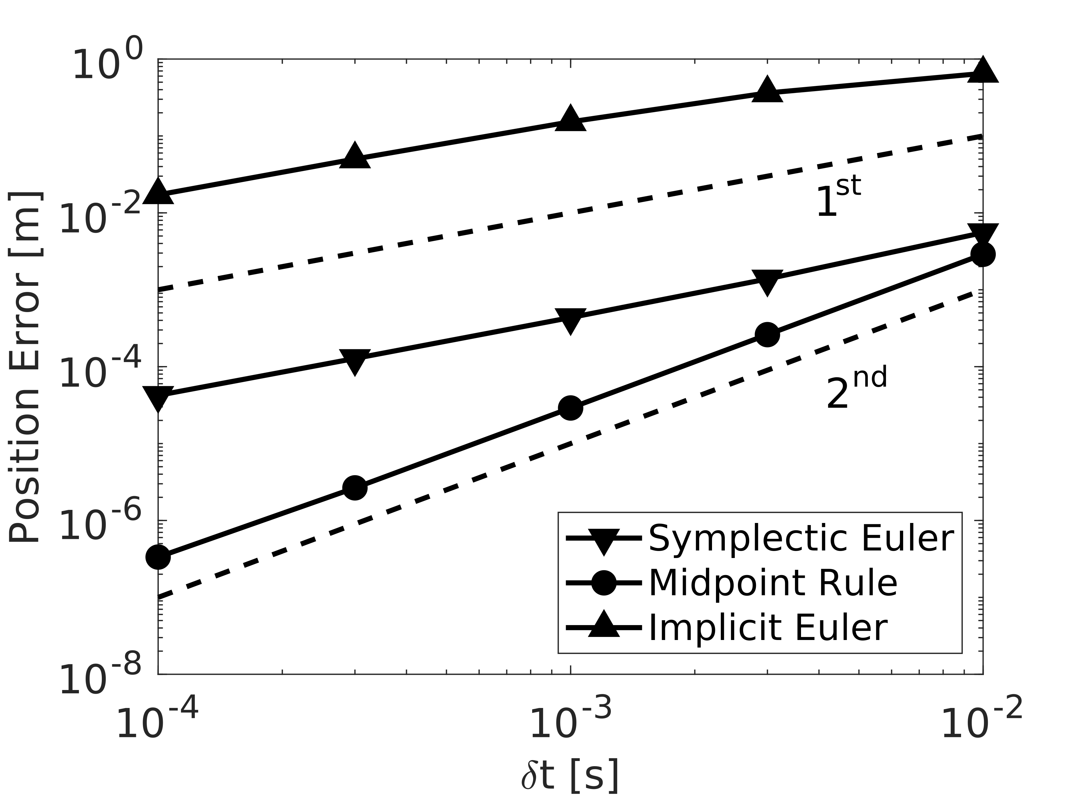
Figure 7: Position error as a function of time step for the spring-cylinder system with friction. First and second order references are shown with dashed lines.

VI-C Clutter

Objects are dropped into an $80~{}\text{cm}\times 80~{}\text{cm}\times 80~{}\text{cm}$ container in four different columns with the same number of objects in each (see Fig. 8). Each column consists of an arbitrary assortment of spheres of radius $5~{}\text{cm}$ and boxes with sides of $10~{}\text{cm}$ in length. With a density of $1000\text{kg}/\text{m}^{3}$, spheres have a mass of $0.524\text{ kg}$ and boxes have a mass of $1.0\text{ kg}$. We set a very high contact stiffness of $k=10^{12}\text{ N}/\text{m}$ so that the model is in the near-rigid regime. The dissipation time scale is set to equal the time step and the friction coefficient of all surfaces is $\mu=1.0$.

Figure 8: Initial conditions (top) and an intermediate configuration after $2$ seconds of simulated time (bottom) for the clutter setup with (left) and without (right) walls. Many of the spheres in the configuration with no walls roll outside the frame in the intermediate configuration.

We first run our simulations with 10 bodies per column for a total of 40 bodies. We simulate 10 seconds using time steps of size $\delta t=10\text{ ms}$. Number of solver iterations and wall-clock time per time step are reported in Fig. 9. We observe that SAP needs to perform a larger number of iterations during the very energetic initial transient. As the system reaches a steady state, however, SAP warm starts very effectively, performing only about $3$ iterations per time step. Even though SAP necessities a larger number of iterations to converge than Geodesic IPM during this initial transient, the wall-clock time per time step is very similar. Unlike SAP and Geodesic IPM that benefit from warm start, Gurobi performs about $9$ iterations per time step in both the initial transient and the steady state.

Figure 9: Iterations and wall-clock time per time step for the clutter case with 40 bodies and with walls.

Figure 10 shows two examples of convergence history. We denote with $\ell^{0}$ the cost evaluated at the initial guess, the previous time step velocity. With $\ell_{*}$ we denote the optimal cost, which we approximate with its value from the last iteration. At step 60 during the initial transient for which SAP requires 21 iterations to converge, we observe that the algorithm reaches quadratic convergence after an initial linear convergence transient, matching theoretical predictions (Appendix E). At step 520, past the initial energetic transient, SAP exhibits linear convergence and satisfies the convergence criteria within 5 iterations.

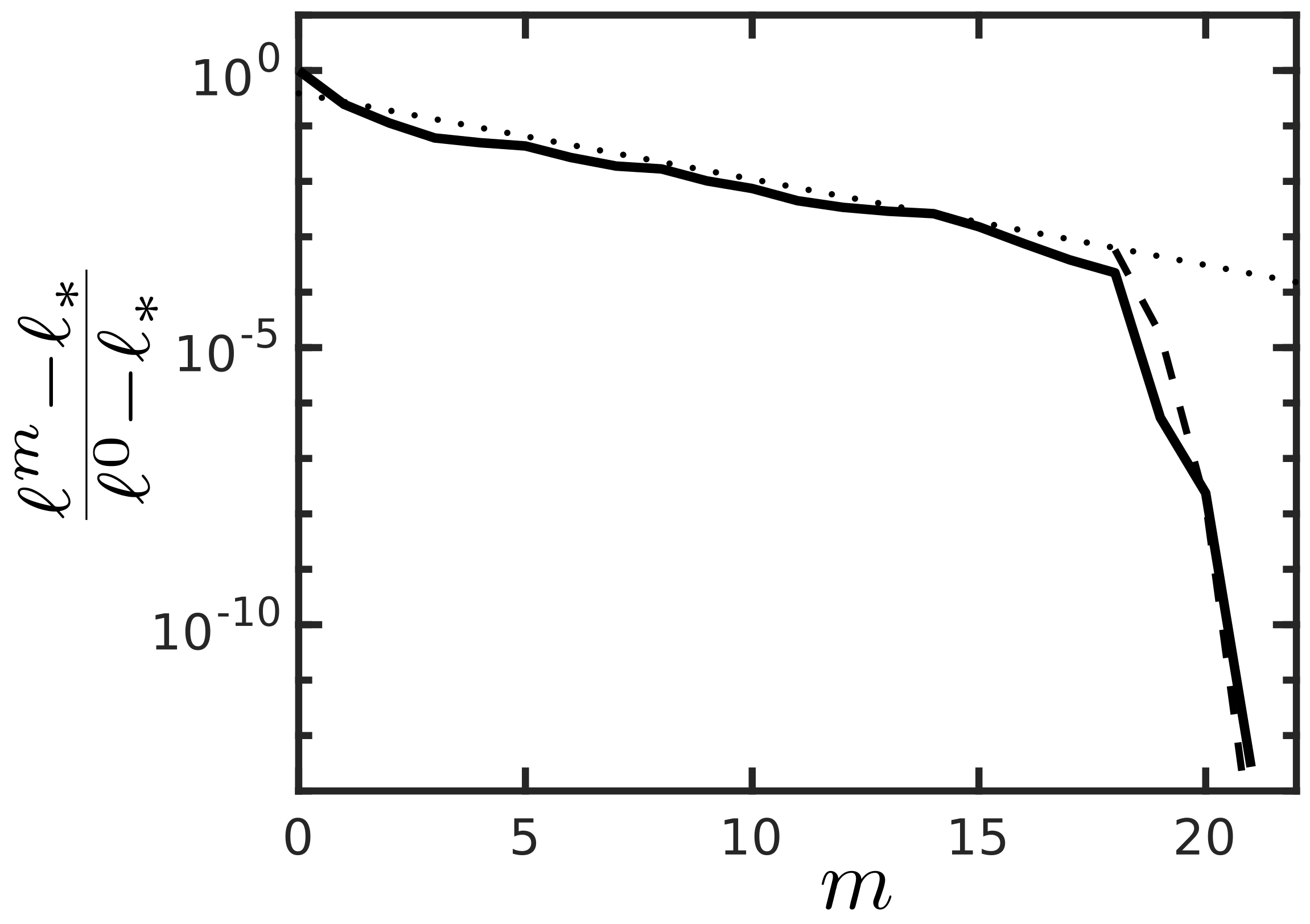
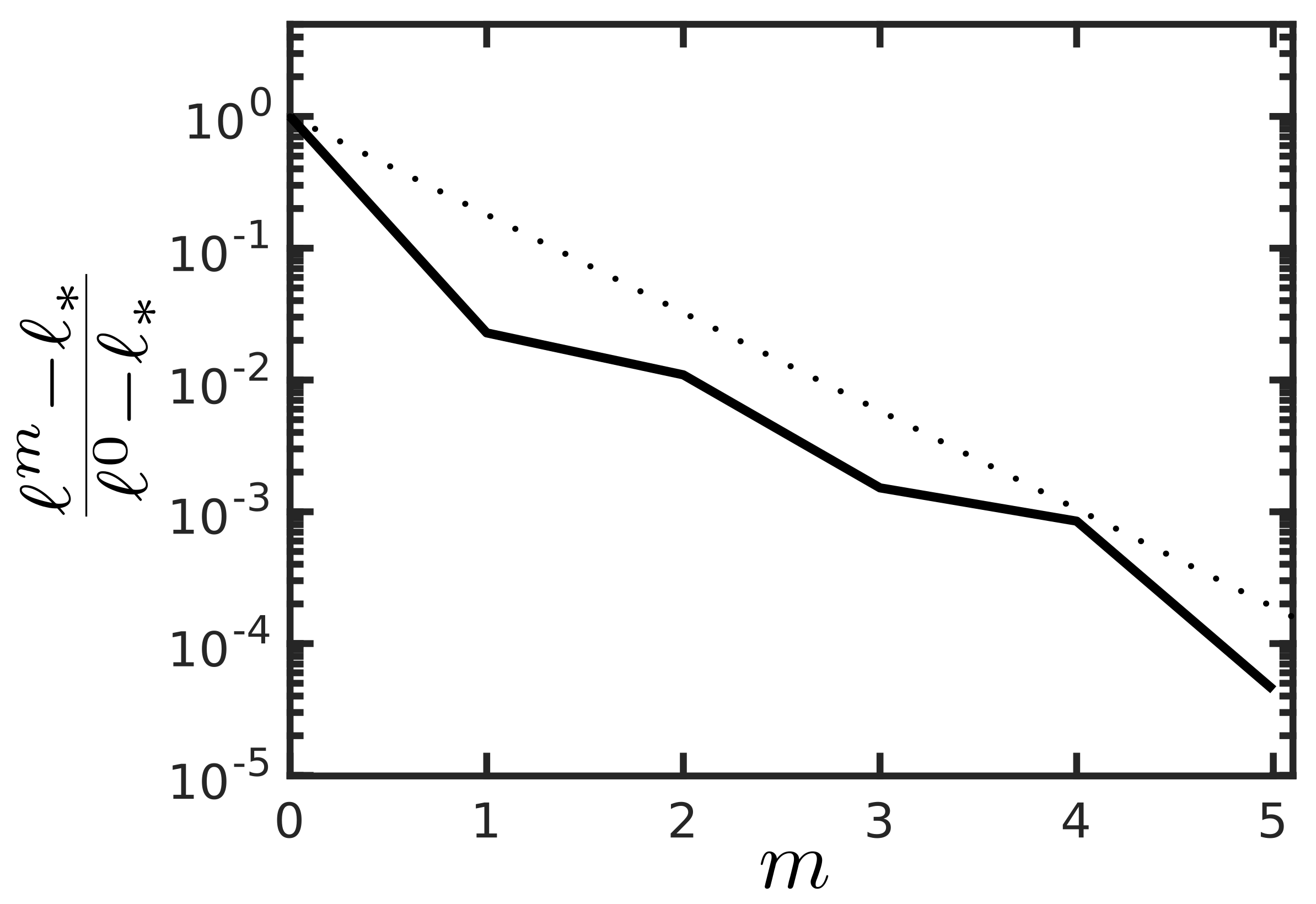
Figure 10: Cost as a function of Newton iterations for step 60 (left) and for step 520 (right) using SAP. The cost decreases monotonically. Reference lines are shown for linear convergence (dotted) and quadratic convergence (dashed).

VI-C1 Scalability

We evaluate the scalability of SAP by varying the number of objects in the clutter. We study the case with and without walls (see Fig. 8) as this variation leads to very different contact configurations and sparsity patterns. The size of the problems can be appreciated in Fig. 11 showing the number of contact constraints at the end of the simulation when objects are in steady state. We observe a larger number of contacts for the configuration without walls since in this configuration many of the boxes spread over the ground and lay flat on one of their faces, leading to multi-contact configurations (see Fig. 8).

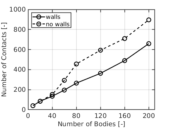
Figure 11: Total number of contacts with objects in steady state at the end of the simulation for setups with and without walls.

We define the speedup against Gurobi as the ratio of the wall-clock time spent by a solver to the wall-clock time reported by Gurobi. Figure 12 shows the speedup for both SAP and Geodesic IPM in the configuration with and without walls. The setup with walls is particularly difficult given that objects are constrained to pile up, leading to a configuration in which almost all objects are coupled with every other object by frictional contact (see Fig. 8). For example, the motion of an object at the bottom of the pile can lead to motion of another object far on top of the pile. In contrast, the simulation with no walls leads to islands of objects that do not interact with each other.

In general, we observe two regimes. For problems with less than about 40 bodies, SAP outperforms Gurobi significantly by up to a factor of 25 in the case with walls and up to a factor of 50 with no walls. Beyond 80 bodies, Gurobi outperforms both SAP and Geodesic IPM in the case with walls, but SAP is about 10 times faster for the case with no walls. Though SAP shows to be about twice as fast as Geodesic IPM for most problem sizes, it can be five times faster for small problems with 8 bodies or less.

Figure 12: Speedup against Gurobi for the configuration with walls (left) and without walls (right).

It could be argued that these speedup results depend on the accuracy settings of each solver. For a fair comparison, we define the dimensionless momentum error as

$$e_{m}=\frac{\|\tilde{\nabla}\ell_{p}\|}{\max(\|\tilde{{\mathbf{p}}}\|,\|\tilde{{\mathbf{j}}_{c}}\|)},$$ (32)

using the scaled generalized momentum quantities in Eq. (25). We also define the dimensionless complementarity slackness error as

$$e_{\mu}=\frac{1/n_{c}\sum_{i}|\bm{g}_{i}\cdot{\bm{\gamma}}_{i}|}{\ell_{p}}.$$ (33)

Figure 13 shows average values of $e_{m}$ and $e_{\mu}$ over all time steps. Since SAP satisfies the complementarity slackness exactly, $e_{\mu}$ is not shown. We have verified this to be true within machine precision for all simulated cases.

SAP’s momentum error is below $10^{-5}$ as expected since this is the value used for the termination condition. Similarly, the complementarity slackness is below $10^{-5}$ for Geodesic IPM, since this is the value used for its own termination condition. Gurobi does a good job at satisfying the complementarity slackness. However, it is the solver with the largest error in the momentum equations, even though both SAP and Geodesic IPM outperform Gurobi in most of the test cases. These metrics demonstrate that when SAP and Geodesic IPM outperform Gurobi, it is not at the expense of accuracy.

Figure 13: Momentum balance error $e_{m}$ (top) and complementarity condition error $e_{\mu}$ (bottom) for the clutter case with walls (left) and without walls (right).

VI-C2 Slip Parameter

We study the effect of the slip parameter $\sigma$ in Eq. (30). We use $\delta t=10\text{ ms}$ and simulate with SAP 40 objects for 10 seconds to a steady state configuration. At this steady state, we compute the mean slip velocity among all contacts, shown in Fig. 14 along with the estimated slip in Eq. (31), $v_{s}\approx\sigma\mu\delta tg$. We see that the mean slip velocity remains below the estimated slip as expected in a static configuration with objects in stiction. In the case with walls where stiction helps to hold the steady state static configuration, we see that the mean slip velocity closely follows the slope of the slip estimate. Without the walls, objects do not pile up in a complex static structure but simply lie on the ground, and therefore, the resulting slip velocities are significantly smaller. The sudden drop in the slip velocity for $\sigma>10^{-3}$ is caused by the sensitivity of the final state on the value of $\sigma$. As $\sigma$ increases, so does the slip velocity bound $v_{s}$ and objects in the configuration without walls can slowly drift into a configuration leading to more contacts. In particular, boxes are more likely to slowly drift until one of their faces lies flat on the ground, a configuration with zero slip once steady state is reached.

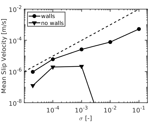
Figure 14: Mean slip velocity at the end of the simulation with objects at rest as a function of the slip parameter. The estimated bound $v_{s}=\sigma\mu\delta tg$ is shown in dashed lines.

We conclude by examining the effect of $\sigma$ on the conditioning of the system. Figure 15 shows the condition number of the Hessian in the final configuration and the mean number of Newton iterations throughout the simulation. We see that the condition number scales as $\sigma^{-1}$ while the mean number of Newton iterations is roughly proportional to $\ln(\sigma)$. Our default choice $\sigma=10^{-3}$ is a good compromise between accurate stiction, performance and conditioning.

Figure 15: Effect of the slip parameter on the mean Newton iterations per step (left) and mean condition number (right).

VI-D Slip Control

While previous work on convex approximations model rigid contact [14, 15] or use regularization as a means of constraint stabilization [17], our work is novel in that we incorporate physical compliance. This allows us not only to model compliant point contact, but also to incorporate sophisticated models of surfaces patches. We incorporate the pressure field model [35] implemented as part of Drake’s [24] hydroelastic contact model. We use the discrete approximation introduced in [36] to approximate each face of the contact surface as a compliant contact point at its centroid.

To demonstrate this capability, we reproduce the test in [36] that models a Soft-bubble gripper [51]; a parallel jaw WSG 50 Schunk gripper outfitted with air filled compliant surfaces (Fig. 16). The aforementioned gripper is simulated anchored to the world holding a spatula by the handle horizontally. We use $\delta t=5\times 10^{-3}\text{ s}$. The grasp force is commanded to vary between 1 N and 16 N with square wave having a 6 second period and a 75% duty cycle (see Fig. 17, left). This results in a periodic transition from a secure grip to a loose grip allowing the spatula to pitch in a controlled manner within grasp (see Fig. 17 and the accompanying video). These contact mode transitions are resolved by our model. We observe that stiction during the secure grip is properly resolved with the tight bounds for the slip due to regularization discussed in Section V-B. While this case only has 8 degrees of freedom, it generates about 60 contact constraints during the slip phase and about 160 contact constraints during the stiction phase.

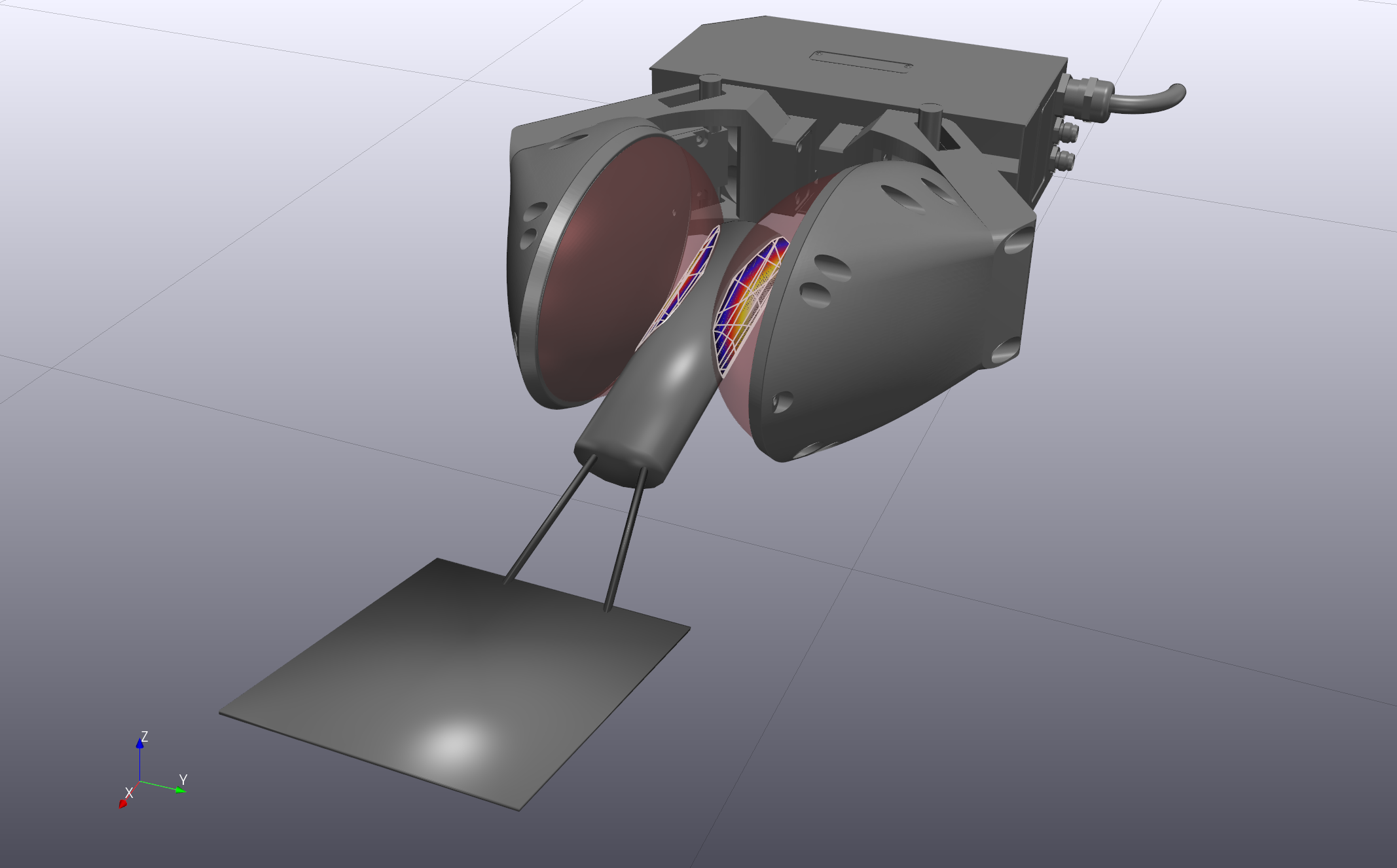
Figure 16: Highly compliant Soft-bubble gripper [51] holding a spatula. Unlike traditional point contact approaches, the hydroelastic contact model provides rich contact information and captures area-dependent phenomena such as the net-torque to hold the spatula. Contact patches are colored by contact pressure.

Figure 17: Grip force command (left) and spatula pitch angle (right) as a function of time.

We compare the performance of SAP against both Gurobi and Geodesic IPM, see Section VI-A. For SAP we use a relative tolerance $\varepsilon_{r}=10^{-3}$, see Section IV-E. For Gurobi we set its tolerance parameter BarQCPConvTol to $10^{-8}$. For Geodesic IPM, we set its complementary slackness tolerance to $10^{-6}$; larger values lead to failure for this task. SAP bounds the momentum error, exhibiting a maximum value of of $9.99\times 10^{-2}\,\%$. Even with such a tight tolerance, Gurobi exhibits $2.6\,\%$ maximum error. Geodesic IPM’s errors are significantly smaller, below $2\times 10^{-4}\,\%$. However its robustness is very sensitive to the specified tolerance.

Even though SAP’s solutions are significantly more accurate than those from Gurobi, it performs 92 times faster than Gurobi. SAP is 20 times faster than Geodesic IPM and significantly more robust to solver tolerances. In terms of solver iterations, SAP only performs 0.62 iterations on average, showcasing how effectively it warm-starts. Geodesic IPM performs 5.6 iterations per step on average and Gurobi performs 10.1 iterations on average.

VI-E Dual Arm Manipulation

We demonstrate the effectiveness of our approach with the simulation of a complex manipulation task. In this scenario, two Kuka IIWA arms (7 DOFs each) are outfitted with anthropomorphic Allegro hands (16 DOFs each) (Fig. 1). In front of the robot, a table has a jar (with a lid, 12 DOFs) full of 16 marbles of $50$ gr each (96 DOFs) and a bowl (6 DOFs), completing the model with a total of 160 DOFs. Contact between the jar and the lid is modeled using Drake’s hydroelastic model [35, 36] (see Section VI-D), while point contact is used for all other interactions. The time step is set to $\delta t=5\times 10^{-3}$ s.

The arms’ controllers track a prescribed sequence of Cartesian end-effector keyframe poses, while the hands’ controllers track prescribed open/close configurations. We use force feedback to gauge successful grasps and to know when the jar makes contact with the table. The robot is commanded to open the jar, pour its contents into the bowl, close the lid and put the empty jar back in place (keyframes in Fig. 1 and the accompanying video).

This particular task generates hundreds of contact constraints, as shown in Fig. 18 which also labels important events during the task. We remark that our framework predicts contact mode switching as a result of the computation. For instance, the lid initially covering the jar is held by stiction and it transitions to sliding as the robot pulls it out.

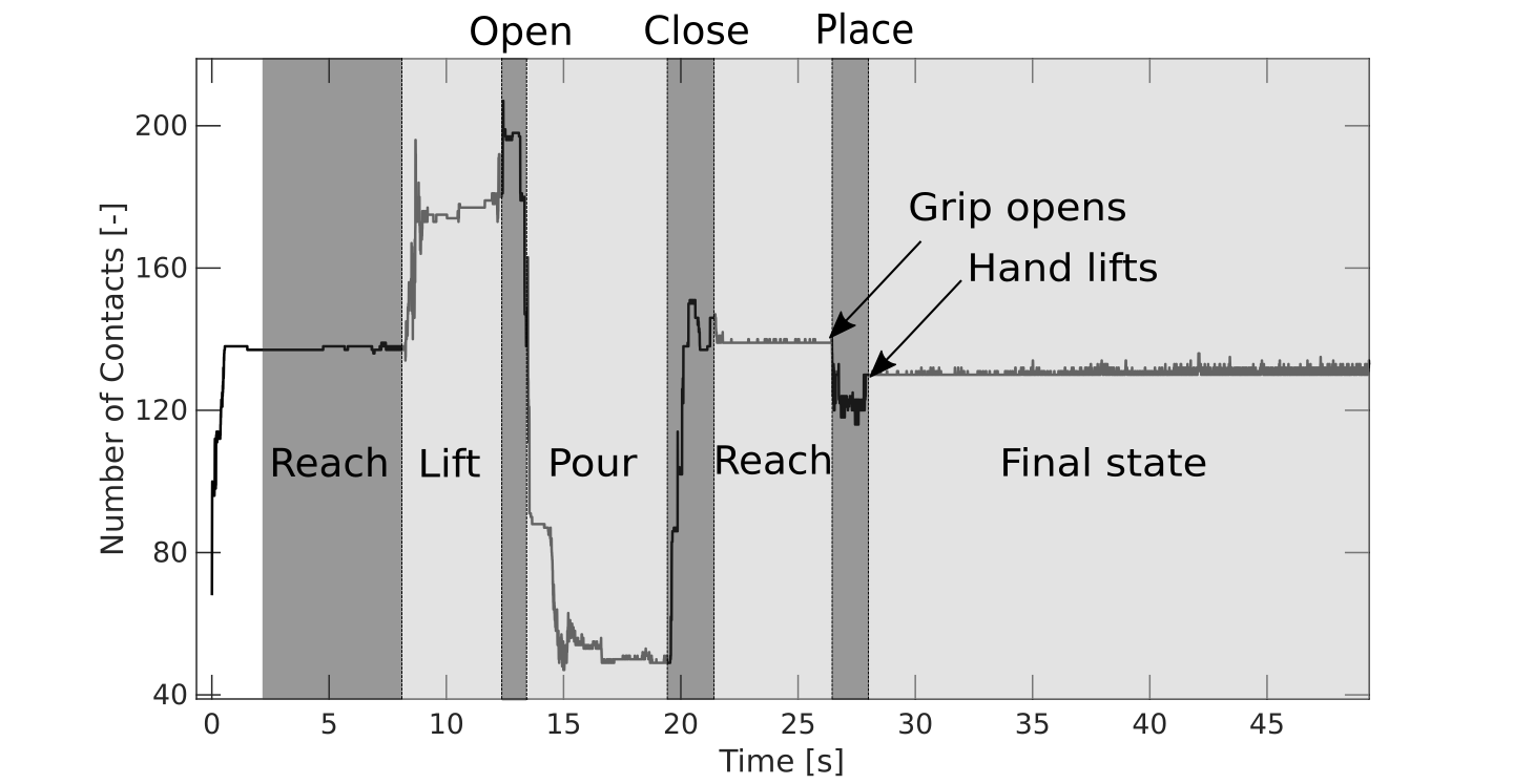
Figure 18: Number of contact constraints as a function time. Important events during the task are highlighted.

To assess accuracy, we evaluate the dimensionless momentum and complementarity slackness errors defined in Eqs. (32) and (33) respectively. We perform the simulation of the same task several times using different solver tolerances. The results of these runs are shown in Figures 19 and 20. Even though each solver uses a different tolerance parameter, it is still useful to place these tolerances in the same horizontal axis. The maximum tolerance we use for each solver corresponds to the largest value that can be used to complete the task successfully. For Gurobi and Geodesic IPM, smaller values of the tolerance parameter make the simulation impractically slow. SAP on the other hand cannot achieve errors below $10^{-6}$ for this case due to round-off errors. Figures 19 and 20 show both mean and median of the errors over the entire simulation to show errors do not follow a symmetric distribution. More interesting however are the minimum and maximum errors, shown as shaded areas. SAP guarantees that momentum errors are below the specified tolerance, given this is precisely its stopping criteria in Eq. (26). We see however that it is difficult to correlate the expected error to solver tolerance when using Gurobi or Geodesic IPM. In practice, we consistently observe that the robot does not complete the task successfully when momentum errors are larger than about $10\%$, regardless of the solver. Therefore, we find that being able to specify a tolerance for the momentum error directly is immensely useful. Given that SAP satisfies the complementarity slackness condition exactly, complementarity slackness error for SAP is not included in Fig. 20.

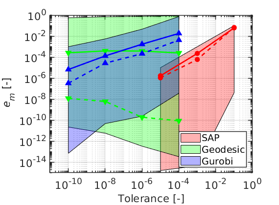
Figure 19: Dimensionless momentum error, defined in Eq. (32). Mean (solid) and median (dashed) errors along with minimum and maximum errors (shaded areas) over the entire simulation.

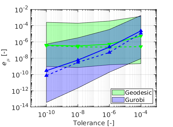
Figure 20: Dimensionless complementarity slackness error, defined in Eq. (33). Mean (solid) and median (dashed) errors along with minimum and maximum errors (shaded areas) over the entire simulation.

Figure 21 shows the mean number of iterations per time-step for each solver. We see that the number of iterations needed by the SAP solver is consistently below the other two solvers given how effectively SAP warm-starts from the previous time-step solution.

To make a fair comparison among solvers, from Fig. 19 we choose tolerances for each solver that result in similar values of the mean momentum error. For Gurobi, we set its tolerance parameter BarQCPConvTol to $10^{-8}$. For Geodesic IPM, we set its complementary slackness tolerance to $10^{-6}$. For SAP, we set its relative tolerance to $10^{-3}$. Notice this is not entirely fair to SAP, given that SAP does guarantee the maximum momentum error to be below $10^{-3}$, while this is not true for the other two solvers. Still, SAP is 7.4 faster than Gurobi and 2.2 faster than Geodesic IPM. In terms of iterations, SAP performs 4 iterations on average while Geodesic IPM performs 8.3 iterations on average. This shows that since both solvers use exactly the same sparse algebra, the performance gains with SAP are entirely due to its ability to warm-start effectively rather than to differences in the implementation. The general purpose solver Gurobi on the other hand performs 10.1 iterations on average.

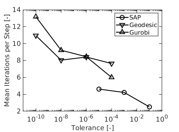
Figure 21: Mean number of iterations per time-step for the dual arm simulation.

In summary, the simulation of this complex robotic task demonstrates how accuracy translates directly to robustness. We observe how the maximum momentum error defined in Eq. (32) is a good proxy for robustness in simulation; simulations with errors larger than about $10\%$ could not complete the task successfully. In this regard, SAP provides a certificate of accuracy that proves useful in practice.

VII Variations and Extensions

The method presented in this paper can be extended in several ways:

Expand the family of constraints: No doubt contact constraints are the most challenging. However, our method can be extended to include bilateral constraints, PD controllers with force limits and even joint dry friction [17].

Branch induced sparsity: In this work we exploit sparsity only at the tree level. However, branch sparsity can lead to additional performance. Consider for instance a standing humanoid robot with a floating hip. Since arms and the upper torso are not in contact with the ground, they can be eliminated from the computation. Additional performance gains could be attained using specialized algebra for multibody dynamics [52].

Parallelization: This work focuses on accuracy, robustness, and convergence properties of the algorithm executed in a single thread. The sparse algebra can be parallelized and, in particular, disjoint islands of bodies can be solved separately in different threads.

Deformable FEM models: Using the SAP solver for the modeling of deformable objects with contact and friction is the topic of current research efforts by the authors. FEM models lead to state dependent stiffness (16) and damping (17) matrices with a complex structure that requires specialized handling of sparsity. Moreover, modeling assumptions must be carefully analyzed in order to ensure the positive definiteness of these matrices used in our convex approximation of contact.

Differentiation: Since forces are a continuous function of state, the model is well suited for applications requiring gradients such as trajectory optimization, machine learning, parameter estimation, and control. Factorizations computed during forward dynamics can be reused when computing gradients for a performant implementation.

VIII Limitations

All models are approximations of reality, while numerical methods can only approximate our models. We list here the limitations we identify for our method.

Convex Approximation: The convex approximation amounts to a gliding effect during sliding at a distance $\phi\sim\delta t\mu\|{\bm{v}}_{t}\|$. Regularization leads to a model of regularized friction, Eq. (28). Details are provided in Section V.

Stiffness and Dissipation: Our method requires stiffness ${\mathbf{K}}$ and damping ${\mathbf{D}}$ matrices to be SPD or SPD approximations (see Section II-D). For joint level spring-dampers, the exact ${\mathbf{K}}$ and ${\mathbf{D}}$ can be used, but for other forces such as those arising from a spatial arrangement of springs, an SPD approximation must be made as ${\mathbf{K}}$ might not be SPD in certain configurations.

Linear Approximations: Algorithm 1 evaluates the SPD gradient ${\mathbf{A}}$ once at ${\mathbf{v}}^{*}$ at each time step. In other words, our method replaces the original balance of momentum (7) with its linear approximation (18). This is exact for many important cases and accurate to second-order in the general case. See Section III-C for details.

Delassus Operator Estimation: In Section V-B we use a diagonal approximation of the Delassus operator to estimate stiffness in the near-rigid regime. Corner cases exist. Consider a pile of books. While the inertia of a contact at the bottom of the pile is estimated solely on the mass of one book, this contact is supporting the weight of the entire stack. Stiffness is underestimated and user intervention is needed to set proper parameters.

Scalability: We see no reason SAP with the direct supernodal algebra (Section IV-D) could not scale to thousands of bodies if there is structured sparsity. However, scalability needs to be studied further, along with the usage of iterative solvers such as Conjugate Gradient (CG), widely used in optimization.

IX Conclusion

We presented a novel unconstrained convex formulation of compliant contact. In this formulation constraints are eliminated using analytic formulae that we developed. Our scheme incorporates the midpoint rule into a two-stage scheme, with demonstrated second order accuracy. We rigorously characterized our numerical approximations and the artifacts introduced by the convex approximation of contact. We reported limitations of our method and discussed extensions and areas of further research.

We showed that regularization maps to physical compliance, allowing us to eliminate algorithmic parameters and to incorporate complex models of continuous contact patches. Moreover, we studied the trade off between regularization and numerical conditioning for the simulation of near-rigid bodies and the accurate resolution of stiction.

We presented SAP, a robust and performant solver that warm-starts very effectively in practice. SAP globally converges at least at a linear-rate and exhibits quadratic convergence when additional smoothness conditions are satisfied. SAP can be up to 50 times faster than Gurobi in small problems with up to a dozen objects and up to 10 times faster in medium sized problems with about 100 objects. Even though SAP uses the supernodal algebra implemented for Geodesic IPM, it performs at least two times faster due to its effective warm-starts from the previous time-step solution. Moreover, SAP is significantly more robust in practice given that it guarantees a hard bound on the error in momentum, effectively providing a certificate of accuracy.

We have incorporated SAP into the open source robotics toolkit Drake [24], and hope that the simulation and robotics communities can benefit from our contribution.

Appendix A Proof of Proposition 1

The Taylor expansion of ${\mathbf{m}}({\mathbf{v}})$ at ${\mathbf{v}}={\mathbf{v}}^{*}$ reads

$${\mathbf{m}}({\mathbf{v}}) ={\mathbf{m}}^{*}+\frac{\partial{\mathbf{m}}}{\partial{\mathbf{v}}}({\mathbf{v}}-{\mathbf{v}}^{*})+\mathcal{O}_{m}(\|{\mathbf{v}}-{\mathbf{v}}^{*}\|^{2})$$

$$=\frac{\partial{\mathbf{m}}}{\partial{\mathbf{v}}}({\mathbf{v}}-{\mathbf{v}}^{*})+\mathcal{O}_{m}(\|{\mathbf{v}}-{\mathbf{v}}^{*}\|^{2}),$$ (34)

where we use the fact that by definition ${\mathbf{m}}^{*}={\mathbf{m}}({\mathbf{v}}^{*})={\mathbf{0}}$. All derivatives are evaluated at ${\mathbf{v}}={\mathbf{v}}^{*}$ unless otherwise noted. We first evaluate the Jacobian of the mass matrix term in Eq. (14)

$$\frac{\partial\left({\mathbf{M}}({\mathbf{q}}^{\theta}({\mathbf{v}}))({\mathbf{v}}-{\mathbf{v}}_{0})\right)}{\partial{\mathbf{v}}}={\mathbf{M}}({\mathbf{q}}^{\theta}({\mathbf{v}}^{*}))+{\mathbf{E}},$$

where we defined

$${\mathbf{E}}=\frac{\partial{\mathbf{M}}({\mathbf{q}}^{\theta})}{\partial{\mathbf{v}}}({\mathbf{v}}^{*}-{\mathbf{v}}_{0}).$$

Note that by combining Eqs. (6) and (12), the mid-step configuration ${\mathbf{q}}^{\theta}$ can be written as

$${\mathbf{q}}^{\theta}({\mathbf{v}}) ={\mathbf{q}}_{0}+\delta t\theta\dot{{\mathbf{q}}}^{\theta_{vq}}$$

$$={\mathbf{q}}_{0}+\delta t\theta{\mathbf{N}}({\mathbf{q}}^{\theta}){\mathbf{v}}^{\theta_{vq}}({\mathbf{v}}).$$

Hence by the chain rule, ${\mathbf{E}}$ can be further calculated as

$${\mathbf{E}}=\delta t\theta\frac{\partial{\mathbf{M}}({\mathbf{q}}^{\theta})}{\partial{\mathbf{q}}}\frac{\partial\dot{{\mathbf{q}}}^{\theta_{vq}}}{\partial{\mathbf{v}}}({\mathbf{v}}^{*}-{\mathbf{v}}_{0}).$$

Notice that

$$\|{\mathbf{E}}\| \leq\delta t\theta\left\|\frac{\partial{\mathbf{M}}({\mathbf{q}}^{\theta})}{\partial{\mathbf{q}}}\right\|\left\|\frac{\partial\dot{{\mathbf{q}}}^{\theta_{vq}}}{\partial{\mathbf{v}}}\right\|\left\|{\mathbf{v}}^{*}-{\mathbf{v}}_{0}\right\|$$

$$=\mathcal{O}(\delta t^{2}),$$

since $\|{\mathbf{v}}^{*}-{\mathbf{v}}_{0}\|=\mathcal{O}(\delta t)$.

We proceed similarly to expand the Jacobian of ${\mathbf{F}}_{1}({\mathbf{v}})={\mathbf{F}}_{1}({\mathbf{q}}^{\theta}({\mathbf{v}}),{\mathbf{v}}^{\theta}({\mathbf{v}}))$ as

$$\frac{\partial{\mathbf{F}}_{1}}{\partial{\mathbf{v}}}=-\delta t\,\theta\theta_{vq}{\mathbf{K}}({\mathbf{q}}^{\theta},{\mathbf{v}}^{\theta})-\theta{\mathbf{D}}({\mathbf{q}}^{\theta},{\mathbf{v}}^{\theta}),$$

with ${\mathbf{K}}$ and ${\mathbf{D}}$ the stiffness and damping matrices defined by Eqs. (16)-(17).

We can now write the Jacobian of ${\mathbf{m}}({\mathbf{v}})$ in Eq. (34) as

$$\frac{\partial{\mathbf{m}}}{\partial{\mathbf{v}}}={\mathbf{A}}+{\mathbf{E}}-\delta t\frac{\partial{\mathbf{F}}_{2}}{\partial{\mathbf{v}}},$$

where we defined

$${\mathbf{A}}={\mathbf{M}}+\delta t^{2}\theta\theta_{qv}{\mathbf{K}}+\delta t\theta{\mathbf{D}}.$$

With these definitions the Taylor expansion in Eq. (34) becomes

$$\frac{\partial{\mathbf{m}}}{\partial{\mathbf{v}}}({\mathbf{v}}-{\mathbf{v}}^{*}) ={\mathbf{A}}({\mathbf{v}}-{\mathbf{v}}^{*})+{\mathbf{E}}({\mathbf{v}}-{\mathbf{v}}^{*})$$

$$-\delta t\frac{\partial{\mathbf{F}}_{2}}{\partial{\mathbf{v}}}({\mathbf{v}}-{\mathbf{v}}^{*})+\mathcal{O}_{m}(\|{\mathbf{v}}-{\mathbf{v}}^{*}\|^{2}).$$

Since contact is compliant, forces are finite within the finite interval $\delta t$ and therefore $\|{\mathbf{v}}-{\mathbf{v}}^{*}\|=\mathcal{O}(\delta t)$. Thus

$${\mathbf{E}}({\mathbf{v}}-{\mathbf{v}}^{*})=\mathcal{O}_{E}(\delta t^{3}),$$

$$\delta t\frac{\partial{\mathbf{F}}_{2}}{\partial{\mathbf{v}}}({\mathbf{v}}-{\mathbf{v}}^{*})=\mathcal{O}_{F_{2}}(\delta t^{2}),$$

$$\mathcal{O}_{m}(\|{\mathbf{v}}-{\mathbf{v}}^{*}\|^{2})=\mathcal{O}_{m}(\delta t^{2}).$$

Therefore, the positive definite linearization

$${\mathbf{A}}({\mathbf{v}}-{\mathbf{v}}^{*})+\mathcal{O}_{E}(\delta t^{3})+\mathcal{O}_{F_{2}}(\delta t^{2})+\mathcal{O}_{m}(\delta t^{2})={\mathbf{J}}^{T}{\mathbf{{\bm{\gamma}}}},$$

agrees with the original momentum balance in Eq. (7) to second order.

Finally, notice that ${\mathbf{A}}$ is a linear combination of positive definite matrices with non-negative scalars in the linear combination, and therefore ${\mathbf{A}}\succ 0$. ∎

Appendix B Proof of Theorem 2

Before proving this theorem, we need the following result.

Lemma 1.

The conic constraint ${\mathbf{g}}({\mathbf{v}},{\bm{\sigma}})\in\mathcal{F}^{*}$ is satisfied if ${\bm{\sigma}}$ is given by $P_{\mathcal{F}}({\mathbf{y({\mathbf{v}})}})$.

Proof:

Since ${\bm{\sigma}}$ is the projection of ${\mathbf{y}}({\mathbf{v}})$ to the cone $\mathcal{F}$ with the ${\mathbf{R}}$ norm, by Moreau’s decomposition theorem, we know that ${\mathbf{y}}({\mathbf{v}})-{\bm{\sigma}}$ is in the polar cone of $\mathcal{F}$ with the ${\mathbf{R}}$ norm. That is, $\langle{\mathbf{y}}({\mathbf{v}})-{\bm{\sigma}},{\mathbf{x}}\rangle_{\mathbf{R}}\leq 0$ for all ${\mathbf{x}}\in\mathcal{F}$, with the inner product $\langle{\mathbf{v}},{\mathbf{w}}\rangle_{\mathbf{R}}={\mathbf{v}}^{T}{\mathbf{R}}{\mathbf{w}}$. Reorganizing terms, we get

$${\mathbf{x}}^{T}{\mathbf{R}}({\mathbf{y}}({\mathbf{v}})-{\bm{\sigma}}) \leq 0,$$

$${\mathbf{x}}^{T}(-{\mathbf{R}}{\bm{\sigma}}-{\mathbf{v}}_{c}+\hat{{\mathbf{v}}}_{c}) \leq 0,$$

$$\langle{\mathbf{x}},-{\mathbf{R}}{\bm{\sigma}}-{\mathbf{v}}_{c}+\hat{{\mathbf{v}}}_{c}\rangle \leq 0,$$

for all ${\mathbf{x}}\in\mathcal{F}$. Therefore, it follows that $-{\mathbf{g}}=-({\mathbf{v}}_{c}-\hat{{\mathbf{v}}}_{c}+{\mathbf{R}}{\bm{\sigma}})$ is in the polar cone of $\mathcal{F}$ and thus ${\mathbf{g}}$ is in the dual cone of $\mathcal{F}$. ∎

The optimality condition for the unconstrained formulation in (24) is $\nabla\ell_{p}({\mathbf{v}})={\mathbf{0}}$. It is shown in Appendix D that

$$\nabla\ell_{p}({\mathbf{v}})={\mathbf{A}}({\mathbf{v}}-{\mathbf{v}}^{*})-{\mathbf{J}}^{T}{\bm{\gamma}}({\mathbf{v}}),$$

with impulses given by ${\bm{\gamma}}({\mathbf{v}})=P_{\mathcal{F}}({\mathbf{y}}({\mathbf{v}}))$, the dual optimal. Therefore, $\nabla\ell_{p}({\mathbf{v}})={\mathbf{0}}$ implies (21a), the first optimality condition for (19).

The analytical inverse dynamics solution shows that ${\bm{\gamma}}=P_{\mathcal{F}}({\mathbf{y({\mathbf{v}})}})$ with the primal optimal ${\mathbf{v}}$. Hence, choosing ${\bm{\sigma}}=P_{\mathcal{F}}({\mathbf{y({\mathbf{v}})}})$ with the primal optimal ${\mathbf{v}}$ satisfies (21b), the second optimality condition for (19).

Finally, by Lemma 1, the cone constraint ${\mathbf{g}}({\mathbf{v}},{\bm{\sigma}})\in\mathcal{F}^{*}$ is satisfied. ∎

Appendix C Analytical Inverse Dynamics

We perform the projection in Eq. (23) for a regularization of the form ${\bm{R}}=\text{diag}([R_{t},R_{t},R_{n}])$. For simplicity, we drop contact subindex $i$. We make the change of variables $\tilde{{\bm{\gamma}}}={\bm{R}}^{1/2}{\bm{\gamma}}$ and $\tilde{{\bm{y}}}={\bm{R}}^{1/2}{\bm{y}}$ [17], and observe that $\tilde{{\bm{\gamma}}}$ is the Euclidian projection of $\tilde{{\bm{y}}}$ onto cone $\tilde{\mathcal{F}}$ with coefficient $\tilde{\mu}=\mu\,(R_{t}/R_{n})^{1/2}$. We conclude that

$$P_{\mathcal{F}}({\bm{y}})={\bm{R}}^{-1/2}P_{\tilde{\mathcal{F}}}(\tilde{{\bm{y}}}),$$

We partition $\mathbb{R}^{3}$ into three regions, see Fig.  22: closed cone $\tilde{\mathcal{F}}$, denoted with $\mathcal{R}_{I}$, the interior of the polar $\tilde{\mathcal{F}}^{\circ}$, denoted with $\mathcal{R}_{III}$, and the remaining area, which we denote with $\mathcal{R}_{II}$. For $\tilde{{\bm{y}}}\in\mathcal{R}_{I}$ we simply have that $P_{\tilde{\mathcal{F}}}(\tilde{{\bm{y}}})=\tilde{{\bm{y}}}$. When $\tilde{{\bm{y}}}\in\mathcal{R}_{III}$, $P_{\tilde{\mathcal{F}}}(\tilde{{\bm{y}}})={\bm{0}}$. Finally, when $\tilde{{\bm{y}}}\in\mathcal{R}_{II}$, we evaluate $P_{\tilde{\mathcal{F}}}(\tilde{{\bm{y}}})$ via Euclidean projection onto the boundary of $\tilde{\mathcal{F}}$, which admits a simple formula. We define $\hat{{\bm{f}}}=[\tilde{\mu}\hat{{\bm{t}}},1]/\sqrt{1+\tilde{\mu}^{2}}$, the unit vector along the wall of the cone shown in Fig. 22, with $\hat{{\bm{t}}}=\tilde{{\bm{y}}}_{t}/\|\tilde{{\bm{y}}}_{t}\|={\bm{y}}_{t}/\|{\bm{y}}_{t}\|$. Then the projection is computed as $\tilde{{\bm{\gamma}}}=(\tilde{{\bm{y}}}\cdot\hat{{\bm{f}}})\hat{{\bm{f}}}$. After some algebraic manipulation we have that $P_{\tilde{\mathcal{F}}}(\tilde{{\bm{y}}})=[\tilde{{\bm{\gamma}}}_{t},\tilde{\gamma}_{n}]$ with

$$\tilde{{\bm{\gamma}}}_{t} =\tilde{\mu}\tilde{\gamma}_{n}\hat{{\bm{t}}},$$

$$\tilde{\gamma}_{n} =\frac{1}{1+\tilde{\mu}^{2}}\left(\tilde{y}_{n}+\tilde{\mu}\tilde{y}_{r}\right),$$

where $\tilde{y}_{r}=\|\tilde{{\bm{y}}}_{t}\|$. Note that this formula is well-defined on $\mathcal{R}_{II}$, since ${\bm{y}}_{t}={\bm{0}}$ only if ${\bm{y}}$ is in regions $\mathcal{R}_{I}$ or $\mathcal{R}_{III}$.

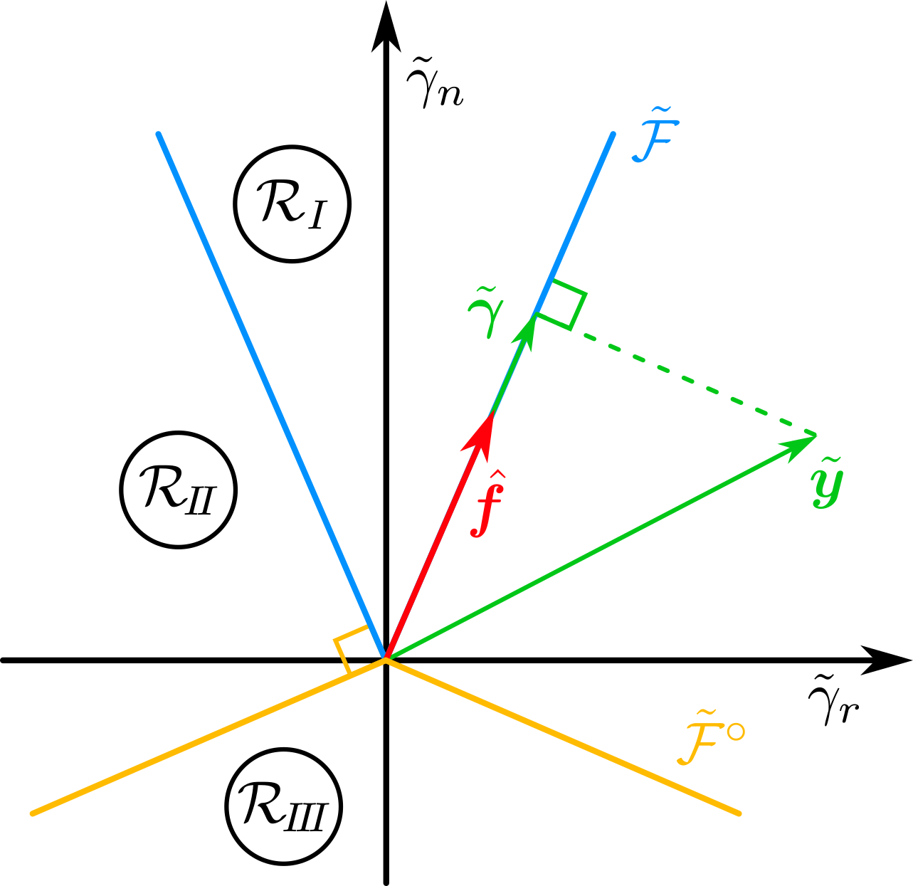
Figure 22: Geometry of the projection and regions in the $\tilde{{\bm{y}}}$ space.

Finally, we apply the inverse transformation ${\bm{\gamma}}={\mathbf{R}}^{-1/2}P_{\tilde{\mathcal{F}}}(\tilde{{\bm{y}}})$ and after some algebraic manipulation we recover the projection ${\bm{\gamma}}=P_{\mathcal{F}}({\bm{y}})$ in Eq. (V-A).

Appendix D Computation of the Gradients

We will start by taking derivatives of the regularizer term $\ell_{R}$. First we notice that we can write this term as

$$\ell_{R}=\frac{1}{2}\|{\bm{\gamma}}\|_{R}^{2}=\sum_{i}\ell_{R_{i}},$$

with $\ell_{R_{i}}=1/2\|{\bm{\gamma}}_{i}\|_{R_{i}}^{2}$. Since $\nabla_{{\bm{y}}_{j}}\ell_{R_{i}}={\bm{0}}$ for $i\neq j$, we only need to compute the gradients of $\ell_{R_{i}}({\mathbf{y}})$ with respect to the contact point variable ${\bm{y}}_{i}\in\mathbb{R}^{3}$. Dropping contact subindex $i$ for simplicity, we write the regularization as

$$\ell_{R}=\frac{1}{2}\|{\bm{\gamma}}\|_{R}^{2}=\frac{1}{2}(R_{t}\|{\bm{\gamma}}_{t}\|^{2}+R_{n}\gamma_{n}^{2}).$$

We use Eq. (V-A) to write the cost in terms of ${\bm{y}}$ as

$$\ell_{R}({\bm{y}})=$$ (35)

$$\begin{dcases}\frac{1}{2}(R_{t}y_{r}^{2}+R_{n}y_{n}^{2})&\text{stiction, }y_{r}\leq\mu y_{n}\\ \frac{R_{n}}{2(1+\tilde{\mu}^{2})}\left(y_{n}+\hat{\mu}y_{r}\right)^{2}&\text{sliding, }-\hat{\mu}y_{r}<y_{n}\leq\frac{y_{r}}{\mu}\\ {\bm{0}}&\text{no contact, }y_{n}<-\hat{\mu}y_{r}\end{dcases}$$

D-A Gradients per Contact Point

We use the following identities to simplify expressions

$$\frac{\partial y_{r}}{\partial{\bm{y}}_{t}}=\hat{{\bm{t}}},\quad\frac{\partial\hat{{\bm{t}}}}{\partial{\bm{y}}_{t}}=\frac{{\bm{P}}^{\perp}(\hat{{\bm{t}}})}{y_{r}},$$

where the $2\times 2$ projection matrix is

$${\bm{P}}^{\perp}(\hat{{\bm{t}}})={\bm{I}}_{2}-{\bm{P}}(\hat{{\bm{t}}}),\quad\text{with }{\bm{P}}(\hat{{\bm{t}}})=\hat{{\bm{t}}}\otimes\hat{{\bm{t}}}.$$

Taking the gradient of Eq. (35) results in

$$\nabla_{\bm{y}}\ell_{R}({\bm{y}})=$$ (36)

$$\begin{dcases}{\bm{R}}\,{\bm{y}}&\text{stiction, }y_{r}\leq\mu y_{n}\\ \frac{1}{1+\tilde{\mu}^{2}}\hat{s}^{\circ}({\bm{y}})\begin{bmatrix}\mu R_{t}\hat{{\bm{t}}}\\ R_{n}\\ \end{bmatrix}&\text{sliding, }-\hat{\mu}y_{r}<y_{n}\leq\frac{y_{r}}{\mu}\\ {\bm{0}}&\text{no contact, }y_{n}<-\hat{\mu}y_{r}\end{dcases}$$

with $\hat{s}^{\circ}({\bm{y}})=\hat{\mu}y_{r}+y_{n}$ positive in the sliding region. We note that $\nabla_{\bm{y}}\ell_{R}({\bm{y}})$ is not differentiable at the boundaries of $\mathcal{F}$ and $\mathcal{F}^{\circ}$. At points of differentiability, the Hessian $\nabla_{\bm{y}}^{2}\ell_{R}({\bm{y}})$ is computed by taking derivatives of Eq. (36)

$$\nabla_{\bm{y}}^{2}\ell_{R}({\bm{y}})=$$ (37)

$$\begin{dcases}{\bm{R}}&\text{stiction,}\\ \frac{R_{n}}{1+\tilde{\mu}^{2}}\begin{bmatrix}\hat{\mu}\left(\hat{\mu}{\bm{P}}(\hat{{\bm{t}}})+\hat{s}^{\circ}({\bm{y}}){\bm{P}}^{\perp}(\hat{{\bm{t}}})/y_{r}\right)&\hat{\mu}{\bm{t}}\\ \hat{\mu}{\bm{t}}^{T}&1\\ \end{bmatrix}&\text{sliding,}\\ {\bm{0}}&\text{no contact.}\end{dcases}$$

Clearly in the stiction region we have $\nabla_{\bm{y}}^{2}\ell_{R}({\bm{y}})\succ 0$. Since in the stiction region we have $\hat{s}^{\circ}({\bm{y}})>0$, the linear combination of ${\bm{P}}(\hat{{\bm{t}}})$ and ${\bm{P}}(\hat{{\bm{t}}})^{\perp}$ in Eq. (37) is PSD (since both projection matrices are PSD). Therefore $\nabla_{\bm{y}}^{2}\ell_{R}({\bm{y}})\succeq 0$.

D-B Gradients with Respect to Velocities

Recall we use bold italics for vectors in $\mathbb{R}^{3}$ and non-italics bold for their stacked counterpart. With ${\mathbf{y}}=-{\mathbf{R}}^{-1}({\mathbf{J}}{\mathbf{v}}-\hat{{\mathbf{v}}}_{c})$ we use the chain rule to compute the gradient in terms of velocities

$$\nabla_{\mathbf{v}}\ell_{R}=-{\mathbf{J}}^{T}{\mathbf{R}}^{-1}\nabla_{\mathbf{y}}\ell_{R},$$ (38)

which, using Eq. (36), can be shown to equal

$$\nabla_{\mathbf{v}}\ell_{R}=-{\mathbf{J}}^{T}{\bm{\gamma}},$$ (39)

At points of differentiability, we obtain the Hessian of the regularizer $\ell_{R}({\mathbf{v}})$ from the gradient of ${\bm{\gamma}}({\mathbf{v}})$ in Eq. (39)

$$\nabla_{\mathbf{v}}^{2}\ell_{R}({\mathbf{v}}) =-{\mathbf{J}}^{T}\nabla_{{\mathbf{v}}_{c}}{\bm{\gamma}}\,{\mathbf{J}},$$

$$\nabla_{{\mathbf{v}}_{c}}{\bm{\gamma}} =-\nabla_{\mathbf{y}}{\bm{\gamma}}{\mathbf{R}}^{-1},$$

where $\nabla_{{\mathbf{v}}_{c}}\!{\bm{\gamma}}$ is a block diagonal matrix where each diagonal block is the $3\times 3$ matrix $\nabla_{{\mathbf{v}}_{c,i}}\!{\bm{\gamma}}_{i}$ for the $i\text{-th}$ contact. Alternatively, taking the gradient of Eq. (38) leads to the equivalent result

$$\nabla_{\mathbf{v}}^{2}\ell_{R}={\mathbf{J}}^{T}{\mathbf{R}}^{-1}\nabla_{\mathbf{y}}^{2}\ell_{R}{\mathbf{R}}^{-1}{\mathbf{J}},$$

where we can verify indeed that $-\nabla_{{\mathbf{v}}_{c}}{\bm{\gamma}}={\mathbf{R}}^{-1}\nabla_{\mathbf{y}}^{2}\ell_{R}{\mathbf{R}}^{-1}$. Since $\nabla_{\mathbf{y}}^{2}\ell_{R}\succeq 0$, it follows that $-\nabla_{{\mathbf{v}}_{c}}{\bm{\gamma}}\succeq 0$.

We define ${\bm{G}}_{i}\in\mathbb{R}^{3\times 3}$ the matrix that evaluates to $-\nabla_{{\mathbf{v}}_{c,i}}\!{\bm{\gamma}}_{i}$ within regions $\mathcal{R}_{I}$, $\mathcal{R}_{II}$ and $\mathcal{R}_{III}$ where the projection is differentiable. At the boundary of $\mathcal{F}$ we use the analytical expression from $\mathcal{R}_{I}$. At the boundary of $\mathcal{F}^{\circ}$ we use the analytical expression from $\mathcal{R}_{II}$. This extension fully specifies ${\bm{G}}_{i}$ for all ${\bm{y}}_{i}\in\mathbb{R}^{3}$. Finally, we define the ${3n_{c}\times 3n_{c}}$ matrix ${\mathbf{G}}=\text{diag}({\bm{G}}_{i})\succeq 0$.

D-C Gradients of the Primal Cost

With these results, we can now write the gradient $\nabla_{\bm{v}}\ell_{p}$ and weighting matrix ${\mathbf{H}}$ in Algorithm 2. For the gradient we have

$$\nabla_{\mathbf{v}}\ell_{p}({\mathbf{v}})={\mathbf{A}}({\mathbf{v}}-{\mathbf{v}}^{*})+\nabla_{\mathbf{v}}\ell_{R}.$$

which using Eq. (39) can be written as

$$\nabla_{\mathbf{v}}\ell_{p}({\mathbf{v}})={\mathbf{A}}({\mathbf{v}}-{\mathbf{v}}^{*})-{\mathbf{J}}^{T}{\bm{\gamma}},$$

and since the unconstrained minimization seeks to satisfy the optimality condition $\nabla_{\mathbf{v}}\ell_{p}={\mathbf{0}}$, we recover the balance of momentum.

Finally, we define the weighting matrix ${\mathbf{H}}$ as

$${\mathbf{H}}={\mathbf{A}}+{\mathbf{J}}^{T}{\mathbf{G}}\,{\mathbf{J}},$$

which, given the definition of ${\mathbf{G}}$, returns the Hessian of $\ell_{p}({\bm{v}})$ when the gradient is differentiable and extends the analytical expressions at points of non-differentiability. Since ${\mathbf{A}}\succ 0$ and ${\mathbf{G}}\succeq 0$, we have ${\mathbf{H}}\succ 0$.

Appendix E Convergence Analysis of SAP

Convergence of SAP is established by first showing that the objective function $\ell_{p}({\mathbf{v}})=\frac{1}{2}\|{\mathbf{v}}-{\mathbf{v}}^{*}\|_{A}^{2}+P_{\mathcal{F}}({\mathbf{y}}({\mathbf{v}}))\|_{R}^{2}$ is strongly convex and differentiable with Lipschitz continuous gradients. The former property is inherited from the positive-definite quadratic term provided by the positive definite matrix ${\mathbf{A}}$ in Eq. (24). The latter is shown using differentiability of the squared-distance function and the Lipschitz continuity of its gradient map (Theorems 5.3-i 6.1-i of [53]) combined with the identity

$$d^{2}_{\mathcal{K}^{\circ}}(x)=\|P_{\mathcal{K}}(x)\|_{{\mathbf{R}}}^{2},$$

for any closed, convex cone $\mathcal{K}$. Here the distance and projection functions are with respect to the norm $\|\cdot\|_{\mathbf{R}}$, while $\mathcal{K}^{\circ}$ denotes the polar cone with respect to the corresponding inner-product ${\mathbf{x}}^{T}{\mathbf{R}}{\mathbf{y}}$.

Lemma 2.

The following statements hold.

• The function $\ell_{p}({\mathbf{{\mathbf{v}}}})$ is strongly convex, i.e., there exists $\mu>0$ such that

  $$\ell_{p}({\mathbf{{\mathbf{u}}}})\geq\ell_{p}({\mathbf{{\mathbf{v}}}})+\nabla\ell_{p}({\mathbf{{\mathbf{v}}}})({\mathbf{u}}-{\mathbf{v}})+\frac{\mu}{2}\|{\mathbf{u}}-{\mathbf{v}}\|^{2}$$

• The function $\ell_{p}({\mathbf{{\mathbf{v}}}})$ is differentiable and has Lipschitz continuous gradients, i.e., $\nabla\ell_{p}({\mathbf{{\mathbf{v}}}})$ exists for all ${\mathbf{v}}$ and there exists $L\geq 0$ satisfying

  $$\|\nabla\ell_{p}({\mathbf{{\mathbf{v}}}})-\nabla\ell_{p}({\mathbf{{\mathbf{u}}}})\|\leq L\|{\mathbf{u}}-{\mathbf{v}}\|$$

Proof.

The objective $\ell_{p}({\mathbf{{\mathbf{v}}}})$ is a function $f:\mathbb{R}^{n}\rightarrow\mathbb{R}$ of the following form

$$f({\mathbf{v}})=\frac{1}{2}d_{\mathcal{K}}^{2}({\mathbf{Z}}{\mathbf{v}}+{\mathbf{b}})+{\mathbf{v}}^{T}{\mathbf{W}}{\mathbf{v}}+{\mathbf{q}}^{T}{\mathbf{v}},$$

where ${\mathbf{Z}}\in\mathbb{R}^{m\times n}$, ${\mathbf{W}}\in\mathbb{R}^{n\times n}$ is symmetric and positive definite, and $d_{\mathcal{K}}:\mathbb{R}^{m}\rightarrow\mathbb{R}$ denotes the distance function of a closed, convex set $\mathcal{K}\subseteq\mathbb{R}^{m}$ as measured by some quadratic norm $\|{\mathbf{x}}\|_{Q}$, i.e.,

$$d_{\mathcal{K}}({\mathbf{v}})=\inf\{\|{\mathbf{v}}-{\mathbf{z}}\|_{Q}:{\mathbf{z}}\in\mathcal{K}\}.$$

The sum of a strongly convex function with a convex function is strongly convex. Since the squared distance function is convex, and the quadratic term ${\mathbf{v}}^{T}{\mathbf{W}}{\mathbf{v}}$ is strongly convex (given that ${\mathbf{W}}\succ 0$), the first statement holds.

The second statement follows trivially if we can show it holds for the squared distance function. Differentiability follows from Chapter 4 (Theorems 5.3-i 6.1-i) of [53], which shows that

$$\nabla d_{\mathcal{K}}^{2}({\mathbf{v}})=2{\mathbf{Q}}({\mathbf{v}}-P_{\mathcal{K}}({\mathbf{v}})).$$

That the gradient of $d_{\mathcal{K}}^{2}({\mathbf{v}})$ is Lipschitz follows from Lipschitz continuity of projection maps onto closed, convex sets. ∎

We remark that strong convexity implies the reverse Lipschitz inequality $\|\nabla f({\mathbf{v}})-\nabla f({\mathbf{u}})\|\geq\mu\|{\mathbf{v}}-{\mathbf{u}}\|$, which in turn means that the parameter $\mu$ and the Lipschitz constant $L$ satisfy $\mu\leq L$.

Recall that SAP (Algorithm 2) is a special case of the following iterative method for minimizing a function $f:\mathbb{R}^{n}\rightarrow\mathbb{R}$ given some initial point ${\mathbf{v}}_{0}\in\mathbb{R}^{n}$:

$$\begin{aligned} {\mathbf{d}}_{m}&=-{\mathbf{H}}^{-1}({\mathbf{v}}_{m})\nabla f({\mathbf{v}}_{m}),\\ t_{m}&=\operatorname*{arg\,min}_{t}f({\mathbf{v}}_{m}+t{\mathbf{d}}_{m}),\\ {\mathbf{v}}_{m+1}&={\mathbf{v}}_{m}+t_{m}{\mathbf{d}}_{m},\end{aligned}$$ (40)

where ${\mathbf{H}}:\mathbb{R}^{n}\rightarrow\mathbb{R}^{n\times n}$ is a function into the set of symmetric positive definite matrices, i.e., ${\mathbf{H}}({\mathbf{v}})={\mathbf{H}}({\mathbf{v}})^{T}$ and ${\mathbf{H}}({\mathbf{v}})\succ 0$ for all ${\mathbf{v}}\in\mathbb{R}^{n}$. It is well known that gradient descent exhibits linear convergence to the global minimum when applied to a strongly convex function with Lipschitz continuous gradient. Incorporating a condition number bound $\sigma$ for ${\mathbf{H}}({\mathbf{v}})$ into standard gradient-descent analysis will prove that the iterations (40) also have linear convergence. To show this, we let $\text{cond}({\mathbf{H}}({\mathbf{v}}))$ denote the condition number of ${\mathbf{H}}({\mathbf{v}})$ and $S({\mathbf{v}}_{0})$ denote the sub-level set $\{{\mathbf{v}}\in\mathbb{R}^{n}:f({\mathbf{v}})\leq f({\mathbf{v}}_{0})\}$.

Lemma 3.

Let $f:\mathbb{R}^{n}\rightarrow\mathbb{R}$ be strongly convex and differentiable with Lipschitz-continuous gradients. Fix ${\mathbf{v}}_{0}\in\mathbb{R}^{n}$. If there exists $\sigma>0$ such that $\text{cond}({\mathbf{H}}({\mathbf{v}}))\leq\sigma$ for all ${\mathbf{v}}\in S({\mathbf{v}}_{0})$, then the iterations (40) converge to the global minimum ${\mathbf{v}}_{*}$ of $f({\mathbf{v}})$ when initialized at ${\mathbf{v}}_{0}$. Moreover,

$$f({\mathbf{v}}_{m})-f({\mathbf{v}}_{*})\leq(1-\frac{\mu}{\sigma^{2}L})^{m}(f({\mathbf{v}}_{0})-f({\mathbf{v}}_{*}))$$

for all iterations $m$, where $\mu$ is the strong-convexity parameter of $f({\mathbf{v}})$ and $L$ is the Lipschitz constant of $\nabla f({\mathbf{v}})$.

Proof.

Dropping the subscript $m$ from $({\mathbf{v}}_{m},t_{m},{\mathbf{d}}_{m})$, we first observe that

$$f({\mathbf{v}}+t{\mathbf{d}})\leq f({\mathbf{v}})+\langle\nabla f({\mathbf{v}}),{\mathbf{d}}\rangle t+\frac{L}{2}\|{\mathbf{d}}\|^{2}t^{2},$$

by Lipschitz continuity. Substituting ${\mathbf{d}}=-{\mathbf{H}}^{-1}\nabla f({\mathbf{v}})$ gives

$$f({\mathbf{v}}+t{\mathbf{d}})=f({\mathbf{v}})-\nabla f({\mathbf{v}})^{T}{\mathbf{H}}^{-1}\nabla f({\mathbf{v}})t+\frac{L}{2}\|{\mathbf{H}}^{-1}\nabla f({\mathbf{v}})\|^{2}t^{2}.$$

Letting $\lambda_{max}$ and $\lambda_{min}$ denote the maximum and minimum eigenvalues of ${\mathbf{H}}$ evaluated at ${\mathbf{v}}$, it also follows that

$$f({\mathbf{v}}+t{\mathbf{d}})\leq f({\mathbf{v}})-\frac{1}{\lambda_{\max}}\|\nabla f({\mathbf{v}})\|^{2}t+\frac{L}{2}\frac{1}{\lambda^{2}_{\min}}\|\nabla f({\mathbf{v}})\|^{2}t^{2}.$$

Letting $\bar{t}$ denote the minimizer of the right-hand-side, we conclude that

$$f({\mathbf{v}}+t{\mathbf{d}})\leq f({\mathbf{v}}+\bar{t}{\mathbf{d}})\leq f({\mathbf{v}})-\frac{1}{2}(\frac{\lambda^{2}_{\min}}{\lambda^{2}_{\max}L}\|\nabla f({\mathbf{v}})\|^{2}),$$

where the first inequality follows from the exact line search used to select $t$. Since $\sigma^{2}\geq\lambda^{2}_{\max}/\lambda^{2}_{\min}$, we conclude that

$$f({\mathbf{v}}+t{\mathbf{d}})\leq f({\mathbf{v}})-\frac{1}{2\sigma^{2}L}\|\nabla f({\mathbf{v}})\|^{2}.$$

On the other hand, letting $f_{*}=f({\mathbf{v}}_{*})$ we have from strong convexity that the Polyak-Lojasiewicz inequality holds:

$$\|\nabla f({\mathbf{v}})\|^{2}\geq 2\mu(f({\mathbf{v}})-f_{*}).$$

Hence,

$$f({\mathbf{v}}+t{\mathbf{d}})\leq f({\mathbf{v}})-\frac{\mu}{\sigma^{2}L}(f({\mathbf{v}})-f_{*}).$$

Subtracting $f_{*}$ from both sides and factoring shows

$$f({\mathbf{v}}+t{\mathbf{d}})-f_{*}\leq(1-\frac{\mu}{\sigma^{2}L})(f({\mathbf{v}})-f_{*}).$$

It follows that each iteration $m$ satisfies

$$f({\mathbf{v}}_{m})-f_{*}\leq(1-\frac{\mu}{\sigma^{2}L})^{m}(f({\mathbf{v}}_{0})-f_{*}).$$

Since $\sigma\geq 1$ and $L\geq\mu$, the iterations converge, and the proof is completed. ∎

Combining these lemmas shows that SAP globally convergences at (at least) a linear rate. By observing that SAP reduces to Newton’s method when the gradient is differentiable, we can also prove local quadratic convergence assuming differentiability on a neighborhood of the optimum ${\mathbf{v}}_{*}$.

Theorem 3.

The following statements hold.

• SAP globally converges from all initial conditions.

• If $\nabla f({\mathbf{v}})$ is differentiable on the ball $B({\mathbf{v}}_{*},r):=\{{\mathbf{v}}:\|{\mathbf{v}}-{\mathbf{v}}_{*}\|\leq r\}$ for some $r>0$, then SAP exhibits quadratic convergence, i.e., for some finite $M$ and $\zeta>0$

  $$\|{\mathbf{v}}_{m+1}-{\mathbf{v}}_{*}\|\leq\zeta\|{\mathbf{v}}_{m}-{\mathbf{v}}_{*}\|^{2}$$

  for all $m>M$.

Proof.

The first statement follows from Lemmas 2 and 3.

To prove the second, we show that $B({\mathbf{v}}_{*},r)$ contains a sublevel set $\Omega_{\beta}=\{{\mathbf{v}}:f({\mathbf{v}})\leq\beta\}$ for some $\beta>0$, implying that SAP reduces to Newton’s method with exact line search for some $m>M$, given that sublevel sets are invariant.

To begin, we have, by strong convexity, that

$$\beta\geq f({\mathbf{v}})\geq f({\mathbf{v}}_{*})+\frac{\mu}{2}\|{\mathbf{v}}-{\mathbf{v}}_{*}\|^{2},$$ (41)

for all ${\mathbf{v}}\in\Omega_{\beta}$. Rearranging shows that

$$\|{\mathbf{v}}-{\mathbf{v}}_{*}\|^{2}\leq 2\frac{\beta-f({\mathbf{v}}_{*})}{\mu}.$$

Hence, $B({\mathbf{v}}_{*},r)$ contains $\Omega_{\beta}$ for any $\beta$ satisfying $2\frac{\beta-f({\mathbf{v}}_{*})}{\mu}<r$. For some finite $M$, we also have that $v_{m}\in\Omega_{\beta}$ for all $m>M$ by Lemma 3.

Next, we prove that Newton iterations are quadratically convergent with exact line search. Indeed, using once more the strong convexity result in Eq. (41)

$$\|{\mathbf{v}}_{m+1}-{\mathbf{v}}_{*}\|^{2} \leq\frac{2}{\mu}(f({\mathbf{v}}_{m+1})-f({\mathbf{v}}_{*}))$$

$$=\frac{2}{\mu}(f({\mathbf{v}}_{m}+t_{m}{\mathbf{d}}_{m})-f({\mathbf{v}}_{*}))$$

$$\leq\frac{2}{\mu}(f({\mathbf{v}}_{m}+{\mathbf{d}}_{m})-f({\mathbf{v}}_{*}))$$

$$\leq\frac{2}{\mu}L\|{\mathbf{v}}_{m}+{\mathbf{d}}_{m}-{\mathbf{v}}_{*}\|^{2},$$

where the first line uses strong convexity, the third exact line search, and the last Lipschitz continuity. But for some $\kappa>0$, we have that $\|{\mathbf{v}}_{m}+{\mathbf{d}}_{m}-{\mathbf{v}}_{*}\|^{2}\leq\kappa\|{\mathbf{v}}_{m}-{\mathbf{v}}_{*}\|^{4}$ by quadratic convergence of Newton’s method with unit step-size ([46, Theorem 3.5]). Hence,

$$\|{\mathbf{v}}_{m+1}-{\mathbf{v}}_{*}\|^{2}\leq\frac{2}{\mu}L\kappa\|{\mathbf{v}}_{m}-{\mathbf{v}}_{*}\|^{4},$$

and the claim is proven. ∎

References

- [1] D. Baraff, “Issues in computing contact forces for non-penetrating rigid bodies,” Algorithmica, vol. 10, no. 2, pp. 292–352, 1993.
- [2] S. Hogan and K. U. Kristiansen, “On the regularization of impact without collision: the painlevé paradox and compliance,” Proceedings of the Royal Society A: Mathematical, Physical and Engineering Sciences, vol. 473, no. 2202, p. 20160773, 2017.
- [3] J.-S. Pang and D. E. Stewart, “Differential variational inequalities,” Mathematical programming, vol. 113, no. 2, pp. 345–424, 2008.
- [4] E. J. Haug, S. C. Wu, and S. M. Yang, “Dynamics of mechanical systems with coulomb friction, stiction, impact and constraint addition-deletion—i theory,” Mechanism and Machine Theory, vol. 21, no. 5, pp. 401–406, 1986.
- [5] D. E. Stewart and J. C. Trinkle, “An implicit time-stepping scheme for rigid body dynamics with inelastic collisions and coulomb friction,” International Journal for Numerical Methods in Engineering, vol. 39, no. 15, pp. 2673–2691, 1996.
- [6] M. Anitescu and F. A. Potra, “Formulating dynamic multi-rigid-body contact problems with friction as solvable linear complementarity problems,” Nonlinear Dynamics, vol. 14, no. 3, pp. 231–247, 1997.
- [7] J. Li, G. Daviet, R. Narain, F. Bertails-Descoubes, M. Overby, G. E. Brown, and L. Boissieux, “An implicit frictional contact solver for adaptive cloth simulation,” ACM Transactions on Graphics (TOG), vol. 37, no. 4, pp. 1–15, 2018.
- [8] D. E. Stewart, “Convergence of a time-stepping scheme for rigid-body dynamics and resolution of painlevé’s problem,” Archive for Rational Mechanics and Analysis, vol. 145, no. 3, pp. 215–260, 1998.
- [9] D. M. Kaufman, S. Sueda, D. L. James, and D. K. Pai, “Staggered projections for frictional contact in multibody systems,” ACM Trans. Graph., vol. 27, no. 5, Dec. 2008.
- [10] D. Baraff, “Fast contact force computation for nonpenetrating rigid bodies,” in Proceedings of the 21st annual conference on Computer graphics and interactive techniques, 1994, pp. 23–34.
- [11] C. Duriez, F. Dubois, A. Kheddar, and C. Andriot, “Realistic haptic rendering of interacting deformable objects in virtual environments,” IEEE transactions on visualization and computer graphics, vol. 12, no. 1, pp. 36–47, 2006.
- [12] E. Coumans and Y. Bai, “Pybullet, a python module for physics simulation for games, robotics and machine learning,” http://pybullet.org, 2016–2020.
- [13] K. Erleben, “Velocity-based shock propagation for multibody dynamics animation,” ACM Transactions on Graphics (TOG), vol. 26, no. 2, pp. 12–es, 2007.
- [14] M. Anitescu, “Optimization-based simulation of nonsmooth rigid multibody dynamics,” Mathematical Programming, vol. 105, no. 1, pp. 113–143, 2006.
- [15] H. Mazhar, D. Melanz, M. Ferris, and D. Negrut, “An analysis of several methods for handling hard-sphere frictional contact in rigid multibody dynamics,” Citeseer, Tech. Rep., 2014.
- [16] E. Todorov, “A convex, smooth and invertible contact model for trajectory optimization,” in 2011 IEEE International Conference on Robotics and Automation. IEEE, 2011, pp. 1071–1076.
- [17] ——, “Convex and analytically-invertible dynamics with contacts and constraints: Theory and implementation in mujoco,” in 2014 IEEE International Conference on Robotics and Automation (ICRA). IEEE, 2014, pp. 6054–6061.
- [18] D. Kang and J. Hwangho, “SimBenchmark. Physics engine benchmark for robotics applications: RaiSim vs. Bullet vs. ODE vs. MuJoCo vs. DartSim.” https://leggedrobotics.github.io/SimBenchmark.
- [19] R. Smith, “Open dynamics engine,” http://www.ode.org/.
- [20] J. Lee, M. X. Grey, S. Ha, T. Kunz, S. Jain, Y. Ye, S. S. Srinivasa, M. Stilman, and C. K. Liu, “Dart: Dynamic animation and robotics toolkit,” Journal of Open Source Software, vol. 3, no. 22, p. 500, 2018.
- [21] CM Labs Simulations, “Theory guide: Vortex software’s multibody dynamics engine,” https://www.cm-labs.com/vortexstudiodocumentation.
- [22] “AGX Dynamics,” https://www.algoryx.se/products/agx-dynamics.
- [23] J. Hwangbo, J. Lee, and M. Hutter, “Per-contact iteration method for solving contact dynamics,” IEEE Robotics and Automation Letters, vol. 3, no. 2, pp. 895–902, 2018. [Online]. Available: www.raisim.com
- [24] R. Tedrake and the Drake Development Team, “Drake: Model-based design and verification for robotics,” https://drake.mit.edu, 2019.
- [25] A. M. Castro, A. Qu, N. Kuppuswamy, A. Alspach, and M. Sherman, “A transition-aware method for the simulation of compliant contact with regularized friction,” IEEE Robotics and Automation Letters, vol. 5, no. 2, pp. 1859–1866, 2020.
- [26] A. Tasora, R. Serban, H. Mazhar, A. Pazouki, D. Melanz, J. Fleischmann, M. Taylor, H. Sugiyama, and D. Negrut, “Chrono: An open source multi-physics dynamics engine,” T. Kozubek, Ed. Springer, 2016, pp. 19–49.
- [27] E. Todorov, “MuJoCo,” http://www.mujoco.org.
- [28] V. Acary, O. Bonnefon, M. Brémond, O. Huber, F. Pérignon, and S. Sinclair, “An introduction to siconos,” INRIA, Tech. Rep., 2019.
- [29] A. Tasora and M. Anitescu, “A matrix-free cone complementarity approach for solving large-scale, nonsmooth, rigid body dynamics,” Computer Methods in Applied Mechanics and Engineering, vol. 200, no. 5-8, pp. 439–453, 2011.
- [30] H. Mazhar, T. Heyn, D. Negrut, and A. Tasora, “Using nesterov’s method to accelerate multibody dynamics with friction and contact,” ACM Transactions on Graphics (TOG), vol. 34, no. 3, pp. 1–14, 2015.
- [31] T. Heyn, M. Anitescu, A. Tasora, and D. Negrut, “Using krylov subspace and spectral methods for solving complementarity problems in many-body contact dynamics simulation,” International Journal for Numerical Methods in Engineering, vol. 95, no. 7, pp. 541–561, 2013.
- [32] A. Tasora, D. Mangoni, S. Benatti, and R. Garziera, “Solving variational inequalities and cone complementarity problems in nonsmooth dynamics using the alternating direction method of multipliers,” International Journal for Numerical Methods in Engineering, vol. 122, no. 16, pp. 4093–4113, 2021.
- [33] V. Acary, M. Brémond, and O. Huber, “On solving contact problems with coulomb friction: formulations and numerical comparisons,” in Advanced Topics in Nonsmooth Dynamics. Springer, 2018, pp. 375–457.
- [34] M. Anitescu and A. Tasora, “An iterative approach for cone complementarity problems for nonsmooth dynamics,” Computational Optimization and Applications, vol. 47, no. 2, pp. 207–235, 2010.
- [35] R. Elandt, E. Drumwright, M. Sherman, and A. Ruina, “A pressure field model for fast, robust approximation of net contact force and moment between nominally rigid objects,” in 2019 IEEE/RSJ International Conference on Intelligent Robots and Systems (IROS). IEEE, 2019, pp. 8238–8245.
- [36] J. Masterjohn, D. Guoy, J. Shepherd, and A. Castro, “Discrete approximation of pressure field contact patches,” 2021, preprint available at https://arxiv.org/abs/2110.04157.
- [37] P. Flores, “Contact mechanics for dynamical systems: a comprehensive review,” Multibody System Dynamics, pp. 1–51, 2021.
- [38] F. Pfeiffer and C. Glocker, Multibody Dynamics with Unilateral Contacts, ser. Wiley Series in Nonlinear Science. Wiley, 1996.
- [39] D. E. Stewart, “Rigid-body dynamics with friction and impact,” SIAM review, vol. 42, no. 1, pp. 3–39, 2000.
- [40] E. Hairer, S. Nørsett, and G. Wanner, Solving Ordinary Differential Equations I: Nonstiff Problems, ser. Springer Series in Computational Mathematics. Springer Berlin Heidelberg, 2008.
- [41] M. Anitescu and F. A. Potra, “A time-stepping method for stiff multibody dynamics with contact and friction,” International journal for numerical methods in engineering, vol. 55, no. 7, pp. 753–784, 2002.
- [42] F. A. Potra, M. Anitescu, B. Gavrea, and J. Trinkle, “A linearly implicit trapezoidal method for integrating stiff multibody dynamics with contact, joints, and friction,” International Journal for Numerical Methods in Engineering, vol. 66, no. 7, pp. 1079–1124, 2006.
- [43] C. Duriez, F. Dubois, A. Kheddar, and C. Andriot, “Realistic haptic rendering of interacting deformable objects in virtual environments,” IEEE transactions on visualization and computer graphics, vol. 12, no. 1, pp. 36–47, 2005.
- [44] J. BELL, L. HOWELL, and P. Colella, “An efficient second-order projection method for viscous incompressible flow,” in 10th Computational Fluid Dynamics Conference, 1991, p. 1560.
- [45] R. Featherstone, Rigid body dynamics algorithms. Springer, 2008.
- [46] J. Nocedal and S. Wright, Numerical optimization. Springer Science & Business Media, 2006.
- [47] W. H. Press, H. William, S. A. Teukolsky, A. Saul, W. T. Vetterling, and B. P. Flannery, Numerical recipes 3rd edition: The art of scientific computing. Cambridge university press, 2007.
- [48] T. A. Davis, S. Rajamanickam, and W. M. Sid-Lakhdar, “A survey of direct methods for sparse linear systems,” Acta Numerica, vol. 25, pp. 383–566, 2016.
- [49] L. Smail, “Junction trees constructions in bayesian networks,” in Journal of Physics: Conference Series, vol. 893, no. 1. IOP Publishing, 2017, p. 012056.
- [50] F. Permenter, “A geodesic interior-point method for linear optimization over symmetric cones,” arXiv preprint arXiv:2008.08047, 2020.
- [51] N. Kuppuswamy, A. Alspach, A. Uttamchandani, S. Creasey, T. Ikeda, and R. Tedrake, “Soft-bubble grippers for robust and perceptive manipulation,” in 2020 IEEE/RSJ International Conference on Intelligent Robots and Systems (IROS). IEEE, 2020, pp. 9917–9924.
- [52] J. Carpentier, R. Budhiraja, and N. Mansard, “Proximal and sparse resolution of constrained dynamic equations,” in Robotics: Science and Systems 2021, 2021.
- [53] M. C. Delfour and J.-P. Zolésio, Shapes and geometries: metrics, analysis, differential calculus, and optimization. SIAM, 2011.