Stateful Offline Contextual Policy Evaluation and Learning

Nathan Kallus and Angela ZhouaaaCorresponding author. angela-zhou@berkeley.edu. Authors listed in alphabetical order.
Abstract

We study off-policy evaluation and learning from sequential data in a structured class of Markov decision processes that arise from repeated interactions with an exogenous sequence of arrivals with contexts, which generate unknown individual-level responses to agent actions. This model can be thought of as an offline generalization of contextual bandits with resource constraints. We formalize the relevant causal structure of problems such as dynamic personalized pricing and other operations management problems in the presence of potentially high-dimensional user types. The key insight is that an individual-level response is often not causally affected by the state variable and can therefore easily be generalized across timesteps and states. When this is true, we study implications for (doubly robust) off-policy evaluation and learning by instead leveraging single time-step evaluation, estimating the expectation over a single arrival via data from a population, for fitted-value iteration in a marginal MDP. We study sample complexity and analyze error amplification that leads to the persistence, rather than attenuation, of confounding error over time. In simulations of dynamic and capacitated pricing, we show improved out-of-sample policy performance in this class of relevant problems.

1 Introduction

Offline reinforcement learning seeks to reuse existing data to evaluate and learn novel policies and is crucial in applications with limited freedom to experiment but plentiful logged data. In general Markov decision processes (MDPs), offline reinforcement learning can be very difficult, as we must understand the effect of actions in each state and time, whether in model-based (e.g., learn the transition kernel) or model-free methods (e.g., learn $Q$-functions). However, many practically-relevant problems fit in simpler, more tractable classes of MDPs with โ€œsequential decision-makingโ€ but not โ€œlongitudinal dataโ€, for example because transitions arise in a stochastic system from exogenous arrivals. In this paper, we study off-policy evaluation and optimization from observational data in this special class. At each timestep the same contextual response model generates both transitions and rewards. The setting is a variant of offline contextual bandits with constraints, where the same randomness generates transitions in the system state (status of the constraints) and rewards in the system. We call this setting, common in operations management, โ€œstatefulโ€ to emphasize the well-understood and simple system state, like inventory state, in contrast to the unknown potentially high-dimensional โ€œcontextualโ€ response model, like an individualโ€™s propensity to purchase, that must be learned.

We first describe some stylized examples to illustrate how previously studied classical problems in fact share this broader structure: consider personalized dynamic pricing with inventory constraints, or managing a rideshare system and repositioning vehicles by making price offers to individuals. The system state includes capacities of each resource, or locations of cars in the system. Individuals with contexts (covariates) arrive exogenously. The system takes actions, such as personalized price or trip offers. Given a context and action, the individual response changes system dynamics: the purchase of a product consumes resources, or accepting a price offer and ride from one location to another moves cars. But given that we can offer the resource at all, the state of the system does not further affect the response except by affecting our pricing decisions.

We focus on the evaluation and optimization of state-dependent policies from offline trajectories collected from these system dynamics. Confounding is of particular concern in such observational data. Naturally, system actions can be spuriously correlated with outcomes. For example, we expect observational operational data to bias toward higher-revenue actions: higher price offers are made to individuals deemed more likely to accept. However, in our setting, the underlying system state does not causally affect the individual response and therefore, unlike individual-level covariates, the system state is not a confounder, making it easier to learn the response model from observational data, and then use it to design sequential policies. Ultimately we show how this special structure of problems, common to operations problems arising from uniformized stochastic systems permits developing specialized OPE.

The contributions of this paper are as follows. We model the above structure and study estimation of the transition probabilities in a lifted marginal MDP via single timestep off-policy evaluation. Therefore we reduce the analysis of a high-dimensional, continuous state space MDP to the standard tabular analysis of our marginal MDP, reducing the number of nuisances from $T+1$ for doubly-robust OPE to just two in our setting. We show $\widetilde{O}\left(\nicefrac{{T^{3}}}{{\epsilon^{2}}}\right)$ trajectories are required for off-policy optimization to achieve $\epsilon$-suboptimal value, where $T$ is the horizon (omitting logarithmic terms). We study error amplification for the dynamic and capacitated pricing example and show that bias from naive model-based approaches would generally persist in realistic scenarios. We validate the theory and structural analysis in simulations where we improve on naive model-based approaches and generic offline RL.

2 Problem setup: Stateful off-policy evaluation and learning

We first describe the generic full-information MDP that generates our data before describing the restrictions that characterize the stateful setting. For ease of reference, we partition the state space of the full-information MDP into a product space of the discrete system state space $\mathcal{S}$, potentially continuous context/covariate space $\mathcal{X}$, and discrete covariate-conditional response space $\mathcal{Y}$: $\;\mathcal{S}\times\mathcal{X}\times\mathcal{Y}$. The inclusion of $Y$ in the state variable is purely informational. Consider a finite-horizon setting with $T+1$ timesteps, and denote the initial system state s0subscript๐‘ 0s_{0}; timesteps are indexed $0,\dots,T$. Uppercase ($S,X$) indicates random variables; lowercase (s,x๐‘ ๐‘ฅs,x) fixed values; and prime (sโ€ฒ,xโ€ฒsuperscript๐‘ โ€ฒsuperscript๐‘ฅโ€ฒs^{\prime},x^{\prime}) next-timestep values. Let ๐’œโ€‹(s,x)๐’œ๐‘ ๐‘ฅ\mathcal{A}(s,x) denote the discrete action space feasible from the state (s,x)๐‘ ๐‘ฅ(s,x). A contextual policy $\pi_{t}\colon\mathcal{S}\times\mathcal{X}\mapsto\Delta^{\mathcal{A}}$ maps from system state/context to a distribution over actions, where $\Delta^{\mathcal{A}}$ is the set of distributions defined on $\mathcal{A}$, so that $\pi_{t}(a\mid s,x)={\mathbb{P}(A=a\mid S=s,X=x)}$ gives the probability of taking action $a$ given state and context information. Let $\pi=\{\pi_{t}\}_{t=0,\dots,T}$ denote the MDP policy in a function class ฮ 0:Tsubscriptฮ :0๐‘‡\Pi_{0:T}. Reward is a known deterministic function of next state transition, Rโ€‹(s,a,sโ€ฒ)๐‘…๐‘ ๐‘Žsuperscript๐‘ โ€ฒR(s,a,s^{\prime}).

โ€œStateful contextualโ€ structure.

We next specify the restrictions on this MDP that give rise to our โ€œstatefulโ€ setting. These are illustrated in Figureย 1. Roughly: contexts arrive exogenously and contextual responses $Y$ come from a stationary conditional distribution ${\mathbb{P}(Y\mid X,A)}$ and deterministically generate the system transitions. We henceforth use the shorthand Pโ€‹(sโ€ฒ,xโ€ฒ,yโˆฃs,x,yโˆ’1,a)๐‘ƒsuperscript๐‘ โ€ฒsuperscript๐‘ฅโ€ฒconditional๐‘ฆ๐‘ ๐‘ฅsubscript๐‘ฆ1๐‘Ž{P(s^{\prime},x^{\prime},y\mid s,x,y_{-1},a)} for the transition model under this convention, although dependence on $y_{-1}$ is purely artificial/notational and will be omitted in general.

We formalize as assumptions the general structure that appears commonly in more specialized problem contexts elsewhere that describes the โ€œstatefulโ€ setting.

Assumption 1 (Exogenous context process).

The transition factorizes as

Pโ€‹(sโ€ฒ,xโ€ฒ,yโˆฃs,x,yโˆ’1,a)=Pโ€‹(sโ€ฒ,yโˆฃs,x,a)โ€‹fโ€‹(xโ€ฒ)โ€‹โˆ€s,sโ€ฒ,x,xโ€ฒ,yโˆ’1,y,a๐‘ƒsuperscript๐‘ โ€ฒsuperscript๐‘ฅโ€ฒconditional๐‘ฆ๐‘ ๐‘ฅsubscript๐‘ฆ1๐‘Ž๐‘ƒsuperscript๐‘ โ€ฒconditional๐‘ฆ๐‘ ๐‘ฅ๐‘Ž๐‘“superscript๐‘ฅโ€ฒfor-all๐‘ superscript๐‘ โ€ฒ๐‘ฅsuperscript๐‘ฅโ€ฒsubscript๐‘ฆ1๐‘ฆ๐‘Ž{P(s^{\prime},x^{\prime},y\mid s,x,y_{-1},a)=P(s^{\prime},y\mid s,x,a)f(x^{\prime})\;\;\forall s,s^{\prime},x,x^{\prime},y_{-1},y,a}
$S_{0}$ $A_{0}$ $X_{0}$ $Y_{0}$ $S_{1}$ $A_{1}$ $X_{1}$ $Y_{1}$ $S_{2}$ $A_{2}$ $X_{2}$ $Y_{2}$ $S_{3}$ $\ldots$ $\ldots$
Figure 1: The โ€œstatefulโ€ decision model we consider; rewards are functions of $S_{t},A_{t},S_{t+1}$.
Assumption 2 (Contextual-response transitions).

We know sโ€ฒโ€‹(s,y):๐’ฎร—๐’ดโ†ฆ๐’ฎ:superscript๐‘ โ€ฒ๐‘ ๐‘ฆmaps-to๐’ฎ๐’ด๐’ฎs^{\prime}(s,y):\mathcal{S}\times\mathcal{Y}\mapsto\mathcal{S} such that when sโ€ฒsuperscript๐‘ โ€ฒs^{\prime} is not absorbing from s๐‘ s we have:

Pโ€‹(sโ€ฒ,yโˆฃs,x,a)=ฮดsโ€ฒโˆ’sโ€ฒโ€‹(s,y)โ€‹Pโ€‹(Y=yโˆฃx,a)๐‘ƒsuperscript๐‘ โ€ฒconditional๐‘ฆ๐‘ ๐‘ฅ๐‘Žsubscript๐›ฟsuperscript๐‘ โ€ฒsuperscript๐‘ โ€ฒ๐‘ ๐‘ฆ๐‘ƒ๐‘Œconditional๐‘ฆ๐‘ฅ๐‘Ž\displaystyle P(s^{\prime},y\mid s,x,a)=\delta_{s^{\prime}-s^{\prime}(s,y)}P(Y=y\mid x,a)

We can easily extend to random transitions given responses, but focus on deterministic for concreteness and as it captures the most relevant application settings. Assumptionย 1 arises from contextual bandits or uniformizing (with contexts) a stochastic system [24, 36]. Assumptionย 2 reflects the offline contextual bandit nature of the problem and encodes that $Y_{t}$ is independent of the originating state. [20] leverages a factorization with exogenous information, but not a contextual response model and notes that the โ€œsystem transition functionโ€ construction is the norm in control/operations research [6, 45].

For ease of presentation we introduce {sโ€ฒ,yโˆฃs,a}conditional-setsuperscript๐‘ โ€ฒ๐‘ฆ๐‘ ๐‘Ž\{s^{\prime},y\mid s,a\} as the pairs of next states and contextual responses reachable from s๐‘ s.

Definition 1 (Reachable state transition-potential outcomes).
$$\{(s^{\prime},y)\mid s\}\mathrel{\hbox to0.0pt{\raisebox{1.29167pt}{$\cdot$}\hss}\raisebox{-1.29167pt}{$\cdot$}}=\{(s^{\prime},y)\in\mathcal{S}\times\mathcal{Y}\colon\exists\;x,a\text{ s.t. }P(s^{\prime},y\mid s,x,a)>0\}$$

The corresponding full-information MDP is $\mathcal{M}=(\mathcal{S}\times\mathcal{X}\times\mathcal{Y},\mathcal{A},P,R,T)$ where $P$ is the full-information transition kernel. Our observational data comprises of $N$ trajectories; denote individual observations as $S_{t}^{i}$ for $t$ timestep of trajectory $i$: $\textstyle\{S_{t}^{i},X_{t}^{i},A_{t}^{i},Y_{t}^{i},R_{t}^{i}\}_{0:T}^{n}$.

Without loss of generality we omit the $Y_{t-1}$ information state from the full-information value/reward to go $V$- and state-action value $Q$-function, since Vtโ€‹(s,x,yโˆ’1)=Vtโ€‹(s,x)subscript๐‘‰๐‘ก๐‘ ๐‘ฅsubscript๐‘ฆ1subscript๐‘‰๐‘ก๐‘ ๐‘ฅ{V_{t}(s,x,y_{-1})=V_{t}(s,x)}:

Vtฯ€โ€‹(s,x)=๐”ผฯ€โ€‹[โˆ‘tโ€ฒ=tTRtโ€ฒโˆฃSt=s,Xt=x],Qtฯ€โ€‹(s,x,a)=๐”ผโ€‹[โˆ‘tโ€ฒ=tTRtโ€ฒโˆฃSt=s,Xt=x,At=a]formulae-sequencesubscriptsuperscript๐‘‰๐œ‹๐‘ก๐‘ ๐‘ฅsubscript๐”ผ๐œ‹delimited-[]formulae-sequenceconditionalsuperscriptsubscriptsuperscript๐‘กโ€ฒ๐‘ก๐‘‡subscript๐‘…superscript๐‘กโ€ฒsubscript๐‘†๐‘ก๐‘ subscript๐‘‹๐‘ก๐‘ฅsubscriptsuperscript๐‘„๐œ‹๐‘ก๐‘ ๐‘ฅ๐‘Ž๐”ผdelimited-[]formulae-sequenceconditionalsuperscriptsubscriptsuperscript๐‘กโ€ฒ๐‘ก๐‘‡subscript๐‘…superscript๐‘กโ€ฒsubscript๐‘†๐‘ก๐‘ formulae-sequencesubscript๐‘‹๐‘ก๐‘ฅsubscript๐ด๐‘ก๐‘Ž\textstyle{V^{\pi}_{t}(s,x)=\mathbb{E}_{\pi}\left[\sum_{t^{\prime}=t}^{T}R_{t^{\prime}}\mid S_{t}=s,X_{t}=x\right]},\;\;Q^{\pi}_{t}(s,x,a)=\mathbb{E}\left[\sum_{t^{\prime}=t}^{T}R_{t^{\prime}}\mid S_{t}=s,X_{t}=x,A_{t}=a\right]

It is useful to define the context-marginalized value function V~tฯ€โ€‹(s)=๐”ผโ€‹[Vฯ€โ€‹(s,X)]subscriptsuperscript~๐‘‰๐œ‹๐‘ก๐‘ ๐”ผdelimited-[]superscript๐‘‰๐œ‹๐‘ ๐‘‹\tilde{V}^{\pi}_{t}(s)=\mathbb{E}[V^{\pi}(s,X)], the value function at system state $S_{t}$ marginalized over context distribution $X_{t}$, and analogously $\widetilde{Q}$. Under assumptionsย 1 andย 2 and the notation of defn. 1, the $Q$-function in the full-information MDP is:

Qtฯ€โ€‹(s,x,a)=โˆ‘(sโ€ฒ,y)โˆฃsPโ€‹(Y=yโˆฃx,a)โ€‹(Rโ€‹(s,a,sโ€ฒ)+V~t+1ฯ€โ€‹(sโ€ฒ))superscriptsubscript๐‘„๐‘ก๐œ‹๐‘ ๐‘ฅ๐‘Žsubscriptconditionalsuperscript๐‘ โ€ฒ๐‘ฆ๐‘ ๐‘ƒ๐‘Œconditional๐‘ฆ๐‘ฅ๐‘Ž๐‘…๐‘ ๐‘Žsuperscript๐‘ โ€ฒsuperscriptsubscript~๐‘‰๐‘ก1๐œ‹superscript๐‘ โ€ฒQ_{t}^{\pi}(s,x,a)=\sum_{(s^{\prime},y)\mid s}P(Y=y\mid x,a)(R(s,a,s^{\prime})+\tilde{V}_{t+1}^{\pi}(s^{\prime})) (1)

Finally, throughout the paper we will assume the behavior policy is stationary, and not history-adapted for a simpler statement of our results.bbbWe leave finer-grained analysis of dependent data, where the benefits of pooling data also trade-off against dependence and mixing rates, for future work; Corollaryย 2 highlights how this assumption may be removed via standard arguments.

Assumption 3 (Stationary behavior policy).

ฯ€tbโ€‹(aโˆฃs,x)subscriptsuperscript๐œ‹๐‘๐‘กconditional๐‘Ž๐‘ ๐‘ฅ{\pi^{b}_{t}(a\mid s,x)} is stationary: possibly time-varying, but not history-dependent upon $\{S_{t^{\prime}},X_{t^{\prime}},A_{t^{\prime}},Y_{t^{\prime}}\}_{t^{\prime}<t}$.

Specific examples of stateful problems. We discuss illustrative examples. The first example, single-item personalized and dynamic pricing with inventory constraints, is adapted from classical models for network revenue management ([24, 23]).cccInstead of assuming arrivals would deterministically purchase and setting the decision variable to be fare availability, we consider a stochastic demand response model.

Example 1 (Single item personalized and dynamic pricing).

$Y_{t}\in\{0,1\}$ is purchase/no-purchase, respectively, and $A_{t}\in\{0,1\}$ is whether a discount of value $d$ is not or is offered. Let $p(a)$ be the price corresponding to taking action $A=a$. The reward is fixed given transition to sโ€ฒsuperscript๐‘ โ€ฒs^{\prime}: Rโ€‹(s,a,sโ€ฒ)=pโ€‹(a)โ€‹๐•€โ€‹[y=1]โ€‹๐•€โ€‹[s>0].๐‘…๐‘ ๐‘Žsuperscript๐‘ โ€ฒ๐‘๐‘Ž๐•€delimited-[]๐‘ฆ1๐•€delimited-[]๐‘ 0R(s,a,s^{\prime})=p(a)\mathbb{I}[y=1]\mathbb{I}[s>0]. For short let $R(a)$ denote price of product under $a$, e.g. reward only received if item is sold, and we can only sell if we have stock so sโ€ฒโ€‹(s,y)=๐•€โ€‹[s>0,y=1]โ€‹(sโˆ’1)+๐•€โ€‹[s>0,y=0]โ€‹ssuperscript๐‘ โ€ฒ๐‘ ๐‘ฆ๐•€delimited-[]formulae-sequence๐‘ 0๐‘ฆ1๐‘ 1๐•€delimited-[]formulae-sequence๐‘ 0๐‘ฆ0๐‘ s^{\prime}(s,y)={\mathbb{I}[s>0,y=1](s-1)+\mathbb{I}[s>0,y=0]s}. Denote the difference of value functions as ฮ”โ€‹Vtฯ€โ€‹(s)=V~tฯ€โ€‹(sโˆ’1)โˆ’V~tฯ€โ€‹(s)ฮ”subscriptsuperscript๐‘‰๐œ‹๐‘ก๐‘ subscriptsuperscript~๐‘‰๐œ‹๐‘ก๐‘ 1subscriptsuperscript~๐‘‰๐œ‹๐‘ก๐‘ {\Delta{V}^{\pi}_{t}(s)}=\tilde{V}^{\pi}_{t}(s-1)-\tilde{V}^{\pi}_{t}(s), then the full-information $Q_{t}$ function is 00 for $t=T$, Pโ€‹(Y=yโˆฃx,a)โ€‹Rโ€‹(a)โ€‹๐•€โ€‹[s>0]๐‘ƒ๐‘Œconditional๐‘ฆ๐‘ฅ๐‘Ž๐‘…๐‘Ž๐•€delimited-[]๐‘ 0{P(Y=y\mid x,a)R(a)\mathbb{I}[s>0]} for $t=T-1$, and for $t<T-1$:

Qtโ€‹(s,x,a)=Pโ€‹(Y=yโˆฃx,a)โ€‹(Rโ€‹(a)โ€‹๐•€โ€‹[s>0]+ฮ”โ€‹Vt+1ฯ€โ€‹(s))+V~t+1ฯ€โ€‹(s).subscript๐‘„๐‘ก๐‘ ๐‘ฅ๐‘Ž๐‘ƒ๐‘Œconditional๐‘ฆ๐‘ฅ๐‘Ž๐‘…๐‘Ž๐•€delimited-[]๐‘ 0ฮ”subscriptsuperscript๐‘‰๐œ‹๐‘ก1๐‘ subscriptsuperscript~๐‘‰๐œ‹๐‘ก1๐‘ \textstyle\;\;Q_{t}(s,x,a)=P(Y=y\mid x,a)(R(a)\mathbb{I}[s>0]+{\Delta{V}^{\pi}_{t+1}(s)})+\tilde{V}^{\pi}_{t+1}(s).

Next we describe in words other examples that also fit in the model of Figureย 1 but defer their specific mathematical formulations to the appendix.

Example 2 (Multi-item network revenue management (informal) [23, 24]).

This extends Exampleย 1 with multivariate outcomes (contextual demands for different products). We augment the exogenous context arrival process with product arrival types and product-conditional context distributions.

Example 3 (Spatial pricing and repositioning (informal, contextual adaptation of [20, 9])).

The state space is the number of cars at each station in a ridesharing system. We augment the exogenous information process via uniformized arrivals at a station and origin-destination requests. The individual contextual response is ride acceptance/rejection at a price; reward is revenue and a lost sales cost.

Structure that satisfies or does not satisfy assumptions.

We have discussed classical examples that instantiate these assumptions. However, more complex modeling could violate them. Assumptionย 1 would not be true if customers had full observation of the system and responded to it, such as in queuing if customers can observe queue length and balk. Or, for exampleย 3, if customer arrivals are correlated with system state due to unobserved confounders, such as weather patterns that lead to higher propensity to accept a ride and higher customer demand at other locations. In the context of exampleย 3, Assumptionย 2 is true if the underlying system state $S_{t}$ (cars at other stations) is not a confounder because it does not affect an individualโ€™s demand in response to price. However, if system transitions modeled stochastic travel times where system state variables (such as congestion) did causally affect outcomes, Assumptionย 2 may not hold.

3 Related work

In the main text we only highlight the most closely related work; see Sectionย C.1 for further discussion.

Off-policy policy learning for offline sequential decision-making.

There has been extensive work on off-policy evaluation and learning in the sequential setting. We focus on work that builds on statistical model-free approaches, including doubly robust off-policy evaluation in incorporating value-function control variates [51, 28, 59], and study of the efficient influence function [30, 8, 31], as well as MIS or fitted-Q-evaluation [58, 18, 35, 25].

In general, off-policy evaluation in the sequential setting either includes rejection sampling on entire trajectories (even with doubly-robust augmentation) [51], or introduces marginalized density ratios [58, 30] which in the finite-horizon setting cannot be optimized in a backwards-recursive fashion or are policy dependent. The latter prevents direct translation of improvements in statistical OPE to off-policy policy optimization except by exhaustive search over the policy class. [42] similarly specializes OPE to a different setting, optimal stopping, which admits policy-independent nuisance functions. We similarly develop structure-dependent improvements in dependence on nuisance functions, but for different structure.

Our estimator, derived via the modeling analysis in the next section, does not require rejection sampling on entire trajectories. Therefore we show statefulness is in fact more closely related to single-timestep off-policy evaluation and learning [19, 34, 49, 54]. We do not claim novelty relative to the extensively-studied doubly-robust estimation in sequential OPE [28, 50]: rather we show that specializing to policy structure allows for retaining statistical improvements from double robustness with reduced dependence on nuisance functions (two instead of $T+1$).

Online contextual decision-making with constraints and algorithmic analysis under known distributions.

In the main text we provide an abridged discussion; see Sectionย C.1. Contextual bandits with knapsack (CBwK [4]) does consider both contexts and statefulness, relative to an extensive literature (typically model-based) on either contextual [17, 27, 46, 48, 5, 15] or stateful [26, 7, 1] problems. The closest work is [2], but it considers the Lagrangian relaxation of the resource constraints. (Recall under Assumptionย 3 we do not consider adaptive data collection; but nonetheless CBwK is a useful comparison.) Relative to CBwK and pricing bandits, we consider a general MDP embedding and our sample complexity analysis and algorithm do not require specific structure of the reward beyond assumptionsย 1 andย 2. Our approach is particularly beneficial in handling high-dimensional context variables $X_{t}$. Naively analyzing approximate linear program arising from state aggregation on $X_{t}$ incurs statistical bias in general due to discretization. On the other hand, structure-specific analysis of any such problem, such as network revenue management or online packing problems, will generally obtain stronger approximation guarantees for the online setting although we do not comment on direct translation of online algorithms or approximation algorithm-type guarantees, e.g. benchmarked to the fluid relaxations, to the contextual setting. Note [11] highlights dependence of recent constant-regret approximation guarantees on discrete distributions, while our setting of contextual responses corresponds to the case of continuous valuations. We defer a comprehensive comparison to future work. Our work is on offline evaluation in such problem settings, and can for example allow off-policy evaluation of policies (when they are not history-adapted) from confounded observational data.

4 Off-policy evaluation and learning in the Marginal MDP

Marginal MDP construction. Sectionย 2 described the generating process of the data. We now marginalize over contexts and (policy-induced) outcomes in a lifted marginal MDP on a discrete state space and continuous action space where actions are given by policy parameters. This MDP is purely a conceptual device which is used in the analysis. Direct OPE methods cannot be used in the marginal MDP because observations in the dataset correspond to variation over different actions, but not necessarily different policies that are actions in the marginal MDP. We develop this construction to justify the use of single-timestep off-policy evaluation, which we denote as $P(Y=y\mid\pi)$:

$${P(Y=y\mid\pi)=\sum_{a\in\mathcal{A}}\mathbb{E}[\pi_{e}(a\mid X)P(Y=y\mid a,X)]}$$ (2)

To summarize, the marginal MDP is โ„ณ~=(๐’ฎ,ฮ ,P~,R~,T)~โ„ณ๐’ฎฮ ~๐‘ƒ~๐‘…๐‘‡{\widetilde{\mathcal{M}}=(\mathcal{S},\Pi,\tilde{P},\tilde{R},T)}, where the action space is the space of (s๐‘ s-dependent) policy functions of $x$ and transitions and rewards marginalize over context arrivals. The key modeling insight is that expectations over individual exogenous arrivals may be estimated via a distribution of iid arrivals; e.g. estimate eq.ย 2 by single-timestep off-policy evaluation.

The marginal MDP state space is the system state space, $\mathcal{S}$.

The action space is the set of parametrized policies, ๐’œโ€‹(s)=ฮ โ€‹(s),๐’œ๐‘ ฮ ๐‘ \mathcal{A}(s)=\Pi(s), where ฮ โ€‹(s)={ฯ€โ€‹(s,โ‹…)โˆˆฮ }ฮ ๐‘ ๐œ‹๐‘ โ‹…ฮ \Pi(s)=\{\pi(s,\cdot)\in\Pi\} is the set of policy functions given s๐‘ s.

Transitions between s๐‘ s and sโ€ฒโ€‹(s,y)superscript๐‘ โ€ฒ๐‘ ๐‘ฆs^{\prime}(s,y) occur with probability $P(Y=y\mid\pi)$, (eq.ย 2)

Reward is R~โ€‹(s,ฯ€)=โˆ‘aโˆ‘sโ€ฒ,yโˆฃs๐”ผโ€‹[ฯ€โ€‹(aโˆฃX)โ€‹๐•€โ€‹[Yโ€‹(a)=y]โ€‹R],~๐‘…๐‘ ๐œ‹subscript๐‘Žsubscriptsuperscript๐‘ โ€ฒconditional๐‘ฆ๐‘ ๐”ผdelimited-[]๐œ‹conditional๐‘Ž๐‘‹๐•€delimited-[]๐‘Œ๐‘Ž๐‘ฆ๐‘…\textstyle{\tilde{R}(s,\pi)=\sum_{a}\sum_{s^{\prime},y\mid s}\mathbb{E}[\pi(a\mid X)\mathbb{I}[Y(a)=y]R]}, the expected reward induced by context-conditional policy actions and corresponding outcomes, where R=Rโ€‹(s,a,sโ€ฒโ€‹(s,y))๐‘…๐‘…๐‘ ๐‘Žsuperscript๐‘ โ€ฒ๐‘ ๐‘ฆR=R(s,a,s^{\prime}(s,y)).

By construction, policy values and optimal policies are equivalent in the marginal and full-information MDPs (under a policy class that is a product class in s๐‘ s). (Note that higher-order moments are not equivalent.)

Proposition 1.

Assume the policy class ฮ ฮ \Pi is a product space over sโˆˆ๐’ฎ,tโˆˆ[T]formulae-sequence๐‘ ๐’ฎ๐‘กdelimited-[]๐‘‡s\in\mathcal{S},t\in[T]. The marginal MDP โ„ณ~=(๐’ฎ,ฮ ,P~,R~,T)~โ„ณ๐’ฎฮ ~๐‘ƒ~๐‘…๐‘‡\widetilde{\mathcal{M}}=(\mathcal{S},\Pi,\tilde{P},\tilde{R},T) has the same optimal policy, and policy value Vโ€‹(s),Qโ€‹(s)๐‘‰๐‘ ๐‘„๐‘ V(s),Q(s), as the full-information MDP with policy class ฮ ฮ \Pi and marginal policy values V~โ€‹(s),Q~โ€‹(s)~๐‘‰๐‘ ~๐‘„๐‘ \tilde{V}(s),\tilde{Q}(s) when ${\mathcal{M}}=(\mathcal{S}\times\mathcal{X}\times\mathcal{Y},\mathcal{A},P,R,T)$.

Example: Marginal value function for single-item pricing. In the marginal MDP for Exampleย 1,

P~โ€‹(sโˆ’1โˆฃs,ฯ€)=Pโ€‹(Y=1โˆฃฯ€)~๐‘ƒ๐‘ conditional1๐‘ ๐œ‹๐‘ƒ๐‘Œconditional1๐œ‹\displaystyle\tilde{P}(s-1\mid s,\pi)=P(Y=1\mid\pi)
sโ€ฒโ€‹(s,y)=๐•€โ€‹[s>0]โ€‹๐•€โ€‹[y=1]โ€‹(sโˆ’1)superscript๐‘ โ€ฒ๐‘ ๐‘ฆ๐•€delimited-[]๐‘ 0๐•€delimited-[]๐‘ฆ1๐‘ 1\displaystyle s^{\prime}(s,y)=\mathbb{I}[s>0]\mathbb{I}[y=1](s-1)
V~tฯ€t:Tโ€‹(s)=R~โ€‹(s,ฯ€)+V~t+1ฯ€t+1:Tโ€‹(s)+Pโ€‹(Y=yโˆฃฯ€)โ€‹ฮ”โ€‹Vt+1ฯ€t+1:Tโ€‹(s)superscriptsubscript~๐‘‰๐‘กsubscript๐œ‹:๐‘ก๐‘‡๐‘ ~๐‘…๐‘ ๐œ‹superscriptsubscript~๐‘‰๐‘ก1subscript๐œ‹:๐‘ก1๐‘‡๐‘ ๐‘ƒ๐‘Œconditional๐‘ฆ๐œ‹ฮ”subscriptsuperscript๐‘‰subscript๐œ‹:๐‘ก1๐‘‡๐‘ก1๐‘ \displaystyle\tilde{V}_{t}^{\pi_{t:T}}(s)=\tilde{R}(s,\pi)+\tilde{V}_{t+1}^{\pi_{t+1:T}}(s)+P(Y=y\mid\pi)\Delta V^{\pi_{t+1:T}}_{t+1}(s)

Estimation via fitted value evaluation and iteration in the marginal MDP. We define the propensity score and outcome model as follows:

$$\textstyle e_{t}(a,x)=P(A_{t}=a\mid X=x),\qquad\mu(y\mid a,x)=P(Y=y\mid A=a,X=x).$$

The propensity score only controls for $X$: while we allow the underlying behavior policy to be state-dependent, Assumptionย 2 implies that adjusting for $X$ is sufficient to estimate the marginalized transition, eq.ย 2, because the state does not affect the outcome. To achieve the orthogonality and rate double-robustness benefits of the doubly-robust estimator we next introduce, we use two-fold sample splitting in trajectories and timesteps. We use cross-time fitting and introduce folds that partition trajectories and timesteps $k(i,t)$. For $K=2$ we consider timesteps interleaved by parity (e.g. odd/even timesteps in the same fold). We let $k(i,t)$ denote that nuisance $\hat{\mu}^{-k(i,t)}$ is learned from $\{X^{(i)}_{t^{\prime}},Y^{(i)}_{t^{\prime}}\}_{i\in\mathcal{I}_{k(i)},t^{\prime}\operatorname{mod}2=t\operatorname{mod}2}$, e.g. from the $-k(i)$ trajectories and from timesteps of the same evenness or oddness but is only used for evaluation in the other fold. Interleaving between timesteps insures downstream policy evaluation errors are independent of errors in nuisance evaluation at time $t$.

We let $\hat{P}(Y=y\mid\pi)$ denote the empirical estimate: we verify that the standard doubly robust estimator for single-timestep offline policy learning, reweighting the empirical transitions in observational data, estimates the transition probabilities in the marginal MDP.

Proposition 2 (Single-time-step doubly robust estimator of transitions in the marginal MDP.).

Let

$\displaystyle\Gamma_{t}^{i}(y\mid a)\mathrel{\hbox to0.0pt{\raisebox{1.29167pt}{$\cdot$}\hss}\raisebox{-1.29167pt}{$\cdot$}}=\textstyle\frac{\mathbb{I}[Y_{t}^{i}=y]-\hat{\mu}^{-k}(y\mid A_{t}^{i}X_{t}^{i})}{\hat{e}_{t}^{-k}\left(A_{t}^{i}\mid X_{t}^{i}\right)}\mathbb{I}[A_{t}^{i}=a]+\hat{{\mu}}^{-k}(y\mid a,X_{t}^{i})$
$\displaystyle\hat{P}(Y=y\mid\pi)\mathrel{\hbox to0.0pt{\raisebox{1.29167pt}{$\cdot$}\hss}\raisebox{-1.29167pt}{$\cdot$}}=({NT})^{-1}\sum_{t=1}^{T}\sum_{i=1}^{N}\sum_{a\in\mathcal{A}}\pi(a\mid X_{t}^{i}){\Gamma}_{t}^{i}(y\mid a).$ (3)

$\hat{P}(Y=y\mid\pi)$ is an unbiased estimator of $P(Y=y\mid\pi)$ if at least one of $\hat{\mu}$ or $\hat{e}$ are unbiased.

Propositionย 2 verifies orthogonality, that the estimator is doubly-robust against misspecification of one of $\mu$ or $e$. The estimator only adjusts for contexts because Assumptionย 2 specifies that the state variable is not a confounder. Propositionย 2 considers the stationary case; when $X_{t}$ is time-varying but non-adversarial with fixed distributions, similar data-pooling is possible by estimating density ratios.ddd In revenue-management settings, it is common for $X_{t}$ arrivals to be nonstationary. While online algorithms considers adversarial arrival distributions, relevant arrivals may also have highly structured nonstationarity, e.g., โ€œbusiness-classโ€ arrivals arriving later on. To a limited extent, adversarial arrivals could also be modeled by robustness, e.g., using the approach of [32] over density ratios for each timestepโ€™s subproblem in Algorithmย 1.

Given a generic estimator $\hat{P}(Y=y\mid\pi)$ for the marginal transition probability $P(Y=y\mid\pi)$, we can construct a $Q$-estimate as follows: $\hat{P}(Y=y\mid\pi)$ can be the doubly robust estimator as in Propositionย 2 or alternatively the IPW estimator (simply let $\hat{\mu}^{k(i,t)}=0$ in Propositionย 2) or direct method estimator (simply let $\hat{e}^{k(i,t)}=\infty$ in Propositionย 2). We use backwards recursion to evaluate V^tฯ€t:Tโ€‹(s)subscriptsuperscript^๐‘‰subscript๐œ‹:๐‘ก๐‘‡๐‘ก๐‘ \widehat{{V}}^{{\pi}_{t:T}}_{t}(s) using model-based evaluation with $\hat{P}(Y=y\mid\pi)$ in the marginal MDP.

Q^tฯ€,ฯ€t+1:Tโ€‹(s,ฯ€)=โˆ‘(sโ€ฒ,y)โˆฃsP^โ€‹(Y=yโˆฃฯ€)โ€‹(Rโ€‹(s,a,sโ€ฒ)+V^t+1ฯ€t+1:Tโ€‹(sโ€ฒ))subscriptsuperscript^๐‘„๐œ‹subscript๐œ‹:๐‘ก1๐‘‡๐‘ก๐‘ ๐œ‹subscriptconditionalsuperscript๐‘ โ€ฒ๐‘ฆ๐‘ ^๐‘ƒ๐‘Œconditional๐‘ฆ๐œ‹๐‘…๐‘ ๐‘Žsuperscript๐‘ โ€ฒsubscriptsuperscript^๐‘‰subscript๐œ‹:๐‘ก1๐‘‡๐‘ก1superscript๐‘ โ€ฒ\textstyle\widehat{{Q}}^{\pi,{\pi}_{t+1:T}}_{t}(s,\pi)=\sum_{(s^{\prime},y)\mid s}\hat{P}(Y=y\mid\pi)\left(R(s,a,s^{\prime})+\widehat{{V}}^{{\pi}_{t+1:T}}_{t+1}(s^{\prime})\right) (4)

Policy Learning. When the policy space is in fact a product set over the state space (i.e., the policy being optimized can vary independently for every value of the state), we study a policy learning proposal in Algorithmย 1 which implements backwards-recursive policy learning (which can be understood as fitted value iteration in the marginal MDP) to determine the optimal policy vector $\pi$.

Algorithm 1 Backwards-Recursive Policy Learning
1:Input: estimate $\hat{P}(Y=y\mid\pi)$, policy class ฮ 0:Tsubscriptฮ :0๐‘‡\Pi_{0:T}
2:forย t=T,โ€ฆ,0๐‘ก๐‘‡โ€ฆ0t=T,\dots,0ย do:
3:ย ย ย ย ย forย sโˆˆ๐’ฎ๐‘ ๐’ฎs\in\mathcal{S}ย do:
4:ย ย ย ย ย ย ย ย ย Estimate off-policy value Q^tฯ€,ฯ€^t+1:Tโˆ—โ€‹(s,ฯ€)subscriptsuperscript^๐‘„๐œ‹subscriptsuperscript^๐œ‹:๐‘ก1๐‘‡๐‘ก๐‘ ๐œ‹\widehat{{Q}}^{\pi,{\hat{\pi}}^{*}_{t+1:T}}_{t}(s,\pi) via eq.ย 4
5:ย ย ย ย ย ย ย ย ย Optimize ฯ€^t,sโˆ—โˆˆargโกmaxฯ€โˆˆฮ tโ€‹(s)โ€‹Q^tฯ€,ฯ€^t+1:Tโˆ—โ€‹(s,ฯ€)subscriptsuperscript^๐œ‹๐‘ก๐‘ ๐œ‹subscriptฮ ๐‘ก๐‘ subscriptsuperscript^๐‘„๐œ‹subscriptsuperscript^๐œ‹:๐‘ก1๐‘‡๐‘ก๐‘ ๐œ‹\hat{\pi}^{*}_{t,s}\in\underset{\pi\in\Pi_{t}(s)}{\arg\max}\;\;\widehat{{Q}}^{\pi,{\hat{\pi}}^{*}_{t+1:T}}_{t}(s,\pi) and update V^ฯ€^t:Tโˆ—โ€‹(s)โ†Q^tฯ€^t:Tโˆ—โ€‹(s,ฯ€^t,sโˆ—)โ†superscript^๐‘‰subscriptsuperscript^๐œ‹:๐‘ก๐‘‡๐‘ subscriptsuperscript^๐‘„subscriptsuperscript^๐œ‹:๐‘ก๐‘‡๐‘ก๐‘ subscriptsuperscript^๐œ‹๐‘ก๐‘ \widehat{{V}}^{{\hat{\pi}}^{*}_{t:T}}(s)\leftarrow\widehat{{Q}}^{{\hat{\pi}}^{*}_{t:T}}_{t}(s,\hat{\pi}^{*}_{t,s}) ย ย ย ย ย 
6:return ฯ€^โˆ—={ฯ€^t,sโˆ—:tโˆˆ[T],sโˆˆ๐’ฎ}superscript^๐œ‹conditional-setsuperscriptsubscript^๐œ‹๐‘ก๐‘ formulae-sequence๐‘กdelimited-[]๐‘‡๐‘ ๐’ฎ\hat{\pi}^{*}=\{\hat{\pi}_{t,s}^{*}\colon t\in[T],s\in\mathcal{S}\}

5 Analysis

Sample complexity. We first provide a generalization bound for Algorithmย 1 on the out-of-sample regret $\tilde{V}^{\hat{\pi}^{*}}_{0}$, the true value achieved by the sample-optimal policy $\hat{\pi}^{*}$, relative to the best-in-class policy, $\tilde{V}^{\pi^{*}}_{0}$. We assume the policy class at a given s,t๐‘ ๐‘กs,t has restricted functional complexity in the sense of a finite entropy integral of the covering numbers [52, 55]. In the main text we use the VC dimension $d_{\operatorname{vc}}$ for binary actions; in the appendix we include corresponding statements for multi-class notions such as Natarajan dimension [38].

Theorem 1 (Sample complexity and rate double-robustness ).

Suppose $\nu^{-1}\leq{e(a\mid x)\leq 1-\nu^{-1}}$ uniformly over $a,x$, for $\nu>0$, (overlap) and for some rates $0<r_{1},r_{2}<1$ and constants $C_{1},C_{2}$, we have uniformly consistent estimation of nuisance estimates

$$\textstyle{\mathbb{E}[(\mu(y\mid a,X)-\hat{\mu}(y\mid a,X))^{2}]=o_{p}({n^{-r_{1}}})},\;\;{\mathbb{E}[(e(a\mid X)-\hat{e}(a\mid X))^{2}]=o_{p}({n^{-r_{2}}})},$$

where $r_{1}+r_{2}\geq 1.$ Then there exists a random variable $\kappa=o_{p}(({NT})^{-\frac{1}{2}})$ so that w.p. $\geq 1-\delta$,

$$\tilde{V}^{\pi^{*}}_{0}-\tilde{V}^{\hat{\pi}^{*}}_{0}\leq\frac{5\nu R^{\max}(T^{1/2}+\nicefrac{{1}}{{2}}T^{3/2})\sqrt{d_{\operatorname{vc}}\log(\frac{5T|\mathcal{Y}|}{\delta})}}{\sqrt{N}}+\kappa.$$

The $\kappa$ term arises because we decompose the value difference with an oracle estimator using the true nuisance functions $\mu,e$, and obtain a high-probability bound on the leading order term. The final bound is of order $O_{p}(N^{-\frac{1}{2}}T^{\frac{3}{2}})$. The proof follows standard techniques, combining single time-step uniform convergence with the performance difference lemma. However, it is the previous modeling analysis and our derived estimator that permits this reduction.

The main improvement in Theoremย 1 is in specializing to statefulness so only two nuisance functions are required, rather than Tร—|ฮ 0:T|๐‘‡subscriptฮ :0๐‘‡T\times\left|\Pi_{0:T}\right| many as would arise in the case of $Q$-function nuisances. In appendix sectionย C we also discuss improvements in dependence on concentratability coefficients/sequential overlap.

Finally, we verify the nuisance rates are as achievable from pooled episodes as they would be from iid data. In the main text, $\lesssim$ omits polylogarithmic factors; see appendix sectionย B.3 for a full statement. This is a direct corollary of [10] and a convergence rate from mixing data given in [22, Thm. 5]; $\alpha$ describes a mild capacity assumption on the covering numbers of nonparametric nuisance function classes.

Corollary 2 (Estimation of nuisance functions).

Suppose nuisance function estimator $\hat{e}(a\mid x)$ is learned from pooled-episode data $\{(X_{t}^{i},A_{t}^{i},Y_{t}^{i})\}^{n}_{0:T},$ and ${\mu(y\mid a,x)}$ from $\{(X_{t}^{i},A_{t}^{i})\}^{n}_{0:T}$ by regularized least squares. Assume that $A,Y$ are bounded a.s., and well-specification of $e,\mu$. Assume there exist $C>0,0\leq\alpha<1$ such that for any $\epsilon,R>0$, the covering numbers are bounded, $\mathcal{N}_{2}(\epsilon,\mathcal{B}_{R},X_{1:N})\leq C(R/\epsilon)^{2\alpha}$. Then there exists $c_{1},c_{2}>0$ such that for large enough $n$, for any fixed $\delta\in(0,1)$, with probability $\geq 1-\delta$,

$\displaystyle\mathbb{E}[(e(a\mid X)-\hat{e}(a\mid X))^{2}]\lesssim n^{-\frac{1}{1+\alpha}},$
$\displaystyle\mathbb{E}[(\mu(a\mid X)-\hat{\mu}(a\mid X))^{2}]\lesssim n^{-\frac{1}{1+\alpha}}.$

Corollaryย 2 verifies minimax rate-optimality of estimation in this setting [22, 57], e.g. estimating the nuisance functions from pooled episodes achieves the minimax nonparametric rate that prevails in the absence of dependence up to polylogarithmic terms.

Remark 1 (Extension to continuous states).

We can extend to doubly-robust policy evaluation with continuous transitions by invoking recent advances in estimating counterfactual distributions ([33]) but further work is required for function approximation for policy learning. See Sectionย C.4.

Structural analysis: error propagation in dynamic pricing. We study the possible drawbacks of naively plugging-in a confounded model (DM) by analyzing the sequential error propagation. We provide structural conditions for error persistence in the sequential setting: error could โ€œpersistโ€ if model error in transitions and value functions continues to impact downstream learned policies or โ€œattenuateโ€ if these cancel out in the sequential setting. We specialize to Exampleย 1: similar results should hold for other settings with less interpretable sufficient conditions. Define the threshold $\theta^{*}$, true conditional expectation ratio $\Delta\mu^{*}$, and optimal (threshold) policy $\pi^{*}$:

ฮธtโˆ—โ€‹(s,ฮ”โ€‹V)=Rโ€‹(0)+ฮ”โ€‹VRโ€‹(1)+ฮ”โ€‹V,ฮ”โ€‹ฮผโˆ—โ€‹(x)=ฮผโ€‹(1โˆฃ1,x)ฮผโ€‹(1โˆฃ0,x),formulae-sequencesubscriptsuperscript๐œƒ๐‘ก๐‘ ฮ”๐‘‰๐‘…0ฮ”๐‘‰๐‘…1ฮ”๐‘‰ฮ”superscript๐œ‡๐‘ฅ๐œ‡conditional11๐‘ฅ๐œ‡conditional10๐‘ฅ\displaystyle\textstyle\theta^{*}_{t}(s,\Delta V)=\frac{R(0)+\Delta V}{R(1)+\Delta V},\;\;\Delta\mu^{*}(x)=\frac{\mu(1\mid 1,x)}{\mu(1\mid 0,x)},\;\; (5)
ฯ€โˆ—โ€‹(1โˆฃs,x)=๐•€โ€‹[ฮ”โ€‹ฮผโˆ—โ€‹(x)>ฮธtโˆ—].superscript๐œ‹conditional1๐‘ ๐‘ฅ๐•€delimited-[]ฮ”superscript๐œ‡๐‘ฅsubscriptsuperscript๐œƒ๐‘ก\displaystyle\textstyle\pi^{*}(1\mid s,x)=\mathbb{I}\left[\Delta\mu^{*}(x)>\theta^{*}_{t}\right]. (6)

The confounded-optimal policy incurs error from $\Delta\hat{\mu}$ or $\Delta V^{\hat{\pi}^{*}}$. We reparametrize the decision boundary on $\Delta\hat{\mu}$ relative to $\theta^{*},\Delta\mu^{*}$. Then the biased threshold $\hat{\theta}^{*}$ is related to the true $\theta^{*}$ by the pointwise error $\delta(a,x)$:

$\displaystyle\delta(a,x)$ $\displaystyle=\hat{\mu}(y\mid a,x)-\mu(y\mid a,x),$ (7)
$\displaystyle\;\;\hat{\theta}^{*}$ =ฮธtโˆ—โ€‹(s)โ‹…(1+ฮดโ€‹(0,x)/ฮผโ€‹(1โˆฃ0,x))โˆ’ฮดโ€‹(1,x).absentโ‹…subscriptsuperscript๐œƒ๐‘ก๐‘ 1๐›ฟ0๐‘ฅ๐œ‡conditional10๐‘ฅ๐›ฟ1๐‘ฅ\displaystyle={\theta^{*}_{t}(s)\cdot\left(1+\nicefrac{{\delta(0,x)}}{{\mu(1\mid 0,x)}}\right)-\delta(1,x)}. (8)

When self-evident we omit dependence of $\theta^{*}$ on arguments that remain fixed for brevity. Error โ€œpersistsโ€ if the error at different timesteps, including from value estimation, persists in the same direction relative to the optimal policy. We provide a sufficient condition to conclude the direction of error induced from downstream errors in value estimation. In the main text we state a special case; the appendix includes the full theorem for $t<T-2$ with less interpretable conditions.

Theorem 3 (Conditions for error persistence).

For $t=T-2$, assume $R(1)>R(0)$, without loss of generality. Then, for s>2๐‘ 2s>2,

$$\textstyle\mathbb{E}[-\tau(X)\mathbb{I}[{\hat{\theta}^{*}_{T-1}\leq\Delta\mu^{*}(X)\leq\theta^{*}_{T-1}}]]\geq 0\implies{\textstyle\hat{\theta}_{T-2}^{*}(\Delta V^{\hat{\pi}^{*}_{T-1:T}}_{T-1})<\hat{\theta}_{T-2}^{*}(\Delta V^{\pi^{*}_{T-1:T}}_{T-1})}.$$

We discuss implications of Theoremย 3 for bias persistence in the context of Exampleย 1.

Example 4 (Error persistence in Exampleย 1.).

Suppose $\delta(1,x)>0>\delta(0,x)$ uniformly over $x$, for example if historical price increases were targeted towards those more likely to purchase them and discounts were targeted to those less likely to purchase overall. Then for any s,ฮ”โ€‹V๐‘ ฮ”๐‘‰s,\Delta V, ฮธ^โˆ—โ€‹(s,ฮ”โ€‹V)โ‰คฮธโˆ—โ€‹(s,ฮ”โ€‹V)superscript^๐œƒ๐‘ ฮ”๐‘‰superscript๐œƒ๐‘ ฮ”๐‘‰\hat{\theta}^{*}(s,\Delta V)\leq\theta^{*}(s,\Delta V). By assumption on, e.g. price elasticity so that $\tau(x)\leq 0$, we expect the sufficient condition of Theoremย 3 to be true so that bias persists; for s>2๐‘ 2s>2,

$$\hat{\theta}_{T-2}^{*}(\Delta V^{\hat{\pi}^{*}_{T-1:T}}_{T-1})<\hat{\theta}_{T-2}^{*}(\Delta V^{\pi^{*}_{T-1:T}}_{T-1})<\theta^{*}_{T-2}(\Delta V^{\pi^{*}_{T-1:T}}_{T-1}).$$

6 Empirics

Refer to caption
Refer to caption
(a) Relative absolute error (y-axis) of off-policy evaluation with increasing model misspecification ($\Delta$). Lower is better.

Refer to caption
(b) Out-of-sample value $V^{\hat{\pi}^{*}}$ (y-axis) of policy optimization: threshold policies optimized via Algorithmย 1. Higher is better.
Figure 2: Policy evaluation and optimization as more trajectories (x-axis) are collected of $T$-horizon selling in contextual and capacitated dynamic pricing, exampleย 1; specification of eq.ย 9.
Refer to caption
Refer to caption
(c) $\Delta=0.2$; further OPE comparison on a different DGP.
Refer to caption
(d) (Normalized) histogram of conditional bias $\delta(1,x)$.

Refer to caption
(e) Heatmap of thresholds optimized via DR vs. (biased) thresholds, over states (y-axis) and timesteps (x-axis). Red is direction of single-timestep error (persistence).
Figure 3: Conditions of Theoremย 3 for error persistence.

Data-generating process. We consider a simple example based on single-product dynamic pricing (exampleย 1), with a response model that is a $\Delta$-weighted mixture model of a logistic specification and a nonlinear specification, where $\sigma(\beta^{\top}x)=(1+\exp(-\beta^{\top}x))^{-1}$.

$\displaystyle\textstyle\mu(1\mid a,x)=(1-\Delta)\sigma(\beta^{\top}x+\beta_{0}\cdot p(a))+\Delta\sigma(x_{0}^{2}\cdot p(a)),\;e(1\mid x)={\sigma(-0.8\beta^{\top}x)}$ (9)

We generate the data corresponding to the outcome specification for parameters $\beta=[-0.75,0.75]$, $\beta_{0}=-2$. We learn outcome models $\hat{\mu}$ by either logistic regression (for $\operatorname{DM}$, direct method or $\operatorname{DR}$, doubly robust) or a neural network for a nonparametric nuisance estimate ($\operatorname{DR-nonpara}$), and the behavior policy by (well-specified) logistic regression. We consider a (time and state-stationary) evaluation policy ${\pi_{e}(1\mid x)={\sigma(0.25(\beta^{\top}x))}}$. The time horizon is 10 timesteps, with initial state capacity s0=4subscript๐‘ 04s_{0}=4.

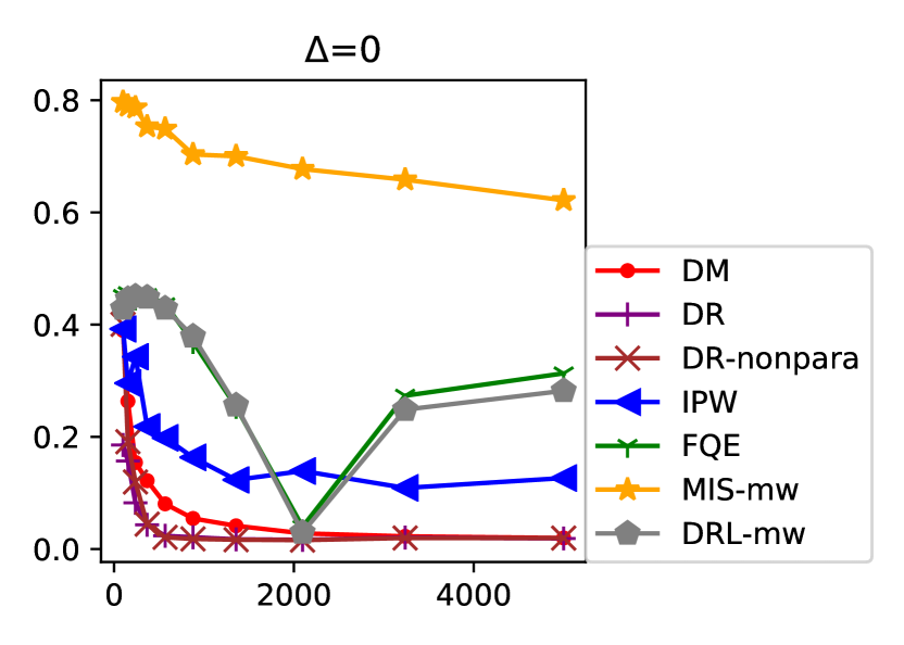
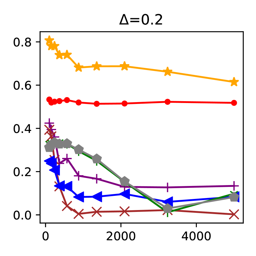
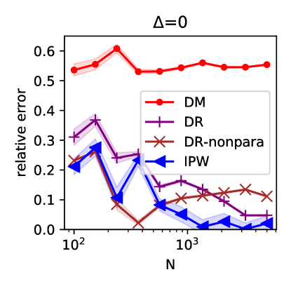
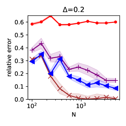
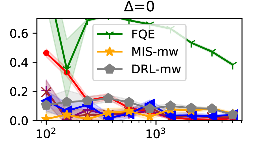
Policy evaluation and optimization. In Figureย 3 we generate different outcome models with increasing levels of misspecification $\Delta$, evaluate V0ฯ€eโ€‹(s0)superscriptsubscript๐‘‰0subscript๐œ‹๐‘’subscript๐‘ 0V_{0}^{\pi_{e}}(s_{0}) by Monte Carlo rollouts with $N=10000$ trajectories. We compare $\operatorname{DM}$ with logistic regression nuisance, $\operatorname{DR}$ doubly-robust with logistic regression, $\operatorname{DR-nonpara}$ with nonparametric nuisance, and $\operatorname{IPW}$, inverse propensity weighting. (See Sectionย D for further comparison including other baselines and policy optimization in the well-specified $\Delta=0$ case, where the variance drawbacks of $\operatorname{IPW}$ do worse than model-based approaches.) Figureย 2(a) considers off policy evaluation, with absolute relative error on the y-axis and trajectory size on the x-axis (log grid from $N=50,\dots 5000$). When $\Delta=0.2$ the logistic outcome model is misspecified, but orthogonality and the well-specified propensity score ensures estimates are asymptotically unbiased. Similar to other DR settings, although incorporating the outcome model reduces variance, incorporating a misspecified outcome model does worse than just using well-specified $\operatorname{IPW}$, but we see faster convergence from the flexible, nonparametric nuisance which outperforms well-specified $\operatorname{IPW}$. We also compared to nonparametric baselines FQE [35], and modified stateful versions of MIS [58] and DRL [30]. However, in this simple setting, the highly flexible nuisance estimators overfit and fail (incurring 40-50% absolute error). We discuss these baselines in greater detail in โ€œOPE comparisonโ€ in a more favorable data-generating process.

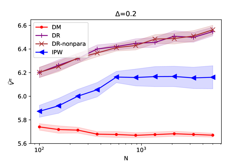
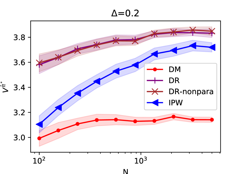
We then consider policy optimization in Figureย 2(b), with a rich policy class to avoid misspecification error issues. Motivated by eq.ย 8, observe that the optimal threshold policy on the true $\Delta\mu$ is an affine transform relative to a threshold on the estimated $\Delta\hat{\mu}$ (possibly misspecified, hence biased), with an $x$-conditional term for the conditional error. We approximate optimizing over policies $\mathbb{I}[\Delta\mu>\theta]$ by ranging over all thresholds on $\mathbb{I}[\Delta{\hat{\mu}}>\theta^{\prime}]$; this approximates the $x$-conditional error term of eq.ย 8 by a constant. This is similar to a contextual version of โ€œbid-priceโ€ policies [24]. We optimize over the class of threshold policies on $\Delta{\hat{\mu}}$ by enumerating thresholds and evaluating via the estimate from Propositionย 2, so the functional specification does depend on the (unadjusted) nuisance estimation. (Therefore the VC dimension of this depends on the VC dimension of the outcome nuisance). The $y$-axis depicts out of sample value (higher is better) averaged over 48 replications. Both $\operatorname{DR}$ and $\operatorname{IPW}$ (inverse propensity-weighted) estimates translate to improvements in optimized policy value. We see dramatic benefits of $\operatorname{DR}$ when $\Delta=0.2$. For small dataset sizes, $\operatorname{IPW}$ suffers from high variance as expected. Therefore, $\operatorname{DR}$ and its variance reduction estimates achieve sizeable improvements for small amounts of data. As the amount of data grows larger, the performance of $\operatorname{IPW}$ nears that of $\operatorname{DR}$ asymptotically. The DM plug-in approach remains biased and achieves worse performance, even asymptotically.

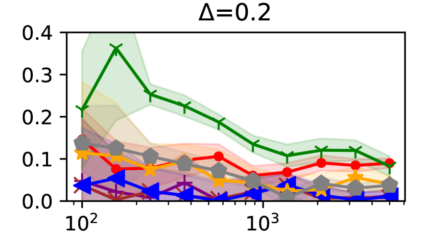
OPE comparison. We compare to state-of-the-art OPE: $\operatorname{FQE}$ of [35] which does not use the โ€œstatefulโ€ structure, and we also derive โ€œstrong baselinesโ€ that leverage some of the structure ($\operatorname{MIS-mw}$ [58], $\operatorname{DRL-mw}$ [31]). (We reiterate our core contribution is not in general off-policy evaluation but in deriving improvements for this specific structure). For example, observe that since $x$ is exogenously generated the finite-horizon state-action density ratio is independent of $x$. We endow $\operatorname{MIS-mw}$ and $\operatorname{DRL-mw}$ with this structural information (see appendix Sectionย D for details). As the general OPE literature prescribes, we use nonparametric nuisances, e.g. multi-layer perceptron with $\operatorname{scikit-learn}$ defaults for all nuisance predictors. We consider a more favorable DGP for OPE comparison in Figureย 2(c), using eq.ย 9 with $p=5$ and $\beta=[-0.53,-0.56,-0.10,0.40,0.74],\beta_{0}=-2.39$. $\operatorname{MIS-mw}$ does well overall, although empirically we find other DGPs where $\operatorname{MIS-mw}$ underperforms $\operatorname{FQE}$. In the misspecified setting, our doubly robust estimators outperform $\operatorname{MIS-mw}$. $\operatorname{FQE}$, which fits next time-step Qโ€‹(s,x,a),๐‘„๐‘ ๐‘ฅ๐‘ŽQ(s,x,a), appears to converge but much slower than our approaches. The gap between $\operatorname{FQE}$ and $\operatorname{DM}$ for the (slightly misspecified) case precisely illustrates the benefits of encoding problem structure in Equationย 1.

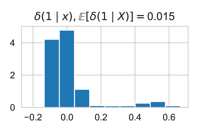
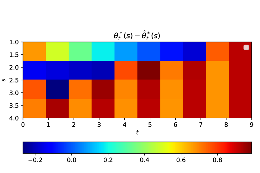
Assessing the structural conditions of Theoremย 3 in practice. In Figureย 3 we investigate assumptions made in Exampleย 4 (e.g. uniformity of error direction $\delta(1,x)$) that do not hold exactly. Figureย 2(d) plots $\delta$: although it is symmetrically distributed for most $x$, there is overall marginal error in the expected direction. In the empirical example we optimize over marginal thresholds and so we expect, marginalizing over x, the directional error condition is satisfied. In Figureย 2(e), we show a heatmap of ฮธtโˆ—โ€‹(s)โˆ’ฮธ^tโ€‹(s)superscriptsubscript๐œƒ๐‘ก๐‘ subscript^๐œƒ๐‘ก๐‘ \theta_{t}^{*}(s)-\hat{\theta}_{t}(s) over timesteps and state values. As the analysis suggests, for s>2๐‘ 2s>2 for most timesteps the error persists: red indicates regions where naive thresholds are in the same direction, relative to the optimal threshold, and hence the error persists rather than attenuates over time.

7 Conclusion

By studying the causal structure of practically relevant problems in operations, we developed specialized off policy evaluation and optimization which demonstrate the offline version of such problems is easier than a generic MDP. We show analytically that confounding matters, and verify our approach, reducing from $T+1$ nuisances to $2$ and estimating the expectation of a transition via the expectation over a population, achieves practical benefits. Future directions include function approximation in s๐‘ s and generalizing to other hierarchical structure.

References

  • Agrawal and Jia [2019] S.ย Agrawal and R.ย Jia. Learning in structured mdps with convex cost functions: Improved regret bounds for inventory management. In Proceedings of the 2019 ACM Conference on Economics and Computation, pages 743โ€“744, 2019.
  • Agrawal etย al. [2016] S.ย Agrawal, N.ย R. Devanur, and L.ย Li. An efficient algorithm for contextual bandits with knapsacks, and an extension to concave objectives. In Conference on Learning Theory, pages 4โ€“18, 2016.
  • Antos etย al. [2007] A.ย Antos, R.ย Munos, and C.ย Szepesvari. Fitted q-iteration in continuous action-space mdps. In Neural Information Processing Systems, 2007.
  • Badanidiyuru etย al. [2018] A.ย Badanidiyuru, R.ย Kleinberg, and A.ย Slivkins. Bandits with knapsacks. Journal of the ACM (JACM), 65(3):1โ€“55, 2018.
  • Ban and Keskin [2020] G.-Y. Ban and N.ย B. Keskin. Personalized dynamic pricing with machine learning: High dimensional features and heterogeneous elasticity. Forthcoming, Management Science, 2020.
  • Bertsekas and Tsitsiklis [1996] D.ย P. Bertsekas and J.ย N. Tsitsiklis. Neuro-dynamic programming. Athena Scientific, 1996.
  • Besbes and Zeevi [2012] O.ย Besbes and A.ย Zeevi. Blind network revenue management. Operations research, 60(6):1537โ€“1550, 2012.
  • Bibaut etย al. [2019] A.ย F. Bibaut, I.ย Malenica, N.ย Vlassis, and M.ย J. vanย der Laan. More efficient off-policy evaluation through regularized targeted learning. arXiv preprint arXiv:1912.06292, 2019.
  • Bimpikis etย al. [2019] K.ย Bimpikis, O.ย Candogan, and D.ย Saban. Spatial pricing in ride-sharing networks. Operations Research, 67(3):744โ€“769, 2019.
  • Bojun [2020] H.ย Bojun. Steady state analysis of episodic reinforcement learning. arXiv preprint arXiv:2011.06631, 2020.
  • Bray [2019] R.ย L. Bray. The multisecretary problem with continuous valuations. arXiv preprint arXiv:1912.08917, 2019.
  • Brockman etย al. [2016] G.ย Brockman, V.ย Cheung, L.ย Pettersson, J.ย Schneider, J.ย Schulman, J.ย Tang, and W.ย Zaremba. Openai gym. arXiv preprint arXiv:1606.01540, 2016.
  • Bumpensanti and Wang [2020] P.ย Bumpensanti and H.ย Wang. A re-solving heuristic with uniformly bounded loss for network revenue management. Management Science, 2020.
  • Chen and Jiang [2019] J.ย Chen and N.ย Jiang. Information-theoretic considerations in batch reinforcement learning. In International Conference on Machine Learning, pages 1042โ€“1051. PMLR, 2019.
  • Chen etย al. [2021] X.ย Chen, Z.ย Owen, C.ย Pixton, and D.ย Simchi-Levi. A statistical learning approach to personalization in revenue management. Management Science, 2021.
  • Chernozhukov etย al. [2018] V.ย Chernozhukov, D.ย Chetverikov, M.ย Demirer, E.ย Duflo, C.ย Hansen, W.ย Newey, and J.ย Robins. Double/debiased machine learning for treatment and structural parameters, 2018.
  • Cohen etย al. [2016] M.ย C. Cohen, I.ย Lobel, and R.ย P. Leme. Feature-based dynamic pricing. EC, 2016(10.1145):2940716โ€“2940728, 2016.
  • Duan etย al. [2020] Y.ย Duan, Z.ย Jia, and M.ย Wang. Minimax-optimal off-policy evaluation with linear function approximation. In International Conference on Machine Learning, pages 2701โ€“2709. PMLR, 2020.
  • Dudik etย al. [2014] M.ย Dudik, D.ย Erhan, J.ย Langford, and L.ย Li. Doubly robust policy evaluation and optimization. Statistical Science, 2014.
  • Elย Shar and Jiang [2020] I.ย Elย Shar and D.ย Jiang. Lookahead-bounded q-learning. In International Conference on Machine Learning, pages 8665โ€“8675. PMLR, 2020.
  • Emek etย al. [2020] Y.ย Emek, R.ย Lavi, R.ย Niazadeh, and Y.ย Shi. Stateful posted pricing with vanishing regret via dynamic deterministic markov decision processes. Advances in Neural Information Processing Systems, 33, 2020.
  • Farahmand and Szepesvรกri [2012] A.-m. Farahmand and C.ย Szepesvรกri. Regularized least-squares regression: Learning from a $\beta$-mixing sequence. Journal of Statistical Planning and Inference, 142(2):493โ€“505, 2012.
  • Gallego and Vanย Ryzin [1997] G.ย Gallego and G.ย Vanย Ryzin. A multiproduct dynamic pricing problem and its applications to network yield management. Operations research, 45(1):24โ€“41, 1997.
  • Gallego etย al. [2019] G.ย Gallego, H.ย Topaloglu, etย al. Revenue management and pricing analytics, volume 209. Springer, 2019.
  • Hu etย al. [2021] Y.ย Hu, N.ย Kallus, and M.ย Uehara. Fast rates for the regret of offline reinforcement learning. In Conference on Learning Theory, 2021.
  • Huh etย al. [2011] W.ย T. Huh, R.ย Levi, P.ย Rusmevichientong, and J.ย B. Orlin. Adaptive data-driven inventory control with censored demand based on kaplan-meier estimator. Operations Research, 59(4):929โ€“941, 2011.
  • Javanmard and Nazerzadeh [2016] A.ย Javanmard and H.ย Nazerzadeh. Dynamic pricing in high-dimensions. arXiv preprint arXiv:1609.07574, 2016.
  • Jiang and Li [2016] N.ย Jiang and L.ย Li. Doubly robust off-policy value evaluation for reinforcement learning. Proceedings of the 33rd International Conference on Machine Learning, 2016.
  • Jin etย al. [2018] C.ย Jin, Z.ย Allen-Zhu, S.ย Bubeck, and M.ย I. Jordan. Is q-learning provably efficient? arXiv preprint arXiv:1807.03765, 2018.
  • Kallus and Uehara [2019a] N.ย Kallus and M.ย Uehara. Double reinforcement learning for efficient off-policy evaluation in markov decision processes. arXiv preprint arXiv:1908.08526, 2019a.
  • Kallus and Uehara [2019b] N.ย Kallus and M.ย Uehara. Efficiently breaking the curse of horizon: Double reinforcement learning in infinite-horizon processes. arXiv preprint arXiv:1909.05850, 2019b.
  • Kallus and Zhou [2020] N.ย Kallus and A.ย Zhou. Minimax-optimal policy learning under unobserved confounding. Management Science, 2020.
  • Kennedy etย al. [2021] E.ย H. Kennedy, S.ย Balakrishnan, and L.ย Wasserman. Semiparametric counterfactual density estimation. arXiv preprint arXiv:2102.12034, 2021.
  • Kitagawa and Tetenov [2015] T.ย Kitagawa and A.ย Tetenov. Empirical welfare maximization. 2015.
  • Le etย al. [2019] H.ย Le, C.ย Voloshin, and Y.ย Yue. Batch policy learning under constraints. In International Conference on Machine Learning, pages 3703โ€“3712. PMLR, 2019.
  • Meyn and Meyn [2008] S.ย Meyn and S.ย P. Meyn. Control techniques for complex networks. Cambridge University Press, 2008.
  • Meyn and Tweedie [2012] S.ย P. Meyn and R.ย L. Tweedie. Markov chains and stochastic stability. Springer Science & Business Media, 2012.
  • Mohri etย al. [2018] M.ย Mohri, A.ย Rostamizadeh, and A.ย Talwalkar. Foundations of machine learning. MIT press, 2018.
  • Munos [2003] R.ย Munos. Error bounds for approximate policy iteration. In ICML, volumeย 3, pages 560โ€“567, 2003.
  • Munos [2007] R.ย Munos. Performance bounds in l_p-norm for approximate value iteration. SIAM journal on control and optimization, 46(2):541โ€“561, 2007.
  • Munos and Szepesvรกri [2008] R.ย Munos and C.ย Szepesvรกri. Finite-time bounds for fitted value iteration. Journal of Machine Learning Research, 9(5), 2008.
  • Nie etย al. [2020] X.ย Nie, E.ย Brunskill, and S.ย Wager. Learning when-to-treat policies. Journal of the American Statistical Association, pages 1โ€“18, 2020.
  • Pedregosa etย al. [2011] F.ย Pedregosa, G.ย Varoquaux, A.ย Gramfort, V.ย Michel, B.ย Thirion, O.ย Grisel, M.ย Blondel, P.ย Prettenhofer, R.ย Weiss, V.ย Dubourg, etย al. Scikit-learn: Machine learning in python. the Journal of machine Learning research, 12:2825โ€“2830, 2011.
  • Pollard [1990] D.ย Pollard. Empirical processes: theory and applications. NSF-CBMS regional conference series in probability and statistics, 1990.
  • Powell [2007] W.ย B. Powell. Approximate Dynamic Programming: Solving the curses of dimensionality, volume 703. John Wiley & Sons, 2007.
  • Qiang and Bayati [2016] S.ย Qiang and M.ย Bayati. Dynamic pricing with demand covariates. Available at SSRN 2765257, 2016.
  • Scherrer [2014] B.ย Scherrer. Approximate policy iteration schemes: a comparison. In International Conference on Machine Learning, pages 1314โ€“1322. PMLR, 2014.
  • Shah etย al. [2019] V.ย Shah, J.ย Blanchet, and R.ย Johari. Semi-parametric dynamic contextual pricing. arXiv preprint arXiv:1901.02045, 2019.
  • Swaminathan and Joachims [2015] A.ย Swaminathan and T.ย Joachims. The self-normalized estimator for counterfactual learning. Proceedings of NIPS, 2015.
  • Tang etย al. [2019] Z.ย Tang, Y.ย Feng, L.ย Li, D.ย Zhou, and Q.ย Liu. Doubly robust bias reduction in infinite horizon off-policy estimation. arXiv preprint arXiv:1910.07186, 2019.
  • Thomas and Brunskill [2016] P.ย Thomas and E.ย Brunskill. Data-efficient off-policy policy evaluation for reinforcement learning. In International Conference on Machine Learning, pages 2139โ€“2148, 2016.
  • Van Derย Vaart and Wellner [1996] A.ย W. Van Derย Vaart and J.ย A. Wellner. Weak convergence. In Weak convergence and empirical processes, pages 16โ€“28. Springer, 1996.
  • Vershynin [2018] R.ย Vershynin. High-dimensional probability: An introduction with applications in data science, volumeย 47. Cambridge University Press, 2018.
  • Wager and Athey [2017] S.ย Wager and S.ย Athey. Efficient policy learning. 2017.
  • Wainwright [2019] M.ย J. Wainwright. High-dimensional statistics: A non-asymptotic viewpoint, volumeย 48. Cambridge University Press, 2019.
  • Xie etย al. [2019] T.ย Xie, Y.ย Ma, and Y.-X. Wang. Towards optimal off-policy evaluation for reinforcement learning with marginalized importance sampling. arXiv preprint arXiv:1906.03393, 2019.
  • Yang and Barron [1999] Y.ย Yang and A.ย Barron. Information-theoretic determination of minimax rates of convergence. Annals of Statistics, pages 1564โ€“1599, 1999.
  • Yin etย al. [2021] M.ย Yin, Y.ย Bai, and Y.-X. Wang. Near-optimal provable uniform convergence in offline policy evaluation for reinforcement learning. In International Conference on Artificial Intelligence and Statistics, pages 1567โ€“1575. PMLR, 2021.
  • Zhang etย al. [2013] B.ย Zhang, A.ย A. Tsiatis, E.ย B. Laber, and M.ย Davidian. Robust estimation of optimal dynamic treatment regimes for sequential treatment decisions. Biometrika, 100(3):681โ€“694, 2013.
  • Zhao etย al. [2015] Y.-Q. Zhao, D.ย Zeng, E.ย B. Laber, and M.ย R. Kosorok. New statistical learning methods for estimating optimal dynamic treatment regimes. Journal of the American Statistical Association, 110(510):583โ€“598, 2015.
  • Zhou etย al. [2018] Z.ย Zhou, S.ย Athey, and S.ย Wager. Offline multi-action policy learning: Generalization and optimization. arXiv preprint arXiv:1810.04778, 2018.
Outline of appendix

Sectionย A analyzes the marginal MDP construction of Sectionย 4.

Sectionย B provides analysis of the main estimation strategy and policy learning sample complexity analysis, e.g. proofs of Sectionย 5.

Sectionย C provides additional discussion.

Sectionย D includes additional empirics and discussion of computational details.

A Proofs for Sectionย 4

Proof of Propositionย 1.

We argue via backwards induction, though the proof follows largely from construction of the marginal MDP. Consider the last timestep, $t=T$: equivalence follows by construction. Next consider the inductive step. The inductive hypothesis posits equivalence of policy values Vt+1โ€‹(s)subscript๐‘‰๐‘ก1๐‘ V_{t+1}(s) in the marginal MDP and V~t+1โ€‹(s)subscript~๐‘‰๐‘ก1๐‘ \tilde{V}_{t+1}(s), the marginalized policy value in the full-information MDP, as well as equivalence of optimal policies so that Vt+1โ€‹(s)=V~t+1โ€‹(s)subscript๐‘‰๐‘ก1๐‘ subscript~๐‘‰๐‘ก1๐‘ V_{t+1}(s)=\tilde{V}_{t+1}(s).

Recall that each policy ฯ€โˆˆฮ ๐œ‹ฮ \pi\in\Pi in $\mathcal{M}$ corresponds to an action ฯ€โˆˆฮ ๐œ‹ฮ \pi\in\Pi of $\widetilde{\mathcal{M}}$ with transition probability:

$$\tilde{P}(s^{\prime}\mid s,\pi)=P(Y=y\mid\pi)\mathrel{\hbox to0.0pt{\raisebox{1.29167pt}{$\cdot$}\hss}\raisebox{-1.29167pt}{$\cdot$}}=\int\int P(s^{\prime}\mid s,a,x)\pi(a\mid x)f(x)dx$$ (10)

Equivalence of the policy values follows from backwards induction of expected rewards and definition of the marginal MDPs. Equivalence of optimal policies follows from equivalence of first moments and equivalence of the policy classes. Equivalence of the inductive step follows from equivalence of policy classes, identically distributed arrivals $X_{i}$ within a timestep . โˆŽ

Proof of Propositionย 2.

Double robustness is standard and follows standard arguments in the single time-step policy learning literature [19, 54]. The claim follows by observing that by the restricted causal structure Assumptionย 2, $Y(a)\mathchoice{\mathrel{\hbox to0.0pt{$\displaystyle\perp$\hss}\mkern 2.0mu{\displaystyle\perp}}}{\mathrel{\hbox to0.0pt{$\textstyle\perp$\hss}\mkern 2.0mu{\textstyle\perp}}}{\mathrel{\hbox to0.0pt{$\scriptstyle\perp$\hss}\mkern 2.0mu{\scriptstyle\perp}}}{\mathrel{\hbox to0.0pt{$\scriptscriptstyle\perp$\hss}\mkern 2.0mu{\scriptscriptstyle\perp}}}S\mid X$, so it is sufficient to adjust for IPW weights ${P(A=a\mid X=x)}$.

For completeness, we verify double-robust unbiasedness properties of V^tโ€‹(s)subscript^๐‘‰๐‘ก๐‘ \hat{V}_{t}(s). The proof follows by backward induction. The fact that VT+1โ€‹(s)=0subscript๐‘‰๐‘‡1๐‘ 0V_{T+1}(s)=0 and estimation is unbiased follows from double-robustness in the single-timestep setting for V^Tโ€‹(s)subscript^๐‘‰๐‘‡๐‘ \hat{V}_{T}(s) for all sโˆˆ๐’ฎ๐‘ ๐’ฎs\in\mathcal{S}.

Next we show the inductive step. Suppose V^t+1โ€‹(s)subscript^๐‘‰๐‘ก1๐‘ \hat{V}_{t+1}(s) is unbiased, for all sโˆˆ๐’ฎ๐‘ ๐’ฎs\in\mathcal{S}. We require that the evaluation error is independent (V^t+1tDRโ€‹(sโ€ฒ)โˆ’Vt+1โ€‹(sโ€ฒ))superscriptsubscript^๐‘‰๐‘ก1tDRsuperscript๐‘ โ€ฒsubscript๐‘‰๐‘ก1superscript๐‘ โ€ฒ(\hat{V}_{t+1}^{\text{tDR}}(s^{\prime})-V_{t+1}(s^{\prime})) from the nuisance evaluation error, which can be easily satisfied by appropriate sample splitting.

If $\mu$ is unbiased:

๐”ผโ€‹[V^tโ€‹(s)]๐”ผdelimited-[]subscript^๐‘‰๐‘ก๐‘ \displaystyle\mathbb{E}[\widehat{V}_{t}(s)] =๐”ผโ€‹[โˆ‘sโ€ฒ,yโˆฃsโˆ‘aฯ€eโ€‹(aโˆฃx)โ€‹ฮผtโ€‹(yโˆฃa,x)โ€‹(Rโ€‹(y)+V^t+1tDRโ€‹(sโ€ฒ))]absent๐”ผdelimited-[]subscriptsuperscript๐‘ โ€ฒconditional๐‘ฆ๐‘ subscript๐‘Žsubscript๐œ‹๐‘’conditional๐‘Ž๐‘ฅsubscript๐œ‡๐‘กconditional๐‘ฆ๐‘Ž๐‘ฅ๐‘…๐‘ฆsuperscriptsubscript^๐‘‰๐‘ก1tDRsuperscript๐‘ โ€ฒ\displaystyle=\mathbb{E}\left[\sum_{s^{\prime},y\mid s}\sum_{a}\pi_{e}(a\mid x)\mu_{t}(y\mid a,x)(R(y)+\hat{V}_{t+1}^{\text{tDR}}(s^{\prime}))\right] (11)
+๐”ผโ€‹[โˆ‘sโ€ฒ,yโˆฃsโˆ‘aฯ€eโ€‹(aโˆฃx)โ€‹(๐•€โ€‹[At=a]ฯ€bโ€‹(aโˆฃx)โ€‹(๐•€โ€‹[Y=y]โˆ’ฮผtโ€‹(yโˆฃa,x)))โ€‹(Rโ€‹(y)+Vt+1โ€‹(sโ€ฒ))]๐”ผdelimited-[]subscriptsuperscript๐‘ โ€ฒconditional๐‘ฆ๐‘ subscript๐‘Žsubscript๐œ‹๐‘’conditional๐‘Ž๐‘ฅ๐•€delimited-[]subscript๐ด๐‘ก๐‘Žsubscript๐œ‹๐‘conditional๐‘Ž๐‘ฅ๐•€delimited-[]๐‘Œ๐‘ฆsubscript๐œ‡๐‘กconditional๐‘ฆ๐‘Ž๐‘ฅ๐‘…๐‘ฆsubscript๐‘‰๐‘ก1superscript๐‘ โ€ฒ\displaystyle\qquad+\mathbb{E}\left[\sum_{s^{\prime},y\mid s}\sum_{a}\pi_{e}(a\mid x)\left(\frac{\mathbb{I}\left[A_{t}=a\right]}{\pi_{b}(a\mid x)}\left(\mathbb{I}\left[Y=y\right]-\mu_{t}(y\mid a,x)\right)\right)(R(y)+V_{t+1}(s^{\prime}))\right] (12)
+๐”ผโ€‹[โˆ‘sโ€ฒ,yโˆฃsโˆ‘aฯ€eโ€‹(aโˆฃx)โ€‹(๐•€โ€‹[At=a]ฯ€bโ€‹(aโˆฃx)โ€‹(๐•€โ€‹[Y=y]โˆ’ฮผtโ€‹(yโˆฃa,x)))โ€‹(V^t+1tDRโ€‹(sโ€ฒ)โˆ’Vt+1โ€‹(sโ€ฒ))]๐”ผdelimited-[]subscriptsuperscript๐‘ โ€ฒconditional๐‘ฆ๐‘ subscript๐‘Žsubscript๐œ‹๐‘’conditional๐‘Ž๐‘ฅ๐•€delimited-[]subscript๐ด๐‘ก๐‘Žsubscript๐œ‹๐‘conditional๐‘Ž๐‘ฅ๐•€delimited-[]๐‘Œ๐‘ฆsubscript๐œ‡๐‘กconditional๐‘ฆ๐‘Ž๐‘ฅsuperscriptsubscript^๐‘‰๐‘ก1tDRsuperscript๐‘ โ€ฒsubscript๐‘‰๐‘ก1superscript๐‘ โ€ฒ\displaystyle\qquad+\mathbb{E}\left[\sum_{s^{\prime},y\mid s}\sum_{a}\pi_{e}(a\mid x)\left(\frac{\mathbb{I}\left[A_{t}=a\right]}{\pi_{b}(a\mid x)}\left(\mathbb{I}\left[Y=y\right]-\mu_{t}(y\mid a,x)\right)\right)(\hat{V}_{t+1}^{\text{tDR}}(s^{\prime})-V_{t+1}(s^{\prime}))\right] (13)

Note eq.ย 11 =Vtโ€‹(s)absentsubscript๐‘‰๐‘ก๐‘ =V_{t}(s) by well-specification, eq.ย 12 $=0$ by unbiasedness of $\mu_{t}$ and cross-fitting so the estimation errors are independent, and the first term of eq.ย 13 is expectation-0 by the previous argument and ๐”ผโ€‹[(V^t+1tDRโ€‹(sโ€ฒ)โˆ’Vt+1โ€‹(sโ€ฒ))]=0๐”ผdelimited-[]superscriptsubscript^๐‘‰๐‘ก1tDRsuperscript๐‘ โ€ฒsubscript๐‘‰๐‘ก1superscript๐‘ โ€ฒ0\mathbb{E}[(\hat{V}_{t+1}^{\text{tDR}}(s^{\prime})-V_{t+1}(s^{\prime}))]=0 by the induction hypothesis and cross-fitting.

If $e$ is unbiased:

๐”ผโ€‹[V^tโ€‹(s)]๐”ผdelimited-[]subscript^๐‘‰๐‘ก๐‘ \displaystyle\mathbb{E}[\widehat{V}_{t}(s)]
=๐”ผโ€‹[โˆ‘sโ€ฒ,yโˆฃsโˆ‘aฯ€eโ€‹(aโˆฃx)โ€‹(๐•€โ€‹[At=a]ฯ€bโ€‹(aโˆฃx)โ€‹๐•€โ€‹[Y=y]โŸunbiased IPW estimator+ฮผtโ€‹(yโˆฃa,x)โ€‹(1โˆ’๐•€โ€‹[At=a]ฯ€bโ€‹(aโˆฃx))โŸ=0โ€‹ย by unbiasedness ofย โ€‹e)โ€‹(Rโ€‹(y)+Vt+1โ€‹(sโ€ฒ))]absent๐”ผdelimited-[]subscriptsuperscript๐‘ โ€ฒconditional๐‘ฆ๐‘ subscript๐‘Žsubscript๐œ‹๐‘’conditional๐‘Ž๐‘ฅsubscriptโŸ๐•€delimited-[]subscript๐ด๐‘ก๐‘Žsubscript๐œ‹๐‘conditional๐‘Ž๐‘ฅ๐•€delimited-[]๐‘Œ๐‘ฆunbiased IPW estimatorsubscript๐œ‡๐‘กconditional๐‘ฆ๐‘Ž๐‘ฅsubscriptโŸ1๐•€delimited-[]subscript๐ด๐‘ก๐‘Žsubscript๐œ‹๐‘conditional๐‘Ž๐‘ฅabsent0ย by unbiasedness ofย ๐‘’๐‘…๐‘ฆsubscript๐‘‰๐‘ก1superscript๐‘ โ€ฒ\displaystyle=\mathbb{E}\left[\sum_{s^{\prime},y\mid s}\sum_{a}\pi_{e}(a\mid x)\left(\underbrace{\frac{\mathbb{I}\left[A_{t}=a\right]}{\pi_{b}(a\mid x)}\mathbb{I}\left[Y=y\right]}_{\text{unbiased IPW estimator}}+\mu_{t}(y\mid a,x)\underbrace{\left(1-\frac{\mathbb{I}\left[A_{t}=a\right]}{\pi_{b}(a\mid x)}\right)}_{=0\text{ by unbiasedness of }e}\right)(R(y)+V_{t+1}(s^{\prime}))\right]
+๐”ผโ€‹[โˆ‘sโ€ฒ,yโˆฃsโˆ‘aฯ€eโ€‹(aโˆฃx)โ€‹(ฮผtโ€‹(yโˆฃa,x)โ€‹(1โˆ’๐•€โ€‹[At=a]ฯ€bโ€‹(aโˆฃx))โŸ=0โ€‹ย by unbiasedness ofย โ€‹e)โ€‹(V^t+1tDRโ€‹(sโ€ฒ)โˆ’Vt+1โ€‹(sโ€ฒ))โŸ=0โ€‹ย by inductive hypothesisย ]๐”ผdelimited-[]subscriptsuperscript๐‘ โ€ฒconditional๐‘ฆ๐‘ subscript๐‘Žsubscript๐œ‹๐‘’conditional๐‘Ž๐‘ฅsubscript๐œ‡๐‘กconditional๐‘ฆ๐‘Ž๐‘ฅsubscriptโŸ1๐•€delimited-[]subscript๐ด๐‘ก๐‘Žsubscript๐œ‹๐‘conditional๐‘Ž๐‘ฅabsent0ย by unbiasedness ofย ๐‘’subscriptโŸsuperscriptsubscript^๐‘‰๐‘ก1tDRsuperscript๐‘ โ€ฒsubscript๐‘‰๐‘ก1superscript๐‘ โ€ฒabsent0ย by inductive hypothesisย \displaystyle+\mathbb{E}\left[\sum_{s^{\prime},y\mid s}\sum_{a}\pi_{e}(a\mid x)\left(\mu_{t}(y\mid a,x)\underbrace{\left(1-\frac{\mathbb{I}\left[A_{t}=a\right]}{\pi_{b}(a\mid x)}\right)}_{=0\text{ by unbiasedness of }e}\right)\underbrace{(\hat{V}_{t+1}^{\text{tDR}}(s^{\prime})-V_{t+1}(s^{\prime}))}_{=0\text{ by inductive hypothesis }}\right]

โˆŽ

B Proofs for Sectionย 5

B.1 Sample complexity proofs

B.1.1 Concentration preliminaries

We introduce the uniform convergence setup we use to provide tail inequalities. We will apply a standard chaining argument with Orlicz norms and introduce some notations from standard references, e.g. [53, 44, 55]. A function $\phi:[0,\infty)\to[0,\infty)$ is an Orlicz function if $\phi$ is convex, increasing, and satisfies $\phi(0)=0,\phi(x)\to\infty$ as $x\to\infty$. For a given Orlicz function $\phi$, the Orlicz norm of a random variable $X$ is defined as $\left\lVert X\right\rVert_{\phi}=\inf\{t>0\colon\mathbb{E}[\Phi(\left\lVert X\right\rVert\mid t)]\leq 1\}$. The Orlicz norm $\left\lVert Z\right\rVert_{\Phi}$ of random variable $Z$ is defined by $\left\lVert Z\right\rVert_{\Phi}=\inf\{C>0\colon\mathbb{E}[\Phi(Z/C)]\leq 1\}.$ A constant bound on $\left\lVert Z\right\rVert_{\Phi}$ constrains the rate of decrease for the tail probabilities by the inequality $\mathbb{P}(|Z|\geq t)\leq 1/\Phi(t/C)$ if $C=\left\lVert Z\right\rVert_{\Phi}$. For example, choosing the Orlicz function $\Phi(t)=\frac{1}{5}\exp(t^{2})$ results in bounds by subgaussian tails decreasing like $\exp(-Ct^{2})$, for some constant $C$.

We next introduce the tail inequalities that use a standard chaining argument to control uniform convergence over ฯ€โˆˆฮ ๐œ‹ฮ \pi\in\Pi. Let $n$ denote a generic dataset size (we will later on apply the results with $n=NT$.) The data are $(X_{1:n},A_{1:n},Y_{1:n})$ and $f_{i}(\pi)$ is a function of $(X_{i},A_{i},Y_{i})$. Define the function class โ„ฑโ€‹(X1:n,A1:n,Y1:n)={(fiโ€‹(ฯ€),โ€ฆ,fnโ€‹(ฯ€)):ฯ€โˆˆฮ }.โ„ฑsubscript๐‘‹:1๐‘›subscript๐ด:1๐‘›subscript๐‘Œ:1๐‘›conditional-setsubscript๐‘“๐‘–๐œ‹โ€ฆsubscript๐‘“๐‘›๐œ‹๐œ‹ฮ \mathcal{F}(X_{1:n},A_{1:n},Y_{1:n})=\{(f_{i}(\pi),\dots,f_{n}(\pi))\colon\pi\in\Pi\}.

For this section, we consider maximal inequalities for the function classes for the enveloped policy class $\mathcal{F}$. Let $\epsilon_{i}\in\{-1,+1\}$, be iid Rademacher variables (symmetric Bernoulli random variables with value $-1,+1$ with probability $\frac{1}{2}$), distributed independently of all else. We use the following application of chaining with a bounded envelope function, due to [44, Eqn. 7.3]. (Using different measures of functional complexity for multi-class predictors, such as Natarajan dimension, simply changes the constants in the final bound.)

Theorem A (Uniform convergence of policy function $\pi$ over envelope class $\mathcal{F}$. ).

Let $f(\pi)\leq\left\lVert F\right\rVert_{2}\leq C$ be a bound on the envelope function for $f\in\mathcal{F}$. Then for $n$ large enough, where $d_{\operatorname{vc}}$ is the VC-dimension,

$$\sup_{f\in\mathcal{F}}\left|\frac{1}{n}\sum_{i=1}^{n}(f_{i}(\pi)-\mathbb{E}[f(\pi)])\right|\leq\nicefrac{{9}}{{2}}C\sqrt{\frac{d_{\operatorname{vc}}\log(\nicefrac{{5}}{{\delta}})}{{n}}}$$ (14)

The next variant is a modification of Thm. A which only uses only moment bounds for the envelope function at the expense of weaker controls of the tails of the supremum process.

Theorem B (Uniform convergence with $L_{p}$ norm of envelope function.).

For an absolute constant $C_{d_{\operatorname{vc}}}$ which depends only on $d_{\operatorname{vc}}$, where $F_{n}$ is the envelope for $f\in\mathcal{F}$ and $d_{\operatorname{vc}}$ is the VC dimension, $\textstyle\mathbb{E}[\sup_{f\in\mathcal{F}}\left|\frac{1}{n}\sum_{i=1}^{n}(f_{i}(\pi)-\mathbb{E}[f(\pi)])\right|]\leq C_{d_{\operatorname{vc}}}^{\prime}\sqrt{d_{\operatorname{vc}}-1}\mathbb{E}[\left|F_{n}\right|]$.

We also state a standard lemma used for sample splitting, as appears in [16], without proof.

Lemma 1 (Conditional convergence implies unconditional).

Let $\{X_{m}\}$ and $\{Y_{m}\}$ be sequences of random vectors.

  • โ€ข

    If for $\epsilon_{m}\to 0$, $\mathbb{P}(\left\lVert X_{m}\right\rVert>\epsilon_{m}\mid Y_{m})\to_{p}0,$ then $\mathbb{P}(\left\lVert X_{m}\right\rVert>\epsilon_{m})\to 0.$ This occurs if $\mathbb{E}[\left\lVert X_{m}\right\rVert^{q}/\epsilon_{m}^{q}\mid Y_{m}]\to_{p}0$ for some $q\geq 1$ by Markovโ€™s inequality.

  • โ€ข

    Let $\{A_{m}\}$ be a sequence of positive constants. If $\left\lVert X_{m}\right\rVert=O_{p}(A_{m})$ conditional on $Y_{m}$, that for any $\ell_{m}\to\infty$, $\mathbb{P}(\left\lVert X_{m}\right\rVert>\ell_{m}A_{m}\mid Y_{m})\to_{p}0,$ then $\left\lVert X_{m}\right\rVert=O_{p}(A_{m})$ unconditionally, namely, that for any $\ell_{m}\to\infty$, then $\mathbb{P}(\left\lVert X_{m}\right\rVert>\ell_{m}A_{m})\to 0$.

Proof of Thm.ย A.

We first bound the deviations uniformly over the policy class and introduce the following empirical processes,

$$M=\sup_{f\in\mathcal{F}}\left|\sum_{i=1}^{n}(f_{i}(\pi)-\mathbb{E}[f(\pi)])\right|,\quad L=\sup_{f\in\mathcal{F}}\left|\sum_{i=1}^{n}\epsilon_{i}f_{i}(\pi)\right|.$$

By a standard symmetrization argument, applying Jensenโ€™s inequality for the convex function $\Phi$ of the symmetrized process (e.g. Theorem 2.2 of [44]), we may bound the Orlicz norm of the maxima of the empirical process by the symmetrized process, conditional on the observed data: $\mathbb{E}[\Phi(M)]\leq\mathbb{E}[\Phi(2L)].$ Taking Orlicz norms with $\Phi(t)=\frac{1}{5}\exp(t^{2})$, we apply a tail inequality on the Orlicz norm of the symmetrized process $\Phi\left(2L\right)$, under the assumption of bounded outcomes. Applying Dudleyโ€™s inequality to the symmetrized empirical process $L$, (e.g. Theorem 3.5 of [44]), we have that

$$\mathbb{E}_{\epsilon}\left[\exp(L^{2}/J^{2})\mid\mathcal{D}\right]\leq 5~{}~{}\text{for}~{}~{}J=9\left\|F\right\|_{2}\int_{0}^{1}\sqrt{\log(D(\left\|F\right\|_{2}\zeta,\mathcal{F}(X_{1:n})))}d\zeta.$$ (15)

By Markovโ€™s inequality, we have that $\mathbb{P}\left(\frac{1}{n}L>t\right)\leq 5\exp(-t^{2}n^{2}/\left\lVert L\right\rVert^{2}_{2})=5\exp(-t^{2}n/J^{2}C^{2}),$ so that therefore, bounding the Dudley entropy integral by the VC dimension via [44, eqn. 7.8],

$$\frac{1}{n}M\leq\frac{\nicefrac{{9}}{{2}}C\sqrt{d_{\operatorname{vc}}\log(\nicefrac{{5}}{{\delta}})}}{\sqrt{n}}.$$

โˆŽ

Proof of Thm.ย B.

By standard results on covering numbers and VC dimension, e.g. [52, 55], for a VC-class of functions with measurable envelope function $F$ and $p\geq 1$, for any probability measure $Q$ with $\left\lVert F\right\rVert_{Q,p}>0$, $N(\epsilon\left\lVert F\right\rVert_{Q,p},\mathcal{F},L_{p}(Q))\leq A(d_{\operatorname{vc}})(\frac{1}{\epsilon})^{p(d_{\operatorname{vc}}-1)}$, where $C_{d_{\operatorname{vc}}})$ is an absolute constant that depends only on the vc-dimension. By [44, eqn. 7.8],

$\displaystyle\textstyle\mathbb{E}[\sup_{\pi}\left|\frac{1}{n}\sum_{i=1}^{n}(f_{i}(\pi)-\mathbb{E}[f(\pi)])\right|^{p}]$ $\displaystyle\leq\left(18C_{p}\int_{0}^{1}\sqrt{\log\left(C_{d_{\operatorname{vc}}}\left(\nicefrac{{1}}{{\epsilon}}\right)^{p(d_{\operatorname{vc}}-1)}\right)}dx\right)\mathbb{E}[\left|F_{n}\right|^{p}]$
$\displaystyle\leq C_{d_{\operatorname{vc}}}^{\prime}\sqrt{d_{\operatorname{vc}}-1}\mathbb{E}[\left|F_{n}\right|^{p}]$

The claim follows by taking $p=2$. โˆŽ

Preliminaries

A key step of the analysis is leveraging an additive decomposition of the regret for finite horizons. For example, this appears in [29]; we simply include the full statement for completeness and verify for our setting. Recall that we denote $\tilde{P}$ as the transition matrices and estimated transition matrices corresponding to the marginal MDP (e.g. transitions between system states). In this section, for brevity we let $\widehat{{P}}$ denote the empirical counterpart of $\tilde{P}$, e.g. estimating eq.ย 2 via some estimation strategy (IPW weighting, doubly robust, or plug-in estimation; typically we focus on the doubly-robust estimator). Similarly, $\widehat{M}$ denotes the empirical MDP model with $\widehat{{P}}$. We introduce notation for indexing into entries after evaluating the transition operator,

$$(\tilde{P}V)(s,\pi)=\mathbb{E}_{s^{\prime}\sim\tilde{P}(\cdot\mid s,\pi)}V(s^{\prime})=\mathbb{E}[\tilde{R}(s,\pi)]+\sum_{(s^{\prime},y)\mid s}P(Y=y\mid\pi)(V(s^{\prime}))$$

We also introduce notation for indexing the difference between applying the true transition operator and the empirical estimate thereof, for any generic $|\mathcal{S}|$-vector v and policy $\pi$:

((P~โˆ’P^)โ€‹v)โ€‹(s,ฯ€)=โˆ‘(sโ€ฒ,y)โˆฃs(Pโ€‹(Y=yโˆฃฯ€)โˆ’P^โ€‹(Y=yโˆฃฯ€))โ€‹vโ€‹(sโ€ฒ).~๐‘ƒ^๐‘ƒ๐‘ฃ๐‘ ๐œ‹subscriptconditionalsuperscript๐‘ โ€ฒ๐‘ฆ๐‘ ๐‘ƒ๐‘Œconditional๐‘ฆ๐œ‹^๐‘ƒ๐‘Œconditional๐‘ฆ๐œ‹๐‘ฃsuperscript๐‘ โ€ฒ((\tilde{P}-\widehat{{P}})v)(s,\pi)=\sum_{(s^{\prime},y)\mid s}\left(P(Y=y\mid\pi)-\hat{P}(Y=y\mid\pi)\right)v(s^{\prime}).
Lemma 2 (Additive decomposition of finite-horizon value iteration).

For any policies $\tilde{\pi},\pi$ and any (s,tโ€ฒ)โˆˆ๐’ฎร—[T]๐‘ superscript๐‘กโ€ฒ๐’ฎdelimited-[]๐‘‡(s,t^{\prime})\in\mathcal{S}\times[T],

V~tโ€ฒฯ€~โ€‹(s)โˆ’V^tโ€ฒฯ€โ€‹(s)superscriptsubscript~๐‘‰superscript๐‘กโ€ฒ~๐œ‹๐‘ subscriptsuperscript^๐‘‰๐œ‹superscript๐‘กโ€ฒ๐‘ \displaystyle\tilde{V}_{t^{\prime}}^{\tilde{\pi}}(s)-\widehat{{V}}^{\pi}_{t^{\prime}}(s)
=๐”ผM^,ฯ€~โ€‹[โˆ‘t=tโ€ฒT๐”ผโ€‹[R~โ€‹(s,ฯ€t)]โˆ’๐”ผ^โ€‹[R~โ€‹(s,ฯ€t)]+โˆ‘(sโ€ฒ,y)โˆฃs(Pโ€‹(Y=yโˆฃฯ€t)โˆ’โ„™^โ€‹(Y=yโˆฃฯ€t))โ€‹V~t+1ฯ€โ€‹(sโ€ฒ)โˆฃst=s]absentsubscript๐”ผ^๐‘€~๐œ‹delimited-[]superscriptsubscript๐‘กsuperscript๐‘กโ€ฒ๐‘‡๐”ผdelimited-[]~๐‘…๐‘ subscript๐œ‹๐‘ก^๐”ผdelimited-[]~๐‘…๐‘ subscript๐œ‹๐‘กconditionalsubscriptconditionalsuperscript๐‘ โ€ฒ๐‘ฆ๐‘ ๐‘ƒ๐‘Œconditional๐‘ฆsubscript๐œ‹๐‘ก^โ„™๐‘Œconditional๐‘ฆsubscript๐œ‹๐‘กsuperscriptsubscript~๐‘‰๐‘ก1๐œ‹superscript๐‘ โ€ฒsubscript๐‘ ๐‘ก๐‘ \displaystyle=\mathbb{E}_{\hat{M},\tilde{\pi}}\left[\sum\nolimits_{t=t^{\prime}}^{T}\mathbb{E}[\tilde{R}(s,\pi_{t})]-\hat{\mathbb{E}}[\tilde{R}(s,\pi_{t})]+\sum\nolimits_{(s^{\prime},y)\mid s}\left(P(Y=y\mid\pi_{t})-\hat{\mathbb{P}}(Y=y\mid\pi_{t})\right)\tilde{V}_{t+1}^{\pi}(s^{\prime})\mid s_{t}=s\right]

B.2 Sample complexity analysis

We first provide a generalization bound in an oracle nuisance case where we use the true conditional expectations $\mu,e$ rather than estimated counterparts $\hat{\mu},\hat{e}$.

$\displaystyle\Gamma_{t}^{i,*}(y\mid a)$ $\displaystyle\mathrel{\hbox to0.0pt{\raisebox{1.29167pt}{$\cdot$}\hss}\raisebox{-1.29167pt}{$\cdot$}}=\frac{\mathbb{I}[Y_{t}^{i}=y]-{\mu}(y\mid A_{t}^{i},X_{t}^{i})}{{e}\left(A_{t}^{i}\mid X_{t}^{i}\right)}\mathbb{I}[A_{t}^{i}=a]+{{\mu}}(y\mid a,X_{t}^{i})$ (16)
$\displaystyle\hat{P}(Y=y\mid\pi)$ $\displaystyle\textstyle\mathrel{\hbox to0.0pt{\raisebox{1.29167pt}{$\cdot$}\hss}\raisebox{-1.29167pt}{$\cdot$}}=\frac{1}{NT}\sum_{t=1}^{T}\sum_{i=1}^{N}\sum_{a\in\mathcal{A}}\pi(a\mid X_{t}^{i})\hat{\Gamma}_{t}^{i,*}(y\mid a)$
Theorem 4 (Sample complexity and rate double-robustness for oracle estimator ).

Suppose ${e(a\mid x)\leq\nu^{-1}}$ uniformly over $a,x$ (overlap).

Then w.p. $\geq 1-\delta$, for $\tilde{V}^{\hat{\pi}^{*}}_{0}$ optimized via Algorithmย 1 with oracle nuisance estimator eq.ย 16,

$$\tilde{V}^{\pi^{*}}_{0}-\tilde{V}^{\hat{\pi}^{*}_{\operatorname{oracle}}}_{0}\leq\frac{\nu d_{\operatorname{vc}}R^{\max}(T+\nicefrac{{1}}{{2}}T^{2})\nicefrac{{9}}{{2}}\sqrt{\log(\nicefrac{{5T|\mathcal{Y}|}}{{\delta}})}}{\sqrt{NT}}$$
Proof of Theoremย 4.

In the analysis, we leverage single-timestep uniform convergence arguments. By Assumptionย 1, $X$ is drawn exogenously/independently of all else, so the $X$ data is iid. We model the dataset as drawn from multiple behavior policies, so that at timestep $t$, Sโˆผฯtฯ€bโ€‹(S),Xโˆผft,Aโˆผฯ€bโ€‹(s,x)formulae-sequencesimilar-to๐‘†superscriptsubscript๐œŒ๐‘กsubscript๐œ‹๐‘๐‘†formulae-sequencesimilar-to๐‘‹subscript๐‘“๐‘กsimilar-to๐ดsubscript๐œ‹๐‘๐‘ ๐‘ฅS\sim\rho_{t}^{\pi_{b}}(S),X\sim f_{t},A\sim\pi_{b}(s,x), and $Y\mid A,X$ is drawn from the contextual response model. Therefore the data tuples $(S_{i,t},X_{i,t},A_{i,t},Y_{i,t})$ are viewed as independent draws from this process. Since $Y\mid A,X\mathchoice{\mathrel{\hbox to0.0pt{$\displaystyle\perp$\hss}\mkern 2.0mu{\displaystyle\perp}}}{\mathrel{\hbox to0.0pt{$\textstyle\perp$\hss}\mkern 2.0mu{\textstyle\perp}}}{\mathrel{\hbox to0.0pt{$\scriptstyle\perp$\hss}\mkern 2.0mu{\scriptstyle\perp}}}{\mathrel{\hbox to0.0pt{$\scriptscriptstyle\perp$\hss}\mkern 2.0mu{\scriptscriptstyle\perp}}}S_{t}$ and therefore we only need to control for $X_{t}$ such that $e(X_{t})$ is not a function of $S$, the functions we use in our estimator, defined with respect only to the $(X_{i,t},A_{i,t},Y_{i,t})$ data, admit analysis via iid/single-stage empirical process techniques.

We define the following function classes conditional on all the data, $(X_{1:NT},A_{1:NT},Y_{1:NT})$. For $\pi$, we consider a shifted function class with an envelope function: let ${f_{it}(\pi)=\pi(A^{i}_{t}\mid X^{i}_{t})\mathbb{I}[A^{i}_{t}=a]\mathbb{I}[Y^{i}_{t}=y]}$ where

โ„ฑโ€‹(X1:Nโ€‹T,A1:Nโ€‹T,Y1:Nโ€‹T)={(ftiโ€‹(ฯ€),โ€ฆ,fTNโ€‹(ฯ€)):ฯ€โˆˆฮ }.โ„ฑsubscript๐‘‹:1๐‘๐‘‡subscript๐ด:1๐‘๐‘‡subscript๐‘Œ:1๐‘๐‘‡conditional-setsuperscriptsubscript๐‘“๐‘ก๐‘–๐œ‹โ€ฆsubscriptsuperscript๐‘“๐‘๐‘‡๐œ‹๐œ‹ฮ \mathcal{F}(X_{1:NT},A_{1:NT},Y_{1:NT})=\{(f_{t}^{i}(\pi),\dots,f^{N}_{T}(\pi))\colon\pi\in\Pi\}.

Step 1: Error decomposition:

We decompose the error. By optimality of $\hat{\pi}^{*}$, $\widehat{{V}}^{\pi^{*}}_{0}-\widehat{{V}}^{\hat{\pi}^{*}}_{0}\leq 0$ and the triangle inequality:

$\displaystyle\tilde{V}_{0}^{\pi^{*}}-\tilde{V}_{0}^{\widehat{\pi}^{*}}$ $\displaystyle=\tilde{V}_{0}^{\pi^{*}}-\widehat{{V}}^{\pi^{*}}_{0}+\widehat{{V}}^{\pi^{*}}_{0}-\widehat{{V}}^{\hat{\pi}^{*}}_{0}+\widehat{{V}}^{\hat{\pi}^{*}}_{0}-\tilde{V}_{0}^{\hat{\pi}^{*}}$
$\displaystyle\leq\left|\tilde{V}_{0}^{\pi^{*}}-\widehat{{V}}^{\pi^{*}}_{0}\right|+\left|\widehat{{V}}^{\hat{\pi}^{*}}_{0}-\tilde{V}_{0}^{\hat{\pi}^{*}}\right|$ (17)

Step 2: Uniform convergence over $\pi$ and $\tilde{V}^{\pi}$:

We apply the additive decomposition of Lemmaย 2 and obtain a uniform bound on supฯ€โˆˆฮ V~0ฯ€~โ€‹(s)โˆ’V^0ฯ€โ€‹(s)subscriptsupremum๐œ‹ฮ superscriptsubscript~๐‘‰0~๐œ‹๐‘ subscriptsuperscript^๐‘‰๐œ‹0๐‘ \sup_{\pi\in\Pi}\tilde{V}_{0}^{\tilde{\pi}}(s)-\widehat{{V}}^{\pi}_{0}(s), which we apply twice to the terms of Equationย 17.

For $\pi$, we consider a shifted function class with an envelope function: define

$\displaystyle f_{i}(\pi)$ $\displaystyle=\pi(A_{i}\mid X_{i})\mathbb{I}[A_{i}=a]\mathbb{I}[Y_{i}=y]e^{-1}(a\mid X_{i})$
$\displaystyle\mathcal{F}(X_{1:n},A_{1:n},Y_{1:n})$ ={(f1โ€‹(ฯ€),โ€ฆ,fnโ€‹(ฯ€)):ฯ€โˆˆฮ }.absentconditional-setsubscript๐‘“1๐œ‹โ€ฆsubscript๐‘“๐‘›๐œ‹๐œ‹ฮ \displaystyle=\{(f_{1}(\pi),\dots,f_{n}(\pi))\colon\pi\in\Pi\}.

By Lemmaย 2, for any policy $\pi$, consider the additive decomposition:

supฯ€โˆˆฮ V~0ฯ€~โ€‹(s)โˆ’V^0ฯ€โ€‹(s)=supฯ€~โˆˆฮ ๐”ผM^,ฯ€~โ€‹[โˆ‘t=0T(R~โ€‹(s,ฯ€t)โˆ’R~^โ€‹(s,ฯ€t))+(P~tโˆ’P^t)โ€‹(V~t+1ฯ€)โ€‹(st,ฯ€t)โˆฃst=s]subscriptsupremum๐œ‹ฮ superscriptsubscript~๐‘‰0~๐œ‹๐‘ subscriptsuperscript^๐‘‰๐œ‹0๐‘ subscriptsupremum~๐œ‹ฮ subscript๐”ผ^๐‘€~๐œ‹delimited-[]superscriptsubscript๐‘ก0๐‘‡~๐‘…๐‘ subscript๐œ‹๐‘ก^~๐‘…๐‘ subscript๐œ‹๐‘กconditionalsubscript~๐‘ƒ๐‘กsubscript^๐‘ƒ๐‘กsuperscriptsubscript~๐‘‰๐‘ก1๐œ‹subscript๐‘ ๐‘กsubscript๐œ‹๐‘กsubscript๐‘ ๐‘ก๐‘ \sup_{\pi\in\Pi}\tilde{V}_{0}^{\tilde{\pi}}(s)-\widehat{{V}}^{\pi}_{0}(s)=\sup_{\tilde{\pi}\in\Pi}\mathbb{E}_{\hat{M},\tilde{\pi}}\left[\sum_{t=0}^{T}(\tilde{R}(s,\pi_{t})-\hat{\tilde{R}}(s,\pi_{t}))+(\tilde{P}_{t}-\widehat{{P}}_{t})(\tilde{V}_{t+1}^{\pi})(s_{t},\pi_{t})\mid s_{t}=s\right]

Note that the dependence on the state distribution is not relevant (that is, the expectation under $(\hat{M},\hat{\pi})$ since the estimator uses the same data at every state s๐‘ s, and hence it suffices to consider uniformity over $\mathcal{Y}$ and equivalently evaluate the supremum over corresponding transitions.

sup(ฯ€,ฯ€โ€ฒ)โˆˆฮ ร—ฮ โˆ‘t=0Tsupyโˆˆ๐’ด{(R~(s,ฯ€t)โˆ’R~^(s,ฯ€t))+(P(Y=yโˆฃฯ€t)โˆ’P^(Y=yโˆฃฯ€t))(V~t+1ฯ€t+1:Tโ€ฒ))(st,ฯ€t)}\displaystyle\sup_{(\pi,\pi^{\prime})\in\Pi\times\Pi}\sum_{t=0}^{T}\sup_{y\in\mathcal{Y}}\left\{(\tilde{R}(s,\pi_{t})-\hat{\tilde{R}}(s,\pi_{t}))+(P(Y=y\mid\pi_{t})-\hat{P}(Y=y\mid\pi_{t}))(\tilde{V}_{t+1}^{\pi^{\prime}_{t+1:T}}))(s_{t},\pi_{t})\right\}
โ‰คโˆ‘t=0Tsup(ฯ€t,ฯ€t+1:T(t))โˆˆฮ tร—ฮ t+1:Tsupyโˆˆ๐’ด{(R~(s,ฯ€t)โˆ’R~^(s,ฯ€t))+(P(Y=yโˆฃฯ€t)โˆ’P^(Y=yโˆฃฯ€t))(V~t+1ฯ€t+1:T(t)))(st,ฯ€t)}\displaystyle\leq\sum_{t=0}^{T}\sup_{(\pi_{t},\pi^{(t)}_{t+1:T})\in\Pi_{t}\times\Pi_{t+1:T}}\sup_{y\in\mathcal{Y}}\left\{(\tilde{R}(s,\pi_{t})-\hat{\tilde{R}}(s,\pi_{t}))+(P(Y=y\mid\pi_{t})-\hat{P}(Y=y\mid\pi_{t}))(\tilde{V}_{t+1}^{\pi^{(t)}_{t+1:T}}))(s_{t},\pi_{t})\right\} (18)
โ‰คโˆ‘t=0Tsupyโˆˆ๐’ด{supฯ€tโˆˆฮ t|(R~(s,ฯ€t)โˆ’R~^(s,ฯ€t))|+supฯ€tโˆˆฮ t|(Tโˆ’tโˆ’1)โ‹…(P(Y=yโˆฃฯ€t)โˆ’P^(Y=yโˆฃฯ€t))|}\displaystyle\leq\sum_{t=0}^{T}\sup_{y\in\mathcal{Y}}\left\{\sup_{\pi_{t}\in\Pi_{t}}\left|(\tilde{R}(s,\pi_{t})-\hat{\tilde{R}}(s,\pi_{t}))\right|+\sup_{\pi_{t}\in\Pi_{t}}\left|(T-t-1)\cdot\left(P(Y=y\mid\pi_{t})-\hat{P}(Y=y\mid\pi_{t})\right)\right|\right\} (19)

Since forward transitions marginalize to V~t+1โ€‹(sโ€ฒ)subscript~๐‘‰๐‘ก1superscript๐‘ โ€ฒ\tilde{V}_{t+1}(s^{\prime}), in the last line we observed that taking the supremum over $\pi_{t+1:T}$ can only enlarge the fixed envelope function, $\left\lVert F\right\rVert_{2}$, but does not actually affect the empirical process analysis. Under assumption of a product set of policies across states, uniform convergence under ฯ€tโˆˆฮ tsubscript๐œ‹๐‘กsubscriptฮ ๐‘ก\pi_{t}\in\Pi_{t} also establishes uniform convergence for state-dependent policies.

Step 3: applying the concentration inequalities. We bound each of the above terms by Thm.ย A, applying a high probability bound with $\delta^{\prime}=\frac{\delta}{T}$, and finally take a union bound over $\mathcal{Y}$ and each summand, in order to obtain the following bound which holds with probability $>1-\delta$,

supฯ€~โˆˆฮ V~0ฯ€~โ€‹(s)โˆ’V^0ฯ€โ€‹(s)subscriptsupremum~๐œ‹ฮ superscriptsubscript~๐‘‰0~๐œ‹๐‘ subscriptsuperscript^๐‘‰๐œ‹0๐‘ \displaystyle\sup_{\tilde{\pi}\in\Pi}\tilde{V}_{0}^{\tilde{\pi}}(s)-\widehat{{V}}^{\pi}_{0}(s) $\displaystyle\leq\sum_{t=0}^{H}\frac{\nu vR^{\max}(q+(T-t-1))\nicefrac{{9}}{{2}}\sqrt{\log(\nicefrac{{5T|\mathcal{Y}|}}{{\delta}})}}{\sqrt{NT}}$
$\displaystyle=\frac{\nu vR^{\max}(T+\nicefrac{{1}}{{2}}T^{2})\nicefrac{{9}}{{2}}\sqrt{\log(\nicefrac{{5T|\mathcal{Y}|}}{{\delta}})}}{\sqrt{NT}}$

โˆŽ

Proof of Theoremย 1.

We decompose the regret achieved by the feasible estimator as:

$$\tilde{V}^{\pi^{*}}_{0}-\tilde{V}^{\hat{\pi}^{*}_{\operatorname{feasible}}}_{0}=\tilde{V}^{\pi^{*}}_{0}-\tilde{V}^{\hat{\pi}^{*}_{\operatorname{oracle}}}_{0}+\tilde{V}^{\hat{\pi}^{*}_{\operatorname{oracle}}}_{0}-\tilde{V}^{\hat{\pi}^{*}_{\operatorname{feasible}}}_{0}.$$

Theoremย 4 established the bound on $\tilde{V}^{\pi^{*}}_{0}-\tilde{V}^{\hat{\pi}^{*}_{\operatorname{oracle}}}_{0}$. We now show that $\tilde{V}^{\hat{\pi}^{*}_{\operatorname{oracle}}}_{0}-\tilde{V}^{\hat{\pi}^{*}_{\operatorname{feasible}}}_{0}=o_{p}(n^{-\frac{1}{2}})$ under the rate assumptions on $\hat{e},\hat{\mu}$.

Verifying rate double-robustness is standard given arguments in the single-timestep literature. The key step is, as in the proof of Theoremย 4, applying the additive error decomposition of Lemmaย 2.

Then standard single-timestep analysis for doubly-robust policy optimization yields the result [54, 61]. We simply apply our uniform convergence bounds and state the decomposition for completeness.

Let $\hat{\mathbb{P}}(Y=y\mid a)$ denote the estimator for the policy value. Write $\hat{\mathbb{P}}^{(1)}(Y=y\mid a)$ for the estimator evaluated on the first fold using out-of-fold nuisances, and vice-versa.

$\displaystyle\hat{\Gamma}_{t}^{i}(y\mid a)$ $\displaystyle\mathrel{\hbox to0.0pt{\raisebox{1.29167pt}{$\cdot$}\hss}\raisebox{-1.29167pt}{$\cdot$}}=\frac{\mathbb{I}[Y_{t}^{i}=y]-\hat{\mu}^{-k(i,t)}(y\mid A_{t}^{i},X_{t}^{i})}{\hat{e}_{t}^{-k(i,t)}\left(A_{t}^{i}\mid X_{t}^{i}\right)}\mathbb{I}[A_{t}^{i}=a]+\hat{{\mu}}^{-k(i,t)}(y\mid a,X_{t}^{i})$
$\displaystyle\hat{\tau}(a,y)$ $\displaystyle=\frac{1}{n}\sum_{i=1}^{N}\sum_{a\in\mathcal{A}}\pi(a,X_{t}^{i})\hat{\Gamma}_{t}^{i}(y\mid a)$

We denote partial sums of the individual contribution to the estimator $\hat{\Gamma}_{t}^{i}$, as $\hat{\Gamma}_{\mathcal{I}_{1}}$, in order to denote the sum over the (sample-split) dataset evaluated with the estimated nuisances, and $\Gamma_{\mathcal{I}_{1}}$ denote evaluation of the corresponding estimator summands over the oracle nuisance functions.

Due to sample splitting, conditional on a fold $\mathcal{I}_{1}$, $\hat{\mu}^{(1)}$ can be treated as deterministic. The decomposition used in the proof of Theoremย 1, sectionย B.2 allows us to study regret of the oracle vs. nuisance estimators relative to the true value function $\tilde{V}$. We establish uniformity of the error from using estimated nuisances:

$$\sup_{\pi_{t:T}}\left|\sum_{a\in\mathcal{A}}\sum_{i=1}^{n}\pi_{t}(a\mid X_{i})(\hat{\Gamma}^{i}_{t}(y\mid a)-\Gamma^{i}_{t}(y\mid a))(R(s,a,s^{\prime})+V^{\pi_{t+1:T}}_{t+1}(s^{\prime}))\right|=o_{p}(n^{-\frac{1}{2}})$$ (20)

We decompose the terms as follows, restricting attention to one action, by adding and subtracting $\frac{(\mathbb{I}[Y_{t}^{i}=y]-{\mu}^{-k(i)}(a,X_{t}^{i}))}{\hat{e}^{-k(i)}(a,X^{i}_{t})}$. To clear up the display we suppress arguments depending on $X_{i}$ and others where self-evident.

$\displaystyle\mathbb{E}_{N,T}[\pi(a)(\hat{\Gamma}_{\mathcal{I}_{1}}^{i}-\Gamma_{\mathcal{I}_{1}}^{i})]=$
$\displaystyle\mathbb{E}_{N,T}\left[\pi(a)\left(\left(\hat{{\mu}}^{-k(i,t)}-{{\mu}}^{-k(i,t)}\right)+\left(\frac{\mathbb{I}[Y_{t}=y]-\hat{\mu}^{-k(i,t)}}{\hat{e}_{t}^{-k(i,t)}}-\frac{\mathbb{I}[Y_{t}=y]-{\mu}^{-k(i,t)}}{{e}_{t}^{-k(i,t)}}\right)\mathbb{I}[A_{t}=a]\right)\right]$
=๐”ผN,Tโ€‹[ฯ€โ€‹(a)โ€‹(ฮผ^โˆ’kโ€‹(i,t)โˆ’ฮผโˆ’kโ€‹(i,t))โ€‹(1โˆ’๐•€โ€‹[At=a]etโˆ’kโ€‹(i,t))โ€‹(R+Vt+1ฯ€t+1:Tโ€‹(sโ€ฒ))]absentsubscript๐”ผ๐‘๐‘‡delimited-[]๐œ‹๐‘Žsuperscript^๐œ‡๐‘˜๐‘–๐‘กsuperscript๐œ‡๐‘˜๐‘–๐‘ก1๐•€delimited-[]subscript๐ด๐‘ก๐‘Žsuperscriptsubscript๐‘’๐‘ก๐‘˜๐‘–๐‘ก๐‘…subscriptsuperscript๐‘‰subscript๐œ‹:๐‘ก1๐‘‡๐‘ก1superscript๐‘ โ€ฒ\displaystyle=\mathbb{E}_{N,T}\left[\pi(a)\left(\hat{{\mu}}^{-k(i,t)}-{{\mu}}^{-k(i,t)}\right)\left(1-\frac{\mathbb{I}[A_{t}=a]}{{e}_{t}^{-k(i,t)}}\right)(R+V^{\pi_{t+1:T}}_{t+1}(s^{\prime}))\right] (21)
+๐”ผN,Tโ€‹[ฯ€โ€‹(a)โ€‹(ฮผโˆ’kโ€‹(i,t)โˆ’ฮผ^โˆ’kโ€‹(i,t))โ€‹(๐•€โ€‹[At=a]etโˆ’kโ€‹(i,t)โˆ’๐•€โ€‹[At=a]e^tโˆ’kโ€‹(i,t))โ€‹(R+Vt+1ฯ€t+1:Tโ€‹(sโ€ฒ))]subscript๐”ผ๐‘๐‘‡delimited-[]๐œ‹๐‘Žsuperscript๐œ‡๐‘˜๐‘–๐‘กsuperscript^๐œ‡๐‘˜๐‘–๐‘ก๐•€delimited-[]subscript๐ด๐‘ก๐‘Žsuperscriptsubscript๐‘’๐‘ก๐‘˜๐‘–๐‘ก๐•€delimited-[]subscript๐ด๐‘ก๐‘Žsuperscriptsubscript^๐‘’๐‘ก๐‘˜๐‘–๐‘ก๐‘…subscriptsuperscript๐‘‰subscript๐œ‹:๐‘ก1๐‘‡๐‘ก1superscript๐‘ โ€ฒ\displaystyle+\mathbb{E}_{N,T}\left[\pi(a)\left({{\mu}}^{-k(i,t)}-\hat{{\mu}}^{-k(i,t)}\right)\left(\frac{\mathbb{I}[A_{t}=a]}{{e}_{t}^{-k(i,t)}}-\frac{\mathbb{I}[A_{t}=a]}{\hat{e}_{t}^{-k(i,t)}}\right)(R+V^{\pi_{t+1:T}}_{t+1}(s^{\prime}))\right] (22)
+๐”ผN,Tโ€‹[ฯ€โ€‹(a)โ€‹(๐•€โ€‹[Yt=y]โˆ’ฮผโˆ’kโ€‹(i,t))โ€‹(1e^tโˆ’kโ€‹(i,t)โˆ’1etโˆ’kโ€‹(i,t))โ€‹(R+Vt+1ฯ€t+1:Tโ€‹(sโ€ฒ))]subscript๐”ผ๐‘๐‘‡delimited-[]๐œ‹๐‘Ž๐•€delimited-[]subscript๐‘Œ๐‘ก๐‘ฆsuperscript๐œ‡๐‘˜๐‘–๐‘ก1superscriptsubscript^๐‘’๐‘ก๐‘˜๐‘–๐‘ก1superscriptsubscript๐‘’๐‘ก๐‘˜๐‘–๐‘ก๐‘…subscriptsuperscript๐‘‰subscript๐œ‹:๐‘ก1๐‘‡๐‘ก1superscript๐‘ โ€ฒ\displaystyle+\mathbb{E}_{N,T}\left[\pi(a)(\mathbb{I}[Y_{t}=y]-{\mu}^{-k(i,t)})\left(\frac{1}{\hat{e}_{t}^{-k(i,t)}}-\frac{1}{{e}_{t}^{-k(i,t)}}\right)(R+V^{\pi_{t+1:T}}_{t+1}(s^{\prime}))\right] (23)

Decomposing each of the above terms into foldwise terms, sample splitting implies that conditioning on the other folds implies that $\mu_{1}$ is a deterministic function.

We apply our Theoremย 1 to establish $o_{p}(n^{-\frac{1}{2}})$ rates on the relevant uniform convergence terms of eqs.ย 21 andย 22.

The term of eq.ย 21 evaluates to 00 by iterating expectations, using independent errors property from cross-fitting, and well-specification of $e$ which implies $0=\mathbb{E}_{N,T}\left[\left(1-\nicefrac{{\mathbb{I}[A_{t}=a]}}{{{e}_{t}^{-k(i,t)}}}\right)\mid X\right]$.

The term of eq.ย 22 is bounded by Cauchy-Schwarz since $\pi\leq 1$ and by assumption on the sum of rates in Theoremย 1: eq.ย 12

supฯ€(22)subscriptsupremum๐œ‹22\displaystyle\sup_{\pi}(\ref{eqn: rateDR 2}) $\displaystyle\leq\mathbb{E}_{N,T}\left[\left|\mu^{-k(i,t)}-\hat{\mu}^{-k(i,t)}\right|\left|\frac{\mathbb{I}[A_{t}=a]}{{e}_{t}^{-k(i,t)}}-\frac{\mathbb{I}[A_{t}=a]}{\hat{e}_{t}^{-k(i,t)}}\right|\right]$
$\displaystyle\leq\mathbb{E}_{N,T}[(\mu^{-k(i,t)}-\hat{\mu}^{-k(i,t)})^{2}]^{\frac{1}{2}}\mathbb{E}_{N,T}\left[\left(\frac{\mathbb{I}[A_{t}=a]}{{e}_{t}^{-k(i,t)}}-\frac{\mathbb{I}[A_{t}=a]}{\hat{e}_{t}^{-k(i,t)}}\right)^{2}\right]^{\frac{1}{2}}$
$\displaystyle=o_{p}(n^{-\frac{1}{2}})$

For the term of eq.ย 23, we apply the bound of Thm.ย B which surfaces the dependence of the maximal inequality on the behavior of the envelope function, allowing us to leverage consistency assumptions of Theoremย 1 to verify that the term is $o_{p}(n^{-\frac{1}{2}})$.

๐”ผโ€‹[supฯ€(23)]๐”ผdelimited-[]subscriptsupremum๐œ‹23\displaystyle\mathbb{E}[\sup_{\pi}(\ref{eqn: rateDR 3})] โ‰ค๐”ผN,Tโ€‹[ฯ€โ€‹(a)โ€‹(๐•€โ€‹[Yt=y]โˆ’ฮผโˆ’kโ€‹(i,t))โ€‹(R+Vt+1ฯ€t+1:Tโ€‹(sโ€ฒ))]โ€‹๐”ผN,Tโ€‹[|(e^tโˆ’kโ€‹(i,t))โˆ’1โˆ’(etโˆ’kโ€‹(i,t))โˆ’1|]absentsubscript๐”ผ๐‘๐‘‡delimited-[]๐œ‹๐‘Ž๐•€delimited-[]subscript๐‘Œ๐‘ก๐‘ฆsuperscript๐œ‡๐‘˜๐‘–๐‘ก๐‘…superscriptsubscript๐‘‰๐‘ก1subscript๐œ‹:๐‘ก1๐‘‡superscript๐‘ โ€ฒsubscript๐”ผ๐‘๐‘‡delimited-[]superscriptsuperscriptsubscript^๐‘’๐‘ก๐‘˜๐‘–๐‘ก1superscriptsuperscriptsubscript๐‘’๐‘ก๐‘˜๐‘–๐‘ก1\displaystyle\leq\mathbb{E}_{N,T}[\pi(a)(\mathbb{I}[Y_{t}=y]-\mu^{-k(i,t)})(R+V_{t+1}^{\pi_{t+1:T}}(s^{\prime}))]\mathbb{E}_{N,T}\left[\left|({\hat{e}_{t}^{-k(i,t)}})^{-1}-({{e}_{t}^{-k(i,t)}})^{-1}\right|\right]
โ‰ค๐”ผN,Tโ€‹[ฯ€โ€‹(a)โ€‹(๐•€โ€‹[Yt=y]โˆ’ฮผโˆ’kโ€‹(i,t))โ€‹(R+Vt+1ฯ€t+1:Tโ€‹(sโ€ฒ))]ร—ฮฝโ€‹๐”ผN,Tโ€‹[|e^tโˆ’kโ€‹(i,t)โˆ’etโˆ’kโ€‹(i,t)|]absentsubscript๐”ผ๐‘๐‘‡delimited-[]๐œ‹๐‘Ž๐•€delimited-[]subscript๐‘Œ๐‘ก๐‘ฆsuperscript๐œ‡๐‘˜๐‘–๐‘ก๐‘…superscriptsubscript๐‘‰๐‘ก1subscript๐œ‹:๐‘ก1๐‘‡superscript๐‘ โ€ฒ๐œˆsubscript๐”ผ๐‘๐‘‡delimited-[]superscriptsubscript^๐‘’๐‘ก๐‘˜๐‘–๐‘กsuperscriptsubscript๐‘’๐‘ก๐‘˜๐‘–๐‘ก\displaystyle\leq\mathbb{E}_{N,T}[\pi(a)(\mathbb{I}[Y_{t}=y]-\mu^{-k(i,t)})(R+V_{t+1}^{\pi_{t+1:T}}(s^{\prime}))]\times\nu{\mathbb{E}_{N,T}\left[\left|{\hat{e}_{t}^{-k(i,t)}}-{{e}_{t}^{-k(i,t)}}\right|\right]}
$\displaystyle=o_{p}(n^{-\frac{1}{2}})$

eq.ย 20 follows from the above and applying Markovโ€™s inequality for the bound for eq.ย 23. โˆŽ

Proof of lemmaย 2.

We follow an induction argument. Note that since $\tilde{V}_{T+1}=0$, the base case, $t=T$, satisfies that

Q~Tฯ€Tโ€‹(s,ฯ€T)โˆ’Q^Tฯ€Tโ€‹(s,ฯ€T)=๐”ผโ€‹[R~โ€‹(s,ฯ€T)]โˆ’๐”ผ^โ€‹[R~โ€‹(s,ฯ€T)].superscriptsubscript~๐‘„๐‘‡subscript๐œ‹๐‘‡๐‘ subscript๐œ‹๐‘‡superscriptsubscript^๐‘„๐‘‡subscript๐œ‹๐‘‡๐‘ subscript๐œ‹๐‘‡๐”ผdelimited-[]~๐‘…๐‘ subscript๐œ‹๐‘‡^๐”ผdelimited-[]~๐‘…๐‘ subscript๐œ‹๐‘‡\widetilde{Q}_{T}^{\pi_{T}}(s,\pi_{T})-\widehat{{Q}}_{T}^{\pi_{T}}(s,\pi_{T})=\mathbb{E}[\tilde{R}(s,\pi_{T})]-\hat{\mathbb{E}}[\tilde{R}(s,\pi_{T})].

Now suppose the inductive hypothesis holds for $t+1$ and consider the case of $t$.

Q~tฯ€โ€‹(s,ฯ€t)โˆ’Q^tฯ€โ€‹(s,ฯ€t)superscriptsubscript~๐‘„๐‘ก๐œ‹๐‘ subscript๐œ‹๐‘กsuperscriptsubscript^๐‘„๐‘ก๐œ‹๐‘ subscript๐œ‹๐‘ก\displaystyle\widetilde{Q}_{t}^{\pi}(s,\pi_{t})-\widehat{{Q}}_{t}^{\pi}(s,\pi_{t}) =R~โ€‹(s,ฯ€t)โˆ’R~^โ€‹(s,ฯ€t)+(P~โ€‹V~t+1ฯ€)โ€‹(s,ฯ€t)โˆ’(P^โ€‹V^t+1ฯ€)โ€‹(s,ฯ€t)absent~๐‘…๐‘ subscript๐œ‹๐‘ก^~๐‘…๐‘ subscript๐œ‹๐‘ก~๐‘ƒsuperscriptsubscript~๐‘‰๐‘ก1๐œ‹๐‘ subscript๐œ‹๐‘ก^๐‘ƒsuperscriptsubscript^๐‘‰๐‘ก1๐œ‹๐‘ subscript๐œ‹๐‘ก\displaystyle=\tilde{R}(s,\pi_{t})-\hat{\tilde{R}}(s,\pi_{t})+(\tilde{P}\tilde{V}_{t+1}^{\pi})(s,\pi_{t})-(\widehat{{P}}\widehat{{V}}_{t+1}^{\pi})(s,\pi_{t})
=R~โ€‹(s,ฯ€t)โˆ’R~^โ€‹(s,ฯ€t)+((P~โˆ’P^)โ€‹V~t+1ฯ€)โ€‹(s,ฯ€t)โˆ’(P^โ€‹(V~t+1ฯ€โˆ’V^t+1ฯ€))โ€‹(s,ฯ€t)absent~๐‘…๐‘ subscript๐œ‹๐‘ก^~๐‘…๐‘ subscript๐œ‹๐‘ก~๐‘ƒ^๐‘ƒsuperscriptsubscript~๐‘‰๐‘ก1๐œ‹๐‘ subscript๐œ‹๐‘ก^๐‘ƒsuperscriptsubscript~๐‘‰๐‘ก1๐œ‹subscriptsuperscript^๐‘‰๐œ‹๐‘ก1๐‘ subscript๐œ‹๐‘ก\displaystyle=\tilde{R}(s,\pi_{t})-\hat{\tilde{R}}(s,\pi_{t})+((\tilde{P}-\widehat{{P}})\tilde{V}_{t+1}^{\pi})(s,\pi_{t})-(\widehat{{P}}(\tilde{V}_{t+1}^{\pi}-\widehat{{V}}^{\pi}_{t+1}))(s,\pi_{t})

by a standard performance difference lemma. Since actions in the policy space are themselves policies, the previous analysis for $Q$ functions applies also to $V$ functions,

V~tฯ€โ€‹(s)โˆ’V^tฯ€โ€‹(s)subscriptsuperscript~๐‘‰๐œ‹๐‘ก๐‘ subscriptsuperscript^๐‘‰๐œ‹๐‘ก๐‘ \displaystyle\tilde{V}^{\pi}_{t}(s)-\widehat{{V}}^{\pi}_{t}(s) =๐”ผฯ€โ€‹[R~โ€‹(s,ฯ€t)โˆ’R~^โ€‹(s,ฯ€t)+((P~โˆ’P^)โ€‹V~t+1ฯ€)โ€‹(st,ฯ€t)โˆฃst=s]absentsubscript๐”ผ๐œ‹delimited-[]~๐‘…๐‘ subscript๐œ‹๐‘ก^~๐‘…๐‘ subscript๐œ‹๐‘กconditional~๐‘ƒ^๐‘ƒsuperscriptsubscript~๐‘‰๐‘ก1๐œ‹subscript๐‘ ๐‘กsubscript๐œ‹๐‘กsubscript๐‘ ๐‘ก๐‘ \displaystyle=\mathbb{E}_{\pi}\left[\tilde{R}(s,\pi_{t})-\hat{\tilde{R}}(s,\pi_{t})+((\tilde{P}-\widehat{{P}})\tilde{V}_{t+1}^{\pi})(s_{t},\pi_{t})\mid s_{t}=s\right]
+๐”ผM^,ฯ€tโ€‹[V~t+1ฯ€โ€‹(st+1)โˆ’V^t+1ฯ€โ€‹(st+1)โˆฃst=s]subscript๐”ผ^๐‘€subscript๐œ‹๐‘กdelimited-[]subscriptsuperscript~๐‘‰๐œ‹๐‘ก1subscript๐‘ ๐‘ก1conditionalsubscriptsuperscript^๐‘‰๐œ‹๐‘ก1subscript๐‘ ๐‘ก1subscript๐‘ ๐‘ก๐‘ \displaystyle\qquad+\mathbb{E}_{\hat{M},\pi_{t}}\left[\tilde{V}^{\pi}_{t+1}(s_{t+1})-\widehat{{V}}^{\pi}_{t+1}(s_{t+1})\mid s_{t}=s\right]
=๐”ผM^,ฯ€~โ€‹[โˆ‘t=tโ€ฒT(R~โ€‹(s,ฯ€t)โˆ’R~^โ€‹(s,ฯ€t))+(P~tโˆ’P^t)โ€‹(V~t+1ฯ€)โ€‹(st,ฯ€t)โˆฃst=s]absentsubscript๐”ผ^๐‘€~๐œ‹delimited-[]superscriptsubscript๐‘กsuperscript๐‘กโ€ฒ๐‘‡~๐‘…๐‘ subscript๐œ‹๐‘ก^~๐‘…๐‘ subscript๐œ‹๐‘กconditionalsubscript~๐‘ƒ๐‘กsubscript^๐‘ƒ๐‘กsuperscriptsubscript~๐‘‰๐‘ก1๐œ‹subscript๐‘ ๐‘กsubscript๐œ‹๐‘กsubscript๐‘ ๐‘ก๐‘ \displaystyle=\mathbb{E}_{\hat{M},\tilde{\pi}}\left[\sum_{t=t^{\prime}}^{T}(\tilde{R}(s,\pi_{t})-\hat{\tilde{R}}(s,\pi_{t}))+(\tilde{P}_{t}-\widehat{{P}}_{t})(\tilde{V}_{t+1}^{\pi})(s_{t},\pi_{t})\mid s_{t}=s\right]

where we apply the inductive hypothesis in the first line. โˆŽ

B.3 Verifying nuisance function rates from pooled episodes

Summary of argument

We simply verify that the nuisances can be learned from the pooled episodes at the relevant rates. Note that we learn $\mu(a\mid x)$ from data that can be viewed as the collection of $\{(X_{t}^{i},A_{t}^{i},Y_{t}^{i})\}^{n}_{0:T},$ and $e(a\mid x)$ from $\{(X_{t}^{i},A_{t}^{i})\}^{n}_{0:T}$. Throughout the paper, we assume that the behavior policy is stationary (i.e. we do not handle dependent data from history-adapted policies, such as from learning policies, though doing so is a straightforward extension via standard mixing arguments). Hence, the sequence of states is strongly stationary. Nonetheless, dependency across timesteps within an episode is a consequence of $S_{t},X_{t}$ adapted policies (although there is no dependence in the noise of the contextual response across timesteps).

Our argument proceeds as follows. First, we invoke results establishing the mixing properties of the infinite-horizon embedding of episodic finite-horizon MDPs. This general result of [10] provides a construction (with a modification to ensure aperioridicity that preserves other properties of the chain) ensures that such an embedding has a steady-state distribution. Therefore, we model nuisance estimation as if we estimate the nuisance functions from a single infinite-horizon trajectory, obtained via the construction of [10] by simply sequentially concatenating the episodes (and the perturbations for aperiodicity). In this infinite-horizon embedding, the stationary distribution is given by the (finite-horizon) limiting state-action frequencies, so that the sequence is $\beta-$mixing. (Clearly, such an argument generalizes to the case of history-adapted policies with a corresponding dependence on mixing rate of the adapted policy). We invoke results on learning from $\beta$-mixing sequences, e.g. [22], which in particular applies the blocking empirical process argument with a more refined peeling empirical process argument.

B.3.1 Preliminaries

We quote a result on learning from $\beta$-mixing data of [22]. The assumptions and result are stated for a generic conditional expectation on a generic process $\{X_{t},Y_{t}\}_{0:T}^{1:N}$. (We of course instantiate the result for the processes $\{X_{t}^{i},A_{t}^{i},Y_{t}^{i}\}_{0:T}^{1:N},\{X_{t}^{i},A_{t}^{i}\}_{0:T}^{1:N}$). The estimator of interest is regularized least-squares regression $\hat{m}_{n}(x)=\operatorname{clip}_{-L,L}(\tilde{m}(x))$ where the final estimates are clipped within a bounded range, and $J$ is a regularization functional.

$$\tilde{m}_{n}=\underset{f\in\mathcal{F}}{\operatorname{argmin}}\left\{\frac{1}{n}\sum_{i=1}^{n}\left|f\left(X_{i}\right)-Y_{i}\right|^{2}+\lambda_{n}J^{2}(f)\right\}$$ (24)
Assumption 4 (Exponential Mixing).

The process $\left(\left(X_{t},Y_{t}\right)\right)_{t=1,2,\ldots}$ is an $\mathcal{X}\times\mathbb{R}$-valued, stationary, exponentially $\beta$-mixing stochastic process. In particular, the $\beta$-mixing coefficients satisfy $\beta_{k}\leq\bar{\beta}_{0}\exp\left(-\bar{\beta}_{1}k\right)$, where $\bar{\beta}_{0}\geq 0$ and $\bar{\beta}_{1}>0$

Assumption 5 (Capacity).

There exist $C>0$ and $0\leq\alpha<1$ such that for any $u,R>0$ and all $x_{1},\ldots,x_{n}\in\mathcal{X}$

$$\log\mathcal{N}_{2}\left(u,\mathcal{B}_{R},x_{1:n}\right)\leq C\left(\frac{R}{u}\right)^{2\alpha}$$
Assumption 6 (Boundedness).

There exists $0<L<\infty$ such that the common distribution of $Y_{t}$ is such that $\left|Y_{t}\right|\leq L$ almost surely.

Assumption 7 (Realizability).

The regression function $m(x)=\mathbb{E}\left[Y_{1}\mid X_{1}=x\right]$ belongs to the function space $\mathcal{F}$.

We verify we may learn the nuisance functions in the following statement, which is a corollary of the construction of [10, Thm. 2] and the convergence rate of [22, Thm. 5].

Corollary (Nuisance functions).

Suppose nuisance function estimator $\hat{e}(a\mid x)$ is learned from pooled-episode data $\{(X_{t}^{i},A_{t}^{i},Y_{t}^{i})\}^{n}_{0:T},$ and $\mu(y\mid a,x)$ from $\{(X_{t}^{i},A_{t}^{i})\}^{n}_{0:T}$. Let A2-A4 hold, then there exists $c_{1},c_{2}>0$ such that for large enough $n$, for any fixed $\delta\in(0,1)$, with probability $\geq 1-\delta$, $\mathbb{E}[(m(X)-\hat{m}(X))^{2}]\leq c_{1}\left[J^{2}(m)\right]^{\frac{\alpha}{1+\alpha}}n^{-\frac{1}{1+\alpha}}\left[\frac{\log\left(n\vee c_{2}/\delta\right)}{\bar{\beta}_{1}}\right]^{3}$.

Proof of Corollaryย 2..

We first consider the infinite-horizon embedding, $\mathcal{M}^{L}$, of the finite-horizon MDP. To keep the presentation self-contained, we describe the construction of [10]. To allow for time-inhomogeneous (but state-stationary) policies, augment the state space with a time state $T_{t}$ so that the infinite-horizon MDPโ€™s state space is $(T_{t},S_{t},X_{t})$. We embed the finite-horizon MDP by advancing time states in the natural sense, and transitioning from end-of-episodes to initial states,

Pโ€‹(tโ€ฒ,st+1,xt+1โˆฃt,st,xt,at)๐‘ƒsuperscript๐‘กโ€ฒsubscript๐‘ ๐‘ก1conditionalsubscript๐‘ฅ๐‘ก1๐‘กsubscript๐‘ ๐‘กsubscript๐‘ฅ๐‘กsubscript๐‘Ž๐‘ก\displaystyle P(t^{\prime},s_{t+1},x_{t+1}\mid t,s_{t},x_{t},a_{t}) =๐•€โ€‹[tโ€ฒ=t+1]โ€‹Pโ€‹(st+1,xt+1โˆฃt,st,xt,at)absent๐•€delimited-[]superscript๐‘กโ€ฒ๐‘ก1๐‘ƒsubscript๐‘ ๐‘ก1conditionalsubscript๐‘ฅ๐‘ก1๐‘กsubscript๐‘ ๐‘กsubscript๐‘ฅ๐‘กsubscript๐‘Ž๐‘ก\displaystyle=\mathbb{I}[t^{\prime}=t+1]P(s_{t+1},x_{t+1}\mid t,s_{t},x_{t},a_{t})
Pโ€‹(kโ€‹T+1,s0,xkโ€‹T+1โˆฃkโ€‹H,skโ€‹T,xkโ€‹T,akโ€‹T)๐‘ƒ๐‘˜๐‘‡1subscript๐‘ 0conditionalsubscript๐‘ฅ๐‘˜๐‘‡1๐‘˜๐ปsubscript๐‘ ๐‘˜๐‘‡subscript๐‘ฅ๐‘˜๐‘‡subscript๐‘Ž๐‘˜๐‘‡\displaystyle P({kT+1},s_{0},x_{kT+1}\mid kH,s_{kT},x_{kT},a_{kT}) =Pโ€‹(s0),โˆ€kโˆˆโ„•formulae-sequenceabsent๐‘ƒsubscript๐‘ 0for-all๐‘˜โ„•\displaystyle=P(s_{0}),\forall k\in\mathbb{N}

Such a process satisfies the definition of an episodic learning process, e.g. definition 1 of [10]. Now, to ensure ergodicity due to periodicity of the episodic/finite-horizon structure, [10] establishes that a simple $\epsilon-$perturbation recovers aperiodicity by introducing a perturbed MDP, $\mathcal{M}^{+}$ which simply introduces an auxiliary null state snโ€‹uโ€‹lโ€‹lsubscript๐‘ ๐‘›๐‘ข๐‘™๐‘™s_{null}. With some $\epsilon$ probability, transitions from terminal state (e.g. $T_{t}\text{ mod }T=0$) transit to snโ€‹uโ€‹lโ€‹lsubscript๐‘ ๐‘›๐‘ข๐‘™๐‘™s_{null} before transiting to the initial state and beginning another episode. Theorems 2 and 3 verify ergodicity (evident under aperiodicity) and that the $Q$ functions are identical between $\mathcal{M}^{L}$ and $\mathcal{M}^{+}$. Properties of the construction are clear under aperiodicity, see, e.g. [37].

Clearly, the stationary distribution of the chain is

pฯ€โˆž,+โ€‹(t,st,xt,at)=1Tโ€‹ftโ€‹(xt)โ€‹dฯ€โ€‹(st)โ€‹ฯ€tโ€‹(atโˆฃst,xt),subscriptsuperscript๐‘๐œ‹๐‘กsubscript๐‘ ๐‘กsubscript๐‘ฅ๐‘กsubscript๐‘Ž๐‘ก1๐‘‡subscript๐‘“๐‘กsubscript๐‘ฅ๐‘กsuperscript๐‘‘๐œ‹subscript๐‘ ๐‘กsubscript๐œ‹๐‘กconditionalsubscript๐‘Ž๐‘กsubscript๐‘ ๐‘กsubscript๐‘ฅ๐‘กp^{\infty,+}_{\pi}(t,s_{t},x_{t},a_{t})=\frac{1}{T}f_{t}(x_{t})d^{\pi}(s_{t})\pi_{t}(a_{t}\mid s_{t},x_{t}),

where dฯ€โ€‹(st)superscript๐‘‘๐œ‹subscript๐‘ ๐‘กd^{\pi}(s_{t}) is the time-t marginal state occupancy distribution under $\pi$ in the original finite-horizon MDP, $\mathcal{M}$. Convergence to stationarity distribution of $\mathcal{M}^{L}$ (and hence $\mathcal{M}^{+}$) is convergence of empirical state-occupancy distributions dฯ€โ€‹(st)superscript๐‘‘๐œ‹subscript๐‘ ๐‘กd^{\pi}(s_{t}), which converge geometrically.

โˆŽ

B.4 Proofs of structural analysis for dynamic/capacitated pricing

We include the full statement of theorem including the general sufficient condition for $t<T-2$ that is less interpretable.

Assumption 8 (Reward ordering).

$R(1)>R(0)$, without loss of generality.

Assumption 9 (Discrete concavity of value function).

$V_{t}$ is a discrete concave function in s๐‘ s, for all $t$.

Assumption 10 (Unimodal expected reward ).

R~โ€‹(s,ฯ€)~๐‘…๐‘ ๐œ‹\tilde{R}(s,\pi) is decreasing for suboptimal $\pi$ (as suboptimal thresholds $\hat{\theta}$ deviate from optimal thresholds).

Assumption 11 (Treatment effect regime.).
(2โ€‹โ„™โ€‹(Y=1โˆฃ0)โˆ’1)+๐”ผโ€‹[(2โ€‹ฯ„โ€‹(X)โˆ’1)โ€‹๐•€โ€‹[ฮ”โ€‹ฮผโ€‹(X)>ฮธ^t+1โ€‹(s)]]โ‰ค02โ„™๐‘Œconditional101๐”ผdelimited-[]2๐œ๐‘‹1๐•€delimited-[]ฮ”๐œ‡๐‘‹subscript^๐œƒ๐‘ก1๐‘ 0\textstyle(2\mathbb{P}(Y=1\mid 0)-1)+\mathbb{E}[(2\tau(X)-1)\mathbb{I}[{\Delta\mu(X)>\hat{\theta}_{t+1}(s)}]]\leq 0
Theoremย 3 (full statement for general case, $t<T-2$.).

Let $\tau(x)=\eta(1\mid 1,x)-\eta(1\mid 0,x).$ For $t=T-2$, assume assumptionsย 8 andย 8. Then, for s>2๐‘ 2s>2,

$$\textstyle\mathbb{E}[-\tau(X)\mathbb{I}[{\hat{\theta}^{*}_{T-1}\leq\Delta\mu^{*}(X)\leq\theta^{*}_{T-1}}]]\geq 0\implies{\textstyle\hat{\theta}_{T-2}^{*}(\Delta V^{\hat{\pi}^{*}_{T-1:T}}_{T-1})<\hat{\theta}_{T-2}^{*}(\Delta V^{\pi^{*}_{T-1:T}}_{T-1})}.$$

For $t<T-2$ and s>2๐‘ 2s>2, assuming assumptionsย 9, 8, 11 andย 10, if

(2โ€‹Vt+1ฯ€t+1:Tโˆ—โ€‹(sโˆ’1)โˆ’(Vt+1ฯ€t+1:Tโˆ—โ€‹(s)+Vt+1ฯ€t+1:Tโˆ—โ€‹(sโˆ’2)))โ€‹๐”ผโ€‹[โˆ’ฯ„โ€‹(X)โ€‹๐•€โ€‹[ฮธ^Tโˆ’1โˆ—โ‰คฮ”โ€‹ฮผโˆ—โ€‹(X)โ‰คฮธTโˆ’1โˆ—]]2superscriptsubscript๐‘‰๐‘ก1subscriptsuperscript๐œ‹:๐‘ก1๐‘‡๐‘ 1superscriptsubscript๐‘‰๐‘ก1subscriptsuperscript๐œ‹:๐‘ก1๐‘‡๐‘ superscriptsubscript๐‘‰๐‘ก1subscriptsuperscript๐œ‹:๐‘ก1๐‘‡๐‘ 2๐”ผdelimited-[]๐œ๐‘‹๐•€delimited-[]subscriptsuperscript^๐œƒ๐‘‡1ฮ”superscript๐œ‡๐‘‹subscriptsuperscript๐œƒ๐‘‡1\displaystyle(2V_{t+1}^{\pi^{*}_{t+1:T}}(s-1)-(V_{t+1}^{\pi^{*}_{t+1:T}}(s)+V_{t+1}^{\pi^{*}_{t+1:T}}(s-2)))\mathbb{E}[-\tau(X)\mathbb{I}[{\hat{\theta}^{*}_{T-1}\leq\Delta\mu^{*}(X)\leq\theta^{*}_{T-1}}]]
+๐”ผฯ€tโˆ—โ€‹(s)โˆ’ฯ€^tโˆ—โ€‹(s)โ€‹[Rโ€‹(y)+Vt+1ฯ€t+1:Tโˆ—โ€‹(sโ€ฒ)โˆฃsโˆ’1]โˆ’๐”ผฯ€tโˆ—โ€‹(sโˆ’1)โˆ’ฯ€^tโˆ—โ€‹(sโˆ’1)โ€‹[Rโ€‹(y)+Vt+1ฯ€t+1:Tโˆ—โ€‹(sโ€ฒ)โˆฃsโˆ’1]โ‰ค0,subscript๐”ผsubscriptsuperscript๐œ‹๐‘ก๐‘ subscriptsuperscript^๐œ‹๐‘ก๐‘ delimited-[]๐‘…๐‘ฆconditionalsubscriptsuperscript๐‘‰subscriptsuperscript๐œ‹:๐‘ก1๐‘‡๐‘ก1superscript๐‘ โ€ฒ๐‘ 1subscript๐”ผsubscriptsuperscript๐œ‹๐‘ก๐‘ 1subscriptsuperscript^๐œ‹๐‘ก๐‘ 1delimited-[]๐‘…๐‘ฆconditionalsubscriptsuperscript๐‘‰subscriptsuperscript๐œ‹:๐‘ก1๐‘‡๐‘ก1superscript๐‘ โ€ฒ๐‘ 10\displaystyle\qquad+\mathbb{E}_{\pi^{*}_{t}(s)-\hat{\pi}^{*}_{t}(s)}[R(y)+V^{\pi^{*}_{t+1:T}}_{t+1}(s^{\prime})\mid s-1]-\mathbb{E}_{\pi^{*}_{t}(s-1)-\hat{\pi}^{*}_{t}(s-1)}[R(y)+V^{\pi^{*}_{t+1:T}}_{t+1}(s^{\prime})\mid s-1]\leq 0,

then $\textstyle\hat{\theta}_{t}^{*}(\Delta V^{\hat{\pi}^{*}_{t+1:T}}_{T+1})<\hat{\theta}_{t}^{*}(\Delta V^{\pi^{*}_{t+1:T}}_{t+1})$.

These conditions are problem dependent, depending on the true response models. Assumptionย 9 is satisfied for the specific dynamic pricing example, and Assumptionย 10 is a common assumption that is satisfied if conditional responses satisfy log-concave noise distributions. Assumptionย 11 is an assumption about the treatment effect and outcome regime, which would be satisfied in a โ€œsparse reward, not very large treatment effectโ€ regime. We collect some lemmas used for the proof. In this section, we focus on the marginal MDP and for clarity in the notation, omit $\tilde{V}$ and instead write $V_{t}(S)$ for the value function in the marginal MDP.

Lemma 3 (Discrete concavity of the value function).

Suppose $R\geq 0$. For any $t\in[T+1]$ and $\pi$, Vtฯ€โ€‹(s)subscriptsuperscript๐‘‰๐œ‹๐‘ก๐‘ V^{\pi}_{t}(s) is (discrete) concave in s๐‘ s.

Lemma 4 (Single-step deviation and difference in value function differences).

For $t<T-1,$

ฮ”โ€‹Vtฯ€^tโˆ—,ฯ€t+1:Tโˆ—โ€‹(s)โˆ’ฮ”โ€‹Vtฯ€tโˆ—,ฯ€t+1:Tโˆ—โ€‹(s)ฮ”subscriptsuperscript๐‘‰subscriptsuperscript^๐œ‹๐‘กsubscriptsuperscript๐œ‹:๐‘ก1๐‘‡๐‘ก๐‘ ฮ”subscriptsuperscript๐‘‰subscriptsuperscript๐œ‹๐‘กsubscriptsuperscript๐œ‹:๐‘ก1๐‘‡๐‘ก๐‘ \displaystyle\Delta V^{\hat{\pi}^{*}_{t},\pi^{*}_{t+1:T}}_{t}(s)-\Delta V^{\pi^{*}_{t},\pi^{*}_{t+1:T}}_{t}(s)
=(2โ€‹Vt+1ฯ€t+1:Tโˆ—โ€‹(sโˆ’1)โˆ’(Vt+1ฯ€t+1:Tโˆ—โ€‹(s)+Vt+1ฯ€t+1:Tโˆ—โ€‹(sโˆ’2)))โ€‹๐”ผโ€‹[โˆ’ฯ„โ€‹(X)โ€‹๐•€โ€‹[ฮธ^Tโˆ’1โˆ—โ‰คฮ”โ€‹ฮผโˆ—โ€‹(X)โ‰คฮธTโˆ’1โˆ—]]absent2superscriptsubscript๐‘‰๐‘ก1subscriptsuperscript๐œ‹:๐‘ก1๐‘‡๐‘ 1superscriptsubscript๐‘‰๐‘ก1subscriptsuperscript๐œ‹:๐‘ก1๐‘‡๐‘ superscriptsubscript๐‘‰๐‘ก1subscriptsuperscript๐œ‹:๐‘ก1๐‘‡๐‘ 2๐”ผdelimited-[]๐œ๐‘‹๐•€delimited-[]subscriptsuperscript^๐œƒ๐‘‡1ฮ”superscript๐œ‡๐‘‹subscriptsuperscript๐œƒ๐‘‡1\displaystyle=(2V_{t+1}^{\pi^{*}_{t+1:T}}(s-1)-(V_{t+1}^{\pi^{*}_{t+1:T}}(s)+V_{t+1}^{\pi^{*}_{t+1:T}}(s-2)))\mathbb{E}[-\tau(X)\mathbb{I}[{\hat{\theta}^{*}_{T-1}\leq\Delta\mu^{*}(X)\leq\theta^{*}_{T-1}}]]
+๐”ผฯ€tโˆ—โ€‹(s)โˆ’ฯ€^tโˆ—โ€‹(s)โ€‹[Rโ€‹(y)+Vt+1ฯ€t+1:Tโˆ—โ€‹(sโ€ฒ)โˆฃsโˆ’1]โˆ’๐”ผฯ€tโˆ—โ€‹(sโˆ’1)โˆ’ฯ€^tโˆ—โ€‹(sโˆ’1)โ€‹[Rโ€‹(y)+Vt+1ฯ€t+1:Tโˆ—โ€‹(sโ€ฒ)โˆฃsโˆ’1]subscript๐”ผsubscriptsuperscript๐œ‹๐‘ก๐‘ subscriptsuperscript^๐œ‹๐‘ก๐‘ delimited-[]๐‘…๐‘ฆconditionalsubscriptsuperscript๐‘‰subscriptsuperscript๐œ‹:๐‘ก1๐‘‡๐‘ก1superscript๐‘ โ€ฒ๐‘ 1subscript๐”ผsubscriptsuperscript๐œ‹๐‘ก๐‘ 1subscriptsuperscript^๐œ‹๐‘ก๐‘ 1delimited-[]๐‘…๐‘ฆconditionalsubscriptsuperscript๐‘‰subscriptsuperscript๐œ‹:๐‘ก1๐‘‡๐‘ก1superscript๐‘ โ€ฒ๐‘ 1\displaystyle\qquad+\mathbb{E}_{\pi^{*}_{t}(s)-\hat{\pi}^{*}_{t}(s)}[R(y)+V^{\pi^{*}_{t+1:T}}_{t+1}(s^{\prime})\mid s-1]-\mathbb{E}_{\pi^{*}_{t}(s-1)-\hat{\pi}^{*}_{t}(s-1)}[R(y)+V^{\pi^{*}_{t+1:T}}_{t+1}(s^{\prime})\mid s-1]

For $t=T-1$:

ฮ”โ€‹VTโˆ’1ฯ€^Tโˆ’1โˆ—,ฯ€Tโˆ—โ€‹(s)โˆ’ฮ”โ€‹VTโˆ’1ฯ€Tโˆ’1โˆ—,ฯ€Tโˆ—โ€‹(s)ฮ”subscriptsuperscript๐‘‰subscriptsuperscript^๐œ‹๐‘‡1subscriptsuperscript๐œ‹๐‘‡๐‘‡1๐‘ ฮ”subscriptsuperscript๐‘‰subscriptsuperscript๐œ‹๐‘‡1subscriptsuperscript๐œ‹๐‘‡๐‘‡1๐‘ \displaystyle\Delta V^{\hat{\pi}^{*}_{T-1},\pi^{*}_{T}}_{T-1}(s)-\Delta V^{\pi^{*}_{T-1},\pi^{*}_{T}}_{T-1}(s)
=(2โ€‹VTฯ€Tโˆ—โ€‹(sโˆ’1)โˆ’(VTฯ€Tโˆ—โ€‹(s)+VTฯ€Tโˆ—โ€‹(sโˆ’2)))โ€‹โˆซ(ฮผโ€‹(1โˆฃ0,x)โˆ’ฮผโ€‹(1โˆฃ1,x))โ€‹(๐•€โ€‹[ฮ”โ€‹ฮผโˆ—>ฮธTโˆ’1โˆ—]โˆ’๐•€โ€‹[ฮ”โ€‹ฮผโˆ—>ฮธ^Tโˆ’1โˆ—])โ€‹๐‘‘Fโ€‹xabsent2superscriptsubscript๐‘‰๐‘‡subscriptsuperscript๐œ‹๐‘‡๐‘ 1superscriptsubscript๐‘‰๐‘‡subscriptsuperscript๐œ‹๐‘‡๐‘ superscriptsubscript๐‘‰๐‘‡subscriptsuperscript๐œ‹๐‘‡๐‘ 2๐œ‡conditional10๐‘ฅ๐œ‡conditional11๐‘ฅ๐•€delimited-[]ฮ”superscript๐œ‡subscriptsuperscript๐œƒ๐‘‡1๐•€delimited-[]ฮ”superscript๐œ‡subscriptsuperscript^๐œƒ๐‘‡1differential-d๐น๐‘ฅ\displaystyle=(2V_{T}^{\pi^{*}_{T}}(s-1)-(V_{T}^{\pi^{*}_{T}}(s)+V_{T}^{\pi^{*}_{T}}(s-2)))\int(\mu(1\mid 0,x)-\mu(1\mid 1,x))\left(\mathbb{I}\left[\Delta\mu^{*}>\theta^{*}_{T-1}\right]-\mathbb{I}\left[\Delta\mu^{*}>\hat{\theta}^{*}_{T-1}\right]\right)dFx
Lemma 5 (Value function decomposition).

Let Vtฯ€^t:Tโˆ—โ€‹(s)=Vtฯ€t:Tโˆ—โ€‹(s)+ฮดtVโ€‹(s)subscriptsuperscript๐‘‰subscriptsuperscript^๐œ‹:๐‘ก๐‘‡๐‘ก๐‘ subscriptsuperscript๐‘‰subscriptsuperscript๐œ‹:๐‘ก๐‘‡๐‘ก๐‘ subscriptsuperscript๐›ฟ๐‘‰๐‘ก๐‘ V^{\hat{\pi}^{*}_{t:T}}_{t}(s)=V^{\pi^{*}_{t:T}}_{t}(s)+\delta^{V}_{t}(s).

Vtฯ€t:Tโˆ—โ€‹(s)โˆ’Vtฯ€^t:Tโˆ—โ€‹(s)superscriptsubscript๐‘‰๐‘กsubscriptsuperscript๐œ‹:๐‘ก๐‘‡๐‘ superscriptsubscript๐‘‰๐‘กsubscriptsuperscript^๐œ‹:๐‘ก๐‘‡๐‘ \displaystyle V_{t}^{\pi^{*}_{t:T}}(s)-V_{t}^{\hat{\pi}^{*}_{t:T}}(s) (25)
=Vtฯ€tโˆ—,ฯ€Tโˆ—โ€‹(s)โˆ’Vtฯ€^tโˆ—,ฯ€Tโˆ—โ€‹(s)โˆ’โˆ‘sโ€ฒ,yโˆฃsฮดt+1Vโ€‹(sโ€ฒ)โ€‹โˆซ(ฮผโ€‹(1โˆฃ1,x)โ€‹๐•€โ€‹[ฮ”โ€‹ฮผ>ฮธ^tโˆ—]+ฮผโ€‹(1โˆฃ0,x)โ€‹(1โˆ’๐•€โ€‹[ฮ”โ€‹ฮผ>ฮธ^tโˆ—]))โ€‹๐‘‘Fโ€‹xabsentsuperscriptsubscript๐‘‰๐‘กsubscriptsuperscript๐œ‹๐‘กsubscriptsuperscript๐œ‹๐‘‡๐‘ superscriptsubscript๐‘‰๐‘กsubscriptsuperscript^๐œ‹๐‘กsubscriptsuperscript๐œ‹๐‘‡๐‘ subscriptsuperscript๐‘ โ€ฒconditional๐‘ฆ๐‘ superscriptsubscript๐›ฟ๐‘ก1๐‘‰superscript๐‘ โ€ฒ๐œ‡conditional11๐‘ฅ๐•€delimited-[]ฮ”๐œ‡subscriptsuperscript^๐œƒ๐‘ก๐œ‡conditional10๐‘ฅ1๐•€delimited-[]ฮ”๐œ‡subscriptsuperscript^๐œƒ๐‘กdifferential-d๐น๐‘ฅ\displaystyle=V_{t}^{\pi^{*}_{t},\pi^{*}_{T}}(s)-V_{t}^{\hat{\pi}^{*}_{t},\pi^{*}_{T}}(s)-\sum_{s^{\prime},y\mid s}\delta_{t+1}^{V}(s^{\prime})\int\left(\mu(1\mid 1,x)\mathbb{I}\left[\Delta\mu>\hat{\theta}^{*}_{t}\right]+\mu(1\mid 0,x)(1-\mathbb{I}\left[\Delta\mu>\hat{\theta}^{*}_{t}\right])\right)dFx (26)
Proof of Theoremย 3.

First, observe that

$$\hat{\theta}^{*}_{t}(\Delta V^{\hat{\pi}^{*}_{t+1:T}}_{t+1})\leq\hat{\theta}^{*}_{t}(\Delta V^{\pi^{*}_{t+1:T}}_{t+1})\iff\Delta V^{\hat{\pi}^{*}_{t+1:T}}_{t+1}\geq\Delta V^{\pi^{*}_{t+1:T}}_{t+1}$$ (27)

To see this, consider for simplicity $\frac{a+x}{b+x}<\frac{a+y}{b+y}$, where $a=R(0),b=R(1),x=\Delta V^{\hat{\pi}},y=\Delta V^{\pi^{*}}$. Note that $a<b$, e.g. $R(0)<R(1)$ and $x>y$ and $\frac{a+x}{b+x}<\frac{a+y}{b+y}\iff(a-b)(y-x)<0,$ i.e. iff $\Delta V^{\hat{\pi}_{t+1:T}}_{t+1}>\Delta V^{\pi_{t+1:T}}_{t+1}$.

Therefore we will show ฮ”โ€‹Vtฯ€^t:Tโˆ—โ‰ฅฮ”โ€‹Vtฯ€t:Tโˆ—,โˆ€t,s>1formulae-sequenceฮ”subscriptsuperscript๐‘‰subscriptsuperscript^๐œ‹:๐‘ก๐‘‡๐‘กฮ”subscriptsuperscript๐‘‰subscriptsuperscript๐œ‹:๐‘ก๐‘‡๐‘กfor-all๐‘ก๐‘ 1\Delta V^{\hat{\pi}^{*}_{t:T}}_{t}\geq\Delta V^{\pi^{*}_{t:T}}_{t},\forall t,s>1.

We will also establish that for a given timestep, the bias in thresholds is decreasing in the system state (as are the value function differences). To summarize, we consider the following inductive hypotheses:

$\displaystyle\Delta V^{\hat{\pi}^{*}_{t+1:T}}_{t+1}\geq\Delta V^{\pi^{*}_{t+1:T}}_{t+1}$ (28)
ฮธt+1โ€‹(s)โˆ’ฮธ^t+1โ€‹(s)โ‰คฮธt+1โ€‹(sโˆ’1)โˆ’ฮธ^t+1โ€‹(sโˆ’1)subscript๐œƒ๐‘ก1๐‘ subscript^๐œƒ๐‘ก1๐‘ subscript๐œƒ๐‘ก1๐‘ 1subscript^๐œƒ๐‘ก1๐‘ 1\displaystyle\theta_{t+1}(s)-\hat{\theta}_{t+1}(s)\leq\theta_{t+1}(s-1)-\hat{\theta}_{t+1}(s-1) (29)
ฮ”โ€‹Vฯ€t+1:Tโˆ—โ€‹(s)โˆ’ฮ”โ€‹Vฯ€^t+1:Tโˆ—โ€‹(s)โ‰คฮ”โ€‹Vฯ€t+1:Tโˆ—โ€‹(sโˆ’1)โˆ’ฮ”โ€‹Vฯ€^t+1:Tโˆ—โ€‹(sโˆ’1)ฮ”superscript๐‘‰subscriptsuperscript๐œ‹:๐‘ก1๐‘‡๐‘ ฮ”superscript๐‘‰subscriptsuperscript^๐œ‹:๐‘ก1๐‘‡๐‘ ฮ”superscript๐‘‰subscriptsuperscript๐œ‹:๐‘ก1๐‘‡๐‘ 1ฮ”superscript๐‘‰subscriptsuperscript^๐œ‹:๐‘ก1๐‘‡๐‘ 1\displaystyle\Delta V^{\pi^{*}_{t+1:T}}(s)-\Delta V^{\hat{\pi}^{*}_{t+1:T}}(s)\leq\Delta V^{\pi^{*}_{t+1:T}}(s-1)-\Delta V^{\hat{\pi}^{*}_{t+1:T}}(s-1) (30)

We prove the inductive step by assuming the above inductive hypotheses are true for $t^{\prime}=t+1$ and verifying that this implies they hold for $t^{\prime}=t$. The main analysis is in verifying $\Delta V^{\hat{\pi}^{*}_{t+1:T}}_{t+1}\geq\Delta V^{\pi^{*}_{t+1:T}}_{t+1}$, eq.ย 28, which requires the other induction hypotheses. We first show the inductive step holds for eqs.ย 29 andย 30 under the induction hypotheses. Note that in the special case of $t=T-2$, only eq.ย 28 is needed.

Inductive step for eq.ย 29. To lighten the notation for the following comparisons, we denote ฮ”โ€‹V^โˆ—โ€‹(s)=ฮ”โ€‹Vฯ€^t:Tโˆ—โ€‹(s),ฮ”โ€‹Vโˆ—โ€‹(s)=ฮ”โ€‹Vฯ€t:Tโˆ—โ€‹(s)formulae-sequenceฮ”superscript^๐‘‰๐‘ ฮ”superscript๐‘‰subscriptsuperscript^๐œ‹:๐‘ก๐‘‡๐‘ ฮ”superscript๐‘‰๐‘ ฮ”superscript๐‘‰subscriptsuperscript๐œ‹:๐‘ก๐‘‡๐‘ \Delta\widehat{V}^{*}(s)=\Delta{V}^{\hat{\pi}^{*}_{t:T}}(s),\Delta V^{*}(s)=\Delta{V}^{\pi^{*}_{t:T}}(s).

ฮธtโ€‹(s)โˆ’ฮธ^tโ€‹(s)โ‰คฮธtโ€‹(sโˆ’1)โˆ’ฮธ^โ€‹(sโˆ’1)subscript๐œƒ๐‘ก๐‘ subscript^๐œƒ๐‘ก๐‘ subscript๐œƒ๐‘ก๐‘ 1^๐œƒ๐‘ 1\displaystyle\theta_{t}(s)-\hat{\theta}_{t}(s)\leq\theta_{t}(s-1)-\hat{\theta}(s-1)
โ‡”(Rโ€‹(0)โˆ’Rโ€‹(1))โ€‹(ฮ”โ€‹Vโˆ—โ€‹(s)โˆ’ฮ”โ€‹V^โˆ—โ€‹(s))(Rโ€‹(1)+ฮ”โ€‹Vโˆ—โ€‹(s))โ€‹(Rโ€‹(1)+ฮ”โ€‹V^โˆ—โ€‹(s))>(Rโ€‹(0)โˆ’Rโ€‹(1))โ€‹(ฮ”โ€‹Vโˆ—โ€‹(sโˆ’1)โˆ’ฮ”โ€‹V^โˆ—โ€‹(sโˆ’1))(Rโ€‹(1)+ฮ”โ€‹Vโˆ—โ€‹(sโˆ’1))โ€‹(Rโ€‹(1)+ฮ”โ€‹V^โˆ—โ€‹(sโˆ’1))iffabsent๐‘…0๐‘…1ฮ”superscript๐‘‰๐‘ ฮ”superscript^๐‘‰๐‘ ๐‘…1ฮ”superscript๐‘‰๐‘ ๐‘…1ฮ”superscript^๐‘‰๐‘ ๐‘…0๐‘…1ฮ”superscript๐‘‰๐‘ 1ฮ”superscript^๐‘‰๐‘ 1๐‘…1ฮ”superscript๐‘‰๐‘ 1๐‘…1ฮ”superscript^๐‘‰๐‘ 1\displaystyle\iff\frac{(R(0)-R(1))(\Delta V^{*}(s)-\Delta\widehat{V}^{*}(s))}{(R(1)+\Delta V^{*}(s))(R(1)+\Delta\widehat{V}^{*}(s))}>\frac{(R(0)-R(1))(\Delta V^{*}(s-1)-\Delta\widehat{V}^{*}(s-1))}{(R(1)+\Delta V^{*}(s-1))(R(1)+\Delta\widehat{V}^{*}(s-1))}
โ‡”ฮ”โ€‹Vโˆ—โ€‹(s)โˆ’ฮ”โ€‹V^โˆ—โ€‹(s)ฮ”โ€‹Vโˆ—โ€‹(sโˆ’1)โˆ’ฮ”โ€‹V^โˆ—โ€‹(sโˆ’1)<(Rโ€‹(1)+ฮ”โ€‹Vโˆ—โ€‹(s))โ€‹(Rโ€‹(1)+ฮ”โ€‹V^โˆ—โ€‹(s))(Rโ€‹(1)+ฮ”โ€‹Vโˆ—โ€‹(sโˆ’1))โ€‹(Rโ€‹(1)+ฮ”โ€‹V^โˆ—โ€‹(sโˆ’1))iffabsentฮ”superscript๐‘‰๐‘ ฮ”superscript^๐‘‰๐‘ ฮ”superscript๐‘‰๐‘ 1ฮ”superscript^๐‘‰๐‘ 1๐‘…1ฮ”superscript๐‘‰๐‘ ๐‘…1ฮ”superscript^๐‘‰๐‘ ๐‘…1ฮ”superscript๐‘‰๐‘ 1๐‘…1ฮ”superscript^๐‘‰๐‘ 1\displaystyle\iff\frac{\Delta V^{*}(s)-\Delta\widehat{V}^{*}(s)}{\Delta V^{*}(s-1)-\Delta\widehat{V}^{*}(s-1)}<\frac{(R(1)+\Delta V^{*}(s))(R(1)+\Delta\widehat{V}^{*}(s))}{(R(1)+\Delta V^{*}(s-1))(R(1)+\Delta\widehat{V}^{*}(s-1))}

where from the second to last line, we use the fact that $R(0)-R(1)<0$ by assumption (without loss of generality) of Theoremย 3 on the ordering of the rewards.

The LHS of the last inequality above is less than 1 by the induction hypothesis on value function differences in states, ฮ”โ€‹Vโˆ—โ€‹(s)โˆ’ฮ”โ€‹V^โˆ—โ€‹(s)โ‰คฮ”โ€‹Vโˆ—โ€‹(sโˆ’1)โˆ’ฮ”โ€‹V^โˆ—โ€‹(sโˆ’1)ฮ”superscript๐‘‰๐‘ ฮ”superscript^๐‘‰๐‘ ฮ”superscript๐‘‰๐‘ 1ฮ”superscript^๐‘‰๐‘ 1\Delta V^{*}(s)-\Delta\widehat{V}^{*}(s)\leq\Delta V^{*}(s-1)-\Delta\widehat{V}^{*}(s-1).

The RHS is greater than $1$ since

(Rโ€‹(1)+ฮ”โ€‹Vโˆ—โ€‹(s))โ€‹(Rโ€‹(1)+ฮ”โ€‹V^โˆ—โ€‹(s))โ‰ฅ(Rโ€‹(1)+ฮ”โ€‹Vโˆ—โ€‹(sโˆ’1))โ€‹(Rโ€‹(1)+ฮ”โ€‹V^โˆ—โ€‹(sโˆ’1)),๐‘…1ฮ”superscript๐‘‰๐‘ ๐‘…1ฮ”superscript^๐‘‰๐‘ ๐‘…1ฮ”superscript๐‘‰๐‘ 1๐‘…1ฮ”superscript^๐‘‰๐‘ 1(R(1)+\Delta V^{*}(s))(R(1)+\Delta\widehat{V}^{*}(s))\geq(R(1)+\Delta V^{*}(s-1))(R(1)+\Delta\widehat{V}^{*}(s-1)),

because Lemmaย 3 implies ฮ”โ€‹Vโ€‹(s)ฮ”๐‘‰๐‘ \Delta V(s) is increasing as s๐‘ s increases, so ฮ”โ€‹Vโˆ—โ€‹(s)โ‰ฅฮ”โ€‹Vโˆ—โ€‹(sโˆ’1)ฮ”superscript๐‘‰๐‘ ฮ”superscript๐‘‰๐‘ 1\Delta V^{*}(s)\geq\Delta V^{*}(s-1) and ฮ”โ€‹V^โˆ—โ€‹(s)โ‰ฅฮ”โ€‹V^โˆ—โ€‹(sโˆ’1)ฮ”superscript^๐‘‰๐‘ ฮ”superscript^๐‘‰๐‘ 1\Delta\widehat{V}^{*}(s)\geq\Delta\widehat{V}^{*}(s-1).

Inductive step for eq.ย 30.

Equationย 30 is equivalent to showing ฮ”โ€‹Vโˆ—โ€‹(s)โˆ’ฮ”โ€‹Vโˆ—โ€‹(sโˆ’1)โ‰คฮ”โ€‹V^โˆ—โ€‹(s)โˆ’ฮ”โ€‹V^โˆ—โ€‹(sโˆ’1)ฮ”superscript๐‘‰๐‘ ฮ”superscript๐‘‰๐‘ 1ฮ”superscript^๐‘‰๐‘ ฮ”superscript^๐‘‰๐‘ 1\Delta V^{*}(s)-\Delta{V}^{*}(s-1)\leq\Delta\widehat{V}^{*}(s)-\Delta\widehat{V}^{*}(s-1). First we decompose the difference into the single-stage reward difference term and the policy-induced transitions to next value functions. Having verified eq.ย 29 for time $t$, in combination with assumptionย 10 which implies that greater differences in biased vs. optimal thresholds lead to greater reward suboptimality, implies the single-stage term satisfies the inequality. Verifying the inequality for the difference in value functions term holds by an argument similar to used in showing eq.ย 29, that the region of integration (even after accounting for differences in thresholds) remains one of positive measure, while the integrand is negative (satisfies the inequality) by the induction hypothesis for eq.ย 30, for next-time-step value function differences over states.

Inductive step for $\Delta V^{\hat{\pi}^{*}_{t+1:T}}_{t+1}\geq\Delta V^{\pi^{*}_{t+1:T}}_{t+1}$:

We first establish the base case by studying some properties of $V_{T}$ and its differences which simplify the analysis.

VTฯ€Tโˆ—โ€‹(sโ€ฒ)โˆ’VTฯ€^Tโˆ—โ€‹(sโ€ฒ)=VTฯ€Tโˆ—โ€‹(s)โˆ’VTฯ€^Tโˆ—โ€‹(s),โˆ€s,sโ€ฒโ‰ฅ1formulae-sequencesubscriptsuperscript๐‘‰subscriptsuperscript๐œ‹๐‘‡๐‘‡superscript๐‘ โ€ฒsubscriptsuperscript๐‘‰subscriptsuperscript^๐œ‹๐‘‡๐‘‡superscript๐‘ โ€ฒsubscriptsuperscript๐‘‰subscriptsuperscript๐œ‹๐‘‡๐‘‡๐‘ subscriptsuperscript๐‘‰subscriptsuperscript^๐œ‹๐‘‡๐‘‡๐‘ for-all๐‘ superscript๐‘ โ€ฒ1V^{\pi^{*}_{T}}_{T}(s^{\prime})-V^{\hat{\pi}^{*}_{T}}_{T}(s^{\prime})=V^{\pi^{*}_{T}}_{T}(s)-V^{\hat{\pi}^{*}_{T}}_{T}(s),\forall s,s^{\prime}\geq 1 (31)

Therefore ฮ”โ€‹VTฯ€Tโˆ—โ€‹(s)โˆ’ฮ”โ€‹VTฯ€^Tโˆ—โ€‹(s)=0ฮ”subscriptsuperscript๐‘‰subscriptsuperscript๐œ‹๐‘‡๐‘‡๐‘ ฮ”subscriptsuperscript๐‘‰subscriptsuperscript^๐œ‹๐‘‡๐‘‡๐‘ 0\Delta V^{\pi^{*}_{T}}_{T}(s)-\Delta V^{\hat{\pi}^{*}_{T}}_{T}(s)=0, for s>1๐‘ 1s>1.

Note that $\theta^{*}_{T}$ is independent of state. Under Assumptionย 2, when s>2๐‘ 2s>2, VTฯ€Tโˆ—โ€‹(sโˆ’1)โˆ’VTฯ€^Tโˆ—โ€‹(sโˆ’1)=VTฯ€Tโˆ—โ€‹(s)โˆ’VTฯ€^Tโˆ—โ€‹(s)subscriptsuperscript๐‘‰subscriptsuperscript๐œ‹๐‘‡๐‘‡๐‘ 1subscriptsuperscript๐‘‰subscriptsuperscript^๐œ‹๐‘‡๐‘‡๐‘ 1subscriptsuperscript๐‘‰subscriptsuperscript๐œ‹๐‘‡๐‘‡๐‘ subscriptsuperscript๐‘‰subscriptsuperscript^๐œ‹๐‘‡๐‘‡๐‘ V^{\pi^{*}_{T}}_{T}(s-1)-V^{\hat{\pi}^{*}_{T}}_{T}(s-1)=V^{\pi^{*}_{T}}_{T}(s)-V^{\hat{\pi}^{*}_{T}}_{T}(s), since VT+1โ€‹(s)=0subscript๐‘‰๐‘‡1๐‘ 0V_{T+1}(s)=0, since the only non-zero terms are invariant in states. The above follows by rearranging. When s>1๐‘ 1s>1, the statement is also true because next-stage value is 00 (independent of downstream estimation error), and it is true by definition for s=0๐‘ 0s=0.

To establish the inductive step, we decompose $\Delta V^{\pi^{*}_{t+1:T}}_{t+1}-\Delta V^{\hat{\pi}^{*}_{t+1:T}}_{t+1}$. By definition,

ฮ”โ€‹Vt+1ฯ€t+1:Tโˆ—โ€‹(s)โˆ’ฮ”โ€‹Vt+1ฯ€^t+1:Tโˆ—โ€‹(s)=(Vt+1ฯ€t+1:Tโˆ—โ€‹(sโˆ’1)โˆ’Vt+1ฯ€^t+1:Tโˆ—โ€‹(sโˆ’1))โˆ’(Vt+1ฯ€t+1:Tโˆ—โ€‹(s)โˆ’Vt+1ฯ€^t+1:Tโˆ—โ€‹(s))ฮ”subscriptsuperscript๐‘‰subscriptsuperscript๐œ‹:๐‘ก1๐‘‡๐‘ก1๐‘ ฮ”subscriptsuperscript๐‘‰subscriptsuperscript^๐œ‹:๐‘ก1๐‘‡๐‘ก1๐‘ superscriptsubscript๐‘‰๐‘ก1subscriptsuperscript๐œ‹:๐‘ก1๐‘‡๐‘ 1superscriptsubscript๐‘‰๐‘ก1subscriptsuperscript^๐œ‹:๐‘ก1๐‘‡๐‘ 1superscriptsubscript๐‘‰๐‘ก1subscriptsuperscript๐œ‹:๐‘ก1๐‘‡๐‘ superscriptsubscript๐‘‰๐‘ก1subscriptsuperscript^๐œ‹:๐‘ก1๐‘‡๐‘ \Delta V^{\pi^{*}_{t+1:T}}_{t+1}(s)-\Delta V^{\hat{\pi}^{*}_{t+1:T}}_{t+1}(s)=(V_{t+1}^{\pi^{*}_{t+1:T}}(s-1)-V_{t+1}^{\hat{\pi}^{*}_{t+1:T}}(s-1))-(V_{t+1}^{\pi^{*}_{t+1:T}}(s)-V_{t+1}^{\hat{\pi}^{*}_{t+1:T}}(s)) (32)

By lemmaย 5,

ฮ”โ€‹Vt+1ฯ€t+1:Tโˆ—โ€‹(s)โˆ’ฮ”โ€‹Vt+1ฯ€^t+1:Tโˆ—โ€‹(s)ฮ”subscriptsuperscript๐‘‰subscriptsuperscript๐œ‹:๐‘ก1๐‘‡๐‘ก1๐‘ ฮ”subscriptsuperscript๐‘‰subscriptsuperscript^๐œ‹:๐‘ก1๐‘‡๐‘ก1๐‘ \displaystyle\Delta V^{\pi^{*}_{t+1:T}}_{t+1}(s)-\Delta V^{\hat{\pi}^{*}_{t+1:T}}_{t+1}(s)
=ฮ”โ€‹Vฯ€t+1โˆ—,ฯ€Tโˆ—โ€‹(s)โˆ’ฮ”โ€‹Vฯ€^t+1โˆ—,ฯ€Tโˆ—โ€‹(s)absentฮ”superscript๐‘‰subscriptsuperscript๐œ‹๐‘ก1subscriptsuperscript๐œ‹๐‘‡๐‘ ฮ”superscript๐‘‰subscriptsuperscript^๐œ‹๐‘ก1subscriptsuperscript๐œ‹๐‘‡๐‘ \displaystyle=\Delta V^{\pi^{*}_{t+1},\pi^{*}_{T}}(s)-\Delta V^{\hat{\pi}^{*}_{t+1},\pi^{*}_{T}}(s)
+โˆ‘sโ€ฒ,yโˆฃsฮดt+1Vโ€‹(sโ€ฒ)โ€‹โˆซ(ฮผโ€‹(1โˆฃ1,x)โ€‹๐•€โ€‹[ฮ”โ€‹ฮผ>ฮธ^t+1โˆ—]+ฮผโ€‹(1โˆฃ0,x)โ€‹(1โˆ’๐•€โ€‹[ฮ”โ€‹ฮผ>ฮธ^t+1โˆ—]))โ€‹๐‘‘Fโ€‹xsubscriptsuperscript๐‘ โ€ฒconditional๐‘ฆ๐‘ superscriptsubscript๐›ฟ๐‘ก1๐‘‰superscript๐‘ โ€ฒ๐œ‡conditional11๐‘ฅ๐•€delimited-[]ฮ”๐œ‡subscriptsuperscript^๐œƒ๐‘ก1๐œ‡conditional10๐‘ฅ1๐•€delimited-[]ฮ”๐œ‡subscriptsuperscript^๐œƒ๐‘ก1differential-d๐น๐‘ฅ\displaystyle+\sum_{s^{\prime},y\mid s}\delta_{t+1}^{V}(s^{\prime})\int\left(\mu(1\mid 1,x)\mathbb{I}\left[\Delta\mu>\hat{\theta}^{*}_{t+1}\right]+\mu(1\mid 0,x)(1-\mathbb{I}\left[\Delta\mu>\hat{\theta}^{*}_{t+1}\right])\right)dFx
โˆ’โˆ‘sโ€ฒ,yโˆฃsโˆ’1ฮดt+1Vโ€‹(sโ€ฒ)โ€‹โˆซ(ฮผโ€‹(1โˆฃ1,x)โ€‹๐•€โ€‹[ฮ”โ€‹ฮผ>ฮธ^t+1โˆ—]+ฮผโ€‹(1โˆฃ0,x)โ€‹(1โˆ’๐•€โ€‹[ฮ”โ€‹ฮผ>ฮธ^t+1โˆ—]))โ€‹๐‘‘Fโ€‹xsubscriptsuperscript๐‘ โ€ฒconditional๐‘ฆ๐‘ 1superscriptsubscript๐›ฟ๐‘ก1๐‘‰superscript๐‘ โ€ฒ๐œ‡conditional11๐‘ฅ๐•€delimited-[]ฮ”๐œ‡subscriptsuperscript^๐œƒ๐‘ก1๐œ‡conditional10๐‘ฅ1๐•€delimited-[]ฮ”๐œ‡subscriptsuperscript^๐œƒ๐‘ก1differential-d๐น๐‘ฅ\displaystyle-\sum_{s^{\prime},y\mid s-1}\delta_{t+1}^{V}(s^{\prime})\int\left(\mu(1\mid 1,x)\mathbb{I}\left[\Delta\mu>\hat{\theta}^{*}_{t+1}\right]+\mu(1\mid 0,x)(1-\mathbb{I}\left[\Delta\mu>\hat{\theta}^{*}_{t+1}\right])\right)dFx

Let $C(y)=\int\left(\mu(1\mid 1,x)\mathbb{I}\left[\Delta\mu>\hat{\theta}^{*}_{t+1}\right]+\mu(1\mid 0,x)(1-\mathbb{I}\left[\Delta\mu>\hat{\theta}^{*}_{t+1}\right])\right)dFx$.

Then:

ฮ”โ€‹Vt+1ฯ€t+1:Tโˆ—โ€‹(s)โˆ’ฮ”โ€‹Vt+1ฯ€^t+1:Tโˆ—โ€‹(s)ฮ”subscriptsuperscript๐‘‰subscriptsuperscript๐œ‹:๐‘ก1๐‘‡๐‘ก1๐‘ ฮ”subscriptsuperscript๐‘‰subscriptsuperscript^๐œ‹:๐‘ก1๐‘‡๐‘ก1๐‘ \displaystyle\Delta V^{\pi^{*}_{t+1:T}}_{t+1}(s)-\Delta V^{\hat{\pi}^{*}_{t+1:T}}_{t+1}(s) (33)
=ฮ”โ€‹Vฯ€t+1โˆ—,ฯ€Tโˆ—โ€‹(s)โˆ’ฮ”โ€‹Vฯ€^t+1โˆ—,ฯ€Tโˆ—โ€‹(s)โŸ1+ฮดTVโ€‹(sโˆ’1)โ€‹(Cโ€‹(1)โˆ’Cโ€‹(0))+ฮดTVโ€‹(s)โ€‹Cโ€‹(0)โˆ’ฮดTVโ€‹(sโˆ’2)โ€‹Cโ€‹(1)โŸ2absentsubscriptโŸฮ”superscript๐‘‰subscriptsuperscript๐œ‹๐‘ก1subscriptsuperscript๐œ‹๐‘‡๐‘ ฮ”superscript๐‘‰subscriptsuperscript^๐œ‹๐‘ก1subscriptsuperscript๐œ‹๐‘‡๐‘ 1subscriptโŸsubscriptsuperscript๐›ฟ๐‘‰๐‘‡๐‘ 1๐ถ1๐ถ0superscriptsubscript๐›ฟ๐‘‡๐‘‰๐‘ ๐ถ0superscriptsubscript๐›ฟ๐‘‡๐‘‰๐‘ 2๐ถ12\displaystyle=\underbrace{\Delta V^{\pi^{*}_{t+1},\pi^{*}_{T}}(s)-\Delta V^{\hat{\pi}^{*}_{t+1},\pi^{*}_{T}}(s)}_{\leavevmode\hbox to11.75pt{\vbox to11.75pt{\pgfpicture\makeatletter\hbox{\hskip 5.87407pt\lower-5.87407pt\hbox to0.0pt{\pgfsys@beginscope\pgfsys@invoke{ }\definecolor{pgfstrokecolor}{rgb}{0,0,0}\pgfsys@color@rgb@stroke{0}{0}{0}\pgfsys@invoke{ }\pgfsys@color@rgb@fill{0}{0}{0}\pgfsys@invoke{ }\pgfsys@setlinewidth{0.4pt}\pgfsys@invoke{ }\nullfont\hbox to0.0pt{\pgfsys@beginscope\pgfsys@invoke{ }{ {{}}\hbox{\hbox{{\pgfsys@beginscope\pgfsys@invoke{ }{{}{{{}}}{{}}{}{}{}{}{}{}{}{}{}{{}\pgfsys@moveto{5.67407pt}{0.0pt}\pgfsys@curveto{5.67407pt}{3.13374pt}{3.13374pt}{5.67407pt}{0.0pt}{5.67407pt}\pgfsys@curveto{-3.13374pt}{5.67407pt}{-5.67407pt}{3.13374pt}{-5.67407pt}{0.0pt}\pgfsys@curveto{-5.67407pt}{-3.13374pt}{-3.13374pt}{-5.67407pt}{0.0pt}{-5.67407pt}\pgfsys@curveto{3.13374pt}{-5.67407pt}{5.67407pt}{-3.13374pt}{5.67407pt}{0.0pt}\pgfsys@closepath\pgfsys@moveto{0.0pt}{0.0pt}\pgfsys@stroke\pgfsys@invoke{ } }{{{{}}\pgfsys@beginscope\pgfsys@invoke{ }\pgfsys@transformcm{1.0}{0.0}{0.0}{1.0}{-1.75pt}{-2.25555pt}\pgfsys@invoke{ }\hbox{{\definecolor{pgfstrokecolor}{rgb}{0,0,0}\pgfsys@color@rgb@stroke{0}{0}{0}\pgfsys@invoke{ }\pgfsys@color@rgb@fill{0}{0}{0}\pgfsys@invoke{ }\hbox{{1}} }}\pgfsys@invoke{\lxSVG@closescope }\pgfsys@endscope}}} \pgfsys@invoke{\lxSVG@closescope }\pgfsys@endscope}}} } \pgfsys@invoke{\lxSVG@closescope }\pgfsys@endscope{{{}}}{}{}\hss}\pgfsys@discardpath\pgfsys@invoke{\lxSVG@closescope }\pgfsys@endscope\hss}}\lxSVG@closescope\endpgfpicture}}}+\underbrace{\delta^{V}_{T}(s-1)(C(1)-C(0))+\delta_{T}^{V}(s)C(0)-\delta_{T}^{V}(s-2)C(1)}_{{\leavevmode\hbox to11.75pt{\vbox to11.75pt{\pgfpicture\makeatletter\hbox{\hskip 5.87407pt\lower-5.87407pt\hbox to0.0pt{\pgfsys@beginscope\pgfsys@invoke{ }\definecolor{pgfstrokecolor}{rgb}{0,0,0}\pgfsys@color@rgb@stroke{0}{0}{0}\pgfsys@invoke{ }\pgfsys@color@rgb@fill{0}{0}{0}\pgfsys@invoke{ }\pgfsys@setlinewidth{0.4pt}\pgfsys@invoke{ }\nullfont\hbox to0.0pt{\pgfsys@beginscope\pgfsys@invoke{ }{ {{}}\hbox{\hbox{{\pgfsys@beginscope\pgfsys@invoke{ }{{}{{{}}}{{}}{}{}{}{}{}{}{}{}{}{{}\pgfsys@moveto{5.67407pt}{0.0pt}\pgfsys@curveto{5.67407pt}{3.13374pt}{3.13374pt}{5.67407pt}{0.0pt}{5.67407pt}\pgfsys@curveto{-3.13374pt}{5.67407pt}{-5.67407pt}{3.13374pt}{-5.67407pt}{0.0pt}\pgfsys@curveto{-5.67407pt}{-3.13374pt}{-3.13374pt}{-5.67407pt}{0.0pt}{-5.67407pt}\pgfsys@curveto{3.13374pt}{-5.67407pt}{5.67407pt}{-3.13374pt}{5.67407pt}{0.0pt}\pgfsys@closepath\pgfsys@moveto{0.0pt}{0.0pt}\pgfsys@stroke\pgfsys@invoke{ } }{{{{}}\pgfsys@beginscope\pgfsys@invoke{ }\pgfsys@transformcm{1.0}{0.0}{0.0}{1.0}{-1.75pt}{-2.25555pt}\pgfsys@invoke{ }\hbox{{\definecolor{pgfstrokecolor}{rgb}{0,0,0}\pgfsys@color@rgb@stroke{0}{0}{0}\pgfsys@invoke{ }\pgfsys@color@rgb@fill{0}{0}{0}\pgfsys@invoke{ }\hbox{{2}} }}\pgfsys@invoke{\lxSVG@closescope }\pgfsys@endscope}}} \pgfsys@invoke{\lxSVG@closescope }\pgfsys@endscope}}} } \pgfsys@invoke{\lxSVG@closescope }\pgfsys@endscope{{{}}}{}{}\hss}\pgfsys@discardpath\pgfsys@invoke{\lxSVG@closescope }\pgfsys@endscope\hss}}\lxSVG@closescope\endpgfpicture}}}} (34)

We first analyze 1, the value function difference under a single-timestep policy difference. By Lemmaย 4,

ฮ”โ€‹Vtฯ€^tโˆ—,ฯ€t+1:Tโˆ—โ€‹(s)โˆ’ฮ”โ€‹Vtฯ€tโˆ—,ฯ€t+1:Tโˆ—โ€‹(s)ฮ”subscriptsuperscript๐‘‰subscriptsuperscript^๐œ‹๐‘กsubscriptsuperscript๐œ‹:๐‘ก1๐‘‡๐‘ก๐‘ ฮ”subscriptsuperscript๐‘‰subscriptsuperscript๐œ‹๐‘กsubscriptsuperscript๐œ‹:๐‘ก1๐‘‡๐‘ก๐‘ \displaystyle\Delta V^{\hat{\pi}^{*}_{t},\pi^{*}_{t+1:T}}_{t}(s)-\Delta V^{\pi^{*}_{t},\pi^{*}_{t+1:T}}_{t}(s)
=(2โ€‹Vt+1ฯ€t+1:Tโˆ—โ€‹(sโˆ’1)โˆ’(Vt+1ฯ€t+1:Tโˆ—โ€‹(s)+Vt+1ฯ€t+1:Tโˆ—โ€‹(sโˆ’2)))โ€‹๐”ผโ€‹[โˆ’ฯ„โ€‹(X)โ€‹๐•€โ€‹[ฮธ^tโˆ—โ€‹(s)โ‰คฮ”โ€‹ฮผโˆ—โ€‹(X)โ‰คฮธtโˆ—โ€‹(s)]]absent2superscriptsubscript๐‘‰๐‘ก1subscriptsuperscript๐œ‹:๐‘ก1๐‘‡๐‘ 1superscriptsubscript๐‘‰๐‘ก1subscriptsuperscript๐œ‹:๐‘ก1๐‘‡๐‘ superscriptsubscript๐‘‰๐‘ก1subscriptsuperscript๐œ‹:๐‘ก1๐‘‡๐‘ 2๐”ผdelimited-[]๐œ๐‘‹๐•€delimited-[]subscriptsuperscript^๐œƒ๐‘ก๐‘ ฮ”superscript๐œ‡๐‘‹subscriptsuperscript๐œƒ๐‘ก๐‘ \displaystyle=(2V_{t+1}^{\pi^{*}_{t+1:T}}(s-1)-(V_{t+1}^{\pi^{*}_{t+1:T}}(s)+V_{t+1}^{\pi^{*}_{t+1:T}}(s-2)))\mathbb{E}[-\tau(X)\mathbb{I}[{\hat{\theta}^{*}_{t}(s)\leq\Delta\mu^{*}(X)\leq\theta^{*}_{t}(s)}]]
+๐”ผฯ€tโˆ—โ€‹(s)โˆ’ฯ€^tโˆ—โ€‹(s)โ€‹[Rโ€‹(y)+Vt+1ฯ€t+1:Tโˆ—โ€‹(sโ€ฒ)โˆฃsโˆ’1]โˆ’๐”ผฯ€tโˆ—โ€‹(sโˆ’1)โˆ’ฯ€^tโˆ—โ€‹(sโˆ’1)โ€‹[Rโ€‹(y)+Vt+1ฯ€t+1:Tโˆ—โ€‹(sโ€ฒ)โˆฃsโˆ’1]subscript๐”ผsubscriptsuperscript๐œ‹๐‘ก๐‘ subscriptsuperscript^๐œ‹๐‘ก๐‘ delimited-[]๐‘…๐‘ฆconditionalsubscriptsuperscript๐‘‰subscriptsuperscript๐œ‹:๐‘ก1๐‘‡๐‘ก1superscript๐‘ โ€ฒ๐‘ 1subscript๐”ผsubscriptsuperscript๐œ‹๐‘ก๐‘ 1subscriptsuperscript^๐œ‹๐‘ก๐‘ 1delimited-[]๐‘…๐‘ฆconditionalsubscriptsuperscript๐‘‰subscriptsuperscript๐œ‹:๐‘ก1๐‘‡๐‘ก1superscript๐‘ โ€ฒ๐‘ 1\displaystyle\qquad+\mathbb{E}_{\pi^{*}_{t}(s)-\hat{\pi}^{*}_{t}(s)}[R(y)+V^{\pi^{*}_{t+1:T}}_{t+1}(s^{\prime})\mid s-1]-\mathbb{E}_{\pi^{*}_{t}(s-1)-\hat{\pi}^{*}_{t}(s-1)}[R(y)+V^{\pi^{*}_{t+1:T}}_{t+1}(s^{\prime})\mid s-1]

We establish that the last term is equivalent to integrating over an interval, such that the last term is generally positive since the value functions are nonnegative. Therefore, in the general case, negativity of the first term from the sufficient condition when $t=T-2$ isnโ€™t completely sufficient. However, the same inequality may hold given that the state-wise differences in biased threshold suboptimalities is not too large.

From the inductive hypothesis that ฮธ^t+1โ€‹(s)<ฮธt+1โ€‹(s),โˆ€s>1formulae-sequencesubscript^๐œƒ๐‘ก1๐‘ subscript๐œƒ๐‘ก1๐‘ for-all๐‘ 1\hat{\theta}_{t+1}(s)<\theta_{t+1}(s),\forall s>1, and Lemmaย 3 which implies that ฮ”โ€‹Vโ€‹(s)ฮ”๐‘‰๐‘ \Delta V(s) is increasing in s๐‘ s (by properties of discrete derivatives of discrete concave functions), we deduce:

ฮธ^t+1โ€‹(s)โ‰คฮธt+1โ€‹(s)โ‰คฮธt+1โ€‹(sโˆ’1),ฮธ^t+1โ€‹(s)โ‰คฮธ^t+1โ€‹(sโˆ’1)โ‰คฮธt+1โ€‹(sโˆ’1)formulae-sequencesubscript^๐œƒ๐‘ก1๐‘ subscript๐œƒ๐‘ก1๐‘ subscript๐œƒ๐‘ก1๐‘ 1subscript^๐œƒ๐‘ก1๐‘ subscript^๐œƒ๐‘ก1๐‘ 1subscript๐œƒ๐‘ก1๐‘ 1\displaystyle\hat{\theta}_{t+1}(s)\leq\theta_{t+1}(s)\leq\theta_{t+1}(s-1),\qquad\hat{\theta}_{t+1}(s)\leq\hat{\theta}_{t+1}(s-1)\leq\theta_{t+1}(s-1) (35)

By the properties in eq.ย 35 and the induction hypothesis eq.ย 29, integrating against an increasing function in $\Delta\mu$ is nonnegative:

๐”ผโ€‹[gโ€‹(ฮ”โ€‹ฮผ)โ€‹๐•€โ€‹[ฮธ^t+1โˆ—โ€‹(s)<ฮ”โ€‹ฮผโˆ—<ฮธt+1โˆ—โ€‹(s)]โˆ’๐•€โ€‹[ฮธ^t+1โˆ—โ€‹(sโˆ’1)<ฮ”โ€‹ฮผโˆ—<ฮธ^t+1โˆ—โ€‹(s)]]โ‰ฅ0.๐”ผdelimited-[]๐‘”ฮ”๐œ‡๐•€delimited-[]subscriptsuperscript^๐œƒ๐‘ก1๐‘ ฮ”superscript๐œ‡subscriptsuperscript๐œƒ๐‘ก1๐‘ ๐•€delimited-[]subscriptsuperscript^๐œƒ๐‘ก1๐‘ 1ฮ”superscript๐œ‡subscriptsuperscript^๐œƒ๐‘ก1๐‘ 0\mathbb{E}\left[g(\Delta\mu){\mathbb{I}\left[\hat{\theta}^{*}_{t+1}(s)<\Delta\mu^{*}<\theta^{*}_{t+1}(s)\right]-\mathbb{I}\left[\hat{\theta}^{*}_{t+1}(s-1)<\Delta\mu^{*}<\hat{\theta}^{*}_{t+1}(s)\right]}\right]\geq 0.

We next analyze 2. Note the inductive hypothesis implies ฮดt+1Vโ€‹(sโˆ’1)โ‰คฮดt+1Vโ€‹(s)superscriptsubscript๐›ฟ๐‘ก1๐‘‰๐‘ 1superscriptsubscript๐›ฟ๐‘ก1๐‘‰๐‘ \delta_{t+1}^{V}(s-1)\leq\delta_{t+1}^{V}(s), e.g. ฮดt+1Vโ€‹(s)superscriptsubscript๐›ฟ๐‘ก1๐‘‰๐‘ \delta_{t+1}^{V}(s) is decreasing in s๐‘ s, by rewriting eq.ย 32 with definition of $\delta^{V}$. We decompose $C(1)-C(0)$ as:

$$C(1)-C(0)=(2P(Y(0)=1)-1)+\int(2(\eta(1\mid 1,x)-\eta(1\mid 0,x))-1)\mathbb{I}\left[\Delta\mu>\hat{\theta}_{t+1}\right]dFx$$

Therefore, under Assumptionย 11,

2 =(ฮดTVโ€‹(sโˆ’1)โˆ’ฮดTVโ€‹(s))โ€‹(Cโ€‹(0)โˆ’Cโ€‹(1))+(ฮดTVโ€‹(sโˆ’2)โˆ’ฮดTVโ€‹(s))โ€‹Cโ€‹(1)absentsuperscriptsubscript๐›ฟ๐‘‡๐‘‰๐‘ 1superscriptsubscript๐›ฟ๐‘‡๐‘‰๐‘ ๐ถ0๐ถ1superscriptsubscript๐›ฟ๐‘‡๐‘‰๐‘ 2superscriptsubscript๐›ฟ๐‘‡๐‘‰๐‘ ๐ถ1\displaystyle=(\delta_{T}^{V}(s-1)-\delta_{T}^{V}(s))(C(0)-C(1))+(\delta_{T}^{V}(s-2)-\delta_{T}^{V}(s))C(1)
$\displaystyle\leq 0$
Simplification when $t=T-1$.

When $t=T-1$, the sufficient condition is a direct consequence of eq.ย 34. Since ฮดTVโ€‹(s)=ฮดTVโ€‹(sโ€ฒ),โˆ€s,sโ€ฒโˆˆ๐’ฎformulae-sequencesuperscriptsubscript๐›ฟ๐‘‡๐‘‰๐‘ superscriptsubscript๐›ฟ๐‘‡๐‘‰superscript๐‘ โ€ฒfor-all๐‘ superscript๐‘ โ€ฒ๐’ฎ\delta_{T}^{V}(s)=\delta_{T}^{V}(s^{\prime}),\forall s,s^{\prime}\in\mathcal{S}, 2=020\leavevmode\hbox to14.18pt{\vbox to14.18pt{\pgfpicture\makeatletter\hbox{\hskip 7.09111pt\lower-7.09111pt\hbox to0.0pt{\pgfsys@beginscope\pgfsys@invoke{ }\definecolor{pgfstrokecolor}{rgb}{0,0,0}\pgfsys@color@rgb@stroke{0}{0}{0}\pgfsys@invoke{ }\pgfsys@color@rgb@fill{0}{0}{0}\pgfsys@invoke{ }\pgfsys@setlinewidth{0.4pt}\pgfsys@invoke{ }\nullfont\hbox to0.0pt{\pgfsys@beginscope\pgfsys@invoke{ }{ {{}}\hbox{\hbox{{\pgfsys@beginscope\pgfsys@invoke{ }{{}{{{}}}{{}}{}{}{}{}{}{}{}{}{}{{}\pgfsys@moveto{6.89111pt}{0.0pt}\pgfsys@curveto{6.89111pt}{3.8059pt}{3.8059pt}{6.89111pt}{0.0pt}{6.89111pt}\pgfsys@curveto{-3.8059pt}{6.89111pt}{-6.89111pt}{3.8059pt}{-6.89111pt}{0.0pt}\pgfsys@curveto{-6.89111pt}{-3.8059pt}{-3.8059pt}{-6.89111pt}{0.0pt}{-6.89111pt}\pgfsys@curveto{3.8059pt}{-6.89111pt}{6.89111pt}{-3.8059pt}{6.89111pt}{0.0pt}\pgfsys@closepath\pgfsys@moveto{0.0pt}{0.0pt}\pgfsys@stroke\pgfsys@invoke{ } }{{{{}}\pgfsys@beginscope\pgfsys@invoke{ }\pgfsys@transformcm{1.0}{0.0}{0.0}{1.0}{-2.5pt}{-3.22221pt}\pgfsys@invoke{ }\hbox{{\definecolor{pgfstrokecolor}{rgb}{0,0,0}\pgfsys@color@rgb@stroke{0}{0}{0}\pgfsys@invoke{ }\pgfsys@color@rgb@fill{0}{0}{0}\pgfsys@invoke{ }\hbox{{2}} }}\pgfsys@invoke{\lxSVG@closescope }\pgfsys@endscope}}} \pgfsys@invoke{\lxSVG@closescope }\pgfsys@endscope}}} } \pgfsys@invoke{\lxSVG@closescope }\pgfsys@endscope{{{}}}{}{}\hss}\pgfsys@discardpath\pgfsys@invoke{\lxSVG@closescope }\pgfsys@endscope\hss}}\lxSVG@closescope\endpgfpicture}}=0.

Applying Lemmaย 4,

ฮ”โ€‹VTโˆ’1ฯ€Tโˆ’1:Tโˆ—โ€‹(s)โˆ’ฮ”โ€‹VTโˆ’1ฯ€^Tโˆ’1:Tโˆ—โ€‹(s)ฮ”subscriptsuperscript๐‘‰subscriptsuperscript๐œ‹:๐‘‡1๐‘‡๐‘‡1๐‘ ฮ”subscriptsuperscript๐‘‰subscriptsuperscript^๐œ‹:๐‘‡1๐‘‡๐‘‡1๐‘ \displaystyle\Delta V^{\pi^{*}_{T-1:T}}_{T-1}(s)-\Delta V^{\hat{\pi}^{*}_{T-1:T}}_{T-1}(s)
=((VTฯ€Tโˆ—โ€‹(s)+VTฯ€Tโˆ—โ€‹(sโˆ’2))โˆ’2โ€‹VTฯ€Tโˆ—โ€‹(sโˆ’1))โ€‹๐”ผโ€‹[โˆ’ฯ„โ€‹(X)โ€‹๐•€โ€‹[ฮธ^tโˆ—โ€‹(s)โ‰คฮ”โ€‹ฮผโˆ—โ€‹(X)โ‰คฮธtโˆ—โ€‹(s)]]absentsuperscriptsubscript๐‘‰๐‘‡subscriptsuperscript๐œ‹๐‘‡๐‘ superscriptsubscript๐‘‰๐‘‡subscriptsuperscript๐œ‹๐‘‡๐‘ 22superscriptsubscript๐‘‰๐‘‡subscriptsuperscript๐œ‹๐‘‡๐‘ 1๐”ผdelimited-[]๐œ๐‘‹๐•€delimited-[]subscriptsuperscript^๐œƒ๐‘ก๐‘ ฮ”superscript๐œ‡๐‘‹subscriptsuperscript๐œƒ๐‘ก๐‘ \displaystyle=((V_{T}^{\pi^{*}_{T}}(s)+V_{T}^{\pi^{*}_{T}}(s-2))-2V_{T}^{\pi^{*}_{T}}(s-1))\mathbb{E}[-\tau(X)\mathbb{I}[{\hat{\theta}^{*}_{t}(s)\leq\Delta\mu^{*}(X)\leq\theta^{*}_{t}(s)}]]

The first multiplicative term is negative by Lemmaย 3, concavity of Vฯ€Tโˆ—โ€‹(s)superscript๐‘‰subscriptsuperscript๐œ‹๐‘‡๐‘ V^{\pi^{*}_{T}}(s) in s๐‘ s. โˆŽ

Proofs of auxiliary lemmas
Proof of Lemmaย 3.

This is a structural result of the dynamic pricing problem. We include the proof for completeness but the argument is not novel: we simply verify the adaptation of Theorem 1.18 [24] holds for the contextual setting in this paper.

Note that the difference from that formulation is that randomness is modeled in the transition probabilities, not the arrival rates of consumers, and we express ฮ”โ€‹Vโ€‹(s)=Vโ€‹(sโˆ’1)โˆ’Vโ€‹(s)ฮ”๐‘‰๐‘ ๐‘‰๐‘ 1๐‘‰๐‘ \Delta V(s)=V(s-1)-V(s) as the negative finite difference.

The proof shows concavity of Vtโ€‹(s)subscript๐‘‰๐‘ก๐‘ V_{t}(s) in s๐‘ s by showing that ฮ”โ€‹Vโ€‹(s)ฮ”๐‘‰๐‘ \Delta V(s) is increasing in s๐‘ s; hence finite differences (discrete derivatives) are decreasing so that the value function $V$ is concave. The argument follows by forward induction on the state space and a sample path argument.

The base case holds by definition of $\Delta V(0)=-\infty$; clearly $\Delta V_{t}(1)>\Delta V_{t}(0)$ for any $t$. The induction hypothesis posits that for some s+1๐‘ 1s+1, following the optimal policies, ฮ”โ€‹Vtฯ€โˆ—โ€‹(sโ€ฒ)ฮ”superscriptsubscript๐‘‰๐‘กsuperscript๐œ‹superscript๐‘ โ€ฒ\Delta V_{t}^{\pi^{*}}(s^{\prime}) is increasing in sโ€ฒsuperscript๐‘ โ€ฒs^{\prime} for sโ€ฒโ‰คssuperscript๐‘ โ€ฒ๐‘ s^{\prime}\leq s for all $t$. We want to show ฮ”โ€‹Vtฯ€โˆ—โ€‹(s+1)โ‰ฅฮ”โ€‹Vtฯ€โˆ—โ€‹(s)ฮ”superscriptsubscript๐‘‰๐‘กsuperscript๐œ‹๐‘ 1ฮ”subscriptsuperscript๐‘‰superscript๐œ‹๐‘ก๐‘ \Delta V_{t}^{\pi^{*}}(s+1)\geq\Delta V^{\pi^{*}}_{t}(s), or equivalently

Vtฯ€โˆ—โ€‹(s+1)+Vฯ€โˆ—โ€‹(t,sโˆ’1)โ‰คVฯ€โˆ—โ€‹(s)+Vฯ€โˆ—โ€‹(s)superscriptsubscript๐‘‰๐‘กsuperscript๐œ‹๐‘ 1superscript๐‘‰superscript๐œ‹๐‘ก๐‘ 1superscript๐‘‰superscript๐œ‹๐‘ superscript๐‘‰superscript๐œ‹๐‘ V_{t}^{\pi^{*}}(s+1)+V^{\pi^{*}}(t,s-1)\leq V^{\pi^{*}}(s)+V^{\pi^{*}}(s)

We verify the sample path argument of [24] holds in this setting with actions taken in the marginal MDP formulation. We will show:

Vtฯ€โˆ—โ€‹(s+1)โ€‹(s+1)+Vtฯ€โˆ—โ€‹(sโˆ’1)โ€‹(sโˆ’1)โ‰คVฯ€โˆ—โ€‹(s+1)โ€‹(s)+Vฯ€โˆ—โ€‹(sโˆ’1)โ€‹(s)superscriptsubscript๐‘‰๐‘กsuperscript๐œ‹๐‘ 1๐‘ 1subscriptsuperscript๐‘‰superscript๐œ‹๐‘ 1๐‘ก๐‘ 1superscript๐‘‰superscript๐œ‹๐‘ 1๐‘ superscript๐‘‰superscript๐œ‹๐‘ 1๐‘ V_{t}^{\pi^{*}(s+1)}(s+1)+V^{\pi^{*}(s-1)}_{t}(s-1)\leq V^{\pi^{*}(s+1)}(s)+V^{\pi^{*}(s-1)}(s)

Clearly by suboptimality of the policies optimal at states s+1,sโˆ’1๐‘ 1๐‘ 1s+1,s-1 for state s๐‘ s, Vฯ€โˆ—โ€‹(s+1)โ€‹(s)+Vฯ€โˆ—โ€‹(sโˆ’1)โ€‹(s)โ‰คVฯ€โˆ—โ€‹(s)โ€‹(s)+Vฯ€โˆ—โ€‹(s)โ€‹(s)superscript๐‘‰superscript๐œ‹๐‘ 1๐‘ superscript๐‘‰superscript๐œ‹๐‘ 1๐‘ superscript๐‘‰superscript๐œ‹๐‘ ๐‘ superscript๐‘‰superscript๐œ‹๐‘ ๐‘ V^{\pi^{*}(s+1)}(s)+V^{\pi^{*}(s-1)}(s)\leq V^{\pi^{*}(s)}(s)+V^{\pi^{*}(s)}(s) so showing the above inequality is sufficient to verify the inductive step.

The sample path argument tracks the usage of the suboptimal policies of the left-hand-side original-state s+1๐‘ 1s+1 and sโˆ’1๐‘ 1s-1 systems, ฯ€โˆ—โ€‹(s+1),ฯ€โˆ—โ€‹(sโˆ’1)superscript๐œ‹๐‘ 1superscript๐œ‹๐‘ 1\pi^{*}(s+1),\pi^{*}(s-1) for the right-hand-side state-s๐‘ s system, until one of the following cases: $t=T$ (time runs out); at some $t^{\prime}\geq t$ the difference in inventories of the state-s+1๐‘ 1s+1 and state sโˆ’1๐‘ 1s-1 systems drops to 1, or the state of the original state sโˆ’1๐‘ 1s-1 system drops to 0. Then the optimal policies for the system state are followed thereafter.

Case 1: Use ฯ€โˆ—โ€‹(s+1),ฯ€โˆ—โ€‹(sโˆ’1)superscript๐œ‹๐‘ 1superscript๐œ‹๐‘ 1\pi^{*}(s+1),\pi^{*}(s-1) for the two state s๐‘ s systems, respectively, until the end of selling horizon.

The realized revenues by following the same randomness sample path and same action policies are identical by following the same policies.

Case 2: At some $t^{\prime}\geq t$ the difference in inventories of the state s+1๐‘ 1s+1 and state sโˆ’1๐‘ 1s-1 systems drops to 1.

Up to this stopping time, the realized revenues are identical by the stopping path argument. Because the transition realizations are identical, then the right-hand-side systems have the same state space as the left-hand-side systems, since under ฯ€โˆ—โ€‹(s+1)superscript๐œ‹๐‘ 1\pi^{*}(s+1), sโˆ’sโ€ฒ๐‘ superscript๐‘ โ€ฒs-s^{\prime} items sold while under ฯ€โˆ—โ€‹(sโˆ’1)superscript๐œ‹๐‘ 1\pi^{*}(s-1), sโˆ’sโ€ฒโˆ’1๐‘ superscript๐‘ โ€ฒ1s-s^{\prime}-1 items had sold. At some $t^{\prime}\geq t$, at some state sโ€ฒโ‰คssuperscript๐‘ โ€ฒ๐‘ s^{\prime}\leq s, following optimal policies thereafter, the LHS value functions are given by

Vtโ€ฒฯ€โˆ—โ€‹(sโ€ฒ+1)tโ€ฒ,ฯ€t+1:Tโˆ—โ€‹(sโ€ฒ+1)+Vtโ€ฒฯ€โˆ—โ€‹(sโ€ฒ+1)tโ€ฒ,ฯ€t+1:Tโˆ—โ€‹(sโ€ฒ)โ‰ฅVฯ€โˆ—โ€‹(sโ€ฒ)tโ€ฒ,ฯ€t+1:Tโˆ—โ€‹(sโ€ฒ)+Vtโ€ฒฯ€โˆ—โ€‹(sโ€ฒ+1)tโ€ฒ,ฯ€t+1:Tโˆ—โ€‹(sโ€ฒ+1)superscriptsubscript๐‘‰superscript๐‘กโ€ฒsuperscript๐œ‹subscriptsuperscript๐‘ โ€ฒ1superscript๐‘กโ€ฒsuperscriptsubscript๐œ‹:๐‘ก1๐‘‡superscript๐‘ โ€ฒ1superscriptsubscript๐‘‰superscript๐‘กโ€ฒsuperscript๐œ‹subscriptsuperscript๐‘ โ€ฒ1superscript๐‘กโ€ฒsuperscriptsubscript๐œ‹:๐‘ก1๐‘‡superscript๐‘ โ€ฒsuperscript๐‘‰superscript๐œ‹subscriptsuperscript๐‘ โ€ฒsuperscript๐‘กโ€ฒsuperscriptsubscript๐œ‹:๐‘ก1๐‘‡superscript๐‘ โ€ฒsuperscriptsubscript๐‘‰superscript๐‘กโ€ฒsuperscript๐œ‹subscriptsuperscript๐‘ โ€ฒ1superscript๐‘กโ€ฒsuperscriptsubscript๐œ‹:๐‘ก1๐‘‡superscript๐‘ โ€ฒ1V_{t^{\prime}}^{\pi^{*}(s^{\prime}+1)_{t^{\prime}},\pi_{t+1:T}^{*}}(s^{\prime}+1)+V_{t^{\prime}}^{\pi^{*}(s^{\prime}+1)_{t^{\prime}},\pi_{t+1:T}^{*}}(s^{\prime})\geq V^{\pi^{*}(s^{\prime})_{t^{\prime}},\pi_{t+1:T}^{*}}(s^{\prime})+V_{t^{\prime}}^{\pi^{*}(s^{\prime}+1)_{t^{\prime}},\pi_{t+1:T}^{*}}(s^{\prime}+1)

so that the remaining optimal expected revenues are identical.

Case 3: For some $t^{\prime}<T$, original state sโˆ’1๐‘ 1s-1 system stocks out, e.g. has stโ€ฒ=0subscript๐‘ superscript๐‘กโ€ฒ0s_{t^{\prime}}=0.

At this point, following policy ฯ€tโˆ—โ€‹(s+1)subscriptsuperscript๐œ‹๐‘ก๐‘ 1\pi^{*}_{t}(s+1) yields a state sโ€ฒsuperscript๐‘ โ€ฒs^{\prime} such that 1<sโ€ฒโ‰คx+11superscript๐‘ โ€ฒ๐‘ฅ11<s^{\prime}\leq x+1 (the first inequality holds because otherwise we would be in case 2), so that the states at this timepoint are (tโ€ฒ,sโ€ฒ),(tโ€ฒ,0)superscript๐‘กโ€ฒsuperscript๐‘ โ€ฒsuperscript๐‘กโ€ฒ0(t^{\prime},s^{\prime}),(t^{\prime},0). By the sample path argument, identical amounts of goods have sold so the states of the right-hand-side systems are (tโ€ฒ,sโ€ฒโˆ’1),(tโ€ฒ,1)superscript๐‘กโ€ฒsuperscript๐‘ โ€ฒ1superscript๐‘กโ€ฒ1(t^{\prime},s^{\prime}-1),(t^{\prime},1). By the inductive hypothesis, ฮ”โ€‹Vtโ€ฒฯ€tโ€ฒโˆ—โ€‹(sโ€ฒ)โ€‹(sโ€ฒ)โ‰ฅฮ”โ€‹Vtโ€ฒฯ€tโ€ฒโˆ—โ€‹(1)โ€‹(1)ฮ”superscriptsubscript๐‘‰superscript๐‘กโ€ฒsuperscriptsubscript๐œ‹superscript๐‘กโ€ฒsuperscript๐‘ โ€ฒsuperscript๐‘ โ€ฒฮ”superscriptsubscript๐‘‰superscript๐‘กโ€ฒsuperscriptsubscript๐œ‹superscript๐‘กโ€ฒ11\Delta V_{t^{\prime}}^{\pi_{t^{\prime}}^{*}(s^{\prime})}(s^{\prime})\geq\Delta V_{t^{\prime}}^{\pi_{t^{\prime}}^{*}(1)}(1) for all sโ€ฒโ‰คs+1superscript๐‘ โ€ฒ๐‘ 1s^{\prime}\leq s+1 and all $t^{\prime}\leq t$. We verify the downstream revenues are at least as high for the right hand systems:

Vtโ€ฒฯ€โˆ—โ€‹(sโ€ฒ)+Vtโ€ฒโ€‹(0)โ‰คVtโ€ฒโ€‹(sโ€ฒโˆ’1)+Vtโ€ฒโ€‹(1)superscriptsubscript๐‘‰superscript๐‘กโ€ฒsuperscript๐œ‹superscript๐‘ โ€ฒsubscript๐‘‰superscript๐‘กโ€ฒ0subscript๐‘‰superscript๐‘กโ€ฒsuperscript๐‘ โ€ฒ1subscript๐‘‰superscript๐‘กโ€ฒ1V_{t^{\prime}}^{\pi^{*}}(s^{\prime})+V_{t^{\prime}}(0)\leq V_{t^{\prime}}(s^{\prime}-1)+V_{t^{\prime}}(1)

The inductive hypothesis verifies that ฮ”โ€‹Vโ€‹(sโ€ฒ)โ‰ฅฮ”โ€‹Vโ€‹(1)ฮ”๐‘‰superscript๐‘ โ€ฒฮ”๐‘‰1\Delta V(s^{\prime})\geq\Delta V(1), which verifies the above.

โˆŽ

Proof of Lemmaย 4.

Since we restrict attention to single-timestep deviations (following the optimal policy after), we can write ฯ€^โˆ—โ€‹(ฮ”โ€‹Vt+1ฯ€t+1:Tโˆ—โ€‹(s))superscript^๐œ‹ฮ”subscriptsuperscript๐‘‰subscriptsuperscript๐œ‹:๐‘ก1๐‘‡๐‘ก1๐‘ \hat{\pi}^{*}(\Delta V^{\pi^{*}_{t+1:T}}_{t+1}(s)) in terms of a single threshold based on the optimal value function difference, ฮธโˆ—=ฮธโˆ—โ€‹(ฮ”โ€‹Vt+1ฯ€t+1:Tโˆ—โ€‹(s))superscript๐œƒsuperscript๐œƒฮ”subscriptsuperscript๐‘‰subscriptsuperscript๐œ‹:๐‘ก1๐‘‡๐‘ก1๐‘ \theta^{*}=\theta^{*}(\Delta V^{\pi^{*}_{t+1:T}}_{t+1}(s)).

Vtฯ€tโˆ—,ฯ€t+1:Tโˆ—โ€‹(s)โˆ’Vtฯ€^tโˆ—,ฯ€t+1:Tโˆ—โ€‹(s)=๐”ผฯ€tโˆ—โ€‹(s)โˆ’ฯ€tโˆ—โ€‹(s)โ€‹[Rโ€‹(y)+Vฯ€t+1:Tโˆ—โ€‹(sโ€ฒ)โˆฃs]subscriptsuperscript๐‘‰subscriptsuperscript๐œ‹๐‘กsubscriptsuperscript๐œ‹:๐‘ก1๐‘‡๐‘ก๐‘ subscriptsuperscript๐‘‰subscriptsuperscript^๐œ‹๐‘กsubscriptsuperscript๐œ‹:๐‘ก1๐‘‡๐‘ก๐‘ subscript๐”ผsuperscriptsubscript๐œ‹๐‘ก๐‘ superscriptsubscript๐œ‹๐‘ก๐‘ delimited-[]๐‘…๐‘ฆconditionalsuperscript๐‘‰superscriptsubscript๐œ‹:๐‘ก1๐‘‡superscript๐‘ โ€ฒ๐‘ \displaystyle V^{\pi^{*}_{t},\pi^{*}_{t+1:T}}_{t}(s)-V^{\hat{\pi}^{*}_{t},\pi^{*}_{t+1:T}}_{t}(s)=\mathbb{E}_{\pi_{t}^{*}(s)-\pi_{t}^{*}(s)}[R(y)+V^{\pi_{t+1:T}^{*}}(s^{\prime})\mid s]
=โˆ‘sโ€ฒ,yโˆฃsโˆซฮผโ€‹(yโˆฃ1,x)โ€‹(Rโ€‹(y)+Vt+1ฯ€t+1:Tโˆ—โ€‹(sโ€ฒ))โ€‹(๐•€โ€‹[ฮ”โ€‹ฮผโˆ—>ฮธtโˆ—โ€‹(s)]โˆ’๐•€โ€‹[ฮ”โ€‹ฮผโˆ—>ฮธ^tโˆ—โ€‹(s)])โ€‹๐‘‘Fโ€‹xabsentsubscriptsuperscript๐‘ โ€ฒconditional๐‘ฆ๐‘ ๐œ‡conditional๐‘ฆ1๐‘ฅ๐‘…๐‘ฆsuperscriptsubscript๐‘‰๐‘ก1subscriptsuperscript๐œ‹:๐‘ก1๐‘‡superscript๐‘ โ€ฒ๐•€delimited-[]ฮ”superscript๐œ‡subscriptsuperscript๐œƒ๐‘ก๐‘ ๐•€delimited-[]ฮ”superscript๐œ‡subscriptsuperscript^๐œƒ๐‘ก๐‘ differential-d๐น๐‘ฅ\displaystyle=\sum_{s^{\prime},y\mid s}\int\mu(y\mid 1,x)(R(y)+V_{t+1}^{\pi^{*}_{t+1:T}}(s^{\prime}))\left(\mathbb{I}\left[\Delta\mu^{*}>\theta^{*}_{t}(s)\right]-\mathbb{I}\left[\Delta\mu^{*}>\hat{\theta}^{*}_{t}(s)\right]\right)dFx
+โˆซฮผโ€‹(yโˆฃ0,x)โ€‹(Rโ€‹(y)+Vt+1ฯ€t+1:Tโˆ—โ€‹(sโ€ฒ))โ€‹(๐•€โ€‹[ฮ”โ€‹ฮผโˆ—<ฮธtโˆ—โ€‹(s)]โˆ’๐•€โ€‹[ฮ”โ€‹ฮผโˆ—<ฮธ^tโˆ—โ€‹(s)])โ€‹๐‘‘Fโ€‹x๐œ‡conditional๐‘ฆ0๐‘ฅ๐‘…๐‘ฆsuperscriptsubscript๐‘‰๐‘ก1subscriptsuperscript๐œ‹:๐‘ก1๐‘‡superscript๐‘ โ€ฒ๐•€delimited-[]ฮ”superscript๐œ‡subscriptsuperscript๐œƒ๐‘ก๐‘ ๐•€delimited-[]ฮ”superscript๐œ‡subscriptsuperscript^๐œƒ๐‘ก๐‘ differential-d๐น๐‘ฅ\displaystyle+\int\mu(y\mid 0,x)(R(y)+V_{t+1}^{\pi^{*}_{t+1:T}}(s^{\prime}))\left(\mathbb{I}\left[\Delta\mu^{*}<\theta^{*}_{t}(s)\right]-\mathbb{I}\left[\Delta\mu^{*}<\hat{\theta}^{*}_{t}(s)\right]\right)dFx
=โˆ‘sโ€ฒ,yโˆฃsโˆซ(ฮผโ€‹(yโˆฃ1,x)โ€‹(Rโ€‹(y)+Vt+1ฯ€t+1:Tโˆ—โ€‹(sโ€ฒ))โˆ’ฮผโ€‹(yโˆฃ0,x)โ€‹(Rโ€‹(y)+Vt+1ฯ€t+1:Tโˆ—โ€‹(sโ€ฒ)))absentsubscriptsuperscript๐‘ โ€ฒconditional๐‘ฆ๐‘ ๐œ‡conditional๐‘ฆ1๐‘ฅ๐‘…๐‘ฆsuperscriptsubscript๐‘‰๐‘ก1subscriptsuperscript๐œ‹:๐‘ก1๐‘‡superscript๐‘ โ€ฒ๐œ‡conditional๐‘ฆ0๐‘ฅ๐‘…๐‘ฆsuperscriptsubscript๐‘‰๐‘ก1subscriptsuperscript๐œ‹:๐‘ก1๐‘‡superscript๐‘ โ€ฒ\displaystyle=\sum_{s^{\prime},y\mid s}\int\left(\mu(y\mid 1,x)(R(y)+V_{t+1}^{\pi^{*}_{t+1:T}}(s^{\prime}))-\mu(y\mid 0,x)(R(y)+V_{t+1}^{\pi^{*}_{t+1:T}}(s^{\prime}))\right)
(๐•€โ€‹[ฮ”โ€‹ฮผโˆ—>ฮธtโˆ—โ€‹(s)]โˆ’๐•€โ€‹[ฮ”โ€‹ฮผโˆ—>ฮธ^tโˆ—โ€‹(s)])โ€‹dโ€‹Fโ€‹x๐•€delimited-[]ฮ”superscript๐œ‡subscriptsuperscript๐œƒ๐‘ก๐‘ ๐•€delimited-[]ฮ”superscript๐œ‡subscriptsuperscript^๐œƒ๐‘ก๐‘ ๐‘‘๐น๐‘ฅ\displaystyle\qquad\qquad\left(\mathbb{I}\left[\Delta\mu^{*}>\theta^{*}_{t}(s)\right]-\mathbb{I}\left[\Delta\mu^{*}>\hat{\theta}^{*}_{t}(s)\right]\right)dFx

The claim follows from the above simplification and by expanding the definition,

ฮ”โ€‹VTโˆ’1ฯ€^Tโˆ’1โˆ—,ฯ€Tโˆ—โ€‹(s)โˆ’ฮ”โ€‹VTโˆ’1ฯ€Tโˆ’1โˆ—,ฯ€Tโˆ—โ€‹(s)=(Vtฯ€tโˆ—,ฯ€t+1:Tโˆ—โ€‹(s)โˆ’Vtฯ€^tโˆ—,ฯ€t+1:Tโˆ—โ€‹(s))โˆ’(Vtฯ€tโˆ—,ฯ€t+1:Tโˆ—โ€‹(sโˆ’1)โˆ’Vtฯ€^tโˆ—,ฯ€t+1:Tโˆ—โ€‹(sโˆ’1)),ฮ”subscriptsuperscript๐‘‰subscriptsuperscript^๐œ‹๐‘‡1subscriptsuperscript๐œ‹๐‘‡๐‘‡1๐‘ ฮ”subscriptsuperscript๐‘‰subscriptsuperscript๐œ‹๐‘‡1subscriptsuperscript๐œ‹๐‘‡๐‘‡1๐‘ subscriptsuperscript๐‘‰subscriptsuperscript๐œ‹๐‘กsubscriptsuperscript๐œ‹:๐‘ก1๐‘‡๐‘ก๐‘ subscriptsuperscript๐‘‰subscriptsuperscript^๐œ‹๐‘กsubscriptsuperscript๐œ‹:๐‘ก1๐‘‡๐‘ก๐‘ subscriptsuperscript๐‘‰subscriptsuperscript๐œ‹๐‘กsubscriptsuperscript๐œ‹:๐‘ก1๐‘‡๐‘ก๐‘ 1subscriptsuperscript๐‘‰subscriptsuperscript^๐œ‹๐‘กsubscriptsuperscript๐œ‹:๐‘ก1๐‘‡๐‘ก๐‘ 1\Delta V^{\hat{\pi}^{*}_{T-1},\pi^{*}_{T}}_{T-1}(s)-\Delta V^{\pi^{*}_{T-1},\pi^{*}_{T}}_{T-1}(s)=(V^{\pi^{*}_{t},\pi^{*}_{t+1:T}}_{t}(s)-V^{\hat{\pi}^{*}_{t},\pi^{*}_{t+1:T}}_{t}(s))-(V^{\pi^{*}_{t},\pi^{*}_{t+1:T}}_{t}(s-1)-V^{\hat{\pi}^{*}_{t},\pi^{*}_{t+1:T}}_{t}(s-1)),

and algebraic manipulation of the resulting expression. The statement for $t=T-1$ follows since $\theta_{T-1}$ is the same for all states, so that the reward differences also cancel out when the differences of $\Delta V$ are considered.

For $t<T-1$, relative to the simplification of $T-1$ we obtain an additional term that arises from the differences in ฮธt+1โ€‹(s)โˆ’ฮธ^t+1โ€‹(s)subscript๐œƒ๐‘ก1๐‘ subscript^๐œƒ๐‘ก1๐‘ \theta_{t+1}(s)-\hat{\theta}_{t+1}(s) for different states s๐‘ s:

๐”ผฯ€tโˆ—โ€‹(s)โˆ’ฯ€tโˆ—โ€‹(s)โ€‹[Rโ€‹(y)+Vฯ€t+1:Tโˆ—โ€‹(sโ€ฒ)โˆฃs]โˆ’๐”ผฯ€tโˆ—โ€‹(s)โˆ’ฯ€tโˆ—โ€‹(s)โ€‹[Rโ€‹(y)+Vฯ€t+1:Tโˆ—โ€‹(sโ€ฒ)โˆฃsโˆ’1]subscript๐”ผsuperscriptsubscript๐œ‹๐‘ก๐‘ superscriptsubscript๐œ‹๐‘ก๐‘ delimited-[]๐‘…๐‘ฆconditionalsuperscript๐‘‰superscriptsubscript๐œ‹:๐‘ก1๐‘‡superscript๐‘ โ€ฒ๐‘ subscript๐”ผsuperscriptsubscript๐œ‹๐‘ก๐‘ superscriptsubscript๐œ‹๐‘ก๐‘ delimited-[]๐‘…๐‘ฆconditionalsuperscript๐‘‰superscriptsubscript๐œ‹:๐‘ก1๐‘‡superscript๐‘ โ€ฒ๐‘ 1\mathbb{E}_{\pi_{t}^{*}(s)-\pi_{t}^{*}(s)}[R(y)+V^{\pi_{t+1:T}^{*}}(s^{\prime})\mid s]-\mathbb{E}_{\pi_{t}^{*}(s)-\pi_{t}^{*}(s)}[R(y)+V^{\pi_{t+1:T}^{*}}(s^{\prime})\mid s-1]

โˆŽ

Proof of lemmaย 5.
Vtฯ€t:Tโˆ—โ€‹(s)โˆ’Vtฯ€^t:Tโˆ—โ€‹(s)superscriptsubscript๐‘‰๐‘กsubscriptsuperscript๐œ‹:๐‘ก๐‘‡๐‘ superscriptsubscript๐‘‰๐‘กsubscriptsuperscript^๐œ‹:๐‘ก๐‘‡๐‘ \displaystyle V_{t}^{\pi^{*}_{t:T}}(s)-V_{t}^{\hat{\pi}^{*}_{t:T}}(s)
=โˆ‘sโ€ฒ,yโˆฃsโˆซ(ฮผโ€‹(1โˆฃ1,x)โ€‹(R+Vt+1ฯ€t+1:Tโˆ—โ€‹(sโ€ฒ))โ€‹๐•€โ€‹[ฮ”โ€‹ฮผ>ฮธtโˆ—]+ฮผโ€‹(1โˆฃ0,x)โ€‹(R+Vt+1ฯ€t+1:Tโˆ—โ€‹(sโ€ฒ)))โ€‹(1โˆ’๐•€โ€‹[ฮ”โ€‹ฮผ>ฮธtโˆ—])โ€‹๐‘‘Fโ€‹xabsentsubscriptsuperscript๐‘ โ€ฒconditional๐‘ฆ๐‘ ๐œ‡conditional11๐‘ฅ๐‘…subscriptsuperscript๐‘‰subscriptsuperscript๐œ‹:๐‘ก1๐‘‡๐‘ก1superscript๐‘ โ€ฒ๐•€delimited-[]ฮ”๐œ‡subscriptsuperscript๐œƒ๐‘ก๐œ‡conditional10๐‘ฅ๐‘…subscriptsuperscript๐‘‰subscriptsuperscript๐œ‹:๐‘ก1๐‘‡๐‘ก1superscript๐‘ โ€ฒ1๐•€delimited-[]ฮ”๐œ‡subscriptsuperscript๐œƒ๐‘กdifferential-d๐น๐‘ฅ\displaystyle=\sum_{s^{\prime},y\mid s}\int(\mu(1\mid 1,x)(R+V^{\pi^{*}_{t+1:T}}_{t+1}(s^{\prime}))\mathbb{I}\left[\Delta\mu>\theta^{*}_{t}\right]+\mu(1\mid 0,x)(R+V^{\pi^{*}_{t+1:T}}_{t+1}(s^{\prime})))(1-\mathbb{I}\left[\Delta\mu>\theta^{*}_{t}\right])dFx
โˆ’โˆ‘sโ€ฒ,yโˆฃsโˆซ(ฮผโ€‹(1โˆฃ1,x)โ€‹(R+Vt+1ฯ€t+1:Tโˆ—โ€‹(sโ€ฒ)+ฮดt+1Vโ€‹(sโ€ฒ))โ€‹๐•€โ€‹[ฮ”โ€‹ฮผ>ฮธ^tโˆ—]+ฮผโ€‹(1โˆฃ0,x)โ€‹(R+Vt+1ฯ€t+1:Tโˆ—โ€‹(sโ€ฒ)+ฮดt+1Vโ€‹(sโ€ฒ)))subscriptsuperscript๐‘ โ€ฒconditional๐‘ฆ๐‘ ๐œ‡conditional11๐‘ฅ๐‘…subscriptsuperscript๐‘‰subscriptsuperscript๐œ‹:๐‘ก1๐‘‡๐‘ก1superscript๐‘ โ€ฒsubscriptsuperscript๐›ฟ๐‘‰๐‘ก1superscript๐‘ โ€ฒ๐•€delimited-[]ฮ”๐œ‡subscriptsuperscript^๐œƒ๐‘ก๐œ‡conditional10๐‘ฅ๐‘…subscriptsuperscript๐‘‰subscriptsuperscript๐œ‹:๐‘ก1๐‘‡๐‘ก1superscript๐‘ โ€ฒsubscriptsuperscript๐›ฟ๐‘‰๐‘ก1superscript๐‘ โ€ฒ\displaystyle-\sum_{s^{\prime},y\mid s}\int(\mu(1\mid 1,x)(R+V^{\pi^{*}_{t+1:T}}_{t+1}(s^{\prime})+\delta^{V}_{t+1}(s^{\prime}))\mathbb{I}\left[\Delta\mu>\hat{\theta}^{*}_{t}\right]+\mu(1\mid 0,x)(R+V^{\pi^{*}_{t+1:T}}_{t+1}(s^{\prime})+\delta^{V}_{t+1}(s^{\prime})))
$\displaystyle\qquad\qquad\cdot(1-\mathbb{I}\left[\Delta\mu>\hat{\theta}^{*}_{t}\right])dFx$

and collect terms corresponding to Vtฯ€t:Tโˆ—โ€‹(s)โˆ’Vtฯ€^t:Tโˆ—โ€‹(s)superscriptsubscript๐‘‰๐‘กsubscriptsuperscript๐œ‹:๐‘ก๐‘‡๐‘ superscriptsubscript๐‘‰๐‘กsubscriptsuperscript^๐œ‹:๐‘ก๐‘‡๐‘ V_{t}^{\pi^{*}_{t:T}}(s)-V_{t}^{\hat{\pi}^{*}_{t:T}}(s). โˆŽ

C Discussion

C.1 Further Related Work

Online contextual decision-making with constraints. There is an extensive literature on either contextual or stateful problems in operations research, including online learning. Typically contexts are discrete, known types. We highlight work that studies online learning in constrained systems, such as (episodic) inventory/revenue management, [26, 7, 1], or contextual decisions such as covariate-based dynamic pricing [17, 27, 46, 48, 5, 15]. These approaches are typically model-based: they require uncontextual demand distributions (known, or learned online) or impose parametric restrictions. Contextual bandits with knapsack (CBwK) does consider both contexts and statefulness. [4].eeeWe discuss CBwK for a full discussion of related work. But while our framework can readily handle unknown or multiple behavior policies, we do not consider data directly collected from a bandit algorithm (i.e. outcome-adapted data subject to adaptive sequential learning bias). The closest work is [2], which uses single-timestep offline policy optimization but considers the Lagrangian relaxation of the resource constraints: regret guarantees are on the Lagrangian and the policy satisfies constraints in expectation rather than with probability 1.

In contrast to the online setting where completely randomized exploration is possible, we are interested in characterizing the setting of learning a dynamic policy from offline off-policy data, without the ability to set an exploration policy to collect more information. Relative to CBwK and pricing bandits, we consider a general MDP embedding and our sample complexity analysis and algorithm do not require specific structure of the reward beyond assumptionsย 1, 2 andย LABEL:asn-product-state-policy.

Algorithmic analysis under known distributions. Algorithmic analysis, building on online/approximation algorithms and approximate dynamic programming also requires known demand distributions, hence is complementary [24]. Our approach is particularly beneficial in handling high-dimensional context variables $X_{t}$. Naive extensions of these approaches, for example applying them to an MDP with state aggregation on $X_{t}$, incurs statistical bias in general due to discretization. On the other hand, using action-history dependent policies achieves stronger regret guarantees in recent work, e.g., that include resolving (model-predictive control) [13]. In contrast, we restrict to state- and time-dependent, but history-independent, policy specifications.

Off-policy policy learning leveraging off-policy evaluation.

We also compare to backwards-recursive off-policy learning approaches in the dynamic treatment regime literature. In some sense, the DTR/longitudinal causal inference is the opposite of our setting: the difficulty arises from longitudinal dynamics of the same individual. [59] studied an AIPW estimator in the dynamic treatment regime setting but handle policy-dependent nuisances by approximating with a $Q$ function optimized by another method. [60] proposes โ€œbackwards outcome-weighted learningโ€ which considers backwards induction on an inverse-propensity weighted estimator that conducts importance sampling in the space of trajectories. Their direct consistency analysis of the backwards induction incurs exponential dependence on horizon.

Clarification to other settings.

[21] introduces โ€œstateful online learningโ€, a version of online adversarial learning with state information, but their setting is different. In particular, they focus on MDPs with deterministic transitions and assume bounded-loss simulatability from any state, focusing on the adversarial setting. Our focus on offline contextual decision-making with state information is different from the contextual MDP model where contexts index MDP models themselves.

C.2 Additional examples of stateful problems

Example 5 (Multi-item network revenue management).

Multi-item network revenue management is easily modeled as a modification of Exampleย 1 with additional outcomes (products). Consider a setting with $J$ different products and $K$ many resources, so that $M\in\mathbb{R}^{K\times J}$ is the resource consumption matrix, where $M_{ij}$ describes how much of resource $i$ product $j$ requires. Denote the event $\textstyle\mathbb{I}[s\text{ feas. for }j]\mathrel{\hbox to0.0pt{\raisebox{1.29167pt}{$\cdot$}\hss}\raisebox{-1.29167pt}{$\cdot$}}=\underset{i\in[M]}{\prod}\mathbb{I}[M_{ij}<s_{i}]$, which describes the event that the state variable s๐‘ s is feasible to produce product $j$.

We suppose a joint distribution on $(X,Z)$, e.g. we have exogenous context arrivals and exogenous $Z\mid X$ product types (which may be conditional on the context in the most general case). Therefore at each timestep we sell at most one product at a time.

The multiple product Qtโ€‹(s,x,j,a)subscript๐‘„๐‘ก๐‘ ๐‘ฅ๐‘—๐‘ŽQ_{t}(s,x,j,a) function on the expanded state space (including product arrival type) is analogous. In this case, the context-marginalized value notation, $\tilde{V}^{\pi}_{t}(S),$ is overloaded: it now marginalizes over the joint distribution of contexts and product types.

Example 6 (Pricing and repositioning).

We adapt a simplified example of setting rental price for vehicles at beginning of each period in a finite (or possibly infinite) planning horizon to a contextual setting [20]. Repositioning is achieved by setting prices to induce directional demand. Discrete state space $\mathcal{S}$ denotes the number of cars at a station, with sยฏยฏ๐‘ \overline{s} the maximum number of cars in vehicle sharing system. Between locations there is a known origin-destination transition probability $\phi_{ij}$. $Y_{ik,t+1}$ is a random variable taking values in $[N]$ that represents the random destination of customer $k$ at station $i$; observed at the beginning of period $t+1$. Uncontextually, $Y_{ik,t+1}=j\text{ w.p. }\phi_{ij}$. Contextually, we consider $(X_{t},O_{t},D_{t})$ exogeneous covariate and origin-destination request, and the individual demand is a binary outcome in response to price, $Y(p_{it})$. To determine the cost function, let $\ell(i,j)$ be the distance from station $i$ to $j$, and consider a lost sales unit cost $\rho_{i},i\in[N]$. The decision vector $\mathbf{p}_{t}=\{p_{it}\in[\underline{p}_{i},\overline{p}_{i}],\forall i\in[N]\}$ sets prices for each station. To instantiate the key assumption in this setting, our stateful formulation holds if we believe that the underlying system state $S_{t}$ is not a confounder because it does not affect whether or not an individual demand arrival responds to price.

$\displaystyle V^{*}\left({S}_{t},X_{t},(O_{t},D_{t})\right)=$
$\displaystyle\max_{\mathbf{p}_{t}}\underbrace{\mathbb{E}[p_{it}\mathbb{I}[Y=1]\mid X_{t},p_{it},O_{t},D_{t}]\ell(O_{t},D_{t})}_{\text{spatial pricing}}-\underbrace{\rho_{O_{t}}\mathbb{I}[S_{t}(O_{t})=0]}_{\text{lost sales penalty}}+\gamma\mathbb{E}[\tilde{V}^{*}\left({S}_{t+1}\right)\mid p_{it},X_{t},O_{t},D_{t}]$

C.3 Additional comparisons for Theoremย 1

Remark 2 (The constants of Theoremย 1 improve upon uniform concentratability).

We simply observe that the direct analysis of the above problem-structure-dependent approach improves upon generic application of general algorithms and general problem-independent bounds. A key quantity that appears in batch RL generalization bounds, with different variations, is the concentratability coefficient. They originated in [39] and are used to generally quantify the degree of exploration in the underlying observational data (behavior policy).

In this setting, uniform concentratability coefficients are unnecessarily conservative to describe the degree of required exploration, since the $X_{t}$ process is exogenous of state dynamics and correspondingly, the behavior policy is not required to strongly explore states. This comparison holds under a favorable observation model, where (as in revenue management) the contextual response arrival/demand is observed even if the system transition is infeasible. We provide a simple example of a stateful MDP with a (uniform, per-timestep) concentratability coefficient that grows exponentially with horizon length.

Definition 2 (Concentratability coefficient).

[39, 3, 40, 41, 35].

Let $P^{\pi}$ be the operator acting on $f:S\times X\times A\mapsto\mathbb{R}$ s.t.

$${\left(P^{\pi}f\right)(s,x,a)=\int_{\mathcal{S}\times\mathcal{X}}f\left(s^{\prime},x^{\prime},\pi\left(s^{\prime},,x^{\prime}\right)\right)p\left(ds^{\prime},dx^{\prime}\mid s,x,a\right)}.$$

Let $d_{m}\mu$ denote the distribution of states induced by the behavior policy $\mu$ by time $m$. Given data generating distribution $\mu$, under an initial state distribution, for $m\geq 0$ and an arbitrary sequence of stationary policies $\left\{\pi_{m}\right\}_{m\geq 1}$ define the $m$-step concentratability coefficient:

$$\beta_{\mu}(m)=\sup_{\pi_{1},\ldots,\pi_{m}}\left\|\frac{d\left(P^{\pi_{1}}P^{\pi_{2}}\ldots P^{\pi_{m}}\right)}{d\mu}\right\|_{\infty}$$

In the infinite-horizon setting, it is assumed $\beta_{\mu}=(1-\gamma)^{2}\sum_{m\geq 1}m\gamma^{m-1}\beta_{\mu}(m)<\infty$, e.g. that finiteness arises after discounting. A comparable direct comparison would require an infinite-horizon embedding of a stateful MDP or a finite-horizon analysis of error propagation. We instead study the dependence of $\beta(m)$ in $m$ in a finite horizon version.

Example 7 (Uniform concentratability coefficient grows exponentially in horizon for stateful MDPs).

Consider a simple example with dynamic pricing under capacity constraint s0subscript๐‘ 0s_{0} with uniform demand.fffUnder a restricted amount of covariate-conditional heterogeneity, similar results hold.The initial state is s0โ‰คTsubscript๐‘ 0๐‘‡s_{0}\leq T.

To fix intuition, first consider the case of two actions $\mathcal{A}=\{0,1\}$, where

$$\mathbb{P}(Y=1\mid 0)=1-p,\qquad\mathbb{P}(Y=1\mid 1)=p,\qquad p<<\nicefrac{{1}}{{2}}.$$

Suppose the behavior policy $\mu$ is such that $\mathbb{P}(A=0)=1$. Then for the policy $\mathbb{P}(A=1)=1$, the density ratio at St=s0,subscript๐‘†๐‘กsubscript๐‘ 0S_{t}=s_{0}, is the likelihood ratio of 00 sales in $T$ timesteps,

ฮฝTโ€‹(s0)/ฮผTโ€‹(s0)=(1โˆ’p)T/pT=(1/pโˆ’1)T.subscript๐œˆ๐‘‡subscript๐‘ 0subscript๐œ‡๐‘‡subscript๐‘ 0superscript1๐‘๐‘‡superscript๐‘๐‘‡superscript1๐‘1๐‘‡\nicefrac{{\nu_{T}(s_{0})}}{{\mu_{T}(s_{0})}}=\nicefrac{{(1-p)^{T}}}{{p^{T}}}=(\nicefrac{{1}}{{p}}-1)^{T}.

Therefore $\beta_{\mu}(T)>\left(\nicefrac{{1}}{{p}}-1\right)^{T}$, the uniform concentratability coefficient is lower bounded by a constant that is exponential in $T$.

The previous case provides the main intuition. Now suppose $\mathbb{P}_{\mu}(A=0)=1-\epsilon$ and the evaluation policy satisfies $\mathbb{P}(A=1)=1-\epsilon$. Note the number of times action $a$ is taken, the random variable $N_{A}$, is distributed as $N_{A}(\mu)\sim B(T,\epsilon),N_{A}(\nu)\sim B(T,1-\epsilon)$. Consequently the number of selling events is a conditional binomial distribution. $N_{Y}\mid N_{A}(\pi)\sim B(N_{A}(\pi),y(1))+B(T-N_{A}(\pi),y(0))$. By properties of the conditional binomial distribution,

$$N_{Y}(\pi)\sim B(T,\pi(1)y(1))+B(T,(1-\pi(1))y(0)).$$

Therefore

ฮฝTโ€‹(s0)ฮผTโ€‹(s0)=โ„™โ€‹(NYโ€‹(ฮฝ)=0)โ„™โ€‹(NYโ€‹(ฮผ)=0)=(1โˆ’ฯต)Tโ€‹(1โˆ’p)T+ฯตTโ€‹pT(1โˆ’ฯต)Tโ€‹pT+ฯตTโ€‹(1โˆ’p)T.subscript๐œˆ๐‘‡subscript๐‘ 0subscript๐œ‡๐‘‡subscript๐‘ 0โ„™subscript๐‘๐‘Œ๐œˆ0โ„™subscript๐‘๐‘Œ๐œ‡0superscript1italic-ฯต๐‘‡superscript1๐‘๐‘‡superscriptitalic-ฯต๐‘‡superscript๐‘๐‘‡superscript1italic-ฯต๐‘‡superscript๐‘๐‘‡superscriptitalic-ฯต๐‘‡superscript1๐‘๐‘‡\frac{\nu_{T}(s_{0})}{\mu_{T}(s_{0})}=\frac{\mathbb{P}(N_{Y}(\nu)=0)}{\mathbb{P}(N_{Y}(\mu)=0)}=\frac{(1-\epsilon)^{T}(1-p)^{T}+\epsilon^{T}p^{T}}{(1-\epsilon)^{T}p^{T}+\epsilon^{T}(1-p)^{T}}.

Choosing $\epsilon<\frac{\tilde{\epsilon}}{T}$ and considering a Taylor expansion of $(1-\epsilon)^{T}=1-T\epsilon+O(\epsilon^{2})$ shows that

ฮฝTโ€‹(s0)ฮผTโ€‹(s0)=(1โˆ’ฯต~)โ€‹(1โˆ’p)T+Oโ€‹(ฯต~2)+Oโ€‹(ฯต~T)(1โˆ’ฯต~)โ€‹pT+Oโ€‹(ฯต~2)+Oโ€‹(ฯต~T),subscript๐œˆ๐‘‡subscript๐‘ 0subscript๐œ‡๐‘‡subscript๐‘ 01~italic-ฯตsuperscript1๐‘๐‘‡๐‘‚superscript~italic-ฯต2๐‘‚superscript~italic-ฯต๐‘‡1~italic-ฯตsuperscript๐‘๐‘‡๐‘‚superscript~italic-ฯต2๐‘‚superscript~italic-ฯต๐‘‡\frac{\nu_{T}(s_{0})}{\mu_{T}(s_{0})}=\frac{(1-\tilde{\epsilon})(1-p)^{T}+O(\tilde{\epsilon}^{2})+O(\tilde{\epsilon}^{T})}{(1-\tilde{\epsilon})p^{T}+O(\tilde{\epsilon}^{2})+O(\tilde{\epsilon}^{T})},

and hence the leading term is $(1-\tilde{\epsilon})(1-\frac{1}{p})^{T}$. Therefore the uniform concentratability coefficient is exponential in $T$, while single stage-wise overlap is linear in $T$.

Other refinements of concentratability coefficients have been studied and may obviate this comparison. While [47] studies refinements of the uniform concentration coefficient that consider averages over the MDP dynamics, as [14] notes, the constant becomes problem-dependent and there are not a priori bounds available for these refined notions. Lastly, it should be noted that other analysis, for example for linear function approximation, studies concentratability in combination with function approximation, e.g. [18] achieves finite bounds for linear function approximation (by virtue of the function approximation).

The goal of the analysis here is to highlight that the necessity of accounting for differences in state distribution is not relevant in our setting, because our algorithms re-use data across states.

C.4 Extension to continuous transition probabilities

Remark 3.

Extending to continuous-valued transitions further requires estimating the entire counterfactual distribution $P(Y(a)=y\mid X=x),\forall y$, a nonstandard task, and allowing for function approximation of policies in continuous s๐‘ s. The recent work of [33], which derives an efficient and doubly robust estimator, can be used to address the first difficulty; the direct analogue of our approach using that estimator admits doubly-robust off-policy evaluation. It would, however, remain to develop function approximation and a uniform guarantees for the policy learning task. We leave this direction for future work.

C.5 Societal impact statement

With regards to negative societal impacts, the work is methodological and so its impacts, whether positive or negative, are domain-dependent. However, our key insight was, after all, specializing our focus to systems with exogenous arrivals of individuals. Since this subclass of problems includes resource allocation, it is important to consider fairness concerns about what guarantees we can provide to these individuals. In general, system actions may also affect individual utility so that system-wide objectives and reward specifications do not capture individual-level effects. System-optimal policies may also have disparate impacts on different individuals due to differences in contextual responses or even arrival structure. For example, optimizing for the arrival of different customer types with different revenue prospects may have implications for service availability for others. The exact manifestations of these concerns, whether or not they correspond to positive or negative impacts, and possible remedies, must be carefully considered in the particular domain of application.

D Experiments

D.1 Supplementary experiments
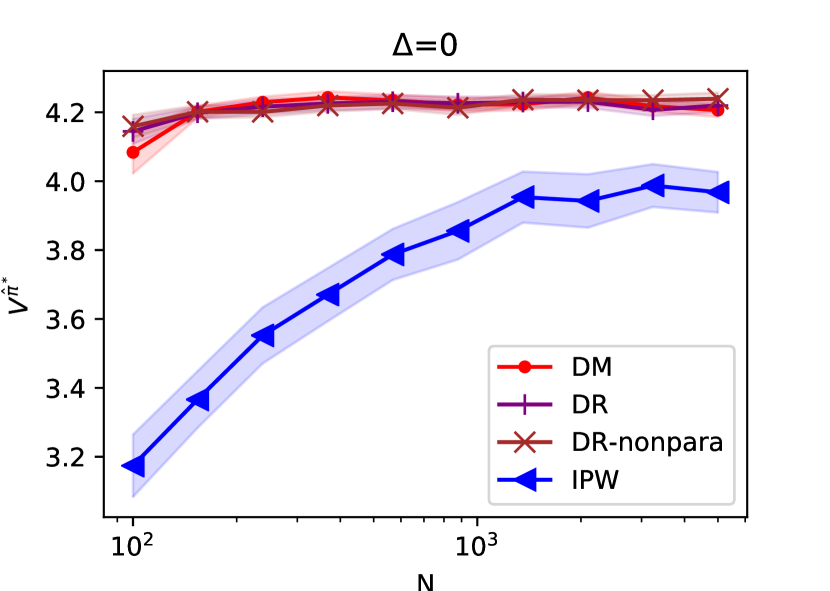
Refer to caption
(a) Out-of-sample value $V^{\hat{\pi}^{*}}$ (y-axis) of threshold policies optimized via Algorithmย 1.
Figure 4: Policy evaluation and optimization as more trajectories (x-axis) are collected of $T$-horizon selling in contextual and capacitated dynamic pricing, exampleย 1; specification of eq.ย 9.
IPW in example of Figureย 2(b)

For completeness we also include the results from the well-specified case, corresponding to $\Delta=0$ in Figureย 2(b). In the well-specified model case, model based approaches improve handily upon the high-variance $\operatorname{IPW}$ approach.

Additional strong baseline comparisons: MIS and DRL (with marginal state-action density ratios).

We also compare to state-of-the-art methods for evaluation. We emphasize that the core contribution of this approach is not in the area of off-policy evaluation itself, but rather policy optimization. Indeed, the proposal for evaluation can be understood as a special case of the backwards-recursive presentation in [28].

In this setting, we can compare to approaches which do not use the โ€œstatefulโ€ structure directly, as well as adaptations of approaches which mildly adapt to the structure. Let ฯtฯ€โ€‹(s,x)subscriptsuperscript๐œŒ๐œ‹๐‘ก๐‘ ๐‘ฅ\rho^{\pi}_{t}(s,x) be the distribution of state St=s,Xt=xformulae-sequencesubscript๐‘†๐‘ก๐‘ subscript๐‘‹๐‘ก๐‘ฅS_{t}=s,X_{t}=x when executing policy $\pi$, starting from initial state $S_{0}$ drawn from an initial distribution over states. We can correspondingly define a state-action distribution. One way to use the โ€œstatefulโ€ structure is to recognize that the finite-horizon state-action density ratio

htโ€‹(st,xt,at)=ฯtฯ€eโ€‹(st,xt,at)ฯtฯ€bโ€‹(st,xt,at)=ฯtฯ€eโ€‹(st,at)ฯtฯ€bโ€‹(st,at)โ€‹fโ€‹(xt)fโ€‹(xt)subscriptโ„Ž๐‘กsubscript๐‘ ๐‘กsubscript๐‘ฅ๐‘กsubscript๐‘Ž๐‘กsuperscriptsubscript๐œŒ๐‘กsubscript๐œ‹๐‘’subscript๐‘ ๐‘กsubscript๐‘ฅ๐‘กsubscript๐‘Ž๐‘กsuperscriptsubscript๐œŒ๐‘กsubscript๐œ‹๐‘subscript๐‘ ๐‘กsubscript๐‘ฅ๐‘กsubscript๐‘Ž๐‘กsuperscriptsubscript๐œŒ๐‘กsubscript๐œ‹๐‘’subscript๐‘ ๐‘กsubscript๐‘Ž๐‘กsuperscriptsubscript๐œŒ๐‘กsubscript๐œ‹๐‘subscript๐‘ ๐‘กsubscript๐‘Ž๐‘ก๐‘“subscript๐‘ฅ๐‘ก๐‘“subscript๐‘ฅ๐‘กh_{t}(s_{t},x_{t},a_{t})=\frac{\rho_{t}^{\pi_{e}}(s_{t},x_{t},a_{t})}{\rho_{t}^{\pi_{b}}(s_{t},x_{t},a_{t})}=\frac{\rho_{t}^{\pi_{e}}(s_{t},a_{t})}{\rho_{t}^{\pi_{b}}(s_{t},a_{t})}\frac{f(x_{t})}{f(x_{t})}

is independent of $x$ since $x$ is exogenously generated. Therefore the marginal density ratio only varies in st,atsubscript๐‘ ๐‘กsubscript๐‘Ž๐‘กs_{t},a_{t}, htโ€‹(st,at)=ฯtฯ€eโ€‹(st,at)ฯtฯ€bโ€‹(st,at)subscriptโ„Ž๐‘กsubscript๐‘ ๐‘กsubscript๐‘Ž๐‘กsuperscriptsubscript๐œŒ๐‘กsubscript๐œ‹๐‘’subscript๐‘ ๐‘กsubscript๐‘Ž๐‘กsuperscriptsubscript๐œŒ๐‘กsubscript๐œ‹๐‘subscript๐‘ ๐‘กsubscript๐‘Ž๐‘กh_{t}(s_{t},a_{t})=\frac{\rho_{t}^{\pi_{e}}(s_{t},a_{t})}{\rho_{t}^{\pi_{b}}(s_{t},a_{t})}. The corresponding marginalized importance sampling estimator of [56] is $\mathbb{E}_{N}[\sum_{t=0}^{T}h_{t}(S_{t},A_{t})R_{t}]$. With a nuisance estimate of $Q_{\pi}$, the efficient estimator of [30] is

$$\mathbb{E}_{N}\left[\sum_{t=0}^{T}h_{t}(S_{t},A_{t})(R_{t}-Q_{t}^{\pi}(S_{t},X_{t},A_{t}))-h_{t-1}(S_{t-1},A_{t-1})\mathbb{E}_{a\sim\pi_{e}}[Q_{t}(S_{t},X_{t},a)]\right].$$

We can compare to strong baseline versions of the above by encoding the structural information by restricting attention to density ratios htโ€‹(s,a)subscriptโ„Ž๐‘ก๐‘ ๐‘Žh_{t}(s,a) satisfying functional specifications that are independent of $x$. We use $Q$ functions learned by fitted Q-evaluation as nuisance estimates for the method of [30].

Larger-dimensional policy optimization comparison

With $p=5$, fix the parameters of the dgp as:

$$\mu=[1,-0.5,0.5,-1,1],\beta=[2,2,2,-2,-2],\beta_{0}=-2.$$

The outcome model and misspecified outcome model are the following:

$\displaystyle\textstyle\mu(1\mid a,x)=(1-\Delta)\sigma(\beta^{\top}x+\beta_{0}\cdot p(a))+\Delta\sigma((x_{0}^{2}-x_{3}x_{4}-x_{1}^{2})\cdot p(a)),\;e_{t}(1\mid x)={\sigma(-0.8\beta^{\top}x)}$ (36)

In Figureย 5 we repeat the comparisons of Figuresย 2(a) andย 2(b) and find similar qualitative results and comparisons as to those of Figuresย 2(a) andย 2(b). We repeat over 48 replications. Our approaches that leverage the structure enjoy finite-sample improvements from much simpler nuisance estimation. Double-robustness greatly improves finite-sample performance of unbiased IPW, though well-specification of the nuisance parameter is important. In Figureย 5(a) we see the benefits of rate-double-robustness even in the well-specified nuisance case: both doubly-robust approaches achieve improve finite sample performance for small $N$, although these benefits become comparable when $N=2000$. We report the median because the fitted-Q-evaluation results in outliers for OPE performance.

Refer to caption
(a) Policy evaluation: $\Delta=0$
Refer to caption
(b) Policy evaluation: $\Delta=0.2$
Refer to caption
(c) Out-of-sample value $V^{\hat{\pi}^{*}}$ (y-axis) of policy optimization: threshold policies optimized via Algorithmย 1. Higher is better.
Figure 5: Policy evaluation and optimization as more trajectories (x-axis) are collected of $T$-horizon selling in contextual and capacitated dynamic pricing, exampleย 1; specification of eq.ย 36.

D.2 Details on computation

  • โ€ข

    Experiments done on a MacBook Pro with 16gb RAM.

  • โ€ข

    Experiments develop a custom Gym environment [12] as well as use Numpy, Scipy, Sci-kit Learn [43].