Gradient Gibbs measures of a SOS model on Cayley trees: 4-periodic boundary laws
F. H. Haydarov, U.A. Rozikov
F. H. Haydarova,baNational University of Uzbekistan,
Tashkent, Uzbekistan.bAKFA University, 1st Deadlock 10, Kukcha Darvoza, 100095, Tashkent, Uzbekistan.haydarov_imc@mail.ru U.Rozikovc,b,dcV.I.Romanovskiy Institute of Mathematics of Uzbek Academy of Sciences;bAKFA University, 1st Deadlock 10, Kukcha Darvoza, 100095, Tashkent, Uzbekistan;dFaculty of Mathematics, National University of Uzbekistan.rozikovu@yandex.ru
Abstract.
For SOS (solid-on-solid) model with external field and with spin values from the set of all integers,
on a Cayley tree we give gradient Gibbs measures (GGMs).
Such a measure corresponds to a boundary law (a function defined on vertices of Cayley tree)
satisfying an infinite system of functional equations.
We give several concrete GGMs which correspond to periodic boundary laws.
The study of random field from a lattice graph (usually
or a Cayley tree ) to a measure space is a
central component of ergodic theory and statistical physics.
In many classical models
from physics (e.g., the Ising model, the Potts model), is a finite set (i.e., with a finite underlying measure ), and
has a physical interpretation as the spin of a particle
at location in a crystal lattice.
Following [1], [2], [6], [7], [8], [9], [10], [11], [14], [15], let us
give basic definitions and some known facts related to (gradient) Gibbs measures.
-algebra, Hamiltonian.
In general, is a space with an infinite underlying measure (i.e. with counting measure),
where is the Borel -algebra of and usually
has a physical interpretation as the spatial position of a particle at location
in a lattice. In [6] first such models were considered.
The prime examples of unbounded spin systems are harmonic
oscillators. Another example is the Ginzburg-Landau
interface model; which is obtained from the harmonic oscillators [7], [14].
Denote by the set of functions from to , such a function also is called a configuration.
Assume random field on given as the projection onto the coordinate :
For , denote by
the smallest -algebra with respect to which is measurable for all . Write .
A subset of ,
is called a cylinder set if it belongs to for some finite set .
Let be the smallest
-algebra on containing the cylinder sets.
Write for the tail--algebra, i.e., intersection of
over all finite subsets of the sets in are called tail-measurable sets.
Assume that we are given a family of measurable potential
functions (one for each finite subset of )
each is
measurable.
For each finite subset of define a Hamiltonian:
where the sum is taken over finite subsets .
Gibbs Measures.
To define Gibbs measures and gradient Gibbs measures, we will need some additional
notation [7], [14].
Let and be general measure spaces.
A function is called a probability kernel from to if
1.
is a probability measure on for each fixed , and
2.
is -measurable for each fixed .
Such a kernel maps each measure , on to a measure on by
The following is a probability kernel from to :
where is a counting measure.
A configuration has finite energy if for all finite . Moreover, is -admissible
if each is finite and non-zero.
Given a measure on , define a new
measure by
Definition 1.
A probability measure on is called a Gibbs measure if is supported on the set of -admissible configurations in and for all finite subset we have
Gradient Gibbs measure. For any configuration and edge of
the difference along the edge is given by and is called the gradient field of .
The gradient spin variables are now defined by for each .
The space of gradient configurations denoted by . The measurable structure on the space is given by -algebra
Note that is the subset of
containing those sets that are invariant under translations for .
Similarly, we define
Let be a translation invariant
gradient potential. Since, given any , the kernels are -measurable
functions of , it follows that the kernel sends a given measure on to another
measure on .
Definition 2.
A measure on is called a gradient Gibbs measure
if for all finite subset we have
Note that, if is a Gibbs measure on , then its restriction to is a gradient
Gibbs measure.
A gradient Gibbs measure is said to be localized or smooth if it arises
as the restriction of a Gibbs measure in this way. Otherwise, it is non-localized or
rough.
It is known[7], [5, Theorem 8.19.] that
many natural Gibbs measures on are rough when .
Construction of gradient Gibbs measure on Cayley trees. Following [11]
we consider models where spin-configuration is a function from the
vertices of the Cayley tree to the set , where
is the set of vertices and is the set of oriented edges (bonds) of the tree
(see Chapter 1 of [13] for properties of the Cayley tree).
For nearest-neighboring (n.n.) interaction potential , where
is an edge, define symmetric transfer matrices by
(1.1)
where is the set of all nearest-neighbors of and denotes the number of elements of the set .
Define the Markov (Gibbsian) specification as
If for any bond the transfer operator is
a function of gradient spin variable then the underlying potential is called
a gradient interaction potential.
Boundary laws (see [15]) which allow to describe the set of all Gibbs measures (that are Markov chains on trees).
Definition 3.
A family of vectors with is called a boundary law for the transfer operators if for each there exists a constant such that the consistency equation
(1.2)
holds for every .
A boundary law is called -periodic if for every oriented edge and each .
It is known that there is a one-to-one correspondence between boundary laws
and tree-indexed Markov chains if the boundary laws are normalisable in the sense of Zachary [15]:
Definition 4.
A boundary law is said to be normalisable if and only if
(1.3)
at any .
For any we define its outer boundary as
The correspondence now reads the following:
Theorem 1.
[15]
For any Markov specification with associated family of transfer matrices we have
(1)
Each normalisable boundary law for defines a unique tree-indexed Markov chain via the equation given for any connected set
(1.4)
where for any , denotes the unique of in .
(2)
Conversely, every tree-indexed Markov chain admits a representation of the form (1.4) in terms of a normalisable boundary law (unique up to a constant positive factor).
The Markov chain defined in (1.4) has the transition probabilities
(1.5)
The expressions (1.5) may exist even in situations where the underlying boundary
law is not normalisable. However, the Markov chain given by (1.5), in general, does not have an invariant probability measure.
Therefore in [8], [9], [10], [11]
some non-normalisable boundary laws are used to give gradient Gibbs measures.
Now we give some results of above mentioned papers. Consider a model on Cayley tree , where the spin takes values in
the set of all integer numbers . The set of all configurations is .
For , fix a site . If the boundary law is assumed to be -periodic, then take and define probability measure on by
where is a normalization constant, is the unique path from to
and denotes the coset projection.
Theorem 2.
[11]
Let be any
-periodic boundary law to some gradient interaction potential.
Fix any site and any class label . Then
(1.6)
gives a consistent family of probability measures on the gradient space .
Here with is any finite connected set,
and is a normalization constant.
The measures will be called pinned gradient measures.
If -periodic boundary law and the underlying potential are translation invariant then it is possible to obtain
probability measure on the gradient space by mixing the pinned gradient measures:
Theorem 3.
[11] Let a -periodic boundary law and its gradient interaction potential are translation invariant.
Let be any finite connected set and let be any vertex. Then the measure with marginals given by
(1.7)
where is a normalisation constant, defines a translation invariant gradient Gibbs measure on .
SOS model. The (formal) Hamiltonian of the SOS model is
(1.8)
where is a constant.
In [8], using Theorem 3 some gradient Gibbs measures are found.
Let be inverse temperature and .
The transfer operator then reads for any ,
and a translation invariant boundary law, denoted by , is any positive function on
solving the consistency equation, whose values we will denote by instead of .
By definition of the boundary law it is only unique up to multiplication with any positive prefactor.
Hence we may choose this constant in a way such that we have .
Set . Then the boundary law equation (for translation-invariant case, i.e.
, for all ) reads
[8] If (i.e. ) then the equation (1.9) is equivalent to the following
(1.10)
where .
In general, solutions of (1.10) are not known. But in class of periodic solutions, some results are obtained.
The following theorem is proved for and -periodic boundary laws:
Theorem 4.
[8] For the SOS model (1.8) on the binary tree (i.e. ) with parameter the following assertions hold
1.
If then there is precisely one GGM associated to a 4-periodic boundary law.
2.
If then there are precisely two GGMs.
3.
If then there are precisely three GGMs.
4.
If then there are precisely four such measures.
The following theorem is proved for any and -periodic boundary laws.
Denote
Theorem 5.
[8] For the SOS-model on the -regular tree, , with parameter there is such that
and the following holds:
1.
If then there is no any GGM corresponding to
a nontrivial 3-periodic boundary.
2.
At there is a unique GGM corresponding to a
nontrivial -periodic boundary law.
3.
For , (resp. ) there are exactly
two such (resp. one) GGMs.
The GGMs described above are all different from the GGMs mentioned in Theorem 4.
General case.
Assume that the transfer operator , defined in (1.1), is summable, i.e.
For any summable and any degree there is a finite period
such that for all there are GGMs of
period which are not translation invariant.
Moreover, in [10] the authors provided general conditions in terms of the
relevant -norms of the associated transfer operator which ensure the existence of
a countable family of proper Gibbs measures. The existence of delocalized GGMs is proved, under natural conditions on .
This implies coexistence of both types of measures for large classes of models including the SOS-model,
and heavy-tailed models arising for instance for potentials of logarithmic growth.
2. 4-periodic boundary laws for
In this section our goal is to find solutions of (1.10) which have the form
(2.1)
where and some positive numbers.
Then from (1.10) for and we get the following system of equations
(2.2)
The case is fully analyzed in [8] and the following is proved
Proposition 2.
For the periodic solutions of the form (2.1) (i.e. solutions of the system (2.2))
depend on the parameter in the following way.
(1)
If then there is a unique solution.
(2)
If then there are exactly two solutions.
(3)
If then there are exactly four solutions.
(4)
If then there are exactly five solutions.
where explicit formula of each solution is found.
Now we reduce the system (2.2) to a polynomial equation with one unknown . To do this
from the first (resp. second) equation of (2.2) find (resp. ):
The last polynomial equation has exactly one positive solution,
because signs of its coefficients changed only one time,
and at it is negative, i.e. -1 and at it is positive.
Moreover, this unique solution is , because putting in (2.7) we get
Thus has unique minimum
at , and .
Consequently,
These properties of completes the proof.
∎
Remark 1.
The equation (2.6) was also considered in [3].
Lemma 1 improves their result (see Theorem 5.2 of [3]), because we found explicit
formula for the critical value .
Now we want to find solutions of (2.4) which are different from solutions of (i.e., ).
By simple calculations the equation (2.4) can be rewritten as
(2.8)
Recall that divides . Now we shall find .
It is easy to see that can be written as
Consequently, the equation (2.4) in case is reduced to
(2.9)
But may have some roots coinciding with roots of . This is result of the following lemma.
Lemma 2.
Let be a root of . Then is a root of iff
and satisfies
(2.10)
Proof.
For the root we have . Therefore from (2.9), i.e. , we get
By Lemma 1 we know that has a solution different
from 1 iff . Therefore .
The polynomial equation (2.11) has exactly one positive solution, denoted by ,
because signs of its coefficients changed only one time. Moreover, we have , because at the LHS of (2.11) is negative:
and at it is positive. Thus .
∎
Example 1.
For we have
Remark 2.
It seems impossible to solve equation (2.9) for each . But one can use numerical
methods to give some its solutions for concrete values of parameters.
Therefore, one can try to solve it for small values of . In [8] the case is fully analyzed.
Below we shall consider the case . Cases remains open.
Case . In this case the equation (2.9) has the form
(2.12)
It is well known (see [12], p.28) that the number of positive
roots of the polynomial (2.12) does not exceed the number of sign
changes of its coefficients.
Since , the number of positive roots of
the polynomial (2.12) is at most . Numerical analysis shows that
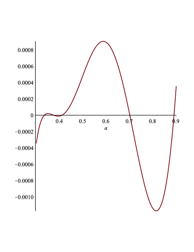
for some values of there are exactly 6 solutions (see Fig.1).
Indeed, rewrite (2.12) as
Note that, for fixed , the function is continuous with respect
to both arguments , and is a bounded function.
Moreover, and .
Figure 1. Graph of function , for and . Hence, has 6 (the maximal number) positive solutions.
Remark 3.
For one can explicitly find all positive solutions of (2.5), i.e.
Moreover, .
In case , we do not know explicit solutions of (2.12).
Since may be negative for some positive solutions ,
we have to check positivity of for each positive . To avoid this difficulty, in case and , we solve (2.2) as
follows.
We rewrite the system of equations (2.2) for the case .
(2.13)
Lemma 4.
For the system (2.13) there are critical
values and of such that the following assertions hold
(1)
If then there is no any solution.
(2)
If then there is precisely one solution.
(3)
If then there are precisely two solution to (2.13).
Proof.
We add the first and second equations of (2.13), i.e.,
If then there is one solution to (2.13), i.e., . We have to find solutions, so we can suppose . Consequently,
From the last equality, one gets
(2.14)
Now, we subtract the second equation of (2.13) from the first one. Then
Since , both sides can be divided by and we obtain the following
By Ferrari’s method for solving a quartic equation, the equation (2.16) can be written as
(2.17)
where is a real root of the following polynomial
Denote
To find a certain view of , we shall find a real root of . By Cardano’s formula, roots of are:
where
It’s known that the expression is called the discriminant of the equation.
•
If , then one root is real and two are complex conjugates.
•
If , then all roots are real, and at least two are equal.
•
If , then all roots are real and unequal.
We have
Note that there are two positive solutions of on i.e., and and for and for
For all cases, is a real solution and we can choose as . In addition, .
The equation (2.17) can be written as
Hence, we have only two cases . When (resp ) belongs to the interval then (resp. ) is also positive. Again we use numerical analysis and obtain the following results: if then , i.e., the equation has no any positive solution such that . Also, for all we have , i.e., the equation has exactly one positive solution with . Let , then and in this case the equation has exactly two positive solutions with , where .
∎
Denote by the number of positive roots of (2.13).
Then (for ) by Lemma 1 (where ), Lemma 3, Lemma 4
we obtain the following formula
(2.18)
where , .
In [8] some statements on identifiability of GGM with respect to the class of boundary laws are proven.
In particular, for 4-periodic case the following is known.
Lemma 5.
[8] Consider any 4-periodic boundary law constructed by given in (2.1)
and denote the associated GGM by . Let be two such boundary laws. If then necessarily
Based on formula (2.18), Remark 3 and Lemma 5 we conclude the following
Theorem 7.
For the SOS model (1.8) on the Cayley tree of order
there are critical values , such that the following assertions hold
(1)
If then there is precisely one GGM associated to a boundary law of the type (2.1).
(2)
If then there are precisely two such GGMs.
(3)
If then there are at most three such GGMs.
(4)
If then there are at
most four such measures associated to boundary laws of the type (2.1).
3. SOS model with an external field
3.1. The boundary law equation in case of non-zero external field.
In this section for , consider Hamiltonian
of SOS model with external field , i.e.,
Denote , .
Then the equation for translation-invariant boundary laws has the following form
(3.1)
Note that this equation coincides with (1.9) for .
In this case there is only one positive real solution. It is
Case:
In this case there are two positive real solutions. These roots are
Case:
In this case and there are three positive real solutions:
Proof.
The conditions of existence of real solutions are well-known111https://en.wikipedia.org/wiki/Cubic-equation. The positivity of each solution follows from Lemma 7.
∎
Case .
In this case from the second equation of (3.7) we get
Note that this equation has only positive real solutions.
Moreover, one can see that if
then the quadratic equation has the following positive solutions
Using (3.8) we get and . Clearly all of these solutions are positive.
Denote by the gradient Gibbs measure corresponding to solution , .
Thus depending on the values related to and sets , we have the following result.
Theorem 8.
For the SOS model with 4-periodic external field there are up to seven 4-periodic gradient Gibbs measures , .
Acknowledgements
The author thanks C. Külske for helpful discussions.
References
[1] M. Biskup, R. Kotecký, Phase coexistence of gradient Gibbs states, Probab. Theory Related Fields 139(1-2) (2007), 1–39.
[2] R. Bissacot, E.O. Endo, A.C.D. van Enter, Stability of the phase transition of critical-field Ising model on Cayley trees under inhomogeneous external fields, Stoch. Process. Appl. 127(12) (2017), 4126–4138.
[3] G.I. Botirov, F.H. Haydarov, Gradient Gibbs measures for the SOS model with integer spin values on a Cayley tree. J. Stat. Mech. Theory Exp. 9 (2020), 093102, 9 pp.
[4]
A.C.D. van Enter, C.Külske, Non-existence of random gradient Gibbs measures in continuous interface models in , Ann. Appl. Probab. 18 (2008) 109–119.
[5] S. Friedli, Y. Velenik, Statistical mechanics of lattice systems. A concrete mathematical introduction. Cambridge University Press, Cambridge, 2018. xix+622 pp.
[6] T. Funaki, H. Spohn, Motion by mean curvature from the Ginzburg-Landau interface model, Comm. Math. Phys., 185, 1997.
[7] H.O. Georgii, Gibbs Measures and Phase Transitions, Second edition. de Gruyter Studies in Mathematics, 9. Walter de Gruyter, Berlin, 2011.
[8] F. Henning, C. Külske, A. Le Ny, U.A. Rozikov, Gradient Gibbs measures for the SOS model with countable values on a Cayley tree. Electron. J. Probab. 24 (2019), Paper No. 104, 23 pp.
[9] F. Henning, C. Külske, Existence of gradient Gibbs measures on regular trees which are not translation invariant. arXiv:2102.11899 [math.PR]
[10] F. Henning, C. Külske, Coexistence of localized Gibbs measures and delocalized gradient Gibbs measures on trees. arXiv:2002.09363 [math.PR]
[11] C. Külske, P. Schriever. Gradient Gibbs measures and fuzzy transformations on trees, Markov Process. Relat. Fields 23, (2017), 553-590.
[13] U.A. Rozikov, Gibbs measures on Cayley trees. World Sci. Publ. Singapore. 2013.
[14] S. Sheffield, Random surfaces: Large deviations principles and gradient Gibbs measure classifications.
Thesis (Ph.D.)-Stanford University. 2003. 205 pp.
[15] S. Zachary, Countable state space Markov random fields and Markov chains on trees, Ann. Probab. 11(4) (1983), 894–903.