Abstract

Random Forests (RF) are among the state-of-the-art in many machine learning applications. With the ongoing integration of ML models into everyday life, the deployment and continuous application of models becomes more and more an important issue. Hence, small models which offer good predictive performance but use small amounts of memory are required. Ensemble pruning is a standard technique to remove unnecessary classifiers from an ensemble to reduce the overall resource consumption and sometimes even improve the performance of the original ensemble. In this paper, we revisit ensemble pruning in the context of ‘modernly’ trained Random Forests where trees are very large. We show that the improvement effects of pruning diminishes for ensembles of large trees but that pruning has an overall better accuracy-memory trade-off than RF. However, pruning does not offer fine-grained control over this trade-off because it removes entire trees from the ensemble. To further improve the accuracy-memory trade-off we present a simple, yet surprisingly effective algorithm that refines the predictions in the leaf nodes in the forest via stochastic gradient descent. We evaluate our method against 7 state-of-the-art pruning methods and show that our method outperforms the other methods on 11 of 16 datasets with a statistically significant better accuracy-memory trade-off compared to most methods. We conclude our experimental evaluation with a case study showing that our method can be applied in a real-world setting.

1 Introduction

Ensemble algorithms offer state-of-the-art performance in many applications and often outperform single classifiers by a large margin. With the ongoing integration of embedded systems and machine learning models into our everyday life, e.g in the form of the Internet of Things, the hardware platforms which execute ensembles must also be taken into account when training ensembles.

From a hardware perspective, a small ensemble with minimal execution time and a small memory footprint is desired. Similar, learning theory indicates that ensembles of small models should generalize better which would make them ideal candidates for small, resource constraint devicesKoltchinskii et al. (2002); Cortes et al. (2014). Practical problems, on the other hand, often require ensembles of complex base learners to achieve good results. For some ensembling techniques such as Random Forest it is even desired that individual trees are as large as possible leading to overall large ensembles Breiman (2000); Biau (2012); Denil et al. (2014); Biau & Scornet (2016). Ensemble pruning is a standard technique for implementing ensembles on small devices Tsoumakas et al. (2009); Zhang et al. (2006) by removing unnecessary classifiers from the ensemble. Remarkably, this removal can sometimes lead to a better predictive performance Margineantu & Dietterich (1997); Martínez-Muñoz & Suárez (2006); Li et al. (2012). In this paper, we revisit ensemble pruning and show that this improvement effect does not carry over to the modern-style of training individual trees as large as possible in Random Forests. Maybe even more frustrating, ensemble pruning does not seem to be necessary anymore to achieve the best accuracy if the original forest has a sufficient amount of large trees. If, however, one also considers the memory requirements of the individual trees the situation changes. We argue that, from a hardware perspective, the trade-off between memory and accuracy is what really matters. Although a Random Forest might produce a good model it might not be possible to deploy it onto a small device due to its memory requirements. As shown later, the best performing RF models are often larger than $5-10$ MB (see e.g. Fig. 2 and Fig. 3) while most available microcontroller units (MCU) only offer a few KB to a few MB of memory as depicted in Table 1. Hence, to deploy RF onto these small devices we require a good algorithm which gives accurate models for a variety of different memory constraints.

MCU	Flash	(S)RAM	Power
Arduino Uno	32KB	2KB	12mA
Arduino Mega	256KB	8KB	6mA
Arduino Nano	26–32KB	1–2KB	6mA
STM32L0	192KB	20KB	7mA
Arduino MKR1000	256KB	32KB	4mA
Arduino Due	512KB	96KB	50mA
STM32F2	1MB	128KB	21mA
STM32F4	2MB	384KB	50mA

Table 1: Available memory on different microcontroller units. Excerpt from Branco et al. (2019).

We directly optimize the accuracy-memory trade-off by introducing a technique called leaf-refinement. Leaf-Refinement is a simple, but surprisingly effective method, which, instead of removing trees from the ensemble, further refines the predictions of small ensembles using gradient-descent. This way, we can refine any given tree-ensemble to optimize its accuracy thereby maximizing the accuracy-memory trade-off. Our contributions are as follows:

• Revisiting ensemble pruning: We revisit ensemble pruning in the context of modernly trained Random Forests in which individual trees are typically large. We show that pruning a Random Forest can improve the accuracy if individual trees are small, but this effect becomes neglectable for larger trees. Moreover, if we are only interested in the most accurate models where memory is no constraint we can simply train unpruned Random Forests which yields comparable results without the need for pruning.

• Random Forest with Leaf Refinement: We show that pruning exhibits a better accuracy-memory trade-off than RF does. To further optimize this trade-off we present a simple, yet surprisingly effective gradient-descent based algorithm called leaf-refinement (RF-LR) which refines the predictions of a pre-trained Random Forest.

• Experiments: We show the performance of our algorithm on 16 datasets and compare it against 7 state-of-the-art pruning methods. We show that RF-LR outperforms the other methods on 11 of 16 datasets with a statistically significant better accuracy-memory trade-off compared to most methods. We conclude our experimental evaluation with a case study showing that our method can be applied on a real-world setting.

The paper is organized as the following. Section 2 presents our notation and related work. In Section 3 we revisit ensemble pruning in the context of ‘modern’ Random Forests, whereas section 4 discusses how to improve the accuracy-memory trade-off without ensemble pruning. In section 5 we experimentally evaluate our method and in section 6 we conclude the paper.

2 Background and Notation

We consider a supervised learning setting, in which we assume that training and test points are drawn i.i.d. according to some distribution $\mathcal{D}$ over the input space $\mathcal{X}$ and labels $\mathcal{Y}$. We assume that we have given a trained ensemble with $M$ classifiers $h_{i}\in\mathcal{H}$ of the following form:

$$f(x)=\frac{1}{M}\sum_{i=1}^{M}h_{i}(x)$$ (1)

Additionally, we have given a labeled pruning sample $\mathcal{S}=\{(x_{i},y_{i})|i=1,\dots,N\}$ where $x_{i}\in\mathcal{X}\subseteq\mathbb{R}^{d}$ is a $d$-dimensional feature-vector and $y_{i}\in\mathcal{Y}\subseteq\mathbb{R}^{C}$ is the corresponding target vector. This sample can either be the original training data used to train $f$ or another pruning set not related to the training or test data. For classification problems with $C\geq 2$ classes we encode each label as a one-hot vector $y=(0,\dots,0,1,0,\dots,0)$ which contains a ‘$1$’ at coordinate $c$ for label $c\in\{0,\dots,C-1\}$; for regression problems we have $C=1$ and $\mathcal{Y}=\mathbb{R}$. In this paper, we will focus on classification problems, but note that our approach is directly applicable for regression tasks, as well. Moreover we will focus on tree ensembles and specifically Random Forests, but note that most of our discussion directly translates to other tree ensembles such as Bagging Breiman (1996), ExtraTrees Geurts et al. (2006), Random Subspaces Ho (1998) or Random Patches Louppe & Geurts (2012).

The goal of ensemble pruning is to select a subset of $K$ classifier from $f$ which forms a small and accurate sub-ensemble. Formally, each classifier $h_{i}$ receives a corresponding pruning weight $w_{i}\in\{0,1\}$. Let

$$L(w)=\frac{1}{N}\sum_{(x,y)\in\mathcal{S}}\ell\left(\sum_{i=1}^{M}w_{i}h_{i}(x),y\right)$$ (2)

be a loss function and let $\lVert w\rVert_{0}=\sum_{i=1}^{M}1\{w_{i}>0\}$ be the $l_{0}$ norm which counts the number of nonzero entries in the weight vector $w=(w_{1},w_{2},\dots,w_{M})$. Then the ensemble pruning problem is defined as:

$$\arg\min_{w\in\{0,1\}^{M}}L(w)\text{~{}st.~{}}\lVert w\rVert_{0}=K$$ (3)

Many effective ensemble pruning methods have been proposed in literature. These methods usually differ in the specific loss function used to measure the performance of a sub-ensemble and the way this loss is minimized. Tsoumakas et al. give in Tsoumakas et al. (2009) a detailed taxonomy of pruning methods which was later expanded in Zhou (2012) to which we refer interested readers. Early works on ensemble pruning focus on ranking-based approaches which assign a rank to each classifier depending on their individual performance and then pick the top $K$ classifier from to the ranking. One of the first pruning methods in this direction was due to Margineantu and Dietterich which proposed to use the Cohen-Kappa statistic to rate the effectiveness of each classifier in Margineantu & Dietterich (1997). More recent approaches also incorporate the ensemble’s diversity into the selection such as Lu et al. (2010); Jiang et al. (2017); Guo et al. (2018). As an alternative to a simple ranking, Mixed Quadratic Integer Programming (MQIP) has also been proposed. Originally this approach was proposed by Zhang et al. in Zhang et al. (2006) which uses the pairwise errors of each classifier to formulate an MQIP. Cavalcanti et al. expand on this idea in Cavalcanti et al. (2016) which combines 5 different measures into the MQIP. A third branch of pruning considers the clustering of ensemble members to promote diversity. The main idea is to cluster the classifiers into (diverse) groups and then to select one representative from each group Giacinto et al. (2000); Lazarevic & Obradovic (2001). Last, ordering-based pruning has been proposed. Ordering-based approaches order all ensemble members according to their overall contribution to the (sub-)ensemble and then pick the top $K$ classifier from this list. This approach was also first considered in Margineantu & Dietterich (1997) which proposed to greedily minimize the overall ensemble error. A series of works by Martínez-Muñoz, Suárez and others Martınez-Munoz & Suárez (2004); Martínez-Muñoz & Suárez (2006); Martínez-Muñoz et al. (2008) add upon this work proposing different error measures. More recently, theoretical insights from PAC theory and the bias-variance decomposition were also transformed into greedy pruning approaches Li et al. (2012); Jiang et al. (2017).

Looking beyond ensemble pruning there are numerous, orthogonal methods to deploy ensembles to small devices. First, ‘classic’ decision tree pruning algorithms (e.g. minimal cost complexity pruning or sample complexity pruning) already reduce the size of DTs while offering a better accuracy (c.f. Barros et al. (2015)). Second, in the context of model compression (see e.g. Choudhary et al. (2020) for an overview) specific models such as Bonsai Kumar et al. (2017) or Decision Jungles Shotton et al. (2013) aim to find smaller tree ensembles already during training. Last, the optimal implementation of tree ensembles has also been studied, e.g. by optimizing the memory layout for caching Buschjäger et al. (2018) or changing the tree traversal to utilize SIMD instructions Ye et al. (2018). We find that all these methods are orthogonal to our approach and that they can be freely combined with one another, e.g. we may train a decision jungle, then perform ensemble pruning or leaf-refinement on it and finally find the optimal memory layout of the trees in the jungle for the best deployment.

3 Revisiting Ensemble Pruning

Before we discuss our method we first want to revisit Reduced Error Pruning (RE, Margineantu & Dietterich (1997)) and repeat some experiments performed with it. RE pruning is arguably one of the simplest pruning algorithms but often offers competitive performance. RE is a ordering-based pruning method. It starts with an empty ensemble and iteratively adds that tree which minimizes the overall ensemble error the most until $K$ members have been selected. Algorithm 1 depicts this approach where $L$ is the $0-1$ loss and $e_{i}$ denotes the unit vector with a ‘1’ entry at position $i$.

1:  $w\leftarrow(0,\dots,0)$

2:  $i\leftarrow\arg\min\{L(w+\vec{e}_{i})|i=1\dots,M\}$

3:  $w\leftarrow w+\vec{e}_{i}$

4:  for $j=1,\dots,K-1$ do

5:     $i\leftarrow\arg\min\{L(w+\vec{e}_{i})|i=1\dots,M,w_{i}\not=1\}$

6:     $w\leftarrow w+\vec{e}_{i}$

7:  end for

Algorithm 1 Reduced Error Pruning (RE).

We will now perform experiments in the spirit of Martínez-Muñoz & Suárez (2006), but adapt a more modern approach to training the base ensembles. In the original experiments, the authors show that when pruning a Bagging Ensemble of 200 pruned CART trees, that RE (among other methods) achieves a better accuracy with fewer trees compared to the original ensemble. This result has been empirically reproduced in various contexts (see e.g. Margineantu & Dietterich (1997); Zhou et al. (2002); Zhou (2012)) and has been formalized in the Many-Could-Be-Better-Than-All-Theorem Zhou et al. (2002). It shows that the error of an ensemble excluding the $k-$th classifier can be smaller than the error of the original ensemble if the bias $C_{k,k}$ is larger than its variance wrt. to the ensemble:

$$\sum_{i=1,i\not=k}^{M}\sum_{j=1,i\not=k}^{M}\frac{C_{i,j}}{(M-1)^{2}} \leq\sum_{i=1}^{M}\sum_{h=1}^{M}\frac{C_{i,j}}{M^{2}}$$ (4)

$$\Leftrightarrow\quad-2\sum_{i=1,i\not=k}^{M}C_{i,k} \leq C_{k,k}$$ (5)

where

$$C_{k,k} =\mathbb{E}_{x,y\sim\mathcal{D}}\left[(h_{k}(x)-y)^{2}\right]$$ (6)

$$C_{k,i} =\mathbb{E}_{x,y\sim\mathcal{D}}\left[(h_{k}(x)-y)(h_{i}(x)-y)\right]$$ (7)

Recall that the bias of a DT rapidly decreases while the variance increases wrt. to the size of the tree Domingos (2000). The original experiment used pruned decision trees whereas the today’s accepted standard is to train trees as large as possible for minimal errors (see Breiman (2000); Biau (2012); Denil et al. (2014); Biau & Scornet (2016) for more formal arguments on this). Hence, it is conceivable that ensemble pruning does not have the same beneficial effect on ‘modern’ Random Forests compared to RF-like ensembles trained 20 years ago. We will now investigate this hypothesis experimentally. As an example we will consider the EEG dataset which has $14~{}980$ datapoints with $14$ attributes and two classes (details for each dataset can be found in the appendix). By today’s standards this dataset is small to medium size which allows us to quickly train and evaluate different configurations but it is roughly two times larger than the biggest dataset used in original experiments. We perform experiments as follows: Oshiro et al. showed in Oshiro et al. (2012) empirically on a variety of datasets that the prediction of a RF stabilizes between $128$ and $256$ trees and adding more trees to the ensemble does not yield significantly better results. Hence, we train the ‘base’ Random Forests with $M=256$ trees. To control the individual errors of trees we set the maximum number of leaf nodes $n_{l}$ to values between $n_{l}\in\{64,128,256,512,1024\}$. For ensemble pruning we use RE which is tasked to select $K\in\{2,4,8,16,32,64,128,256\}$ trees from the original RF. We compare this against a smaller RF with $K\in\{2,4,8,16,32,64,128,256\}$ trees, so that we recover the original RF for $K=M=256$ on both cases. For RE we use the training data as pruning set. Experiments with a dedicated pruning set can be found in the appendix. Figure 1 shows the average accuracy over the size of the ensemble for a $5$-fold cross-validation. The dashed lines depict the smaller RF and solid lines are the corresponding pruned ensemble. As expected, we find that ensemble pruning significantly improves the accuracy when smaller trees with $64-256$ leaf nodes are used. Moreover, the performance of the pruned forests approaches the performance of the original forests when more and more trees are added much like in the original experiments. However, the improvement in accuracy becomes negligible for trees with up to $1024$ leaf nodes. Here, the accuracy of the pruned and the unpruned forest are near identical for any given number of trees. Maybe even worse, if we are only interested in the most accurate model then there is no reason to prune the ensemble as an unpruned Random Forest already seems to achieves the best performance.

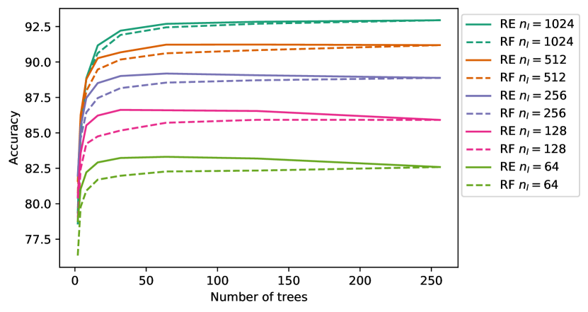
Figure 1: 5-fold cross-validation accuracy over the number of members in the ensemble for different $n_{l}$ parameters on the EEG dataset. Dashed lines depict the small RF and solid lines are the pruned ensemble via Reduced Error pruning. Best viewed in color.

We acknowledge that this experiment is one-sided because we only use Reduced Error Pruning – a nearly 25 year old method – for comparison. Maybe the problem simply lies in RE itself and not pruning in general? To verify this hypothesis we also repeated the above experiment with 6 additional pruning algorithms from the three different categories. In total we compare two ranking-based methods namely IE Jiang et al. (2017) and IC Lu et al. (2010); the three ordering-based methods RE Margineantu & Dietterich (1997), DREP Li et al. (2012) and COMP Martınez-Munoz & Suárez (2004) and the two clustering-based pruning CA Lazarevic & Obradovic (2001) and LMD Giacinto et al. (2000). We also experimented with MQIP pruning methods Zhang et al. (2006); Cavalcanti et al. (2016), but unfortunately the MQIP solver (in our case Gurobi) used during experiments would frequently fail or time-out. Thus we decided to not include any MQIP pruning methods in our evaluation.

$n_{l}$	K	COMP	DREP	IC	IE	LMD	RE	RF
64	8	81.86	80.79	81.71	81.34	81.46	82.22	80.92
	32	83.09	82.33	83.10	82.22	82.60	83.23	81.98
	128	83.17	82.38	83.10	82.49	82.87	83.19	82.34
128	8	85.12	84.08	84.69	84.81	83.85	85.53	84.23
	32	86.34	85.49	86.38	85.76	85.65	86.62	85.17
	128	86.40	85.75	86.27	86.00	86.03	86.54	85.92
256	8	87.37	86.24	87.14	87.16	86.36	87.46	86.44
	32	88.97	88.02	89.07	88.70	88.37	89.01	88.16
	128	88.97	88.70	89.15	88.97	88.77	89.07	88.71
512	8	88.36	88.51	88.96	88.78	87.44	88.79	87.95
	32	91.11	90.30	91.34	90.67	90.37	90.68	90.17
	128	91.22	90.91	91.41	91.30	90.87	91.23	90.83
1024	8	89.45	89.26	89.51	89.70	88.30	88.85	88.83
	32	92.25	92.30	92.64	92.60	91.82	92.21	91.91
	128	92.85	92.85	93.17	92.98	92.70	92.84	92.70

Table 2: 5-fold cross-validation accuracy over the number of members $K\in\{8,32,128\}$ in the ensemble for different $n_{l}$ parameters and different methods on the EEG dataset. Rounded to the second decimal digit. Larger is better. The best method is depicted in bold.

Table 2 shows the result of this experiment. For space reasons we only depict results for $K\in\{8,32,128\}$. As expected, all pruning methods manage to improve the performance of the original RF for smaller $n_{l}\leq 256$ and keep this advantage to some degree for larger $n_{l}$. However, this advantage becomes smaller and smaller for larger $n_{l}$ until it is virtually non-existent for $n_{l}=1024$ and the accuracies are near identical. Again, as expected setting $n_{l}$ to larger values leads to the overall best accuracy.

For presentational purposes we highlighted this experiment on the EEG dataset, but we found that this behavior seems to hold universally across the other 15 datasets we experimented with. The detailed results for these experiments are given in the appendix. While the specific curves would differ we always found that the performance of a well-trained forest and its pruned counterpart would nearly match once the individual trees become large enough. For more plots with experiments on other datasets and other ‘base’ ensembles please consult the appendix.

4 Improving the accuracy-memory trade-off of RF

Clearly, the previous section shows that we cannot expect the accuracy of a pruned forest to improve much upon the performance of a well-trained Random Forest. On the one hand, this is a clear argument in favor of Random Forests – why should we prune a pre-trained forest if we can directly train a similar forest in the first place? On the other hand, pruning shows clear superior performance for smaller $n_{l}$ compared to RF. While pruning and RF both converge against a very similar maximum accuracy, pruning shows a better trade-off between the model size (controlled by $n_{l}$ and $K$) and the accuracy.

We argue that, from a hardware perspective, this trade-off is what really matters and a good algorithm should produce accurate models for a variety of different model sizes. Ensemble pruning improves this trade-off by removing unnecessary trees from the ensemble thereby reducing the memory consumption while keeping (or improving) its predictive power. But, the removal of entire trees does not offer a very fine-grained control over this trade-off. For example, it could be better to train a large forest with many, but comparably small trees instead of having one small forest of large trees. Hence, we propose to directly evaluate the accuracy-memory trade-off and to optimize towards it.

To do so, we present a simply and surprisingly effective method which refines the predictions of a given forest with Stochastic Gradient Descent (SGD). Our method trains a small initial Random Forest (e.g. by using small values for $n_{l}$ and $M$) and then refines the predictions of the individual trees to improve the overall performance: Recall that DTs use a series of axis-aligned splits of the form $\mathbbm{1}\{x_{i}\leq t\}$ and $\mathbbm{1}\{x_{i}>t\}$ where $i$ is a pre-computed feature index and $t$ is a pre-computed threshold to determine the leaf nodes. Let $s_{l}(x)\colon\mathcal{X}\to\{0,1\}$ be the series of splits which is ‘1’ if $x$ belongs to leaf $l$ and ‘0’ if not, then the prediction of a tree is given by

$$h_{i}(x)=\sum_{l=1}^{L_{i}}\widehat{y}_{i,l}s_{i,l}(x)$$ (8)

where $\widehat{y}_{i,l}\in\mathbb{R}^{C}$ is the (constant) prediction value of leaf $l$ and $L_{i}$ is the total number of leaves in tree $h_{i}$. Let $\theta_{i}$ be the parameter vector of tree $h_{i}$ (e.g. containing split values, feature indices and leaf-predictions) and let $\theta=(\theta_{1},\dots,\theta_{M})$ be the parameter vector of the entire ensemble $f_{\theta}$. Then our goal is to solve

$$\arg\min_{\theta}\frac{1}{N}\sum_{(x,y)\in\mathcal{S}}\ell\left(f_{\theta}(x),y\right)$$ (9)

for a given loss $\ell$. We propose to minimize this objective via stochastic gradient-descent. SGD is an iterative algorithm which takes a small step into the negative direction of the gradient in each iteration $t$ by using an estimation of the true gradient

$$\theta^{t+1}\leftarrow\theta^{t}-\alpha^{t}g_{\mathcal{B}}(\theta^{t})$$ (10)

where

$$g_{\mathcal{B}}(\theta^{t})=\nabla_{\theta^{t}}\left(\sum_{(x,y)\in\mathcal{B}}\ell\left(f_{\theta^{t}}(x),y\right)\right)$$ (11)

is the gradient of $\ell$ wrt. to $\theta^{t}$ computed on a mini-batch $\mathcal{B}$.

Unfortunately, the axis-aligned splits of a DT are not differentiable and thus it is difficult to refine them further with gradient-based approaches. However, the leaf predictions $\widehat{y}_{i,l}$ are simple constants that can easily be updated via SGD. Formally, we use $\theta_{i}=(\widehat{y}_{i,1},\widehat{y}_{i,2},\dots)$ leading to

$$g_{\mathcal{B}}(\theta^{t}_{i})=\frac{1}{|\mathcal{B}|}\left(\sum_{(x,y)\in\mathcal{B}}\frac{\partial\ell(f_{\theta^{t}}(x),y)}{\partial f_{\theta^{t}}(x)}w_{i}s_{i,l}(x)\right)_{l=1,2,\dots,L_{i}}$$ (12)

Algorithm 2 summarizes this approach. First, in get_forest a forest with $K$ trees each containing at most $n_{l}$ leaf nodes is loaded. This forest can either be a pre-trained forest with $M$ trees from which we randomly sample $K$ trees or we may train an entirely new forest with $K$ trees directly. Once the forest has been obtained SGD is performed over the leaf-predictions of each tree using the step-size $\alpha^{t}\in\mathbb{R}_{+}$ to minimize the given loss $\ell$.

1:  {Load forest and use constant weights}

2:  $h\leftarrow\texttt{get\_forest}(K,n_{l})$

3:  $w\leftarrow(1/K,\dots,1/K)$

4:  {Init. leaf predictions}

5:  for $i=1,\dots,K$ do

6:     $\theta_{i}\leftarrow(\widehat{y}_{i,1},\widehat{y}_{i,2},\dots)$

7:  end for

8:  {Perform SGD using Eq. 10 + Eq. 12}

9:  for receive batch $\mathcal{B}$ do

10:     for $i=1,\dots,K$ do

11:        $\theta^{t}_{i}\leftarrow\theta^{t}_{i}-\alpha^{t}g_{\mathcal{B}}(\theta^{t}_{i})$

12:     end for

13:  end for

Algorithm 2 RF with Leaf-Refinement (RF-LR).

Leaf-Refinement is a flexible technique and can be used in combination with any tree ensemble such as Bagging Breiman (1996), ExtraTrees Geurts et al. (2006), Random Subspaces Ho (1998) or Random Patches Louppe & Geurts (2012). Moreover, we can also refine the individual weights $w_{i}$ of the trees via SGD, although we did not find a meaningful improvement optimizing the weights and leafs simultaneously in our pre-experiments. For simplicity we will only focus on leaf-refinement in this paper without optimizing the individual weights and leave this for future research.

5 Experiments

In this section we experimentally evaluate our method and compare its accuracy-memory trade-off with regular RF and pruned RF. As argued before, our main concern is the final model size as it determines the resource consumption, runtime, and energy of the model application during deploymentBuschjäger & Morik (2017); Buschjäger et al. (2018). The model size is computed as follows: A baseline implementation of DTs stores each node in an array and iterates over it Buschjäger et al. (2018). Each node inside the array requires a pointer to the left / right child (8 bytes in total), a boolean flag if it is a leaf-node (1 byte), the feature index as well as the threshold to compare the feature against (8 bytes). Last, entries for the class probabilities are required for the leaf nodes (4 bytes per class). Thus, in total, a single node requires $17+4\cdot C$ Bytes per node which we sum over all nodes in the entire ensemble.

We follow a similar experimental protocol as before: As earlier we train various Random Forests with $M=256$ trees using $n_{l}\in\{64,128,256,512,1024\}$. Again, we compare the aforementioned pruning methods COMP, DREP, IC, IE, LMD and RE with our leaf-refinement method (RF-LR) as well as a random selection of trees from the RF. Since our method shares some overlap with gradient boosted trees (GB, Friedman (2001)) we also include these in our evaluation. Each pruning method is tasked to select $K\in\{8,16,32,64,128\}$ trees from the ‘base’ forest. For DREP, we additionally varied $\rho\in\{0.25,0.3,0.35,0.4,0.45,0.5\}$. For GB we use the deviance loss and train $\{8,16,32,64,128\}$ trees with the different $n_{l}$ values. For RF-LR we randomly sample $K\in\{8,16,32,64,128\}$ trees from the given forest and perform $50$ epochs of SGD with a constant step size $\alpha=0.1$ and a batch size of $128$. We experimented with the mean-squared error (MSE) and the cross-entropy loss for minimization, but could not find meaningful differences between both losses. Hence, for these experiments we focus on the MSE loss. In all experiments we perform a $5$-fold cross validation except when the dataset comes with a given train/test split. We use the training set for both, training the initial forest and pruning it. For a fair comparison we made sure that each method receives the same forest in each cross-validation run. In all experiments, we use minimal pre-processing and encode categorical features as one-hot encoding. The base ensembles have been trained with Scikit-Learn Pedregosa et al. (2011) and the code for our experiments and all pruning methods are included in this submission. We implemented all pruning algorithm in a Python package for other researchers called PyPruning which is available under https://github.com/sbuschjaeger/PyPruning. The code for the experiments in this paper are available under https://github.com/sbuschjaeger/leaf-refinement-experiments. In total we performed $8~{}960$ experiments on $16$ different datasets which are detailed in the appendix. Additionally, more experiments with different ‘base’ ensembles and a dedicated pruning set are shown in the appendix.

5.1 Qualitative Analysis

We are interested in the most accurate models with the smallest memory consumption. Clearly these two metrics can contradict each other. For a fair comparison we therefore use the best parameter configuration of each method across both dimensions. More specifically, we compute the Pareto front of each method which contains those parameter configurations which are not dominated across one or more dimensions. For space reasons we start with a qualitative analysis and focus the EEG and the chess dataset as they represent distinct behaviors we found during our experiments.

Figure 2 shows the results on the EEG dataset. As before, the accuracy ranges from $75\%$ to $92.5\%$ and the model size ranges from a few KB to roughly $12$MB (note the logarithmic scale on the x-axis). As before, larger models seem to generally perform better and all models seem to converge against a similar solution, expect GB which is stuck around $85\%$ accuracy. In the range of $0-4000$ KB, however, there are larger differences. For example, for roughly $1000$ KB, CA performs sub-optimal only reaching an accuracy around $87.5\%$ whereas the other methods all seem to have a similar performance around $90\%$ except RF-LR which has an accuracy around $91\%$. For smaller model sizes below $4000$ KB RF-LR seems to be the clear winner offering roughly up to $1\%$ more accuracy compared to the other methods. Moreover, it shows a better overall accuracy-memory trade-off.

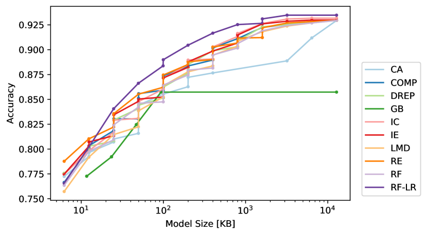
Figure 2: 5-fold cross-validation accuracy over the size of the ensemble on the EEG dataset. Single points are the individual parameter configurations whereas the solid line depicts the corresponding Pareto front. Best viewed in color.

Figure 3 shows the results on the chess dataset. Here the accuracy ranges from $28\%$ to $75\%$ with model sizes up to $12$ MB (again note the logarithmic scale on the x-axis). Similar to before, the pruning methods all converge against similar solutions just above $65\%$. CA still seems to perform poorly for smaller model sizes, but not as bad as on the EEG data. Similar, GB also seems to struggle on this dataset. It is worth noting, that some pruning methods (e.g. IC or RE) have a better accuracy-memory trade-off compared to Random Forest and they outperform the original forest by about $2\%$. RF-LR offers the best performance on this dataset and outperforms the original forest by about $8\%$ accuracy across all model sizes. This effect is only present for RF-LR and cannot be seen for the other methods. Overall, RF-LR offers a much better accuracy-memory trade-off and offers the best overall accuracy.

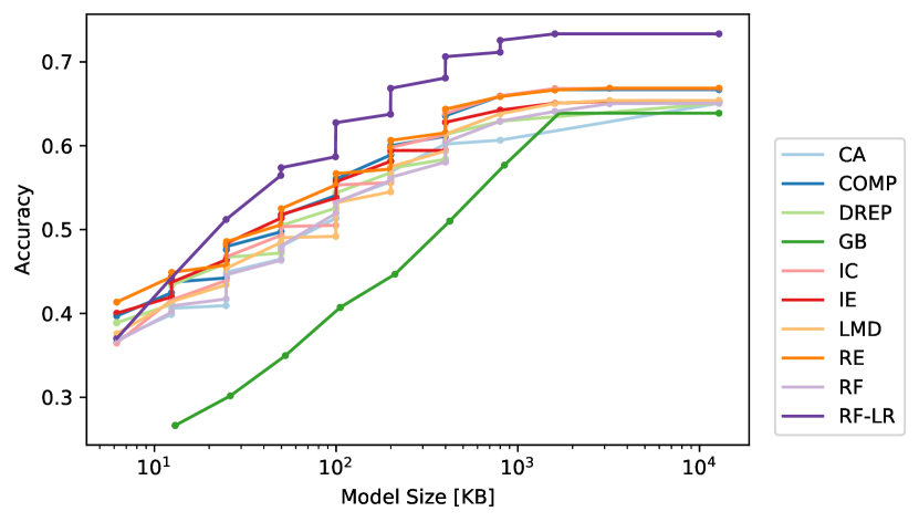
Figure 3: 5-fold cross-validation accuracy over the size of the ensemble on the chess dataset. Single points are the individual parameter configurations whereas the solid line depicts the corresponding Pareto front. Best viewed in color.

Conclusion: First we find that the well-performing RF models often require more than $1$ MB easily breaking the available memory on small MCUs (cf. Table 1). Second, we found two different behaviors of RF-LR: In many cases all methods converge against a similar accuracy when more memory is available, e.g. as seen in Figure 2. This can be expected since all methods derive their models from the same RF model. Here, RF-LR often has better models and hence offers a better accuracy-memory trade-off. In many other cases we found that RF-LR significantly outperforms the other methods and offers a much better accuracy across most model sizes, e.g. as depicted in Figure 3. In these cases, RF-LR offers a much better accuracy-memory trade-off and the best overall accuracy.

5.2 Quantitative Analysis

The previous section showed that RF-LR can offer substantial improvements on some datasets and smaller improvements in other cases. To give a more complete picture we will now look at the performance of each method under various memory constraints. Table 3 shows the best accuracy of each method (across all hyperparameter configurations) with a final model size below $64$ KB. Such models could for example easily be deployed on an Arduino Due MCU (cf. Table 1). We find that RF-LR offers the best accuracy in $9$ out of $16$ cases followed by RE which is first in $4$ cases followed by GB with ranks first in $3$ cases. IE shares the first place with RE on the mozilla dataset. On some datasets such as ida2016 the differences are comparably small which can be expected since all models are derived from the same base Random Forest. However, on other datasets such as the eeg, chess, japanese-vowels or connect dataset we can find more substantial improvements where RF-LR offers up to $5\%$ better accuracy to the second ranking method.

A similar picture can be find in Table 4 which shows the best accuracy of each method (across all hyperparameter configurations) with a final model size below $256$ KB. Such models could for example easily be deployed on an STM32F4 MCU (cf. Table 1). Now RF-LR offers the best accuracy in $10$ out of $16$ cases followed by RE which is first in only $1$ case followed by GB with ranks first in $2$ cases and IC which is now first in $3$ cases. IE now shares the first place with IC on the mozilla dataset. As before, the differences are comparably small on some datasets (e.g. the mozilla dataset) and more substantial on other datasets where RF-LR now offers up $6\%$ better accuracy against the second best method.

model	CA	COMP	DREP	GB	IC	IE	LMD	RE	RF	RF-LR
adult	85.455	85.777	85.618	86.616	85.799	85.882	85.378	86.128	85.464	86.241
anura	96.511	97.137	96.873	95.024	97.192	96.928	96.539	97.067	96.525	97.512
avila	91.930	96.957	95.318	67.724	96.760	96.689	86.965	97.048	92.534	94.278
bank	89.772	90.049	89.927	90.677	90.213	90.330	89.819	90.336	89.830	90.522
chess	48.025	51.714	50.492	34.969	50.356	51.793	49.041	52.495	48.090	57.382
connect	72.426	73.898	73.409	70.847	73.724	73.832	73.110	74.134	72.666	77.498
eeg	84.419	85.574	84.419	82.463	84.780	85.033	83.852	85.527	84.606	86.622
elec	83.523	83.620	84.075	83.878	82.749	84.556	82.817	84.680	83.391	84.894
ida2016	99.044	99.119	99.025	99.094	99.106	99.100	99.031	99.125	99.075	99.219
japanese-vowels	90.061	91.487	91.045	87.341	91.517	90.332	90.794	91.587	90.503	93.173
magic	86.109	86.613	86.282	87.355	86.692	86.771	86.456	86.845	86.419	86.997
mnist	80.700	85.700	84.300	74.400	84.700	84.100	85.000	84.900	84.200	87.000
mozilla	94.590	94.764	94.661	94.590	94.815	94.860	94.468	94.860	94.545	94.699
nomao	95.508	95.804	95.575	95.958	95.749	95.819	95.358	95.802	95.633	96.063
postures	79.913	81.688	80.827	69.058	81.137	80.996	79.599	81.727	80.246	81.081
satimage	88.647	88.880	88.663	87.449	88.911	88.616	88.647	89.020	88.538	88.834

Table 3: Test accuracies for models with a memory consumption below $64$ KB for each method and each dataset averaged over a $5$ fold cross validation. Rounded to the third decimal digit. Larger is better. The best method is depicted in bold. More details on the experiments and datasets can be find in the appendix.

model	CA	COMP	DREP	GB	IC	IE	LMD	RE	RF	RF-LR
adult	85.774	86.174	85.956	87.135	86.011	86.232	85.738	86.272	85.799	86.508
anura	96.511	97.818	97.748	97.429	98.040	97.929	97.582	97.818	97.735	98.013
avila	95.016	99.022	97.427	82.820	99.176	99.123	93.315	99.248	96.526	98.807
bank	89.967	90.297	90.082	90.737	90.290	90.443	89.952	90.471	90.038	90.874
chess	56.911	59.998	57.314	44.678	59.791	59.428	57.496	60.636	56.238	66.852
connect	74.522	76.270	75.119	76.170	76.239	76.333	75.100	76.303	74.997	80.340
eeg	87.223	88.364	88.511	85.734	88.959	88.778	87.784	88.785	87.951	90.454
elec	85.220	85.810	85.832	85.748	86.043	86.692	84.922	86.562	85.362	87.829
ida2016	99.106	99.225	99.119	99.169	99.262	99.175	99.238	99.175	99.194	99.244
japanese-vowels	91.979	94.810	94.428	94.860	94.790	94.077	94.278	94.709	94.408	96.205
magic	86.655	87.281	87.218	87.733	87.234	87.239	87.302	87.365	86.950	87.570
mnist	86.900	90.100	89.300	84.600	90.600	89.700	88.800	89.600	89.300	91.800
mozilla	94.731	95.034	94.982	94.989	95.092	95.092	94.802	94.995	94.912	95.014
nomao	96.039	96.222	96.150	96.408	96.318	96.269	96.077	96.356	96.135	96.539
postures	88.587	89.596	88.747	81.100	89.231	89.390	88.085	89.633	88.281	90.504
satimage	88.802	90.218	89.891	89.782	89.705	89.891	90.000	90.156	90.016	90.715

Table 4: Test accuracies for models with a memory consumption below $256$ KB for each method and each dataset averaged over a $5$ fold cross validation. Rounded to the third decimal digit. Larger is better. The best method is depicted in bold. More details on the experiments and datasets can be find in the appendix.

	CA	COMP	DREP	GB	IC	IE	LMD	RE	RF	RF-LR
chess	0.6251	0.6628	0.6363	0.6265	0.6638	0.6489	0.6486	0.6644	0.6441	0.7290
connect	0.7570	0.7712	0.7608	0.7780	0.7733	0.7726	0.7623	0.7737	0.7607	0.8219
eeg	0.9050	0.9242	0.9240	0.8570	0.9276	0.9258	0.9224	0.9242	0.9225	0.9319
elec	0.8667	0.8767	0.8722	0.8572	0.8787	0.8779	0.8714	0.8783	0.8720	0.8974
postures	0.9390	0.9497	0.9436	0.9105	0.9504	0.9486	0.9460	0.9501	0.9460	0.9688
anura	0.9710	0.9791	0.9790	0.9766	0.9795	0.9791	0.9780	0.9792	0.9779	0.9800
bank	0.9018	0.9050	0.9038	0.9073	0.9052	0.9050	0.9034	0.9052	0.9034	0.9083
japanese-vowels	0.9568	0.9721	0.9717	0.9734	0.9731	0.9712	0.9719	0.9722	0.9707	0.9741
magic	0.8748	0.8783	0.8786	0.8772	0.8793	0.8788	0.8788	0.8795	0.8783	0.8808
mnist	0.9295	0.9393	0.9399	0.9377	0.9415	0.9400	0.9393	0.9403	0.9366	0.9432
nomao	0.9647	0.9678	0.9676	0.9640	0.9681	0.9678	0.9679	0.9677	0.9678	0.9682
adult	0.8620	0.8638	0.8630	0.8712	0.8642	0.8640	0.8627	0.8639	0.8631	0.8656
avila	0.9715	0.9924	0.9897	0.9909	0.9965	0.9963	0.9750	0.9930	0.9886	0.9928
ida2016	0.9901	0.9916	0.9908	0.9915	0.9913	0.9909	0.9909	0.9908	0.9907	0.9912
mozilla	0.9493	0.9520	0.9520	0.9498	0.9522	0.9525	0.9513	0.9526	0.9519	0.9526
satimage	0.9059	0.9135	0.9133	0.9119	0.9147	0.9150	0.9140	0.9135	0.9138	0.9148

Table 5: Normalized area under the Pareto front (APF) for each method and each dataset averaged over a $5$ fold cross validation. Rounded to the fourth decimal digit. Larger is better. The best method is depicted in bold.

To give a more complete picture across different memory constraints we will now summarize the performance of each method by the (normalized) area-under the Pareto front: Intuitively, we want to have an algorithm which gives small and accurate models and therefore places itself in the upper-left corner of the accuracy-memory plots. Similar to ‘regular’ ROC-AUC curves we can compute the area under the Pareto front (APF) normalized by the biggest model to summarize the accuracy for different models on the same dataset. Table 5 depicts the normalized APF for the experiments. Looking at RF-LR, we see that it is the clear winner. In total, it is the best method on 11 of 14 datasets, shares the first place on 1 dataset (mozilla), is the second best method on 1 data-set (satimage), third best method (ida2016) and fourth best methond (avila) each on one dataset. In the first block of datasets (chess, connect, eeg, elec, postures) RF-LR achieves substantial improvements with $1\%-8\%$ higher accuracies on average. Looking at the second block (adult, anura, bank, magic, mnist, nomao, japanese-vowels) RF-LR is still the best method, but the differences are smaller than before. Finally, in block three (ida2016,mozilla,satimage) RF-LR is not the best method alone anymore, but ranks among the best methods.

Table 5 implies that RF-LR can offer substantial improvements in some cases and moderate improvement in many other cases. To give a statistical meaningful comparison we present the results in Table 5 as a CD diagram Demšar (2006). A CD diagram ranks each method according to its performance on each dataset. Then, a Friedman-Test is performed to determine if there is a statistical difference between the average rank of each method. If this is the case, a pairwise Wilcoxon-Test between all methods is used to check whether there is a statistical difference between two classifiers. CD diagrams visualize this evaluation by plotting the average rank of each method on the x-axis and connect all classifiers whose performances are statistically similar via a horizontal bar.

Figure 4 shows the CD diagram for the experiments, where $p=0.95$ was used for all statistical tests. RF-LR is the clear winner in this comparison. Its average rank is close to $1.5$ and it has some distance to the second best method IC with an average rank around $2.5$. It offers a statistically better performance compared to $\{RE,IE,COMP,LMD,DREP,RF,GB,CA\}$. The second clique is given by $\{IC,RE,IE,COMP,LMD,DREP,RF,GB\}$ with ranks around $2.5-7$. Overall, RE places third with an average rank around $4$ which shows that a simple method can perform surprisingly well. We hypothesize that since RE minimizes the overall ensemble loss that it finds a good balance between the bias and the diversity of the ensemble as e.g. discussed in Buschjäger et al. (2020). Next, $\{RF,GB,CA\}$ form the last clique with statistically similar performances which shows that a unpruned RF and GB doe not offer a good accuracy-memory trade-off. CA ranks last with some distance to the other methods. We are not sure why CA has such a bad performance and suspect a bug in our implementation which we could not find so far.

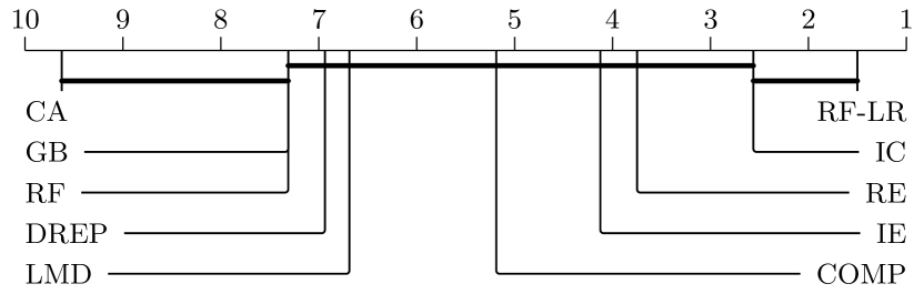
Figure 4: CD-Diagram for the normalized area under the Pareto front for different methods over multiple datasets. For all statistical tests $p=0.95$ was used. More to the right (lower rank) is better. Methods in connected cliques are statistically similar.

5.3 Case-Study On Raspberry Pi0

To showcase the effectiveness of our approach we will now compare the performance of ensemble pruning and leaf-refinement on a Raspberry Pi0. The Raspbery Pi0 has 512 MB RAM and uses a BCM 2835 SOC CPU clocked at 1 GHz. This makes it considerably more powerful than the MCUs mentioned in Table 1, but also allows us to run a full Linux environment which simplifies the evaluation. Again we will now focus on the EEG dataset as our standard example. From our previous experiment we selected pruning configurations that resulted in an ensemble size below $256$ KB and generate ensemble-specific C++ code as outline in Buschjäger et al. (2018) which is then compiled on the Pi0 itself. We compare the latency, the accuracy and the total binary size of these implementations. Note that the total binary size may exceed 256 KB because the binary also contains additional functions from the standard library as well as a start routine and the corresponding ELF header. However, this overhead is the same for all implementations. For simplicity we measure the accuracy as well as the latency using the first cross-validation set. To ensure a fair comparison we repeat each experiment 5 times. Table 6 contains the results for this evaluation. As one can see the binary sizes range from $268$ KB to roughly $800$ KB and each implementation requires $0.8$ to $1.6$ µs to classify a single observation. As expected, RF-LR offers the best accuracy around $91$ % while ranking third in memory usage. Somewhat surprisingly, RF-LR has a comparably high latency. We conjecture that the structure of the trees in RF-LR is not very homogeneous which seems to be beneficial for the accuracy, but may hurt the caching behavior of the trees. A more thorough discussion can be found in Buschjäger et al. (2018) on this topic and a combination of of both approaches should be considered in future research. Nevertheless, this evaluation shows that our approach can be applied in a real-world scenario and we believe that these results can be transferred to other hardware architectures as well.

Method	Accuracy	Size [Bytes]	Latency [µs/obs.]
CA	86.2817	268 536	0.80107
COMP	89.8531	689 712	1.06809
DREP	88.7850	342 696	1.00134
IC	89.2523	793 280	1.06809
IE	88.8518	743 232	1.00134
LMD	88.8518	784 896	1.06809
RE	89.2523	792 456	1.13485
RF	89.5194	588 336	1.60214
RF-LR	91.0881	588 088	1.46862

Table 6: Accuracy, Size and Latency on a Raspberry Pi0. Models are filtered so that the ensemble size does not exceed $256$ KB.

6 Conclusion

Ensemble algorithms are among the state-of-the-art in many machine learning applications. With the ongoing integration of ML models into everyday life, the deployment and continuous application of models becomes more and more an important issue. By today’s standard, Random Forests are trained with large trees for the best performance which can challenge the resources of small devices and sometimes make deployment impossible. Ensemble pruning is a standard technique to remove unnecessary classifiers from the ensemble to reduce the overall resource consumption while potentially improving its accuracy. This makes ensemble pruning ideal to bring accurate ensembles to small devices. While ensemble pruning improves the performance of ensembles of small trees we found that this improvement diminishes for ensembles of large trees. Moreover, it does not offer fine-grained control over this trade-off because it removes entire trees at once from the ensemble. We argue that, from a hardware perspective, the fine-grained control over the accuracy-memory trade-off is what really matters. We propose a simple and surprisingly effective algorithm which refines the predictions of the trees in a forest using SGD. We compared our Leaf-Refinement method against 7 state-of-the-art pruning methods on $16$ datasets. Leaf-Refinement outperforms the other methods on 11 of 16 datasets with a statistically significant better accuracy-memory trade-off compared to most methods. In a small study we showed that our approach can be applied in real-world scenarios. and we believe that our results can be transferred to other hardware architectures. Since our approach is orthogonal to existing approaches it can be freely combined with other methods for efficient deployment. Hence future research should include not only the combination of more diverse hardware, but also the combination of different methods.

References

- Barros et al. (2015) Barros, R. C., de Carvalho, A. C. P. L. F., and Freitas, A. A. Decision-Tree Induction, pp. 7–45. Springer International Publishing, Cham, 2015. ISBN 978-3-319-14231-9. doi: 10.1007/978-3-319-14231-9˙2. URL https://doi.org/10.1007/978-3-319-14231-9_2.
- Biau (2012) Biau, G. Analysis of a random forests model. Journal of Machine Learning Research, 13(Apr):1063–1095, 2012.
- Biau & Scornet (2016) Biau, G. and Scornet, E. A random forest guided tour. Test, 25(2):197–227, 2016.
- Branco et al. (2019) Branco, S., Ferreira, A. G., and Cabral, J. Machine learning in resource-scarce embedded systems, fpgas, and end-devices: A survey. Electronics, 8(11):1289, 2019.
- Breiman (1996) Breiman, L. Bagging predictors. Machine learning, 24(2):123–140, 1996.
- Breiman (2000) Breiman, L. Some infinity theory for predictor ensembles. Technical report, Technical Report 579, Statistics Dept. UCB, 2000.
- Buschjäger & Morik (2017) Buschjäger, S. and Morik, K. Decision tree and random forest implementations for fast filtering of sensor data. IEEE Transactions on Circuits and Systems I: Regular Papers, 65(1):209–222, 2017.
- Buschjäger et al. (2020) Buschjäger, S., Pfahler, L., and Morik, K. Generalized negative correlation learning for deep ensembling. arXiv preprint arXiv:2011.02952, 2020.
- Buschjäger et al. (2018) Buschjäger, S., Chen, K., Chen, J., and Morik, K. Realization of random forest for real-time evaluation through tree framing. In ICDM, pp. 19–28, 2018. doi: 10.1109/ICDM.2018.00017.
- Cavalcanti et al. (2016) Cavalcanti, G. D., Oliveira, L. S., Moura, T. J., and Carvalho, G. V. Combining diversity measures for ensemble pruning. Pattern Recognition Letters, 74:38–45, 2016.
- Choudhary et al. (2020) Choudhary, T., Mishra, V., Goswami, A., and Sarangapani, J. A comprehensive survey on model compression and acceleration. Artificial Intelligence Review, 53(7):5113–5155, 2020.
- Cortes et al. (2014) Cortes, C., Mohri, M., and Syed, U. Deep boosting. In Proceedings of the Thirty-First International Conference on Machine Learning (ICML 2014), 2014.
- Demšar (2006) Demšar, J. Statistical comparisons of classifiers over multiple data sets. The Journal of Machine Learning Research, 7:1–30, 2006.
- Denil et al. (2014) Denil, M., Matheson, D., and De Freitas, N. Narrowing the gap: Random forests in theory and in practice. In International conference on machine learning (ICML), 2014.
- Domingos (2000) Domingos, P. A unified bias-variance decomposition for zero-one and squared loss. AAAI/IAAI, 2000:564–569, 2000.
- Friedman (2001) Friedman, J. H. Greedy function approximation: a gradient boosting machine. Annals of statistics, pp. 1189–1232, 2001.
- Geurts et al. (2006) Geurts, P., Ernst, D., and Wehenkel, L. Extremely randomized trees. Machine learning, 63(1):3–42, 2006.
- Giacinto et al. (2000) Giacinto, G., Roli, F., and Fumera, G. Design of effective multiple classifier systems by clustering of classifiers. In Proceedings 15th International Conference on Pattern Recognition. ICPR-2000, volume 2, pp. 160–163. IEEE, 2000.
- Guo et al. (2018) Guo, H., Liu, H., Li, R., Wu, C., Guo, Y., and Xu, M. Margin & diversity based ordering ensemble pruning. Neurocomputing, 275:237–246, 2018.
- Ho (1998) Ho, T. K. The random subspace method for constructing decision forests. IEEE transactions on pattern analysis and machine intelligence, 20(8):832–844, 1998.
- Jiang et al. (2017) Jiang, Z., Liu, H., Fu, B., and Wu, Z. Generalized ambiguity decompositions for classification with applications in active learning and unsupervised ensemble pruning. 31st AAAI Conference on Artificial Intelligence, AAAI 2017, pp. 2073–2079, 2017.
- Koltchinskii et al. (2002) Koltchinskii, V. et al. Empirical margin distributions and bounding the generalization error of combined classifiers. The Annals of Statistics, 30(1):1–50, 2002.
- Kumar et al. (2017) Kumar, A., Goyal, S., and Varma, M. Resource-efficient machine learning in 2 kb ram for the internet of things. In International Conference on Machine Learning, pp. 1935–1944. PMLR, 2017.
- Lazarevic & Obradovic (2001) Lazarevic, A. and Obradovic, Z. Effective pruning of neural network classifier ensembles. In IJCNN’01, volume 2, pp. 796–801. IEEE, 2001.
- Li et al. (2012) Li, N., Yu, Y., and Zhou, Z.-H. Diversity regularized ensemble pruning. In ECML PKDD, pp. 330–345. Springer, 2012.
- Louppe & Geurts (2012) Louppe, G. and Geurts, P. Ensembles on random patches. In Joint European Conference on Machine Learning and Knowledge Discovery in Databases, pp. 346–361. Springer, 2012.
- Lu et al. (2010) Lu, Z., Wu, X., Zhu, X., and Bongard, J. Ensemble pruning via individual contribution ordering. In Proc. of the ACM SIGKDD, pp. 871–880, 2010.
- Margineantu & Dietterich (1997) Margineantu, D. D. and Dietterich, T. G. Pruning adaptive boosting. In ICML, volume 97, pp. 211–218, 1997.
- Martınez-Munoz & Suárez (2004) Martınez-Munoz, G. and Suárez, A. Aggregation ordering in bagging. In Proc. of the IASTED, pp. 258–263, 2004.
- Martínez-Muñoz & Suárez (2006) Martínez-Muñoz, G. and Suárez, A. Pruning in ordered bagging ensembles. In ICML, pp. 609–616, 2006.
- Martínez-Muñoz et al. (2008) Martínez-Muñoz, G., Hernández-Lobato, D., and Suárez, A. An analysis of ensemble pruning techniques based on ordered aggregation. IEEE Transactions on Pattern Analysis and Machine Intelligence, 31(2):245–259, 2008.
- Oshiro et al. (2012) Oshiro, T. M., Perez, P. S., and Baranauskas, J. A. How many trees in a random forest? In International workshop on machine learning and data mining in pattern recognition, pp. 154–168. Springer, 2012.
- Pedregosa et al. (2011) Pedregosa, F., Varoquaux, G., Gramfort, A., Michel, V., Thirion, B., Grisel, O., Blondel, M., Prettenhofer, P., Weiss, R., Dubourg, V., Vanderplas, J., Passos, A., Cournapeau, D., Brucher, M., Perrot, M., and Duchesnay, E. Scikit-learn: Machine learning in Python. Journal of Machine Learning Research, 12:2825–2830, 2011.
- Shotton et al. (2013) Shotton, J., Sharp, T., Kohli, P., Nowozin, S., Winn, J., and Criminisi, A. Decision jungles: Compact and rich models for classification. In NIPS’13 Proceedings of the 26th International Conference on Neural Information Processing Systems, pp. 234–242, 2013.
- Tsoumakas et al. (2009) Tsoumakas, G., Partalas, I., and Vlahavas, I. An ensemble pruning primer. In Applications of supervised and unsupervised ensemble methods. Springer, 2009.
- Ye et al. (2018) Ye, T., Zhou, H., Zou, W. Y., Gao, B., and Zhang, R. Rapidscorer: fast tree ensemble evaluation by maximizing compactness in data level parallelization. In Proceedings of the 24th ACM SIGKDD International Conference on Knowledge Discovery & Data Mining, pp. 941–950, 2018.
- Zhang et al. (2006) Zhang, Y., Burer, S., and Street, W. N. Ensemble pruning via semi-definite programming. Journal of machine learning research, 7(Jul):1315–1338, 2006.
- Zhou (2012) Zhou, Z.-H. Ensemble methods: foundations and algorithms. CRC press, 2012.
- Zhou et al. (2002) Zhou, Z.-H., Wu, J., and Tang, W. Ensembling neural networks: many could be better than all. Artificial intelligence, 137(1-2):239–263, 2002.