Extraction of $B_{s}\to D^{(*)}_{s}$ form factors from ${N_{f}}=2$ lattice QCD

Abstract

We report on a two-flavour lattice QCD study of the $B_{s}\to D_{s}$ and $B_{s}\to D^{*}_{s}$ transitions parameterized, in the heavy quark limit, by the form factors ${\cal G}$, and $h_{A_{1}}$, $h_{A_{2}}$ and $h_{A_{3}}$, respectively. In the search for New Physics through tests of lepton flavour universality, $B_{s}$ decay channels are complementary to the $B$ decays widely studied at $B$ factories and LHCb, while on the theory side they can be better controlled than the $B_{c}$ and $\Lambda_{b}$ decays. The purpose of this exploratory two-flavour study is, in preparation for future analyses of lattice QCD simulations with ${N_{f}>2}$ and physical quark-masses, to gain experience on a suitable method for a lattice extraction of form factors associated with $b\to c$ currents that may yield tighter control over systematic effects like contamination from excited states and cut-off effects. We obtain the zero-recoil values ${\cal G}^{B_{s}\to D_{s}}(1)=1.03(14)$ and $h^{B_{s}\to D^{*}_{s}}(1)=0.85(16)$.

1 Introduction

Though the Standard Model of particle physics (SM) has shown to describe the fundamental interactions up to the electroweak scale pretty well, experimental measurements sometimes give results that were totally unexpected. In particular, a recent and spectacular example in flavour physics phenomenology is the so-called $B$ anomalies in the test of lepton flavour universality in $b\to c$ semileptonic decays. The ratio of decay widths $R_{H_{c}}\equiv\frac{\Gamma(H_{b}\to H_{c}\tau\nu_{\tau})}{\Gamma(H_{b}\to H_{c}\ell\nu_{\ell})_{\ell=e,\mu}}$ has been considered in cases $(H_{b},H_{c})=(B,D)$, $(B,D^{*})$ and $(B_{c},J/\psi)$ and compared with theoretical expectations. A discrepancy of $2\sigma$ has been observed for $R_{D}$ [1, 2, 3, 4, 5, 6, 7, 8, 9, 10], $3\sigma$ for $R_{D^{*}}$ [11, 12, 13, 14, 8, 9, 15, 10] and $\sim\sigma$ for $R_{J/\psi}$ [16, 17]. A bunch of New Physics models have been advocated to explain those discrepancies, together with other anomalies in $b\to s\ell\ell$ transitions, like models with extra doublets of Higgs fields [18] or with leptoquarks [19]. Further measurements are led to explore more $b\to c$ processes, such as $\Lambda_{b}\to\Lambda_{c}l\nu_{l}$ or $B_{s}\to D^{(*)}_{s}l\nu$, and are expected to come soon at LHCb and Belle 2.

A theoretical effort has been undertaken to extract the form factors associated with $B_{s}\to D^{(*)}_{s}l\nu$, but the number of results is still limited [20, 21, 22, 23, 24, 25]. Our aim here is to study whether Wilson-Clover fermions, in combination with the step-scaling in mass method [26, 20], provide a suitable lattice regularisation to get reliable results for these processes, as far as cut-off effects and contamination by excited states are concerned. While our current exploratory work focuses on $N_{f}=2$, any phenomenologically relevant application of the methods investigated here has to be done in lattice QCD with $N_{f}=2+1(+1)$ flavours.

The paper is organised as follows: in Section 2 we highlight the strategy we have come up with, in Section 3 we give the simulation details and collect our raw data. In Section 4 we present our analysis and comment on the results. Section 5 contains the conclusion.

2 Strategy

The starting point is to consider the hadronic matrix element $\langle D_{s}(p_{D_{s}})|V^{\mu}|H_{s}(p_{H_{s}})\rangle$, with $V^{\mu}=\bar{c}\gamma^{\mu}h$. Its Lorentz structure decomposition reads

$$\langle D_{s}(p_{D_{s}})|V^{\mu}|H_{s}(p_{H_{s}})\rangle=f^{+}(q^{2})(p_{D_{s}}+p_{H_{s}})^{\mu}+f^{-}(q^{2})q^{\mu},$$ (2.1)

with the quantities $f^{+}$ and $f^{-}$ familiar as form factors depending on $q=p_{H_{s}}-p_{D_{s}}$. We will be interested in the physics case $H_{s}\equiv B_{s}$. In phenomenology it is convenient to introduce the scalar form factor $f_{0}$ defined by:

$$\langle D_{s}(p_{D_{s}})|V^{\mu}|H_{s}(p_{H_{s}})\rangle=f^{+}(q^{2})\left[(p_{D_{s}}+p_{H_{s}})^{\mu}-\frac{m^{2}_{H_{s}}-m^{2}_{D_{s}}}{q^{2}}q^{\mu}\right]+f_{0}(q^{2})\frac{m^{2}_{H_{s}}-m^{2}_{D_{s}}}{q^{2}}q^{\mu},$$ (2.2)

Hence, we have

$$f^{-}(q^{2}) = \frac{m^{2}_{H_{s}}-m^{2}_{D_{s}}}{q^{2}}[f_{0}(q^{2})-f^{+}(q^{2})],$$ (2.3)

$$f_{0}(q^{2}) = f^{+}(q^{2})+f^{-}(q^{2})\frac{q^{2}}{m^{2}_{H_{s}}-m^{2}_{D_{s}}}.$$ (2.4)

With the kinematical configuration of an $H_{s}$-meson at rest, we can write

$$\langle D_{s}(p_{D_{s}})|V^{0}|H_{s}(p_{H_{s}})\rangle = f^{+}(q^{2})(E_{D_{s}}+m_{H_{s}})+f^{-}(q^{2})(m_{H_{s}}-E_{D_{s}}),$$

$$\langle D_{s}(p_{D_{s}})|V^{i}|H_{s}(p_{H_{s}})\rangle = -q^{i}(f^{+}(q^{2})-f^{-}(q^{2})).$$ (2.5)

When the $H_{s}$ meson is put at rest, the recoil $w=\frac{p_{D_{s}}\cdot p_{H_{s}}}{m_{H_{s}}m_{D_{s}}}\equiv v_{H_{s}}\cdot v_{D_{s}}$ has the simple expression $w=E_{D_{s}}/m_{D_{s}}$. Our goal is to extract the form factor $f^{+}(B_{s}\to D_{s})$ at zero recoil, $w=1$. However, except in the elastic case $D_{s}\to D_{s}$ where one finds trivially that $f^{+}(w=1)=1$, this kinematical point is not directly accessible to a lattice measurement. It is only by extrapolating in $w$ that one can obtain results at zero recoil. With $\vec{q}=-(\theta,\theta,\theta)$, $w\sim\sqrt{m_{D_{s}}^{2}+3\theta^{2}}/m_{D_{s}}$, we have

$$f^{+}(w) = \frac{1}{2m_{H_{s}}}\left[\langle D_{s}(p_{D_{s}})|V^{0}|H_{s}(p_{H_{s}})\rangle+\frac{m_{H_{s}}-E_{D_{s}}}{3\theta}\sum_{i}\langle D_{s}(p_{D_{s}})|V^{i}|H_{s}(p_{H_{s}})\rangle\right],$$

$$f^{-}(w) = \frac{1}{2m_{H_{s}}}\left[\langle D_{s}(p_{D_{s}})|V^{0}|H_{s}(p_{H_{s}})\rangle-\frac{m_{H_{s}}+E_{D_{s}}}{3\theta}\sum_{i}\langle D_{s}(p_{D_{s}})|V^{i}|H_{s}(p_{H_{s}})\rangle\right].$$

On the other hand, in the framework of Heavy Quark Effective Theory (HQET), it is also common to parameterise the matrix element in question in terms of the form factors $h^{\pm}(w)$,

$$\frac{\langle D_{s}(p_{D_{s}})|V^{\mu}|H_{s}(p_{H_{s}})\rangle}{\sqrt{m_{D_{s}}m_{H_{s}}}}=h^{+}(w)(v_{D_{s}}+v_{H_{s}})^{\mu}+h^{-}(w)(v_{H_{s}}-v_{D_{s}})^{\mu},$$ (2.7)

$$h^{+}(w) = \frac{1}{2\sqrt{m_{D_{s}}m_{H_{s}}}}\left[(m_{H_{s}}+m_{D_{s}})f^{+}(w)+(m_{H_{s}}-m_{D_{s}})f^{-}(w)\right],$$

$$h^{-}(w) = \frac{1}{2\sqrt{m_{D_{s}}m_{H_{s}}}}\left[(m_{H_{s}}-m_{D_{s}})f^{+}(w)+(m_{H_{s}}+m_{D_{s}})f^{-}(w)\right],$$ (2.8)

with the aid of which one introduces the factors ${\cal G}(w)$ and $H(w)$:

$${\cal G}(w) = h^{+}(w)\left[1-\frac{m_{H_{s}}-m_{D_{s}}}{m_{H_{s}}+m_{D_{s}}}\frac{h^{-}(w)}{h^{+}(w)}\right]$$ (2.9)

$$= h^{+}(w)\left[1-\left(\frac{m_{H_{s}}-m_{D_{s}}}{m_{H_{s}}+m_{D_{s}}}\right)^{2}H(w)\right],$$

$$H(w) = \frac{m_{H_{s}}+m_{D_{s}}}{m_{H_{s}}-m_{D_{s}}}\frac{h^{-}(w)}{h^{+}(w)}.$$ (2.10)

$h^{\pm}(1)$, $f^{\pm}(1)$ and $f_{0}(1)$ can then be extracted by doing a polynomial extrapolation in $w-1$. In the following we will concentrate on estimating of ${\cal G}^{B_{s}\to D_{s}}(w=1)$.

To obtain results at the $b$ quark mass (while trying to keep cut-off effects under control) we have decided to apply the strategy of step-scaling in masses [26, 20] that was already adapted to the Wilson-Clover regularisation in [27]. Steps in RGI heavy quark mass cannot be used at this stage of knowledge as far as the Wilon-Clover regularisation is concerned. Indeed without a still unknown $O(a^{2})$ term in an improvement factor, the RGI quark mass becomes negative, hence unphysical, for quark masses greater than $\sim 2m_{c}$ and the lattice spacings at our disposal.

The idea is to consider ratios of ${\cal G}(1)$ at 2 consecutive heavy-strange meson masses $m_{H_{s}(i+1)}$ and $m_{H_{s}(i)}$ in the step-scaling mass chain:

$$\sigma^{i}_{\cal G}=\frac{{\cal G}(1,m_{H_{s}(i+1)})}{{\cal G}(1,m_{H_{s}(i)})},\quad m_{H_{s}(i)}=\lambda^{i}m_{D_{s}},\quad\lambda=\left(\frac{m_{B_{s}}}{m_{D_{s}}}\right)^{1/K},$$ (2.11)

where $K$ is the number of steps. Thus we have

$${\cal G}(1,m_{B_{s}})={\cal G}(1,m_{D_{s}})\times\prod_{i=0}^{K-1}\sigma^{i}_{\cal G},$$ (2.12)

with

$${\cal G}(1,m_{D_{s}}) = \lim_{a\to 0\,,\,m_{\pi}\to m^{\rm phys}_{\pi}}{\cal G}^{\rm lat}(1,m_{D_{s}},a,m_{\pi}),$$ (2.13)

$$\sigma^{i}_{\cal G} = \lim_{a\to 0\,,\,m_{\pi}\to m^{\rm phys}_{\pi}}\Sigma^{i}_{\cal G}(a,m_{\pi}),$$ (2.14)

where $\Sigma_{\mathcal{G}}^{i}=\frac{{\cal G}^{\rm lat}(m_{H_{s}(i)})}{{\cal G}^{\rm lat}(m_{H_{s}(i-1)})}$ is the ratio of successive $\cal{G}$’s on the given ensemble. By construction, ${\cal G}(1,m_{D_{s}})$ is equal to 1. It will be a useful check that our numerical data obey that constraint. Taking this into account, we have ${\cal G}(1,m_{B_{s}})=\prod_{i=0}^{K-1}\sigma^{i}_{\cal G}$.

Concerning the decay $H_{s}\to D^{*}_{s}$, a convenient framework is again HQET. Taking into account parities under $C$, $P$ and $T$ symmetries, the Lorentz structure decomposition of the hadronic matrix element $\langle D^{*}_{s}(p_{D^{*}_{s}},\epsilon^{(\lambda)})|A^{\mu}|H_{s}(p_{H_{s}})\rangle$ reads

$$\frac{\langle D^{*}_{s}(p_{D^{*}_{s}},\epsilon^{(\lambda)})|A^{\mu}|H_{s}(p_{H_{s}})\rangle}{2\sqrt{m_{H_{s}}m_{D^{*}_{s}}}}=\frac{i}{2}\epsilon^{*(\lambda)}_{\nu}[g^{\mu\nu}(1+w)h_{A_{1}}-v^{\mu}_{H_{s}}(v^{\nu}_{B_{s}}h_{A_{2}}+v^{\nu}_{D^{*}_{s}}h_{A_{3}})].$$ (2.15)

With

$$R^{\mu\rho}=\sum_{\lambda}\epsilon^{\rho(\lambda)}\langle D^{*}_{s}(p_{D^{*}_{s}},\epsilon^{(\lambda)})|A^{\mu}|H_{s}(p_{H_{s}})\rangle$$ (2.16)

and the normalisation equation of the polarisation vectors of a vector meson of mass $m_{V}$ and momentum $k$,

$$\sum_{\lambda}\epsilon^{\mu(\lambda)}\epsilon^{*\nu(\lambda)}=-g^{\mu\nu}+\frac{k^{\mu}k^{\nu}}{m^{2}_{V}},$$ (2.17)

we get

$$\frac{-R^{\mu\rho}}{2\sqrt{m_{H_{s}}m_{D^{*}_{s}}}} = \frac{i}{2}\left[\left(g^{\mu\rho}-\frac{p^{\mu}_{D^{*}_{s}}p^{\rho}_{D^{*}_{s}}}{m^{2}_{D^{*}_{s}}}\right)(1+w)h_{A_{1}}\right.$$ (2.18)

$$\left.\hskip 11.38092pt-\left(g^{\rho\nu}-\frac{p^{\rho}_{D^{*}_{s}}p^{\nu}_{D^{*}_{s}}}{m^{2}_{D^{*}_{s}}}\right)\left(v_{\nu\,B_{s}}v^{\mu}_{H_{s}}h_{A_{2}}+v_{\nu\,B_{s}}v^{\mu}_{D^{*}_{s}}h_{A_{3}}\right)\right].$$

Taking the $H_{s}$ meson at rest and $i,j$ as spatial indices, we obtain

$$\frac{-R^{ij}}{2\sqrt{m_{H_{s}}m_{D^{*}_{s}}}}=\frac{i}{2}\left[\left(g^{ij}-\frac{p^{i}_{D^{*}_{s}}p^{j}_{D^{*}_{s}}}{m^{2}_{D^{*}_{s}}}\right)(1+w)h_{A_{1}}+\frac{E_{D^{*}_{s}}p^{i}_{D^{*}_{s}}p^{j}_{D^{*}_{s}}}{m^{3}_{D^{*}_{s}}}h_{A_{3}}\right].$$ (2.19)

It means that we can determine two form factors, $h_{A_{1}}$ and $h_{A_{3}}$. With

$$A = \frac{1}{2\sqrt{m_{H_{s}}m_{D^{*}_{s}}}}\frac{i}{3}\sum_{i}R^{ii},$$

$$B = \frac{1}{2\sqrt{m_{H_{s}}m_{D^{*}_{s}}}}\frac{i}{6}\sum_{i\neq j}R^{ij}$$ (2.20)

and an isotropic momentum $\vec{p}_{D^{*}_{s}}=(\theta,\theta,\theta)$, we have

$$A = \frac{1}{2}\left[\left(1+\frac{\theta^{2}}{m^{2}_{D^{*}_{s}}}\right)(1+w)h_{A_{1}}-\frac{E_{D^{*}_{s}}\theta^{2}}{m^{3}_{D^{*}_{s}}}h_{A_{3}}\right],$$

$$B = \frac{1}{2}\left(\frac{\theta^{2}}{m^{2}_{D^{*}_{s}}}(1+w)h_{A_{1}}-\frac{E_{D^{*}_{s}}\theta^{2}}{m^{3}_{D^{*}_{s}}}h_{A_{3}}\right).$$ (2.21)

Thus, we arrive at

$$h_{A_{1}} = \frac{2}{w+1}(A-B),$$ (2.22)

$$h_{A_{3}} = \frac{m^{3}_{D^{*}_{s}}}{E_{D^{*}_{s}}\theta^{2}}\left[(w+1)\frac{\theta^{2}}{m^{2}_{D^{*}_{s}}}h_{A_{1}}-2B\right].$$ (2.23)

According to our step-scaling procedure, these quantities can finally be expressed as:

$$h_{A_{1}}(1,m_{B_{s}})=h_{A_{1}}(1,m_{D_{s}})\times\prod_{i=0}^{K-1}\sigma^{i}_{h_{A_{1}}}$$ (2.24)

$$R_{X_{3}}(1,m_{B_{s}}) \equiv \frac{h_{A_{3}}(1,m_{B_{s}})}{h_{A_{1}}(1,m_{B_{s}})}$$ (2.25)

$$= R_{X_{3}}(1,m_{D_{s}})\times\prod_{i=0}^{K-1}\sigma^{i}_{R_{X_{3}}},$$

with

$$h_{A_{1}}(1,m_{D_{s}}) = \lim_{a\to 0\,,\,m_{\pi}\to m^{\rm phys}_{\pi}}h_{A_{1}}^{\rm lat}(1,m_{D_{s}},a,m_{\pi}),$$ (2.26)

$$\sigma^{i}_{Y} = \lim_{a\to 0\,,\,m_{\pi}\to m^{\rm phys}_{\pi}}\Sigma^{i}_{Y}(a,m_{\pi}),\;\;Y=h_{A_{1}},R_{X_{3}}.$$ (2.27)

3 Computational setup

id	$\beta$	$(\frac{L}{a})^{3}\times\frac{T}{a}$	$\kappa_{\rm sea}$	$a~{}(\rm fm)$	$\frac{m_{\pi}}{\rm MeV}$	$Lm_{\pi}$	$\#$cfgs	$\kappa_{s}$	$\kappa_{c}$
A5	5.2	$32^{3}\times 64$	$0.13594$	0.0751	$333$	4.1	$198$	$0.135267$	$0.12531$
B6*		$48^{3}\times 96$	$0.13597$		$282$	5.2	$118$	$0.135257$	$0.12529$
E5	5.3	$32^{3}\times 64$	$0.13625$	0.0653	$439$	4.7	$200$	$0.135777$	$0.12724$
F6		$48^{3}\times 96$	$0.13635$		$313$	5	$120$	$0.135741$	$0.12713$
F7		$48^{3}\times 96$	$0.13638$		$268$	4.3	$200$	$0.135730$	$0.12713$
G8*		$64^{3}\times 128$	$0.13642$		$194$	4.1	$100$	$0.135705$	$0.12710$
N6	$5.5$	$48^{3}\times 96$	$0.13667$	$0.0483$	$341$	4	$192$	$0.136250$	$0.13026$
O7		$64^{3}\times 128$	$0.13671$		$269$	4.2	$60$	$0.136243$	$0.13022$

Table 1: Parameters of the simulations: bare coupling $\beta=6/g_{0}^{2}$, lattice resolution, hopping parameters of strange- and charm-quark masses, lattice spacing $a$ in physical units, pion mass, number of gauge configurations, bare strange and charm quark masses. (Ensembles with * were excluded from the extraction of $h_{A_{1}}$).

We have used in our analysis gauge field configuration ensembles generated by the CLS effort with $N_{f}=2$ non-perturbatively $\mathrm{O}(a)$ improved Wilson-Clover fermions [28, 29] and the plaquette gauge action [30]. The parameter $\kappa_{s}$ was taken from [31] and $\kappa_{c}$ from [32]. They have been used in previous works eg. [33, 27].

We have injected momenta to quarks by imposing isotropic twisted-boundary conditions in space, i.e. $\psi(x+L\vec{e}_{i})=e^{i\theta_{i}}\psi(x)$ with twisting angles $\theta_{i}$, $i=1,2,3$. The kinematics for 2-pt. and 3-pt. correlation function is depicted in Figure 1, where strange, charm and heavy flavours are denoted by $s$, $c$ and $h$, respectively. Only the charm quark carries the non-zero momentum. To reduce some of the ${O}(a^{2})$ effects we have averaged our results over positive and negative momenta. Six pairs $\pm\vec{\theta}$, in addition to the zero-momentum point, help us to extrapolate the various form factors associated with $H_{s}\to D_{s}$ and $H_{s}\to D^{*}_{s}$ from data available in the recoil region $1\leq w\lesssim 1.1$.

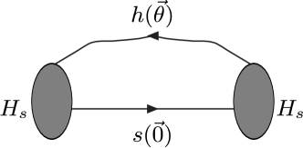
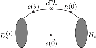
Figure 1: Kinematical configuration of the 2-pt. and 3-pt. correlation functions under study to extract the $H_{s}\to D^{(*)}_{s}$ form factors: the strange quark is always set at rest, while the $h\to c$ current inherits its momentum from the charm quark boundary condition. $\Gamma$ specifies the Dirac structure in question.

In Table 1 we collect the parameter specifications of the ensembles. Three lattice spacings $a_{\beta=5.5}=0.04831(38)$ fm, $a_{\beta=5.3}=0.06531(60)$ fm, $a_{\beta=5.2}=0.07513(79)$ fm, where the scale setting was performed in [34] via a fit in the chiral sector, are considered with pion masses in the range $[190\,\rm MeV\,,440\,\rm MeV]$. Heavy bare quark masses are the same as in [27]. Statistical errors have been computed employing the “$\Gamma$-method” [35], based on estimating autocorrelation functions. As in [27] all-to-all propagators were estimated stochastically with $U(1)$ spin-diluted walltime noise sources. We have also reduced the contamination by excited states on 2-pt. and 3-pt. correlators by solving a $4\times 4$ Generalized Eigenvalue Problem (GEVP) with one local and 3 Gaussian smeared interpolating fields. In the mass step-scaling strategy outlined above, we set $K=6$. In Table 2 we collect the twisting angles used to inject momenta to the charm quark. The phase shift was applied isotropically in all spatial directions.

id	$\theta\,[\pi/L]$
A5	{0.000, $\pm$ 0.150, $\pm$ 0.300, $\pm$ 0.525, $\pm$ 0.750, $\pm$ 1.050, $\pm$ 1.275}
B6	{0.000, $\pm$ 0.163, $\pm$ 0.326, $\pm$ 0.571, $\pm$ 0.815, $\pm$ 1.141, $\pm$ 1.385}
E5	{0.000, $\pm$ 0.125, $\pm$ 0.250, $\pm$ 0.438, $\pm$ 0.625, $\pm$ 0.875, $\pm$ 1.062}
F6	{0.000, $\pm$ 0.188, $\pm$ 0.375, $\pm$ 0.656, $\pm$ 0.938, $\pm$ 1.312, $\pm$ 1.594}
F7	{0.000, $\pm$ 0.188, $\pm$ 0.375, $\pm$ 0.656, $\pm$ 0.938, $\pm$ 1.312, $\pm$ 1.594}
G8	{0.000, $\pm$ 0.250, $\pm$ 0.500, $\pm$ 0.875, $\pm$ 1.250, $\pm$ 1.750, $\pm$ 2.125}
N6	{0.000, $\pm$ 0.254, $\pm$ 0.507, $\pm$ 0.887, $\pm$ 1.262, $\pm$ 1.774, $\pm$ 2.155}
O7	{0.000, $\pm$ 0.338, $\pm$ 0.676, $\pm$ 1.183, $\pm$ 1.683, $\pm$ 2.365, $\pm$ 2.873}

Table 2: Twisted angles of the charm quark field boundary condition that we use to inject momenta at the $h\to c$ current.

Our analysis involves the following 2-pt. correlation functions evaluated on the gauge field ensembles at hand:

$$C^{\theta,D_{s}}_{ij}(t) = \sum_{\vec{x}}\langle P^{\theta}_{cs,\,i}(t)P^{{\dagger}\,\theta}_{cs,\,j}(0)\rangle,$$

$$C^{H_{s}}_{ij}(t) = \sum_{\vec{x}}\langle P_{hs,\,i}(t)P^{{\dagger}}_{hs,\,j}(0)\rangle,$$

$$C^{\theta,D^{*}_{s}}_{ij}(t) = \frac{1}{3}\sum_{k=1}^{3}\sum_{\vec{x}}\langle V^{\theta}_{cs,\,k,\,i}(t)V^{{\dagger}\,\,\theta}_{cs,\,k,\,j}(0)\rangle,$$ (3.28)

where quark labels are as above, $i$ and $j$ specify smearing labels and spatial coordinates (summed over) are suppressed. The entering quark bilinears are defined as: $P_{hs}=\bar{\psi}_{h}\gamma^{5}\psi_{s}$, $P^{\theta}_{cs}=\bar{\psi}^{\theta}_{c}\gamma^{5}\psi_{s}$ and $V^{\theta}_{cs,\,k}=\bar{\psi}^{\theta}_{c}\gamma_{k}\psi_{s}$.

Now we continue with the 3-pt. correlation functions:

$$C^{\theta,PV^{I}_{\mu}P}_{ij}(t_{i},t) = \sum_{\vec{x},\vec{y}}\langle P_{hs,\,i}(t_{i})V^{I,\,\theta}_{hc,\,\mu}(t)P^{{\dagger}\,\theta}_{cs,\,j}(0)\rangle,$$

$$C^{\theta,PA^{I}_{k}V_{l}}_{ij}(t_{i},t) = \sum_{\vec{x},\vec{y}}\langle P_{hs,\,i}(t_{i})A^{I,\,\theta}_{hc,\,\mu}(t)V^{{\dagger}\,\theta}_{cs,l,\,j}(0)\rangle,$$ (3.29)

where the improved currents read $V^{I,\,\theta}_{hc,\,\mu}=\bar{\psi}_{h}\gamma_{\mu}\psi^{\theta}_{c}+ac_{V}\tilde{\partial}_{\nu}(\bar{\psi}_{h}\sigma_{\mu\nu}\psi^{\theta}_{c})$, and $A^{I,\,\theta}_{hc}=\bar{\psi}^{\theta}_{c}\gamma_{k}\gamma^{5}\psi_{h}+ac_{A}\tilde{\partial}_{k}(\bar{\psi}^{\theta}_{c}\gamma^{5}\psi_{h})$ with $\tilde{\partial}_{\mu}f(x)\equiv\frac{1}{2}({f(x+a\hat{\mu})-f(x-a\hat{\mu})})$.

Accordingly, we have to solve the three GEVPs

$$C^{\theta,D_{s}}_{ij}(t)v^{\theta,D_{s}}_{j}(t,t_{0}) = \lambda^{\theta,D_{s}}(t,t_{0})C^{\theta,D_{s}}_{ij}(t_{0})v_{j}^{\theta,D_{s}}(t,t_{0}),$$

$$C^{H_{s}}_{ij}(t)v^{H_{s}}_{j}(t,t_{0}) = \lambda^{H_{s}}(t,t_{0})C^{H_{s}}(t_{0})_{ij}v^{H_{s}}_{j}(t,t_{0}),$$

$$C^{\theta,D^{*}_{s}}_{ij}(t)v^{\theta,D^{*}_{s}}_{j}(t,t_{0}) = \lambda^{\theta,D^{*}_{s}}(t,t_{0})C^{\theta,D^{*}_{s}}_{ij}(t_{0})v^{\theta,D^{*}_{s}}_{j}(t,t_{0}).$$ (3.30)

Then we project the 2-pt. and 3-pt. correlation functions onto the generalised eigenvector chosen at a given time $t_{\rm fix}$, $\vec{b}\equiv\vec{v}(t_{\rm fix},t_{0})$:

$$\tilde{C}^{\theta,D_{s}}(t) \equiv b^{\theta,D_{s}}_{i}C^{\theta,D_{s}}_{ij}(t)b^{\theta,D_{s}}_{j},$$

$$\tilde{C}^{H_{s}}(t) \equiv b^{H_{s}}_{i}C^{H_{s}}_{ij}(t)b^{H_{s}}_{j},$$

$$\tilde{C}^{\theta,D^{*}_{s}}(t) \equiv b^{\theta,D^{*}_{s}}_{i}C^{\theta,D^{*}_{s}}_{ij}(t)b^{\theta,D^{*}_{s}}_{j},$$

$$\tilde{C}^{\theta,PV^{I}_{\mu}P}(t_{i},t) \equiv b^{H_{s}}_{i}C^{\theta,PV^{I}_{\mu}P}_{ij}(t_{i},t)b^{\theta,D_{s}}_{j},$$

$$\tilde{C}^{\theta,PA^{I}_{k}V_{l}}(t_{i},t) \equiv b^{H_{s}}_{i}C^{\theta,PA^{I}_{k}V_{l}}_{ij}(t_{i},t)b^{\theta,D^{*}_{s}}_{j}.$$ (3.31)

The asymptotic behaviour of the 2-pt. functions is known to be given by

$$\tilde{C}^{\theta,D_{s}}(t) \stackrel{{\scriptstyle t/a\gg 1}}{{\longrightarrow}} \frac{{\cal Z}^{\theta,D_{s}}}{2E_{D_{s}}}\exp^{-E_{D_{s}}T/2}\cosh\left[E_{D_{s}}\left(t-\frac{T}{2}\right)\right],$$

$$\tilde{C}^{H_{s}}(t) \stackrel{{\scriptstyle t/a\gg 1}}{{\longrightarrow}} \frac{{\cal Z}^{H_{s}}}{2m_{H_{s}}}\exp^{-m_{H_{s}}T/2}\cosh\left[m_{H_{s}}\left(t-\frac{T}{2}\right)\right],$$

$$\tilde{C}^{\theta,D^{*}_{s}}(t) \stackrel{{\scriptstyle t/a\gg 1}}{{\longrightarrow}} \frac{{\cal Z}^{\theta,D^{*}_{s}}}{2E_{D^{*}_{s}}}\left(1+\frac{\theta^{2}}{m_{D^{*}_{s}}}\right)\exp^{-E_{D^{*}_{s}}T/2}\cosh\left[E_{D^{*}_{s}}\left(t-\frac{T}{2}\right)\right].$$ (3.32)

Finally, the desired matrix elements may be computed from the large-time asymptotics of suitable ratios of the foregoing 2pt.- and 3pt.- correlation functions as

$$\frac{\tilde{C}^{\theta,PV^{I}_{\mu}P}(t_{i},t)\sqrt{{\cal Z}^{\theta,D_{s}}{\cal Z}^{H_{s}}}}{\tilde{C}^{\theta,D_{s}}(t)\tilde{C}^{H_{s}}(t_{i}-t)} \stackrel{{\scriptstyle 1\ll t/a\ll(t_{i}-t)/a}}{{\longrightarrow}} \langle D_{s}(\theta)|V^{I}_{\mu}|H_{s}\rangle^{(b)},$$

$$\frac{\tilde{C}^{\theta,PA^{I}_{k}V_{l}}(t_{i},t)\sqrt{{\cal Z}^{\theta,D_{s}}{\cal Z}^{H_{s}}}}{\tilde{C}^{\theta,D^{*}_{s}}(t)\tilde{C}^{H_{s}}(t_{i}-t)}\left(1+\frac{\theta^{2}}{m^{2}_{D^{*}_{s}}}\right) \stackrel{{\scriptstyle 1\ll t/a\ll(t_{i}-t)/a}}{{\longrightarrow}} R^{(b)}_{kl},$$ (3.33)

where the label $(b)$ refers to bare hadronic matrix elements. Later, it will be convenient to note

$$\frac{1}{3}\sum_{i}\langle D_{s}|V^{I}_{i}|H_{s}\rangle^{(b)}\equiv\langle D_{s}|\vec{V}^{I}|H_{s}\rangle^{(b)},\quad\frac{1}{3}\sum_{i}R^{(b)}_{ii}\equiv\langle D^{*}_{s}|\vec{A}^{I}|H_{s}\rangle^{(b)}_{\parallel}.$$ (3.34)

Upon mass dependent ${O}(a)$ improvement and multiplicative renormalisation the physical matrix elements are

$$\langle D_{s}(\theta)|V^{I}_{\mu}|H_{s}\rangle = Z_{V}(1+b_{V}am^{VWI}_{hc})\langle D_{s}(\theta)|V^{I}_{\mu}|H_{s}\rangle^{(b)},$$

$$R_{kl} = Z_{A}(1+b_{A}am^{VWI}_{hc})R^{(b)}_{kl},$$ (3.35)

where the vector Ward identity mass $m^{VWI}_{hc}$ is related to the PCAC quark masses $m^{PCAC}_{hs}$, $m^{PCAC}_{cs}$ and $m^{PCAC}_{ss}$ by $m^{VWI}_{hc}=Z(m^{PCAC}_{hs}+m^{PCAC}_{cs}-m^{PCAC}_{ss})$. Perturbative and non-pertubative values for the coefficients $Z_{V}$, $Z_{A}$, $c_{V}$, $c_{A}$, $b_{V}$, $b_{A}$ and $Z$ are available from [36, 37, 38].

4 Analysis

4.1 Extraction of hadronic matrix elements

As described in the previous section, we have solved $4\times 4$ GEVP systems, except for the most chiral ensemble G8 for which we had to restrict the analysis to the $2\times 2$ most smeared part of the correlators matrices, because the data are too noisy. We have set $t_{0}/a=3$ and $t_{\rm fix}/a=6$. We vary the parameters $t_{\rm fix}$, $t_{0}$ and the time ranges used to fit the 2-pt. correlation functions and ratios of 3-pt. and 2-pt. correlation functions, in order to estimate the systematic errors on the hadronic matrix elements. In practice, we found that the alteration of the parameters $t_{0}$ and $t_{\rm fix}$ does not influence the results significantly. Moreover we have observed that the GEVP solutions are in large part compatible with choosing the most smeared source for our interpolating fields. These findings are illustrated in Figure 2. The source-sink time separation $t_{i}$ is equal to $T/2$.

We have obtained hadron masses $am_{H_{s}}$ by fitting the plateau of the effective mass data $am^{\rm eff}(t)$ coming from the generalised eigenvalues. The fit range $[t_{\rm min},t_{\rm max}]$ is chosen after a visual inspection of the plateau. The data are strongly correlated, therefore the error of the plateau is not much smaller than the error of the individual data points. For this reason it was more important to exclude points outside the plateau than to maximise the available statistics. The same is done to evaluate the hadronic matrix elements $\langle D_{s}|V^{I}_{\mu}|H_{s}\rangle^{(b)}$ and $R^{(b)}_{kl}$ along the formulae above.

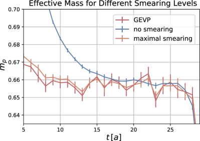
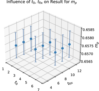
Figure 2: Visualisations for the generalised eigenvalue problem for the $D_{s}$ at rest on E5. Left: Effective mass for the smearings [0,0],[80,80] and the GEVP projection. Right: Result of the mass extraction with consistent plateau ranges for different GEVP parameters.

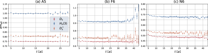
Figure 3: Effective masses obtained from the projected 2-pt. correlators $\tilde{C}^{0,D_{s}}$, $\tilde{C}^{0,D^{*}_{s}}$ and $\tilde{C}^{H_{s}(3)}$, together with the extracted mass. The data correspond to the ensemble A5 (a), F6 (b) and N6 (c).

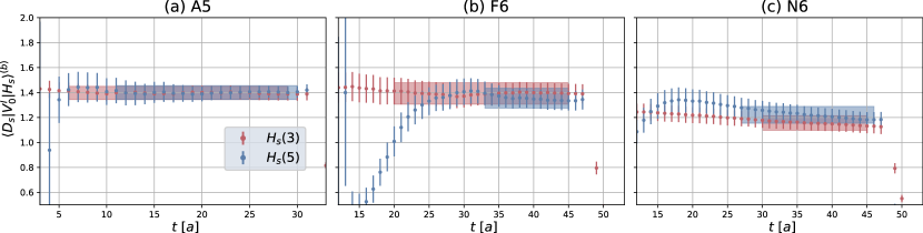
Figure 4: Bare hadronic matrix element $\langle D_{s}(\theta)|V^{I}_{0}|H_{s}(i=\{3,5\})\rangle$ extracted from the fits according to eq. (3.33). The data correspond to the ensemble A5, $\theta=0.525\pi/32$ (a), F6, $\theta=0.65625\pi/48$ (b) and N6, $\theta=0.887\pi/48$ (c).

Figure 5: Bare hadronic matrix element $\langle D_{s}(\theta)|\vec{V}^{I}|H_{s}(i=\{3,5\})\rangle^{(b)}$ extracted from the fits according to eq. (3.33). The data correspond to the ensemble A5, $\theta=0.525\pi/32$ (a), F6, $\theta=0.65625\pi/48$ (b) and N6, $\theta=0.887\pi/48$ (c).

Figure 6: Bare hadronic matrix element $\langle D^{*}_{s}(\theta)|\vec{A}|H_{s}(i=\{3,5\})\rangle^{(b)}_{\parallel}$ extracted from the fits according to eq. (3.33). The data correspond to the ensemble A5, $\theta=0.525\pi/32$ (a), F6, $\theta=0.65625\pi/48$ (b) and N6, $\theta=0.887\pi/48$ (c).

In more detail, the extraction of the matrix elements involves the following elements

• We apply symmetries, solve the GEVP and project the correlators following eq. (3.31).

• The masses and energies, $am_{H_{s}}$ and $aE_{D_{s}^{(*)}}$, are extracted from a plateau of the effective mass of the projected correlator.

• The amplitudes ${\cal Z}^{\theta,H_{s}}$ and ${\cal Z}^{\theta,D^{(*)}_{s}}$ are obtained from a fit with eq. (3.32).

• We divide the three-point-correlator by $\frac{\sqrt{{\cal Z}^{\theta,H_{s}}{\cal Z}^{\theta,D^{(*)}_{s}}}}{2m_{H_{s}}E_{D_{s}^{(*)}}}e^{-E_{D_{s}^{(*)}}\frac{T}{2}}e^{-(m_{B_{s}}-E_{D_{s}^{(*)}})t}$ and fit the resulting plateau to get $\langle D_{s}(\theta)|V^{I}_{\mu}|H_{s}\rangle^{(b)}$ or $R^{(b)}_{kk}$ (eq. (3.33) without the backward contributions in time.)

Figures 3 – 6 display some effective masses of pseudoscalar and vector heavy-strange mesons and hadronic matrix elements. Raw data are collected in the appendix.

4.2 Extrapolation to the physical point

Once we have obtained the hadronic matrix elements, we are in principle able to determine the heavy quark symmetry form factors $h^{+}$, $h^{-}$ and $h_{A_{1,3}}$. Unfortunately the statistical quality of our data is not sufficient to reliably calculate $h_{A_{3}}$. Therefore we will restrict ourselves to the two former quantities at non zero recoil and on $h_{A_{1}}(w=1)$. We have tried to extrapolate $h^{+}$ and $h^{-}$ to $w=1$ separately, and compute ${\cal G}(1)$ from it, as well as to extrapolate ${\cal G}(w)$ directly. The two extrapolations are mostly compatible, because the range in $w$ is very small. We have performed linear and quadratic extrapolations in $(w-1)$. As quadratic fit coefficients are consistent with zero for almost all ensembles, we work with the result from the linear extrapolations for the remainder of the analysis. In Figure 7 we show extrapolations of ${\cal G}$ to zero recoil for a selection of ensembles.

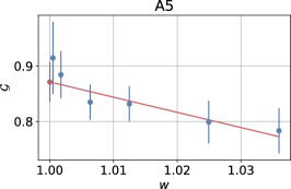
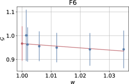
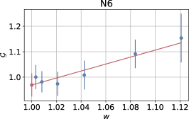
Figure 7: Linear extrapolation of ${\cal{G}}(w)$ to the point of zero recoil ($w=1$). Examples given for three ensembles at $m_{H_{s}}=\lambda^{2}m_{D_{s}}$.

The next-to-last step is to extrapolate $\Sigma^{i}_{\cal G}=\frac{{\cal G}(1,a,m^{2}_{\pi},m_{H_{s}(i)})}{{\cal G}(1,a,m^{2}_{\pi},m_{H_{s}(i-1)})}$ to the physical point, where $i$ denotes the mass step-scaling step corresponding to $m_{H_{s}(i)}=\lambda^{i}m_{D_{s}}$. We have used the following fit ansatz:

$$\Sigma^{i}_{\cal G}(w=1,a,m^{2}_{\pi})=\Sigma^{i}_{{\cal G},0}+\Sigma^{i}_{{\cal G},1}\times(a/a_{\beta=5.3})^{2}+\Sigma^{i}_{{\cal G},2}\times\left(\frac{m_{\pi}}{m^{\rm physical}_{\pi}}\right)^{2}.$$ (4.36)

The fit parameters and $\chi^{2}/d.o.f.$ are collected in Table 3.

i	$\Sigma^{i}_{{\cal G},0}$	$\Sigma^{i}_{{\cal G},1}$	$\Sigma^{i}_{{\cal G},2}$	$\chi^{2}/d.o.f.$
1	1.018(32)	-0.033(24)	0.0006(32)	0.46924
2	1.005(25)	-0.019(18)	0.0000(27)	0.35307
3	1.011(35)	0.044(40)	-0.0057(43)	0.56284
4	0.993(33)	0.033(25)	-0.0028(29)	0.91723
5	1.007(63)	-0.010(75)	0.0009(75)	1.09348

Table 3: Fit parameters for the extrapolation of $\Sigma^{i}_{\cal G}$.

Parametrisations with additional terms were also studied. In particular, one might include a mistuning term $\left(1-\frac{m_{H_{s}}}{\lambda^{i}m_{Ds}}\right)$ to account for the fact that the heavy meson masses are not tuned exactly equally on each ensemble.

However we decided to only include the terms in eq. (4.36)), because the data are so noisy that the fits can not reliably resolve these terms. In fact, as seen in Table 3, only very few non-constant terms are statistically significant. Cut off effects are limited to 5%, while a pion mass dependence is almost absent. Then, we can write

$$\sigma^{i}_{\cal G}(m^{2,\,{\rm physical}}_{\pi})=\Sigma^{i}_{\cal G}(w=1,a=0,m^{2}_{\pi}=m^{2,\,{\rm physical}}_{\pi})=\Sigma^{i}_{{\cal G}_{0}}+\Sigma^{i}_{{\cal G}_{2}}.$$ (4.37)

Unfortunately, no clear trend in $m_{H_{s}}$ dependence is seen, as shown in the left panel of Figure 8. That is why we have fitted the ratios $\sigma^{i}_{\cal G}$ by a constant $\overline{\sigma}_{\cal G}$. We get ${\overline{\sigma}_{\cal G}=1.005(23)}$.

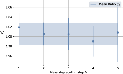
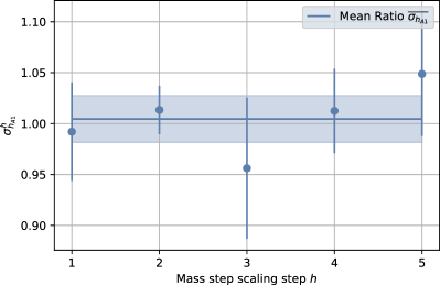
Figure 8: Average ratio of successive $\cal G$ (left) and $h_{A_{1}}$ (right) at the physical point.

Moreover, we have checked, whether our data obey the constraint ${{\cal G}(1,m_{D_{s}})=1}$. To do so, we have performed the following extrapolation:

$${\cal G}(1,a,m^{2}_{\pi},m_{D_{s}})={\cal G}_{0}+{\cal G}_{1}\times(m^{2}_{\pi}/m^{2,{\rm physical}}_{\pi})+{\cal G}_{2}\times(a/a_{\beta=5.3})^{2}.$$ (4.38)

The left panel of Figure 9 shows that our continuum extrapolation ${\cal G}(1,m_{D_{s}})$ is fully compatible with 1 within the limited statistics.

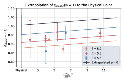
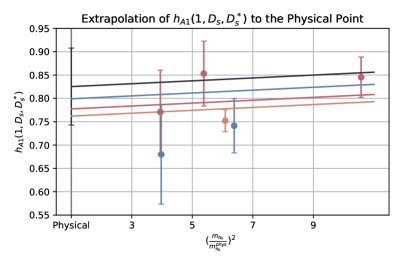
Figure 9: Visualisation of the combined fit eq. (4.38) and extrapolation to the physical point for $\cal{G}_{\mathrm{elastic}}$ (left) and $h_{A_{1}}(D_{s},D_{s}^{*})$ (right).

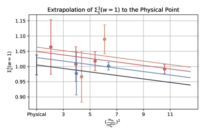
Figure 10: Visualisation of the extrapolation to the physical point of the ratio $\Sigma^{i}_{\cal{G}}(w=1)$ using eq. (4.36) for two different mass step-scaling steps.

As a final result for ${\cal G}$ we quote

$${\cal G}^{B_{s}\to D_{s}}(w=1)=\overline{\sigma}_{\cal G}^{K}=\overline{\sigma}_{\cal G}^{6}=1.03(14).$$ (4.39)

We have also performed a combined fit for the ratio using all data points simultaneously to explore the mass dependence and the effects of mistuning between the different ensembles:

$$\Sigma_{\cal G}(w=1,a,m_{\pi},m_{H_{s}}) = \Sigma_{{\cal G}_{0}}+\Sigma_{{\cal G}_{1}}\times(a/a_{\beta=5.3})^{2}+\Sigma_{{\cal G}_{2}}\times\left(\frac{m_{\pi}}{m^{physical}_{\pi}}\right)^{2}$$ (4.40)

$$+ \Sigma_{{\cal G}_{3}}\times(r_{\rm mis}-1)+\Sigma_{{\cal G}_{4}}\times\frac{m_{B_{s}}}{m_{H_{s}}},$$

where $r_{\rm mis}$ is defined as $\frac{am_{H_{s}}}{\lambda^{i}am_{Ds}}$ and $m_{H_{s}}$ denotes the physical meson mass. While the mistuning is not significant, $\Sigma_{{\cal G}_{3}}=0.69(71)$, an inclusion of this term makes the fit less stable. The last term does contribute $\Sigma_{{\cal G}_{4}}=-0.0248(91)$, but the ratios (analogous to Figure 8) are still compatible with a constant. We obtain a final result for this method by computing

$$\prod\limits_{h=1}^{6}\Sigma_{\cal G}(w=1,a=0,m_{\pi}=m_{\pi}^{\rm phys},m_{Ds}\lambda^{i})=1.03(14).$$ (4.41)

Coincidently we get the same result as we get with the individual fits.

The extrapolation of $h_{A_{1}}$ to the physical point is completely analogous to that of ${\cal G}$. We have decided to use individual fits as we did for the extrapolation of $G$. First we use the ansatz

$${h_{A_{1}}}^{\rm lat}(w=1,a,m^{2}_{\pi},m_{D_{s}})={h^{0}_{A_{1}}}+{h^{1}_{A_{1}}}(m_{\pi}/m^{{\rm physical}}_{\pi})^{2}+{h^{2}_{A_{1}}}(a/a_{\beta=5.3})^{2}$$ (4.42)

to get ${h^{D_{s}\to D^{*}_{s}}_{A_{1}}}(1)$ as shown in the right panel of Figure 9. Then the ratios of successive mass-step-scaling steps are fitted with

$$\Sigma^{i}_{h_{A_{1}}}(1,a,m^{2}_{\pi})=\Sigma^{i,0}_{{h_{A_{1}}}}+\Sigma^{i,1}_{{h_{A_{1}}}}\times(a/a_{\beta=5.3})^{2}+\Sigma^{i,2}_{{h_{A_{1}}}}\times\left(\frac{m_{\pi}}{m^{\rm physical}_{\pi}}\right)^{2}.$$ (4.43)

The fit results are listed in Table 4.

$i$	$\Sigma^{i,0}_{{h_{A_{1}}}}$	$\Sigma^{i,1}_{{h_{A_{1}}}}$	$\Sigma^{i,2}_{{h_{A_{1}}}}$	$\chi^{2}/d.o.f.$
1	0.993(50)	-0.002(38)	-0.0011(24)	0.56485
2	1.015(26)	-0.007(19)	-0.0018(26)	0.47967
3	0.958(72)	0.081(74)	-0.0022(63)	1.08455
4	1.013(44)	0.008(31)	-0.0005(39)	0.11045
5	1.038(66)	-0.125(90)	0.010(10)	0.26381

Table 4: Fit parameters for the extrapolation of $\Sigma^{i}_{h_{A_{1}}}$.

Again, the pion mass dependence is very weak, below 1%. It is less straightforward to conclude about cut off effects. They seem to be more significant than for $\Sigma^{i}_{\cal G}$, as large as 12%. As for $\Sigma^{i}_{\cal G}$, adding a mistuning term $\left(1-\frac{m_{H_{s}}}{\lambda^{i}m_{D_{s}}}\right)$ has made the fits unstable. In the same way as before, from the ratios at the physical point and in the continuum limit, a fit to a constant $\overline{\sigma}_{h_{A_{1}}}$ of the ratios $\sigma^{i}_{h_{A_{1}}}$ is performed, because again no clear trend in $m_{H_{s}}$ is observed as shown in the right panel of Figure 8. The result for $h_{A_{1}}$ can now be calculated according to eq. (2.24)

$$h^{B_{s}\to D^{*}_{s}}_{A_{1}}(1)=h^{D_{s}\to D^{*}_{s}}_{A_{1}}(1)\times(\overline{\sigma}_{{h}_{A_{1}}})^{K}=0.825(83)\times(1.005(23))^{6}=0.85(16).$$ (4.44)

4.3 Discussion

To our knowledge, only three lattice results for ${\cal G}^{B_{s}\to D_{s}}(1)$ are quoted in the literature. The ETM Collaboration, in their analysis of ensembles with ${N}_{f}=2$ twisted-mass fermions, gets ${\cal G}^{B_{s}\to D_{s}}(1)=1.052(46)$, using the step-scaling in mass method defined through RGI quark masses [20]. The HPQCD Collaboration has analysed ensembles with ${N}_{f}=2+1$ staggered fermions, using the non-relativistic framework to regularise the $b$ quark. The result reads ${\cal G}^{B_{s}\to D_{s}}(1)=1.068(40)$ [21]. They have also analysed ensembles with ${N_{f}=2+1+1}$ staggered fermions, regularising the $b$ quark with the heavy HISQ action [24]: they get ${\cal G}^{B_{s}\to D_{s}}(1)=1.070(42)$. Our result is in the same ballpark as the three previous lattice computations, with a significantly larger error. A possible explanation is that we have set a large source-sink time separation $\raisebox{-2.58334pt}{$\stackrel{{\scriptstyle\textstyle{>}}}{{\sim}}$}\,2$ fm. This conservative choice helps to reduce the contamination from excited states with the caveat that the signal deteriorates faster for correlators build from heavy quarks.

Let us emphasize that a gain in statistics at each individual point of the step-scaling in mass strategy would have a significant impact to reduce the error on the final result, because the individual errors multiply with each other along the steps.

Three lattice results have been quoted in the literature for $h^{B_{s}\to D^{*}_{s}}_{A_{1}}(1)$ by HPQCD Collaboration at ${N_{f}}=2+1$ and ${N_{f}=2+1+1}$. Using non-relativistic $b$ quark, again, they get $h^{B_{s}\to D^{*}_{s}}_{A_{1}}(1)=0.883(40)$ [22] while, in the heavy HISQ framework, they get $h^{B_{s}\to D^{*}_{s}}_{A_{1}}(1)=0.9020(96)(90)$ [23] by a measurement direcly at zero recoil and $h^{B_{s}\to D^{*}_{s}}_{A_{1}}=0.875(45)$ [25] by extrapolation to zero recoil. the authors of [22] find a tiny dependence on the spectator quark mass ($h^{B\to D^{*}}_{A_{1}}/h^{B_{s}\to D^{*}_{s}}_{A_{1}}=1.013(31)$). The FNAL/MILC Collaboration finds from another set of ensembles with ${N_{f}=2+1}$ staggered fermions, $h^{B\to D^{*}}_{A_{1}}(1)=0.906(20)$, using the Fermilab action to regularize the $b$ quark [39]. Two more recent preliminaries studies by this collaboration state $h^{B\to D^{*}}_{A_{1}}(1)\in[0.90,0.95]$ [40, 41]. Thus there convincing evidence that $h^{B_{s}\to D^{*}_{s}}_{A_{1}}(1)\sim 0.9$. The same remark concerning our statistical error can be made for $h^{B_{s}\to D^{*}_{s}}_{A_{1}}$ as we did for ${\cal G}^{B_{s}\to D_{s}}(1)$ . The value of the “elastic" point $h^{D_{s}\to D^{*}_{s}}_{A_{1}}(1)$ leads to the conclusion that heavy quark mass dependence on this form factor is smaller than 10%, as it is for ${\cal G}^{H_{s}\to D_{s}}(1)$.

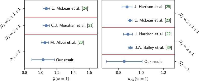
Figure 11: Comparison to previous results for $\mathcal{G}(w=1)$ (left) and $h_{{\rm A}_{1}}$ (right).

5 Conclusion

In the present paper we have reported an ${N_{f}=2}$ lattice QCD computation of the form factors ${\cal G}(1)$ and $h_{A_{1}}(1)$ associated to the $B_{s}\to D^{(*)}_{s}l\nu$ semileptonic decays. For the purpose of extracting the underlying heavy-heavy hadronic matrix elements from suitable correlators, we have clearly demonstrated that solving the GEVP is beneficial to reduce their contamination by excited states. Yet, only smearing $D^{(*)}_{s}$ and $B_{s}$ interpolating fields is already a good starting point. Step-scaling in masses helps to control cut-off effects originating from the heavy quark regularised on the lattice with the Wilson-Clover action. The twisted-boundary condition technique proves to be very helpful to extrapolate ${\cal G}(w)$ at zero recoil. It allows us to consider kinematics near-zero recoil so that a linear extrapolation in $(w-1)$ is fully satisfactory. As we were conservative in setting the source-sink time separation larger than 2 fm in 3pt. correlation functions, we end up with statistical errors $\sim 2.5\%$ in the heavy-strange meson masses sequence of form factor ratios. This precision is not yet sufficient to be sensitive to the heavy quark mass dependence and thus also entails the still considerably large overall errors of the form factors from the present pilot study.

From the findings of our study, it can be deduced that a significant improvement in precision can be expected from a reduced, less conservative choice for the source-sink time separation and focusing on the most smeared sources, on top of generally higher statistics of the individual ensembles of gauge field configurations that enter the analysis. However, rather than pursuing this for the two-flavour theory which is known to have only limited impact on precision phenomenology, we intend to take these aspects into account in a future calculation of $B_{s}\to D_{s}^{(*)}$ form factors using lattice QCD ensembles with $N_{f}=2+1$ dynamical quarks in the medium term. In fact, thanks again to large-scale simulations carried out by the CLS (Coordinated Lattice Simulations) cooperation of researchers, a rich landscape of such $(2+1)$-flavour gauge field configuration ensembles is already available [42, 43, 44], which are to be regarded as natural successors to the ones investigated in the present work. These ensembles employ non-perturbatively ${O}(a)$ improved Wilson-Clover fermions, together with the tree-level Symanzik-improved gauge action, and cover lattice spacings close to the continuum limit as well as the physical pion mass point. Since they also offer statistics substantially higher than underlying our $N_{f}=2$ analysis, a computationally feasible application of the methods studied (and its extensions suggested) here to the $N_{f}=2+1$ case, including additional form factors of the $B_{s}$ system, now appears realistic. Therefore, even though the cost of large-volume calculations via the step-scaling in mass strategy remains challenging, an outcome of phenomenologically interesting target precision of a few percent may be accomplished from this approach on a reasonable time scale.

Finally, let us also mention the recently proposed, so-called stabilised Wilson fermions as a new avenue for QCD calculations with (improved) Wilson-type fermions [45]. First simulations of lattice QCD with $2+1$ dynamical quark flavours within this formulation [46], which amounts to replace the original clover term with an exponentiated version of it, already hint at improved properties such as, apart from stabilising simulations in large volumes towards small pion masses, an overall good continuum scaling and milder relative quark mass dependent cutoff effects. Hence, this framework brings into sight another promising direction for estimating strong interaction effects in precision weak interaction phenomenology through lattice QCD that we are also envisaging for future applications of the techniques explored in the present study.

Appendix

Here we collect the raw data (masses, hadronic matrix elements and form factors) from our analysis.

$\kappa_{h}$	range	$am_{p}$
0.12531	[8,24]	0.74953(64)
0.121364	[8,22]	0.88547(91)
0.11604	[6,20]	1.04906(68)
0.109307	[7,25]	1.23385(71)
0.100407	[8,20]	1.45746(88)
0.089288	[6,17]	1.71981(79)

Table 5: Pseudoscalar masses on A5.

$\kappa_{h}$	$\theta$	range	$V_{0}^{I}$	$V_{0}^{IR}$	range	$V_{n}^{I}$	$V_{n}^{IR}$
0.12531	0	[8, 29]	1.353(27)	1.315(26)	[17, 29]	0.0032(15)	0.0031(15)
0.12531	0.15	[5, 28]	1.392(48)	1.352(47)	[15, 29]	0.0185(55)	0.0180(53)
0.12531	0.3	[6, 28]	1.385(47)	1.345(46)	[10, 32]	0.0263(45)	0.0255(44)
0.12531	0.525	[6, 27]	1.336(46)	1.298(44)	[10, 31]	0.0443(47)	0.0430(46)
0.12531	0.75	[7, 27]	1.327(49)	1.290(47)	[10, 30]	0.0631(53)	0.0613(52)
0.12531	1.05	[5, 26]	1.295(53)	1.258(52)	[18, 31]	0.0859(73)	0.0834(71)
0.12531	1.275	[6, 28]	1.281(57)	1.245(56)	[12, 30]	0.1043(78)	0.1014(76)
0.121364	0	[5, 26]	1.385(29)	1.407(29)	[17, 30]	0.0029(14)	0.0030(14)
0.121364	0.15	[6, 29]	1.424(53)	1.446(54)	[11, 29]	0.0172(50)	0.0175(51)
0.121364	0.3	[9, 30]	1.413(50)	1.436(50)	[8, 28]	0.0306(52)	0.0311(53)
0.121364	0.525	[8, 28]	1.373(50)	1.395(51)	[11, 31]	0.0441(50)	0.0448(50)
0.121364	0.75	[7, 28]	1.364(53)	1.386(54)	[10, 30]	0.0640(57)	0.0650(58)
0.121364	1.05	[5, 27]	1.315(60)	1.336(61)	[9, 29]	0.0904(69)	0.0919(70)
0.121364	1.275	[3, 27]	1.301(63)	1.322(64)	[11, 30]	0.1089(81)	0.1107(82)
0.11604	0	[7, 29]	1.400(30)	1.513(33)	[16, 31]	0.0031(14)	0.0033(15)
0.11604	0.15	[4, 29]	1.440(58)	1.555(63)	[9, 28]	0.0178(53)	0.0192(58)
0.11604	0.3	[17, 31]	1.419(49)	1.533(53)	[10, 27]	0.0319(60)	0.0344(64)
0.11604	0.525	[6, 29]	1.397(53)	1.508(57)	[13, 30]	0.0433(54)	0.0468(59)
0.11604	0.75	[6, 29]	1.386(56)	1.497(60)	[11, 30]	0.0640(60)	0.0692(65)
0.11604	1.05	[6, 27]	1.320(67)	1.425(73)	[10, 29]	0.0935(75)	0.1009(81)
0.11604	1.275	[6, 29]	1.301(72)	1.405(78)	[12, 28]	0.1113(92)	0.1202(99)
0.109307	0	[7, 28]	1.443(38)	1.687(44)	[11, 28]	0.0050(22)	0.0059(25)
0.109307	0.15	[3, 30]	1.457(65)	1.704(76)	[16, 28]	0.0283(62)	0.0331(73)
0.109307	0.3	[4, 29]	1.449(66)	1.694(77)	[14, 28]	0.0421(64)	0.0492(75)
0.109307	0.525	[6, 29]	1.440(59)	1.684(69)	[11, 31]	0.0470(57)	0.0550(66)
0.109307	0.75	[4, 30]	1.437(61)	1.681(71)	[10, 31]	0.0659(63)	0.0770(74)
0.109307	1.05	[4, 30]	1.428(77)	1.671(91)	[10, 28]	0.0807(82)	0.0944(96)
0.109307	1.275	[6, 30]	1.419(83)	1.659(98)	[10, 28]	0.0962(96)	0.113(11)
0.100407	0	[10, 29]	1.403(35)	1.833(46)	[12, 28]	0.0055(21)	0.0072(27)
0.100407	0.15	[9, 30]	1.415(62)	1.848(80)	[14, 29]	0.0268(59)	0.0351(77)
0.100407	0.3	[10, 30]	1.404(61)	1.833(80)	[14, 29]	0.0396(62)	0.0518(81)
0.100407	0.525	[11, 30]	1.399(55)	1.828(72)	[10, 30]	0.0466(61)	0.0609(80)
0.100407	0.75	[10, 30]	1.398(58)	1.826(76)	[9, 31]	0.0661(63)	0.0863(82)
0.100407	1.05	[10, 29]	1.406(78)	1.84(10)	[10, 27]	0.0771(90)	0.101(12)
0.100407	1.275	[10, 31]	1.400(84)	1.83(11)	[11, 28]	0.094(10)	0.123(14)
0.089288	0	[13, 29]	1.309(30)	1.988(46)	[15, 32]	0.0030(14)	0.0046(21)
0.089288	0.15	[16, 30]	1.332(48)	2.023(72)	[13, 27]	0.0103(74)	0.016(11)
0.089288	0.3	[14, 28]	1.332(53)	2.023(81)	[13, 29]	0.0190(60)	0.0288(91)
0.089288	0.525	[16, 30]	1.350(53)	2.051(81)	[18, 29]	0.0395(62)	0.0600(95)
0.089288	0.75	[17, 32]	1.347(54)	2.046(82)	[12, 29]	0.0628(70)	0.095(11)
0.089288	1.05	[17, 31]	1.228(57)	1.866(87)	[13, 30]	0.0872(74)	0.132(11)
0.089288	1.275	[18, 30]	1.214(65)	1.843(98)	[11, 29]	0.1009(93)	0.153(14)

Table 6: Improved and renormalised hadronic matrix elements $\langle D_{s}|V_{\mu}|H_{s}\rangle$ on A5.

$\kappa_{h}$	range	$\langle D_{s}^{*}|\vec{A}^{I}|H_{s}\rangle^{R}_{\parallel}$	$h_{A_{1}}$	$\Sigma_{h_{A1}}$
0.12531	[6, 24]	1.204(38)	0.752(24)	-
0.121364	[7, 25]	1.229(44)	0.739(26)	0.983(12)
0.11604	[7, 23]	1.247(51)	0.732(30)	0.991(11)
0.109307	[8, 27]	1.400(64)	0.820(37)	1.121(65)
0.100407	[11, 27]	1.391(74)	0.838(45)	1.022(14)
0.089288	[19, 31]	1.206(81)	0.777(52)	0.928(75)

Table 7: $h_{A_{1}}$ extracted on ensemble A5.

Scaling Step	$\mathcal{G}(w=1)$	$\Sigma_{\mathcal{G}}$
$D_{s}$	0.872(17)	-
1	0.862(23)	0.9890(10)
2	0.848(26)	0.98289(81)
3	0.923(39)	1.0893(29)
4	0.932(48)	1.00921(92)
5	0.850(51)	0.9124(46)

Table 8: $\mathcal{G}$ at zero recoil and $\Sigma_{i}=\frac{\mathcal{G}_{i}}{\mathcal{G}_{i-1}}$ on A5.

$\kappa_{h}$	range	$am_{p}$
0.12529	[11,37]	0.74884(34)
0.121313	[11,37]	0.88526(48)
0.116844	[12,34]	1.02281(57)
0.109127	[8,27]	1.23825(51)
0.100172	[7,23]	1.46300(53)
0.088934	[8,20]	1.72617(57)

Table 9: Pseudoscalar masses on B6.

$\kappa_{h}$	$\theta$	range	$V_{0}^{I}$	$V_{0}^{IR}$	range	$V_{n}^{I}$	$V_{n}^{IR}$
0.12529	0	[9, 40]	1.406(48)	1.367(47)	[14, 45]	0.0045(19)	0.0044(19)
0.12529	0.163	[7, 44]	1.424(46)	1.384(45)	[12, 46]	0.0091(37)	0.0089(36)
0.12529	0.326	[9, 44]	1.425(41)	1.386(40)	[9, 46]	0.0169(61)	0.0164(60)
0.12529	0.5705	[6, 42]	1.403(52)	1.364(51)	[14, 48]	0.0270(70)	0.0262(68)
0.12529	0.815	[7, 40]	1.398(53)	1.359(52)	[12, 47]	0.0377(68)	0.0367(66)
0.12529	1.14095	[15, 45]	1.369(53)	1.331(51)	[9, 43]	0.0713(73)	0.0693(71)
0.12529	1.38545	[13, 45]	1.361(53)	1.323(51)	[15, 42]	0.0844(83)	0.0821(81)
0.121313	0	[8, 41]	1.433(54)	1.458(55)	[14, 45]	0.0059(28)	0.0060(28)
0.121313	0.163	[10, 44]	1.454(50)	1.478(51)	[15, 46]	0.0113(54)	0.0115(55)
0.121313	0.326	[7, 44]	1.455(47)	1.480(48)	[14, 46]	0.0186(72)	0.0189(74)
0.121313	0.5705	[9, 42]	1.434(55)	1.458(56)	[15, 46]	0.0272(75)	0.0277(77)
0.121313	0.815	[7, 43]	1.430(59)	1.454(60)	[9, 45]	0.0376(75)	0.0383(77)
0.121313	1.14095	[15, 45]	1.393(61)	1.417(62)	[10, 44]	0.0757(88)	0.0769(89)
0.121313	1.38545	[21, 46]	1.373(71)	1.396(73)	[9, 43]	0.0895(98)	0.0910(100)
0.116844	0	[16, 44]	1.440(57)	1.556(62)	[20, 45]	0.0073(34)	0.0079(37)
0.116844	0.163	[16, 44]	1.465(54)	1.583(58)	[22, 43]	0.0134(89)	0.0145(96)
0.116844	0.326	[16, 45]	1.467(50)	1.585(54)	[20, 45]	0.022(10)	0.024(11)
0.116844	0.5705	[14, 45]	1.444(59)	1.560(64)	[19, 46]	0.0284(77)	0.0307(83)
0.116844	0.815	[15, 44]	1.440(65)	1.555(71)	[17, 45]	0.0391(92)	0.0423(99)
0.116844	1.14095	[18, 46]	1.399(72)	1.511(77)	[17, 44]	0.078(10)	0.084(11)
0.116844	1.38545	[21, 45]	1.384(82)	1.495(89)	[15, 42]	0.091(12)	0.098(13)
0.109127	0	[21, 45]	1.393(48)	1.633(56)	[24, 46]	0.0033(24)	0.0039(28)
0.109127	0.163	[29, 46]	1.402(49)	1.644(57)	[29, 47]	0.0047(49)	0.0055(58)
0.109127	0.326	[25, 45]	1.392(52)	1.632(61)	[26, 45]	0.0123(85)	0.0144(99)
0.109127	0.5705	[21, 46]	1.402(54)	1.644(64)	[24, 48]	0.0395(77)	0.0464(90)
0.109127	0.815	[22, 45]	1.402(61)	1.644(71)	[28, 47]	0.0529(89)	0.062(10)
0.109127	1.14095	[26, 45]	1.382(67)	1.621(79)	[15, 39]	0.056(15)	0.065(18)
0.109127	1.38545	[31, 45]	1.378(74)	1.616(87)	[20, 43]	0.070(13)	0.082(16)
0.100172	0	[25, 47]	1.356(44)	1.781(58)	[29, 48]	0.0037(25)	0.0049(32)
0.100172	0.163	[31, 46]	1.370(47)	1.799(62)	[32, 47]	0.0069(56)	0.0091(73)
0.100172	0.326	[27, 46]	1.359(51)	1.785(66)	[24, 41]	0.017(13)	0.022(17)
0.100172	0.5705	[25, 46]	1.371(53)	1.800(70)	[28, 48]	0.0418(81)	0.055(11)
0.100172	0.815	[25, 46]	1.369(60)	1.798(79)	[29, 47]	0.0536(91)	0.070(12)
0.100172	1.14095	[26, 45]	1.355(69)	1.780(90)	[24, 43]	0.052(13)	0.069(17)
0.100172	1.38545	[33, 46]	1.346(73)	1.768(96)	[25, 45]	0.073(12)	0.096(16)
0.088934	0	[29, 46]	1.291(40)	1.982(61)	[30, 48]	0.0022(23)	0.0034(35)
0.088934	0.163	[31, 45]	1.324(44)	2.032(67)	[28, 45]	0.0156(97)	0.024(15)
0.088934	0.326	[32, 46]	1.328(44)	2.038(67)	[26, 40]	0.025(13)	0.039(19)
0.088934	0.5705	[32, 45]	1.311(54)	2.013(83)	[34, 49]	0.0245(73)	0.038(11)
0.088934	0.815	[33, 46]	1.308(57)	2.009(87)	[36, 47]	0.0398(83)	0.061(13)
0.088934	1.14095	[37, 47]	1.183(59)	1.816(90)	[21, 40]	0.072(22)	0.110(33)
0.088934	1.38545	[37, 47]	1.149(72)	1.76(11)	[29, 46]	0.076(13)	0.117(20)

Table 10: Improved and renormalised hadronic matrix elements $\langle D_{s}|V_{\mu}|H_{s}\rangle$ on B6.

Scaling Step	$\mathcal{G}(w=1)$	$\Sigma_{\mathcal{G}}$
$D_{s}$	0.925(30)	-
1	0.895(41)	0.96727(89)
2	0.878(53)	0.98133(78)
3	0.848(60)	0.9664(31)
4	0.895(76)	1.0551(10)
5	0.847(89)	0.9459(45)

Table 11: $\mathcal{G}$ at zero recoil and $\Sigma_{i}=\frac{\mathcal{G}_{i}}{\mathcal{G}_{i-1}}$ on B6.

$\kappa_{h}$	range	$am_{p}$
0.12724	[9,25]	0.65743(80)
0.123874	[8,27]	0.7765(10)
0.119457	[9,27]	0.9166(11)
0.113638	[7,27]	1.0835(12)
0.106031	[7,22]	1.2813(13)
0.0965545	[8,17]	1.5084(16)

Table 12: Pseudoscalar masses on E5.

$\kappa_{h}$	$\theta$	range	$V_{0}^{I}$	$V_{0}^{IR}$	range	$V_{n}^{I}$	$V_{n}^{IR}$
0.12724	0	[5, 29]	1.325(43)	1.261(41)	[7, 32]	0.0037(20)	0.0035(19)
0.12724	0.125	[7, 27]	1.331(41)	1.266(40)	[5, 29]	0.0115(39)	0.0110(37)
0.12724	0.25	[5, 27]	1.340(42)	1.275(40)	[8, 29]	0.0232(41)	0.0221(39)
0.12724	0.4375	[6, 28]	1.365(43)	1.299(41)	[5, 30]	0.0427(44)	0.0407(42)
0.12724	0.625	[4, 29]	1.403(45)	1.335(43)	[9, 27]	0.0609(52)	0.0580(49)
0.12724	0.875	[4, 30]	1.465(51)	1.394(48)	[11, 30]	0.0863(65)	0.0821(62)
0.12724	1.0625	[5, 28]	1.528(56)	1.454(53)	[12, 29]	0.1078(75)	0.1026(71)
0.123874	0	[5, 28]	1.368(46)	1.354(46)	[4, 30]	0.0040(21)	0.0039(21)
0.123874	0.125	[5, 26]	1.374(45)	1.360(45)	[10, 32]	0.0108(42)	0.0107(41)
0.123874	0.25	[6, 28]	1.384(45)	1.369(44)	[5, 28]	0.0253(48)	0.0250(47)
0.123874	0.4375	[4, 28]	1.409(46)	1.394(46)	[7, 28]	0.0446(52)	0.0441(52)
0.123874	0.625	[4, 29]	1.449(48)	1.433(48)	[9, 28]	0.0642(59)	0.0635(58)
0.123874	0.875	[4, 28]	1.513(55)	1.497(54)	[10, 29]	0.0912(70)	0.0902(69)
0.123874	1.0625	[5, 27]	1.578(60)	1.561(59)	[12, 30]	0.1128(78)	0.1116(77)
0.119457	0	[5, 29]	1.397(52)	1.454(54)	[10, 31]	0.0033(26)	0.0035(28)
0.119457	0.125	[5, 28]	1.404(50)	1.461(52)	[12, 29]	0.0109(47)	0.0113(49)
0.119457	0.25	[5, 27]	1.414(51)	1.472(53)	[12, 30]	0.0242(47)	0.0252(49)
0.119457	0.4375	[5, 30]	1.439(51)	1.497(53)	[7, 29]	0.0461(56)	0.0480(58)
0.119457	0.625	[5, 30]	1.480(54)	1.540(56)	[12, 29]	0.0663(62)	0.0690(65)
0.119457	0.875	[4, 29]	1.545(62)	1.608(64)	[10, 29]	0.0953(75)	0.0992(78)
0.119457	1.0625	[5, 28]	1.613(68)	1.678(71)	[14, 30]	0.1192(88)	0.1241(92)
0.113638	0	[8, 29]	1.412(52)	1.572(58)	[10, 31]	0.0034(34)	0.0037(38)
0.113638	0.125	[6, 27]	1.422(54)	1.583(60)	[11, 30]	0.0108(46)	0.0120(51)
0.113638	0.25	[7, 27]	1.431(53)	1.594(60)	[10, 30]	0.0247(49)	0.0275(55)
0.113638	0.4375	[4, 30]	1.454(53)	1.619(60)	[10, 30]	0.0460(56)	0.0512(63)
0.113638	0.625	[4, 28]	1.497(58)	1.667(65)	[12, 29]	0.0685(67)	0.0762(74)
0.113638	0.875	[6, 28]	1.563(65)	1.740(72)	[9, 30]	0.0981(72)	0.1093(80)
0.113638	1.0625	[5, 29]	1.631(72)	1.817(81)	[12, 30]	0.1221(91)	0.136(10)
0.106031	0	[10, 30]	1.396(54)	1.703(65)	[10, 29]	0.0039(44)	0.0047(54)
0.106031	0.125	[11, 29]	1.405(53)	1.713(65)	[12, 30]	0.0108(46)	0.0131(56)
0.106031	0.25	[10, 29]	1.414(54)	1.725(66)	[11, 30]	0.0248(49)	0.0302(60)
0.106031	0.4375	[12, 29]	1.439(54)	1.756(66)	[11, 29]	0.0463(60)	0.0565(73)
0.106031	0.625	[13, 30]	1.480(56)	1.806(69)	[11, 30]	0.0684(66)	0.0835(80)
0.106031	0.875	[11, 30]	1.545(66)	1.884(81)	[11, 30]	0.0986(77)	0.1203(94)
0.106031	1.0625	[12, 29]	1.615(76)	1.970(93)	[11, 30]	0.1232(96)	0.150(12)
0.0965545	0	[14, 29]	1.351(54)	1.858(74)	[13, 30]	0.0037(37)	0.0051(51)
0.0965545	0.125	[14, 30]	1.356(51)	1.866(71)	[10, 29]	0.0102(48)	0.0140(66)
0.0965545	0.25	[14, 31]	1.366(50)	1.879(69)	[8, 26]	0.0226(71)	0.0311(97)
0.0965545	0.4375	[14, 30]	1.391(53)	1.913(73)	[14, 30]	0.0457(55)	0.0629(76)
0.0965545	0.625	[14, 30]	1.432(57)	1.970(78)	[13, 29]	0.0680(70)	0.0936(97)
0.0965545	0.875	[14, 30]	1.492(66)	2.053(90)	[7, 29]	0.0964(85)	0.133(12)
0.0965545	1.0625	[14, 30]	1.560(76)	2.15(10)	[6, 30]	0.1182(99)	0.163(14)

Table 13: Improved and renormalised hadronic matrix elements $\langle D_{s}|V_{\mu}|H_{s}\rangle$ on E5.

$\kappa_{h}$	range	$\langle D_{s}^{*}|\vec{A}^{I}|H_{s}\rangle^{R}_{\parallel}$	$h_{A_{1}}$	$\Sigma_{h_{A1}}$
0.12724	[10, 23]	1.212(63)	0.845(43)	-
0.123874	[8, 20]	1.240(68)	0.828(44)	0.9791(91)
0.119457	[8, 18]	1.271(78)	0.821(50)	0.992(12)
0.113638	[9, 20]	1.310(91)	0.833(57)	1.015(19)
0.106031	[10, 23]	1.32(11)	0.847(67)	1.016(18)
0.0965545	[14, 29]	1.30(11)	0.866(72)	1.023(22)

Table 14: $h_{A_{1}}$ extracted on Ensemble E5.

Scaling Step	$\mathcal{G}(w=1)$	$\Sigma_{\mathcal{G}}$
$D_{s}$	0.961(29)	-
1	0.945(32)	0.9842(11)
2	0.930(39)	0.98338(98)
3	0.922(57)	0.9919(10)
4	0.919(67)	0.9971(11)
5	0.929(81)	1.0100(13)

Table 15: $\mathcal{G}$ at zero recoil and $\Sigma_{i}=\frac{\mathcal{G}_{i}}{\mathcal{G}_{i-1}}$ on E5.

$\kappa_{h}$	range	$am_{p}$
0.12713	[12,39]	0.65756(70)
0.1237	[10,35]	0.77899(69)
0.119241	[10,34]	0.91989(79)
0.113382	[7,27]	1.08818(74)
0.10593	[8,22]	1.28429(94)
0.096211	[5,18]	1.51684(82)

Table 16: Pseudoscalar masses on F6.

$\kappa_{h}$	$\theta$	range	$V_{0}^{I}$	$V_{0}^{IR}$	range	$V_{n}^{I}$	$V_{n}^{IR}$
0.12713	0	[5, 43]	1.335(68)	1.270(65)	[13, 45]	0.0057(33)	0.0054(31)
0.12713	0.1875	[6, 43]	1.344(68)	1.279(65)	[13, 45]	0.0106(58)	0.0100(55)
0.12713	0.375	[9, 44]	1.332(71)	1.268(68)	[16, 44]	0.0230(59)	0.0219(57)
0.12713	0.65625	[12, 44]	1.337(72)	1.272(69)	[15, 44]	0.0424(64)	0.0403(61)
0.12713	0.9375	[15, 44]	1.343(76)	1.278(73)	[17, 41]	0.0635(81)	0.0604(77)
0.12713	1.3125	[17, 46]	1.358(88)	1.293(84)	[15, 44]	0.0881(91)	0.0838(87)
0.12713	1.59375	[23, 46]	1.37(11)	1.31(10)	[14, 45]	0.107(11)	0.102(10)
0.1237	0	[14, 45]	1.383(76)	1.369(75)	[14, 46]	0.0050(25)	0.0050(25)
0.1237	0.1875	[8, 45]	1.398(79)	1.384(78)	[16, 43]	0.0133(65)	0.0132(65)
0.1237	0.375	[13, 44]	1.378(79)	1.364(79)	[15, 42]	0.0271(69)	0.0268(68)
0.1237	0.65625	[14, 45]	1.379(81)	1.365(80)	[16, 41]	0.0482(78)	0.0477(78)
0.1237	0.9375	[24, 46]	1.375(85)	1.361(84)	[14, 43]	0.0671(82)	0.0664(81)
0.1237	1.3125	[23, 44]	1.39(10)	1.371(99)	[16, 45]	0.094(10)	0.0932(100)
0.1237	1.59375	[26, 46]	1.40(12)	1.39(12)	[13, 43]	0.114(12)	0.113(12)
0.119241	0	[20, 44]	1.403(81)	1.462(84)	[20, 48]	0.0056(31)	0.0059(33)
0.119241	0.1875	[16, 44]	1.418(85)	1.478(88)	[20, 42]	0.0176(75)	0.0183(78)
0.119241	0.375	[21, 46]	1.392(83)	1.451(86)	[20, 42]	0.0312(78)	0.0325(81)
0.119241	0.65625	[20, 45]	1.392(87)	1.451(90)	[20, 41]	0.0529(91)	0.0551(95)
0.119241	0.9375	[21, 45]	1.393(93)	1.451(97)	[20, 41]	0.074(10)	0.077(11)
0.119241	1.3125	[23, 46]	1.40(11)	1.46(11)	[19, 43]	0.101(12)	0.105(13)
0.119241	1.59375	[23, 45]	1.41(13)	1.47(13)	[18, 44]	0.120(15)	0.125(16)
0.113382	0	[23, 45]	1.414(81)	1.576(90)	[28, 48]	0.0062(41)	0.0069(46)
0.113382	0.1875	[25, 46]	1.427(81)	1.590(90)	[26, 44]	0.0181(70)	0.0202(78)
0.113382	0.375	[25, 47]	1.399(81)	1.559(90)	[28, 42]	0.0337(85)	0.0376(95)
0.113382	0.65625	[27, 47]	1.398(83)	1.558(93)	[27, 42]	0.0556(97)	0.062(11)
0.113382	0.9375	[26, 45]	1.399(93)	1.56(10)	[28, 44]	0.0747(99)	0.083(11)
0.113382	1.3125	[27, 46]	1.40(11)	1.56(12)	[21, 44]	0.105(14)	0.117(15)
0.113382	1.59375	[27, 45]	1.42(14)	1.58(15)	[36, 47]	0.116(18)	0.130(20)
0.10593	0	[31, 46]	1.337(67)	1.640(82)	[26, 46]	0.0051(22)	0.0063(27)
0.10593	0.1875	[31, 47]	1.361(68)	1.669(83)	[23, 45]	0.0132(57)	0.0162(70)
0.10593	0.375	[29, 46]	1.346(77)	1.651(94)	[35, 45]	0.0282(69)	0.0346(85)
0.10593	0.65625	[33, 45]	1.354(79)	1.661(97)	[34, 48]	0.0462(70)	0.0567(86)
0.10593	0.9375	[34, 47]	1.367(90)	1.68(11)	[24, 46]	0.0634(89)	0.078(11)
0.10593	1.3125	[34, 47]	1.41(11)	1.73(13)	[32, 45]	0.092(14)	0.112(17)
0.10593	1.59375	[35, 47]	1.46(14)	1.79(17)	[36, 46]	0.113(20)	0.138(24)
0.096211	0	[32, 46]	1.359(72)	1.89(10)	[35, 48]	0.0089(57)	0.0124(79)
0.096211	0.1875	[34, 46]	1.380(72)	1.92(10)	[25, 43]	0.0268(85)	0.037(12)
0.096211	0.375	[32, 47]	1.350(74)	1.88(10)	[30, 46]	0.0381(66)	0.0530(92)
0.096211	0.65625	[33, 47]	1.352(77)	1.88(11)	[35, 48]	0.0580(74)	0.081(10)
0.096211	0.9375	[36, 47]	1.355(82)	1.88(11)	[28, 47]	0.0810(96)	0.112(13)
0.096211	1.3125	[36, 46]	1.37(10)	1.90(14)	[36, 48]	0.106(13)	0.147(18)
0.096211	1.59375	[35, 46]	1.39(13)	1.93(18)	[40, 47]	0.125(19)	0.174(26)

Table 17: Improved and renormalised hadronic matrix elements $\langle D_{s}|V_{\mu}|H_{s}\rangle$ on F6.

$\kappa_{h}$	range	$\langle D_{s}^{*}|\vec{A}^{I}|H_{s}\rangle^{R}_{\parallel}$	$h_{A_{1}}$	$\Sigma_{h_{A1}}$
0.12713	[9, 28]	1.22(10)	0.853(70)	-
0.1237	[12, 28]	1.31(14)	0.872(94)	1.022(34)
0.119241	[17, 41]	1.36(19)	0.88(13)	1.010(56)
0.113382	[21, 42]	1.40(23)	0.89(15)	1.013(37)
0.10593	[24, 38]	1.44(23)	0.93(15)	1.04(24)
0.096211	[28, 40]	1.37(27)	0.92(18)	0.99(26)

Table 18: $h_{A_{1}}$ extracted on Ensemble F6.

Scaling Step	$\mathcal{G}(w=1)$	$\Sigma_{\mathcal{G}}$
$D_{s}$	0.966(50)	-
1	0.959(58)	0.9929(10)
2	0.967(72)	1.0084(11)
3	0.984(86)	1.0177(13)
4	0.911(82)	0.9255(40)
5	1.104(98)	1.2121(55)

Table 19: $\mathcal{G}$ at zero recoil and $\Sigma_{i}=\frac{\mathcal{G}_{i}}{\mathcal{G}_{i-1}}$ on F6.

$\kappa_{h}$	range	$am_{p}$
0.12713	[13,37]	0.65511(28)
0.123649	[14,32]	0.77744(47)
0.119196	[11,35]	0.91865(36)
0.11335	[10,29]	1.08532(41)
0.105786	[8,25]	1.28215(44)
0.096689	[7,23]	1.50077(43)

Table 20: Pseudoscalar masses on F7.

$\kappa_{h}$	$\theta$	range	$V_{0}^{I}$	$V_{0}^{IR}$	range	$V_{n}^{I}$	$V_{n}^{IR}$
0.12713	0	[8, 40]	1.272(26)	1.212(25)	[14, 45]	0.0031(16)	0.0030(15)
0.12713	0.1875	[8, 44]	1.254(44)	1.194(42)	[6, 45]	0.0094(29)	0.0089(27)
0.12713	0.375	[9, 43]	1.253(44)	1.194(42)	[24, 39]	0.0213(52)	0.0203(49)
0.12713	0.65625	[8, 43]	1.227(40)	1.169(38)	[23, 43]	0.0307(57)	0.0293(54)
0.12713	0.9375	[7, 41]	1.226(41)	1.168(39)	[18, 45]	0.0471(58)	0.0448(55)
0.12713	1.3125	[11, 43]	1.340(69)	1.276(65)	[9, 43]	0.0804(51)	0.0766(49)
0.12713	1.59375	[13, 45]	1.325(76)	1.262(72)	[12, 39]	0.0971(65)	0.0925(62)
0.123649	0	[13, 40]	1.307(31)	1.295(31)	[12, 45]	0.0035(17)	0.0034(16)
0.123649	0.1875	[5, 44]	1.286(51)	1.274(50)	[22, 43]	0.0117(41)	0.0116(41)
0.123649	0.375	[6, 42]	1.285(51)	1.273(50)	[26, 48]	0.0230(41)	0.0228(40)
0.123649	0.65625	[7, 44]	1.255(48)	1.244(47)	[17, 44]	0.0333(56)	0.0330(56)
0.123649	0.9375	[7, 39]	1.250(51)	1.239(50)	[20, 46]	0.0490(60)	0.0486(59)
0.123649	1.3125	[11, 41]	1.384(85)	1.371(84)	[11, 43]	0.0866(60)	0.0858(59)
0.123649	1.59375	[10, 44]	1.367(94)	1.355(93)	[12, 42]	0.1029(71)	0.1020(71)
0.119196	0	[14, 42]	1.339(33)	1.395(34)	[18, 45]	0.0039(20)	0.0040(21)
0.119196	0.1875	[12, 43]	1.313(55)	1.368(57)	[22, 44]	0.0121(43)	0.0126(45)
0.119196	0.375	[10, 42]	1.312(56)	1.367(58)	[25, 45]	0.0232(46)	0.0242(48)
0.119196	0.65625	[16, 46]	1.291(50)	1.345(52)	[20, 43]	0.0349(57)	0.0364(60)
0.119196	0.9375	[14, 44]	1.291(55)	1.345(57)	[20, 46]	0.0515(60)	0.0536(62)
0.119196	1.3125	[15, 43]	1.420(98)	1.48(10)	[11, 42]	0.0924(73)	0.0963(76)
0.119196	1.59375	[13, 43]	1.40(11)	1.46(11)	[10, 42]	0.1092(84)	0.1138(88)
0.11335	0	[21, 45]	1.305(30)	1.453(34)	[21, 38]	0.0033(34)	0.0037(38)
0.11335	0.1875	[21, 45]	1.349(47)	1.502(53)	[22, 43]	0.0140(55)	0.0156(61)
0.11335	0.375	[20, 44]	1.345(49)	1.498(54)	[23, 45]	0.0250(50)	0.0278(56)
0.11335	0.65625	[23, 45]	1.314(54)	1.463(61)	[24, 45]	0.0437(62)	0.0487(69)
0.11335	0.9375	[19, 44]	1.321(61)	1.470(68)	[21, 46]	0.0610(62)	0.0679(69)
0.11335	1.3125	[18, 44]	1.279(75)	1.424(83)	[16, 36]	0.0828(96)	0.092(11)
0.11335	1.59375	[21, 45]	1.268(81)	1.412(91)	[23, 43]	0.0860(96)	0.096(11)
0.105786	0	[26, 44]	1.294(30)	1.573(37)	[22, 41]	0.0044(37)	0.0053(45)
0.105786	0.1875	[30, 47]	1.328(44)	1.615(54)	[22, 43]	0.0144(58)	0.0175(71)
0.105786	0.375	[30, 46]	1.324(45)	1.609(55)	[24, 45]	0.0254(52)	0.0309(63)
0.105786	0.65625	[22, 45]	1.299(57)	1.579(69)	[25, 45]	0.0459(61)	0.0558(74)
0.105786	0.9375	[22, 45]	1.312(61)	1.596(74)	[23, 44]	0.0641(74)	0.0779(90)
0.105786	1.3125	[23, 45]	1.272(69)	1.546(84)	[19, 35]	0.079(12)	0.097(15)
0.105786	1.59375	[22, 46]	1.259(85)	1.53(10)	[22, 44]	0.085(10)	0.104(12)
0.096689	0	[28, 44]	1.310(30)	1.782(41)	[25, 39]	0.0098(43)	0.0133(58)
0.096689	0.1875	[24, 42]	1.261(65)	1.715(88)	[23, 42]	0.0240(60)	0.0327(82)
0.096689	0.375	[26, 45]	1.254(59)	1.705(80)	[22, 39]	0.0342(74)	0.046(10)
0.096689	0.65625	[27, 45]	1.333(60)	1.813(81)	[23, 38]	0.045(10)	0.061(14)
0.096689	0.9375	[25, 45]	1.353(64)	1.840(88)	[23, 41]	0.0611(87)	0.083(12)
0.096689	1.3125	[24, 39]	1.343(79)	1.83(11)	[24, 41]	0.104(11)	0.142(15)
0.096689	1.59375	[28, 46]	1.305(74)	1.78(10)	[22, 44]	0.113(12)	0.153(16)

Table 21: Improved and renormalised hadronic matrix elements $\langle D_{s}|V_{\mu}|H_{s}\rangle$ on F7.

$\kappa_{h}$	range	$\langle D_{s}^{*}|\vec{A}^{I}|H_{s}\rangle^{R}_{\parallel}$	$h_{A_{1}}$	$\Sigma_{h_{A1}}$
0.12713	[15, 25]	1.175(41)	0.825(29)	-
0.123649	[14, 30]	1.211(52)	0.813(35)	0.985(15)
0.119196	[14, 34]	1.263(67)	0.820(43)	1.009(15)
0.11335	[16, 34]	1.226(83)	0.782(53)	0.954(80)
0.105786	[19, 33]	1.24(10)	0.794(65)	1.015(22)
0.096689	[22, 33]	1.16(14)	0.771(90)	0.97(13)

Table 22: $h_{A_{1}}$ extracted on Ensemble F7.

Scaling Step	$\mathcal{G}(w=1)$	$\Sigma_{\mathcal{G}}$
$D_{s}$	0.929(20)	-
1	0.901(25)	0.9702(11)
2	0.882(30)	0.97820(88)
3	0.889(38)	1.0078(40)
4	0.908(48)	1.0214(10)
5	0.987(72)	1.0875(58)

Table 23: $\mathcal{G}$ at zero recoil and $\Sigma_{i}=\frac{\mathcal{G}_{i}}{\mathcal{G}_{i-1}}$ on F7.

$\kappa_{h}$	range	$am_{p}$
0.1271	[19,45]	0.65660(86)
0.123719	[13,39]	0.77676(98)
0.11926	[13,32]	0.9179(11)
0.113447	[12,33]	1.0843(12)
0.105836	[8,26]	1.28537(91)
0.096143	[5,24]	1.52492(90)

Table 24: Pseudoscalar masses on G8.

$\kappa_{h}$	$\theta$	range	$V_{0}^{I}$	$V_{0}^{IR}$	range	$V_{n}^{I}$	$V_{n}^{IR}$
0.1271	0	[11, 53]	1.31(17)	1.25(16)	[21, 53]	0.0127(62)	0.0121(59)
0.1271	0.25	[9, 54]	1.28(15)	1.22(14)	[9, 51]	0.0242(98)	0.0230(93)
0.1271	0.5	[8, 55]	1.28(15)	1.22(14)	[14, 48]	0.034(13)	0.032(13)
0.1271	0.875	[11, 55]	1.26(15)	1.20(14)	[9, 48]	0.054(13)	0.051(12)
0.1271	1.25	[11, 54]	1.32(16)	1.26(15)	[17, 49]	0.070(16)	0.067(15)
0.1271	1.75	[9, 52]	1.33(16)	1.27(15)	[13, 48]	0.090(21)	0.086(20)
0.1271	2.125	[11, 55]	1.35(18)	1.28(17)	[12, 48]	0.104(23)	0.099(22)
0.123719	0	[18, 53]	1.36(21)	1.35(21)	[22, 56]	0.0129(66)	0.0128(65)
0.123719	0.25	[19, 57]	1.32(18)	1.30(18)	[22, 56]	0.022(12)	0.021(12)
0.123719	0.5	[16, 57]	1.32(18)	1.31(17)	[23, 55]	0.034(14)	0.034(14)
0.123719	0.875	[21, 57]	1.29(18)	1.28(17)	[21, 51]	0.058(16)	0.057(16)
0.123719	1.25	[23, 56]	1.36(18)	1.35(18)	[26, 43]	0.088(24)	0.087(24)
0.123719	1.75	[21, 56]	1.37(22)	1.36(22)	[27, 43]	0.122(31)	0.121(30)
0.123719	2.125	[22, 61]	1.38(27)	1.37(26)	[24, 52]	0.123(29)	0.122(29)
0.11926	0	[26, 56]	1.38(23)	1.44(24)	[29, 53]	0.0139(69)	0.0145(72)
0.11926	0.25	[26, 59]	1.33(23)	1.39(24)	[28, 57]	0.018(12)	0.019(13)
0.11926	0.5	[23, 54]	1.33(20)	1.39(21)	[28, 41]	0.053(29)	0.055(30)
0.11926	0.875	[24, 56]	1.29(20)	1.35(21)	[21, 39]	0.065(30)	0.068(31)
0.11926	1.25	[25, 59]	1.37(21)	1.43(22)	[26, 42]	0.098(32)	0.102(33)
0.11926	1.75	[26, 55]	1.39(26)	1.45(27)	[24, 43]	0.118(35)	0.123(37)
0.11926	2.125	[24, 52]	1.41(32)	1.47(34)	[29, 50]	0.142(38)	0.148(39)
0.113447	0	[31, 56]	1.44(25)	1.60(28)	[29, 44]	0.022(17)	0.025(19)
0.113447	0.25	[30, 55]	1.44(25)	1.60(28)	[29, 48]	0.029(23)	0.033(25)
0.113447	0.5	[30, 58]	1.43(22)	1.60(24)	[28, 42]	0.054(33)	0.061(37)
0.113447	0.875	[34, 62]	1.38(21)	1.54(23)	[31, 50]	0.061(24)	0.068(27)
0.113447	1.25	[31, 54]	1.39(22)	1.55(25)	[29, 46]	0.088(32)	0.098(35)
0.113447	1.75	[33, 57]	1.40(27)	1.56(30)	[29, 44]	0.121(43)	0.135(48)
0.113447	2.125	[37, 61]	1.41(33)	1.57(36)	[27, 42]	0.161(61)	0.179(68)
0.105836	0	[37, 54]	1.47(27)	1.79(32)	[37, 55]	0.0161(84)	0.020(10)
0.105836	0.25	[40, 62]	1.41(22)	1.72(26)	[35, 51]	0.028(21)	0.034(26)
0.105836	0.5	[35, 55]	1.47(23)	1.79(28)	[33, 46]	0.043(33)	0.052(41)
0.105836	0.875	[36, 57]	1.41(22)	1.72(27)	[38, 59]	0.035(20)	0.042(25)
0.105836	1.25	[36, 56]	1.41(22)	1.72(27)	[34, 45]	0.084(44)	0.102(53)
0.105836	1.75	[40, 60]	1.40(25)	1.70(31)	[35, 47]	0.111(52)	0.136(63)
0.105836	2.125	[39, 59]	1.46(35)	1.78(43)	[38, 57]	0.091(46)	0.111(56)
0.096143	0	[39, 56]	1.49(27)	2.05(37)	[35, 49]	0.028(20)	0.038(28)
0.096143	0.25	[38, 51]	1.56(32)	2.14(43)	[38, 51]	0.035(32)	0.048(44)
0.096143	0.5	[38, 53]	1.54(29)	2.12(40)	[38, 49]	0.050(36)	0.068(49)
0.096143	0.875	[38, 56]	1.46(25)	2.00(34)	[40, 54]	0.047(35)	0.064(49)
0.096143	1.25	[39, 52]	1.50(28)	2.06(38)	[40, 51]	0.084(47)	0.115(64)
0.096143	1.75	[39, 53]	1.51(34)	2.08(46)	[39, 49]	0.123(70)	0.169(96)
0.096143	2.125	[43, 62]	1.44(34)	1.98(46)	[39, 51]	0.123(78)	0.17(11)

Table 25: Improved and renormalised hadronic matrix elements $\langle D_{s}|V_{\mu}|H_{s}\rangle$ on G8.

Scaling Step	$\mathcal{G}(w=1)$	$\Sigma_{\mathcal{G}}$
$D_{s}$	0.92(11)	-
1	0.95(16)	1.02726(97)
2	0.98(24)	1.0322(13)
3	1.04(20)	1.0640(15)
4	0.96(21)	0.9256(17)
5	1.16(40)	1.2036(32)

Table 26: $\mathcal{G}$ at zero recoil and $\Sigma_{i}=\frac{\mathcal{G}_{i}}{\mathcal{G}_{i-1}}$ on G8.

$\kappa_{h}$	range	$am_{p}$
0.13026	[17,40]	0.48394(56)
0.127737	[16,38]	0.58010(66)
0.124958	[13,37]	0.67722(66)
0.121051	[15,35]	0.79993(87)
0.115915	[15,29]	0.9483(10)
0.109399	[10,23]	1.12221(93)

Table 27: Pseudoscalar masses on N6

$\kappa_{h}$	$\theta$	range	$V_{0}^{I}$	$V_{0}^{IR}$	range	$V_{n}^{I}$	$V_{n}^{IR}$
0.13026	0	[5, 44]	1.019(38)	0.931(35)	[13, 46]	0.0051(24)	0.0047(22)
0.13026	0.2535	[17, 42]	1.038(39)	0.947(36)	[19, 45]	0.0221(34)	0.0202(31)
0.13026	0.507	[23, 45]	1.046(41)	0.955(38)	[22, 46]	0.0390(39)	0.0356(36)
0.13026	0.887	[16, 44]	1.061(47)	0.969(43)	[15, 43]	0.0632(53)	0.0577(49)
0.13026	1.2675	[23, 45]	1.110(59)	1.013(54)	[16, 45]	0.0895(67)	0.0817(61)
0.13026	1.774	[27, 48]	1.221(71)	1.115(65)	[14, 45]	0.1343(78)	0.1226(71)
0.13026	2.1545	[31, 47]	1.30(12)	1.19(11)	[21, 44]	0.161(15)	0.147(14)
0.127737	0	[12, 45]	1.080(43)	1.016(41)	[12, 46]	0.0048(25)	0.0046(23)
0.127737	0.2535	[12, 42]	1.101(46)	1.036(43)	[17, 44]	0.0230(35)	0.0216(33)
0.127737	0.507	[23, 46]	1.104(47)	1.039(44)	[16, 42]	0.0412(45)	0.0388(42)
0.127737	0.887	[23, 46]	1.118(55)	1.052(52)	[15, 43]	0.0670(58)	0.0631(54)
0.127737	1.2675	[14, 45]	1.178(63)	1.108(59)	[16, 44]	0.0945(75)	0.0889(70)
0.127737	1.774	[24, 47]	1.290(76)	1.214(71)	[12, 46]	0.1417(84)	0.1334(79)
0.127737	2.1545	[32, 47]	1.40(13)	1.32(13)	[19, 45]	0.173(15)	0.163(14)
0.124958	0	[18, 45]	1.126(44)	1.095(43)	[12, 48]	0.0047(25)	0.0045(25)
0.124958	0.2535	[26, 46]	1.139(46)	1.108(44)	[17, 44]	0.0237(37)	0.0230(36)
0.124958	0.507	[28, 46]	1.143(48)	1.111(47)	[16, 45]	0.0427(42)	0.0415(41)
0.124958	0.887	[30, 45]	1.155(58)	1.123(57)	[16, 44]	0.0697(60)	0.0678(59)
0.124958	1.2675	[28, 47]	1.218(74)	1.184(72)	[15, 43]	0.0991(82)	0.0964(80)
0.124958	1.774	[15, 46]	1.347(74)	1.310(72)	[13, 43]	0.1477(98)	0.1436(95)
0.124958	2.1545	[29, 47]	1.46(13)	1.42(13)	[19, 44]	0.180(17)	0.175(16)
0.121051	0	[25, 47]	1.148(46)	1.169(47)	[12, 46]	0.0043(28)	0.0044(29)
0.121051	0.2535	[29, 46]	1.171(49)	1.192(50)	[16, 44]	0.0242(38)	0.0246(39)
0.121051	0.507	[23, 46]	1.185(54)	1.206(55)	[15, 44]	0.0440(46)	0.0447(47)
0.121051	0.887	[28, 46]	1.194(64)	1.215(65)	[17, 44]	0.0717(65)	0.0730(67)
0.121051	1.2675	[27, 46]	1.262(80)	1.285(81)	[15, 43]	0.1015(92)	0.1033(93)
0.121051	1.774	[17, 46]	1.401(87)	1.426(88)	[12, 43]	0.151(11)	0.154(12)
0.121051	2.1545	[22, 47]	1.49(12)	1.52(13)	[20, 44]	0.184(19)	0.188(20)
0.115915	0	[37, 47]	1.149(43)	1.241(46)	[11, 42]	0.0051(28)	0.0055(30)
0.115915	0.2535	[31, 46]	1.190(50)	1.285(54)	[18, 43]	0.0247(43)	0.0266(46)
0.115915	0.507	[26, 45]	1.208(56)	1.304(61)	[16, 41]	0.0458(57)	0.0494(61)
0.115915	0.887	[27, 46]	1.221(67)	1.319(73)	[16, 44]	0.0738(70)	0.0797(76)
0.115915	1.2675	[31, 47]	1.283(83)	1.386(90)	[14, 45]	0.1044(98)	0.113(11)
0.115915	1.774	[22, 46]	1.453(97)	1.57(10)	[21, 42]	0.147(15)	0.159(16)
0.115915	2.1545	[24, 47]	1.55(14)	1.67(15)	[19, 45]	0.194(21)	0.210(23)
0.109399	0	[33, 45]	1.164(42)	1.357(49)	[14, 36]	0.0093(38)	0.0108(44)
0.109399	0.2535	[32, 46]	1.192(46)	1.389(54)	[30, 47]	0.0254(38)	0.0296(44)
0.109399	0.507	[35, 47]	1.186(49)	1.382(57)	[26, 44]	0.0467(51)	0.0544(59)
0.109399	0.887	[36, 47]	1.198(61)	1.396(71)	[26, 45]	0.0763(71)	0.0889(82)
0.109399	1.2675	[37, 47]	1.269(80)	1.478(93)	[22, 45]	0.106(11)	0.123(12)
0.109399	1.774	[25, 47]	1.481(100)	1.73(12)	[23, 43]	0.150(16)	0.175(19)
0.109399	2.1545	[27, 47]	1.59(15)	1.85(18)	[31, 45]	0.215(29)	0.250(34)

Table 28: Improved and renormalised hadronic matrix elements $\langle D_{s}|V_{\mu}|H_{s}\rangle$ on N6.

$\kappa_{h}$	range	$\langle D_{s}^{*}|\vec{A}^{I}|H_{s}\rangle^{R}_{\parallel}$	$h_{A_{1}}$	$\Sigma_{h_{A1}}$
0.13026	[14, 39]	0.818(65)	0.741(58)	-
0.127737	[27, 43]	0.865(97)	0.738(82)	0.996(46)
0.124958	[26, 43]	0.90(10)	0.736(84)	0.9971(97)
0.121051	[15, 39]	0.93(10)	0.732(81)	0.994(31)
0.115915	[20, 42]	0.97(12)	0.739(91)	1.011(23)
0.109399	[25, 43]	1.01(13)	0.765(97)	1.034(24)

Table 29: $h_{A_{1}}$ extracted on Ensemble N6.

Scaling Step	$\mathcal{G}(w=1)$	$\Sigma_{\mathcal{G}}$
$D_{s}$	0.962(40)	-
1	0.969(44)	1.00785(86)
2	0.967(46)	0.99763(67)
3	0.968(54)	1.00106(84)
4	0.968(64)	0.9996(11)
5	0.967(62)	0.9990(17)

Table 30: $\mathcal{G}$ at zero recoil and $\Sigma_{i}=\frac{\mathcal{G}_{i}}{\mathcal{G}_{i-1}}$ on N6.

$\kappa_{h}$	range	$am_{p}$
0.13022	[15,44]	0.48290(95)
0.1279	[17,42]	0.5707(10)
0.124944	[17,44]	0.6729(12)
0.12091	[16,41]	0.7990(13)
0.11589	[13,34]	0.9433(12)
0.1094	[8,28]	1.1156(13)

Table 31: Pseudoscalar masses on O7

$\kappa_{h}$	$\theta$	range	$V_{0}^{I}$	$V_{0}^{IR}$	range	$V_{n}^{I}$	$V_{n}^{IR}$
0.13022	0	[15, 59]	0.95(11)	0.871(98)	[13, 62]	0.0071(36)	0.0065(33)
0.13022	0.338	[18, 60]	0.944(80)	0.863(73)	[35, 63]	0.0211(64)	0.0193(59)
0.13022	0.676	[9, 59]	0.885(82)	0.809(75)	[36, 58]	0.022(11)	0.0205(96)
0.13022	1.183	[42, 61]	0.848(92)	0.776(84)	[26, 62]	0.049(11)	0.0446(97)
0.13022	1.683	[43, 61]	0.79(14)	0.72(13)	[34, 64]	0.061(14)	0.056(13)
0.13022	2.365	[34, 62]	0.79(20)	0.72(18)	[49, 64]	0.096(37)	0.088(34)
0.13022	2.873	[28, 63]	0.82(26)	0.75(24)	[38, 62]	0.061(38)	0.056(34)
0.1279	0	[12, 61]	0.98(12)	0.92(11)	[30, 59]	0.0089(46)	0.0084(43)
0.1279	0.338	[36, 59]	0.986(84)	0.927(79)	[38, 62]	0.0214(72)	0.0201(68)
0.1279	0.676	[18, 60]	0.935(88)	0.879(83)	[38, 61]	0.0334(83)	0.0314(78)
0.1279	1.183	[37, 61]	0.881(97)	0.828(91)	[32, 61]	0.051(11)	0.048(10)
0.1279	1.683	[40, 62]	0.82(15)	0.77(14)	[28, 60]	0.061(15)	0.057(14)
0.1279	2.365	[38, 60]	0.81(23)	0.76(22)	[37, 60]	0.065(31)	0.061(29)
0.1279	2.873	[38, 62]	0.93(44)	0.87(42)	[34, 60]	0.067(33)	0.063(31)
0.124944	0	[22, 60]	1.02(13)	0.99(13)	[26, 59]	0.0086(48)	0.0084(47)
0.124944	0.338	[36, 61]	1.021(90)	0.994(88)	[39, 61]	0.0214(82)	0.0208(80)
0.124944	0.676	[30, 61]	0.969(95)	0.943(93)	[36, 59]	0.0335(94)	0.0326(92)
0.124944	1.183	[31, 63]	0.91(10)	0.88(10)	[30, 60]	0.052(12)	0.051(12)
0.124944	1.683	[32, 61]	0.84(15)	0.82(14)	[31, 62]	0.066(16)	0.064(15)
0.124944	2.365	[32, 61]	0.81(24)	0.79(23)	[46, 64]	0.094(41)	0.092(40)
0.124944	2.873	[20, 62]	0.78(30)	0.76(29)	[35, 62]	0.064(48)	0.062(47)
0.12091	0	[37, 63]	1.05(13)	1.07(13)	[32, 58]	0.0075(53)	0.0076(54)
0.12091	0.338	[44, 61]	1.055(93)	1.076(95)	[39, 61]	0.0214(91)	0.0218(93)
0.12091	0.676	[40, 61]	0.95(14)	0.97(14)	[28, 59]	0.032(10)	0.033(10)
0.12091	1.183	[34, 62]	0.94(15)	0.96(15)	[33, 59]	0.054(13)	0.055(13)
0.12091	1.683	[29, 61]	0.86(17)	0.87(17)	[33, 62]	0.069(16)	0.070(17)
0.12091	2.365	[29, 61]	0.80(29)	0.81(30)	[35, 62]	0.075(28)	0.076(29)
0.12091	2.873	[24, 62]	0.75(43)	0.76(44)	[47, 61]	0.121(98)	0.123(100)
0.11589	0	[42, 61]	1.07(13)	1.16(14)	[32, 61]	0.0070(45)	0.0076(49)
0.11589	0.338	[43, 61]	1.068(95)	1.15(10)	[39, 59]	0.019(11)	0.020(12)
0.11589	0.676	[49, 63]	1.00(13)	1.08(15)	[40, 61]	0.0304(96)	0.033(10)
0.11589	1.183	[40, 62]	0.95(15)	1.03(16)	[33, 62]	0.057(13)	0.062(14)
0.11589	1.683	[32, 62]	0.86(17)	0.93(19)	[32, 61]	0.070(18)	0.075(19)
0.11589	2.365	[30, 60]	0.79(33)	0.85(36)	[46, 63]	0.100(45)	0.108(49)
0.11589	2.873	[30, 61]	0.81(56)	0.87(60)	[42, 64]	0.114(85)	0.123(92)
0.1094	0	[41, 61]	1.09(13)	1.27(16)	[38, 60]	0.0124(58)	0.0145(68)
0.1094	0.338	[38, 61]	1.04(13)	1.21(16)	[45, 61]	0.0190(100)	0.022(12)
0.1094	0.676	[39, 61]	0.96(15)	1.12(17)	[46, 62]	0.034(18)	0.040(21)
0.1094	1.183	[37, 62]	0.93(12)	1.08(14)	[37, 60]	0.054(14)	0.063(17)
0.1094	1.683	[36, 63]	0.84(19)	0.98(22)	[36, 61]	0.073(16)	0.085(19)
0.1094	2.365	[36, 62]	0.90(57)	1.05(66)	[44, 61]	0.19(11)	0.22(12)
0.1094	2.873	[35, 61]	0.55(70)	0.65(82)	[42, 62]	0.086(59)	0.100(69)

Table 32: Improved and renormalised hadronic matrix elements $\langle D_{s}|V_{\mu}|H_{s}\rangle$ on O7.

$\kappa_{h}$	range	$\langle D_{s}^{*}|\vec{A}^{I}|H_{s}\rangle^{R}_{\parallel}$	$h_{A_{1}}$	$\Sigma_{h_{A1}}$
0.13022	[8, 31]	0.74(12)	0.68(11)	-
0.1279	[7, 30]	0.75(15)	0.65(13)	0.949(57)
0.124944	[33, 47]	0.90(24)	0.74(20)	1.15(16)
0.12091	[28, 49]	1.08(28)	0.86(22)	1.15(16)
0.11589	[28, 48]	1.15(32)	0.89(25)	1.039(48)
0.1094	[33, 46]	2.06(66)	1.58(51)	1.77(88)

Table 33: $h_{A_{1}}$ extracted on Ensemble O7

Scaling Step	$\mathcal{G}(w=1)$	$\Sigma_{\mathcal{G}}$
$D_{s}$	0.859(70)	-
1	0.861(76)	1.00251(33)
2	0.846(84)	0.98217(34)
3	0.826(91)	0.97726(68)
4	0.80(10)	0.96533(41)
5	0.79(13)	0.98804(97)

Table 34: $\mathcal{G}$ at zero recoil and $\Sigma_{i}=\frac{\mathcal{G}_{i}}{\mathcal{G}_{i-1}}$ on O7.

References

- [1] (BaBar), J. Lees et al., Evidence for an excess of decays, Phys. Rev. Lett. 109 (2012) 101802, [1205.5442].
- [2] (BaBar), J. Lees et al., Measurement of an Excess of Decays and Implications for Charged Higgs Bosons, Phys. Rev. D 88 (2013) 072012, [1303.0571].
- [3] (Belle), M. Huschle et al., Measurement of the branching ratio of relative to decays with hadronic tagging at Belle, Phys. Rev. D 92 (2015) 072014, [1507.03233].
- [4] (LHCb), R. Aaij et al., Measurement of the ratio of branching fractions , Phys. Rev. Lett. 115 (2015) 111803, [1506.08614]. [Erratum: Phys.Rev.Lett. 115, 159901 (2015)].
- [5] (Belle), Y. Sato et al., Measurement of the branching ratio of relative to decays with a semileptonic tagging method, Phys. Rev. D 94 (2016) 072007, [1607.07923].
- [6] (MILC), J. A. Bailey et al., BD form factors at nonzero recoil and |Vcb| from 2+1-flavor lattice QCD, Phys. Rev. D 92 (2015) 034506, [1503.07237].
- [7] (HPQCD), H. Na, C. M. Bouchard, G. P. Lepage, C. Monahan and J. Shigemitsu, form factors at nonzero recoil and extraction of , Phys. Rev. D 92 (2015) 054510, [1505.03925]. [Erratum: Phys.Rev.D 93, 119906 (2016)].
- [8] D. Bigi and P. Gambino, Revisiting , Phys. Rev. D 94 (2016) 094008, [1606.08030].
- [9] F. U. Bernlochner, Z. Ligeti, M. Papucci and D. J. Robinson, Combined analysis of semileptonic decays to and : , , and new physics, Phys. Rev. D 95 (2017) 115008, [1703.05330]. [Erratum: Phys.Rev.D 97, 059902 (2018)].
- [10] S. Jaiswal, S. Nandi and S. K. Patra, Extraction of from and the Standard Model predictions of , JHEP 12 (2017) 060, [1707.09977].
- [11] (Belle), S. Hirose et al., Measurement of the lepton polarization and in the decay , Phys. Rev. Lett. 118 (2017) 211801, [1612.00529].
- [12] (Belle), S. Hirose et al., Measurement of the lepton polarization and in the decay with one-prong hadronic decays at Belle, Phys. Rev. D 97 (2018) 012004, [1709.00129].
- [13] (LHCb), R. Aaij et al., Measurement of the ratio of the and branching fractions using three-prong -lepton decays, Phys. Rev. Lett. 120 (2018) 171802, [1708.08856].
- [14] (LHCb), R. Aaij et al., Test of Lepton Flavor Universality by the measurement of the branching fraction using three-prong decays, Phys. Rev. D 97 (2018) 072013, [1711.02505].
- [15] D. Bigi, P. Gambino and S. Schacht, , , and the Heavy Quark Symmetry relations between form factors, JHEP 11 (2017) 061, [1707.09509].
- [16] (LHCb), R. Aaij et al., Measurement of the ratio of branching fractions /, Phys. Rev. Lett. 120 (2018) 121801, [1711.05623].
- [17] (HPQCD), J. Harrison, C. T. H. Davies and A. Lytle, and Lepton Flavor Universality Violating Observables from Lattice QCD, Phys. Rev. Lett. 125 (2020) 222003, [2007.06956].
- [18] S. Fajfer, J. F. Kamenik and I. Nisandzic, On the Sensitivity to New Physics, Phys. Rev. D 85 (2012) 094025, [1203.2654].
- [19] L. Di Luzio, A. Greljo and M. Nardecchia, Gauge leptoquark as the origin of B-physics anomalies, Phys. Rev. D 96 (2017) 115011, [1708.08450].
- [20] M. Atoui, D. Becirevic, V. Morénas and F. Sanfilippo, Lattice QCD study of decay near zero recoil, PoS LATTICE2013 (2014) 384, [1311.5071].
- [21] C. J. Monahan, H. Na, C. M. Bouchard, G. P. Lepage and J. Shigemitsu, Form Factors and the Fragmentation Fraction Ratio , Phys. Rev. D 95 (2017) 114506, [1703.09728].
- [22] (HPQCD), J. Harrison, C. Davies and M. Wingate, Lattice QCD calculation of the form factors at zero recoil and implications for , Phys. Rev. D 97 (2018) 054502, [1711.11013].
- [23] (HPQCD), E. McLean, C. T. H. Davies, A. T. Lytle and J. Koponen, Lattice QCD form factor for at zero recoil with non-perturbative current renormalisation, Phys. Rev. D 99 (2019) 114512, [1904.02046].
- [24] (HPQCD), E. McLean, C. T. H. Davies, J. Koponen and A. T. Lytle, Form Factors for the full range from Lattice QCD with non-perturbatively normalized currents, Phys. Rev. D 101 (2020) 074513, [1906.00701].
- [25] (HPQCD), J. Harrison and C. T. H. Davies, Form Factors for the full range from Lattice QCD, [2105.11433].
- [26] (ETM), B. Blossier et al., A Proposal for B-physics on current lattices, JHEP 04 (2010) 049, [0909.3187].
- [27] R. Balasubramamian and B. Blossier, Decay constant of and mesons from lattice QCD, Eur. Phys. J. C 80 (2020) 412, [1912.09937].
- [28] B. Sheikholeslami and R. Wohlert, Improved Continuum Limit Lattice Action for QCD with Wilson Fermions, Nucl. Phys. B 259 (1985) 572.
- [29] (ALPHA), M. Lüscher, S. Sint, R. Sommer, P. Weisz and U. Wolff, Nonperturbative O(a) improvement of lattice QCD, Nucl. Phys. B 491 (1997) 323-, [hep-lat/9609035].
- [30] K. G. Wilson, Confinement of quarks, Phys. Rev. D 10 (1974) 2445-.
- [31] (ALPHA), P. Fritzsch, F. Knechtli, B. Leder, M. Marinkovic, S. Schaefer, R. Sommer et al., The strange quark mass and lambda parameter of two flavor QCD, Nucl. Phys. B 865 (2012) 397–.
- [32] (ALPHA), J. Heitger, G. M. von Hippel, S. Schaefer and F. Virotta, Charm quark mass and D-meson decay constants from two-flavour lattice QCD, PoS LATTICE2013 (2014) 475, [1312.7693].
- [33] B. Blossier, J. Heitger and M. Post, Leptonic decays in two-flavor lattice QCD, Phys. Rev. D 98 (2018) , [1803.03065].
- [34] (ALPHA), S. Lottini, Chiral behaviour of the pion decay constant in QCD, PoS LATTICE2013 (2014) 315, [1311.3081].
- [35] (ALPHA), U. Wolff, Monte Carlo errors with less errors, Comput. Phys. Commun. 156 (2004) 143–153, [hep-lat/0306017]. [Erratum: Comput.Phys.Commun. 176, 383 (2007)].
- [36] M. Dalla Brida, T. Korzec, S. Sint and P. Vilaseca, High precision renormalization of the flavour non-singlet Noether currents in lattice QCD with Wilson quarks, Eur. Phys. J. C 79 (2019) 23, [1808.09236].
- [37] (ALPHA), S. Sint and P. Weisz, Further results on O(a) improved lattice QCD to one loop order of perturbation theory, Nucl. Phys. B 502 (1997) , [hep-lat/9704001].
- [38] (ALPHA), M. Guagnelli, R. Petronzio, J. Rolf, S. Sint, R. Sommer and U. Wolff, Nonperturbative results for the coefficients and - in O(a) improved lattice QCD, Nucl. Phys. B 595 (2001) 44–62, [hep-lat/0009021].
- [39] (Fermilab Lattice, MILC), J. A. Bailey et al., Update of from the form factor at zero recoil with three-flavor lattice QCD, Phys. Rev. D 89 (2014) 114504, [1403.0635].
- [40] A. Vaquero Avilés-Casco, C. DeTar, D. Du, A. El-Khadra, A. S. Kronfeld, J. Laiho et al., at Non-Zero Recoil, EPJ Web Conf. 175 (2018) 13003, [1710.09817].
- [41] (Fermilab Lattice, MILC), A. V. Avilés-Casco, C. DeTar, A. X. El-Khadra, A. S. Kronfeld, J. Laiho and R. S. Van de Water, The semileptonic decay at nonzero recoil and its implications for and , PoS LATTICE2019 (2019) 049, [1912.05886].
- [42] M. Bruno, D. Djukanovic, G. P. Engel, A. Francis, G. Herdoiza, H. Horch et al., Simulation of QCD with flavors of non-perturbatively improved Wilson fermions, JHEP 02 (2015) 43 , [1411.3982].
- [43] G. S. Bali, E. E. Scholz, J. Simeth and W. Söldner, Lattice simulations with improved Wilson fermions at a fixed strange quark mass, Phys. Rev. D 94 (2016) 074501, [1606.09039].
- [44] D. Mohler, S. Schaefer and J. Simeth, CLS flavor simulations at physical light- and strange-quark masses, EPJ Web of Conferences 175 (2018) 02010, [1712.04884].
- [45] A. Francis, P. Fritzsch, M. Lüscher and A. Rago, Master-field simulations of O(a)-improved lattice QCD: Algorithms, stability and exactness, Comput. Phys. Commun. 255 (2020) 107355, [1911.04533].
-
[46]
F. Cuteri, A. Francis, P. Fritzsch, G. Pederiva, A. Rago, A. Shindler et al.,
Properties, ensembles and hadron spectra with Stabilised Wilson
Fermions,
to be published in PoS LATTICE2021 (2022) [2201.03874].