Nonstationary seasonal model for daily mean temperature distribution bridging bulk and tails

Abstract

In traditional extreme value analysis, the bulk of the data is ignored, and only the tails of the distribution are used for inference. Extreme observations are specified as values that exceed a threshold or as maximum values over distinct blocks of time, and subsequent estimation procedures are motivated by asymptotic theory for extremes of random processes. For environmental data, nonstationary behavior in the bulk of the distribution, such as seasonality or climate change, will also be observed in the tails. To accurately model such nonstationarity, it seems natural to use the entire dataset rather than just the most extreme values. It is also common to observe different types of nonstationarity in each tail of a distribution. Most work on extremes only focuses on one tail of a distribution, but for temperature, both tails are of interest. This paper builds on a recently proposed parametric model for the entire probability distribution that has flexible behavior in both tails. We apply an extension of this model to historical records of daily mean temperature at several locations across the United States with different climates and local conditions. We highlight the ability of the method to quantify changes in the bulk and tails across the year over the past decades and under different geographic and climatic conditions. The proposed model shows good performance when compared to several benchmark models that are typically used in extreme value analysis of temperature.

Keywords— temperature extremes, bulk and tails, nonstationary, climate change

1 Introduction

1.1 Changing distribution of surface air temperature across time

The probability distribution of surface air temperature (SAT) possesses nonstationary traits, such as seasonality and long-term trends, that can be difficult to capture with off-the-shelf models. This fact is particularly true for the tails of the distribution. In this paper, we study SAT using a model for the entire probability distribution that has versatile behavior in both tails. Some areas where such a model is useful include finance, insurance, and environmental science (Finkenstädt and Rootzén,, 2003; Reiss and Thomas,, 2007). The tails of the distribution may be more important than the bulk, as unlikely events in the stock market or environment can have more severe consequences than an ordinary event. With temperature data, both tails of the model distribution are important and of particular public interest due to growing impacts from climate change on human health, the environment, and the economy. Early in 2021, Texas experienced record low temperatures in February from winter storms, which led to massive power grid failures (Busby et al.,, 2021), while in the Pacific Northwest of America, record high temperatures in June led to increased hospitalizations and fatalities (Schramm et al.,, 2021; Philip et al.,, 2021). On longer time scales (months to years), both tails of precipitation distributions matter for the same reasons as temperature. Even when the focus is on the extremes, an understanding of the full distribution is often still of interest. Temporal changes may be different in the upper and lower tails, and nonstationary patterns such as seasonality and long-term trends will also be observed in the bulk of the distribution. To our knowledge, this study is the first attempt to model nonstationary temperature data on the daily scale with a concentration on behavior in both tails.

Temporal changes in temperature distribution are influenced by various phenomena. Seasonal variability is largely driven by the seasonal cycle in solar radiation, which depends strongly on latitude. However, large-scale oceanic and atmospheric circulation patterns (McKinnon et al.,, 2013) and local geography (e.g., elevation, distance to the ocean) also have a large impact on the seasonal patterns at specific locations. For monthly means, temperature seasonality has been traditionally studied through circular harmonics, which have been shown to capture a large amount of the variability (up to $99\%$) (Legates and Willmott,, 1990). However, at shorter time resolution, temperature exhibits more complex seasonal patterns.

Rising global mean temperature has drawn attention for many decades, and regional temperatures exhibit various rates and patterns of change, including in their extremes. A large literature has been generated on the topic; an extensive consolidation can be found in assessment reports of the Intergovernmental Panel on Climate Change (IPCC,, 2021). In the following, we discuss literature focusing on statistical aspects of SAT extremes.

Most previous works have focused on statistics of a single tail of a temperature distribution but rarely on the entire distribution of temperature changing over time (Seneviratne et al.,, 2021). For instance, among the large quantity of work on global mean temperature, Rahmstorf and Coumou, (2011) and Poppick et al., (2017) examined trends, and McKinnon et al., (2016) studied long-term changes of temperature quantiles. Meehl et al., (2009) showed that ratios of frequencies of daily hot maxima over frequencies of daily cold minima under nonstationary climate conditions in the United States exhibit strong asymmetry leading to more frequent hot extremes. Other studies have considered the evaluation and quantification of changing temperature in historical datasets (measurements and/or model output) (Legates and Willmott,, 1990; Tarleton and Katz,, 1995; Hansen et al.,, 2010; Rhines et al.,, 2017), while recent studies focus on projections under various greenhouse gas concentration pathways by leveraging the use of multi-model ensembles or large single-model ensembles (Huang et al.,, 2016; Haugen et al.,, 2018; Wehner,, 2020). Several works have investigated the statistical aspects of extreme quantification under nonstationarity (Cheng et al.,, 2014; Gilleland et al.,, 2017; IPCC,, 2021). Katz and Brown, (1992) proposed a statistical hypothesis test to analyse the sensitivity of extreme events to changes in the location and shape of climate distributions, emphasizing the impact of the scale parameter on extreme occurrences. Robin and Ribes, (2020) proposed a nonstationary framework for extremes including model data and observations. Grotjahn et al., (2016) reviewed statistical methodologies, dynamics, modeling efforts, and trends dedicated to temperature extremes.

Very few works have focused on jointly learning from the bulk and tails of SAT. However, pivotal insights about changing climate have been obtained by quantifying the link between changing extremes and other statistics of the bulk for the quantity of interest. For instance, Huybers et al., (2014) and Huang et al., (2016) respectively linked changing extremes to changing mean temperature using reanalysis data and climate model projections. Huybers et al., (2014) proposed a metric to link the mean to an extreme quantile. These works motivate the use of statistical models that can simultaneously assess changes in the tails and bulk of a distribution.

1.2 Statistical models for bulk and tails

A desirable property in a statistical model for a probability distribution is the ability to simultaneously make inferences about the bulk of the distribution and its upper and lower tails. A bulk-and-tails model has the appealing ability to produce simulations from an entire distribution with flexible behaviors in both tails, which could be useful in the context of stochastic weather generators for extremes (Semenov,, 2008; Furrer and Katz,, 2008).

Classical theory for extreme value statistics deals with a small fraction of the most extreme outcomes (large and/or small depending on context) of a sequence of independent, identically distributed (or stationary) random variables. Two common models, the generalized Pareto distribution (GPD) for threshold exceedances and the generalized extreme value distribution (GEV) for block-maxima, are motivated by asymptotic theory and can be readily fit by practitioners with pre-existing software. The restrictive assumption of stationarity can be addressed by treating parameters of the GPD or GEV distribution as functions of time-dependent covariates (Davison and Smith,, 1990). See Coles, (2001) for a more extensive introduction to extreme value theory.

An essential limitation of GPD and GEV models is that they only fit a single tail of the distribution with only a small portion of the dataset. This practice of ignoring the majority of the available data is particularly concerning when trying to accurately infer any nonstationarities, as these patterns are strongly tied to the behavior in non-extreme observations. Nogaj et al., (2007), Eastoe and Tawn, (2009), and Mentaschi et al., (2016) acknowledged this issue and proposed preprocessing of the data with mean and variance functions to capture the nonstationarity. The processed data are assumed to be stationary, and standard GEV/GPD methods can then be used for inference. Analyses using this “transformed-stationary” approach demonstrate the value of modeling nonstationary extremes without ignoring the bulk of the data, but this methodology is limited to a single tail at a time, and is accompanied by standard issues with GEV/GPD fitting, such as selection of a block-size or threshold (Coles,, 2001; Scarrott and MacDonald,, 2012).

A recent model proposed by Stein, (2020) fits the entire distribution and has flexible behavior in both tails. Other works have also attempted to bridge the tails and bulk of a distribution; see Scarrott and MacDonald, (2012) for a review. These proposals largely rely on mixture models (Frigessi et al.,, 2002; Carreau and Bengio,, 2009; Bopp and Shaby,, 2017; Yadav et al.,, 2021) or combining function composition with cumulative distribution functions (Naveau et al.,, 2016; Tencaliec et al.,, 2020; Stein,, 2021). Huang et al., 2019b suggest a semiparametric approach incorporating log-histosplines. A number of the limitations of these approaches, such as flexible behavior in only one tail, restrictions to positive or heavy-tailed variables, or the need to numerically compute a normalizing constant, are obviated by the approach of Stein, (2020), which provides a comprehensive approach to handle the bulk and both tails of a distribution.

1.3 Proposed contributions

In this paper, we extend the recent work of Stein, (2020) and demonstrate a flexible model for a random variable whose distribution changes over time. In particular, we extend the distribution from Stein, (2020) to a seasonal model accounting for seasonality, long-term trends, and the interaction between these two characteristics. We illustrate the flexibility and ability of the model to capture changing distributions of ground measurements of daily surface temperature. In particular, the bulk, lower tail, and upper tail of temperature vary differently across seasons and over the long-scale study period. A number of stations representing the diversity of seasonality and long-term changes in temperature are selected from across the United States. We highlight the capability of the proposed model to quantify these changing temperature patterns and extremes.

We outline the paper as follows: in Section 2, we describe the daily temperature data used in this study. In Section 3, we describe the model from Stein, (2020) and its extension. Finally, in Section 4, we present results from applying our methodology to daily temperature data and compare it to alternatives in both the bulk and tails.

2 Surface air temperature data

Daily SAT used in this paper are provided by the National Climatic Data Center’s Global Surface Summary of the Day (GSOD) (NCEI,, 2020). The GSOD database contains meteorological measurements from weather stations across the world. The R package GSODR (Sparks et al.,, 2017) offers a helpful interface to work with this dataset. We selected several U.S. cities from varying locations with different geographies, climates, and local conditions: Bethel, Alaska; Colorado Springs, Colorado; Minneapolis, Minnesota; Boston, Massachusetts; Hilo, Hawaii; San Diego, California; Blythe, California; and Homestead, Florida. Under the Köppen climate classification (Peel et al.,, 2007), Bethel is a subarctic climate (Dfc), Colorado Springs is a dry semi arid climate (Bsk) at high elevation, Minneapolis is a humid continental region (Dfa) with large seasonal variation, Boston is a mixture between humid continental climate (Dfa) and a humid subtropical climate (Cfa), Hilo is a tropical rainforest which receives significant rainfall (Af), San Diego is a mixture between a Mediterranean climate (Csa) and a semi-arid climate (Bsh), Blythe is a hot desert climate (Bwh), and Homestead is a tropical savannah climate (Aw) that nears a tropical monsoon climate (Am). These eight locations are shown in Figure 1. Time periods of the SAT observations range from the 1940’s to near present (2020). The records present missing data that are not imputed in this study. Data are recorded on an hourly basis and subsequently averaged to create daily summary values. Table 3 in Appendix A provides additional information about the SAT measurements at these eight stations.

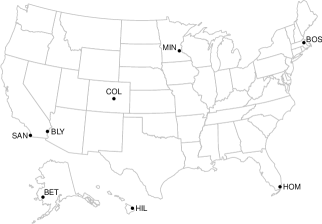
Figure 1: The eight locations from the GSOD database that are studied.

The selected stations across the U.S.  exhibit different seasonal patterns of SAT, as shown in boxplots in Figure 2 (arranged very roughly in geographic order). Most stations experience a slow increase of temperature at the end of winter, followed by a faster temperature decrease at the end of the summer, indicating complex seasonality patterns not captured by a single annual harmonic. Bethel in particular sees long winters and short summers. The most northern and continental locations (i.e., all cities in the top row of Figure 2 and Blythe) exhibit the largest amplitude of seasonality. Coastal stations at Hilo, San Diego, and Homestead experience relatively warm temperatures year round; the climate at Hilo is especially uniform. San Diego has distinctive seasonality during the first part of the year (January to June), showing an almost linear increase in the temperature with an inflection around June-July. Figure 2 also illustrates year-to-year variability of SAT on each day of the year. Seasonal variability is evident in the bulk of the distributions, represented by the box heights, as well as in the tails. Variability tends to be larger in winter and is particularly strong in the most northern locations such as Bethel. Lower and upper tails often exhibit different seasonal variability, which is evident in the various whisker lengths and the number of observations beyond the whiskers. In Bethel, many more observations lie outside the boxplot whiskers in the summer than in the winter. In Colorado Springs, values beyond the whiskers are more abundant and spread out in the lower tail than in the upper tail. Minneapolis and Homestead also present a lack of values beyond the whiskers in the upper tail during winter months, while Boston and Hilo show this behavior to a lesser extent in the lower tails during summer. The upper tail of San Diego sees the greatest number of observations beyond the whiskers, as well as the most significant spread in extremes. It is noteworthy that tail heaviness does not imply greater variability, as the SAT range in San Diego is the second smallest of the locations considered (larger only than that of Hilo). The observed asymmetries in tail behavior indicate a departure from Gaussianity and the need for non-standard distribution models.

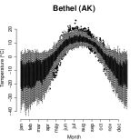
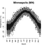
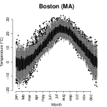
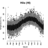
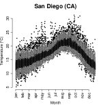
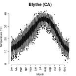
Figure 2: Boxplots of daily mean SAT at the stations considered across every day of the year for the entire studied time-period. Boxes of the boxplot are delimited by the 0.25 and 0.75 quantiles $q_{0.25}$ and $q_{0.75}$, and whiskers are $q_{0.25}-1.5\times$IQR and $q_{0.75}+1.5\times$IQR, with IQR $=q_{0.75}-q_{0.25}$ denoting the interquartile range.

3 Seasonal model for bulk and tails of temperature distribution

In this section, we detail the statistical model used to fit the temperature data described in Section 2. The proposed model relies on a univariate model for bulk and tails (Section 3.1) and is extended to a seasonal model (Section 3.2) with parameters which are estimated by maximum likelihood (Section 3.3).

3.1 Model for bulk and tails

Stein, (2020) proposed a flexible parametric model which we refer to as the bulk-and-tails (BATs) distribution. The “s” is included in the acronym to distinguish from “bulk-and-tail” models that tend to have limited flexibility in the lower tail. Consider the random variable $X$ whose cumulative distribution function (cdf) $P(X\leq x)$ is given by $T_{\nu}(H_{\theta}(x))$, where $T_{\nu}$ is the cdf of a student-$t$ random variable with $\nu$ degrees of freedom and $H_{\theta}$ is a monotone-increasing function with six parameters that control the upper and lower tails. To be precise, define $\Psi(x)=\log(1+e^{x})$ and

$$H_{\theta}(x)=\left\{1+\kappa_{1}\Psi\left(\frac{x-\phi_{1}}{\tau_{1}}\right)\right\}^{1/\kappa_{1}}-\left\{1+\kappa_{0}\Psi\left(\frac{\phi_{0}-x}{\tau_{0}}\right)\right\}^{1/\kappa_{0}}$$ (1)

where $(\phi_{i},\tau_{i},\kappa_{i})$ are the location, scale, and shape parameters of the upper $(i=1)$ and lower $(i=0)$ tails. Like in the GPD and GEV distributions, the parameters $\kappa_{i}$ control the shape of the tails, with positive values producing a heavy tailed distribution and negative values producing a thin tailed distribution with bounded support in that tail. That is, if $\kappa_{1}\geq 0$, the support $[L,U]$ has upper bound $U=\infty$, while if $\kappa_{1}<0$, then $U=\phi_{1}+\tau_{1}\Psi^{-1}(-1/\kappa_{1})$. Similarly, $L=-\infty$ if $\kappa_{0}\geq 0$ and $L=\phi_{0}-\tau_{0}\Psi^{-1}(-1/\kappa_{0})$ if $\kappa_{0}<0$. The cases $\kappa_{i}=0$ are defined by continuity. For example, when both shape parameters equal zero, $H_{\theta}$ reads

$$H_{\theta}(x)=\exp\left(\frac{x-\phi_{1}}{\tau_{1}}\right)-\exp\left(\frac{\phi_{0}-x}{\tau_{0}}\right).$$

Taking the derivative of the BATs cdf with respect to $x$, we obtain the probability distribution function (pdf) $t_{\nu}(H_{\theta}(x))H^{\prime}_{\theta}(x)$, where $t_{\nu}$ is the pdf of the student-$t$ distribution with $\nu$ degrees of freedom.

Stein, (2020) showed that this distribution can behave like any three-parameter GPD in either tail. Derivatives of the BATs pdf with respect to model parameters can be calculated analytically, aiding maximum likelihood estimation. Moreover, there is no need to numerically compute any normalizing constant when writing the density, an obstacle often handled with Markov chain Monte Carlo methods (Gelman and Meng,, 1998; Møller et al.,, 2006). Although the BATs distribution does not directly follow from any first-order limit theorems like in traditional extremes methodology, these properties produce a versatile and practical density for modeling purposes.

In this work, we attempt to model nonstationary data by allowing the scale parameters $\tau_{i}$ and location parameters $\phi_{i}$ to change with time, both seasonally and with long-term trends. In some scenarios, it may be appropriate to allow $\nu$ and $\kappa_{i}$ to also vary with time, but estimation for these parameters is already difficult when they are held constant. With a relatively simple parameterization for $\tau_{i}$ and $\phi_{i}$, we fit our model to daily SAT records at the eight U.S. cities discussed in Section 2.

3.2 Seasonal extension with long-term trend

Here we describe the seasonal model used to fit the daily SAT data to seasonal variations with a long-term trend. To capture nonstationary behaviors in SAT, namely seasonality, climate change trends, and their interaction, we introduce covariates which allow parameters of the $H_{\theta}$ function (1) to depend upon time. Reasonable choices for seasonal covariates include harmonics or a periodic spline basis; we choose the latter for more flexibility in the main seasonal term, as Figure 2 shows evidence of complex seasonal patterns. For a climate change covariate, we use the logarithm of CO₂ equivalent obtained from the PRIMAP emission time series (Gütschow et al.,, 2016) and freely available for download at https://www.pik-potsdam.de/paris-reality-check/primap-hist/. The PRIMAP time series is available on a yearly basis through 2018, and we regress PRIMAP values on the historic Mauna Loa CO₂ dataset to predict the values at 2019 and 2020. In this study, the log CO₂ equivalent serves as a proxy for climate change induced by greenhouse gases. Finally, as seasonal patterns can also be affected by the changing climate, an interaction term between seasonality and long-term trend is added, where the seasonality is modeled with annual harmonics.

Let $y$ represent the year and $d$ represent the Julian day since the first observation, modulo 365.25. Write $S_{j}(d)$ to denote the $j$^th spline basis function at day $d$ and $C(y)$ to denote the value of the log CO₂ equivalent at year $y$. Suppressing the subscripts $i=0,1$ for $\tau_{i}$ and $\phi_{i}$, we use the following parameterizations:

$$\phi(d,y) =\alpha_{0}+\sum_{j=1}^{8}\alpha_{j}S_{j}(d)+C(y)\left(\beta_{1}+\beta_{2}\cos\left(\frac{2\pi d}{365.25}\right)+\beta_{3}\sin\left(\frac{2\pi d}{365.25}\right)\right)$$

$$\log(\tau(d)) =\gamma_{0}+\sum_{j=1}^{8}\gamma_{j}S_{j}(d).$$ (2)

The long-term trend and its interaction with seasonality are only considered in the location parameters; we represent seasonality in the interaction term with circular harmonics for parsimony purposes. For simplicity, we use the same seasonal basis functions (periodic cubic splines from the R package pbs (Wang,, 2013)) for the location and scale parameters. We fix the number of seasonal basis functions at eight. Using fewer basis functions at cities with more complicated seasonal temperature variations presented problems with the optimization convergence and also a worsened fit based on model diagnostics. We found that the choices made here provided a good overall compromise between capturing the nuances of the seasonal distributions at some sites and limiting the total number of parameters for reasons of computational stability and controlling model complexity.

3.3 Maximum likelihood estimation and its uncertainty

Suppose there are independent observations $x_{1},\dots,x_{m}$ of temperature at a location. The corresponding likelihood is

$$\prod_{i=1}^{m}t_{\nu}(H_{\theta}(x_{i}))H_{\theta}^{\prime}(x_{i})$$ (3)

where $H_{\theta}$ is defined as in (1) and $t_{\nu}$ is the student-$t$ pdf with $\nu$ degrees of freedom. Note that the likelihood (3) does not explicitly include the temporal dependence between daily observations, although the uncertainty quantification described in Section 3.3 does take this dependence into consideration. Ignoring the temporal dependence does not bias point estimates of marginal distributions of individual days (Varin et al.,, 2011). In total, there are 45 parameters which are estimated via maximum likelihood: 13 parameters each for the upper and lower locations, 8 parameters each for the upper and lower scales, two shape parameters, and the degrees of freedom $\nu$. We enforced two constraints $\kappa_{i}/\nu>-0.5$ so that the likelihood is twice-differentiable at its endpoints when $\kappa_{i}$ is negative. Optimization was performed in Julia with the IPOPT solver (Biegler and Zavala,, 2009) and automatic differentiation from ForwardDiff.jl (Revels et al.,, 2016) to efficiently obtain the gradient and Hessian. For our initial guess, $\nu$ was set to 10, and all trend-related parameters and shape parameters were initially set to zero. Initial seasonal coefficients for the location parameters were obtained from linear regression. Coefficients for the log scale parameters were initially set to zero, except for the intercept term, which was profiled over with a small grid of values.

Obtaining uncertainties of estimated parameters is not straightforward. We perform uncertainty quantification with a bootstrapping procedure accounting for temporal dependence. Using stratified block bootstrap resamples, it is possible to obtain confidence intervals for any desired function of the parameters with the percentile bootstrap method (Efron and Tibshirani,, 1993). Although classical bootstrapping operates under the assumption of independent and identically distributed data, the block bootstrap is commonly used in the setting of temporal dependence (Lahiri,, 2003). Under the assumption that sub-annual temporal dependence is stronger than interannual dependence, selecting a block size of a year is natural choice, and we resample years based on a decadal stratification to preserve aspects of climate change seen over the observation period. That is, to create a bootstrapped dataset, we sample years (with replacement) from each decade, preserving the number of years in each decade from the original dataset. Maximum likelihood estimation is performed on each bootstrapped dataset, and the desired functions of parameters (e.g., quantiles, changes in quantiles over years, or parameters themselves) are computed for each fit. After ordering the bootstrapped quantities of interest from smallest to largest, pointwise 95% confidence intervals are obtained as the 2.5 and 97.5 percentiles of the ordered values. Bootstrap parameter estimates were obtained using the local optima from the fit on the full dataset as the initial guess. Example confidence intervals from 200 bootstrap samples are shown later in Figure 6 in Section 4.3 and in Table 4 in Appendix B. We emphasize that these uncertainty estimates are computed for the daily marginal distribution of SAT.

4 Results on changing daily mean temperature distributions

In this section, we present results of the proposed model fit to daily mean SAT. Section 4.1 provides a visual evaluation of the quality of the fit models. Section 4.2 shows a quantitative comparison of the proposed model to several benchmark models. In particular, we compare with skew-normal and generalized Pareto distributions to respectively assess the bulk and each tail of the fit distribution. Finally, in Section 4.3, we highlight how the proposed model is able to capture the changing seasonal patterns due to long-term trends.

To begin, we describe the benchmark distributions which are compared to the BATs distribution. First, with less of an emphasis on the tails of the distribution, we compare to a skew-normal distribution with time-varying location, scale, and skewness parameters. The skew-normal distribution was found to provide reasonable fits for temperatures in Stein, (2021). With $\phi$ and $\Phi$ respectively denoting the pdf and cdf of a standard normal random variable, the skew-normal pdf is

$$f(x)=\frac{2}{\sigma}\phi\left(\frac{x-\mu}{\sigma}\right)\Phi\left(\alpha\left(\frac{x-\mu}{\sigma}\right)\right)$$ (4)

where $\alpha$ is a skewness parameter, $\mu$ is a location parameter, and $\sigma>0$ is a scale parameter. We use the same spline-basis parameterization for the location and scale parameters as in (2) and also let the skewness vary in time using the same parameterization as the location parameter but without a climate-change covariate. Maximum likelihood estimation for the skew-normal model is performed in Julia.

To focus on the tails of the distribution, we compare with nonstationary GPD models. The GPD pdf is

$$f(x)=\frac{1}{\sigma}\left(1+\frac{\xi(x-\mu)}{\sigma}\right)^{-1-1/\xi}$$ (5)

where $\mu$ is a user-specified threshold, $\xi$ is a shape parameter, and $\sigma>0$ is a location parameter. If the shape parameter is negative, the tail is bounded; if the shape is nonnegative, the tail is unbounded. Specifically, the GPD support is $[\mu,U]$ where $U=\mu-\sigma/\xi$ if $\xi<0$ and $U=\infty$ if $\xi\geq 0.$ We construct the GPD threshold $\mu$ as a quantile regression at the $p_{\mu}=0.95$ quantile, using eight periodic spline basis functions as covariates. When considering the lower tail, we can multiply the data by $-1$ and work in the typical peaks-over-threshold setting. For GPD parameters, we consider a constant shape parameter and a temporal scale parameter whose logarithm varies in time like the location parameter in (2). All GPD models were fit by maximum likelihood with the R package extRemes (Gilleland and Katz,, 2016).

4.1 Seasonal quantile evaluation

Given the model parameter estimates, it is possible to express the distribution of daily mean SAT at any day and year, provided that the log CO₂ equivalent is available for that year. First, in Figure 3, we examine estimated quantiles during the year 2020. Quantiles from the BATs model are shown for values 0.001, 0.01, 0.1 (blue), 0.25, 0.5, 0.75 (green), and 0.9, 0.99, 0.999 (red). The black lines in each panel are observed daily maximum, minimum, and medians taken across each day of the year over all years. These maximum and minimum values serve as a proxy for upper and lower tail descriptions which would require a large amount of data to quantify precisely. We also emphasize that these maximum and minimum values are taken from the entire time series, unlike the BATs curves that are shown for the year 2020. Overall, the fitted BATs model provides a very flexible representation across the year for the bulk and both tails of the distributions, capturing: a) larger spread in both tails and sometimes in the interquartile range during winter (e.g., Colorado Springs and Homestead); b) different spread in the lower and upper tails (e.g., San Diego); c) different seasonality patterns in each tail and in the interquartile range, such as in Bethel, where the upper and lower tails exhibit significantly different seasonal patterns; d) and asymmetric seasonal patterns across the year for the eight stations where the temperature increase at the end of the winter is slower than the decrease in early fall. Quantile regression can be used to study quantiles and tail behaviors in similar fashion to Figure 3, but this approach typically involves separate analyses of the desired quantiles and comes with the possibility of producing crossing quantile curves. To avoid crossing quantiles in quantile regression, practitioners will need to turn to specialized methods (He,, 1997; Chernozhukov et al.,, 2010; Cannon,, 2018). The use of the BATs model for the entire distribution eliminates the risk of crossing quantiles.

An interesting point in Figure 3 is the large spike in January in Hilo, which corresponds to heavy rainfall and flash flooding on January 12, 2020. In terms of the BATs model, this event corresponds to the $1-(8\times 10^{-6})$ quantile, which is extremely far in the estimated tail of the distribution given the approximately 50-year duration of the Hilo data. After refitting with this value removed, the January 12 value unsurprisingly lies even further in the tail at the $1-(2\times 10^{-7})$ quantile, and the upper tail behavior $\kappa_{1}/\nu$ (see Table 4) changes from $-0.008$ to $-0.05$. While this example illustrates that a single outlying observation can have a drastic impact on tail behavior, it is noteworthy that the BATs lower tail behavior $\kappa_{0}/\nu$ is unaffected by the January 12 2020 observation and remains around $-0.05$ even after removal. Overall, the estimates appear to provide good fits to the seasonal evolution of SAT in the different locations considered.

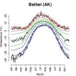
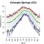
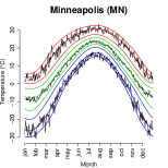
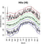
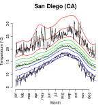
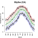
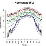
Figure 3: BATs quantile estimates for the year 2020: 0.001, 0.01, 0.1 (blue), 0.25, 0.5, 0.75 (green), and 0.9, 0.99, 0.999 (red). Black lines show the minimum/median/maximum observation for that day of year, taken over all years.

To further explore the distributions across the year, we plot individual estimated monthly densities for the first day of each of January, April, July, and October (all in 2020) from parametric models (BATs and skew-normal) along with empirical kernel density estimates (KDE) in Figure 4. Seasonal BATs and skew-normal curves are shown for the year 2020, while the KDE curves come from a Gaussian kernel density estimate using observations from a fifteen-day window over all available years. The three density curves at each location seem to largely agree with each other for all seasons and locations, but there are some notable differences. For example, in the winter and spring at Bethel, the KDE suggests a multimodal density which cannot be captured by the skew-normal estimate. In contrast, the BATs distribution has the ability to model bimodal distributions (as shown in Stein, (2020)). The presence of pronounced shoulders to the distributions which the BATs distribution can model but the skew-normal cannot is also found in the winters of Minneapolis and Homestead. These results suggest that the seasonal BATs model can capture daily mean temperature distributions more reliably than a skew-normal distribution and provide flexible densities matching observed ones. A more quantitative comparison of the skew-normal and BATs models is continued in the next section, along with a closer examination of tail properties.

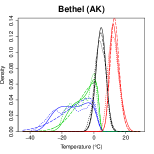
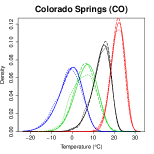
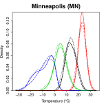
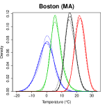
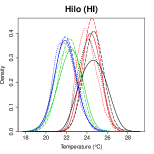
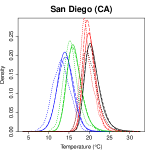
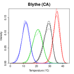
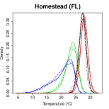
Figure 4: Density estimates for SAT distributions from the seasonal BATs model (solid), skew-normal model (long dash), and a kernel density estimate (short dash). Blue, green, red, and black curves correspond to the first day of January, April, July, and October, respectively. Parametric curves are for 2020, while the KDE curves are for the whole record.

4.2 Cross-validation comparison

We further compare our methodology to two relevant models through a quantitative analysis. To compare entire distributions, we calculate the cross-validated continuous ranked probability score (CRPS) (Gneiting and Raftery,, 2007) of the BATs and skew-normal models over the entire year and for each of the four seasons individually. CRPS is typically used in the evaluation of probabilistic forecasts as a tool to assess calibration (statistical consistency between forecast and verification data) and sharpness (dispersion of the distribution to be evaluated). By definition, CRPS values are nonnegative, and smaller values indicate a better match. The CRPS between a single observation $x$ and cdf $F$ is defined as

$$CRPS(F,x)=\int_{-\infty}^{\infty}(F(y)-\mathbf{1}[y\geq x])^{2}\;dy.$$ (6)

The CRPS is typically reported as the average of instantaneous CRPS as in (6) over a set of observations. Scores here are calculated in a cross-validation procedure where folds are obtained from blocks of four or five (consecutive) years, leading to between 10 and 20 folds depending upon the station. A scaled version of the average difference (BATs minus skew-normal) for CRPS values within a given fold is shown as a percentage in Table 1. In all cities, the CRPS difference value is negative, indicating that the BATs model fits better over the whole year, but there are some combinations of seasons and cities where the skew-normal performs better. The most noticeable improvement provided by BATs is seen in Bethel, particularly during the wintertime, consistent with the visual evidence of skew-normal misfitting the winter months shown in Figure 4.

	BET (AK)	BLY (CA)	BOS (MA)	COL (CO)	HIL (HI)	HOM (FL)	MIN (MN)	SAN (CA)
Year	-0.93	-0.14	-0.10	-0.10	-0.23	-0.18	-0.01	-0.44
DJF	-3.05	-0.27	-0.05	-0.07	-0.13	-0.12	-0.18	-0.22
MAM	-0.56	0.09	-0.10	-0.11	-0.05	-0.05	-0.08	-0.70
JJA	0.02	-0.48	-0.15	-0.21	-0.24	-0.12	0.08	-0.42
SON	-0.17	0.09	-0.10	0.01	-0.49	-0.39	0.12	-0.40

Table 1: Cross-validated CRPS comparison between the entire distribution for BATs and skew-normal. Table values equal $100\sum_{k=1}^{K}\texttt{mean}(\texttt{BATs}(k)-\texttt{Skew}(k))/\sum_{k=1}^{K}\texttt{mean}(\texttt{BATs}(k))$ where $k$ is a cross-validation fold. Negative values indicate better performance in the BATs fit. Results are tabulated for the entire year (‘Year’ row) and by season (DJF: December-January-February, MAM: March-April-May, JJA: June-July-August, SON: September-October-November).

To compare the GPD and the non-thresholded models (BATs and skew-normal), we use a variant of the CRPS. A direct CRPS comparison is not sensible because the GPD only fits a single tail of a distribution. One option to deal with this is to change the cdf in the CRPS definition (6) to the cdf conditional on being larger than the threshold. Conditioning puts the cdf of the BATs model on the same range, $[0,1]$, as the GPD model when looking above the threshold. However, this approach does not take into account the model’s ability to estimate the probability of being larger than the chosen threshold. Instead, we consider a new random variable

$$Z=\begin{cases}\mu&X\leq\mu\\ X&X>\mu,\end{cases}$$

which is censored to equal the threshold when an observation falls below the threshold. For the BATs and skew-normal models, which fit the entire temperature distribution, this censored cdf equals

$$F_{Z}(z)=\begin{cases}0&z<\mu\\ F_{X}(z)&z\geq\mu,\end{cases}$$

and for the GPD models, the censored cdf equals

$$F_{Z}(z)=\begin{cases}0&z<\mu\\ p_{\mu}+(1-p_{\mu})F_{X}(z)&z\geq\mu.\end{cases}$$

As indicated by the common notation, the censoring value $\mu$ and the GPD threshold $\mu$ are identical, but in theory they could be different. Here, $p_{\mu}=0.95$ corresponds to the quantile regression level that creates the threshold $\mu$.

To assess only tail behavior, we consider a weighted CRPS (Gneiting and Ranjan,, 2011; Taillardat et al.,, 2019) where the weight function in the integral equals one if the observation lies in the tail and zero otherwise. To be precise, the indicator-weighted score expresses as

$$wCRPS(F,x;q)=\int_{-\infty}^{\infty}(F(y)-\mathbf{1}[y\geq x])^{2}\mathbf{1}[y\geq q]\;dy$$

where $F$ is a censored cdf described above. The role of $q$ is to examine behavior of the distribution far in the tail by ignoring values smaller than $q$. Both the GPD threshold $\mu$ and the wCRPS threshold $q$ are obtained from a cross-validated quantile regression with eight periodic splines as covariates, with $\mu$ taken as the $p_{\mu}=0.95$ quantile and $q$ as the $p_{q}$ quantile, where $p_{q}\geq 0.95$. A similar procedure can be conducted to assess the lower tails of the distributions. Results from this comparison are shown in Table 2. For the most part, the BATs model and skew-normal appear to provide a slightly better fit than the GPD in this tail analysis. In Bethel, the skew-normal distribution fits the lower tail poorly, due primarily to its inability to reproduce behavior in DJF, as seen earlier in Figure 4 and Table 1. Besides the lower tail in Bethel, the BATs model and skew-normal are relatively comparable with a slight advantage to BATs. Boxplots for Colorado Springs in Figure 2 showed asymmetric behavior in the upper and lower tails, with the lack of observations beyond the upper boxplot whiskers indicating a non-Gaussian upper tail. Accordingly, the BATs and skew-normal wCRPS values in the lower tail are quite similar, yet the BATs model provides a better fit in the upper tail. In cases where the performance of BATs is particularly poor—namely, the lower tails at Blythe and Homestead—the trouble largely comes from misfit in the first cross validation fold, where fitting was done on the hold-out data which did not include initial observation years due to the configuration of the cross validation folds. The temperature records at these two locations had significant gaps after their earliest years, with Homestead missing over a decade, and Blythe missing over 30 years (see Appendix A).

	BET (AK)		BLY (CA)		BOS (MA)		COL (CO)		HIL (HI)		HOM (FL)		MIN (MN)		SAN (CA)
$p_{q}$	BATs	Skew	BATs	Skew	BATs	Skew	BATs	Skew	BATs	Skew	BATs	Skew	BATs	Skew	BATs	Skew
0.95	-0.53	-0.42	-0.51	-0.87	-0.13	-0.03	-0.46	-0.30	-4.08	-2.89	-2.41	-2.38	-0.28	-0.25	-1.20	-1.12
0.99	-0.17	-0.19	-0.71	-1.05	-0.10	0.03	-0.35	0.10	-2.06	-1.12	-2.26	-2.17	-0.09	0.00	-0.04	-0.04
0.995	-0.13	-0.17	-0.84	-1.19	-0.06	0.06	-0.36	0.18	-1.28	-0.63	-2.06	-1.89	-0.09	-0.01	0.18	0.00
0.05	-0.35	3.34	0.27	-0.27	-0.13	-0.06	-0.23	-0.21	-0.81	-0.46	-0.24	-0.30	-0.37	0.15	-1.50	-0.10
0.01	-0.06	13.38	0.91	-0.26	-0.05	0.02	-0.09	-0.09	-0.50	0.03	0.18	-0.04	-0.30	0.90	-0.82	0.15
0.005	-0.09	20.44	0.94	-0.37	-0.06	0.00	-0.06	-0.06	-0.42	0.07	0.30	0.06	-0.25	1.18	-0.45	0.13

Table 2: Cross-validated wCRPS comparison of the tail behavior beyond quantile $p_{q}$. Estimates of $\mu$ (GPD threshold where observations are censored; corresponds to $p_{\mu}=0.95$ quantile (upper tail) or $p_{\mu}=0.05$ quantile (lower tail)) and $q$ (wCRPS threshold; corresponds to $p_{q}$ quantile in left column) are obtained from cross-validated quantile regressions with eight periodic splines as covariates. Table values equal $100\sum_{k=1}^{K}\texttt{mean}(\texttt{BATs}(k)-\texttt{GPD}(k))/\sum_{k=1}^{K}\texttt{mean}(\texttt{GPD}(k))$ and $100\sum_{k=1}^{K}\texttt{mean}(\texttt{Skew}(k)-\texttt{GPD}(k))/\sum_{k=1}^{K}\texttt{mean}(\texttt{GPD}(k))$ where $k$ is a cross-validation fold. Negative values indicate better performance than the GPD fit.

4.3 Changing distributions over the years

We conclude our analysis by illustrating the ability of the proposed nonstationary BATs model to capture changes in SAT distributions and their seasonal patterns between years in a nonstationary climate. Our model explicitly accounts for a proxy of climate change through the log CO₂ equivalent incorporated in the model parameters and through the interaction between seasonality and this long-term trend. First, in Figure 5, we show how estimated seasonal quantiles from the seasonal BATs model fits evolve over the period of the observational record. Specifically, the graphs use gradations of shading from grey to black to show time evolution of the differences of the estimated 0.001, 0.1, 0.5, 0.9, and 0.999 yearly quantiles from the 0.5 quantile at the starting year. Most combinations of quantiles and stations show a warming trend (the curves become darker with increasing time). However, the details of this trend vary substantially across locations, quantile levels, and time of the year. Bethel displays substantial warming, particularly in its lower quantiles at winter months. Spring and summer months in San Diego also experience a prominent increase in the 0.999 quantile. The long-term trend and its interaction with seasonal patterns can capture evolving seasonal patterns. Changes in seasonality over the years exhibit very different patterns depending upon station location and the quantile level considered. For instance, Hilo has the largest increases in median and hot temperatures over late summer and early fall, whereas cold quantiles at Bethel warm the most during winter. A notable departure from warming is seen at Hilo, Blythe, and Colorado Springs, where the 0.001 quantile shows a cooling trend in August through December. Many cold quantiles exhibit a less pronounced seasonality in the recent years compared with past years. In particular, the seasonality of the winter cold quantiles at warmer cities flattens over time; this phenomenon is less prominent in the warm quantiles.

Figure 5: Changes of SAT quantiles from the seasonal BATs model from the beginning of the observation period (light) to the end (dark). Curves are the 0.001, 0.1, 0.5, 0.9, and 0.999 quantiles minus the 0.5 quantile at the earliest year. To emphasize differences in magnitude between stations, all subplots have the same vertical axis.

Figure 6 provides uncertainty estimates for the changes in the 0.001 and 0.999 quantiles between the first and last years of the studied period. These results are obtained from the stratified block bootstrap procedure accounting for temporal dependence discussed in Section 3.3. Note that, in general, the uncertainty bounds are not symmetric around the estimated quantile change. In particular, San Diego exhibits a very large uncertainty associated with change in 0.999 quantile from April to June, consistent with the high variability in the upper tail observed in Figures 2 and 3 at that time of the year. Table 4 shows that the BATs model in San Diego favors a heavy upper tail, and the confidence interval for the shape parameter of the upper GPD tail also includes positive values, indicating that a heavy tail is a possibility. Typical shape parameter estimates for temperature distributions range from $-0.3$ to 0 or at times are slightly positive (Nogaj et al.,, 2006; Gilleland and Katz,, 2006; Bommier,, 2014). Indeed, Figure 6 and confidence intervals from Table 4 suggest that the BATs estimate of the upper tail at San Diego may be too heavy. This large upper tail uncertainty in San Diego must be interpreted with caution, but overall, the block bootstrap helps us quantify uncertainty without neglecting temporal dependence or climate change.

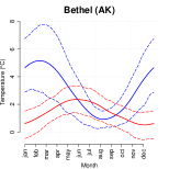
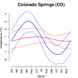
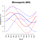
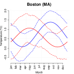
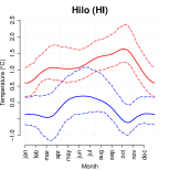
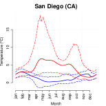
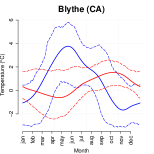
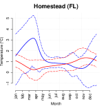
Figure 6: Bootstrap uncertainty estimates for the change in 0.001 (blue) and 0.999 (red) SAT quantiles from the starting observation year to 2020. Solid line represents the estimated quantile change, and dashed lines represent pointwise 95% bootstrap confidence intervals.

Finally, we consider the yearly evolution of quantile differences across the study period (Figure 7), which enables us to quantify changes in the spread of bulk and tails of the distribution. Specifically, we examine the interquartile range and quantile differences in the tails to assess how the bulk spread and tail spreads change over time. For comparison with the BATs model fits, quantile estimates are also obtained from a quantile regression whose covariates are eight periodic splines to quantify seasonal patterns, a long-term trend to quantify climate change, and an interaction term for long-term change in seasonal patterns (i.e., same covariates as the location parameter in (2)). We observe a strong spatial variability in the behavior of quantile spreads. In general, the width of the bulk of the distribution decreases over time, with the IQR decreasing over time in most places (e.g., Bethel) but increasing elsewhere (e.g., Hilo). Quantile differences in both the near (orange and purple) and far (red and blue) tails experience different rates of changes for cold and warm temperature. Huang et al., (2016) and Rhines et al., (2017), respectively in climate projections and historical reanalysis, reported a decrease in variability of winter temperature in most North American regions. The far warm tails (red) often show a stretching trend, whereas the near cold tails (purple) tend to contract. For most locations considered, the far tail spreads (red and blue) are smaller than the near tail spreads (orange and purple), with some few exceptions. In Colorado Springs and Homestead, both lower tail spreads are larger than the upper tail spreads. In San Diego, both upper tail spreads are larger than the lower tail spreads, and the far upper tail spread has changed at a pace that rivals the interquartile range. At Hilo, all measures of spread appear to be increasing over time. For the most part, results from BATs and quantile regression agree with one another in capturing these aspects of SAT. The largest discrepancy is in Blythe, where the BATs model lacks the increase in far lower tail spread and decrease in far upper tail spread found in results for the quantile regression. This difference seems to result from the many years of missing data at Blythe, as a stationary quantile regression for each decade (shown with horizontal lines) does not exhibit this crossing of far upper and lower tail spreads. Other stations also display a general characteristic of “flatness” in the BATs results when compared to the corresponding estimates from quantile regression. Allowing other parameters in the BATs model to depend upon log CO₂ may help capture more subtle year-to-year changes in distribution.

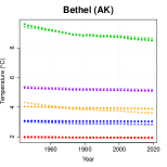
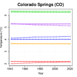
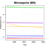
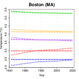
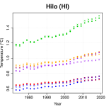
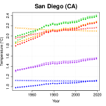
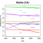
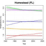
Figure 7: Average differences between quantiles for each year based on the BATs model ($\mathtt{o}$) and quantile regression ($\mathtt{x}$). Only every other year is shown. Red is $q_{0.99}-q_{0.95}$, orange is $q_{0.95}-q_{0.75}$, green is $q_{0.75}-q_{0.25}$, purple is $q_{0.25}-q_{0.05}$, and blue is $q_{0.05}-q_{0.01}$. Due to missing data at Blythe, we add lines which show stationary quantile regressions for each decade of data.

5 Discussion and Conclusions

In this paper, we have applied the seasonal bulk-and-tails (BATs) model with a long-term trend to daily mean surface air temperature data from eight cities in the United States. The model has demonstrated its ability to capture different seasonality and climate change patterns as well as different behaviors in the upper and lower tails. A cross-validation comparison shows superior fit of the BATs distribution to the skew-normal distribution on the entire distribution at all cities and to the generalized Pareto distribution in both tails at many cities.

For practitioners, this model offers a great flexibility with a closed-form density that is relatively easy to work with. Only a few statistical models proposed in extremes literature possess a density describing the bulk and both tails (Naveau et al.,, 2016; Tencaliec et al.,, 2020; Stein,, 2020, 2021). Extreme value analysis is still traditionally performed with block-maxima or peak-over-threshold techniques, which limits analysis to a tail at a time and avoids an all-encompassing model that describes the entire distribution (Coles,, 2001). The proposed framework also allows parameters in the BATs distribution to change over time, both seasonally and long-term. A stratified block bootstrap procedure was conducted for uncertainty quantification.

Of the seven parameters in the standard BATs model, we have taken the shape parameters $\kappa_{0}$ and $\kappa_{1}$ and the smoothness $\nu$ to be constant over time. This choice was made due to the difficulty of estimating the shape and smoothness even when these parameters are constant. To capture long-term variation of the nonstationary parameters, we included an annual log CO₂ equivalent covariate in the location parameters. Other parameters could depend upon this covariate, particularly the scale parameters, which would reflect a long-term change in the temperature variability, or the shape parameters, which would reflect long-term changes in tail behavior. Figure 7 indicates that it may be worth allowing other parameters to depend on the long-term trend and its seasonal interaction. Although the logarithm of CO₂ equivalent serves as a proxy for climate change induced by greenhouse gases, it is important to note that not all long-term changes in this paper are due to global-scale anthropogenic climate change. Some sites may be affected by localized changes, particularly the larger cities and those with measurements taken at airports.

The proposed model provides a flexible statistical tool to examine the bulk and tails of distributions changing over time. We have quantified how different parts of the SAT distribution (i.e., different quantiles) exhibit different seasonal and long-term changes at cities representative of different geographies and local climates. Hot and cold quantiles tend to experience larger long-term changes than median quantiles and also present different seasonal patterns. In particular, studied locations with warmer climates experience the most warming for hot quantiles in summer, and locations with colder climate experience the most warming for cold quantiles in winter.

Finally, the proposed model is fit to observations while neglecting spatial and temporal dependence. Modeling multidimensional extremes (as would be needed to explicitly account for spatial and/or temporal dependence) is an on-going challenge for the community (Huser and Wadsworth,, 2020), where various techniques have been proposed, relying on hierarchical models (Gaetan and Grigoletto,, 2007), copulas (Lee and Joe,, 2018; Krupskii and Genton,, 2021), and conditional modeling (Wadsworth and Tawn,, 2019; Simpson and Wadsworth,, 2021; Huang et al.,, 2021). Most of these methods ignore the bulk of the data or only focus on a single tail. Developing a bulk-and-tails model for multiple variables is a formidable task because of the wide range of behaviors that can occur in distributions for multivariate extremes (Huser and Genton,, 2016; Huser et al.,, 2017; Huser and Wadsworth,, 2019; Huang et al., 2019a, ; Davison et al.,, 2013).

Appendix A Complementary Data Information

	%	Start	Missing
BET (AK)	89	1945
BLY (CA)	86	1942	1945-1972
BOS (MA)	95	1943
COL (CO)	100	1942	1965-1972
HIL (HI)	99	1973
HOM (FL)	94	1943	1946-1955, 1971-1972, 2000-2004
MIN (MN)	100	1945	1965-1972
SAN (CA)	98	1945

Table 3: Summary description of the data. In particular, the percentage of daily mean SAT measurements taken with an average of over 20 hours of data, the starting year of measurements, and any years which are entirely missing data. End year is 2020.

Appendix B Parameter Estimates

	$\kappa_{0}/\nu$		$\kappa_{1}/\nu$		$\xi_{0}$		$\xi_{1}$
BET (AK)	0.019	(-0.031, 0.027)	-0.048	(-0.144, -0.008)	-0.234	(-0.328, -0.184)	-0.146	(-0.235, -0.130)
BLY (CA)	-0.034	(-0.068, 0.013)	-0.005	(-0.028, 0.016)	-0.222	(-0.326, -0.164)	-0.103	(-0.188, -0.049)
BOS (MA)	-0.245	(-0.327, -0.215)	-0.190	(-0.258, -0.149)	-0.188	(-0.285, -0.177)	-0.221	(-0.288, -0.177)
COL (CO)	-0.088	(-0.134, -0.023)	-0.156	(-0.268, -0.071)	-0.182	(-0.251, -0.139)	-0.165	(-0.208, -0.096)
HIL (HI)	-0.051	(-0.084, 0.008)	-0.008	(-0.036, 0.019)	-0.242	(-0.331, -0.176)	-0.093	(-0.169, -0.057)
HOM (FL)	-0.002	(-0.052, 0.033)	-0.009	(-0.047, 0.017)	-0.215	(-0.285, -0.167)	-0.104	(-0.243, -0.060)
MIN (MN)	-0.220	(-0.273, -0.157)	-0.251	(-0.300, -0.209)	-0.187	(-0.241, -0.143)	-0.235	(-0.303, -0.191)
SAN (CA)	0.003	(-0.141, 0.034)	0.119	(0.022, 0.239)	-0.122	(-0.217, -0.117)	-0.006	(-0.086, 0.013)

Table 4: Parameter estimates with 95% confidence interval. Two left columns are tail behaviors of the BATs model, and two right columns are tail behaviors of the GPD models. Confidence intervals obtained from the percentile method with 200 block bootstrap samples.

Appendix C Quantile Regression

The $\tau$^th quantile $(0<\tau<1$) of a random variable $Y$ with cdf $F$ is defined as $Q_{Y}(\tau)=\inf\{y\mid y\geq F(y)\}$. Quantile regression is used to estimate quantiles as a linear function of covariates $X$; that is, $X\beta\in\mathbb{R}^{n}$, where $X$ is a $n\times p$ matrix of covariates. Estimates of the coefficient vector are given by

$$\hat{\beta}=\operatorname*{arg\,min}\limits_{\beta\in{\mathbb{R}^{p}}}\sum_{i=1}^{n}\rho_{\tau}(y_{i}-x_{i}\beta)$$

where $x_{i}$ is the $i$^th row of $X$ and $\rho_{\tau}(y)=y(\tau-\mathbf{1}[y<0])$. All quantile regressions were fit with the R package quantreg (Koenker,, 2021).

Appendix D Kernel Density Estimate

Suppose we are interested in the KDE at day of year $d_{0}$. Let $A_{1943}=\{d_{-7},\dots,d_{7}\}$ be the window of days centered at $d_{0}$ for the first observation year, say 1943. With $A=A_{1943}\cup\dots\cup A_{2020}$, the KDE formula reads

$$K_{h}(x)=\frac{1}{|A|}\sum_{x_{i}\in A}K\left(\frac{x-x_{i}}{h}\right)$$

where $K$ is a Gaussian kernel function and $h$ is a bandwidth. Estimates were obtained from the density R command with bandwidth selected according to Sheather and Jones, (1991).

References

- Biegler and Zavala, (2009) Biegler, L. and Zavala, V. (2009). Large-scale nonlinear programming using ipopt: An integrating framework for enterprise-wide dynamic optimization. Computers & Chemical Engineering, 33:575–582.
- Bommier, (2014) Bommier, E. (2014). Peaks-Over-Threshold Modelling of Environmental Data. PhD thesis, Uppsala University.
- Bopp and Shaby, (2017) Bopp, G. P. and Shaby, B. A. (2017). An exponential–gamma mixture model for extreme Santa Ana winds. Environmetrics, 28(8):e2476.
- Busby et al., (2021) Busby, J. W., Baker, K., Bazilian, M. D., Gilbert, A. Q., Grubert, E., Rai, V., Rhodes, J. D., Shidore, S., Smith, C. A., and Webber, M. E. (2021). Cascading risks: Understanding the 2021 winter blackout in texas. Energy Research & Social Science, 77:102106.
- Cannon, (2018) Cannon, A. (2018). Non-crossing nonlinear regression quantiles by monotone composite quantile regression neural network, with application to rainfall extremes. Stochastic Environmental Research and Risk Assessment, 32.
- Carreau and Bengio, (2009) Carreau, J. and Bengio, Y. (2009). A hybrid Pareto model for asymmetric fat-tailed data: the univariate case. Extremes, 12(1):53–76.
- Cheng et al., (2014) Cheng, L., AghaKouchak, A., Gilleland, E., and Katz, R. W. (2014). Non-stationary extreme value analysis in a changing climate. Climatic change, 127(2):353–369.
- Chernozhukov et al., (2010) Chernozhukov, V., Fernández-Val, I., and Galichon, A. (2010). Quantile and probability curves without crossing. Econometrica, 78(3):1093–1125.
- Coles, (2001) Coles, S. (2001). An Introduction to Statistical Modeling of Extreme Values. Springer Series in Statistics. Springer-Verlag London, Ltd., London.
- Davison et al., (2013) Davison, A. C., Huser, R., and Thibaud, E. (2013). Geostatistics of dependent and asymptotically independent extremes. Math. Geosci., 45(5):511–529.
- Davison and Smith, (1990) Davison, A. C. and Smith, R. L. (1990). Models for exceedances over high thresholds. J. Roy. Statist. Soc. Ser. B, 52(3):393–442. With discussion and a reply by the authors.
- Eastoe and Tawn, (2009) Eastoe, E. F. and Tawn, J. A. (2009). Modelling non-stationary extremes with application to surface level ozone. Journal of the Royal Statistical Society: Series C (Applied Statistics), 58(1):25–45.
- Efron and Tibshirani, (1993) Efron, B. and Tibshirani, R. J. (1993). An introduction to the bootstrap, volume 57 of Monographs on Statistics and Applied Probability. Chapman and Hall, New York.
- Finkenstädt and Rootzén, (2003) Finkenstädt, B. and Rootzén, H. (2003). Extreme values in finance, telecommunications, and the environment. Chapman & Hall/CRC.
- Frigessi et al., (2002) Frigessi, A., Haug, O., and Rue, H. (2002). A dynamic mixture model for unsupervised tail estimation without threshold selection. Extremes, 5(3):219–235 (2003).
- Furrer and Katz, (2008) Furrer, E. M. and Katz, R. W. (2008). Improving the simulation of extreme precipitation events by stochastic weather generators. Water Resources Research, 44(12).
- Gaetan and Grigoletto, (2007) Gaetan, C. and Grigoletto, M. (2007). A hierarchical model for the analysis of spatial rainfall extremes. Journal of agricultural, biological, and environmental statistics, 12(4):434–449.
- Gelman and Meng, (1998) Gelman, A. and Meng, X.-L. (1998). Simulating normalizing constants: from importance sampling to bridge sampling to path sampling. Statist. Sci., 13(2):163–185.
- Gilleland and Katz, (2006) Gilleland, E. and Katz, R. (2006). Analyzing seasonal to interannual extreme weather and climate variability with the extremes toolkit. 18th Conference on Climate Variability and Change, 86th American Meteorological Society (AMS) Annual Meeting, 29.
- Gilleland and Katz, (2016) Gilleland, E. and Katz, R. (2016). extRemes 2.0: An Extreme Value Analysis Package in R. Journal of Statistical Software, 72(1):1–39.
- Gilleland et al., (2017) Gilleland, E., Katz, R. W., and Naveau, P. (2017). Quantifying the risk of extreme events under climate change. Chance, 30(4):30–36.
- Gneiting and Raftery, (2007) Gneiting, T. and Raftery, A. E. (2007). Strictly proper scoring rules, prediction, and estimation. Journal of the American Statistical Association, 102(477):359–378.
- Gneiting and Ranjan, (2011) Gneiting, T. and Ranjan, R. (2011). Comparing density forecasts using threshold- and quantile-weighted scoring rules. J. Bus. Econom. Statist., 29(3):411–422.
- Grotjahn et al., (2016) Grotjahn, R., Black, R., Leung, R., Wehner, M. F., Barlow, M., Bosilovich, M., Gershunov, A., Gutowski, W. J., Gyakum, J. R., Katz, R. W., et al. (2016). North American extreme temperature events and related large scale meteorological patterns: a review of statistical methods, dynamics, modeling, and trends. Climate Dynamics, 46(3):1151–1184.
- Gütschow et al., (2016) Gütschow, J., Jeffery, M., Gieseke, R., Gebel, R., Stevens, D., Krapp, M., and Rocha, M. (2016). The PRIMAP-hist national historical emissions time series. Earth System Science Data, 8(2):571–603.
- Hansen et al., (2010) Hansen, J., Ruedy, R., Sato, M., and Lo, K. (2010). Global surface temperature change. Reviews of Geophysics, 48(4).
- Haugen et al., (2018) Haugen, M. A., Stein, M. L., Moyer, E. J., and Sriver, R. L. (2018). Estimating changes in temperature distributions in a large ensemble of climate simulations using quantile regression. Journal of Climate, 31(20):8573–8588.
- He, (1997) He, X. (1997). Quantile curves without crossing. The American Statistician, 51(2):186–192.
- (29) Huang, W. K., Cooley, D. S., Ebert-Uphoff, I., Chen, C., and Chatterjee, S. (2019a). New exploratory tools for extremal dependence: networks and annual extremal networks. Journal of Agricultural, Biological and Environmental Statistics, 24(3):484–501.
- Huang et al., (2021) Huang, W. K., Monahan, A. H., and Zwiers, F. (2021). Estimating concurrent climate extremes: A conditional approach. Weather and Climate Extremes, 33:100332.
- (31) Huang, W. K., Nychka, D. W., and Zhang, H. (2019b). Estimating precipitation extremes using the log-histospline. Environmetrics, 30(4):e2543.
- Huang et al., (2016) Huang, W. K., Stein, M. L., McInerney, D. J., Sun, S., and Moyer, E. J. (2016). Estimating changes in temperature extremes from millennial-scale climate simulations using generalized extreme value (GEV) distributions. Advances in Statistical Climatology, Meteorology and Oceanography, 2(1):79–103.
- Huser and Genton, (2016) Huser, R. and Genton, M. G. (2016). Non-stationary dependence structures for spatial extremes. J. Agric. Biol. Environ. Stat., 21(3):470–491.
- Huser et al., (2017) Huser, R., Opitz, T., and Thibaud, E. (2017). Bridging asymptotic independence and dependence in spatial extremes using Gaussian scale mixtures. Spat. Stat., 21(part A):166–186.
- Huser and Wadsworth, (2019) Huser, R. and Wadsworth, J. L. (2019). Modeling spatial processes with unknown extremal dependence class. J. Amer. Statist. Assoc., 114(525):434–444.
- Huser and Wadsworth, (2020) Huser, R. and Wadsworth, J. L. (2020). Advances in statistical modeling of spatial extremes. Wiley Interdisciplinary Reviews: Computational Statistics, page e1537.
- Huybers et al., (2014) Huybers, P., McKinnon, K. A., Rhines, A., and Tingley, M. (2014). US daily temperatures: The meaning of extremes in the context of nonnormality. Journal of Climate, 27(19):7368–7384.
- IPCC, (2021) IPCC (2021). Climate Change 2021: The Physical Science Basis. Contribution of Working Group I to the Sixth Assessment Report of the Intergovernmental Panel on Climate Change. Cambridge University Press. In Press.
- Katz and Brown, (1992) Katz, R. W. and Brown, B. G. (1992). Extreme events in a changing climate: variability is more important than averages. Climatic change, 21(3):289–302.
- Koenker, (2021) Koenker, R. (2021). quantreg: Quantile Regression. R package version 5.85.
- Krupskii and Genton, (2021) Krupskii, P. and Genton, M. G. (2021). Conditional normal extreme-value copulas. Extremes, pages 1–29.
- Lahiri, (2003) Lahiri, S. N. (2003). Resampling methods for dependent data. Springer Series in Statistics. Springer-Verlag, New York.
- Lee and Joe, (2018) Lee, D. and Joe, H. (2018). Multivariate extreme value copulas with factor and tree dependence structures. Extremes, 21(1):147–176.
- Legates and Willmott, (1990) Legates, D. R. and Willmott, C. J. (1990). Mean seasonal and spatial variability in global surface air temperature. Theoretical and applied climatology, 41(1):11–21.
- McKinnon et al., (2016) McKinnon, K. A., Rhines, A., Tingley, M. P., and Huybers, P. (2016). The changing shape of northern hemisphere summer temperature distributions. Journal of Geophysical Research: Atmospheres, 121(15):8849–8868.
- McKinnon et al., (2013) McKinnon, K. A., Stine, A. R., and Huybers, P. (2013). The spatial structure of the annual cycle in surface temperature: Amplitude, phase, and lagrangian history. Journal of Climate, 26(20):7852–7862.
- Meehl et al., (2009) Meehl, G. A., Tebaldi, C., Walton, G., Easterling, D., and McDaniel, L. (2009). Relative increase of record high maximum temperatures compared to record low minimum temperatures in the US. Geophysical Research Letters, 36(23).
- Mentaschi et al., (2016) Mentaschi, L., Vousdoukas, M., Voukouvalas, E., Sartini, L., Feyen, L., Besio, G., and Alfieri, L. (2016). The transformed-stationary approach: a generic and simplified methodology for non-stationary extreme value analysis. Hydrology and Earth System Sciences, 20(9):3527–3547.
- Møller et al., (2006) Møller, J., Pettitt, A. N., Reeves, R., and Berthelsen, K. K. (2006). An efficient Markov chain Monte Carlo method for distributions with intractable normalising constants. Biometrika, 93(2):451–458.
- Naveau et al., (2016) Naveau, P., Huser, R., Ribereau, P., and Hannart, A. (2016). Modeling jointly low, moderate, and heavy rainfall intensities without a threshold selection. Water Resources Research, 52(4):2753–2769.
- NCEI, (2020) NCEI (2020). Global Surface Summary of Day (GSOD), National Centers for Environmental Information, National Oceanic and Atmospheric Administration, U.S. Department of Commerce. https://www7.ncdc.noaa.gov/CDO/GSOD_DESC.txt.
- Nogaj et al., (2007) Nogaj, M., Parey, S., and Dacunha-Castelle, D. (2007). Non-stationary extreme models and a climatic application. Nonlinear Processes in Geophysics, 14(3):305–316.
- Nogaj et al., (2006) Nogaj, M., Yiou, P., Parey, S., Malek, F., and Naveau, P. (2006). Amplitude and frequency of temperature extremes over the North Atlantic region. Geophysical Research Letters, 33(10):L10801.
- Peel et al., (2007) Peel, M., Finlayson, B., and Mcmahon, T. (2007). Updated world map of the Koppen-Geiger climate classification. Hydrology and Earth System Sciences Discussions, 4.
- Philip et al., (2021) Philip, S. Y., Kew, S. F., van Oldenborgh, G. J., Yang, W., Vecchi, G. A., Anslow, F. S., Li, S., Seneviratne, S. I., Luu, L. N., Arrighi, J., Singh, R., van Aalst, M., Hauser, M., Schumacher, D. L., Marghidan, C. P., Ebi, K. L., Bonnet, R., Vautard, R., Tradowsky, J., Coumou, D., Lehner, F., Wehner, M., Rodell, C., Stull, R., Howard, R., Gillett, N., and Otto, F. E. L. (2021). Rapid attribution analysis of the extraordinary heatwave on the Pacific Coast of the US and Canada June 2021. https://www.worldweatherattribution.org/western-north-american-extreme-heat-virtually-impossible-without-human-caused-climate-change/.
- Poppick et al., (2017) Poppick, A., Moyer, E. J., and Stein, M. L. (2017). Estimating trends in the global mean temperature record. Advances in Statistical Climatology, Meteorology and Oceanography, 3(1):33–53.
- Rahmstorf and Coumou, (2011) Rahmstorf, S. and Coumou, D. (2011). Increase of extreme events in a warming world. Proceedings of the National Academy of Sciences, 108(44):17905–17909.
- Reiss and Thomas, (2007) Reiss, R.-D. and Thomas, M. (2007). Statistical analysis of extreme values with applications to insurance, finance, hydrology and other fields. Birkhäuser Verlag, Basel, third edition. With 1 CD-ROM (Windows).
- Revels et al., (2016) Revels, J., Lubin, M., and Papamarkou, T. (2016). Forward-mode automatic differentiation in julia. CoRR, abs/1607.07892.
- Rhines et al., (2017) Rhines, A., McKinnon, K. A., Tingley, M. P., and Huybers, P. (2017). Seasonally resolved distributional trends of North American temperatures show contraction of winter variability. Journal of Climate, 30(3):1139–1157.
- Robin and Ribes, (2020) Robin, Y. and Ribes, A. (2020). Nonstationary extreme value analysis for event attribution combining climate models and observations. Advances in Statistical Climatology, Meteorology and Oceanography, 6(2):205–221.
- Scarrott and MacDonald, (2012) Scarrott, C. and MacDonald, A. (2012). A review of extreme value threshold estimation and uncertainty quantification. REVSTAT, 10(1):33–60.
- Schramm et al., (2021) Schramm, P. J., Vaidyanathan, A., Radhakrishnan, L., Gates, A., Hartnett, K., and Breysse, P. (2021). Heat-Related Emergency Department Visits During the Northwestern Heat Wave.
- Semenov, (2008) Semenov, M. (2008). Simulation of extreme weather events by a stochastic weather generator. Climate Research - CLIMATE RES, 35:203–212.
- Seneviratne et al., (2021) Seneviratne, S. I., Zhang, X., Adnan, M., Badi, W., Dereczynski, C., Luca, A. D., Ghosh, S., Iskandar, I., Kossin, J., Lewis, S., Otto, F., Pinto, I., Satoh, M., Vicente-Serrano, S. M., Wehner, M., and Zhou, B. (2021). Weather and Climate Extreme Events in a Changing Climate. In: Climate Change 2021: The Physical Science Basis. Contribution of Working Group I to the Sixth Assessment Report of the Intergovernmental Panel on Climate Change. Cambridge University Press. In Press.
- Sheather and Jones, (1991) Sheather, S. J. and Jones, M. C. (1991). A reliable data-based bandwidth selection method for kernel density estimation. J. Roy. Statist. Soc. Ser. B, 53(3):683–690.
- Simpson and Wadsworth, (2021) Simpson, E. S. and Wadsworth, J. L. (2021). Conditional modelling of spatio-temporal extremes for red sea surface temperatures. Spatial Statistics, 41:100482.
- Sparks et al., (2017) Sparks, A., Hengl, T., and Nelson, A. (2017). GSODR: Global Summary Daily Weather Data in R. The Journal of Open Source Software, 2.
- Stein, (2020) Stein, M. L. (2020). A parametric model for distributions with flexible behavior in both tails. Environmetrics.
- Stein, (2021) Stein, M. L. (2021). Parametric models for distributions when interest is in extremes with an application to daily temperature. Extremes, 24(2):293–323.
- Taillardat et al., (2019) Taillardat, M., Fougères, A.-L., Naveau, P., and de Fondeville, R. (2019). Extreme events evaluation using CRPS distributions.
- Tarleton and Katz, (1995) Tarleton, L. F. and Katz, R. W. (1995). Statistical explanation for trends in extreme summer temperatures at Phoenix, Arizona. Journal of Climate, 8(6):1704–1708.
- Tencaliec et al., (2020) Tencaliec, P., Favre, A.-C., Naveau, P., Prieur, C., and Nicolet, G. (2020). Flexible semiparametric Generalized Pareto modeling of the entire range of rainfall amount. Environmetrics, 31(2):e2582.
- Varin et al., (2011) Varin, C., Reid, N., and Firth, D. (2011). An overview of composite likelihood methods. Statist. Sinica, 21(1):5–42.
- Wadsworth and Tawn, (2019) Wadsworth, J. L. and Tawn, J. (2019). Higher-dimensional spatial extremes via single-site conditioning. arXiv preprint arXiv:1912.06560.
- Wang, (2013) Wang, S. (2013). pbs: Periodic B Splines. R package version 1.1.
- Wehner, (2020) Wehner, M. F. (2020). Characterization of long period return values of extreme daily temperature and precipitation in the CMIP6 models: Part 2, projections of future change. Weather and Climate Extremes, 30:100284.
- Yadav et al., (2021) Yadav, R., Huser, R., and Opitz, T. (2021). Spatial hierarchical modeling of threshold exceedances using rate mixtures. Environmetrics, 32(3):e2662.