Universal conductance scaling of Andreev reflections using a dissipative probe

Abstract

The Majorana search is caught up in an extensive debate about the false-positive signals from non-topological Andreev bound states (ABSs). We introduce a remedy using the dissipative probe to generate electron-boson interaction. We theoretically show that the interaction-induced renormalization leads to significantly distinct universal zero-bias conductance behaviors, i.e. distinct characteristic power-law in temperature, for different types of Andreev reflections, which shows a sharp contrast to that of a Majorana zero mode. Various specific cases have been studied, including the cases that two charges involved in an Andreev reflection process maintain/lose coherence, and the cases for multiple ABSs with or without a Majorana present. A transparent list of conductance features in each case is provided to help distinguishing the observed subgap states in experiments, which also promotes the identification of Majorana zero modes.

Introduction. Quantum tunneling Wolf (2012) has been used as a very powerful method to study quantum materials and quantum devices. However, if obtained using non-interacting probe and target, the tunneling signal is usually very sensitive to contaminants that potentially induce non-universal behaviors. As an important example, the tunneling spectroscopy signals in detecting Majorana zero modes (MZMs)  Read and Green (2000); Kitaev (2001) in semiconductor-superconductor heterostructures Lutchyn et al. (2010); Oreg et al. (2010); Lutchyn et al. (2018) should give a quantized zero-bias conductance peak Sengupta et al. (2001); Law et al. (2009); Flensberg (2010); Wimmer et al. (2011) and a robust quantized plateau by varying all relevant control parameters. However, the current experimental results Mourik et al. (2012); Deng et al. (2012); Das et al. (2012); Finck et al. (2013); Churchill et al. (2013); Deng et al. (2016); Zhang et al. (2017a); Chen et al. (2017); Suominen et al. (2017); Nichele et al. (2017); Gül et al. (2018); Vaitiekėnas et al. (2018); de Moor et al. (2018); Bommer et al. (2019); Grivnin et al. (2019); Pan et al. (2020); Zhang et al. (2021a); Song et al. (2021) are far from the ideal predictions. One of the key reasons is that such a non-interacting Majorana detection platform is easily contaminated by junction and disorder-induced Andreev bound states (ABSs) Pientka et al. (2012); Liu et al. (2012); Cole et al. (2016); Liu et al. (2017, 2018a); Cao et al. (2019); Pan and Das Sarma (2020); Sarma and Pan (2021); Pan et al. (2021) that cause non-robust signals.

As a possible remedy, interaction, known as a method to sharpen transition between different fixed points, can be introduced to classify different physics under the interaction renormalization Cardy (1996). Indeed, different physics emerges near fixed points that belong to distinct interaction-dependent universality classes. One of the simplest schemes to introduce interaction is to consider a dissipative electromagnetic environment, e.g., applying an ohmic resistance in series with the tunneling junction, and causing effective electron-boson interaction Ingold and Nazarov (1992). With ohmic dissipation, the tunneling conductance exhibits dissipation-dependent power-law scaling behaviors Ingold and Nazarov (1992). Various kinds of dissipation-influenced charge transport in mesoscopic systems have been studied both experimentally Mebrahtu et al. (2012, 2013); Jezouin et al. (2013); Anthore et al. (2018) and theoretically Matveev and Glazman (1993); Safi and Saleur (2004); Le Hur and Li (2005); Florens et al. (2007); Liu (2013); Liu et al. (2014); Zheng et al. (2014); Wölms and Flensberg (2015); Zhang et al. (2017b); Le Hur et al. (2018); Liu et al. (2020); Zhang et al. (2021b).

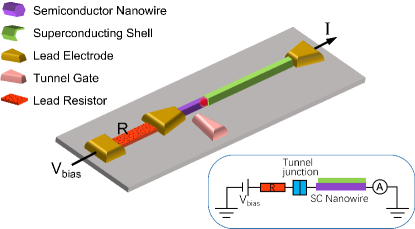
Figure 1: Illustration of the system setup. The inset is the equivalent circuit. A bias voltage $V_{\text{bias}}$ is applied on the lead.

Main results. Here, we focus on the hybrid semiconductor superconductor nanowire device for the detection of Majorana resonance. The dissipative tunneling into a MZM was proposed as a Majorana signature filter Liu (2013) by one of the authors. It is believed that junction and/or disorder-induced fermionic ABSs dominate the phase diagram of the current nanowire devices Sarma and Pan (2021); Zeng et al. (2021). Therefore, it is an interesting topic to study the dissipative interacting probe for different types of ABSs and obtain their universal scaling behaviors under renormalization to distinguish between ABSs and the real MZM. Following this motivation, we map the dissipative tunneling into ABSs to a Coulomb gas model, and find that the zero-bias conductance has special power-law dependence on temperature $T$. In addition, we find that the coherence between electron and hole after the Andreev reflection will significantly affect the power-law behaviors; and therefore, the measurement of the power-law could be applied to detect the coherence after the Andreev reflection. We show that the dissipation can cause significantly different universal behaviors according to their characteristic power law as summarized in Table 1 for different types Andreev reflections and MZM, where $r=Re^{2}/h$ is the dimensionless dissipation amplitude. Our result also potentially applies to other platforms using scanning tunneling microscope  Sun et al. (2016); Wang et al. (2018); Liu et al. (2018b); Kong et al. (2019); Machida et al. (2019), where dissipation-induced dynamical Coulomb blockade features have been observed Brun et al. (2012).

Table 1: Universal Scaling Behaviors of different circumstances.

	Majorana Liu (2013)	ABS (coherent)	ABS (incoherent)	Normal state Ingold and Nazarov (1992)
Qualitative	Enhancement	Decay	Decay	Decay
Universal scaling	$\frac{2e^{2}}{h}-G\sim T^{\frac{2-4r}{1+2r}}$	$G\sim T^{8r}$	$G\sim T^{4r}$	$G\sim T^{2r}$

Model. An illustration of the system is shown in Fig. 1. The dissipative tunneling to an ABS is achieved by tunnel coupling a lead to a nanowire. We consider the hybrid semiconductor nanowire$-$superconductor devices with finite magnetic field Lutchyn et al. (2010); Oreg et al. (2010). This type of devices are recently well-studied for the detection of MZMs. Later we also call this hybrid device the “SC nanowire”. In reality, devices of this type are easily contaminated by disorders in the junction or the nanowire bulk, and the disorder-induced trivial ABSs potentially produce false-positive signals in the standard tunneling experiments. The system is also coupled to a dissipative bath, which can be achieved by replacing part of the electrode with a thin long resistive metal strip [with resistance $R$; red in Fig. 1(a)]. The tunnel-gate controls the coupling between the lead and the SC nanowire. An equivalent circuit diagram is shown in Fig. 1(b).

The whole system includes four parts: the SC nanowire, the lead, the tunneling part, and the dissipative environment. For the SC nanowire, we focus on the case with an ABS localized at the left side of the nanowire, and its Hamiltonian can be written as $H_{\text{wire}}=\epsilon a^{\dagger}a+\text{const,}$ where $a$ is the fermionic quasiparticle operator for the ABS. Its energy is inside the superconducting gap $\epsilon<\Delta$ and can reach $\epsilon\rightarrow 0$ by adjusting experimental variables. The lead can be described by the Hamiltonian of spinful fermions with dispersion linearized close to the Fermi energy:

$$H_{\text{lead }}=v_{F}\!\sum_{\sigma=\uparrow/\downarrow}^{N}\!\int_{-\infty}^{0}\!dx\,\psi_{L,\sigma}^{\dagger}i\partial_{x}\psi_{L,\sigma}-\psi_{R,\sigma}^{\dagger}i\partial_{x}\psi_{R,\sigma},$$ (1)

where $\psi_{L,\sigma}\left(x\right)$ and $\psi_{R,\sigma}\left(x\right)$ are fermion operators for the left-moving and right-moving modes with spin $\sigma$ at point $x$ in the lead. Counting the degrees of freedom of the particle (hole) and the spin, there are a total of four conducting channels in the lead. The tunneling part of the Hamiltonian can be expressed as

$$H_{T}=\left(\psi_{\uparrow}^{\dagger}\left(0\right)\hskip 1.99997pt\psi_{\downarrow}^{\dagger}\left(0\right)\right)\left(\begin{array}[]{cc}t_{e\uparrow}&t_{h\uparrow}^{*}\\ t_{e\downarrow}^{*}&t_{h\downarrow}\end{array}\right)\left(\begin{array}[]{c}a\\ a^{\dagger}\end{array}\right)e^{-i\varphi}+h.c.,$$ (2)

where $\psi_{\sigma}(0)=\psi_{L,\sigma}(0)+\psi_{R,\sigma}(0)$. Breaking the spin rotation and time reversal symmetries, we need four independent tunneling parameters $t_{e\uparrow}$, $t_{e\downarrow}$, $t_{h\uparrow}$, $t_{h\downarrow}$ to describe an arbitrary ABS, as shown in Fig. 2(a). The operator $e^{-i\varphi}$ is conjugate to the charge fluctuation $Q$ of the junction capacitance, following $\left[\varphi,Q\right]=ie$, and thus accompanies nanowire-superconductor charge transport. It couples bilinearly to the dissipative environment represented by a set of harmonic oscillators (i.e., $\left\{q_{n},\varphi_{n}\right\}$ with oscillator frequency $\omega_{n}=1/\sqrt{L_{n}C_{n}}$) Leggett et al. (1987); Ingold and Nazarov (1992); Caldeira and Leggett (1981): $H_{\text{env}}={Q^{2}}/{2C}+\sum_{n=1}^{N}\left[{q_{n}^{2}}/{2C_{n}}+\left({\hbar}/{e^{2}}\right)^{2}\left(\varphi-\varphi_{n}\right)^{2}/{2L_{n}}\right]$, where $C_{n}$ and $L_{n}$ respectively refer to the effective capacitance and impedance of the $n$th dissipative mode.

Effective action and Coulomb gas model. Overall, the partition function of this tunnel junction coupled to the dissipative environment is

$$Z=\int\left[D\Phi_{\uparrow}\right]\left[D\Phi_{\downarrow}\right]\left[D\varphi\right]\left[Da\right]e^{-S_{\text{eff}}}e^{-S_{\text{T}}},$$ (3)

where $S_{\text{T}}$ is the action of the tunneling part $S_{\text{T}}=\int_{0}^{\beta}d\tau L_{\text{T}}$ with the tunneling Lagrangian $L_{\text{T}}$ directly obtained from Eq. (2), and $\beta$ is the temperature inverse. After a spatial integral, the effective action becomes $S^{\text{eff}}\!\!=\!\frac{1}{\beta}\sum_{\omega_{n}}\left|\omega_{n}\right|\left[\sum_{\sigma}\left|\Phi_{\sigma}\left(\omega_{n}\right)\right|^{2}+\left|\varphi\left(\omega_{n}\right)\right|^{2}/2r\right]$, with the first and the second terms in the brackets from the lead and the environment parts respectively. For later convenience, we define $r=Re^{2}/h$ as the dimensionless dissipation. $\Phi_{\sigma}\left(x\right)$ is the chiral Bosonic field from the standard Bosonization Giamarchi (2003): $\psi_{L/R,\sigma}\left(x\right)=\frac{1}{\sqrt{2\pi\alpha}}F_{\sigma}e^{-i\Phi_{\sigma}\left(\mp x\right)}$, where $\alpha$ is the short-distance cutoff and $F_{\sigma}$ is the Klein factor. In the action $S^{\text{eff}}$, the lead part is obtained by integrating out fluctuations in $\Phi_{\sigma}\left(x\right)$ away from $x=0$ Anderson et al. (1970); Kane and Fisher (1992a, b); Furusaki and Nagaosa (1993); Sup , and the environment is obtained by integrating out the environmental degree of freedom Weiss (2012).

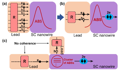
Figure 2: (a) All possible processes. (b) Leading process after RG. (c)Incoherent dissipative Andreev reflection via a cluster of ABSs.

By expending the partition function Eq. (3) in the powers of tunneling part and then integrating out the bosonic field, we can obtain the Coulomb gas representation Anderson et al. (1970); Kane and Fisher (1992a) for our model

$$Z= \sum_{\nu=\pm 1}\sum_{n}\sum_{\left\{q_{i}\right\}}\sum_{\left\{s_{i}\right\}}C_{\text{t}}\int_{0}^{\beta}d\tau_{2n}\int_{0}^{\tau_{2n}}d\tau_{2n-1}$$

$$...\int_{0}^{\tau_{3}}d\tau_{2}\int_{0}^{\tau_{2}}d\tau_{1}e^{\sum_{i>j}V_{ij}}e^{\nu\epsilon\left[\frac{\beta}{2}+\sum_{i}\left(-1\right)^{i}\tau_{i}\right]},$$ (4)

which describes a 1D plasma of logarithmically interacting charges. The interaction $V_{ij}$ has the form:

$$V_{ij}=\frac{1}{2g}\biggl{[} q_{i}q_{j}+K_{1}\left(q_{i}r_{j}+r_{i}q_{j}\right)+gs_{i}s_{j}$$

$$+K_{2}g\left(s_{i}r_{j}+r_{i}s_{j}\right)\biggr{]}\text{ln}\left(\frac{\tau_{i}-\tau_{j}}{\tau_{c}}\right),$$ (5)

where the effective interaction parameter $g=\left(1+4Re^{2}/h\right)^{-1}=(1+4r)^{-1}$, and $1/\tau_{c}$ refers to the high-energy cutoff that changes during each RG step. Three types of charges, i.e., $q_{i}$, $s_{i}$ and $r_{i}$ are involved. The first two refer to the changes in charge and spin in the lead. The last one is from the ABS state. Initially, $K_{1}=K_{2}=0$. They begin to grow in the presence of asymmetry, driving the system towards different fixed points Sup .

RG analysis and scaling behaviors. In the framework of the Coulomb gas model, the renormalization group (RG) equation at weak tunneling coupling fixed point can be obtained from integrating out the degrees of freedom between $\tau_{c}$ and $\tau_{c}+d\tau_{c}$ (a real-space RG) Sup . The resulting RG equations yield

$$\frac{dK_{1}}{d\ln\tau_{c}}= -2\tau_{c}^{2}\left[\left(\left|t_{e\uparrow}\right|^{2}-\left|t_{h\uparrow}\right|^{2}+\left|t_{e\downarrow}\right|^{2}-\left|t_{h\downarrow}\right|^{2}\right)\right.$$

$$\left.+\left(\left|t_{e\uparrow}\right|^{2}+\left|t_{h\uparrow}\right|^{2}+\left|t_{e\downarrow}\right|^{2}+\left|t_{h\downarrow}\right|^{2}\right)K_{1}\right],$$ (6a)

$$\frac{dK_{2}}{d\ln\tau_{c}}= -2\tau_{c}^{2}\left[\left(\left|t_{e\uparrow}\right|^{2}-\left|t_{h\uparrow}\right|^{2}-\left|t_{e\downarrow}\right|^{2}+\left|t_{h\downarrow}\right|^{2}\right)\right.$$

$$\left.+\left(\left|t_{e\uparrow}\right|^{2}+\left|t_{h\uparrow}\right|^{2}+\left|t_{e\downarrow}\right|^{2}+\left|t_{h\downarrow}\right|^{2}\right)K_{2}\right],$$ (6b)

$$\frac{dt_{\xi}}{d\ln\tau_{c}}= \left[1-\frac{\left(K_{1}+\delta_{\xi,1}\right)^{2}+g\left(K_{2}+\delta_{\xi,2}\right)^{2}}{4g}\right]t_{\xi},$$ (6c)

$$\frac{d\epsilon}{d\ln\tau_{c}}= \ \epsilon,$$ (6d)

where $\xi$-dependent charge pair $\left(\delta_{\xi,1},\delta_{\xi,2}\right)$ equals $\left(+1,+1\right)$, $\left(-1,-1\right)$, $\left(+1,-1\right)$, $\left(-1,+1\right)$ respectively, when $\xi$ $=e{\uparrow}$, $h{\uparrow}$, $e{\downarrow}$ and $h{\downarrow}$. For simplicity, we begin with the fine-tuned situation where $\epsilon=0$. Initially, $K_{1}=K_{2}=0$, and all tunneling operators of Eq. (2) share the same scaling dimension [i.e., the factor after the minus sign of Eq. (6c)] $1/2+r$. Following Eq. (6), the system flows to different fixed points depending on the symmetry among tunneling parameters $t_{\xi}$.

As the starting point, we look into the most generic situation and impose no requirement on tunneling parameters. Of this situation, absolute values of parameters $K_{1}$ and $K_{2}$ increase during the RG flow. Accompanying their enhancement, scaling dimension of the tunneling with the strongest amplitude begins to decrease, which in term induces an even stronger asymmetry or difference among tunnelings $\propto t_{\xi}$. To obtain a more intuitive understanding, we consider the fixed point where $t_{e\uparrow}\sim 1\gg t_{e\downarrow},t_{h\uparrow}$, $t_{h\downarrow}$, and $K_{1}=K_{2}=-1$. At this point, the leading process $\propto t_{e\uparrow}$ has a vanishing scaling dimension, and grows as if it was an energy cutoff. Consequently, at low enough temperatures, $t_{e\uparrow}\psi^{\dagger}_{\uparrow}a+h.c.$ becomes infinite, where $\psi_{\uparrow}$ completely hybridizes the impurity ABS, and at meanwhile, suppresses the other communications between the ABS and the lead. A persistent lead-superconductor transport now has to rely on coherent Andreev tunneling $t_{e\uparrow}t_{h\downarrow}\psi_{\uparrow}^{\dagger}(0)\psi_{\downarrow}^{\dagger}(0)e^{-2i\varphi}a^{\dagger}a+h.c.$. As an Andreev tunneling consists of two coherent tunnelings [Fig. 2(b)], its low-energy feature is determined by the less relevant process $\propto t_{h\downarrow}$. Following Eq. (6), this process flows $dt_{h\downarrow}/d\ln\tau_{c}=-4rt_{h\downarrow}$ when $K_{1}=K_{2}=-1$, with the scaling dimension $1+4r$. This scaling dimension indicates that at low enough temperatures, the zero-bias conductance decreases following the temperature power-law $G\propto T^{8r}$ and vanishes at zero temperature, different from the regular dissipation tunneling ($G\propto T^{2r}$ ) without superconductivity. As a reminder, the temperature power equals twice the difference between the scaling dimension and unity Kane and Fisher (1992b).

This $8r$-power-law, however, requires perfect coherent Andreev reflections. In reality, the imperfection of the superconductor-proximitized nanowire induces possible transient states with the typical lifetime $t_{\text{imp}}$. Even when two sub-processes of an Andreev tunneling are coherent, the relaxation of two involved charges, during which dissipation is produced, might lose coherence in an imperfect nanowire Inc . Indeed, we consider the Andreev tunneling operator $\mathcal{O}_{\text{AR}}=\psi^{\dagger}_{\uparrow}a\exp(-i\varphi)\psi^{\dagger}_{\downarrow}a^{\dagger}\exp(-i\varphi)+h.c.$, whose correlation in time becomes

$$\big{\langle}\mathcal{O}_{\text{AR}}(t)\mathcal{O}_{\text{AR}}(0)\big{\rangle}=\big{\langle}H^{0}_{\text{T}}(t)H^{0}_{\text{T}}(0)\big{\rangle}$$ (7)

$$\cdot \big{\langle}e^{-i\varphi(t+\delta t)}e^{-i\varphi(t+\delta t^{\prime})}e^{i\varphi(\delta t)}e^{i\varphi(\delta t^{\prime})}\big{\rangle},$$

where $H^{0}_{\text{T}}=\psi^{\dagger}_{\uparrow}a\psi^{\dagger}_{\downarrow}a^{\dagger}$ contains the lead operators, and $\delta t,\ \delta t^{\prime}\sim t_{\text{imp}}$ refer to the incoherence-induced delay in time Sup . Their amplitudes determine the leading feature of the correlation Eq. (7). Indeed, when $t\gg t_{\text{imp}}$, the delay in time becomes negligible, where the correlation of two dissipative phases $\propto t^{-8r}$. In contrast, the correlation changes to be $\propto t^{-4r}$ for relatively shorter time $t\ll t_{\text{imp}}$. The correlation of phase is then determined by the cutoff in time, i.e., the inverse of the temperature $1/T$.

Extremely, when $t_{\text{imp}}\gg 1/T$, two phases become completely uncorrelated Sup , thus reducing the suppression of conductance from dissipation by half [see Fig. 2(c)]. In this limit, Andreev reflection has the scaling dimension $1+2r$ instead, leading to the conductance power-law $G\propto T^{4r}$. As a possible extension, the coherence-dependent conductance power-law, which could potentially exist in other dissipative systems, provides us a possible tool in the detection of system coherence. In our system, incoherent power-law might also occur in relatively high-temperature systems where ABS has not been fully hybridized by the dominant lead operator. In this situation, an incoming electron might stay on the ABS for a long-enough time during which the incoming electron and the reflected hole have become incoherent.

Conductance peaks. Experimentally, two types of conductance peaks might be observed. Firstly, and the most interestingly, a Majorana resonance peak emerges when normal lead couples either to a topological MZM, or when the ABS consists of two spatially separated MZMs that decouple from each other (i.e., the quasi-MZM scenario predicted by e.g., Prada et al. (2012); Kells et al. (2012); Moore et al. (2018a, b); Vuik et al. (2019)) in case of a smooth lead-wire barrier Kells et al. (2012). These two situations are indistinguishable from local measurements, and luckily, both display non-trivial behaviors including non-Abelian statistics (see, e.g.,Vuik et al. (2019)). In our model, an accidental MZM scenario occurs when fine-tuning $|t_{e\uparrow}|^{2}-|t_{h\uparrow}|^{2}+|t_{e\downarrow}|^{2}-|t_{h\downarrow}|^{2}=0$, and $t_{e\uparrow}t_{h\downarrow}=t^{*}_{e\downarrow}t^{*}_{h\uparrow}$, where only $(a+a^{\dagger})/\sqrt{2}$ couples to the lead Majorana $(\psi_{\uparrow^{\prime}}-\psi^{\dagger}_{\uparrow^{\prime}})/\sqrt{2}$, where $\psi^{\dagger}_{\uparrow^{\prime}}$ refers to the fermion with the spin along the direction determined by relative amplitudes of $t_{e\uparrow}+t^{*}_{h\uparrow}$ and $t^{*}_{e\downarrow}+t_{h\downarrow}$ (e.g., $\uparrow^{\prime}$ points towards the $x$ direction if $t_{e\uparrow}+t^{*}_{h\uparrow}=t^{*}_{e\downarrow}+t_{h\downarrow}$). Of this scenario, two asymmetry parameters $K_{1}=K_{2}=0$ are fixed at zero, indicating the protection of the zero-bias conductance peak $2e^{2}/h$ by system symmetry at zero temperature. Specifically, as the lead-Majorana coupling has the scaling dimension $r+1/2$ initially, its dual operator at low temperatures has the scaling dimension $2/(1+2r)$, the inverse of the initial scaling. From that one arrives at the power law $2e^{2}/h-G\sim T^{\frac{2-4r}{1+2r}}$ that agrees with the result of Ref. Liu (2013), where tunneling to a real Majorana is considered.

Although theoretically any dissipation is capable of killing generic (i.e., not fine-tuned) ABS peaks at low enough energies, in real experiments ABS peaks might emerge when electron temperature is too high to witness the conductance suppression from a weak dissipation. This is especially true for a weak asymmetry among tunnelings parameters. Nevertheless, we expect the absence of universality near these ABS peaks, as they do not correspond to fixed points in a dissipative system following RG equations (6). We emphasize that the missing of universality near the ABS peak does not contradict the materials of Table. 1, where scaling behaviors are only predicted near the zero-conductance fixed point, at low-enough temperatures. For instance, we study the case where $t_{e\uparrow}=0.25$ is slightly larger than $t_{h\downarrow}$ and much larger than the other two parameters. In this situation the system conductance and its dependence on temperature are mostly determined by $t_{h\downarrow}$. In Fig. 3, we thus plot $t_{h\downarrow}$ and its scaling dimension $D(t_{h\downarrow})$ [i.e., $\left(K_{1}-1\right)^{2}/4g+\left(K_{2}+1\right)^{2}/4$ of Eq. (6c)] to indirectly investigate the conductance features. In Fig. 3(a), for a weak dissipation $r=0.1$, the conductance arrives at its peak value [where $D(t_{h\downarrow})=1$ ] when $T\approx 0.05T_{0}$, where $T_{0}$ refers to temperature at which RG starts. However, near this peak position, $D(t_{h\downarrow})$ keeps changing with temperature, indicating the absence of universality, i.e., persuasive temperature power-laws of conductance under low-enough energies. For a stronger dissipation $r=0.45$ (while fixing other parameters) shown in Fig. 3(b), the tunneling $\propto t_{h\downarrow}$ becomes irrelevant in a larger regime ($T<1.1T_{0}$), indicating a more strongly suppressed ABS tunneling. Therefore, we can see that an ABS peak is more sensitive to dissipation.

Briefly, in contrast to a Majorana zero-bias peak, ABS zero-bias peaks do not have a universal height, and in most cases do not necessarily display universality in higher temperature Sup . Indeed, following Table. 1, generic ABS conductance curves display universality only when the system flows close enough to the low temperature fixed point. However, our results suggest that a stronger dissipation (larger $r$ but smaller than $0.5$) can easily suppress the ABS peak and provide a sharp difference compared with Majorana peak.

Figure 3: Scaling dimension and amplitude (inset) of the operator $\propto t_{h\downarrow}$, when $t_{e\uparrow}$ is dominating. Temperature decreases when value of $x$-axis increases. (a) When $r=0.1$, $t_{h\downarrow}$ becomes RG irrelevant when $T\approx 0.05T_{0}$, with the peak height $\approx 0.7$. (b) When $r=0.45$, the ABS conductance arrives at its peak position much faster $T\approx 0.11T_{0}$, with a much smaller peak height $\approx 0.24$. Other parameters in (a) and (b) are the same.

Detuned ABS and multiple-ABS scenarios. In real experiment, scaling dimensions listed in Table. 1, which are among our central conclusions, should be checked carefully, as (i) the ABS energy might be finite; and (ii) multiple on-resonance ABSs might talk to the lead simultaneously, and (iii) a Majorana might become surrounded by multiple ABSs Sun et al. (2016).

As the response to the concern (i), we notice that the ABS detuning Hamiltonian $H_{\text{ABS}}=\epsilon a^{\dagger}a$ is highly RG relevant from Eq. (6d). The detuning energy should thus be considered as another possible low-energy cutoff, in addition to temperature $T$ for the zero-bias situation. Consequently, if $T\gg\epsilon$, RG flow does not see the coupling $\epsilon$, and then the conductance behavior then coincides with that when $\epsilon=0$. In the opposite limit $T\ll\epsilon$ the single-electron tunneling (e.g., $\psi_{\uparrow}^{\dagger}a$) requires to pay an extra energy, and is thus suppressed. In both limits, Andreev tunneling dominates at low temperatures, leading to the same temperature dependence as shown in Table. 1. Finally, the crossover $T\sim\epsilon$ is not within the universality class, and conductance should not follow any temperature power-law. The concern (ii), i.e., the multi-ABS scenario, can be analyzed following the g-theorem, which states that the system prefers the lower-entropy ground state Affleck and Ludwig (1991). ABSs either decouple or become fully hybridized by the lead at low enough temperatures. Of this situation, charge transport is only possible via Andreev reflection. The result is once again the same as in Table. 1.

The situation becomes most interesting if the superconductor hosts a single MZM (either topological or quasi) and one or multiple generic ABSs. At lowest energies, the system behavior is not hard to speculate following our analysis above on the multi-ABS scenario: all ABSs become decoupled or hybridized, and lead-wire charge transport relies on tunneling into the MZM. Consequently, for generic cases, we expect the same low-temperature behavior as the MZM situation of Table. 1, given low-enough temperatures. However, how the system arrives at this fixed point might depend on, e.g., the relative amplitudes of the lead-ABS and the lead-MZM couplings. Indeed, when lead-ABS coupling is stronger at high temperatures, one might expect the non-trivial transition from ABS-like to MZM-like scaling behaviors as reducing temperature.

Finally, we also notice a related experimental progress in the study of Andreev reflections using a dissipative probe in the SC nanowire devices Zhang et al. (2021c).

Acknowledgments. The work is supported by Natural Science Foundation of China (Grants No. 11974198 and No. 12004040) and Tsinghua University Initiative Scientific Research Program.

See pages 1 of DissipativeABS-SI-VF.pdf See pages 2 of DissipativeABS-SI-VF.pdf See pages 3 of DissipativeABS-SI-VF.pdf See pages 4 of DissipativeABS-SI-VF.pdf See pages 5 of DissipativeABS-SI-VF.pdf See pages 6 of DissipativeABS-SI-VF.pdf See pages 7 of DissipativeABS-SI-VF.pdf See pages 8 of DissipativeABS-SI-VF.pdf See pages 9 of DissipativeABS-SI-VF.pdf

References

- Wolf (2012) E. L. Wolf, Principles of electron tunneling spectroscopy, Vol. 152 (Oxford University Press, 2012).
- Read and Green (2000) N. Read and D. Green, Phys. Rev. B 61, 10267 (2000).
- Kitaev (2001) A. Y. Kitaev, Physics-Uspekhi 44, 131 (2001).
- Lutchyn et al. (2010) R. M. Lutchyn, J. D. Sau, and S. Das Sarma, Phys. Rev. Lett. 105, 077001 (2010).
- Oreg et al. (2010) Y. Oreg, G. Refael, and F. Von Oppen, Physical review letters 105, 177002 (2010).
- Lutchyn et al. (2018) R. M. Lutchyn, E. P. Bakkers, L. P. Kouwenhoven, P. Krogstrup, C. M. Marcus, and Y. Oreg, Nature Reviews Materials 3, 52 (2018).
- Sengupta et al. (2001) K. Sengupta, I. Žutić, H.-J. Kwon, V. M. Yakovenko, and S. Das Sarma, Phys. Rev. B 63, 144531 (2001).
- Law et al. (2009) K. T. Law, P. A. Lee, and T. K. Ng, Phys. Rev. Lett. 103, 237001 (2009).
- Flensberg (2010) K. Flensberg, Phys. Rev. B 82, 180516 (2010).
- Wimmer et al. (2011) M. Wimmer, A. Akhmerov, J. Dahlhaus, and C. Beenakker, New J. Phys. 13, 053016 (2011).
- Mourik et al. (2012) V. Mourik, K. Zuo, S. M. Frolov, S. R. Plissard, E. P. A. M. Bakkers, and L. P. Kouwenhoven, Science 336, 1003 (2012).
- Deng et al. (2012) M. T. Deng, C. Yu, G. Huang, M. Larsson, P. Caroff, and H. Xu, Nano Lett. 12, 6414 (2012).
- Das et al. (2012) A. Das, Y. Ronen, Y. Most, Y. Oreg, M. Heiblum, and H. Shtrikman, Nat. Phys. 8, 887 (2012).
- Finck et al. (2013) A. D. K. Finck, D. J. Van Harlingen, P. K. Mohseni, K. Jung, and X. Li, Phys. Rev. Lett. 110, 126406 (2013).
- Churchill et al. (2013) H. O. H. Churchill, V. Fatemi, K. Grove-Rasmussen, M. T. Deng, P. Caroff, H. Q. Xu, and C. M. Marcus, Phys. Rev. B 87, 241401 (2013).
- Deng et al. (2016) M. Deng, S. Vaitiekėnas, E. B. Hansen, J. Danon, M. Leijnse, K. Flensberg, J. Nygård, P. Krogstrup, and C. M. Marcus, Science 354, 1557 (2016).
- Zhang et al. (2017a) H. Zhang, Ö. Gül, S. Conesa-Boj, M. Nowak, M. Wimmer, K. Zuo, V. Mourik, F. K. de Vries, J. van Veen, M. W. A. de Moor, J. D. S. Bommer, D. J. van Woerkom, D. Car, S. R. Plissard, E. P. A. M. Bakkers, M. Quintero-Pérez, M. C. Cassidy, S. Koelling, S. Goswami, K. Watanabe, T. Taniguchi, and L. P. Kouwenhoven, Nature Communications 8, 16025 (2017a).
- Chen et al. (2017) J. Chen, P. Yu, J. Stenger, M. Hocevar, D. Car, S. R. Plissard, E. P. Bakkers, T. D. Stanescu, and S. M. Frolov, Sci. Adv. 3, e1701476 (2017).
- Suominen et al. (2017) H. J. Suominen, M. Kjaergaard, A. R. Hamilton, J. Shabani, C. J. Palmstrøm, C. M. Marcus, and F. Nichele, Phys. Rev. Lett. 119, 176805 (2017).
- Nichele et al. (2017) F. Nichele, A. C. C. Drachmann, A. M. Whiticar, E. C. T. O’Farrell, H. J. Suominen, A. Fornieri, T. Wang, G. C. Gardner, C. Thomas, A. T. Hatke, P. Krogstrup, M. J. Manfra, K. Flensberg, and C. M. Marcus, Phys. Rev. Lett. 119, 136803 (2017).
- Gül et al. (2018) Ö. Gül, H. Zhang, J. D. S. Bommer, M. W. A. de Moor, D. Car, S. R. Plissard, E. P. A. M. Bakkers, A. Geresdi, K. Watanabe, T. Taniguchi, and L. P. Kouwenhoven, Nature Nanotechnology 13, 192 (2018).
- Vaitiekėnas et al. (2018) S. Vaitiekėnas, M.-T. Deng, J. Nygård, P. Krogstrup, and C. M. Marcus, Phys. Rev. Lett. 121, 037703 (2018).
- de Moor et al. (2018) M. W. de Moor, J. D. Bommer, D. Xu, G. W. Winkler, A. E. Antipov, A. Bargerbos, G. Wang, N. van Loo, R. L. Veld, S. Gazibegovic, et al., New J. Phys. 20, 103049 (2018).
- Bommer et al. (2019) J. D. S. Bommer, H. Zhang, O. Gül, B. Nijholt, M. Wimmer, F. N. Rybakov, J. Garaud, D. Rodic, E. Babaev, M. Troyer, D. Car, S. R. Plissard, E. P. A. M. Bakkers, K. Watanabe, T. Taniguchi, and L. P. Kouwenhoven, Phys. Rev. Lett. 122, 187702 (2019).
- Grivnin et al. (2019) A. Grivnin, E. Bor, M. Heiblum, Y. Oreg, and H. Shtrikman, Nat. Commun. 10, 1 (2019).
- Pan et al. (2020) D. Pan, H. Song, S. Zhang, L. Liu, L. Wen, D. Liao, R. Zhuo, Z. Wang, Z. Zhang, S. Yang, J. Ying, W. Miao, Y. Li, R. Shang, H. Zhang, and J. Zhao, (2020), arXiv:2011.13620 [cond-mat.mtrl-sci] .
- Zhang et al. (2021a) H. Zhang, M. W. de Moor, J. D. Bommer, D. Xu, G. Wang, N. van Loo, C.-X. Liu, S. Gazibegovic, J. A. Logan, D. Car, et al., arXiv preprint arXiv:2101.11456 (2021a).
- Song et al. (2021) H. Song, Z. Zhang, D. Pan, D. Liu, Z. Wang, Z. Cao, L. Liu, L. Wen, D. Liao, R. Zhuo, et al., arXiv preprint arXiv:2107.08282 (2021).
- Pientka et al. (2012) F. Pientka, G. Kells, A. Romito, P. W. Brouwer, and F. von Oppen, Phys. Rev. Lett. 109, 227006 (2012).
- Liu et al. (2012) J. Liu, A. C. Potter, K. T. Law, and P. A. Lee, Phys. Rev. Lett. 109, 267002 (2012).
- Cole et al. (2016) W. S. Cole, J. D. Sau, and S. Das Sarma, Phys. Rev. B 94, 140505 (2016).
- Liu et al. (2017) C.-X. Liu, J. D. Sau, T. D. Stanescu, and S. Das Sarma, Phys. Rev. B 96, 075161 (2017).
- Liu et al. (2018a) D. E. Liu, E. Rossi, and R. M. Lutchyn, Phys. Rev. B 97, 161408 (2018a).
- Cao et al. (2019) Z. Cao, H. Zhang, H.-F. Lü, W.-X. He, H.-Z. Lu, and X. C. Xie, Phys. Rev. Lett. 122, 147701 (2019).
- Pan and Das Sarma (2020) H. Pan and S. Das Sarma, Phys. Rev. Research 2, 013377 (2020).
- Sarma and Pan (2021) S. D. Sarma and H. Pan, Physical Review B 103, 195158 (2021).
- Pan et al. (2021) H. Pan, C.-X. Liu, M. Wimmer, and S. D. Sarma, Physical Review B 103, 214502 (2021).
- Cardy (1996) J. Cardy, Scaling and renormalization in statistical physics, Vol. 5 (Cambridge university press, 1996).
- Ingold and Nazarov (1992) G.-L. Ingold and Y. V. Nazarov, in Single charge tunneling (Springer, 1992) pp. 21–107.
- Mebrahtu et al. (2012) H. T. Mebrahtu, I. V. Borzenets, D. E. Liu, H. Zheng, Y. V. Bomze, A. I. Smirnov, H. U. Baranger, and G. Finkelstein, Nature 488, 61 (2012).
- Mebrahtu et al. (2013) H. T. Mebrahtu, I. V. Borzenets, H. Zheng, Y. V. Bomze, A. I. Smirnov, S. Florens, H. U. Baranger, and G. Finkelstein, Nature Physics 9, 732 (2013).
- Jezouin et al. (2013) S. Jezouin, M. Albert, F. D. Parmentier, A. Anthore, U. Gennser, A. Cavanna, I. Safi, and F. Pierre, Nat. Commun. 4, 1802 (2013).
- Anthore et al. (2018) A. Anthore, Z. Iftikhar, E. Boulat, F. D. Parmentier, A. Cavanna, A. Ouerghi, U. Gennser, and F. Pierre, Phys. Rev. X 8, 031075 (2018).
- Matveev and Glazman (1993) K. A. Matveev and L. I. Glazman, Phys. Rev. Lett. 70, 990 (1993).
- Safi and Saleur (2004) I. Safi and H. Saleur, Phys. Rev. Lett. 93, 126602 (2004).
- Le Hur and Li (2005) K. Le Hur and M.-R. Li, Phys. Rev. B 72, 073305 (2005).
- Florens et al. (2007) S. Florens, P. Simon, S. Andergassen, and D. Feinberg, Phys. Rev. B 75, 155321 (2007).
- Liu (2013) D. E. Liu, Phys. Rev. Lett. 111, 207003 (2013).
- Liu et al. (2014) D. E. Liu, H. Zheng, G. Finkelstein, and H. U. Baranger, Phys. Rev. B 89, 085116 (2014).
- Zheng et al. (2014) H. Zheng, S. Florens, and H. U. Baranger, Phys. Rev. B 89, 235135 (2014).
- Wölms and Flensberg (2015) K. Wölms and K. Flensberg, Phys. Rev. B 92, 165428 (2015).
- Zhang et al. (2017b) G. Zhang, E. Novais, and H. U. Baranger, Phys. Rev. Lett. 118, 050402 (2017b).
- Le Hur et al. (2018) K. Le Hur, L. Henriet, L. Herviou, K. Plekhanov, A. Petrescu, T. Goren, M. Schiro, C. Mora, and P. P. Orth, Comptes Rendus Physique 19, 451 (2018).
- Liu et al. (2020) D. Liu, Z. Cao, H. Zhang, and D. E. Liu, Phys. Rev. B 101, 081406 (2020).
- Zhang et al. (2021b) G. Zhang, E. Novais, and H. U. Baranger, Phys. Rev. B 104, 165423 (2021b).
- Zeng et al. (2021) C. Zeng, G. Sharma, S. Tewari, and T. Stanescu, arXiv preprint arXiv:2105.06469 (2021).
- Sun et al. (2016) H.-H. Sun, K.-W. Zhang, L.-H. Hu, C. Li, G.-Y. Wang, H.-Y. Ma, Z.-A. Xu, C.-L. Gao, D.-D. Guan, Y.-Y. Li, C. Liu, D. Qian, Y. Zhou, L. Fu, S.-C. Li, F.-C. Zhang, and J.-F. Jia, Phys. Rev. Lett. 116, 257003 (2016).
- Wang et al. (2018) D. Wang, L. Kong, P. Fan, H. Chen, S. Zhu, W. Liu, L. Cao, Y. Sun, S. Du, J. Schneeloch, R. Zhong, G. Gu, L. Fu, H. Ding, and H.-J. Gao, Science 362, 333 (2018).
- Liu et al. (2018b) Q. Liu, C. Chen, T. Zhang, R. Peng, Y.-J. Yan, C.-H.-P. Wen, X. Lou, Y.-L. Huang, J.-P. Tian, X.-L. Dong, G.-W. Wang, W.-C. Bao, Q.-H. Wang, Z.-P. Yin, Z.-X. Zhao, and D.-L. Feng, Phys. Rev. X 8, 041056 (2018b).
- Kong et al. (2019) L. Kong, S. Zhu, M. Papaj, H. Chen, L. Cao, H. Isobe, Y. Xing, W. Liu, D. Wang, P. Fan, Y. Sun, S. Du, J. Schneeloch, R. Zhong, G. Gu, L. Fu, H.-J. Gao, and H. Ding, Nature Physics 15, 1181 (2019).
- Machida et al. (2019) T. Machida, Y. Sun, S. Pyon, S. Takeda, Y. Kohsaka, T. Hanaguri, T. Sasagawa, and T. Tamegai, Nature Materials 18, 811 (2019).
- Brun et al. (2012) C. Brun, K. H. Müller, I.-P. Hong, F. m. c. Patthey, C. Flindt, and W.-D. Schneider, Phys. Rev. Lett. 108, 126802 (2012).
- Leggett et al. (1987) A. J. Leggett, S. Chakravarty, A. T. Dorsey, M. P. Fisher, A. Garg, and W. Zwerger, Reviews of Modern Physics 59, 1 (1987).
- Caldeira and Leggett (1981) A. O. Caldeira and A. J. Leggett, Physical Review Letters 46, 211 (1981).
- Giamarchi (2003) T. Giamarchi, Quantum Physics in One Dimension (Oxford University Press, 2003).
- Anderson et al. (1970) P. W. Anderson, G. Yuval, and D. Hamann, Physical Review B 1, 4464 (1970).
- Kane and Fisher (1992a) C. L. Kane and M. P. A. Fisher, Phys. Rev. B 46, 7268 (1992a).
- Kane and Fisher (1992b) C. L. Kane and M. P. A. Fisher, Phys. Rev. B 46, 15233 (1992b).
- Furusaki and Nagaosa (1993) A. Furusaki and N. Nagaosa, Physical Review B 47, 3827 (1993).
- (70) In this supplementary information, we will provide details concerning: (i) The derivation of RG equations (6) of the main text; (ii) Analysis of the decoherent of an Andreev reflection; (iii) Low-energy features obtained with the effective Hamiltonian; (iv) quasi-MZM Hamiltonian and its mapping to a Sine-Gordon model, and (v) Plots of other ABS peaks.
- Weiss (2012) U. Weiss, Quantum Dissipative Systems, 4th ed. (World Scientific, Singapore, 2012).
- (72) Here we do not break the coherence of two sub-processes of a single Andreev tunneling. This is similar as the incoherence Andreev reflection in non-equilibrium setups Bezuglyi et al. (1999); Duhot et al. (2009), where decoherence only emerges between different Andreev reflection processes.
- Prada et al. (2012) E. Prada, P. San-Jose, and R. Aguado, Phys. Rev. B 86, 180503 (2012).
- Kells et al. (2012) G. Kells, D. Meidan, and P. W. Brouwer, Phys. Rev. B 86, 100503(R) (2012).
- Moore et al. (2018a) C. Moore, T. D. Stanescu, and S. Tewari, Phys. Rev. B 97, 165302 (2018a).
- Moore et al. (2018b) C. Moore, C. Zeng, T. D. Stanescu, and S. Tewari, Phys. Rev. B 98, 155314 (2018b).
- Vuik et al. (2019) A. Vuik, B. Nijholt, A. R. Akhmerov, and M. Wimmer, SciPost Phys 7, 061 (2019).
- Affleck and Ludwig (1991) I. Affleck and A. W. W. Ludwig, Phys. Rev. Lett. 67, 161 (1991).
- Zhang et al. (2021c) S. Zhang, Z. Wang, D. Pan, H. Li, S. Lu, Z. Li, G. Zhang, D. Liu, Z. Cao, L. Liu, L. Wen, D. Liao, R. Zhuo, R. Shang, D. E. Liu, J. Zhao, and H. Zhang, “Suppressing andreev bound state zero bias peaks using a strongly dissipative lead,” (2021c), arXiv:2111.00708 [cond-mat.mes-hall] .
- Bezuglyi et al. (1999) E. V. Bezuglyi, E. N. Bratus’, V. S. Shumeiko, and G. Wendin, Phys. Rev. Lett. 83, 2050 (1999).
- Duhot et al. (2009) S. Duhot, F. m. c. Lefloch, and M. Houzet, Phys. Rev. Lett. 102, 086804 (2009).