Hybrid-Layers Neural Network Architectures for Modeling the Self-Interference in Full-Duplex Systems

Abstract

Full-duplex (FD) systems have been introduced to provide high data rates for beyond fifth-generation wireless networks through simultaneous transmission of information over the same frequency resources. However, the operation of FD systems is practically limited by the self-interference (SI), and efficient SI cancelers are sought to make the FD systems realizable. Typically, polynomial-based cancelers are employed to mitigate the SI; nevertheless, they suffer from high complexity. This article proposes two novel hybrid-layers neural network (NN) architectures to cancel the SI with low complexity. The first architecture is referred to as hybrid-convolutional recurrent NN (HCRNN), whereas the second is termed as hybrid-convolutional recurrent dense NN (HCRDNN). In contrast to the state-of-the-art NNs that employ dense or recurrent layers for SI modeling, the proposed NNs exploit, in a novel manner, a combination of different hidden layers (e.g., convolutional, recurrent, and/or dense) in order to model the SI with lower computational complexity than the polynomial and the state-of-the-art NN-based cancelers. The key idea behind using hybrid layers is to build an NN model, which makes use of the characteristics of the different layers employed in its architecture. More specifically, in the HCRNN, a convolutional layer is employed to extract the input data features using a reduced network scale. Moreover, a recurrent layer is then applied to assist in learning the temporal behavior of the input signal from the localized feature map of the convolutional layer. In the HCRDNN, an additional dense layer is exploited to add another degree of freedom for adapting the NN settings in order to achieve the best compromise between the cancellation performance and computational complexity. The complexity analysis of the proposed NN architectures is provided, and the optimum settings for their training are selected. The simulation results demonstrate that the proposed HCRNN and HCRDNN-based cancelers attain the same cancellation of the polynomial and the state-of-the-art NN-based cancelers with an astounding computational complexity reduction. Furthermore, the proposed cancelers show high design flexibility for hardware implementation, depending on the system demands.

I Introduction

Recently, the evolution of Internet-of-Everything, supporting massive connectivity among billions of users and billions of devices, has imposed a radical shift towards the next generation of wireless networks, such as beyond the fifth-generation (B5G) [References]. These modern networks aim to provide high reliability, low latency, and high data rates, in the order of tens Gbits/s, to enable extended reality applications, live multimedia streaming, and autonomous systems in smart cities and factories, such as drone swarms, cars, and robotics [References], [References]. As such, to cater to this novel breed of applications and support such a plethora of services, the next generation of wireless systems should be inherently tailored to simultaneously deliver higher data rates with lower communication delays for both uplink and downlink.

In this regard, full-duplex (FD) has emerged as one of the key enabling technologies for B5G wireless networks by providing high data rates through simultaneous transmission of information over the same frequency resources [References]-[References]. Efficient exploitation of the resources enables the FD systems to meet the high quality-of-service requirements in terms of spectral efficiency, which represents a major factor in designing B5G wireless networks. On the other hand, the main challenge in implementing the FD systems is the self-interference (SI), which comes out from the transmitter of the same device on its own receiver [References]. This undesirable interference significantly hinders the proliferation of FD systems in the next generation of wireless networks [References]-[References].

Over the past decade, a flurry of research interest has been directed for canceling the interference in FD systems to make them realizable [References], [References]. Typically, canceling the SI can be implemented in analog radio frequency (RF) and/or digital domains to bring the SI signal’s power down to the receiver’s noise level. The analog RF suppression is implemented at the very first stage of the receiver chain to refrain the SI signal from saturating the analog components of the receiver, such as the low-noise amplifier (LNA), variable-gain amplifier (VGA), and analog-to-digital converter (ADC) [References]. In particular, the analog RF cancellation can be classified into passive and active cancellations [References], [References]. Passive cancellation is implemented using techniques such as antenna separation [References], circulators [References], polarized antennas [References], and balanced hybrid-junction networks [References]. On the other side, the active suppression is performed using analog circuits, which generate a copy of the SI signal in order to be subtracted from the original SI signal at the receiver chain [References]. In general, the analog suppression techniques are insufficient to entirely remove the SI at the receiver side, and a non-negligible residual SI still exists after the analog cancellation process. Hence, digital cancellation approaches are utilized in order to mitigate the residual interference [References].

Digital domain cancellation uses the same notion of active suppression where a processed copy of the baseband transmitted signal is subtracted from the residual SI signal, but in the digital domain [References]. In principle, the digital cancelers could effectively eliminate this SI signal since it stems from a transmit signal that is obviously known to the receiver. However, this is not the case in practice, as the SI signal is significantly distorted by the SI coupling channel and the impairments of the transceiver components, such as non-linear distortion of the power amplifier (PA), in-phase and quadrature-phase (IQ) imbalance of the mixer, phase noise of imperfect transceiver’s oscillators, and digital-to-analog converter (DAC) and ADC’s quantization noise [References].

In order to efficiently cancel the SI in the digital domain, the digital cancelers should properly model the distortion incorporated into the input signal due to the imperfection of the hardware and the SI channel. Generally, modeling the transceiver’s impairments is based on the polynomial approximation of the SI signal at the receiver side [References]. The polynomial-based models have excellent modeling capabilities to mimic the SI signal; however, they suffer from high complexity [References]. Accordingly, low-complexity modeling approaches are sought for approximating the SI signal in FD systems.

Applying neural networks (NNs) and deep learning has gained significant momentum in the field of signal processing and wireless communications in the last few years [References]-[References]. NNs have been recently employed to replace the model-based approaches in numerous communication areas in order to approximate the non-linearities with good performance and low implementation complexity. For instance, NNs have brought breakthroughs in signal detection [References], signal classification [References], channel estimation [References], [References], channel equalization [References], channel coding [References], PA modeling [References]-[References], digital pre-distortion [References]-[References], and non-linearity compensation in optical fiber systems [References].

In addition, there has been a surge of interest in applying NNs for SI cancellation in FD systems [References]-[References]. More specifically, the first attempt of using NNs for canceling the SI has been reported in [References], where a real-valued time delay NN (RV-TDNN) is introduced to model the SI signal with computational complexity lower than the polynomial-based canceler. In [References], a recurrent NN (RNN) and a complex-valued TDNN (CV-TDNN) have been investigated for SI mitigation; it is shown that the CV-TDNN has excellent modeling capabilities to approximate the SI with lower computational complexity than the polynomial and RNN-based cancelers. In [References], [References], the hardware design of the polynomial and NN-based cancelers introduced in [References] have been provided. Furthermore, in [References], the ladder-wise grid structure (LWGS) and moving-window grid structures (MWGS), two low-complexity NN models, have been introduced for SI cancellation. It is demonstrated that the LWGS and MWGS attain a similar cancellation performance to the polynomial and CV-TDNN-based cancelers with a significant complexity reduction. The previous works shed light on the few attempts that target applying low-complexity NN models for SI cancellation in FD systems. However, further enhancements in the complexity are required to build energy-efficient NN-based cancelers, which can be suitable for hardware implementation in mobile communication platforms. As such, this study fills in this gap by providing efficient NN-based SI cancelers, which achieve a similar cancellation performance to that of the polynomial and the state-of-the-art NN-based cancelers while attaining a remarkable complexity reduction.

Based on the aforementioned, in this article, two novel low-complexity NN architectures referred to as the hybrid-convolutional recurrent NN (HCRNN) and hybrid-convolutional recurrent dense NN (HCRDNN) are proposed. The proposed NNs exploit hybrid hidden layers (e.g., convolutional, recurrent, and/or dense) to efficiently model the memory effect and non-linearity incorporated into the SI signal, with low complexity. The key idea behind using hybrid layers is to build an NN model, which makes use of the characteristics of the different layers employed in its architecture. In particular, the proposed NNs exploit, in a novel manner, the feature extraction characteristics of the convolutional layer along with the sequence modeling capabilities of the recurrent layer and/or the learning abilities of the dense layer in order to model the SI with lower computational complexity than the polynomial and the state-of-the-art NN-based cancelers. To the best of the authors’ knowledge, applying hybrid-layers NN architectures for SI cancellation has not been previously reported in the literature, and it is introduced for the first time in this paper. More specifically, in the proposed HCRNN, the input data containing the I/Q components of the input samples is formulated into a two-dimensional (2D) graph for the sake of suitable processing by the convolutional layer. The convolutional layer is then applied to the 2D graph to extract the input features (e.g., memory effect and non-linearity) at a reduced network scale. Moreover, a recurrent layer is then utilized to help in learning the temporal behavior of the input signal from the output feature map of the convolutional layer. In the proposed HCRDNN, a dense layer is added after the convolutional and recurrent layers to build a deeper NN model with low computational complexity. Working with hybrid-layers NN architectures enables adjusting the hidden layers’ settings to achieve a certain cancellation performance with a considerable computational complexity reduction.

The contributions of this article are summarized as follows:

• Two novel hybrid-layers NN architectures, termed as the HCRNN and HCRDNN, are proposed for the first time to model the SI in FD systems with low computational complexity. In contrast to the state-of-the-art NNs that directly apply the traditional dense or recurrent layers for SI modeling, the proposed NNs exploit, in a novel manner, a combination of hidden layers (e.g., convolutional, recurrent, and/or dense) in order to achieve high learning capability while maintaining low computational complexity.

• The computational complexity and memory requirements of the proposed HCRNN and HCRDNN-based cancelers are derived in terms of the number of floating-point operations (FLOPs) and network parameters, respectively, and analyzed compared to those of the polynomial and the state-of-the-art NN-based cancelers.

• The optimum settings for training the proposed HCRNN and HCRDNN architectures (e.g., number of convolutional filters, filter size, number of neurons in recurrent and dense layers, activation functions, learning rate, batch size, and optimizer) are selected to achieve an acceptable cancellation performance with a considerable computational complexity reduction.

• Performance analysis of the two proposed NNs is provided in terms of their prediction capabilities, mean square error (MSE), achieved SI cancellation, computational complexity, and memory requirements. Both NNs demonstrate excellent prediction capabilities in modeling the interference in FD systems with reduced complexity.

The rest of this article is organized as follows. Section II presents the FD transceiver system model. Section III introduces the proposed HCRNN and HCRDNN-based cancelers. In Section IV, the complexity of the proposed NN architectures is analyzed, whereas in Section V, the optimum settings for their training are selected. Finally, simulation results, future research directions, and conclusions are presented in Sections VI, VII, and VIII, respectively.

II System Model

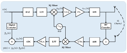
(a) Detailed system model.

(b) Digital canceler.

Fig. 1: Full-duplex transceiver system model.

An FD transceiver consisting of a local transmitter, local receiver, and two SI cancellation techniques is illustrated in Figs. 1(a) and (b). Specifically, the FD system’s design, shown in Fig. 1(a), employs an analog RF cancellation and a training-based digital cancellation in order to suppress the SI signal to the receiver noise level. The RF cancellation is applied at the first stage of the receiver chain to prevent the SI signal from saturating the receiver’s analog components (e.g., LNA, VGA, and ADC). However, the digital cancellation is employed after the ADC to remove the residual SI signal.

Let us denote the digital transmitted samples before the DAC by $x(n)$, with $n$ representing each sample index. The transmitted samples are converted to analog, filtered, and up-converted to the carrier frequency using the DAC, low pass filter (LPF), and IQ mixer, respectively. The IQ mixer, undesirably, distorts the transmitted signal due to the amplitude and gain imbalances between the I/Q components (i.e., IQ imbalance). Subsequently, the digital equivalent of the mixer’s output signal can be expressed as [References], [References]

$$x_{IQ}(n)=\frac{1}{2}(1+\psi e^{j\theta})\,x(n)+\frac{1}{2}(1-\psi e^{j\theta})\,x^{*}(n),$$ (1)

where $\psi$ and $\theta$ represent the gain and phase imbalance coefficients of the transmitter, respectively. The mixer’s output signal is then amplified by the PA, which further distorts the transmitted signal due to its non-idealities. The PA’s output signal can be expressed using the conventional parallel-Hammerstein (PH) model, described by (48) in the Appendix, as [References], [References], [References]

$$x_{PA}(n)=\sum_{\underset{p\,odd}{p=1,}}^{P}\sum_{m=0}^{M_{PA}}h{}_{m,p}\thinspace x_{IQ}(n-m)^{\frac{p+1}{2}}x_{IQ}^{*}(n-m)^{\frac{p-1}{2}},$$ (2)

where $h_{m,p}$ indicates the PA’s impulse response. In addition, $P$ and $M_{PA}$ represent the non-linearity order and the PA’s memory depth, respectively.

The PA’s output signal leaks to the receiver through the SI channel, forming the SI signal. Accordingly, at the receiver side of the FD node, there are three signals: an SI signal, a noise signal, and a far-end desired signal from another FD node. In this work, we assume, for simplicity of analysis, that there is no thermal noise, and there are no far-end desired signals from any other FD nodes [References], [References]. As such, the residual SI signal after the RF cancellation process is filtered, amplified, down-converted, and digitized using the band-pass (BPF), LNA, IQ mixer, and ADC, respectively, and can be expressed as [References]

$$y_{{}_{SI}}(n)=\sum_{\underset{p\,odd}{p=1,}}^{P}\sum_{q=0}^{p}\sum_{m=0}^{M-1}h{}_{m,q,p}\,x(n-m)^{q}x^{*}(n-m)^{p-q},$$ (3)

where $h_{m,q,p}$ represents the impulse response of a channel, including the composite effect of the PA, IQ mixer, and SI channel, whereas $M$ indicates the memory effect incorporated into the input signal by the PA and SI coupling channel.

The estimation of the aforementioned channel is performed using the least-squares (LS) approach as follows. Firstly, we formulate the matrix $\boldsymbol{X}$ with dimensions $N\times M$ from the input data $x$, where $N$ is the length of the training data. Then, the output signal $\boldsymbol{y}$ with dimension $N\times 1$ can be obtained as $\boldsymbol{y=Xh}$, where $\boldsymbol{h}$ is a vector of size $M\times 1$. In the LS method, the aim is to minimize the cost function $J(\boldsymbol{\boldsymbol{\hat{h}}})$, which can be expressed as

$$J(\boldsymbol{\boldsymbol{\hat{h}}})=\left\|\boldsymbol{y}-\boldsymbol{X}\boldsymbol{\hat{h}}\right\|^{2}=(\boldsymbol{y}-\boldsymbol{X}\boldsymbol{\hat{h}})^{H}(\boldsymbol{y}-\boldsymbol{X}\boldsymbol{\hat{h}})$$

$$\hskip 29.02179pt=\boldsymbol{y^{H}\boldsymbol{y}}-\boldsymbol{y^{H}\boldsymbol{X}\boldsymbol{\hat{h}}}-\boldsymbol{\hat{h}}^{H}\boldsymbol{\boldsymbol{X}^{H}}\boldsymbol{\boldsymbol{y}}+\boldsymbol{\hat{h}}^{H}\boldsymbol{\boldsymbol{X}^{H}}\boldsymbol{\boldsymbol{X}}\boldsymbol{\boldsymbol{\hat{h}}},$$ (4)

where $\left(.\right)^{H}$denotes the Hermitian transpose operator. By setting the derivative of this cost function with respect to $\boldsymbol{\hat{h}}$ to zero, the LS solution can be given as

$$\boldsymbol{\boldsymbol{\hat{h}}}=\left(\boldsymbol{X^{H}}\boldsymbol{X}\right)^{-1}\boldsymbol{X^{H}}\boldsymbol{y}.$$ (5)

In the digital canceler, the goal is to estimate the distortion caused by the imperfection of the transceiver hardware components and SI channel to generate an accurate replica of the SI signal $\tilde{y}_{{}_{SI}}(n)$ at the receiver. This is attained by feeding the baseband transmitted samples before the digital-to-analog conversion to a trainable-based digital canceler in order to produce such a replica. This replica is then subtracted from the SI signal after the ADC to remove the interference, and the residual SI after the digital cancellation is given by $y(n)=y_{{}_{SI}}(n)-\tilde{y}_{{}_{SI}}(n)$. The achieved SI cancellation in the digital domain can be quantified in dB as

$$\mathbb{\mathcal{C}}_{dB}=10\log_{10}\left(\frac{\sum_{n}\left|y_{{}_{SI}}(n)\right|^{2}}{\sum_{n}\left|y(n)\right|^{2}}\right)\negmedspace.$$ (6)

In this work, the digital canceler is formed by linear and non-linear trainable-based cancelers, as depicted in Fig. 1(b). The former is utilized to estimate the linear part of the SI signal based on the conventional LS channel estimation [References], whereas the latter is used to mimic the non-linear part of the SI signal using an NN model. The SI signal is then reconstructed by combining the linear and non-linear components as follows:

$$\tilde{y}_{{}_{SI}}(n)=\tilde{y}_{{}_{SI,lin}}(n)+\tilde{y}_{{}_{SI,nl}}(n),$$ (7)

where $\tilde{y}_{{}_{SI,lin}}(n)$ is the linear part of the SI signal, which can be obtained by substituting $p=1$ and $q=1$ in (3) as

$$\tilde{y}_{{}_{SI,lin}}(n)=\sum_{m=0}^{M-1}h{}_{m,1,1}\,x(n-m),$$ (8)

while $\tilde{y}_{{}_{SI,nl}}(n)$ is the non-linear part, which can be given as

$$\tilde{y}_{{}_{SI,nl}}(n)=g\left\{x\left(n\right),x\left(n-1\right),...,x\left(n-M+1\right)\right\},$$ (9)

where $g\left\{.\right\}$ represents the NN mapping function.

III Proposed Hybrid-Layers NN Architectures

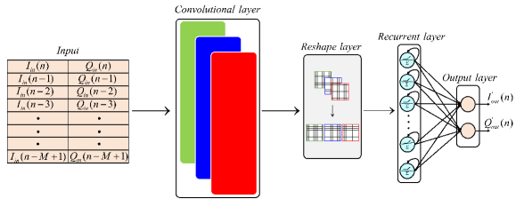
Fig. 2: Proposed HCRNN architecture.

The main function of the NN-based canceler is to provide an accurate behavior model to mimic the non-linearities and memory effect attributed to the input signal. As such, to account for such effects, TDNN or RNN-based models were employed in the literature. While the aforementioned models attain good modeling capabilities for approximating the SI in FD systems, their complexity is a considerable issue that should be addressed. A good choice for designing a low-complexity NN model is to exploit the high feature extraction along with the parameter reduction capabilities of the convolutional layer. Further, adding a recurrent layer with a sufficient number of neurons after the convolutional layer can enhance the modeling capabilities with no much increase in the computational complexity. Lastly, exploiting an additional dense layer after the recurrent layer can help to add another degree of freedom for adapting the NN settings in order to achieve the best compromise between the model performance and the computational complexity. In the next subsections, we will show how the proposed NN architectures exploit the aforementioned layers in order to build low-complexity NN-based cancelers.

III-A HCRNN Architecture

Fig. 3: Example of the basic operation of the proposed HCRNN.

The proposed HCRNN architecture is shown in Fig. 2. In the HCRNN, hybrid hidden layers are employed to detect the memory effect and non-linearity incorporated into the input signal due to the impairments of the FD transceiver and SI channel. The HCRNN is arranged in five layers: the input layer, convolutional layer, reshape layer, recurrent layer, and output layer. At the input layer, the input data is formulated into a 2D graph consisting of the I/Q components of the instantaneous and delayed versions of the input samples. Arranging the data into a 2D graph allows the input samples to be in an appropriate form that can be efficiently processed by the next convolutional layer. The convolutional layer, the first hidden layer of the HCRNN, is applied to the 2D grid in order to detect the input signal’s features with a reduced network scale. Applying the convolutional layer to the input graph comes with a considerable reduction in the computational complexity due to the weight-sharing characteristics and dimensionality reduction capabilities of the convolutional filters [References]. The convolutional layer’s output is then reordered using a reshape layer, to be processed by the next recurrent layer, which constitutes the second hidden layer of the HCRNN. The aim of the recurrent layer is to assist in learning the temporal behavior of the input signal from the localized feature map of the convolutional layer. Finally, at the output layer of the HCRNN, the I/Q components of the SI signal are estimated.

An example showing the basic operation of the proposed HCRNN, using $M=13$, three convolutional filters, and $8\times 1\times 1$ filter size, is illustrated in Fig. 3. At the convolutional layer, the input data is convolved with the filters, acting as optimizable-feature extractors, in order to detect the patterns of the input attributes. The output feature map of the $l^{th}$ filter after applying the convolution operation can be expressed as

$$\boldsymbol{F}_{c}^{l}=\begin{bmatrix}I_{in}(n)&Q_{in}(n)\\ I_{in}(n-1)&Q_{in}(n-1)\\ I_{in}(n-2)&Q_{in}(n-2)\\ .&.\\ .&.\\ I_{in}(n-M+1)&Q_{in}(n-M+1)\end{bmatrix}\otimes\begin{bmatrix}k_{1,1}^{l}&k_{1,S}^{l}\\ k_{2,1}^{l}&k_{2,S}^{l}\\ k_{3,1}^{l}&k_{3,S}^{l}\\ .&.\\ .&.\\ k_{R,1}^{l}&k_{R,S}^{l}\end{bmatrix},$$ (10)

where $l=1,2,...,L$, with $L$ denoting the number of convolutional filters. $I_{in}(n)$ and $Q_{in}(n)$ represent the I/Q components of the current sample $x(n)$, respectively, while $[I_{in}(n-1),...,I_{in}(n-M+1)]$ and $[Q_{in}(n-1),...,Q_{in}(n-M+1)]$ indicate the I/Q components of the delayed samples, respectively. In addition, $R\times S\times Z$ and $k_{i,j}^{l}$ represent the dimensions and $(i^{th},j^{th})$ entry of the $l^{th}$ convolutional filter, respectively. Finally, $\otimes$ denotes the convolution operation. It is worth mentioning that for all convolutional filters, $R\in\left\{1,2,...,M\right\}$, $S\in\left\{1,2\right\}$, and $Z=1$ since the input data is arranged into a 2D graph consisting of two columns to represent the I/Q components of the instantaneous and delayed versions of the input samples.

After performing the convolution, a bias term is added, and a non-linear activation function is applied to each element of $\boldsymbol{F}_{c}^{l}$. Accordingly, the output feature map of the $l^{th}$ convolutional filter can be expressed as

$$\boldsymbol{F}^{l}=\begin{bmatrix}f^{c}(a_{1,1}^{l}+b_{l})&f^{c}(a_{1,C}^{l}+b_{l})\\ f^{c}(a_{2,1}^{l}+b_{l})&f^{c}(a_{2,C}^{l}+b_{l})\\ f^{c}(a_{3,1}^{l}+b_{l})&f^{c}(a_{3,C}^{l}+b_{l})\\ .&.\\ .&.\\ f^{c}(a_{B,1}^{l}+b_{l})&f^{c}(a_{B,C}^{l}+b_{l})\end{bmatrix},$$ (11)

where $f^{c}(.)$ denotes the convolutional layer’s activation function, while $b_{l}$ represents the bias term associated with the $l^{th}$ convolutional filter. $B\times C$ indicates the output feature map’s dimensions, whereas $a_{i,j}^{l}$ denotes the $(i^{th},j^{th})$ entry of the feature map just after applying the convolution. With unity-stride and without zero-padding, $a_{i,j}^{l}$ can be given as

$$a_{i,j}^{l}=\sum_{r=0}^{R-1}\sum_{s=0}^{S-1}\boldsymbol{X}_{r,s+j}\boldsymbol{K}_{r,s}^{l},$$ (12)

where $\boldsymbol{X}$ and $\boldsymbol{K}^{l}$ represent the input and the $l^{th}$ convolutional filter matrices with entries described in (10), respectively.

For efficient processing of the forwarded data through the network, the output feature maps of all filters are reshaped before they are passed to the recurrent layer. More specifically, in the output feature map of each filter, there are dependencies between each column’s elements due to the temporal behavior existing in the input data. Therefore, in the proposed HCRNN, the output feature maps of all filters are reformulated using the reshape layer in order to take these dependencies into account and pass them in a sequence to the recurrent layer. Reshaping the feature maps with this mechanism enables the recurrent layer to detect the aforementioned sequence for proper modeling of the system’s temporal behavior. Based on this, the resultant feature map after the reshaping process can be expressed as

$$\boldsymbol{F}_{out}=\begin{bmatrix}\boldsymbol{F}^{1}&\boldsymbol{F}^{2}&...&\boldsymbol{F}^{L}\end{bmatrix},$$ (13)

where $\boldsymbol{F}^{1}$, $\boldsymbol{F}^{2}$, and $\boldsymbol{F}^{L}$ represent the output feature maps of the $1^{st}$, $2^{nd}$, and $L^{th}$ convolutional filters, respectively. The reshaped feature map is then passed to the recurrent layer, and the output at any time step $t$ can be expressed as

$$\boldsymbol{y}_{r}(t)=f^{r}\left(\boldsymbol{f}_{out}(t)\boldsymbol{W}_{x}+\boldsymbol{y}_{r}(t-1)\boldsymbol{W}_{y}+\boldsymbol{b}_{r}\right),$$ (14)

where $\boldsymbol{y}_{r}(t)\in\mathbb{R}^{1\times n_{hr}}$ represents the recurrent layer output at any time step $t$, with $n_{hr}$ denoting the number of recurrent layer’s neurons. Similarly, $\boldsymbol{y}_{r}(t-1)\in\mathbb{R}^{1\times n_{hr}}$ indicates the recurrent layer’s output at the previous time step $t-1$. $\boldsymbol{f}_{out}(t)\in\mathbb{R}^{1\times n_{i}}$ represents a row vector of $\boldsymbol{F}_{out}$, which is passed to the recurrent layer at time step $t$, with $n_{i}$ as the number of input features. $\boldsymbol{W}_{x}\in\mathbb{R}^{n_{i}\times n_{hr}}$ denotes the weight matrix for the connections between the input and hidden units at the current time step. Further, $\boldsymbol{W}_{y}\in\mathbb{R}^{n_{hr}\times n_{hr}}$ indicates the weight matrix for the feedback connections from the hidden units at the previous time step. Finally, $f^{r}(.)$ represents the activation function operation of the recurrent layer, whereas $\boldsymbol{b}_{r}\in\mathbb{R}^{1\times n_{hr}}$ indicates a row vector containing the bias terms of the recurrent layer neurons.

The recurrent layer’s output is then passed to the output layer, which is formed by a fully-connected (dense) layer containing two neurons. The output layer neurons are utilized to map the extracted features by the recurrent layer to the final output (i.e., estimated I/Q components of the SI signal) as follows:

$$I_{out}^{{}^{\prime}}(n)=f^{o}\left(\sum_{i=1}^{n_{hr}}\boldsymbol{W}_{o}^{1,i}\mathbf{\boldsymbol{y}}_{r}^{i}+\boldsymbol{b}_{o}^{1}\right),$$ (15)

$$Q_{out}^{{}^{\prime}}(n)=f^{o}\left(\sum_{i=1}^{n_{hr}}\boldsymbol{W}_{o}^{2,i}\boldsymbol{y}_{r}^{i}+\boldsymbol{b}_{o}^{2}\right),$$ (16)

where $f^{o}(.)$ represents the output layer’s activation function, while $\{\boldsymbol{W}_{o}^{1,i},\boldsymbol{b}_{o,}^{1}\}$ and $\{\boldsymbol{W}_{o}^{2,i},\boldsymbol{b}_{o}^{2}\}$ indicate the weight and bias terms associated with the first and second neurons of the output layer, respectively.

III-B HCRDNN Architecture

Fig. 4: Proposed HCRDNN architecture.

The network architecture of the proposed HCRDNN is depicted in Fig. 4. The key difference between the HCRDNN and HCRNN architectures is that an additional dense layer is employed after the convolutional and recurrent layers as increasing the number of hidden layers can enable building more complex NN models with reduced complexity [References]. Additionally, adding a dense layer to the HCRDNN architecture provides another degree of freedom to adapt the NN settings in order to achieve the optimum cancellation-complexity trade-off. In particular, in the HCRDNN, the convolutional layer’s hyper-parameters (e.g., number of filters, filter size) and the number of neurons in the recurrent and dense layers are jointly adjusted to achieve a considerable cancellation performance with a significant computational complexity reduction.

The output of the $u^{th}$ neuron at the dense layer of the HCRDNN can be expressed as

$$y_{d}^{u}=f^{d}\left(\sum_{i=1}^{n_{hr}}\boldsymbol{W}_{d}^{u,i}\boldsymbol{y}_{r}^{i}+\boldsymbol{b}_{d}^{u}\right),$$ (17)

where $f^{d}(.)$ indicates the activation function of the dense layer, while $\{\boldsymbol{W}_{d}^{u,i},\boldsymbol{b}_{d,}^{u}\}$ represent the weight and bias terms associated with the $u^{th}$ neuron in the dense layer, respectively. The dense layer’s output is then passed to the output layer to estimate the I/Q components of the SI signal as (15) and (16).

After predicting $I_{out}^{{}^{\prime}}(n)$ and $Q_{out}^{{}^{\prime}}(n)$, the MSE is calculated as a cost function to measure how well the proposed NN models predict the actual outputs as follows:

$$E=\frac{1}{2N}\sum_{n=1}^{N}\left(\left[I_{out}(n)-I_{out}^{{}^{\prime}}(n)\right]^{2}+\left[Q_{out}(n)-Q_{out}^{{}^{\prime}}(n)\right]^{2}\right),$$ (18)

where $\{I_{out}(n),$ $I_{out}(n)\}$ and $\{I_{out}^{{}^{\prime}}(n),$ $Q_{out}^{{}^{\prime}}(n)\}$ represent the actual and predicted values of the I/Q components of the SI signal, receptively, whereas $N$ denotes the number of training observations, as stated before in Section II. During the HCRNN and HCRDNN models’ training, the convolutional, recurrent, and dense layers’ weights and biases are set to minimize this cost function.

After the training process, the proposed NNs are employed to provide non-linear SI cancellation as part of the digital cancellation in the FD transceiver, as illustrated in Fig. 1(b).

IV Complexity Analysis

In this section, the computational complexity and memory requirements of the polynomial and proposed NN-based cancelers are analyzed in terms of the number of computations and memory usage of the linear and non-linear cancelers required to provide the total SI cancellation (i.e., the summation of linear and non-linear cancellations). In particular, in this work, the computational complexity is assessed in terms of the number of FLOPs used to perform the linear and non-linear cancellation processes. Moreover, the memory usage requirements are assessed in terms of the number of stored parameters utilized to achieve the total cancellation. In this analysis, we focus on evaluating the complexity of the polynomial and proposed NN-based cancelers in the real-time inference stage since powerful processing units can be employed to perform the training process offline.

IV-A Linear Canceler Complexity

In this subsection, we calculate the number of FLOPs required to implement the linear canceler in terms of the number of RV multiplications and additions. From (8), the linear canceler requires $M$ complex multiplications and $M-1$ complex additions to perform the linear cancellation. Using the assumption that each complex addition is implemented by two real additions, and each complex multiplication is executed using three real multiplications and five real additions [References], the number FLOPs of the linear canceler can be expressed as

$$\mathscr{\mathcal{F}_{\mathit{lin}}}=\underset{\chi_{mul,lin}^{\Re}}{\underbrace{3M}}+\underset{\text{$\chi_{add,lin}^{\mathfrak{\mathbb{\Re}}}$}}{\underbrace{7M-2}},$$ (19)

where $\chi_{mul,lin}^{\Re}$ and $\chi_{add,lin}^{\mathfrak{\mathbb{\Re}}}$ represent the number of real multiplications and additions required for the linear canceler, respectively, while $M$ denotes the memory effect incorporated into the input signal by the PA and SI channel, as stated before. Similarly, from (8), the memory requirements of the linear canceler is evaluated as a function of the number of stored parameters, which can be expressed as

$$\mathcal{P}_{lin}=2M.$$ (20)

IV-B Non-Linear Canceler Complexity

In this subsection, the number of FLOPs and parameters required for non-linear cancellation using polynomial and NN-based cancelers are analyzed.

IV-B1 Polynomial-based Canceler Complexity

Using the previous assumptions, it can be deduced from (3) that the number of RV multiplications and additions required for the non-linear polynomial-based canceler can be expressed as [References], [References]

$$\chi_{mul,poly}^{\mathfrak{\mathbb{\Re}}}=3M\left\{\left(\frac{P+1}{2}\right)\left(\frac{P+1}{2}+1\right)-1\right\},$$ (21)

$$\chi_{add,poly}^{\mathfrak{\mathbb{\Re}}}=7M\left\{\left(\frac{P+1}{2}\right)\left(\frac{P+1}{2}+1\right)-1\right\}.$$ (22)

Similarly, the number of parameters of the non-linear polynomial-based canceler can be expressed as [References], [References]

$$\thinspace\thinspace\thinspace\thinspace\thinspace\thinspace\thinspace\thinspace\thinspace\thinspace\thinspace\thinspace\thinspace\thinspace\thinspace\mathcal{P}_{poly}=2M\left\{\left(\frac{P+1}{2}\right)\left(\frac{P+1}{2}+1\right)-1\right\}.$$ (23)

IV-B2 NN-based Canceler Complexity

For the proposed non-linear HCRNN-based canceler, the number of FLOPs can be expressed as

$$\mathscr{\mathcal{F}_{\mathit{HCRNN}}}=\mathcal{F^{\mathit{c}}}+\mathcal{F^{\mathit{r}}}+\mathcal{F^{\mathit{o}}},$$ (24)

where $\mathcal{F}^{\mathit{c}}$, $\mathcal{F}^{\mathit{r}}$, and $\mathcal{F}^{\mathit{o}}$ represent the number of FLOPs required for the convolutional, recurrent, and output layers of the HCRNN, respectively. Firstly, for the convolutional layer, $\mathcal{F}^{\mathit{c}}$ can be expressed as

$\underset{\text{ \thinspace\thinspace\thinspace\thinspace\thinspace\thinspace\thinspace\thinspace\thinspace\thinspace\thinspace\thinspace\thinspace\thinspace\thinspace\thinspace\thinspace\thinspace\thinspace\thinspace\thinspace\thinspace\thinspace}\textrm{Ter$\textrm{m}_{1}^{c}$}}{\mathcal{F^{\mathit{c}}}=\underbrace{\left(2\left\{R\times S\times Z\right\}-1\right)\left(B\times C\times L\right)}}$

$$\thinspace\thinspace\thinspace\thinspace\thinspace\thinspace\thinspace\thinspace\thinspace\thinspace\thinspace\thinspace\thinspace\thinspace\thinspace\thinspace\thinspace\thinspace\thinspace\thinspace\thinspace\thinspace\thinspace\thinspace\thinspace\thinspace\thinspace\thinspace\thinspace\thinspace\thinspace\thinspace\thinspace\thinspace\thinspace\thinspace\thinspace\underset{\text{\thinspace\thinspace\thinspace\thinspace\thinspace\thinspace\thinspace\thinspace\thinspace\thinspace\thinspace}\textrm{Ter$\textrm{m}_{2}^{c}$}}{+\underbrace{\mathcal{F^{\mathit{act}}}\times\left(B\times C\times L\right)}}+\underset{\text{\thinspace\thinspace}\textrm{Ter$\textrm{m}_{3}^{c}$}}{\underbrace{\left(B\times C\times L\right)}},$$ (25)

where $\textrm{Ter}\textrm{m}_{1}^{c}$ represents the number of RV multiplications and additions required to convolve the 2D graph of the input data with $L$ convolutional filters. $\textrm{Ter}\textrm{m}_{2}^{c}$ denotes the number of RV operations (multiplications + additions) required for applying the activation functions at each element of the output feature map after the convolution process. $\textrm{Ter}\textrm{m}_{3}^{c}$ indicates the number of real additions required for adding the bias values. Finally, $\mathcal{F^{\mathit{act}}}$ represents the number of real operations needed to evaluate each activation function, which mainly depends on the activation function type.

In this work, we consider the rectified linear unit ($ReLU$), $Sigmoid$, and hyperbolic tangent ($tanh$) activation functions, which are defined as [References]

$$ReLU(z) =\max(0,z),$$ (26a)

$$Sigmoid(z) =\frac{1}{e^{-z}+1},$$ (26b)

$$tanh(z) =\frac{e^{z}-e^{-z}}{e^{z}+e^{-z}}.$$ (26c)

By assuming that each real operation (e.g., multiplication, division, addition, subtraction, and exponentiation) costs one FLOP [References], [References], the number of FLOPs required to implement each of the aforementioned activation functions can be expressed as

$$\mathcal{F^{\mathit{act}}}=\begin{cases}1,&\textrm{ \thinspace\thinspace\thinspace\thinspace if }ReLU\\ 4,&\textrm{ \thinspace\thinspace\thinspace\thinspace if }Sigmoid\\ 6,&\textrm{ \thinspace\thinspace\thinspace\thinspace if }tanh\end{cases}.$$ (27)

Secondly, the number of FLOPs required for the recurrent layer can be expressed as

$$\underset{\text{ }}{\underset{\text{ \thinspace\thinspace\thinspace\thinspace\thinspace\thinspace\thinspace\thinspace\thinspace\thinspace\thinspace\thinspace\thinspace\thinspace\thinspace\thinspace\thinspace\thinspace\thinspace\thinspace\thinspace\thinspace\thinspace{Ter$\textrm{m}_{1}^{r}$}}}{\mathcal{F^{\mathit{r}}}=\underbrace{2n_{hr}\left(n_{i}+n_{hr}-\frac{1}{2}\right)}}}\underset{\text{\thinspace\thinspace\thinspace\thinspace\thinspace\thinspace\thinspace\thinspace\thinspace\thinspace\thinspace\thinspace\thinspace{Ter$\textrm{m}_{2}^{r}$}}}{+\underbrace{\mathcal{F^{\mathit{act}}}\times n_{hr}}}+\underset{\text{\thinspace\thinspace{Ter$\textrm{m}_{3}^{r}$}}}{\underbrace{n_{hr}}},$$ (28)

where $\textrm{Ter}\textrm{m}_{1}^{r}$ represents the number of RV operations associated with multiplying the weight matrices $\boldsymbol{W}_{x}$ and $\boldsymbol{W}_{y}$ in (14) with their corresponding inputs, while $\textrm{Ter}\textrm{m}_{2}^{r}$ and $\textrm{Ter}\textrm{m}_{3}^{r}$ indicate the number of real operations required for applying the activation functions and adding the biases at each neuron of the recurrent layer, respectively.

Finally, the output layer’s FLOPs can be expressed as

$$\underset{\text{\thinspace\thinspace\thinspace\thinspace\thinspace\thinspace\thinspace\thinspace\thinspace\thinspace\thinspace\thinspace\thinspace\thinspace\thinspace\thinspace\thinspace\thinspace\thinspace\thinspace\thinspace\thinspace\thinspace\thinspace\thinspace\thinspace{Ter$\textrm{m}_{1}^{o}$}}}{\mathcal{F^{\mathit{o}}}=\underbrace{n_{ho}\left(2n_{hr}-1\right)}}\underset{\text{\thinspace\thinspace\thinspace\thinspace\thinspace\thinspace\thinspace\thinspace\thinspace\thinspace\thinspace{Ter$\textrm{m}_{2}^{o}$}}}{+\underbrace{\mathcal{F^{\mathit{act}}}\times n_{ho}}}+\underset{\text{\thinspace\thinspace{Ter$\textrm{m}_{3}^{o}$}}}{\underbrace{n_{ho}}},$$ (29)

where $n_{ho}$ represents the number of output layer’s neurons. $\textrm{Ter}\textrm{m}_{1}^{o}$ denotes the number of RV operations required to calculate the weighted sum of inputs at the output layer neurons. $\textrm{Ter}\textrm{m}_{2}^{o}$ and $\textrm{Ter}\textrm{m}_{3}^{o}$ indicate the number of real operations associated with employing the activation functions and adding the bias terms at each neuron of the output layer, respectively.

The number of parameters of the proposed HCRNN architecture can be given as

$$\mathcal{P}_{HCRNN}=\mathcal{P^{\mathit{c}}}+\mathcal{P^{\mathit{r}}+\mathcal{P^{\mathit{o}}}},$$ (30)

where $\mathcal{P^{\mathit{c}}}$, $\mathcal{P^{\mathit{r}}}$, and $\mathcal{P^{\mathit{o}}}$ represent the number of parameters of the convolutional, recurrent, and output layers, respectively, which can be expressed as

$$\mathcal{P^{\mathit{c}}} =L\left(R\times S\times Z+1\right),$$ (31a)

$$\mathcal{P}^{\mathit{r}} =n_{hr}\left(n_{i}+n_{hr}+1\right),$$ (31b)

$$\mathcal{P^{\mathit{o}}} =n_{ho}\left(n_{hr}+1\right).$$ (31c)

Using the same mathematical formulation, the number of FLOPs of the proposed HCRDNN can be calculated as

$$\mathscr{\mathcal{F}_{\mathit{HCRDNN}}}=\mathcal{F^{\mathit{c}}}+\mathcal{F^{\mathit{r}}}+\mathcal{F^{\mathit{d}}}+\mathcal{F^{\mathit{o}}},$$ (32)

where $\mathcal{F}^{\mathit{c}}$ and $\mathcal{F}^{\mathit{r}}$ represent the convolutional and recurrent layers’ FLOPs, which can be determined using (25) and (28), respectively. $\mathcal{F}^{\mathit{o}}$ indicates the output layer’s FLOPs, which can be calculated by replacing $n_{hr}$ by $n_{hd}$ in (29), whereas $\mathcal{F}^{\mathit{d}}$ denotes the dense layer’s FLOPs, which can be expressed as

$$\underset{\text{\thinspace\thinspace\thinspace\thinspace\thinspace\thinspace\thinspace\thinspace\thinspace\thinspace\thinspace\thinspace\thinspace\thinspace\thinspace\thinspace\thinspace\thinspace\thinspace\thinspace\thinspace\thinspace\thinspace\thinspace\thinspace\thinspace{Ter$\textrm{m}_{1}^{d}$}}}{\mathcal{F^{\mathit{d}}}=\underbrace{n_{hd}\left(2n_{hr}-1\right)}}\underset{\text{\thinspace\thinspace\thinspace\thinspace\thinspace\thinspace\thinspace\thinspace\thinspace\thinspace\thinspace{Ter$\textrm{m}_{2}^{d}$}}}{+\underbrace{\mathcal{F^{\mathit{act}}}\times n_{hd}}}+\underset{\text{\thinspace\thinspace{Ter$\textrm{m}_{3}^{d}$}}}{\underbrace{n_{hd}}},$$ (33)

where $\textrm{Ter}\textrm{m}_{1}^{d}$, $\textrm{Ter}\textrm{m}_{2}^{d}$, and $\textrm{Ter}\textrm{m}_{3}^{d}$ represent the number of real operations required for calculating the weighted sum of inputs, applying the activation functions, and summing the biases at the dense layer neurons, respectively.

The number of parameters of the HCRDNN can be given as

$$\mathcal{P}_{HCRDNN}=\mathcal{P^{\mathit{c}}}+\mathcal{P^{\mathit{r}}+\mathcal{P^{\mathit{d}}}}+\mathcal{P^{\mathit{o}}},$$ (34)

where $\mathcal{P}^{\mathit{c}}$ and $\mathcal{P}^{\mathit{r}}$ represent the convolutional and recurrent layers’ parameters given by (31a) and (31b), respectively, while $\mathcal{P}^{\mathit{o}}$ indicates the output layer’s parameters, which can be evaluated by replacing $n_{hr}$ by $n_{hd}$ in (31c). Lastly, $\mathcal{P}^{\mathit{d}}=n_{hd}\left(n_{hr}+1\right)$ is the number of dense layer parameters.

For the RV-TDNN [References], [References], the number of FLOPs and parameters can be expressed as

$$\mathscr{\mathcal{F}_{\mathit{RV-TDNN}}}=\sum_{j=2}^{\mathcal{L}}2n_{j-1}n_{j}+\mathcal{F^{\mathit{act,j}}}n_{j},$$ (35)

$$\mathcal{P}_{RV-TDNN}=\sum_{j=2}^{\mathcal{L}}n_{j-1}n_{j}+n_{j},$$ (36)

where $\mathcal{L}$ indicates the number of layers of the RV-TDNN, including the input, hidden, and output layers. $n_{j}$ is the number of neurons in the $j^{th}$ layer, with $n_{1}$ and $n_{\mathcal{L}}$ representing the number of input and output layers’ neurons, respectively. $\mathcal{\mathcal{F^{\mathit{act,j}}}}$ denotes the number of operations required to apply the activation function at each of the $j^{th}$ layer’s neurons.

Similarly, for the RNN [References], the number of FLOPs and parameters can be given by

$$\mathscr{\mathcal{F}_{\mathit{RNN}}}=\sum_{j=2}^{\mathcal{L}}2n_{j-1}n_{j}+2n_{j}^{2}+\mathcal{F^{\mathit{act,j}}}n_{j}-2n_{\mathcal{L}}^{2},$$ (37)

$$\mathcal{P}_{RNN}=\sum_{j=2}^{\mathcal{L}}n_{j-1}n_{j}+n_{j}^{2}+n_{j}-n_{\mathcal{L}}^{2},$$ (38)

with $n_{1}$ denotes the number of RNN inputs at each time step.

For the CV-TDNN [References], using the previous implementation assumptions for the CV additions and multiplications, the number of FLOPs and parameters can be given by

$$\mathscr{\mathcal{F}_{\mathit{CV-TDNN}}}=10\left\{\sum_{j=2}^{\mathcal{L}}n_{j-1}n_{j}\right\}+\mathcal{F^{\mathit{act,j}}}n_{j},$$ (39)

$$\mathcal{P}_{CV-TDNN}=2\left\{\sum_{j=2}^{\mathcal{L}}n_{j-1}n_{j}+n_{j}\right\}.\hskip 17.07182pt$$ (40)

For the LWGS [References] employing $n_{i}$ CV inputs and a single hidden layer with $n_{h}$ neurons, the number of FLOPs and parameters can be expressed as

$$\mathscr{\mathcal{F}_{\mathit{LWGS}}}=10\left\{\left(\sum_{j=1}^{\mathcal{\mathit{n_{h}}}}j\right)+\mathcal{\mathit{n_{i}}}\right\}+\mathcal{F^{\mathit{act}}}n_{h},$$ (41)

$$\mathcal{P}_{LWGS}=2\left\{\left(\sum_{j=1}^{\mathcal{\mathit{n_{h}}}}j\right)+\mathcal{\mathit{n_{i}}}+\mathcal{\mathit{n_{h}}+}1\right\}.$$ (42)

Likewise, for the MWGS [References] employing $n_{i}$ CV inputs, a $\mathcal{W}$ window size, and a single hidden layer with $n_{h}$ neurons, the number of FLOPs and parameters can be obtained as follows:

$$\mathscr{\mathcal{F}_{\mathit{MWGS}}}=10\left\{\mathcal{\mathit{n_{i}}}+\mathcal{W}\left(\mathcal{\mathit{n_{h}}}-1\right)+\mathcal{\mathit{n_{h}}}\right\}+\mathcal{F^{\mathit{act}}}n_{h},$$ (43)

$$\mathcal{P}_{MWGS}=2\left\{\mathcal{\mathit{n_{i}}}+\mathcal{W}\left(\mathcal{\mathit{n_{h}}}-1\right)+2\mathcal{\mathit{n_{h}}}+1\right\}.$$ (44)

Finally, the total number of FLOPs of any of the aforementioned NN-based cancelers can be expressed as

$$\mathscr{\mathcal{F}_{\mathit{NN-\mathcal{C}}}}=\mathscr{\mathcal{F}_{\mathit{lin}}}+\mathscr{\mathcal{F}_{\mathit{NN}}}+2,$$ (45)

where $\mathscr{\mathcal{F}_{\mathit{lin}}}$ represents the linear canceler complexity, which can be calculated by (19), while $\mathscr{\mathscr{\mathcal{F}_{\mathit{NN}}}}$ indicates the NN complexity (e.g., $\mathscr{\mathcal{F}_{\mathit{HCRNN}}}$, $\mathscr{\mathcal{F}_{\mathit{HCRDNN}}}$, $\mathscr{\mathcal{F}_{\mathit{RV-TDNN}}}$). The two FLOPs added in (45) represent the number of real additions required to sum the outputs of the linear and non-linear cancelers in (8) and (9), respectively [References].

V Optimum Settings of the Proposed HCRNN and HCRDNN Architectures

In this section, the optimum settings for training the proposed HCRNN and HCRDNN architectures are obtained. Specifically, the number of convolutional filters, filter size, number of recurrent and dense layers’ neurons, activation functions in each layer, learning rate, batch size, and training optimizer are selected in such a way that results in a proper cancellation performance while maintaining low computational complexity. In the following, we firstly describe the dataset employed to train the proposed NN architectures, then the network settings for the training process are optimized.

V-A Training Dataset

In the following experiments, the public dataset employed in [References] and [References] is utilized to train and verify the proposed NN architectures. The dataset is produced using a realistic FD test-bed, which generates a 10 MHz quadrature phase-shift keying modulated-orthogonal frequency division multiplexing (OFDM) signal with an average transmit power of 10 dBm. The OFDM signal employs 1024 sub-carriers and is sampled at 20 MHz. The generated dataset contains 20,480 time-domain baseband samples, which we split into two distinct parts. The first part is used for training and consists of 90% of samples, whereas the second is employed for verification and contains the rest 10%. The employed hardware test-bed provides 53 dB passive analog RF cancellation using physical separation between the transmit and receive antennas; hence, in this work, no further active analog cancellation techniques are employed since the use of digital cancellation after passive analog suppression is adequate to bring the SI signal’s power down to the receiver’s noise level [References], [References]. A summary of the parameters employed to generate the aforementioned dataset is presented in Table. I.

TABLE I: Summary of the parameters employed to generate the dataset utilized for training and verifying the proposed NN architectures.

Parameter	Value
Type of modulation	QPSK-modulated OFDM
Pass-band bandwidth	10 MHz
Number of carriers	1024
Sampling frequency	20 MHz
Average transmit power	10 dBm
Passive analog suppression	53 dB
Active analog suppression	N/A
Total analog cancellation	53 dB
Dataset size	20,480 samples

TABLE II: Selection of the optimum configuration of the proposed HCRNN.

Config. #	# Filters	Filter size	# Rec. neurons	SI Canc. (dB)	Complexity		Config. #	# Filters	Filter size	# Rec. neurons	SI Canc. (dB)	Complexity
					# Par.	# FLOPs						# Par.	# FLOPs
1	2	4$\times$1$\times$1	6	43.01	116	640	17	2	4$\times$1$\times$1	10	44.18	208	820
2	2	8$\times$1$\times$1	6	42.60	124	688	18	2	9$\times$1$\times$1	10	44.05	218	840
3	2	6$\times$1$\times$1	7	42.92	140	735	19	2	10$\times$1$\times$1	10	44.06	220	796
4	2	4$\times$1$\times$1	8	43.75	158	722	20	2	11$\times$1$\times$1	10	44.19	222	736
5	2	5$\times$1$\times$1	8	43.81	160	758	21	2	12$\times$1$\times$1	10	44.31	224	660
6	2	8$\times$1$\times$1	8	43.89	166	770	22	3	11$\times$1$\times$1	6	43.66	154	718
7	2	10$\times$1$\times$1	8	43.89	170	698	23	3	12$\times$1$\times$1	6	43.97	157	604
8	2	11$\times$1$\times$1	8	43.68	172	638	24	3	11$\times$1$\times$1	7	44.11	176	761
9	2	5$\times$1$\times$1	9	44.03	184	805	25	3	12$\times$2$\times$1	7	43.54	194	599
10	2	6$\times$1$\times$1	9	44.03	186	825	26	3	11$\times$1$\times$1	8	44.10	200	808
11	2	7$\times$1$\times$1	9	44.02	188	829	27	3	12$\times$1$\times$1	9	44.44	229	745
12	2	9$\times$1$\times$1	9	43.93	192	789	28	3	13$\times$1$\times$1	9	43.94	232	607
13	2	10$\times$1$\times$1	9	44.08	194	745	29	3	11$\times$2$\times$1	9	43.85	232	796
14	2	12$\times$1$\times$1	9	44.23	198	609	30	3	12$\times$2$\times$1	9	44.09	238	685
15	2	12$\times$2$\times$1	9	43.61	204	569	31	3	12$\times$1$\times$1	10	44.49	257	800
16	2	3$\times$1$\times$1	10	44.06	206	768	32	3	12$\times$2$\times$1	10	44.12	299	734

TABLE III: Selection of the optimum configuration of the proposed HCRDNN.

Config. #	# Filters	Filter size	# Rec. neurons	# Dense neurons	SI Canc. (dB)	Complexity		Config. #	# Filters	Filter size	# Rec. neurons	# Dense neurons	SI Canc. (dB)	Complexity
						# Par.	# FLOPs							# Par.	# FLOPs
1	2	7$\times$1$\times$1	5	9	44.10	166	789	17	2	12$\times$1$\times$1	8	10	44.42	268	740
2	2	9$\times$1$\times$1	5	10	44.10	178	755	18	2	12$\times$1$\times$1	9	7	44.42	264	734
3	2	12$\times$1$\times$1	5	11	44.29	192	590	19	2	12$\times$1$\times$1	9	8	44.50	276	757
4	2	9$\times$1$\times$1	5	12	44.14	194	785	20	2	12$\times$1$\times$1	9	9	44.42	288	780
5	2	10$\times$1$\times$1	5	12	44.18	196	741	21	2	12$\times$1$\times$1	10	6	44.46	282	770
6	2	12$\times$1$\times$1	5	12	44.27	200	605	22	3	12$\times$1$\times$1	5	6	44.11	175	635
7	2	10$\times$1$\times$1	6	9	44.09	197	745	23	3	12$\times$1$\times$1	5	7	44.10	183	650
8	2	12$\times$1$\times$1	6	9	44.22	201	609	24	3	12$\times$1$\times$1	5	8	44.15	191	665
9	2	11$\times$1$\times$1	6	10	44.11	208	702	25	3	12$\times$1$\times$1	5	10	44.24	207	695
10	2	10$\times$1$\times$1	6	11	44.25	215	779	26	3	12$\times$1$\times$1	5	11	44.17	215	710
11	2	11$\times$1$\times$1	6	11	44.23	217	719	27	3	12$\times$1$\times$1	5	12	44.41	223	725
12	2	12$\times$1$\times$1	6	11	44.26	219	643	28	3	12$\times$1$\times$1	6	6	44.28	199	682
13	2	11$\times$1$\times$1	7	11	44.21	246	776	29	3	12$\times$1$\times$1	6	8	44.22	217	716
14	2	12$\times$1$\times$1	7	11	44.44	248	700	30	3	12$\times$1$\times$1	6	9	44.36	226	733
15	2	12$\times$1$\times$1	7	12	44.44	258	719	31	3	12$\times$1$\times$1	6	11	44.40	244	767
16	2	12$\times$1$\times$1	8	9	44.41	257	719	32	3	12$\times$1$\times$1	6	12	44.39	253	784

V-B Optimum Configuration

The process of selecting the optimum configuration of the proposed HCRNN (e.g., number of convolutional filters, filter size, number of recurrent layer’s neurons) is analyzed as given in Table II. To that end, we test two values for the convolutional filters $L\in\{2,3\}$ and change the filter size dimensions such that $R\in\{2,3,...,13\}$, $S\in\{1,2\}$, and $Z=1$ for all filters. Moreover, we consider $n_{hr}\in\{4,5,...,10\}$ for the number of neurons in the recurrent layer. Since there is a large number of combinations between $L$, $R$, $S$, $Z$, and $n_{hr}$, we only show the NN configurations that achieve the best cancellation-complexity trade-off in Table II. Specifically, in this work, choosing the optimum configuration of the HCRNN is based on the criterion of achieving a similar or comparable cancellation performance to the polynomial canceler with $P=5$ while maintaining a lower implementation complexity. Based on this, it can be observed from Table II that the HCRNN configuration with three convolutional filters, $12\times 1\times 1$ filter size, and nine neurons in the recurrent layer achieves the target cancellation of the polynomial canceler. Besides, it attains the best compromise between the cancellation performance and implementation complexity compared to its other counterparts. Similarly, the selection of the optimum configuration of the proposed HCRDNN is explored in Table III.² In this case, we test the number of filters $L\in\{2,3\}$, filter dimensions $R\in\{2,3,...,13\}$, $S\in\{1,2\}$, and $Z=1$, recurrent layer’s neurons $n_{hr}\in\{4,5,...,10\}$, and dense layer’s neurons $n_{hd}\in\{4,5,...,12\}$. As can be seen from Table III, two configurations of the proposed HCRDNN achieve the best compromise among the cancellation performance, number of FLOPs, and parameters. The first configuration (i.e., HCRDNN 1) employs two convolutional filters, $12\times 1\times 1$ filter size, seven neurons in the recurrent layer, and eleven neurons in the dense layer. However, the second (i.e., HCRDNN 2) utilizes three convolutional filters, $12\times 1\times 1$ filter size, five neurons in the recurrent layer, and twelve neurons in the dense layer. It is worth mentioning here that from Tables II and III, the filter size of $12\times 1\times 1$ is shown to be the best size for the optimizable convolutional filters employed in both the HCRNN and HCRDNN architectures. Moreover, it is worth noting that using an additional dense layer in the proposed HCRDNN 1 and HCRDNN 2 reduces the number of neurons in the recurrent layer from 9 to 7 and 5 neurons, respectively, compared to the HCRNN architecture; this significantly affects the computational complexity of the HCRDNN model.

TABLE IV: Optimum activation functions of the proposed HCRNN.

Config. #	Conv. layer	Rec. layer	SI Canc. (dB)	FLOPs
1	$tanh$	$tanh$	44.61	850
2	$tanh$	$ReLU$	44.50	805
3	$tanh$	$Sigm$	44.15	832
4	$ReLU$	$tanh$	44.37	790
5	$\boldsymbol{ReLU}$	$\boldsymbol{ReLU}$	44.44	745
6	$ReLU$	$Sigm$	44.41	772
7	$Sigm$	$tanh$	44.27	826
8	$Sigm$	$ReLU$	43.65	781
9	$Sigm$	$Sigm$	43.12	808

TABLE V: Optimum activation functions of the proposed HCRDNN.

Config. #	Conv. layer	Rec. layer	Dense layer	SI Canc. (dB)		FLOPs
				HCRDNN 1	HCRDNN 2	HCRDNN 1	HCRDNN 2
1	$tanh$	$tanh$	$tanh$	44.41	44.33	830	870
2	$tanh$	$tanh$	$ReLU$	44.49	44.57	775	810
3	$tanh$	$tanh$	$Sigm$	44.21	43.98	808	846
4	$tanh$	$ReLU$	$tanh$	44.40	44.30	795	845
5	$tanh$	$ReLU$	$ReLU$	44.36	44.34	740	785
6	$tanh$	$ReLU$	$Sigm$	44.14	43.98	773	821
7	$tanh$	$Sigm$	$tanh$	43.98	44.05	816	860
8	$tanh$	$Sigm$	$ReLU$	44.13	44.34	761	800
9	$tanh$	$Sigm$	$Sigm$	43.96	44.09	794	836
10	$ReLU$	$tanh$	$tanh$	44.48	44.24	790	810
11	$ReLU$	$tanh$	$ReLU$	44.54	44.48	735	750
12	$ReLU$	$tanh$	$Sigm$	44.17	43.88	768	786
13	$ReLU$	$ReLU$	$tanh$	44.36	44.14	755	785
14	$\boldsymbol{ReLU}$	$\boldsymbol{ReLU}$	$\boldsymbol{ReLU}$	44.44	44.41	700	725
15	$ReLU$	$ReLU$	$Sigm$	44.24	43.92	733	761
16	$ReLU$	$Sigm$	$tanh$	44.34	43.89	776	800
17	$ReLU$	$Sigm$	$ReLU$	44.31	44.26	721	740
18	$ReLU$	$Sigm$	$Sigm$	44.11	43.95	754	776
19	$Sigm$	$tanh$	$tanh$	44.08	43.89	814	846
20	$Sigm$	$tanh$	$ReLU$	44.04	44.07	759	786
21	$Sigm$	$tanh$	$Sigm$	43.90	43.59	792	822
22	$Sigm$	$ReLU$	$tanh$	43.46	42.78	779	821
23	$Sigm$	$ReLU$	$ReLU$	43.95	43.63	724	761
24	$Sigm$	$ReLU$	$Sigm$	43.84	43.21	757	797
25	$Sigm$	$Sigm$	$tanh$	42.53	41.98	800	836
26	$Sigm$	$Sigm$	$ReLU$	43.02	43.54	745	776
27	$Sigm$	$Sigm$	$Sigm$	42.97	42.94	778	812

V-C Optimum Activation Functions

In this subsection, we test the cancellation performance and computational complexity of the proposed HCRNN and HCRDNN using different activation functions in the convolutional, recurrent, and dense (if any) layers and select the optimum combination of activation functions that results in the best cancellation-complexity trade-off. Specifically, in Table IV, we evaluate the performance of the optimum HCRNN configuration, obtained in the previous subsection, using different activation functions. As seen from Table IV, the HCRNN with the $ReLU$ activation function in both convolutional and recurrent layers achieves the target cancellation of the polynomial canceler and provides the best compromise between the cancellation and complexity performances. It can also be inferred from Table IV that using the $tanh$ activation function in the hidden layers of HCRNN only enhances the SI cancellation by 0.17 dB at the cost of augmenting the FLOPs by 14% compared to the $ReLU$ activation function. Hence, in this work, we employ the $ReLU$ activation function for the HCRNN as it provides the best cancellation-complexity trade-off.

Likewise, in Table V, we test the optimum configurations of the HCRDNN using various activation functions. As can be observed, using the $ReLU$ activation function in the convolutional, recurrent, and dense layers attains the best cancellation-complexity trade-off for both HCRDNN architectures.

V-D Optimum Learning Rate

The effect of varying the learning rate on the cancellation performance of the proposed HCRNN and HCRDNN-based cancelers is analyzed in Table VI. It can be inferred that using a learning rate of 5$\times$1$0^{-3}$ achieves the best cancellation performance for both the proposed HCRNN and HCRDNN architectures compared to the other learning rates.

V-E Optimum Batch Size

Similarly, in this subsection, we test the effect of varying the batch size on the performance of the proposed HCRNN and HCRDNN-based cancelers. Herein, we consider many values for the batch size, and we only show the batch sizes that result in the best cancellation performance in Table VII. As can be observed, employing batch size values of 62 and 158 provide the best cancellation performance for the proposed HCRNN and HCRDNN architectures, respectively.

V-F Selected Optimizer

The cancellation performance of the proposed HCRNN and HCRDNN-based cancelers is analyzed using different optimizers, as illustrated in Table VIII. In this work, we test the stochastic gradient descent (SGD), adaptive moment estimation (Adam), root mean square propagation (RMSprop), adaptive delta (Adadelta), and adaptive max-pooling (Adamax) optimizers. As seen from Table VIII, the Adam optimization algorithm attains the best performance for the HCRNN and HCRDNN compared to the other optimization techniques.

Based on the aforementioned subsections, the optimum settings for training the proposed HCRNN and HCRDNN architectures are summarized in Table IX.

TABLE VI: Optimum learning rate of the proposed HCRNN and HCRDNN.

Learning rate	$\mathbf{1\times 10^{-2}}$	$\mathbf{5\times 10^{-3}}$	$\mathbf{1\times 10^{-3}}$	$\mathbf{5\times 10^{-4}}$	$\mathbf{1\times 10^{-4}}$
Network	SI Cancellation (dB)
HCRNN	44.36	44.44	44.12	43.64	38.90
HCRDNN 1	44.28	44.44	43.65	42.92	39.11
HCRDNN 2	44.22	44.41	44.01	43.26	39.22

TABLE VII: Optimum batch size of the proposed HCRNN and HCRDNN.

Batch size	22	62	158	256	512
Network	SI Cancellation (dB)
HCRNN	44.37	44.50	44.44	44.40	44.44
HCRDNN 1	44.17	44.38	44.44	44.39	44.28
HCRDNN 2	44.22	44.29	44.41	44.37	44.31

TABLE VIII: Selected optimizer of the proposed HCRNN and HCRDNN.

Optimizer	SGD	Adam	RMSprop	Adadelta	Adamax
Network	SI Cancellation (dB)
HCRNN	41.11	44.50	44.23	37.80	44.36
HCRDNN 1	38.37	44.44	43.97	37.84	43.93
HCRDNN 2	38.73	44.41	43.89	37.83	43.95

TABLE IX: Optimum settings of the proposed HCRNN and HCDRNN.

Structure	HCRNN	HCRDNN 1	HCRDNN 2
# Filters	3	2	3
Filter size	12$\times$1$\times$1	12$\times$1$\times$1	12$\times$1$\times$1
# Rec. neurons	9	7	5
# Dense neurons	N/A	11	12
Conv. activation	$ReLU$	$ReLU$	$ReLU$
Rec. activation	$ReLU$	$ReLU$	$ReLU$
Dense activation	N/A	$ReLU$	$ReLU$
Learning rate	5$\times$1$0^{-3}$	5$\times$1$0^{-3}$	5$\times$1$0^{-3}$
Batch size	62	158	158
Optimizer	Adam	Adam	Adam

TABLE X: Optimum settings of the state-of-the-art NN architectures.

Structure	# Hidden layers neurons	Activation	Learning rate	Batch size	Opti-mizer
RV-TDNN [References]	18	$ReLU$	5$\times$1$0^{-3}$	22	Adam
RNN [References]	20	$tanh$	2.5$\times$1$0^{-3}$	158	Adam
CV-TDNN [References]	7	$\mathbb{C}ReLU$	4.5$\times$1$0^{-3}$	62	Adam
LWGS [References]	9	$\mathbb{C}ReLU$	4.5$\times$1$0^{-3}$	62	Adam
MWGS [References]	12	$\mathbb{C}ReLU$	4.5$\times$1$0^{-3}$	62	Adam
Deep RV-TDNN [References]	(10-10-10)	$ReLU$	5$\times$1$0^{-3}$	22	Adam
Deep RNN [References]	(16-16-16)	$tanh$	2.5$\times$1$0^{-3}$	158	Adam
Deep CV-TDNN [References]	(4-4-4)	$\mathbb{C}ReLU$	4.5$\times$1$0^{-3}$	62	Adam

VI Results and Discussions

In this section, the proposed and the state-of-the-art NN-based cancelers are assessed for canceling the SI in a realistic FD system and compared with the polynomial-based canceler’s performance. The performance assessment includes studying the proposed NN architectures’ prediction capabilities, MSE performance, achieved SI cancellation, power spectral density (PSD) of the modeled SI signal, computational complexity, and memory requirements. For the sake of comprehensive evaluation, we compare the performance of the proposed NNs with the shallow and deep RV-TDNN, RNN, and CV-TDNN introduced in [References] and [References]; further, we consider the performance of the LWGS and MWGS investigated in [References]. In this work, all NN architectures are implemented using 3.5.7 Python software with 2.0.0 TensorFlow and 2.3.1 Keras versions. Moreover, the NNs are trained using the dataset described in Section V-A over 15 random network initializations. For the proposed NN architectures, we employ the optimum settings summarized in Table IX, whereas for the state-of-the-art NNs, we use the optimum settings listed in Table X. Besides, we employ a memory length $M=13$ for the polynomial and all NN-based cancelers. It is worth mentioning that the optimum settings for training the proposed and the state-of-the-art NN-based cancelers, summarized in Tables IX and X respectively, are chosen by applying trial and error methodology such they achieve a similar cancellation performance to the polynomial canceler at $P=5$ (i.e., 44.45 dB cancellation).

VI-A Prediction Capabilities of the Proposed NN Architectures

In this subsection, the prediction capabilities of the proposed HCRNN, HCRDNN 1, and HCRDNN 2 architectures are assessed in Figs. 5(a), (b), and (c), respectively. Herein, we show the time-domain waveforms for 200 input-output sample pairs of the SI signal predicted by the proposed NN architectures and their corresponding ground-truth (actual) values. As can be seen from the figures, there is a consistency between the actual and predicted values of the SI signal modeled by the proposed NNs. This consistency substantiates the ability of the proposed HCRNN and HCRDNN-based cancelers to model the SI correctly. In addition, it can be inferred from the figures that the proposed NNs have similar modeling capabilities since their network settings are intentionally set such that they achieve a comparable cancellation performance to the polynomial-based canceler with $P=5$.

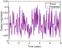
(a) HCRNN.

(b) HCRDNN 1.

(c) HCRDNN 2.

Fig. 5: Prediction capabilities of the proposed NN architectures.

VI-B MSE Performance

The MSE performance in the training and testing phases of the proposed NN architectures is depicted in Figs. 6 and 7, respectively, compared to the state-of-the-art NNs. The MSE is utilized to evaluate the average squared difference between the ground-truth and predicted SI signal modeled by the various NN architectures. As seen from the figures, the MSE values of all NNs are comparable in both training and testing phases (this can be clearly observed from the inset graphs in Figs. 6 and 7). As previously stated, the reason behind this is that all NNs are set to attain a comparable cancellation performance, and that is why they achieve a similar MSE performance. Moreover, it can be observed from Figs. 6 and 7 that there are no overfitting signs for the proposed and the state-of-the-art NNs as they perform well in both training and testing phases. Additionally, it can be seen from the figures that the proposed NNs converge to similar, low MSE values in both training and testing phases, which indicates the goodness of the solution provided by the proposed NN architectures.

VI-C Achieved SI Cancellation

The boxplots quantifying the total SI cancellation achieved by the proposed and the state-of-the-art NN-based canceler is depicted in Fig. 8. Here, we calculate the mean cancellation provided by the NN-based cancelers over the employed 15 network initializations. As seen from the figure, all NNs attain a comparable cancellation performance to the polynomial canceler at $P=5$ (red dashed-line in Fig. 8). Specifically, the mean cancellation achieved by all NN-based cancelers varies from 44.40 to 45.27 dB, which is very close to the polynomial target cancellation. It is worth noting that we configure the NN settings to achieve a comparable cancellation performance to the polynomial canceler as it is not easy to adjust the setting to exactly achieve the target cancellation.

Fig. 6: MSE in the training phase for the proposed and the state-of-the-art NN architectures.

Fig. 7: MSE in the testing phase for the proposed and the state-of-the-art NN architectures.

VI-D PSD Performance

In this subsection, we evaluate the PSD of the SI signal before applying any SI cancellation techniques (blue curve in Fig. 9). Further, the PSD of the residual SI signal after the linear cancellation process is assessed (red curve). Similarly, we depict the PSD of the SI signal after performing non-linear cancellation using the polynomial and NN-based cancelers. Finally, we show the PSD of the receiver background noise when there is no transmission, i.e., the receiver’s noise floor (black curve). As can be inferred from Fig. 9, the linear canceler provides 37.90 dB SI cancellation by bringing the SI signal’s power down from -42.74 dBm to -80.60 dBm. Moreover, the polynomial-based canceler attains an additional 6.6 dB cancellation by bringing the residual SI signal’s power down from -80.60 dBm to -87.19 dBm, making it very close to the receiver noise floor (approximately 3 dB above the receiver’s noise floor). A similar task is performed by the proposed and the state-of-the-art NN-based cancelers, in which they cancel the SI signal after the linear canceler by 6.55-7.40 dB, making it very akin to the receiver’s background noise level as illustrated in the inset graph of Fig. 9.

VI-E Computational Complexity and Memory Requirements

In this subsection, we assess the computational complexity of the proposed and the state-of-the-art NN-based cancelers in terms of the number of FLOPs and calculate the complexity reduction provided by each canceler compared to the polynomial canceler. Similarly, we quantify the memory requirements of each NN-based canceler in terms of the number of parameters and calculate the amount of reduction compared to the baseline canceler. The results of the comparison are graphically shown in Fig. 10 and numerically summarized in Table XI.

Fig. 8: Total SI cancellation of the proposed and the state-of-the-art NN-based cancelers.

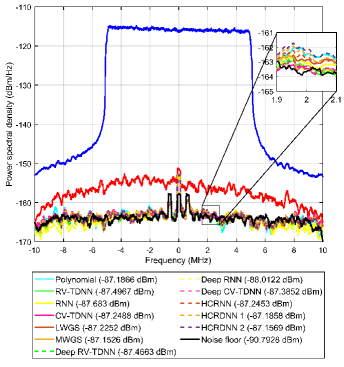
Fig. 9: PSD of the modeled SI signal using the proposed and the state-of-the-art NN-based cancelers.

VI-E1 Computational Complexity

Table XI illustrates the reduction in the number of FLOPs provided by the proposed HCRNN and HCRDNN-based cancelers compared to the polynomial and the state-of-the-art NN-based cancelers. As seen from Table XI, the proposed NN-based cancelers achieve a superior enhancement in the computational complexity compared to the polynomial-based canceler. For instance, the HCRNN provides a 52.18% reduction in the number of FLOPs while maintaining the same cancellation performance of the polynomial canceler. In addition, the HCRDNN 1 and HCRDNN 2 achieve 55.07% and 53.47% reduction compared to the polynomial canceler, respectively. However, the shallow and deep RV-TDNN, RNN, and CV-TDNN barely attain one half of the complexity reduction provided by the proposed NN architectures.

On the other hand, the proposed HCRNN, HCRDNN 1, and HCRDNN 2 architectures outperform the state-of-the-art MWGS by providing 18%, 20.92%, and 19.32% more reduction in FLOPs, respectively. Further, they attain 2.4%, 5.3%, and 3.7% more saving in FLOPs compared to the LWGS-based canceler, respectively. The above-mentioned results substantiate the proposed cancelers’ superiority in modeling the SI with low computational complexity compared to the polynomial and the state-of-the-art NN-based cancelers.

Fig. 10: Computational complexity and memory requirements of the proposed and the state-of-the-art NN-based cancelers.

VI-E2 Memory Requirements

Similarly, the reduction in the number of parameters of the proposed HCRNN and HCRDNN-based cancelers compared to the polynomial and the state-of-the-art NN-based cancelers is illustrated in Table XI. As can be observed, the shallow and deep structures of the RV-TDNN and RNN significantly increase the required parameters compared to the polynomial canceler. The former comes from dealing with the real and imaginary parts separately, while the latter results from employing a large number of feedback connections to efficiently detect the data sequences. On the other hand, the proposed HCRNN, HCRDNN 1, and HCRDNN 2 reduce the number of parameters by 26.60%, 20.51%, and 28.53% compared to the polynomial canceler, respectively. This reduction is due to the application of a convolutional layer before the recurrent layer in the proposed NN architectures, which mitigates the huge memory requirements of the recurrent layer. It can also be seen from Table XI that the reduction in parameters provided by the proposed NNs is comparable to that attained by the shallow and deep CV-TDNN. Further, the LWGS and MWGS provide the most reduction in the number of parameters.

However, the proposed NNs outperform the LWGS and MWGS in the number of FLOPs. More importantly, it can be inferred from Table XI that among all NN architectures, the proposed HCRDNN 1 attains the best reduction in FLOPs. Furthermore, the proposed HCRNN achieves the best compromise among the cancellation performance, number of FLOPs, and parameters. As such, the proposed NN-based cancelers offer high design flexibility for hardware implementation, depending on the system demands.

TABLE XI: Reduction in the number of FLOPs and parameters for the proposed and the state-of-the-art NN-based cancelers compared to the polynomial canceler with $P=5$.

Network	SI Canc. (dB)	Complexity		Complexity Reduction
		# Par.	# FLOPs	# Par.	# FLOPs
Polynomial ($P\negthinspace=$ 5)	44.45	312	1558	-	-
RV-TDNN	44.76	550	1156	+76.28%	-25.80%
RNN	44.94	528	1210	+69.23%	-22.34%
CV-TDNN	44.50	238	1166	-23.72%	-25.16%
LWGS	44.48	162	782	-48.08%	-49.81%
MWGS	44.40	212	1026	-32.05%	-34.15%
Deep RV-TDNN	44.73	538	1120	+72.44%	-28.11%
Deep RNN	45.27	1420	3106	+355.13%	+99.36%
Deep CV-TDNN	44.63	228	1106	-26.92%	-29.01%
HCRNN	44.50	229	745	-26.60%	-52.18%
HCRDNN 1	44.44	248	700	-20.51%	-55.07%
HCRDNN 2	44.41	223	725	-28.53%	-53.47%

VII Future Research Directions

In this work, the proposed NN architectures have been verified using a dataset that is captured by a single-input single-output FD test-bed. The joint design of multiple-input multiple-output (MIMO) and FD should be considered for B5G wireless networks [References]-[References], and the prospects of the proposed NNs could be generalized and verified using datasets captured by massive MIMO FD test-beds. Nevertheless, several challenges need to be solved prior to the deployment and design of such a system, which include but are not limited to the self- and cross-talks among the transceiver’s antennas [References]. Such challenges deserve a full investigation and will be studied in future work.

On the other hand, applying different machine learning techniques, such as support vector machines (SVM) [References], for SI cancellation in FD systems is identified as another future direction of investigation. Several challenges related to the high computational complexity of the SVM models can be considered in the future.

VIII Conclusion

In this paper, two hybrid-layers NN architectures, referred to as hybrid-convolutional recurrent NN (HCRNN) and hybrid-convolutional recurrent dense NN (HCRDNN), have been proposed for the first time to model the FD system SI with reduced computational complexity. The former exploits the weight sharing characteristics and dimensionality reduction potential of the convolutional layer to extract the memory effect and non-linearity incorporated into the input signal using a reduced network scale. Moreover, it employs the high modeling capabilities of the recurrent layer to help learn the temporal behavior of the input signal. The latter exploits an additional dense layer to build a deeper NN model with low complexity. The complexity analysis of the proposed NN architectures has been conducted, and the optimum settings for their training have been selected. Our findings demonstrate that the proposed HCRNN and HCRDNN-based cancelers attain a reduction in the computational complexity with 52% and 55% over the polynomial-based canceler, respectively, while maintaining the same cancellation performance. In addition, the proposed HCRNN and HCRDNN offer astounding complexity reduction over the shallow and deep NN-based cancelers in the literature.

Representation of Non-linear Systems using Polynomial-based Models

In the following, we review the common methods for representing non-linear systems using polynomial-based models (e.g., Hammerstein and parallel-Hammerstein), which are considered the cornerstone of approximating the SI in FD transceivers. Herein, it is assumed that all signals are of a narrow-band nature [References]. In addition, only the odd order non-linearities are considered since the even order non-linearities lay outside the passband [References] and are typically filtered by the BPFs in the FD transceiver [References].

-A Hammerstein Model

The Hammerstein model is one of the widely-known models for approximating the non-linear behavior with $M$-tap memory. In the Hammerstein model, a static non-linearity $N(.)$ is employed in series with a linear filter $L(.)$ in order to model the non-linearity with memory as follows [References]:

$$y(n)=L\left[N\left[x\left(n\right)\right]\right]=\sum_{m=0}^{M}h_{m}\sum_{\underset{p\,odd}{p=1,}}^{P}a_{p}\,x(n-m)\left|\,x(n-m)\right|^{p-1},$$ (46)

where $P$ indicates the order of non-linearity, whereas $h_{m}$ and $a_{p}$ represent the coefficients of the linear filter $L(.)$ and the non-linearity $N(.)$, respectively.

-B Parallel-Hammerstein (PH) Model

An extended version of the Hammerstein model is the PH model, which is constructed by combining the outputs of several Hammerstein models and can be identified as [References]:

$$y(n)=\sum_{\underset{p\,odd}{p=1,}}^{P}\sum_{m=0}^{M}h_{m,p}\,x(n-m)\left|x(n-m)\right|^{p-1},$$ (47)

where $h_{m,p}$ represent the coefficients of the linear filter corresponding to that order of non-linearity.

The PH model (47) can be rewritten as [References] as follows:

$$y(n)=\sum_{\underset{p\,odd}{p=1,}}^{P}\sum_{m=0}^{M}h_{m,p}\,x(n-m)^{\frac{p+1}{2}}x^{*}(n-m)^{\frac{p-1}{2}},$$ (48)

where $\left(.\right)^{*}$ indicates the complex conjugate operator. The PH model (48) provides a more general polynomial representation for approximating the non-linearity with memory and is considered the cornerstone of modeling the SI in FD transceivers.

References

- [1] M. Giordani, M. Polese, M. Mezzavilla, S. Rangan, and M. Zorzi, “Toward 6G networks: Use cases and technologies,” IEEE Commun. Mag., vol. 58, no. 3, pp. 55–61, Mar. 2020.
- [2] W. Saad, M. Bennis, and M. Chen, “A vision of 6G wireless systems: Applications, trends, technologies, and open research problems,” IEEE Netw., vol. 34, no. 3, pp. 134–142, May 2020.
- [3] H. V. Nguyen, V. Nguyen, O. A. Dobre, S. K. Sharma, S. Chatzinotas, B. Ottersten, and O. Shin, “On the spectral and energy efficiencies of full-duplex cell-free massive MIMO,” IEEE J. Sel. Areas Commun., vol. 38, no. 8, pp. 1698–1718, Jun. 2020.
- [4] A. Sabharwal, P. Schniter, D. Guo, D. W. Bliss, S. Rangarajan, and R. Wichman, “In-band full-duplex wireless: Challenges and opportunities,” IEEE J. Sel. Areas Commun., vol. 32, no. 9, pp. 1637–1652, Sept. 2014.
- [5] D. Kim, H. Lee, and D. Hong, “A survey of in-band full-duplex transmission: From the perspective of PHY and MAC layers,” IEEE Commun. Surveys Tuts., vol. 17, no. 4, pp. 2017–2046, Feb. 2015.
- [6] Z. Zhang, K. Long, A. V. Vasilakos, and L. Hanzo, “Full-duplex wireless communications: Challenges, solutions, and future research directions,” Proc. IEEE, vol. 104, no. 7, pp. 1369–1409, Jul. 2016.
- [7] K. E. Kolodziej, B. T. Perry, and J. S. Herd, “In-band full-duplex technology: Techniques and systems survey,” IEEE Trans. Microw. Theory Techn., vol. 67, no. 7, pp. 3025–3041, Jul. 2019.
- [8] M. Duarte, C. Dick, and A. Sabharwal, “Experiment-driven characterization of full-duplex wireless systems,” IEEE Trans. Wireless Commun., vol. 11, no. 12, pp. 4296–4307, Dec. 2012.
- [9] E. Everett, A. Sahai, and A. Sabharwal, “Passive self-interference suppression for full-duplex infrastructure nodes,” IEEE Trans. Wireless Commun., vol. 13, no. 2, pp. 680–694, Feb. 2014.
- [10] A. Balatsoukas-Stimming, P. Belanovic, K. Alexandris, and A. Burg, “On self-interference suppression methods for low-complexity full-duplex MIMO,” in Proc. Asilomar Conf. Signals, Syst. Comput., Nov. 2013, pp. 992–997.
- [11] M. Duarte and A. Sabharwal, “Full-duplex wireless communications using off-the-shelf radios: Feasibility and first results,” in Proc. 44th Asilomar Conf. Signals, Syst., Comput., Nov. 2010, pp. 1558–1562.
- [12] Y.-S. Choi and H. Shirani-Mehr, “Simultaneous transmission and reception: Algorithm, design and system level performance,” IEEE Trans. Wirel. Commun., vol. 12, no. 12, pp. 5992–6010, Dec. 2013.
- [13] B. Debaillie et al., “Analog/RF solutions enabling compact full-duplex radios,” IEEE J. Sel. Areas Commun., vol. 32, no. 9, pp. 1662–1673, Sep. 2014.
- [14] L. Laughlin, M. A. Beach, K. A. Morris, and J. L. Haine, “Optimum single antenna full duplex using hybrid junctions,” IEEE J. Sel. Areas Commun., vol. 32, no. 9, pp. 1653–1661, Sep. 2014.
- [15] E. Ahmed and A. M. Eltawil, “All-digital self-interference cancellation technique for full-duplex systems,” IEEE Trans. Wireless Commun., vol. 14, no. 7, pp. 3519–3532, Jul. 2015.
- [16] D. Korpi, L. Anttila, and M. Valkama, “Nonlinear self-interference cancellation in MIMO full-duplex transceivers under crosstalk,” EURASIP J. Wireless Commun. Netw., vol. 2017, no. 1, pp. 1–15, Dec. 2017.
- [17] T. O’Shea and J. Hoydis, “An introduction to deep learning for the physical layer,” IEEE Trans. Cogn. Commun. Netw., vol. 3, no. 4, pp. 563–575, Dec. 2017.
- [18] M. Gao, Y. Li, O. A. Dobre, and N. Al-Dhahir, “Joint blind identification of the number of transmit antennas and MIMO schemes using Gerschgorin radii and FNN,” IEEE Trans. Wireless Commun., vol. 18, no. 1, pp. 373–387, Jan. 2019.
- [19] H. Ye, G. Y. Li, and B.-H. F. Juang, “Power of deep learning for channel estimation and signal detection in OFDM systems,” IEEE Wireless Commun. Lett., vol. 7, no. 1, pp. 114–117, Feb. 2018.
- [20] H. He, C.-K. Wen, S. Jin, and G. Y. Li, “Deep learning-based channel estimation for beamspace mmWave massive MIMO systems,” IEEE Wireless Commun. Lett., vol. 7, no. 5, pp. 852–855, Oct. 2018.
- [21] X. Cheng, D. Liu, C. Wang, S. Yan, and Z. Zhu, “Deep learning-based channel estimation and equalization scheme for fbmc/oqam systems,” IEEE Wireless Commun. Lett., vol. 8, no. 3, pp. 881–884, Jun. 2019.
- [22] T. Gruber, S. Cammerer, J. Hoydis, and S. T. Brink, “On deep learning-based channel decoding,” in Proc. IEEE 51st Annu. Conf. Inf. Sci. Syst. (CISS), Baltimore, MD, USA, Mar. 2017, pp. 1–6.
- [23] T. Liu, S. Boumaiza, and F. M. Ghannouchi, “Dynamic behavioral modeling of 3G power amplifiers using real-valued time delay neural networks,” IEEE Trans. Microw. Theory Tech., vol. 52, no. 3, pp. 1025– 1033, Mar. 2004.
- [24] F. Mkadem and S. Boumaiza, “Physically inspired neural network model for RF power amplifier behavioral modeling and digital predistortion,” IEEE Trans. Microw. Theory Technol., vol. 59, no. 4, pp. 913–923, Apr. 2011.
- [25] Xin Hu et al., “Convolutional neural network for behavioral modeling and predistortion of wideband power amplifiers,” May 2020. [Online]. Available: https://arxiv.org/abs/2005.09848.
- [26] C. Tarver, L. Jiang, A. Sefidi, and J. Cavallaro, “Neural network DPD via backpropagation through a neural network model of the PA,” in Proc. 53rd Asilomar Conf. Signals, Syst., Comput., Nov. 2019, pp. 358–362.
- [27] R. Hongyo, Y. Egashira, T. M. Hone, and K. Yamaguchi, “Deep neural network-based digital predistorter for Doherty power amplifiers,” IEEE Microw. Wireless Compon. Lett., vol. 29, no. 2, pp. 146–148, Feb. 2019.
- [28] C. Häger and H. D. Pfister, “Nonlinear interference mitigation via deep neural networks,” in Proc. Opt. Fiber Commun. Conf. (OFC), San Diego, CA, USA, Mar. 2018, pp. 1–3.
- [29] A. Balatsoukas-Stimming, “Non-linear digital self-interference cancellation for in-band full-duplex radios using neural networks,” in Proc. IEEE Int. Workshop Signal Process. Adv. Wireless Commun. (SPAWC), Jun. 2018, pp. 1–5.
- [30] A. T. Kristensen, A. Burg, and A. Balatsoukas-Stimming, “Advanced machine learning techniques for self-interference cancellation in full-duplex radios,” in Proc. 53rd Asilomar Conf. Signals, Syst., Comput., Nov. 2019, pp. 1149–1153.
- [31] Y. Kurzo, A. Burg, and A. Balatsoukas-Stimming, “Design and implementation of a neural network aided self-interference cancellation scheme for full-duplex radios,” in Proc. 52nd Asilomar Conf. Signals, Syst., Comput., Oct. 2018, pp. 589–593.
- [32] Y. Kurzo, A. T. Kristensen, A. Burg, and A. Balatsoukas-Stimming, “Hardware implementation of neural self-interference cancellation,” IEEE J. Emerg. Sel. Topics Circuits Syst., vol. 10, no. 2, pp. 204-216, Jun. 2020.
- [33] M. Elsayed, A. A. A. El-Banna, O. A. Dobre, W. Shiu, and P. Wang, “Low complexity neural network structures for self-interference cancellation in full-duplex radio,” IEEE Commun. Lett., vol. 25, no. 1, pp. 181-185, Jan. 2021.
- [34] M. Isaksson, D. Wisell, and D. Ronnow, “A comparative analysis of behavioral models for RF power amplifiers,” IEEE Trans. Microw. Theory Tech., vol. 54, no. 1, pp. 348–359, Jan. 2006.
- [35] R. Zayani, R. Bouallegue, and D. Roviras, “Adaptive predistortions based on neural networks associated with levenberg-marquardt algorithm for satellite down links,” EURASIP J. Wireless Commun. Net., vol. 2008, no. 1, p. 2, Jul. 2008.
- [36] J. X. Peng, K. Li, and D. S. Huang, “A hybrid forward algorithm for RBF neural network construction,” IEEE Trans. Neural Netw., vol. 17, no. 6, pp. 1439–1451, Nov. 2006.
- [37] X. Xia, K. Xu, D. Zhang, Y. Xu, and Y. Wang, “Beam-domain full-duplex massive MIMO: Realizing co-time co-frequency uplink and downlink transmission in the cellular system,” IEEE Trans. Veh. Technol., vol. 66, no. 10, pp. 8845–8862, Oct. 2017.
- [38] K. Xu, Z. Shen, Y. Wang, X. Xia, and D. Zhang, “Hybrid time-switching and power splitting SWIPT for full-duplex massive MIMO systems: A beam-domain approach,” IEEE Trans. Veh. Technol., vol. 67, no. 8, pp. 7257–7274, Aug. 2018.
- [39] X. Xia, K. Xu, Y. Wang, and Y. Xu, “A 5G-enabling technology: Benefits, feasibility, and limitations of in-band full-duplex mmimo,” IEEE Veh. Technol. Mag., vol. 13, no. 3, pp. 81–90, Sep. 2018.
- [40] C. Auer, K. Kostoglou, T. Paireder, O. Ploder, and M. Huemer, “Support vector machines for self-interference cancellation in mobile communication transceivers,” in Proc. IEEE Veh. Technol. Conf. (VTC-Spring), 2020, pp. 1–6.