Identification of the invariant manifolds of the LiCN molecule using Lagrangian descriptors

Abstract

In this paper, we apply Lagrangian descriptors to study the invariant manifolds that emerge from the top of two barriers existing in the LiCN$\rightleftharpoons$LiNC isomerization reaction. We demonstrate that the integration times must be large enough compared with the characteristic stability exponents of the periodic orbit under study. The invariant manifolds manifest as singularities in the Lagrangian descriptors. Furthermore, we develop an equivalent potential energy surface with 2 degrees of freedom, which reproduces with a great accuracy previous results [Phys. Rev. E 99, 032221 (2019)]. This surface allows the use of an adiabatic approximation to develop a more simplified potential energy with solely 1 degree of freedom. The reduced dimensional model is still able to qualitatively describe the results observed with the original 2-degrees-of-freedom potential energy landscape. Likewise, it is also used to study in a more simple manner the influence on the Lagrangian descriptors of a bifurcation, where some of the previous invariant manifolds emerge, even before it takes place.

I Introduction

Molecular systems usually exhibit a very rich and intricate dynamics, even in small molecules formed solely by a few atoms [1], due to nonlinear interactions [2]. The existence of conical intersections [3, 4] between Born-Oppenheimer potential energy surfaces (PES) adds additional complexity to the classical characterization of these systems, as molecules may undergo electronic transitions in their neighborhoods [5]. Likewise, the combination of these effects easily opens effective routes to chaos, making the analysis of the corresponding dynamics more complex, in particular when bifurcations take place and substantially modify the structure of the phase space.

Suitable tools to cope with the previous problems can be borrowed from dynamical systems theory [6], which sets up the molecular phase space as the proper arena for a dynamical analysis. Accordingly, for low excitation energies the motion of the nuclei takes place in the vicinity of the lowest equilibrium point of the PES, where the harmonic approximation is valid and the motions are well characterized by the normal modes [1]. The structure of the corresponding phase space is mostly regular, with all motions organized in invariant tori. As the excitation energy increases, the anharmonicities and the coupling among the different modes open the door to irregular motion and effective intramolecular vibrational relaxation [7]. From a nonlinear dynamics perspective, these phenomena can be partially explained through the Kolmogorov-Arnold-Moser theorem [8], which dictates that the perturbation associated with the energy growth destroys some of the previous tori. In addition, the Poincaré-Birkhoff theorem [9] locally controls the vicinity of the regions where resonances among modes are important [5]. Eventually, the vibrational energy can become large enough to classically overcome energetic barriers (typically saddles) in the PES; this gives rise to chemical reactivity [10].

The study of chemical reactions from a dynamical perspective dates back to Marcelin’s [11] and Wigner’s [12] pioneering works on transition state theory [13], which are also applicable to other physical processes in which the system can be partitioned into different regions [14, 15, 16, 17]. The key point is the study of the dynamics at the top of the barrier separating two such parts (usually referred to as the reactants and the products), where some relevant geometrical structures can be identified, i.e., a normally hyperbolic invariant manifold [16] and its invariant manifolds [18], which locally determine the classical reactive dynamics. Moreover, at the quantum level, tunneling and interference might be important [19, 20, 21, 22]. Early examples of classical structures in two-dimensional problems were envisioned, for example, in Ref. 23. These concepts have also been generalized to the case of noisy driven systems, [24, 25, 26, 27, 28, 29], using a chaotic trajectory that jiggles around the barrier top stochastically. Based on these theories, many studies to understand chemical reactivity have been conducted considering only the barrier top on the PES, since this is the most important dynamical bottleneck. However, other phase-space dynamical barriers [30, 31, 32, 33] may exist interfering with the motion in this region, and modulating, for example, the corresponding time scales [34]. The correct identification of the geometrical structures, i. e., the invariant manifolds, in this other situation is similarly of great importance.

The aim of this paper is the identification of the invariant manifolds that emerge from the top of two barriers existing in the LiCN$\rightleftharpoons$LiNC isomerization reaction, paying special attention to those of dynamical origin. These manifolds act as true geometrical separatrices for the system. For this purpose, we use the Lagrangian descriptors (LDs) [35, 36], a recently developed tool that allows the study of the classical flow of dynamical systems in a very simple and effective way.

First, we introduce an alternative PES with 2 degrees of freedom (dof) that is formed by Morse potentials. We demonstrate that the results obtained using this PES are in excellent agreement with those yielded by the original ab initio one, even when a constant moment of inertia is considered (see discussion in Sec. IV.2).

Second, in order to avoid the complicated picture derived from excessive homoclinic and heteroclinic intersections, in the previous PESs, which have 2 dof we make use of the adiabatic approximation in order to obtain an equivalent 1-dof model, something that is feasible due to the great performance of PES formed by Morse oscillators. The reduced dimensional model is nevertheless able to capture the phenomenology that takes place in the vicinity of the barriers existing in the system and, as a consequence, provides an adequate characterization of its dynamics (see Sec. IV.3).

This paper is organized as follows. After the Introduction, we present in Sec. II the system under study, highlighting the main dynamical peculiarities and four periodic orbits (POs) that are relevant for our work. Section III briefly describes the method used to unveil the structures existing in the vibrational phase space of our system. Next, we present in Sec. IV the main results of our work, paying special attention to the geometry surrounding the dynamical barrier, along with the corresponding discussion. Finally, we conclude the paper in Sec. V with the Summary and Outlook.

II System and classical trajectories

In this section we report the main properties of the isomerizing reaction under study. To begin, we present in Sec. II.1 the Hamiltonian function that models the system. Next, in Sec. II.2, we describe an alternative PES formed by a collection of Morse oscillators. obtained by making use of an adiabatic approximation. Finally, Sec. II.3 is devoted to a brief description of the vibrational dynamics of the studied molecule.

II.1 Hamiltonian model with 2 degrees of freedom

The system under study is the rotationless ($J=0$) triatomic LiCN molecule. Here, the motion associated with the triple bond in the C$\equiv$N fragment has a very high frequency, and consequently decouples from the rest of the molecular modes. Accordingly, the CN stretch dof can be assumed to remain constant at its equilibrium value, $r_{\rm eq}=2.186$ a.u. The vibrations of the LiCN can then be very well described with the following 2-dof Hamiltonian:

$$\mathcal{H}_{2}=\frac{P_{R}^{2}}{2\mu_{1}}+\frac{P_{\vartheta}^{2}}{2}\left(\frac{1}{\mu_{1}R^{2}}+\frac{1}{\mu_{2}r_{\rm eq}^{2}}\right)+V_{\rm{a.i.}}(R,\vartheta),$$ (1)

where the distance $R$ and the angle $\vartheta$ determine the position of the Li atom with respect to the center of mass of C-N, $\mu_{1}=m_{\rm Li}(m_{\rm C}+m_{\rm N})/(m_{\rm Li}+m_{\rm C}+m_{\rm N})$, and $\mu_{2}=(m_{\rm C}m_{\rm N})/(m_{\rm C}+m_{\rm N})$ are reduced masses, and $V_{\rm{a.i.}}(R,\vartheta)$ is the ab initio PES [37], which is shown in Fig. 1 in the form of a contours plot. As can be seen, this PES has two stable minima (green squares), which correspond to the two stable isomers at the collinear configurations Li-CN ($\vartheta=0$ rad, with an energy of 2281 cm^-1) and CN-Li ($\vartheta=\pi$ rad, with an energy of 0 cm^-1). These two minima are separated by a modest energetic barrier for the isomerization along the minimum energy path (MEP) given by $R_{\text{MEP}}(\vartheta)$ (dashed green line), whose top has an energy of $E_{\text{SP}}=3455$ cm^-1 and a saddle$\times$center structure in the phase space (index-1 saddle, shown as a cross).

In the next section, we report a simplified PES, which is still able to reproduce the main characteristics of the ab initio PES introduced in Fig. 1.

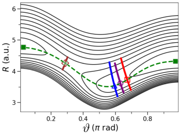
Figure 1: Ab initio potential energy surface for LiCN molecule with 2 degrees of freedom. It has two minima (green squares) corresponding to the (stable) linear configurations Li-C$\equiv$N ($\vartheta=0$ rad) and C$\equiv$N-Li ($\vartheta=\pi$ rad), which are connected by the minimum energy path (dashed green line) for the isomerization reaction, which passes through a rank-1 saddle (green cross contained in the brown diamond). Four periodic orbits relevant to our work are also shown. The remaining symbols highlight the intersection of the previous trajectories with the minimum energy path; this defines the Poincaré surface of section, where initial conditions are taken (see text for details).

II.2 Equivalent potential energy surface with 2 degrees of freedom

As can be seen, for constant $\vartheta$, the ab initio PES shown in Fig. 1 increases abruptly for small $R$ while it is a slow varying function for large $R$. This behavior is well described by

$$V_{\rm equiv}(R,\vartheta)=V_{\rm MEP}(\vartheta)+V_{\rm Morse}(R,\vartheta),$$ (2)

where $V_{\rm MEP}(\vartheta)=V_{\rm{a.i.}}(R_{\rm MEP}(\vartheta),\vartheta)$ is the potential along the MEP, and

$$V_{\rm Morse}(R,\vartheta)=D(\vartheta)\left[1-e^{-\alpha(\vartheta)(R-R_{\rm min})}\right]^{2}$$ (3)

is the Morse potential, which depends on the distance $R$ and also on the angular coordinate, $\vartheta$, through the well depth $D(\vartheta)$ and the width $\alpha(\vartheta)$. This width is usually expressed as a function of the frequency $\Omega(\vartheta)$ as $\alpha(\vartheta)=\sqrt{\Omega(\vartheta)\mu_{1}/(2D(\vartheta))}$. Consequently, a different Morse potential is used for each $\vartheta$.

In order to be able to use the potential (3) efficiently, we have performed an additional fitting of the functions $D(\vartheta)$ and $\Omega(\vartheta)$ as

$$D(\vartheta) = \sum_{n=0}^{9}d_{n}\cos(n\vartheta),$$ (4)

$$\Omega(\vartheta) = \sum_{n=0}^{9}w_{n}\cos(n\vartheta).$$ (5)

The fitted coefficients $d_{n}$ and $w_{n}$ are listed in Table 1. We have verified that the error in Eqs. (4) and (5) with respect to their original expressions is in all cases less than 0.3%, which provides an estimation of the difference between the potential (2) and the original ab initio potential. Figure 2 shows the values of $D(\vartheta)$ and $\Omega(\vartheta)$ obtained for the system under study. As can be seen, both functions have two maxima at $\vartheta=0,\pi$ rad, and a minimum in between (found at $\vartheta\sim 0.30\pi$ and $0.44\pi$ rad, respectively).

In the next section we briefly summarize the vibrational dynamics for Hamiltonian (1). Let us remark that the results reported there, which are associated with the ab initio PES, are also quantitatively valid for the adiabatically obtained PES (2) due to their high similarity.

Table 1: Fitted coefficients $d_{n}(\pm\,3\times 10^{-7}$ a.u.) and $w_{n}(\pm\,5\times 10^{-8}$ a.u.) of Eqs. (4) and (5), respectively.

$n$	$d_{n}$(10-4 a.u.)	$w_{n}$ (10-5 a.u.)
0	$2362.990$	$303.267$
1	$-67.946$	$-21.217$
2	$17.920$	$36.838$
3	$17.416$	$11.288$
4	$14.756$	$-2.689$
5	$-1.468$	$-7.388$
6	$4.181$	$4.693$
7	$0.845$	$2.215$
8	$1.290$	$-0.616$
9	$0.054$	$-1.144$

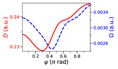
Figure 2: Parameters of the Morse potential: trap depth (4) (continuous red line), and frequency (5) (dashed blue line).

II.3 Trajectories and vibrational dynamics

The dynamics of this system is followed by computation of classical trajectories $(R,\vartheta,P_{R},P_{\vartheta})$ which evolve in the four-dimensional phase space as Hamiltonian (1) has 2 dof. In practice, all initial conditions are taken on an adequate Poincaré surface of section (PSOS) [6]. In this case, such a suitable PSOS is choosen along the MEP, which renders the most relevant dynamical information, i.e., that concerning the angular motion. As the MEP is not an actual trajectory of LiCN, and in order to make the PSOS an area preserving map, a transformation to new coordinates must be performed [38, 31, 39]

$$\psi = \vartheta,\qquad\qquad\qquad\;P_{\psi}=P_{\vartheta}-\left(\frac{dR_{\text{MEP}}}{d\vartheta}\right)_{\vartheta=\psi}P_{R}$$

$$\rho = R-R_{\text{MEP}}(\vartheta),\quad P_{\rho}=P_{R}.$$ (6)

In Fig. 1, we also plot superimposed four POs which are relevant for this work. In particular, the purple one (second one starting from the right) is marginally stable, running almost vertically. This orbit emerges “out of the blue”‘ in a tangent or saddle-node bifurcation [31, 32] (SNB) $SN_{1}$ at $E_{SN_{1}}=3440.6$ cm^-1 (just below the energy $E_{\text{SP}}$, which must be exceeded in order to permit the isomerization). Subsequently, as energy increases this PO bifurcates in a pair, the one that moves leftwards being stable and the one moving rightwards being unstable. The result is shown in Fig. 1 for $E=4000$ cm^-1 in blue and red colors, respectively. The corresponding manifolds and their foldings and intersections [40] are very intricate, as shown in Fig. 3. Hereafter, we refer to the unstable PO as SN${}_{\textnormal{u}}$-PO. Other bifurcations in this molecule [41, 42] and other systems [43, 44] have been similarly reported.

Let us conclude this section by remarking that SNBs are also important quantum mechanically, since they can give rise to the so-called superscars, ith the result that some wave functions are strongly localized along the bifurcated POs. This phenomenon, first studied in a quantum map [45], has also been described in the molecule under study [32, 46]. The imprint of SNBs on spectral properties has also been considered by other authors [47, 48].

Finally, we also show in Fig. 1 the leftmost (brown) PO, which is a non-recrossing dividing surface [23]. We refer to this PO as TS-PO as it lies close to the position where the transition state or activated complex is formed [23, 49, 50]. It first appears at the saddle-point energy $E_{\text{SP}}$.

III Lagrangian descriptors

In order to unveil the phase space structures existing in our system in connection with the POs described in Sec. II, we use the LD computed as [51, 36, 40]

$$M(\mathbf{z}_{0},\tau)=\int_{-\tau}^{\tau}\sum_{i=1}^{4}|z_{i}(t)|^{p}\,dt,$$ (7)

where $\mathbf{z}_{0}=\left(\psi_{0},R_{0}=R_{\text{MEP}}(\psi_{0}),P_{\psi,0},P_{\rho,0}=0\right)$ is a vector of initial conditions taken in the PSOS defined in Eq. (6), $p$ a parameter defining the chosen norm, and $\tau$ a parameter defining the time interval in which the LD is calculated. Notice that the propagation of the trajectory is done forward and backward in order to capture the effects in the phase space of the unstable and stable manifolds at the same time. Some results for Hamiltonian (1) are shown in Fig. 3, both below and above the SNB energy, for $p=0.4$ and $\tau=2\times 10^{4}$ a.u. [40], this last integration time being 1 order of magnitude larger than the periods of the POs of interest shown in Fig. 1. We have also highlighted with different symbols the fixed points associated with those POs. As can be seen, the phase space is formed by a very complex structure due to the homoclinic intersections of the invariant manifolds, which become visible where the value of the LDs changes abruptly from a large value (shown in dark blue) to a small one (in yellow). These manifolds are identified as singularities in the LD plots, as is discussed later in more detail in Sec. IV. Notice also the existence of a region where the LDs are smooth functions, where they remain almost constant; this region is associated with the stability island that surrounds the stable PO, marked as a blue triangle. Note in this respect that LDs can also be used to characterize invariant tori [52] and the repeller in open systems [53]. The structure of the LDs in the whole phase space at these energies is shown in Fig. A.1 in Appendix A.

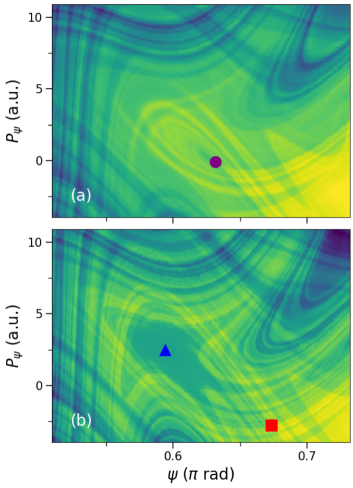
Figure 3: Lagrangian descriptors as defined in Eq. (7) with $p=0.4$, and $\tau=2\times 10^{4}$ a.u. computed from trajectories of LiCN for (a) $E=E_{\rm SN_{1}}=3440.6$ cm^-1, and for (b) $E=4000$ cm^-1. The purple circle, blue triangle and red square indicate the position of the parabolic, elliptic and hyperbolic points associated with the three rightmost periodic orbits shown in Fig. 1, which emerge due to a saddle-node bifurcation at $E=E_{\rm SN_{1}}$.

Due to the complexity of the geometrical objects in Fig. 3, we consider in the next section the results yielded by two simplified, yet equivalent, models. Both models are constructed using Morse potentials. The first one is that previously reported in Sec. II.2; it has 2 dof and reproduces the characteristics of Eq. (1) in the vicinity of the SNB with great precision. The second one has only 1 dof and was originally introduced in Ref. 31. This reduced dimensional model is still able to qualitatively reproduce the phase-space structures associated with Eq. (1) but not the heteroclinic intersections that occur when the invariant manifolds associated with different POs intersect.

IV Results and discussion

In this section we present our results and the corresponding discussion. This section is divided in three parts. First, we discuss in Sec. IV.1 the influence of the integration time on the LDs, showing that the invariant manifolds associated with a particular PO require a computation time large enough compared to the inverse of its characteristic exponents. Second, as an intermediate step towards the 1-dof equivalent model, we demonstrate the excellent performance of the equivalent adiabatic PES given by Eq. (2). Third, we conclude this section by studying the reduced dimensional model based on the adiabatic approximation, which is, nevertheless, capable of reproducing the main structures that determine the dynamics of the molecule.

IV.1 Influence of the integration time

Lagrangian descriptors are able to unravel invariant manifolds in phase space only if the integration time $\tau$ appearing in Eq. (7) is sufficiently large to account for their particular hyperbolic behavior.

The exponential sensitivity of an initial condition found in the neighborhood of a given unstable PO becomes manifest on a characteristic time scale given by the inverse of the stability exponents of its corresponding invariant manifolds. For systems with 2 dof, there are two of such exponents, $\lambda_{s,u}$, each one associated with the stable and the unstable manifold, respectively; the associated eigenvalues of the monodromy matrix are given by $\gamma_{s,u}=e^{\lambda_{s,u}T}$, where $T$ is the period and, as $\lambda_{u}=-\lambda_{s}\geq 0$, $\gamma_{s}\gamma_{u}=1$. In general, a neighboring trajectory will move apart from the reference PO at a rate given by $\sim$ $e^{\lambda_{u}t}$ in the direction of the unstable manifold. Conversely, it will approximate the PO in the direction of the stable manifold at a rate given by $\sim$ $e^{\lambda_{s}t}$ (or separate from it at the same rate when evolving backwards in time). Consequently, the particular character of the manifolds is expected to show up only for $|\tau|\geq|\lambda_{u,s}^{-1}|$.

In this work, we are mostly interested in the invariant manifolds associated with the unstable (left brown) TS-PO and (right red) SN${}_{\textnormal{u}}$-PO presented in Fig. 1, which are responsible for the formation barriers that obstruct isomerization. These two POs have different stability exponents, as can be seen in Fig. 4, where the inverse of their unstable exponent is shown. Notice that in both cases, $\lambda_{u}^{-1}$ reduces with the energy, though in the case of the SN${}_{\textnormal{u}}$-PO this happens in a much more dramatic way, especially at small energies. Actually, $\lambda_{{\rm SN}u-{\rm PO},u}^{-1}$ diverges at $E=E_{\rm SN_{1}}=3440.6$ cm^-1, since at the bifurcation this unstable PO collapses with the (blue) stable PO, rendering the (purple) marginally stable PO, whose monodromy matrix has two eigenvalues equal to 1, so its characteristic exponents must cancel (and then $\lambda_{u,s}^{-1}\rightarrow\pm\infty$).

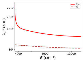
Figure 4: Inverse of the unstable stability exponent as a function of the energy. The top red (bottom brown) curve corresponds to the unstable periodic orbit (transition state trajectory) shown with the same coloring in Fig. 1.

Figures 5 and 6 show the value of the LDs as defined in Eq. (7) for different characteristic times $\tau=C\lambda_{u}^{-1}$ as a function of the stability exponent of the TS-PO and the SN${}_{\textnormal{u}}$-PO, respectively. As in Fig. 3, dark blue (yellow) coloring indicates a large (small) value in the LDs. Note that for the used energy of $E=4000$ cm^-1 the stability exponent for the TS-PO is almost two times larger than that of the SN${}_{\textnormal{u}}$-PO. Consequently, the integration times chosen in Fig. 5 are approximately half of those used in Fig. 6. This is the reason why Fig. 6 has a more detailed structure than Fig. 5.

When the integration time is small [by taking, for example, $\tau=\lambda_{u}^{-1}$, as done in Figs. 5(a) and 6(a)], the LD-plots show up as a blurry picture. Nonetheless, the results for Fig. 6(a) start to unveil the structure around the TS-PO, contrary to what happens in Fig. 5(a), where the integration time is still too small. Then, larger integration times are required to allow the identification of these invariant manifolds. Notice in particular the situation shown in Fig. 5(b), where $\tau=5\,\lambda_{{\rm TS-PO},u}^{-1}$. There, the manifolds emanating from the TS-PO are clearly visible, but not those associated with the SN${}_{\textnormal{u}}$-PO, because the characteristic exponent for this PO is smaller than for the previous one, and then longer times are required to study its behavior. The stability island that lies close to this trajectory in nevertheless visible. The manifolds for the SN${}_{\textnormal{u}}$-PO can be seen for a larger integration time such as $\tau=5\,\lambda_{{\rm SN_{\textnormal{u}}-PO},u}^{-1}$ as inferred by inspection of Fig. 6(b).

To conclude, we show in Figs. 5(c) and 6(c) the results for an integration time that is $\tau=10\,\lambda_{u}^{-1}$. In both cases, but especially in the second one, a very detailed picture of the chaotic region of phase space is obtained, where the complex structure of the heteroclinic tangle becomes visible. Thus, in the rest of the article integration times equal to $\tau=2\times 10^{4}$ a.u. will be used, a value that is slightly smaller than that considered in Fig. 6(c). Similar results are obtained for other comparable integration times as long as they are large enough compared to $\lambda_{u}^{-1}$. Let us conclude by pointing out that this criterion is not applicable to marginally stable POs (as it happens for the SN${}_{\textnormal{u}}$-PO at $E=E_{\rm SN_{1}}$), since then $\lambda_{u,s}=0$, and, as a consequence, $\lambda_{u,s}\rightarrow\pm\infty$.

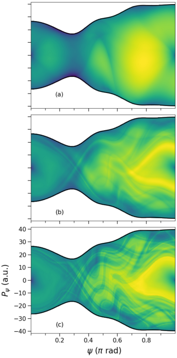
Figure 5: Lagrangian descriptors as defined in Eq. (7) computed from trajectories of LiCN for $E=4000$ cm^-1, $p=0.4$, and $\tau=C\lambda_{u}^{-1}$, $\lambda_{\textnormal{TS-PO},u}^{-1}\simeq 1163$ a.u. being the inverse of the stability exponent of the TS trajectory shown in brown in Fig. 1, and $C=1$ (a), 5 (b), and 10 (c), respectively.

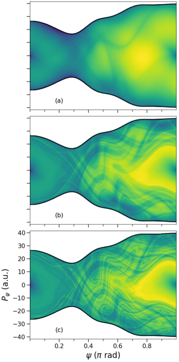
Figure 6: Same as Fig. 5 for the SN${}_{\textnormal{u}}$ trajectory shown in red in Fig. 1, whose stability exponent has an inverse equal to $\lambda_{\textnormal{SN}_{\textnormal{u}}-\textnormal{PO},u}^{-1}\simeq 2170$ a.u. at the energy of $E=4000$ cm^-1.

IV.2 Equivalent model with 2 degrees of freedom

In this section we discuss the excellent performance of the alternative PES given by Eq. (2). As the original ab initio PES, the new one has 2 dof so the system dynamics takes place in a 4-dimensional phase space. This study is conducted as a necessary intermediate step in order to to develop the reduced dimensional model reported in Sec. IV.3.

Figure 7 shows the value of the LDs in the vicinity of the SN bifurcation for the same set of parameters as those previously used in Fig. 3 but modelling the PES with Eq. (2). As can be seen, the structure that is observed using any of the two PESs is similar, both below [(a) panels] and above [(b) panels] the bifurcation energy $E_{\rm SN_{1}}$. Notice that the results shown in Figs. 3 and 7 have been obtained with the Hamiltonian (1), which has a moment of inertia associated with the angular coordinate, $\mathcal{I}_{\vartheta}=[1/(\mu_{1}R^{2})+1/(\mu_{2}r_{\rm eq}^{2})]^{-1}$, that is $R$-dependent. As a further simplification, one can take this moment of inertia as constant by setting it, e. g., equal to its value at the top of the largest energetic barrier, $\mathcal{I}_{\rm SP}=[1/(\mu_{1}R_{\rm MEP}^{2}(\vartheta_{\rm SP}))+1/(\mu_{2}r_{\rm eq}^{2})]^{-1}\simeq 4\times 10^{4}$ amu. As shown in Fig. 8(a), the structure of the phase space is almost equal to those already presented in Figs. 3(a) and 7(a), while above the bifurcation energy only minor differences are visible, as inferred by comparison of Figs. 3(b), 7(b), and 8(b).

The agreement between the results for the ab initio PES and those associated with the Morse-based PES allows us to make a further simplification in order to define a new model with only 1 dof, as discussed in the next section.

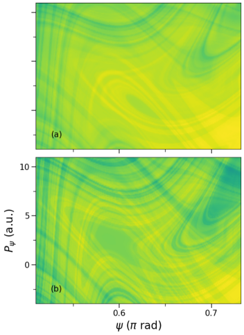
Figure 7: Same as Fig. 3 for the equivalent two-dimensional potential energy surface constructed using the adiabatic Morse potential. In both case, the exact moment of inertia $\mathcal{I}_{\vartheta}=[1/(\mu_{1}R^{2})+1/(\mu_{2}r_{\rm eq}^{2})]^{-1}$ is used.

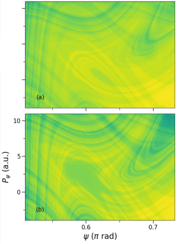
Figure 8: Same as Fig. 7 for a constant moment of inertia $\mathcal{I}_{\rm SP}=[1/(\mu_{1}R_{\rm MEP}^{2}(\vartheta_{\rm SP}))+1/(\mu_{2}r_{\rm eq}^{2})]^{-1}\simeq 3.94\times 10^{4}$ amu.

IV.3 Equivalent model with 1 degree of freedom

All POs shown in Fig. 1 correspond to almost pure vibrational stretching states, where the distance between the Li atom and the CN fragment changes periodically, while the angle $\vartheta$ remains almost constant. In this situation an adiabatic separation between the two modes can be carried out with good approximation, and then we neglect the stretching motion. Accordingly, Hamiltonian (1) can be substituted by the following 1-dof expression

$$\mathcal{H}_{1}=\frac{P_{\psi}^{2}}{2\mathcal{I}_{\psi}}+V_{\text{eff}}(\psi),$$ (8)

where $(P_{\psi},\psi)$ are now the (two-dimensional) phase-space coordinates; $\mathcal{I}_{\psi}$ is the moment of inertia associated with the coordinate $\psi$, which will be taken equal to its value at the saddle point located at the energy barrier top, i.e., $I_{\psi}=I_{\rm SP}$; and $V_{\text{eff}}$ is an effective potential for $\psi$. The accuracy of this model has been also assessed in previous works [49, 50, 54]. In this section, we demonstrate in detail its ability to adequately reproduce the invariant manifolds associated with the TS-PO and SN${}_{\textnormal{u}}$-POs. The section is divided in three parts. First, we introduce the potential energy considered in this case, which depends solely on the angle $\psi$. Second, Sec. IV.3.2 is devoted to the analysis of the existing manifolds below the bifurcation energy $E_{\rm SN_{1}}$, where the SN${}_{\textnormal{u}}$-PO appears. Third, we conclude in Sec. IV.3.3 by discussing the situation where the energy is larger than $E_{\rm SN_{1}}$.

IV.3.1 Potential energy

The simplest approximation for $V_{\text{eff}}$ in Eq. (8) is simply given by the potential energy along the MEP, $V_{\text{MEP}}(\psi)$, shown as a dashed green line in Fig. 1. This function is shown in the bottom dashed green line of Fig. 9. As can be seen, it reproduces qualitatively the same characteristics of the 2-dof PES $V_{\rm{a.i.}}(R,\vartheta)$, namely, two minima at $\psi=0$ and $\pi$ rad separated by a single maximum located at the barrier top $\psi=0.29\pi$ rad.

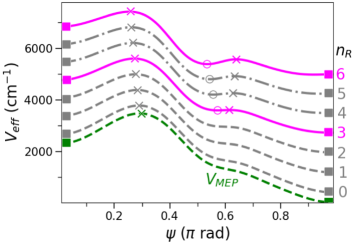
Figure 9: Effective potential with one degree of freedom along the angular coordinate for the LiCN molecule. The bottom dashed green line corresponds to the energy profile along the minimum energy path, $V_{\text{MEP}}(\psi)$, of the potential energy surface shown in Fig. 1. The remaining curves are the adiabatic potentials given by Eq. (9) for the $n_{R}$ values shown on the right. The positions of the minima potential wells’, local minima, and local maxima have been highlighted with squares, circles, and crosses, respectively.

The model described by Eq. (8) is not able to account for the emergence of the stable region shown in Fig. 3(b) for $V_{\text{eff}}(\psi)=V_{\rm MEP}(\psi)$ (see discussion in Sec. IV.3.2). As discussed in Ref. 31, this stabilization can be explained using an effective potential that is valid when the motion in the $R$ radius is much faster than that in the $\vartheta$, i. e., $\psi$, angle, just like in the stretching POs visible in the rightmost part of Fig. 1. Then, one can quantize the potential $V_{\rm equiv}(R,\vartheta)$ (2) for each value of the angle, to define a new 1-dof potential energy as

$$V_{\rm eff}(\psi) = V_{\rm MEP}(\psi)+\hbar\Omega(\psi)\left(n_{R}+\frac{1}{2}\right)$$ (9)

$$- \frac{\hbar^{2}\Omega^{2}(\psi)}{4D(\psi)}\left(n_{R}+\frac{1}{2}\right)^{2},$$

where $n_{R}$ is the corresponding vibrational excitation number, and $D=D(\psi)$ and $\Omega=\Omega(\psi)$ are the Morse parameters given by Eqs. (4) and (5), which depend on the angle $\psi$.

The effective potential (9) is shown in Fig. 9 for $n_{R}=0-6$. The potentials for $n_{R}=0,1$, and 2 (dashed gray lines) are very similar to that for the MEP. Consequently, the phase space presents qualitatively the same structure, as can be seen in Figs. B.1-B.3 in Appendix B. Notice, however, that the potential is flatter for $n_{R}=2$ than for $n_{R}=0$ around $\psi\simeq 0.6\pi$ rad. Furthermore, for $n_{R}>2$ the potential starts to show a minimum around that point, which is precisely responsible of the stabilization process previously described in the discussion of Fig. 1.

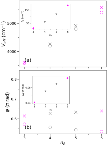
Figure 10: Characteristic parameters of the effective potential (9) shown in Fig. 9. (a) The top crosses and empty circles show, respectively, the potential energy at the local maximum (saddle point in phase space) and at the local minimum (center) of the dynamical barrier in the LiCN molecule as a function of the vibrational number $n_{R}$. The inset shows the height of the energetic barrier that is formed as the difference of the results of the main panel. (b) Position of the local maximum (crosses) and of the local minimum (empty circles) for the dynamical barrier. The inset shows the distance between the previous points.

Figure 10 shows some characteristic parameters of the effective potential (9). Firstly, Fig. 10(a) shows the value of the potential at the local maximum (saddle point) and at the local minimum (center) for the dynamical barrier. As can be seen, the potential energy increases with $n_{R}$ for all the previous points. However, the value of the potential at the saddle point increases faster than at the center, and, as a consequence, the energetic barrier height increases, as shown in the inset. For example, the energetic barrier is only 14 cm^-1 in height for $n_{R}=3$, while it equals 187 cm^-1 for $n_{R}=6$. Secondly, we show in Fig. 10(b) the positions of the critical points of the previous barrier. As can be seen in the corresponding inset, the distance between the saddle points and the centers increases with $n_{R}$, and then so does the width of the stability regions that show up.

To conclude, let us indicate that an alternative adiabatic approximation was obtained by Light and Bačić in Ref. [55], but was meant for a different purpose. There, the authors were interested in the development of an optimal basis set for the computation of the system eigenfunctions. No differences should be expected at the quantum level (eigenenergies, eigenfunctions, Husimi distributions, …) when comparing their results with those derived from our adiabatic PES with 2 dof. Nevetherless, their reduced dimensional potential energy functions with 1 dof do not present any relative minimum (see Fig. 3 of Ref. [55]) able to reproduce the SN bifurcation that is observed for the system with 2 dof, which has a strong classical imprint and a quantum imprint on the system [31, 32, 33].

IV.3.2 Phase-space geometry below the bifurcation energy $E_{SN_{1}}$

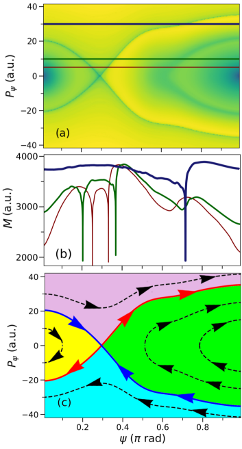
Figure 11: Phase space for the 1-degree-of-freedom model of LiCN (8) with $V_{\text{eff}}(\psi)=V_{\text{MEP}}(\vartheta)$. (a) Lagrangian descriptor as defined in Eq. (7). (b) The sections of constant $P_{\psi}=5,10,$ and 30 a.u. of the Lagrangian descriptors shown in panel (a) showing singularities at the positions of invariant manifolds. (c) The stable (blue) and unstable (red) invariant manifolds associated with the saddle fixed point of the potential [$(\psi,P_{\psi})=(0.29\pi\,\textnormal{rad},0\,\textnormal{a.u.})$]. They partition the phase space in four characteristic regions (yellow, green, purple, and cyan), where the orbits (in dashed black lines) have librational (embedded in the yellow and green regions) or rotational (contained in the purple and cyan areas) motion.

Figure 11(a) shows the LDs obtained with Eq. (8) on the phase space for the model. As can be seen, the LDs define a smooth function in most of the phase space. However, there is an “$\times$” structure at the maximum of the $V_{\text{eff}}$ potential function ($\psi=0.29\pi$ rad). This structure is formed by the invariant manifolds or separatrices emanating from the saddle fixed point found at the top of the barrier, and it becomes visible because of the singularities that the LDs present along the manifolds, which are responsible for abrupt changes in the LD-plots. This fact is more clearly illustrated in Fig. 11(b), where the LDs along the three horizontal lines, i.e., constant $P_{\psi}$, indicated in Fig. 11(a) are plotted. There, conspicuous singularities are clearly observed when the separatrices emanating from the saddle point are crossed. Indeed, for $P_{\psi}=30$ a.u. (horizontal line in blue) there is only one such singularity, while the brown and green horizontal lines, corresponding to $P_{\psi}=5$ and 10 a.u., respectively, show two of these singularities. This result is very interesting since it allows one to numerically reconstruct using LDs the separatrices, and locate the position of the parent fixed point (at their crossing), as it has been done in Fig. 11(c). Similarly to what happens in the standard pendulum [6], these invariant curves separate the regions of librations and rotations, which in our model correspond to vibrations of the Li-CN isomer (left yellow region), vibrations of the Li-NC isomer (right green region), isomerizing Li-CN$\rightarrow$Li-NC trajectories (top purple region), and isomerizing Li-NC$\leftarrow$Li-CN trajectories (bottom cyan region). Some examples of trajectories associated with the previous motions have been also included in black dashed lines in Fig. 11(c). Let us finally remark the interesting results shown in the range $\psi\in[0.6\pi,0.7\pi]$ rad in Fig. 11(b), where the green and red LD curves show the least abrupt minima. This region corresponds to that where the dynamical barrier is formed due to the approximate inflection point in the MEP, as discussed at the end of Sec. IV.3.3.

IV.3.3 Phase-space geometry above the bifurcation energy $E_{SN_{1}}$

Figure 12(a) shows the value of the LDs for the effective potential (9) with $n_{R}=3$, which is the first value of $n_{R}$ where a minimum is observed. As can be seen, the LDs are in this case also able to identify the invariant manifolds associated with the saddle point, which do not change significantly with respect to those shown in Fig. 11(a), which are associated with an effective potential equal to that along the MEP, as can be inferred by visual inspection of the red (unstable invariant manifold) and blue (stable invariant manifold) lines in Fig. 12(c) [cf. Fig. 11(c)]. Also, here these separatrices show up in the LD-plot as singularities, as it becomes clearly visible in Fig. 12(b), where the values of the LDs along the three sectioning horizontal lines marked in Fig. 12(a) are presented. Notice however, that in this case there are additional singularities, which show the existence of new invariant manifolds. These manifolds, also shown in Fig. 12(c), are associated with the saddle point that appears in the secondary barrier localized at $\psi\simeq 0.61\pi$ rad. Notice that these manifolds, contrary to those associated with the saddle point discussed in the previous section, have a different structure: the left branch of the unstable manifold coincides with the left branch of the stable one: they represent a homoclinic orbit. This orbit encloses a stability region, which the trajectories inside it cannot escape, rendering a vibrational motion around the local minimum ($\psi\simeq 0.57\pi$ rad). In this case, however, the stability region is so tiny that the Li atom would describe such a small motion that it can be regarded as if it were fixed. The right branches of the stable and the unstable manifolds emanating from this second saddle point also partition the phase space, but in this case only the region that is associated with librations around the CN-Li isomer. We have also shown in Fig. 12(c) five characteristic trajectories. Similar comments about Fig. 11(c) apply here.

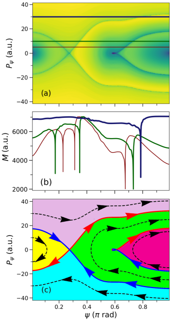
Figure 12: Same as Fig. 11 for the adiabatic potential (9) with $n_{R}=3$. Here, the existence of additional manifolds, associated with the saddle point of the secondary barrier that appears out of the blue in a saddle-node bifurcation, further partitions the phase space in two additional regions.

The width of the new stability region shown in Fig. 12 increases with the integer $n_{R}$. This fact can be seen in Fig. 13, where a similar plot for $n_{R}=6$ is shown. The phase-space structure is essentially the same, but with a larger stable region. Apart from the POs similar to those already presented in Figs. 11(c) and 12(c), we also show in Fig. 13(c) a PO in the stable region, which has the topological shape of a circle. It represents a very particular situation where the Li atom describes a rotation around the C-N at the local minimum ($0.53\pi$ rad) that appears through a dynamical process. The evolution of the phase space for $n_{R}=4,5,7,8$ and 9 can be found in Figs. B.4-B.8 of the Appendix B, respectively. As already mentioned, the area of the stable region increases with the integer $n_{R}$. This fact agrees with the previous discussion on Fig. 10, where it was shown that the height of the local barrier and the distance between the local minimum and the maximum that determines the basin size increase with $n_{R}$.

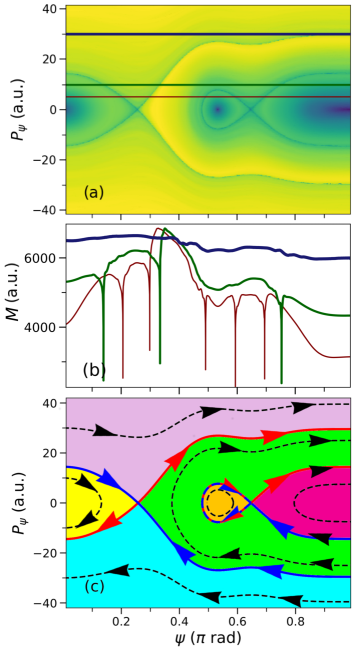
Figure 13: Same as Fig. 12 but for $n_{R}=6$.

V Summary and outlook

In this paper, we have applied the Lagrangian descriptors to identify the invariant manifolds that act as separatrices for the Li-CN$\rightleftharpoons$Li-NC isomerizing reaction, which is a realistic molecular system. We have shown how this tool adequately identifies the previous manifolds as singularities when computed for sufficiently long integration times. Likewise, we have demonstrated that, in general, the adequate computation time must be large enough compared to the inverse of the characteristic stability exponent of the PO of interest. Nonetheless, the previous criterion fails for the case of bifurcating POs, where the characteristic exponents cancel and then their inverses diverge. Moreover, two simplified models have been discussed for a simplified description of the results obtained with the original ab initio PES.

First, we have analyzed the performance of an alternative PES formed by Morse oscillators and also having 2 dof. This equivalent model is also able to reproduce the same structures that appear in one of the saddle-node bifurcations of the system, even when a constant moment of inertia for the angular coordinate is considered.

As an additional simplification, we considered a 1-dof model. To start with, we consider the potential energy in this reduced dimensional model equal to that along the minimum energy path. Such a model is able to reproduce the manifolds that emerge from the top of the energetic barrier of the system, but not those that show up in another saddle-node bifurcation.

As the POs of interest are those with a much faster radial motion than angular motion, an adiabatic approach can be applied to the 2-dof Morse potential, rendering a new energy surface for each quantized level. This 1-dof model is still able to successfully reproduce the main characteristics of the invariant manifolds that emerge from the top of the energetic barrier, as well as those responsible for the appearance of the dynamical barrier for energies $E\geq E_{\rm SN_{1}}=3440.6$ cm^-1. The shape of these last manifolds is strongly influenced by the number of excitations in the stretching motion associated with the radial coordinate, $n_{R}$. Still, the Lagrangian descriptors are also equally able to reproduce them. In this case, the identification of the singularities in the plots of the Lagrangian descriptors has enabled us to unveil the homoclinic intersection that is responsible for the stable island that is observed in the system with 2 dof. Furthermore, we have observed an imprint of the invariant manifolds at smaller energies $E<E_{\rm SN_{1}}$, which are responsible for the appearance of a local minimum in the Lagrangian descriptors plots. Similar results have been also previously reported in Ref. 56, where the effect of the barrier height of a (unbounded) cubic potential is studied. Note, nonetheless, that in our molecular system the height of the energetic barrier cannot be arbitrarily tuned as its value strongly depends on the vibrational energy and, as a consequence, is set by the adiabatic separation of the different degrees of freedom.

To conclude, let us remark that the reduced dimensional models with 1 dof are not able to reproduce all the homoclinic and heteroclinic connections that the system has in its full dimensionality. This limitation is precisely responsible for the easy identification of the manifolds of interest.

Appendix A Phase space for the two-dimensional system

In this appendix A, we discuss the Lagrangian descriptors (LDs) that are shown in Fig. 3 in an extended region of the characteristic Poincaré surface of section for the Li-CN$\rightleftharpoons$CN-Li isomerizing reaction. For this purpose, we show in Fig. A.1 the LDs in the whole Poincaré surface of section accessible at the corresponding energy. As can be seen, the phase space shown in Fig. A.1(a), which is associated with the bifurcating energy $E_{\rm bif}=3440.6$ cm^-1, is divided into two disconnected regions. Consequently, no isomerization can take place, as the Li atom does not have enough energy to overcome the energetic barrier. Notice also the different shape of the LDs in the neighborhood of the parabolic point (purple circle), where the saddle-node bifurcation (SNB) discussed in detail in the main text takes place. When the SNB happens, a stability island appears which opposes isomerization.

Contrarily, when the energy is larger than that of the main energetic barrier, the phase space is formed by a single region, which paves the way for isomerization; this is the case for $E=4000$ cm^-1, as shown in Fig. A.1(b). Notice that the structures that were shown in Fig. 3 of the main text, which emerge due to the SNB, cover quite densely the phase space of the system, creating dozens of homoclinic and heteroclinic connections while folding.

Let us remark on the presence of two important sets that are visible in Fig. A.1(b). On the one hand, the structures emanating from the SNB can be clearly identified, namely the stable island (where the elliptic point shown as a blue triangle is embedded) and the invariant manifolds that surround it (which emerge from the hyperbolic point shown as a red square) can be clearly identified. Consequently, the influence of this structure on the system dynamics cannot be neglected. On the other hand, The invariant manifolds associated with the saddle point that lies at the top of the potential energy barrier (brown diamond), whose evolution is described in more detail in the main text, can be also clearly identified. Therefore, the model proposed with only 1 dof is still capable of reproducing the geometry that surrounds the two barriers that oppose the system reactivity: the barrier top and the SNB.

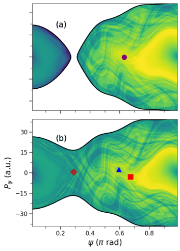
Figure A.​​ 1: Lagrangian descriptors given by Eq. (7) with $p=0.4$ and $\tau=2\times 10^{4}$ a.u. for (a) $E=E_{\rm bif}=3440.6$ cm^-1and for (b) $E=4000$ cm^-1. The purple circle, blue triangle, and red square show the position of the parabolic, elliptic and hyperbolic points associated with the three periodic orbits related to the saddle-node bifurcation under study. The brown diamond shows the position of the unstable periodic orbit that is localized at the energetic barrier top and defines a recrossing-free dividing surface [57, 23].

Appendix B Phase space for the one-dimensional system described with the effective potential

In this appendix B, we report on the phase space geometry associated with the 1-dof model for the LiCN molecule with the adiabatic potential given by Eq. (2) for those vibrational numbers $n_{R}$ that have been omitted in the main text, namely, $n_{R}=0,1,2,4,5,7,8$, and 9. First, we present in Sec. B.1 the phase-space structure for the single-barrier system, which shows up when $n_{R}=0,1,$ and 2. Second, Sec. B.2 is devoted to multiwell situations, a situation that takes place when $n_{R}\geq\leavevmode\nobreak\ 3$.

B.1 Adiabatic potential with a single barrier

Figures B.1(a)-B.3(a) show the value of the LDs for $n_{R}=0,1,$ and 2. As can be seen, the structure is very similar to that already discussed in the Fig. 11. As in that case, the invariant manifolds show up as singularities in the system. These structures have been shown in red (unstable manifold) and blue (stable manifold) continuous lines separately in the Figs. B.1(b)-B.3(b), along with some characteristic periodic orbits (dashed black lines).

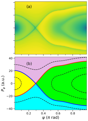
Figure B.​​ 1: Phase space for the LiCN molecular system described by the one-degree-of-freedom model given by Eq. (3) for an effective adiabatic potential with $n_{R}=0$. (a) Lagrangian descriptors computed for $p=0.4$ and $\tau=2\times 10^{4}$ a.u.. (b) The stable (unstable) invariant manifolds that emanate from the saddle point ($\psi\simeq 0.29\pi$ rad), which are shown in blue (red), partition the phase space in the four colored regions.

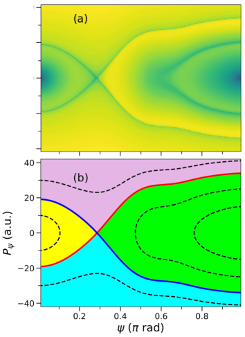
Figure B.​​ 2: Same as Fig. B.1 but for $n_{R}=1$.

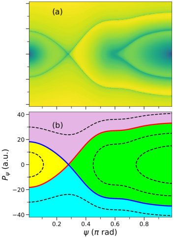
Figure B.​​ 3: Same as Fig. B.1 but for $n_{R}=2$.

B.2 Adiabatic potential with more than one energetic barrier

Figures B.4(a) and B.5(a) show the LDs for $n_{R}=4$ and 5, respectively. Contrary to the previous plots (cf. Figs. B.1-B.3), now two families of invariant manifolds are observed. As already discussed in the main text, the family of invariant manifolds embedded in the green region is associated with the saddle point that emerges due to the SNB, which introduces a secondary energetic barrier. Notice that the area surrounded by the homoclinic connection increases with $n_{R}$, as can be inferred by comparison with Figs. 12 and 13, where the results for $n_{R}=3$ and 6 are respectively shown.

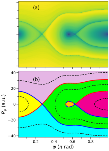
Figure B.​​ 4: Same as Fig. B.1 for $n_{R}=4$. Due to the saddle-node bifurcation, additional manifolds emerge from the saddle point found at $\psi\simeq 0.63\pi$ rad, which further partition the phase space.

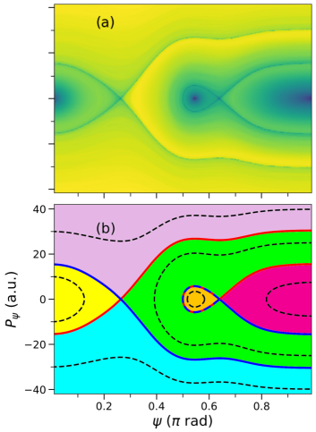
Figure B.​​ 5: Same as Fig. B.4 for $n_{R}=5$.

Figure B.6(a) shows the LDs for $n_{R}=7$. As expected, the stability island has a larger area than in the previous cases discussed. However, in this case an additional structure shows up close to the well $\vartheta=\pi$ rad: the well minimum moves from $\vartheta=\pi$ rad to $\vartheta\simeq 0.90\pi$ rad, with an additional tiny barrier appearing at $\vartheta=\pi$ rad, where a third saddle point can be found. As a consequence, an additional barrier emerges, whose height increases with $n_{R}$. The area occupied by the new stability region also increases with $n_{R}$, as can be inferred from comparison with Figs. B.7 and B.8, where the results for $n_{R}=8$ and 9 are shown. Notice in Fig. B.6(b), where the invariant manifolds of Fig. B.6(a) are shown, that the second stability region is also surrounded by a homoclinic orbit. Contrary to the stability region discussed in connection to the 2-dof system, the one that appears for $n_{R}\geq 7$ does not have an imprint on that system. As a consequence, it is produced solely by the adiabatic approximation, thus demonstrating the limitations of this approach.

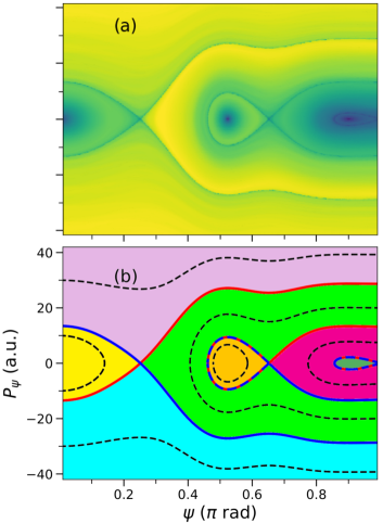
Figure B.​​ 6: Same as Fig. B.4 for $n_{R}=7$. The invariant manifolds associated with the spurious saddle-point that is found at $\psi=\pi$ rad, and were absent for $n_{R}\leq 6$, have been colored as dashed blue and red lines.

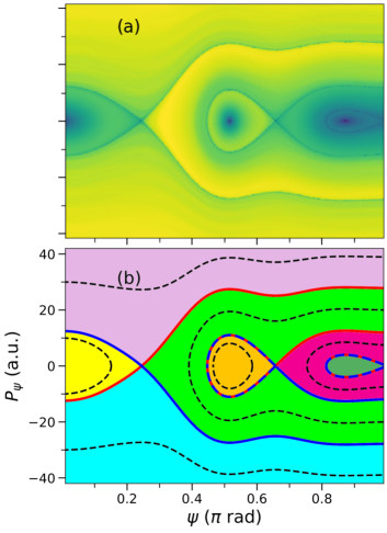
Figure B.​​ 7: Same as Fig. B.6 but for $n_{R}=8$.

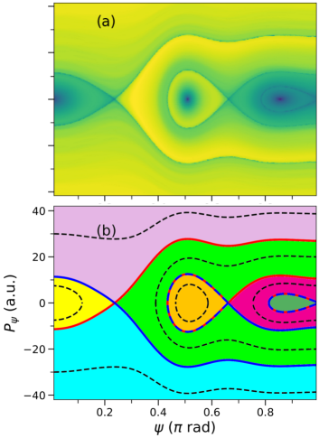
Figure B.​​ 8: Same as Fig. B.6 but for $n_{R}=9$.

References

- Levine [1975] I. N. Levine, Molecular Spectroscopy (Wiley, 1975).
- Karmakar and Keshavamurthy [2020] S. Karmakar and S. Keshavamurthy, Phys. Chem. Chem. Phys. 22, 11139 (2020).
- Worth and Cederbaum [2004] G. A. Worth and L. S. Cederbaum, Ann. Rev. Phys. Chem. 55, 127 (2004).
- Polli et al. [2010] D. Polli, P. Altoè, O. Weingart, K. Spillane, C. Manzoni, D. Brida, G. Tomasello, G. Orlandi, P. Kukura, R. Mathies, M. Garavelli, and G. Cerullo, Nature 467, 440 (2010).
- Jiang and Sibert [2012] R. Jiang and E. L. Sibert, J. Chem. Phys. 136, 224104 (2012).
- Lichtenberg and Lieberman [2010] A. J. Lichtenberg and M. A. Lieberman, Regular and Stochastic Motion, Applied Mathematical Sciences, Vol. 38 (Springer, 2010).
- Fujisaki and Straub [2005] H. Fujisaki and J. E. Straub, Proc. Natl. Acad. Sci. USA 102, 6726 (2005).
- Arnold et al. [2006] I. Arnold, S. M. Gusein-Sade, and A. N. Varchenko, Mathematical aspects of classical and celestial mechanics, (2006).
- Birkhoff [1913] G. D. Birkhoff, Trans. Amer. Math. Soc. 14, 14 (1913).
- Marcus [1992] R. A. Marcus, Science 256, 1523 (1992).
- Marcelin [1915] M. R. Marcelin, Ann. Phys. 9, 120 (1915).
- Wigner [1938] E. Wigner, Trans. Faraday Soc. 34, 29 (1938).
- Truhlar et al. [1996] D. G. Truhlar, B. C. Garrett, and S. J. Klippenstein, J. Phys. Chem. 100, 12771 (1996).
- Jaffé et al. [2000] C. Jaffé, D. Farrelly, and T. Uzer, Phys. Rev. Lett. 84, 610 (2000).
- Jaffé et al. [2002] C. Jaffé, S. D. Ross, M. W. Lo, J. Marsden, D. Farrelly, and T. Uzer, Phys. Rev. Lett. 89, 011101 (2002).
- Uzer et al. [2002] T. Uzer, C. Jaffé, J. Palacián, P. Yanguas, and S. Wiggins, Nonlinearity 15 (4), 957 (2002).
- de Oliveira et al. [2002] H. P. de Oliveira, A. M. Ozorio de Almeida, I. Damião Soares, and E. V. Tonini, Phys. Rev. D 65, 083511 (2002).
- Gorban and Karlin [2005] A. N. Gorban and I. V. Karlin, Invariant manifolds for physical and chemical kinetics, 1st ed., Lecture Notes in Physics 660 (Springer-Verlag Berlin Heidelberg, 2005).
- Miller [1998] W. H. Miller, Faraday Discuss. 110, 1 (1998).
- Althorpe and Hele [2013] S. C. Althorpe and T. J. H. Hele, J. Chem. Phys. 139, 084115 (2013).
- Jang and Voth [2016] S. Jang and G. A. Voth, J. Chem. Phys. 144, 084110 (2016).
- Hele and Althorpe [2016] T. J. H. Hele and S. C. Althorpe, J. Chem. Phys. 144, 174107 (2016).
- Pechukas and Pollak [1977] P. Pechukas and E. Pollak, J. Chem. Phys. 67, 5976 (1977).
- Bartsch et al. [2005] T. Bartsch, R. Hernandez, and T. Uzer, Phys. Rev. Lett. 95, 058301 (2005).
- Kawai et al. [2007] S. Kawai, A. D. Bandrauk, C. Jaffé, T. Bartsch, J. Palacián, and T. Uzer, J. Chem. Phys. 126, 164306 (2007).
- Bartsch et al. [2012] T. Bartsch, F. Revuelta, R. M. Benito, and F. Borondo, J. Chem. Phys. 136, 224510 (2012).
- Revuelta et al. [2012] F. Revuelta, T. Bartsch, R. M. Benito, and F. Borondo, J. Chem. Phys. 136, 091102 (2012).
- Craven and Hernandez [2015] G. T. Craven and R. Hernandez, Phys. Rev. Lett. 115, 148301 (2015).
- Bartsch et al. [2019] T. Bartsch, F. Revuelta, R. M. Benito, and F. Borondo, Phys. Rev. E 99, 052211 (2019).
- Davis and Heller [1981] M. J. Davis and E. J. Heller, J. Chem. Phys. 75, 246 (1981).
- Borondo et al. [1995] F. Borondo, A. Zembekov, and R. Benito, Chem. Phys. Lett. 246, 421 (1995).
- Borondo et al. [1996] F. Borondo, A. A. Zembekov, and R. M. Benito, J. Chem. Phys. 105, 5068 (1996).
- Zembekov et al. [1997] A. A. Zembekov, F. Borondo, and R. M. Benito, J. Chem. Phys. 107, 7934 (1997).
- Müller et al. [2012] P. L. G. Müller, R. Hernandez, R. M. Benito, and F. Borondo, J. Chem. Phys. 137, 204301 (2012).
- Jiménez-Madrid and Mancho [2009] J. A. Jiménez-Madrid and A. M. Mancho, Chaos 19, 013111 (2009).
- Lopesino et al. [2015] C. Lopesino, F. Balibrea-Iniesta, S. Wiggins, and A. M. Mancho, Comm. Nonlin. Sci. Num. Sim. 27, 40 (2015).
- Essers et al. [1982] R. Essers, J. Tennyson, and P. E. S. Wormer, Chem. Phys. Lett. 89, 223 (1982).
- Benito et al. [1989] R. Benito, F. Borondo, J.-H. Kim, B. Sumpter, and G. Ezra, Chemical Physics Letters 161, 60 (1989).
- Revuelta et al. [2017] F. Revuelta, E. Vergini, R. M. Benito, and F. Borondo, J. Chem. Phys. 146, 014107 (2017).
- Revuelta et al. [2019] F. Revuelta, R. M. Benito, and F. Borondo, Phys. Rev. E 99, 032221 (2019).
- Prosmiti et al. [1996] R. Prosmiti, S. C. Farantos, R. Guantes, F. Borondo, and R. M. Benito, J. Chem. Phys. 104, 2921 (1996).
- Arranz et al. [2000] F. Arranz, F. Borondo, and R. Benito, Chemical Physics Letters 317, 451 (2000).
- Iñarrea et al. [2011] M. Iñarrea, J. F. Palacián, A. I. Pascual, and J. P. Salas, J. Chem. Phys. 135, 014110 (2011).
- Allahem and Bartsch [2012] A. Allahem and T. Bartsch, J. Chem. Phys. 137, 214310 (2012).
- Keating and Prado [2001] J. P. Keating and S. D. Prado, Proc. Royal Soc. London. Series A: Math., Phys. and Eng. Sci. 457, 1855 (2001).
- Revuelta et al. [2016a] F. Revuelta, E. Vergini, R. M. Benito, and F. Borondo, J. Phys. Chem. A 120, 4928 (2016a).
- Joyeux et al. [2002] M. Joyeux, S. C. Farantos, and R. Schinke, J. Phys. Chem. A 106, 5407 (2002).
- Schomerus and Sieber [1997] H. Schomerus and M. Sieber, J. Phys. A 30, 4537 (1997).
- García-Müller et al. [2008] P. L. García-Müller, F. Borondo, R. Hernandez, and R. M. Benito, Phys. Rev. Lett. 101, 178302 (2008).
- Revuelta et al. [2016b] F. Revuelta, T. Bartsch, P. L. Garcia-Muller, R. Hernandez, R. M. Benito, and F. Borondo, Phys. Rev. E 93, 062304 (2016b).
- Mancho et al. [2013] A. M. Mancho, S. Wiggins, J. Curbelo, and C. Mendoza, Comm. Nonlin. Sci. Num. Sim. 18, 3530 (2013).
- Montes et al. [2021] J. Montes, F. Revuelta, and F. Borondo, Comm. Nonlin. Sci. Num. Sim. 102, 105860 (2021).
- Carlo and Borondo [2020] G. G. Carlo and F. Borondo, Phys. Rev. E 101, 022208 (2020).
- Junginger et al. [2016] A. Junginger, P. L. Garcia-Muller, F. Borondo, R. M. Benito, and R. Hernandez, J. Chem. Phys. 144, 024104 (2016).
- Light and Bačić [1987] J. C. Light and Z. Bačić, J. Chem. Phys. 87, 4008 (1987).
- García-Garrido et al. [2020] V. J. García-Garrido, S. Naik, and S. Wiggins, Int. J. Bif. and Chaos 30, 2030008 (2020).
- Pechukas and McLafferty [1973] P. Pechukas and F. J. McLafferty, J. Chem. Phys. 58, 1622 (1973).