Fully Three-dimensional Radial Visualization

Abstract

We develop methodology for three-dimensional (3D) radial visualization (RadViz) of multidimensional datasets. The classical two-dimensional (2D) RadViz visualizes multivariate data in the 2D plane by mapping every observation to a point inside the unit circle. Our tool, RadViz3D, distributes anchor points uniformly on the 3D unit sphere. We show that this uniform distribution provides the best visualization with minimal artificial visual correlation for data with uncorrelated variables. However, anchor points can be placed exactly equi-distant from each other only for the five Platonic solids, so we provide equi-distant anchor points for these five settings, and approximately equi-distant anchor points via a Fibonacci grid for the other cases. Our methodology, implemented in the R package radviz3d, makes fully 3D RadViz possible and is shown to improve the ability of this nonlinear technique in more faithfully displaying simulated data as well as the crabs, olive oils and wine datasets. Additionally, because radial visualization is naturally suited for compositional data, we use RadViz3D to illustrate (i) the chemical composition of Longquan celadon ceramics and their Jingdezhen imitation over centuries, and (ii) US regional SARS-Cov-2 variants’ prevalence in the Covid-19 pandemic during the summer 2021 surge of the Delta variant.

I Introduction

Graphical display of multivariate data is important to obtain insight into their properties and similarity or distinctiveness of different groups [1]. The goal of effective visualization is to map multi-dimensional observations to a lower-dimensional space, with the reduced display conveying information on the characteristics as faithfully as possible.

Continuous multivariate data are displayed in many ways [2, 3] (e.g. starplots  [4], Chernoff faces [5], parallel coordinate plots [6, 7], surveyplots [8], Andrews’ curves [9, 10], biplots [11], star coordinate plots [12],the grand tour [13, 14], Uniform Manifold Approximation and Projections (UMAP) [15]), but our focus in this short technical note is on improving the nonlinear display called radial visualization or RadViz [16, 17, 18, 19] that projects data onto a circle using Hooke’s law. Here, $p$-dimensional observations are projected onto the 2D plane using $p$ anchor points arranged to be on the perimeter of a circle. This representation places each observation at the center of the circle that is then pulled by springs in the directions of the $p$ anchor points while being balanced by forces relative to the coordinate values. Observations with similar relative values across all attributes are placed close to the center while the others are closer to anchor points corresponding to the coordinates with higher relative values. However, there is loss of information [20] in RadViz which maps a $p$-dimensional point to 2D. This loss worsens with increasing $p$, but may potentially be alleviated by extending it to 3D. The Viz3D approach [20] extends 2D RadViz (henceforth, RadViz2D) by simply adding to the 2D projection a third dimension that, for each observation, is simply the average of all its attributes. The extension robs Viz3D of its interpretability in terms of the attributes. Its improvement over RadViz2D is also by design limited, so here we investigate the possibility of developing a truly 3D extension of RadViz.

One challenge of extending RadViz from two to three dimensions is that a 3D sphere can be exactly divided into $p$ regions of equal volumes only for the Platonic solids. However, Section II shows that placing equi-spaced anchor points is necessary to reduce artificially induced correlation between variables. So, for other $p$, Section II uses a Fibonacci grid method to develop an approximate solution. We call our method RadViz3D and illustrate in Section III its ability to more accurately display structure in simulated and some common real datasets, than RadViz2D or Viz3D. Further, because radial visualization is, by construction, naturally suited for compositional data, we use RadViz3D on two such datasets. In the first case, we illustrate the composition, over history, of celadon ceramics from Longquan kilns and that of their Jingdezhen kiln-manufactured imitations. Our second example uses RadViz3D to illustrate the changing face of the Covid-19 pandemic in the ten Health and Human Services (HHS) regions of the United States (US) over the course of the summer of 2021, in terms of the proportion of the variants ofthe Severe Acute Respiratory Syndrome Coronavirus 2 (SARS-Cov-2). The main paper concludes with some discussion. We also have an online supplemental HTML resource (also at https://radviz3d.github.io) that allows the reader to more fully experience the benefits of RadViz3D (and Viz3D) on our examples.

II Methodology

II-A Generalized radial visualization

We naturally extend the classic RadViz2D by defining generalized radial visualization (GRadViz) as a map of $\bm{X}=(X_{1},X_{2},\ldots,X_{p})^{\top}\in\mathbb{R}^{p}$ to a point in $\mathbb{S}^{q}=\{\bm{x}\in\mathcal{R}^{q+1}:\|\bm{x}\|=1\}$ using

$$\bm{\Psi}(\bm{X};\bm{U})=\frac{\bm{U}\bm{X}}{\bm{1}_{p}^{\top}\bm{X}},$$ (1)

where $\bm{1}_{p}=(1,1,\ldots,1)^{\top}$, and $\bm{U}=[\bm{u}_{1}\vdots\bm{u}_{2}\vdots\ldots\vdots\bm{u}_{p}]$ is a projection matrix with $j$th column and anchor point $\bm{u}_{j}\in\mathbb{S}^{q}$, for $j=1,2,\ldots,p$. For $q=1$, GRadViz reduces to RadViz2D.

Remark 1.

As helpfully suggested by a reviewer, the use of $\bm{X}/\bm{1}^{\top}\bm{X}$ in (1) means that it is ideally set up for compositional data. We illustrate performance with such data in Sections III-C1 and III-C2.

As in RadViz2D, our generalization $\bm{\Psi}(\cdot;\cdot)$ also has a physical interpretation. Suppose that we have $p$ springs connected to the anchor points $\bm{u}_{1},\bm{u}_{2},\ldots,\bm{u}_{p}\in\mathbb{S}^{q}$ and that these $p$ springs have spring constants $X_{1},X_{2},\ldots,X_{p}$. Let $\bm{Y}\in\mathcal{R}^{q+1}$ be the equilibrium point of the system. Then we have $\sum_{j=1}^{p}X_{j}(\bm{Y}-\bm{u}_{j})=0,$ with our generalization $\bm{Y}=\bm{\Psi}(\bm{X};\bm{U})$ as its solution.

GRadViz is actually a special case of normalized radial visualization (NRV) [21] that allows the anchor points to lie outside the hypersphere and is point-ordering-, line-ordering-, and convexity-invariant. These desirable properties for visualization are also inherited by $\bm{\Psi}(\cdot;\cdot)$. However, GRadViz is scale-invariant, that is, $\bm{\Psi}(k\bm{X};\bm{U})\!=\!\bm{\Psi}(\bm{X};\bm{U})$ for any $k\neq 0$. In other words, any line passing through the origin is projected to a single point in the radial visualization. So the visualization is invariant under scaling, and only the relative values of the coordinates matter. This means that the coordinates of the dataset have to be comparable, so we use the minmax transformation on the $j$th feature ($j=1,2,\ldots,p$) of the $i$th observation that is given by

$$m_{j}(X_{ij})=\frac{X_{ij}-\min_{1\leq i\leq n}X_{ij}}{\max_{1\leq i\leq n}X_{ij}-\min_{1\leq i\leq n}X_{ij}}.$$ (2)

The minmax transformation places every observation in $[0,1]^{p}$, ensuring that the data, after also applying $\bm{\Psi}(\cdot;\cdot)$, are all inside the unit ball $\mathbb{B}^{q+1}=\{\bm{x}\in\mathcal{R}^{q+1}:\|x\|\leq 1\}$. Outliers, if any, are placed close to the boundary of the ball. Other standardization teciniques like centering and scaling do not enjoy these properties, so we use the minmax transformation as the default standardization for this article.

The placement of the anchor points is another issue to be addressed in GRadViz, with different points yielding very different visualizations. Now suppose that $\bm{X}$ has $p$ uncorrelated coordinates. For any $\bm{X}_{i},\bm{X}_{j}\in{\mathcal{R}}^{p}$, let $\bm{Y}_{l}=\bm{\Psi}(\bm{X}_{l};\bm{U}),l\in\{i,j\}$ be the GRadViz-transformed data. The squared Euclidean distance between $\bm{Y}_{i}$ and $\bm{Y}_{j}$ is

$$\|\bm{Y}_{i}-\bm{Y}_{j}\|^{2}=\left(\frac{\bm{X}_{i}}{\bm{1}_{p}^{\top}\bm{X}_{i}}-\frac{\bm{X}_{j}}{\bm{1}_{p}^{\top}\bm{X}_{j}}\right)^{\top}\bm{U}^{\top}\bm{U}\left(\frac{\bm{X}_{i}}{\bm{1}_{p}^{\top}\bm{X}_{i}}-\frac{\bm{X}_{j}}{\bm{1}_{p}^{\top}\bm{X}_{j}}\right),$$

a quadratic form with positive definite matrix $\bm{U}^{\top}\bm{U}$ that has the $l$th diagonal element $\bm{u}_{l}^{\top}\bm{u}_{l}=1$ and $(k,l)$th entry $\bm{u}_{k}^{\top}\bm{u}_{l}=\cos\langle\bm{u}_{k},\bm{u}_{l}\rangle$. For $\bm{X}_{l}=a_{l}\bm{e}_{l}$, with $\bm{e}_{l}$ as the $l$th standard unit vector ($l\in\{i,j\}$),

$$\|\bm{Y}_{i}-\bm{Y}_{j}\|^{2}=2-2\cos(\bm{u}_{i},\bm{u}_{j}).$$ (3)

The $i$th and $j$th coordinates of $\bm{X}_{i}$ and $\bm{X}_{j}$ in this example are as discordant as possible from each other (which is very likely to happen if $i$th and $j$th coordinates are negatively correlated or uncorrelated), playing an important role in identifying distinctive data points, and should be placed as far apart as possible (in opposite directions) in the radial visualization. However (3) shows that the squared Euclidean distance between $\bm{Y}_{i}$ and $\bm{Y}_{j}$ approaches 0 as the angle between $\bm{u}_{i}$ and $\bm{u}_{j}$ approaches 0. Therefore, the radial visualization will display such points to be more similar and fails to acknowledge the differences in the $i$th and the $j$th coordinates if the angle between $\bm{u}_{i}$ and $\bm{u}_{j}$ is less then $\pi/2$, which can create artificial positive visual correlation between the $i$th and $j$th coordinates (positive visual correlation here means that visualization will be like the case when the $i$th and the $j$th coordinates are positively correlated). Since not all pairs of coordinates will be negatively correlated, when two coordinates are positively correlated, they are less important in differentiating distinctive data points and therefore positively correlated coordinates should be placed close together so that there is more room to place negatively correlated coordinates apart. When all coordinates are uncorrelated, they are equally important in differentiating distinctive data points. To reduce such effects, we need to distribute the anchor points as far away from each other as possible. Therefore, our GRadViz formulation recommends evenly-distributed anchor points on $\mathbb{S}^{q}$. RadViz3D has an inherent advantage over RadViz2D because it can more readily facilitate larger angles between anchor points as the smallest angle between any two of $p$ (fixed) evenly-distributed anchor points in RadViz3D is always larger than that in RadViz2D. (Indeed, higher-dimensional displays beyond 3D would be even more beneficial were it possible to obtain such displays.) For example, with $p=4$, we can place anchor points in 3D so that the angle between any two of them is the same, but this is not possible in 2D. At the same time, RadViz2D can not place multiple positively correlated coordinates next to each other, as desirable for accurate visualization [22]. The placement of anchor points therefore has more pronounced importance in RadViz2D [23, 24] than RadViz3D.

Remark 2.

Our discussion on GRadViz provides the rationale behind radial visualization with equi-spaced anchor points. It also shows that investigating spacings between anchor points, as done [23, 25, 26] for RadViz2D, is unnecessary and perhaps even misleading because of its potential to induce artificial visual correlation between coordinates. However, as pointed out by a reviewer, investigating layouts and arrangements of the axes is still important for cases with $p>3$ in RadViz2D, and $p>4$ for RadViz3D.

II-B Three-dimensional radial visualization

Following the setup and discussion in Section II-A, let $\bm{\Psi}:\mathbb{R}^{p}\mapsto\mathbb{B}^{3}=\{\bm{x}\in{{\mathbb{R}}^{3}}:\|\bm{x}\|\leq 1\}$ map $\bm{X}\in\mathbb{R}^{p}$ to $\bm{\Psi}(\bm{X};\bm{U})=\bm{U}\bm{X}/\bm{1}_{p}^{\top}\bm{X}$ with $\bm{U}$ as before and with $j$th column (anchor point) $\bm{u}_{j}$ that, we have contended, should be as evenly-spaced in $\mathbb{S}^{2}$ as possible. We find the set $\wp$ of equi-spaced anchor points $\bm{u}_{1},\bm{u}_{2},\ldots,\bm{u}_{p}$ from Result 3.

Result 3.

Anchor Points Set. Denote the golden ratio by $\varphi=(1+\sqrt{5})/2$. For $p\in\{4,6,8,12,20\}$, the elements in $\wp$ have the coordinates listed in Table I.

TABLE I: Anchor points set for $p\!\in\!\{4,6,8,12,20\}$. Here $\varphi\!=\!(1\!+\!\sqrt{5})/2$.

$p$	Platonic Solid	$\wp$
4	Tetrahedron	$\{(1,1,1)/\sqrt{3},(1,-1,-1)/\sqrt{3},(-1,1,-1)/\sqrt{3},(-1,-1,1)/\sqrt{3}\}$
6	Octahedron	$\{(\pm 1,0,0),(0,\pm 1,0),(0,0,\pm 1)\}$
8	Cube	$\{\pm 1,\pm 1,\pm 1\}$
12	Dodecahedron	$\{(0,\pm 1,\pm\varphi),(\pm 1,\pm\varphi,0)(\pm\varphi,0,\pm 1)\}/\sqrt{1+\varphi^{2}}$
20	Icosahedron	$\{(\pm 1,\pm 1,\pm 1)/\sqrt{3},(0,\pm\varphi^{-1},\pm\varphi)/\sqrt{3},(\pm\varphi^{-1},\pm\varphi,1)/\sqrt{3},(\pm\psi,0,\pm\varphi^{-1})/\sqrt{3}\}$

For other integers $p\geq 5$, only an approximate solution is possible: here the elements of $\wp$ are $\bm{u}_{j}^{\top}=(u_{j1},u_{j2},u_{j3}),j=1,2,\ldots,p$ with $u_{j1}=\cos(2\pi j\varphi^{-1})(1-u_{j3}^{2})^{-\frac{1}{2}},u_{j2}=\sin(2\pi j\varphi^{-1})(1-u_{j3}^{2})^{-\frac{1}{2}},u_{j3}=(2j-1)/p-1.$

Proof.

For $p\in\{4,6,8,12,20\}$, the coordinates are exactly equi-spaced with anchor points corresponding to the vertices of the Platonic solids. For other values of $p\geq 5$, we derive an approximate solution by implementing a Fibonacci grid method [27] that produces the latitude $\phi_{j}$ and longitude $\theta_{j}$ of the $j$th anchor point on $\mathbb{S}^{3}$ as $\phi_{j}=\arcsin a_{j},\theta_{j}=2\pi j\varphi^{-1}$ with $a_{1},a_{2},\ldots,a_{p}$ an arithmetic progression chosen to have common difference $\displaystyle{{2}/{p}}$. We take $a_{1}=\displaystyle{{1}/{p}-1}$, so $a_{j}={2}(j-1)/p+a_{1}=({2j-1})/{p}-1$. The Cartesian coordinates of the $j$th anchor point $\bm{u}_{j}\in\wp$ follow by transforming between coordinate systems. ∎

Remark 4.

The geometric solutions of $\wp$ for $p\in\{4,6,8,12,20\}$ are closely related to the Thomson problem in traditional molecular quantum chemistry [28]. Also, for $p\geq 5$, $p\not\in\{4,6,8,12,20\}$, the approximate solution distributes anchor points along a generative spiral on $\mathbb{S}^{2}$, with consecutive points as separated from each other as possible, satisfying the “well-separation” property [29].

Result 3 provides the wherewithal for RadViz3D for $p\geq 4$ by projecting each observation $\bm{X}_{i}\in\mathbb{R}^{p},i=1,2,\ldots,n$ to $\bm{\Psi}(\bm{X}_{i};\bm{U}=[\bm{u}_{1}\vdots\bm{u}_{2}\vdots\ldots\vdots\bm{u}_{p}])$. RadViz3D displays of multidimensional data can then be obtained via 3D graphics to facilitate the discovery of patterns and structure.

III Illustrative Examples

We illustrate RadViz3D on some moderately-dimensioned simulated and standard classification datasets and show that it can reveal distinctiveness of class and other structure better than RadViz2D or Viz3D. Because RadViz3D and Viz3D are 3D displays, we only show some of their static views in this paper, referring the reader to the HTML resource for their fuller appreciation. Further, we use the overlap heatmap of $\bm{\Omega}$ to display the numerical distinctiveness of each class relative to the others. We define $\bm{\Omega}$ in the following way. Let $\omega_{j\mid i}$ be the probability of misclassifying an observation from the $i$th group into the $j$th group. Then $\bm{\Omega}$ is the symmetrized matrix with $(i,j)$th element consisting of the pairwise overlap [30] $\omega_{ij}=\omega_{j\mid i}+\omega_{i\mid j}$. The overlap heatmap displays $\omega_{ij}$ for $i>j$.

III-A Simulated datasets

We simulated 5D datasets of $n=500$ observations from five groups of known group separation and clustering complexity. The MixSim package [31] in R [32] allows for the simulation of class data according to a pre-specified generalized overlap ($\ddot{\omega}$) measure [33] that indexes clustering complexity, with a

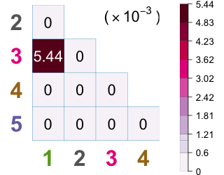
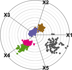
() $\ddot{\omega}=0.001$

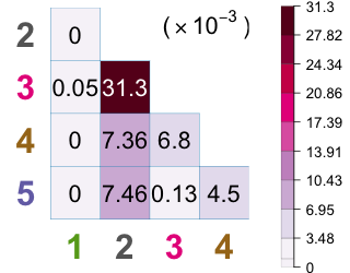
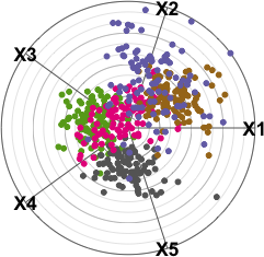
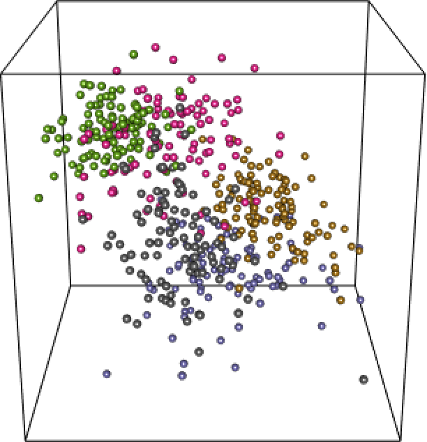
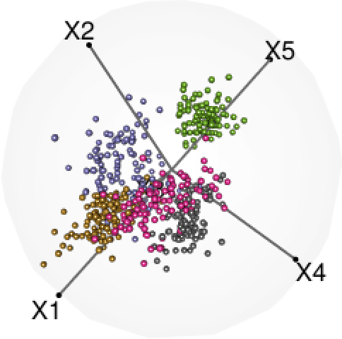
() $\ddot{\omega}=0.01$

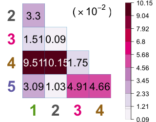
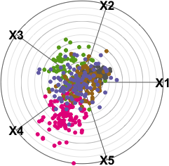
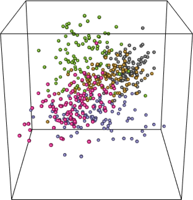
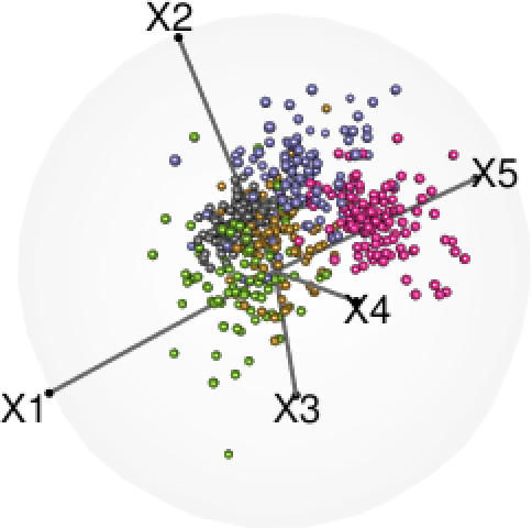
() $\ddot{\omega}=0.05$

Figure 1: Overlap heatmaps of $\bm{\Omega}$ and RadViz2D, Viz3D and RadViz3D displays of simulated 5D datasets of varying clustering complexity ($\ddot{\omega}$). Colors of class labels are the same for each setting.

small value ($\ddot{\omega}\!\!=\!\!10^{-3}$) implying good separation between groups and larger values ($\ddot{\omega}=0.01,0.05$) indicating increasingly poorer separation and increased overlap. Fig. 1 displays the results and shows that the MixSim-generated pairwise overlaps between the 5 groups are essentially preserved in the RadViz3D display. For $\ddot{\omega}\!\!=\!\!10^{-3}$ (Fig. 1a), the relatively higher overlap between Groups 1 and 3 is captured across all three displays, but unlike RadViz3D, both RadViz2D and Viz3D place both Groups 4 and 5 fairly close together, belying their good separation ($\omega_{45}\approx 0$). The more appropriate use of the third dimension by RadViz3D than by Viz3D provides greater benefit at higher $\ddot{\omega}$. For instance, Viz3D and RadViz2D show little qualitative difference in the distinctiveness of the groups between Figs. 1b and 1c, but RadViz3D shows that while the five classes are less separated in Fig. 1b than in Fig. 1a, the groups are still fairly distinguishable here relative to Fig. 1c. Therefore, the RadViz3D display provides a more accurate and meaningful representation of the known class structure of these datasets.

III-B Some common real-data examples

We now visualize three multivariate datasets often used in the statistical graphics literature.

III-B1 Crabs

This dataset [34] has measurements on morphological characteristics (FL or frontal lip width, RW or rear width, CL or carapace midline length, CW or carapace maximum width, BD or body depth) of 50 crabs each with blue or orange shells and of each gender. Fig. 2 shows the three displays along with the overlap heatmap of $\bm{\Omega}$.

Male-Blue Female-Blue Male-Orange Female-Orange

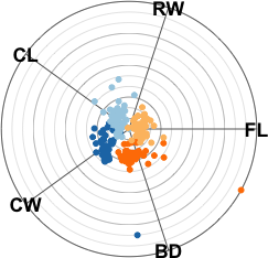
(a) RadViz2D

(b) Viz3D

(c) RadViz3D

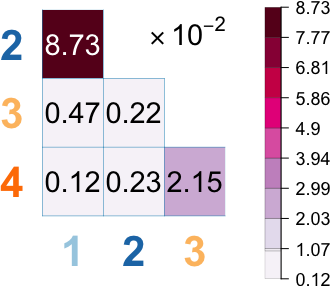
(d) Overlap heatmap

Figure 2: RadViz2D, Viz3D, RadViz3D displays and the overlap heatmap of the Crabs dataset.

We see less distinction between the males and females as per $\bm{\Omega}$, but that is not quite captured in the RadViz2D displays (and definitely not so in Viz3D). However, the RadViz3d display indicates that CL may be redundant in the display, as also reported in [35]. Removing this variable results in a clearer display (Fig. 3) where the RadViz3D display shows not just the higher overlap between the blue males and females relative to those between the orange males and females, but also that the species are less distinguishable, in terms of these characteristics, in the males than in the females.

Male-Blue Female-Blue Male-Orange Female-Orange

(a) RadViz2D

(b) Viz3D

(c) RadViz3D

(d) Overlap Map

Figure 3: Radial visualization displays and overlap heatmap of the Crabs dataset sans CL.

In this illustration, RadViz3D is seen to alone provide important information on the structure of the data in terms of identifying both the redundancy of CL as well as faithful distinction between the classes.

III-B2 Wine

This dataset [36] is on the chemical composition of 178 wines from three (Barolo, Gringolino and Barbera) cultivars

Cultivar 1 Cultivar 2 Cultivar 3

(a) RadViz2D

(b) Viz3D

(c) RadViz3D

Figure 4: RadViz2D, Viz3D and RadViz3D displays of the Wine dataset.

of grapes grown in the same region of Italy. Fig. 4 provides the three displays of the dataset through the composition of thirteen chemicals: Alcohol (Ahl), Malic acid (Malic), Ash, Alkalinity of ash (Alk), Magnesium (Mg), Total phenols (Pnls), Flavanoids (Flvds), Nonflavanoid phenols (Nonfp), Proanthocyanins (Pthyns), Color intensity, Hue, OD280/OD315 of diluted wines (ODdil) and Proline (Prol). All three displays can not correctly distinguish the first two cultivars from each other but RadViz3D alone separates the third cultivar from the others very well, more accurately reflecting the overlap measures $(\omega_{13}\approx 0,\omega_{23}\approx 9\times 10^{-4})$.

III-B3 Olive oils

This dataset [37, 38] provides the composition of eight fatty (palmitic, palmitoleic, stearic, oleic, linoleic, linolenic, arachidic, eicosenoic) acids in 572 olive oil samples from nine regions in three areas of Italy.

Coast-Sardinia Inland-Sardinia Umbria East-Liguria West-Liguria
North-Apulia South-Apulia Calabria Sicily

(a) RadViz2D

(b) Viz3D

(c) Overlap Map

(d) RadViz3D, Sardinia

(e) RadViz3D, Northern Italy

(f) RadViz3D, Southern Italy

Figure 5: Olive oils dataset: (a) RadViz2D and (b) Viz3d displays, and (c) Overlap map $\bm{\Omega}$. (d-f) RadViz3D displays, each showing the distinctiveness of an area’s olive oils.

Two regions are (Coastal and Inland) Sardinian, while three (Umbria, East and West Liguria) are from northern Italy and four (North and South Apulia, Calabria, Sicily) are from the South. Fig. 5 shows West Liguria is separated in all three visualizations, but only RadViz3D (Fig. 5d) distinguishes coastal and inland Sardinia oils from the others. The northern regions are reasonably distinguished from each other in RadViz3D and well-separated from the other areas (for both 3D methods, though RadViz3D is clearer). The southern regions are difficult to distinguish from each other but more easily distinguished from the north and Sardinia. [39] reported two groups in the southern oils, with North Apulia more distinct than the rest, and our displays (Fig. 5d,e) support this view. Our displays also echo [40]’s findings that olive oils are easier distinguished by area than by region.

III-C Compositional datasets

We visualize two compositional datasets not hitherto analyzed in the statistics literature.

III-C1 Illustrating the history of Chinese celadon ceramics

Song Yuan Ming Qing
Body Glaze
Imitated Longquan Longquan celadon

(a) RadViz2D

(b) Viz3D

(a) RadViz3D

Figure 6: RadViz2D, Viz3D and RadViz3D displays of the celadons dataset.

Longquan celadon [41, 42] is a type of green-glazed Chinese ceramic with a long history of production at its namesake site. It received a major production boost in the Northern Song (960–1127) period, continuing under the Southern Song (1127–1279), Yuan (1271–1368), Ming (1368–1644) and Qing (1644–1912) dynasties. These celadons were much coveted, becoming an important part of China’s export economy for over five hundred years and widely imitated, for instance at Jingdezhen, whose famed blue and white porcelain finally overtook the Longquan celadon. Samples of Longquan celadon manufactured in Dayao from the above periods and their imitations manufactured in Jingdezhen during the Ming period, were analyzed [43] by means of the composition of 17 compounds (Na₂O, MgO, Al₂O₃, SiO₂, K₂O, CaO, TiO₂, Fe₂O₃, MnO, CuO, ZnO, PbO₂, Rb₂O, SrO, Y₂O₃, ZrO₂ and P₂O₅). In all, chemical compositions of these compounds on the body and glaze of 44 celadon samples are available, and also included in the celadons dataset of our radviz3D package. Fig. 6 displays the dataset in terms of the compositions of the 17 compounds. The RadViz2D and Viz3D displays are largely uninformative, but RadViz3D illustrates well the history of Longquan celadon and its imitation. The chemical composition of celadon glaze and body are distinct from each other. RadViz3D also clearly separates Longquan body from its imitation. This accurately reflects the view that soils used in the manufacture of celadon were acquired locally by the Jingdezhen craftsmen for reasons of cost due to high demand of the celadon body raw materials. Further, archaelogical excavations [44] indicate that Jingdezhen soils have lower Fe₂O₃ and TiO₂ content and higher silica (CaO) than soils at the Dayao sites. As in [43], our display also indicates distinctiveness of genuine Longquan glaze from its imitation, but there is improvement over time, so much so that some later Longquan samples (Qing period) are close in composition to the Jingdezhen samples. Genuine Longquan chemical composition itself evolved over the four dynasties, as indicated in the figure. In summary, our RadViz3D display of this compositional dataset provides clearer and more interpretable displays than RadViz2D or Viz3D.

III-C2 Tracking SARS-Cov-2 variant proportions in the US

The closing months of 2019 saw the emergence of the SARS-Cov-2 virus in Wuhan, China followed by its rapid spread around the world to become the most disruptive global pandemic in over a century. Several vaccines were developed in record time, and multi-phased vaccinations started in several countries, including in the US in early 2021. However, evolution of the virus brought new variants, some deadlier and more transmissible. After the Delta variant arrived in the US, it virtually engulfed healthcare systems over the summer of 2021. Here, we illustrate the changing proportions of the SARS-Cov-2 variants in the ten US HHS regions during the rapid transition to Delta.

Our dataset is from the most recent (per October 5, 2021) weekly average proportions of 12 sets of variants (recorded from June 5, 2021 and up to the week of September 18, 2021) made publicly available as part of the National SARS-Cov-2 Genomic Surveillance Program of the Centers for Disease Control and Prevention (CDC). The time period starts just $10$ days before the CDC declared Delta a Variant Of Concern in the US because of its increased transmissibility and potential reduction in antibody neutralization. We calculated the running three-week average proportions of each variant (with averages computed after transforming each proportion by the arc sine of its square root, and transforming back after calculating the three-week average). These three-week average variant proportions for each of the ten HHS regions are in the sarscov2.us.variants dataset in the radviz3d package and displayed via RadViz3D in Fig. 7a and RadViz2D and Viz3D (see supplement).

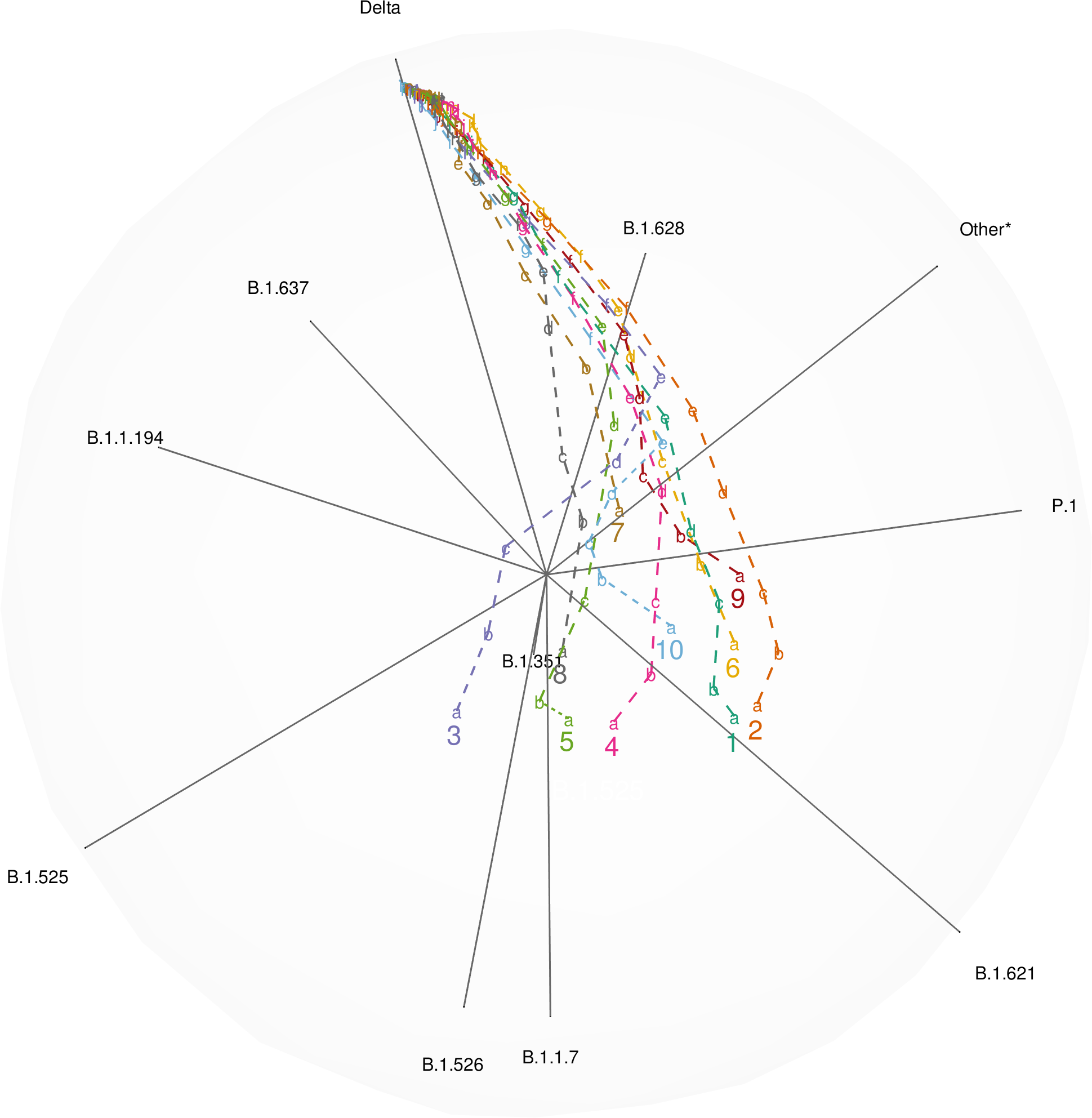
(a)

Variant Lineage	WHO Label
B.1.1.7	Alpha
B.1.351	Beta
P.1	Gamma
B.1.617.2, AY.1, AY.2	Delta
B.1.525	Eta
B.1.526	Iota
B.1.617.1	Kappa
B.1.621	Mu
B.1.628, B.1.637, B.1.1.194	Unassigned

(b)

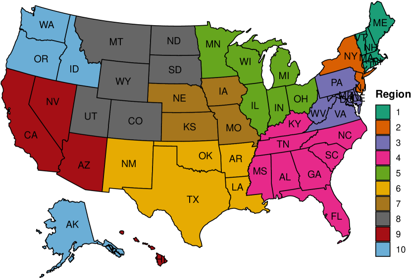
(c)

United States HHS Regions. (Note: Region 2 includes Puerto Rico and the Virgin Islands, while Region 9 includes American Samoa, Micronesia, Guam, Marshall Islands, Northern Marianas Islands and Palau.)

Figure 7: RadViz3D display of the SARS-Cov2 variant proportions (top right corner) over the summer of 2021 in the ten HHS regions of the US (indexed by map on bottom right corner). Half-broken lines connect the average variant proportions over the three weeks ending on (a) June 19, (b) June 26, (c) July 3, (d) July 10, (e) July 17, (f) July 24, (g) July 31, (h) August 7, (i) August 14, (j) August 21, (k) August 28, (l) September 4, (m) September 11 and (n) September 18.

The display demonstrates how the Delta variant rapidly eclipsed all SARS-Cov-2 infections across all ten HHS regions by the end of the time period. Our display shows the Delta variant with a notable head start in Region 7 where it was already the majority strain (65.9%) in the first time period under consideration. Delta also started with a weak majority (at 51.2%) in Region 8. The Alpha variant dominated most other regions in early June 2021; it is the majority variant in Regions 3–6 and 10. There was much greater diversity of strains during the dominance of Alpha in early June (time point (a) in Fig. 7a) compared to mid-September (time point (n)) during the dominance of Delta. Entropy varied from 0.90 in Region 7 to 1.67 in Region 1 in early June (0.75–1.49, excluding Delta), but decreased to a maximum across regions of 0.04 in Region 6 in mid-September. Despite the three-week averaging, there are fluctuations in variant compositions among time periods, especially in Regions 10 and (to a lesser extent) 3. The rapid fluctuations may be sampling error, but it is also evident that several variants were on the rise before Delta swept through. While Alpha monotonically declined, the next overall most prevalent variant Gamma peaked in weeks 2–3 in the northeast (Regions 1–3) and Region 8. The next most prevalent variant Mu (B.1.621) peaked east of the Mississippi (Regions 1–5) in weeks 2 and 3, in the west (Regions 9 and 10) in week 4 or 5, and displayed mixed behavior in the midwest (Regions 6–8). Other notable increases include a brief appearance of B.1.637 during weeks 2–4 in all regions but 7, B.1.628 increasing in all regions until about week 4 (July 10), with a slight two-week delay in Regions 7 and 8, and B.1.1.194 rising in prevalence in regions 3, 4, 9 and 10 in early June. These trends in the lesser variants likely explain why the trajectories do not simply traverse a straight line from Alpha to Delta, but veer toward P.1 (Gamma) or Mu (B.1.621), with nuances dictated by the mix of variants present in the HHS region at the start of the transition. We also caution that some of the patterns may be due to biases in variant sampling. It is plausible that patients with more severe disease, possibly Delta in particular, may seek medical care, increasing the chance of Delta inclusion in the surveillance sample, especially perhaps in regions with low testing rates. Regardless of the cause of the observed trends, RadViz3D very effectively illustrates the changing composition of the SARS-Cov-2 virus variants over the course of the summer of 2021.

IV Discussion

This short technical note shows that placement of anchor points in a radial visualization plot should ideally be as far away from each other as possible to avoid artificially-induced visual correlations between the coordinates. This desired property motivates our development of a fully 3D radial visualization tool called RadViz3D as it provides for larger distances between anchor points. Our development hinges on our exact and approximate solutions for the placement of $p$ anchor points on the 3D sphere. A R package radviz3d implementing our methodology is publicly available at https://radviz3d.github.io, and is demonstrated to accurately reveal class distinctions and lower-dimensional structure in simulated and standard classification datasets. As pointed out by a reviewer, the radial visualization methodology is naturally suited to displaying compositional data, so we have used RadViz3D to display to illustrate the historical development, by means of its chemical composition, of Longquan celadon and its Jingdezhen imitation. We also used the methodology to illustrate the changing face of the SARS-Cov-2 pandemic over the US regions during the summer of 2021.

Some aspects of our development could benefit from further attention. For instance, our development of RadViz3D demonstrates that we should use (at least approximately) equi-spaced anchor points, but the order of the anchor points may still be material. The order of anchor points corresponds to switching the order of the columns in the projection matrix $\bm{U}$ in (1). Clearly different orders of anchor points will produce different visualizations. For the visualization of grouped data, one possible solution to this is to run through all possible orders and pick one that has the biggest separation between groups, where $\ddot{\omega}$ can be used to measure separation. However, this would be very computationally demanding in higher dimensions. Also, based on our assumption that all coordinates are uncorrelated with equi-spaced anchor points, the order is intuitively perhaps not as important since all the coordinates are somewhat equivalent in our display. But it would still be worth getting a definitive answer. Further, for high-dimensional datasets, we will need to look at reducing dimensionality in data before using RadViz3D. [45] recently framed the grand tour [13, 14] in the context of radial visualization, with improvements for the “reverse curse of dimensionality” [46, 47, 48] or address data clumping or piling seen in the case of such displays with high-dimensional data, so it may be worth incorporating their ideas to potentially improve RadViz3D. Thus, we see that while this paper has made possible fully 3D radial visualization, there remain issues that merit additional investigation.

References

- [1] S. K. Card, J. D. Mackinlay, and B. Schneiderman, Readings in information visualization: using vision to think. Morgan Kaufmann, 1999.
- [2] E. Bertini, A. Tatu, and D. Keim, “Quality metrics in high-dimensional data visualization: an overview and systematization,” IEEE Transactions on Visualization and Computer Graphics, vol. 17, no. 12, p. 2203–2212, 2011.
- [3] A. Fonnet and Y. Prié, “Survey of immersive analytics,” IEEE Transactions on Visualization and Computer Graphics, vol. 27, no. 3, pp. 2101–2122, 2021.
- [4] J. M. Chambers, W. S. Cleveland, B. Kleiner, and P. A. Tukey, Graphical Methods for Data Analysis. Belmont, CA: Wadsworth, 1983.
- [5] H. Chernoff, “The use of faces to represent points in k-dimensional space graphically,” Journal of the American Statistical Association, vol. 68, no. 342, pp. 361–368, 1973.
- [6] A. Inselberg, “The plane with parallel coordinates,” The Visual Computer, vol. 1, pp. 69–91, 1985.
- [7] E. Wegman, “Hyperdimensional data analysis using parallel coordinates,” Journal of the American Statistical Association, vol. 85, pp. 664–675, 1990.
- [8] U. Fayyad, G. Grinstein, and A. Wierse, Information Visualization in Data Mining and Knowledge Discovery. Morgan Kaufmann, 2001.
- [9] D. F. Andrews, “Plots of high-dimensional data,” Biometrics, vol. 28, no. 1, pp. 125–136, 1972.
- [10] R. Khattree and D. N. Naik, “Andrews plots for multivariate data: Some new suggestions and applications,” Journal of Statistical Planning and Inference, vol. 100, no. 2, pp. 411–425, 2002.
- [11] K. R. Gabriel, “The biplot graphical display of matrices with application to principal component analysis,” Biometrika, vol. 58, pp. 453–467, 1971.
- [12] E. Kandogan, “Visualizing multi-dimensional clusters, trends, and outliers using star coordinates,” in Proceedings of the Seventh ACM SIGKDD International Conference on Knowledge Discovery and Data Mining, ser. KDD ’01. New York, NY, USA: ACM, 2001, pp. 107–116. [Online]. Available: http://doi.acm.org/10.1145/502512.502530
- [13] D. Asimov, “The grand tour: A tool for viewing multidimensional data,” SIAM Journal of Scientific and Statistical Computing, vol. 6, no. 1, pp. 128–143, 1985.
- [14] A. Buja, D. Cook, D. Asimov, and C. Hurley, “14 - computational methods for high-dimensional rotations in data visualization,” in Data Mining and Data Visualization, ser. Handbook of Statistics, C. Rao, E. Wegman, and J. Solka, Eds. Elsevier, 2005, vol. 24, pp. 391–413.
- [15] L. McInnes, J. Healy, N. Saul, and L. Grossberger, “Umap: Uniform manifold approximation and projection,” Journal of Open Source Software, vol. 3, p. 861, 09 2018.
- [16] P. Hoffman, G. Grinstein, K. Marx, I. Grosse, and E. Stanley, “DNA visual and analytic data mining,” in Proceedings of the 8th conference on Visualization ’97, VIS’97. IEEE Computer Society Press, 1997, p. 437–441.
- [17] P. Hoffman, G. Grinstein, and D. Pinkney, “Dimensional anchors: a graphic primitive for multidimensional multivariate information visualizations,” in Proceedings of the 1999 workshop on new paradigms in information visualization and manipulation in conjunction with the eighth ACM internation conference on Information and knowledge management. ACM, 1999, pp. 9–16.
- [18] G. G. Grinstein, C. B. Jessee, P. E. Hoffman, P. J. O’Neil, and A. G. Gee, “High-dimensional visualization support for data mining gene expression data,” in DNA Arrays: Technologies and Experimental Strategies, E. V. Grigorenko, Ed. Boca Raton, Florida: CRC Press LLC, 2001, ch. 6, pp. 86–131.
- [19] G. M. Draper, Y. Livnat, and R. F. Riesenfeld, “A survey of radial methods for information visualization,” IEEE Transactions on Visualization and Computer Graphics, vol. 15, no. 5, pp. 759–776, Sep. 2009.
- [20] A. O. Artero and M. C. F. de Oliveira, “Viz3d: effective exploratory visualization of large multidimensional data sets,” in Proceedings. 17th Brazilian Symposium on Computer Graphics and Image Processing, Oct 2004, pp. 340–347.
- [21] K. Daniels, G. Grinstein, A. Russell, and M. Glidden, “Properties of normalized radial visualizations,” Information Visualization, vol. 11, no. 4, pp. 273–300, 2012. [Online]. Available: https://doi.org/10.1177/1473871612439357
- [22] M. Ankerst, D. Keim, and H. P. Kriegel, “Circle segments: a technique for visually exploring large multidimensional data sets,” Human Factors, vol. 1501, pp. 5–8, 1996.
- [23] L. di Caro, V. Frias-Martinez, and E. Frias-Martinez, “Analyzing the role of dimension arrangement for data visualization in Radviz,” in Advances in Knowledge Discovery and Data Mining. Springer, 2010, p. 125–132.
- [24] J. Sharko, G. Grinstein, and K. A. Marx, “Vectorized Radviz and its application to multiple cluster datasets,” IEEE Transactions on Visualization and Computer Graphics, vol. 14, no. 6, pp. 1444–1451, December 2008.
- [25] T. van Long and V. T. Ngan, “An optimal radial layout for high dimensional data class visualization,” in 2015 International Conference on Advanced Technologies for Communications (ATC), 2015, pp. 343–346.
- [26] S. Cheng, W. Xu, and K. Mueller, “Radviz Deluxe: An attribute-aware display for multivariate data,” Processes, vol. 5, p. 75, 2017.
- [27] A. González, “Measurement of areas on a sphere using Fibonacci and latitude-longitude lattices,” Mathematical Geosciences, vol. 42, p. 49, january 2010.
- [28] M. Atiyah and P. Sutcliffe, “Polyhedra in physics, chemistry and geometry,” Milan Journal of Mathematics, vol. 71, no. 1, pp. 33–58, Sep 2003. [Online]. Available: https://doi.org/10.1007/s00032-003-0014-1
- [29] E. B. Saff and A. B. Kuijlaars, “Distributing many points on a sphere,” The Mathematical Intelligencer, vol. 19, pp. 5–11, dec 1997.
- [30] R. Maitra and V. Melnykov, “Simulating data to study performance of finite mixture modeling and clustering algorithms,” Journal of Computational and Graphical Statistics, vol. 19, no. 2, pp. 354–376, 2010.
- [31] V. Melnykov, W.-C. Chen, and R. Maitra, “MixSim: An R package for simulating data to study performance of clustering algorithms,” Journal of Statistical Software, vol. 51, no. 12, pp. 1–25, 2012. [Online]. Available: http://www.jstatsoft.org/v51/i12/
- [32] R Development Core Team, R: A Language and Environment for Statistical Computing, R Foundation for Statistical Computing, Vienna, Austria, 2018, ISBN 3-900051-07-0. [Online]. Available: http://www.R-project.org
- [33] V. Melnykov and R. Maitra, “CARP: Software for fishing out good clustering algorithms,” Journal of Machine Learning Research, vol. 12, pp. 69 – 73, 2011.
- [34] N. Campbell and R. Mahon, “A multivariate study of variation in two species of rock crab of the genus leptograpsus,” Australian Journal of Zoology, vol. 22, no. 3, pp. 417–425, 1974.
- [35] A. E. Raftery and N. Dean, “Variable selection for model-based clustering,” Journal of the American Statistical Association, vol. 101, pp. 168–178, 2006.
- [36] M. Forina, R. Leardi, and S. Lanteri, “PARVUS - an extendible package for data exploration, classification and correlation,” Via Brigata Salerno, 16147 Genoa, Italy, 1988.
- [37] M. Forina and E. Tiscornia, “Pattern recognition methods in the prediction of italian olive oil origin by their fatty acid content,” Annali di Chimica, vol. 72, pp. 143–155, 1982.
- [38] M. Forina, C. Armanino, S. Lanteri, and E. Tiscornia, “Classification of olive oils from their fatty acid composition,” in Food Research and Data Analysis. London: Applied Science Publishers, 1983, pp. 189–214.
- [39] I. A. Almodóvar-Rivera and R. Maitra, “Kernel-estimated nonparametric overlap-based syncytial clustering,” Journal of Machine Learning Research, vol. 21, no. 122, pp. 1–54, 2020.
- [40] A. D. Peterson, A. P. Ghosh, and R. Maitra, “Merging -means with hierarchical clustering for identifying general-shaped groups,” Stat, vol. 7, no. 1, p. e172, 2018.
- [41] G. S. G. M. Gompertz, Chinese Celadon Wares (Great Composers), 2nd ed. London: Faber and Faber, 1980.
- [42] M. Medley, The Chinese Potter: A Practical History of Chinese Ceramics, 3rd ed. London: Phaidon, 1989.
- [43] Z. He, M. Zhang, and H. Zhang, “Data-driven research on chemical features of jingdezhen and longquan celadon by energy dispersive x-ray fluorescence,” Ceramics International, vol. 42, 11 2015.
- [44] B. Peng, S. Zhou, Y. Shen, and B. Li, “EDXRF study on ming dynasty celadons’ sherds unearthed from longquan feng dong rock,” Journal of the Chinese Ceramic Society, vol. 11, no. 37, pp. 1904–1908, 2009.
- [45] U. Laa, D. Cook, and S. Lee, “Burning sage: Reversing the curse of dimensionality in the visualization of high-dimensional data,” Journal of Computational and Graphical Statistics, vol. 0, no. ja, pp. 1–19, 2021.
- [46] P. Diaconis and D. Freedman, “Asymptotics of Graphical Projection Pursuit,” The Annals of Statistics, vol. 12, no. 3, pp. 793 – 815, 1984.
- [47] J. S. Marron, M. J. Todd, and J. Ahn, “Distance-weighted discrimination,” Journal of the American Statistical Association, vol. 102, no. 480, pp. 1267–1271, 2007.
- [48] J. Ahn and J. S. Marron, “The maximal data piling direction for discrimination,” Biometrika, vol. 97, no. 1, pp. 254–259, 2010.