Abstract

We explore the alternatives for interrogating a fiber sensor from the polarization point of view, and demonstrate a better accuracy with dual polarization probing for coherent phi-OTDR compared with single polarization probing.

1 Introduction

Optical fiber sensors are becoming a hot topic as they enable distributed sensing over long distances and thus provide low cost, lightweight sensors. $\phi$-OTDR exploits the retro-propagated optical field induced by the Rayleigh backscattering effect in optical fibers,which is known to be polarization-dependent [1]. To overcome polarization fading effect, recent work focuses on the receiver design by using a dual-polarization coherent receiver [2, 3] so that the overall received optical power is kept constant. Relying on the same receiver configuration, [4] introduces optimized probing sequences of finite length that allow a mathematically perfect channel response estimation of the sensor array. Highly sensitive measurements using this probing technique are reported in [5].

As a matter of fact, the dual-polarization receiver setup is not sufficient to demonstrate a perfect channel estimation. The transmitter setup must as well be taken into account for a full understanding of a polarization insensitive sensor. Polarization-induced phase noise was observed and further analysed in [6]. This effect depends on the input state of polarization (SOP), unlike polarization fading that occurs when the receiver does not detect the full state of polarization information of the backscattered signal. In the following, we compare single and dual polarization interrogation schemes, considering Single (polarization) Input - Single (polarization) Output (SISO), Single Input - Multiple Output ($1\times 2$ SIMO) and Multiple Input - Multiple Output ($2\times 2$ MIMO) probing techniques, and investigate their respective issues. The study is performed using a dual-polarization backscattering model [7] and then validated by experimental results.

2 Polarization-sensitive sensing

The purpose of $\phi$-OTDR is to retrieve the backscattered phase evolution from the desired fiber segments, defined by a given spatial resolution (SR), itself defined by the interrogation rate used to probe the sensor. We use the probing technique [4] which consists in sending coded sequences either on one or two orthogonal polarization state(s). At the receiver side, we consider two schemes: coherent mixers with or without polarization diversity.

2.1 Phase estimation

• $2\times 2$ MIMO consists in sending and receiving on two orthogonal polarizations. It allows to recover the full Jones matrix of the channel $\textbf{H}=\begin{bmatrix}h_{xx}&&h_{xy}\\ h_{yx}&&h_{yy}\end{bmatrix}$ [4], where the matrix coefficients are complex numbers and describe the experienced polarization crosstalk in the channel. The estimated common phase is given by:

  $$\phi_{MIMO}=0.5\angle(\det{\textbf{H}})$$ (1)

• $1\times 2$ SIMO probes a single polarization, and uses a polarization diversity receiver. Signal is recovered on both polarizations, say, if the first column of H is sent: $\textbf{H'}=\begin{bmatrix}h_{xx}&&h_{yx}\end{bmatrix}^{T}$,

  $$\phi_{SIMO}=\angle(h_{xx}+h_{yx})$$ (2)

  Note that in (2) we also have $\phi_{SIMO}=\arctan(\dfrac{\Im_{xx}+\Im_{yx}}{\Re_{xx}+\Re_{yx}})$ with $\Re$, $\Im$ the real and imaginary parts of h data [2].
  

• SISO probes and recovers information on one polarization (say $X$). Estimated phase is $\phi_{SISO}=\angle(h_{xx})$.

As an event occurs along the sensor, phase variations appear in time, thus increasing the phase standard deviation locally. The main requirement for phase sensors is that no variation or “false alarm” occurs when the fiber is not disturbed (fiber said to be in “static mode”). The chosen metric for detection of events is the magnitude of phase standard deviation measured over the time dimension.

2.2 Fading and phase noise

In this section, a backscattering model from a single mode fiber (SMF) is defined for numerical simulations. Rayleigh backscatterers are randomly distributed along the fiber, and so is their reflectivity (backscattered intensity). The fiber is modeled as a succession of $N$ spatial segments $i\in[1,\texttt{N}]$, each of them defined by their round-trip Jones matrix $\textbf{H}_{i}$. The common phase factor and the total intensity of the reflected optical field are determined from the distribution and characteristics of the backscatterers per segment. For polarization evolution, we consider a random rotation along the segment [7]. For all segments $i$, $\textbf{H}_{i}$ is defined as the following:

$$\textbf{H}_{i}=A_{i}p_{i}\textbf{U}_{i}^{T}\textbf{M}\textbf{U}_{i}$$ (3)

where $\textbf{U}_{i}=\textbf{D}_{\beta_{i}}\textbf{R}_{\Theta_{i}}\textbf{D}_{\gamma_{i}}$ describes a general behaviour of forward transmission in the fiber segment: D are diagonal phase retarders and R is a polarization rotation real matrix, all of them unitary (of determinant 1 [8]). The parameters $\beta,\gamma$ are uniformly distributed over $[-\pi,\pi]$, and $\Theta_{i}=\arcsin{\sqrt{\xi_{i}}}$ with $\xi_{i}$ uniformly drawn in $[0,1]$. M is a reflection matrix, modeled here as a perfect reflection (no losses, no polarization transfers) $\textbf{M}=[\begin{smallmatrix}1&&0\\ 0&&-1\end{smallmatrix}]$, $A_{i}$ is the attenuation along the fiber, and $p_{i}$ is the common phasor of the matrix derived from the simulated positions of backscatterers in the fiber [7]. The general shape of the Jones backscatter matrix, is computed as follows for all spatial segments $i$:

$$\textbf{H}_{i}=A_{i}p_{i}\begin{bmatrix}e^{j2\gamma_{i}}(\cos 2\beta_{i}+j\sin 2\beta_{i}\cos 2\Theta_{i})&&-j\sin 2\beta_{i}\sin 2\Theta_{i}\\ -j\sin 2\beta_{i}\sin 2\Theta_{i}&&e^{-j2\gamma_{i}}(\cos 2\beta_{i}-j\sin 2\beta_{i}\cos 2\Theta_{i})\end{bmatrix}$$

Polarization fading occurs in interferometers when two interfering light waves get orthogonal SOP so no interference occurs and no sensor phase is measured. In SISO mode, if we detect $h_{xx}$, an intensity fading will occur for periodic $(\Theta,\beta)$ pairs where no phase estimation is available. Else, no fading is brought with either SIMO or MIMO methods, there will always be a phase estimation that is stable in time: $\varphi_{SIMO}=\angle(p_{i}\times(e^{j2\gamma_{i}}\cos 2\beta_{i}-j\sin 2\beta_{i}(e^{j2\gamma_{i}}\cos 2\Theta_{i}+\sin 2\Theta_{i})))$ and $\varphi_{MIMO}=\angle(p_{i})$. Of course, SIMO-estimated absolute phase differs from the real common phase due to rotations but, when sensing dynamic events, we are only intersted in phase variations and stability. Polarization diversity receivers have thus overcome this fading issue [3].

The dependence of $\varphi_{SIMO}$ on $\Theta,\beta,\gamma$ gives rise to so-called polarization induced phase noise. The measured sensor output phase depends on the input SOP [6], and the output SOP may vary due to the birefringence in the sensor. To capture the phenomenon in a more realistic way, we model a “TX/RX misalignment” acknowledging that a configuration where the input H and V polarizations at the transmitter are perfectly aligned with those of the receiver is very unlikely. We model the misalignment as a polarization rotation $\textbf{R}_{\theta}=\begin{bmatrix}cos{\theta}&&-sin{\theta}\\ sin{\theta}&&cos{\theta}\end{bmatrix}$. Then $\textbf{H}_{i}$ becomes, for any spatial segment $i$, $\textbf{H}_{i}=A_{i}p_{i}\textbf{U}_{i}^{T}\textbf{M}\textbf{U}_{i}\textbf{R}_{\theta}$. Note that the input SOP includes possible mechanical perturbations around the setup, so $\theta$ (then $\textbf{R}_{\theta}$) can be time-dependent.

3 Polarization noise simulations

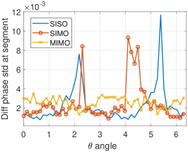
(a) StDv in time as a function of $\theta$, estimation on one segment, fixed $\Theta,\beta,\gamma$

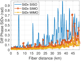
(b) StDv in time as a function of fiber length, randomly drawn $\Theta,\beta,\theta,\gamma$ for each segment

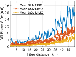
(c) Mean StDv over 50 fibre simulations

Fig. 1: Standard deviation of differential phase in $\theta$ and distance, $\Delta\nu$=75Hz

We simulate Rayleigh backscattering through a fiber with a given laser phase noise due to a laser linewidth $\Delta\nu$ [7], and observe the polarization effects on phase standard deviation in time (StDv) per fiber segment, within a time window of a few seconds, with a new phase estimation derived each 160 $\mu$s. For a given random $\Theta$, some input $\theta$ may lead to higher phase variations when single-input probing techniques are used, as shown in Fig.1a. As a result, this affects the phase StDv as a function of distance (Fig.1b), where SIMO method experiences sudden variations at random fiber distances, ie. at random segment indices. These variations correspond to occurrences of ($\Theta$, $\theta$) pairs where the impact of input polarization induced phase noise is visible. SISO-estimated phase cumulates this effect with polarization fading due to the varying birefringence in the fiber, leading to higher values of standard deviation spread along the simulated fiber. MIMO probing is independent of $\theta$ and thus yields no StDv peaks along the fiber. Fig.1c highlights that on average, there is a clear hierarchy between the three studied probing methods. Particularly on long distances: after 50km, the phase noise StDv given by MIMO probing is twice smaller than the one with SIMO probing, and five times smaller than SISO.

Back to a SIMO configuration, we choose fixed $\theta$ (polarization misalignment on the transmitter side) and $(\beta,\gamma)$ (phase retardances) to follow real (denoted $\Re$) and imaginary (denoted $\Im$) parts of $h_{xx}+h_{yx}$ for different $\Theta$ (polarization rotation in a fiber segment) in Figure 2. The standard deviation of the phase $\angle(h_{xx}+h_{yx})$ for that segment is superimposed. As SIMO-estimated phase is a modulation of the common phasor $p_{i}$ by the polarization parameters $\Theta,\beta$ and $\gamma$ (polarization phase noise) of the fiber segment as follows : $\varphi_{SIMO}=\angle(p_{i}\times(e^{j2\gamma_{i}}\cos 2\beta_{i}-j\sin 2\beta_{i}(e^{j2\gamma_{i}}\cos 2\Theta_{i}+\sin 2\Theta_{i})))$, we expect the $\Re$ and $\Im$ parts to be modulated as a function of $\Theta$.

Fig. 2: Periodicity of $\Im(h_{xx}+h_{yx})$, $\Re(h_{xx}+h_{yx})$ and StDv over $\Theta$ (SIMO interrogation, for given $\gamma$, $\beta$, $\theta$)

That modulation as a function of $\Theta$ not only changes the value of the phase estimation ($\Im$ part), but also yields phase StDv peaks when $\Re(h_{xx}+h_{yx})$ is close to zero, inducing a fading effect. As this “input polarization fading” occurs periodically as a function of $\Theta$ (as well as $\gamma$ and $\beta$, not displayed for simplicity) in the fibre and since there are no means for controlling such an intrinsic parameter of the fiber sensor, SIMO interrogation method is thus limited by polarization-induced phase noise, even though we should be capable of retrieving a phase at all times from a polarization insensitive receiver. In non-coherent interferometric setups, polarization induced phase noise appears as phase fluctuations and thus visibility fluctuations at the receiver side [6]. In that case, the standard solution to overcome this issue is to use depolarized light at the transmitter. We investigate here an alternate solution, based on joint probing of two polarizations: MIMO probing method is immune to polarization phase noise, thus experiences potential phase StDv peaks only when the backscattered intensity of a segment is low.

4 Experimental validation

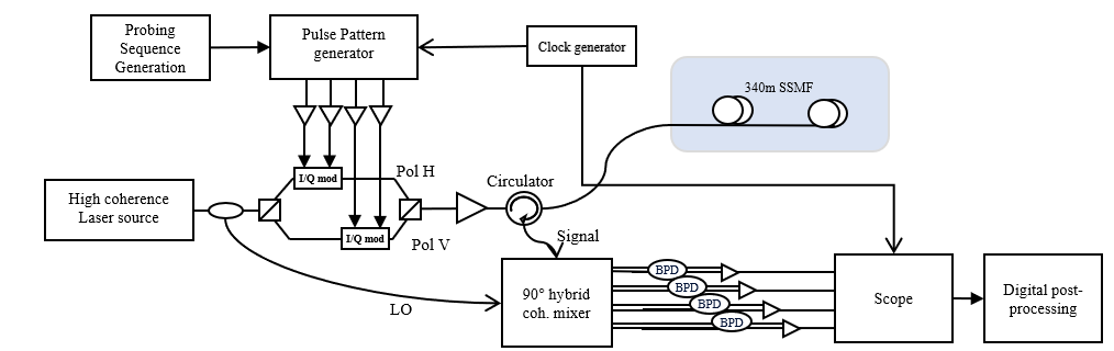
Fig. 3: Experimental setup

We perform measurements on a 340m-long standard single mode fiber (SSMF). The fiber experiences no strain so to stay in “static” conditions, as it was for the simulations. The experimental setup is shown in Figure 3. Both measurements couldn’t be performed simultaneously but were made successively so to keep the same/closest as possible conditions for the setup. For the SIMO measurement, the modulator modulates complementary binary sequences on one polarization only. Then, the second polarization is modulated too, with orthogonal sequences, and the MIMO measurement is performed. The measured standard deviation (StDv) of the phase is plotted Figure 4. We observe StDv peaks for both SIMO and MIMO probing due to low backscattered power from the fiber segments. The peaks are not perfectly aligned due to mere synchronization issues. Both StDv are low since no perturbation is applied to the sensing fiber, however we observe a high number of StDv peaks for SIMO whereas MIMO has only two (attributed to low intensity backscatter). The experimental result shows a better phase stability using MIMO probing, thus confirming our modeling results.

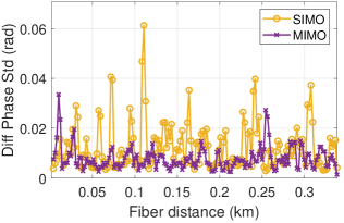
Fig. 4: SIMO and MIMO optical phase standard deviations as a function of fiber length, 340m SSMF

5 Conclusions

We pointed out the existence of two different polarization-related impairments in interferometric sensors and observed their influence through simulations. Simulation allowed to isolate some effects so to separate the contribution of independent disturbances which usually occur together in experimental setups. This study allows to claim that the presence of a polarization diversity receiver or any other technique to mitigate polarization fading is a necessary condition but not sufficient to overcome all polarization effects occurring along the sensor. Dual-polarization probing of the fiber sensor makes it insensitive to the input polarization fluctuation effects, thus dividing the phase noise by two on long distances. It appears as a promising complement to the polarization diversity receiver in a coherent-$\phi$-OTDR setup.

References

- [1] M. O. V. Deventer, “Polarization properties of rayleigh backscattering in single-mode fibers,” Journal of Lightwave Technology 11, 1895–1899 (1993).
- [2] Q. Yan, M. Tian, X. Li, Q. Yang, and Y. Xu, “Coherent -OTDR based on polarization-diversity integrated coherent receiver and heterodyne detection,” in “2017 25th Optical Fiber Sensors Conference (OFS),” (2017), pp. 1–4.
- [3] H. F. Martins, K. Shi, B. C. Thomsen, S. Martin-Lopez, M. Gonzalez-Herraez, and S. J. Savory, “Real time dynamic strain monitoring of optical links using the backreflection of live PSK data,” Optics Express 24, 22303 (2016).
- [4] C. Dorize and E. Awwad, “Enhancing the performance of coherent OTDR systems with polarization diversity complementary codes,” Opt. Express 26, 12878–12890 (2018).
- [5] C. Dorize, E. Awwad, and J. Renaudier, “High sensitivity -OTDR over long distance with polarization multiplexed codes,” IEEE Photonics Technology Letters 31, 1654–1657 (2019).
- [6] A. D. Kersey, M. J. Marrone, and A. Dandridge, “Analysis of input-polarization-induced phase noise in interferometric fiber-optic sensors and its reduction using polarization scrambling,” Journal of Lightwave Technology 8, 838–845 (1990).
- [7] S. Guerrier, C. Dorize, E. Awwad, and J. Renaudier, “A dual-polarization rayleigh backscatter model for phase-sensitive OTDR applications,” in “Optical Sensors and Sensing Congress,” (OSA, 2019), p. ETu3A.4.
- [8] J. N. Damask, Polarization optics in telecommunications, vol. 101 (Springer Science & Business Media, 2004).