Higher-order QCD corrections to $H\to b\bar{b}$ from rational approximants

Abstract

We use rational approximants to study missing higher orders in the massless scalar-current quark correlator. We predict the yet unknown six-loop coefficient of its imaginary part, related to $\Gamma(H\to b\bar{b})$, to be $c_{5}=-6900\pm 1400$. With this result, the perturbative series becomes almost insensitive to renormalization scale variations and the intrinsic QCD truncation uncertainty is tiny. This confirms the expectation that higher-order loop computations for this quantity will not be required in the foreseeable future, as the uncertainty in $\Gamma(H\to b\bar{b})$ will remain largely dominated by the Standard Model parameters.

1 Introduction

Without direct evidence for new physics from the Large Hadron Collider (LHC), searches for physics beyond the Standard Model will rely, in the near future, on indirect evidence from precise measurements that could reveal small deviations from the Standard Model (SM) predictions. Higgs physics plays a central role in this program. So far, the LHC has not found any statistically significant evidence of deviations from SM expectations in this sector, but the uncertainties in measurements of the required cross-sections and decay rates, for example, remain rather significant. With future facilities, such as the FCC-ee [1], which is planned to run as a Higgs factory at $\sqrt{s}=250$ GeV, the experimental status should improve dramatically. This will require a large effort on the theory side to reach the required precision for these processes [2, 3], lest the tests of the SM remain inconclusive.

The dominant decay channel for the SM Higgs boson is in a $b\bar{b}$ pair. At the LHC, however, due to the contamination from the hadronic background, the measurement of the decay $H\to b\bar{b}$ is challenging and the first results were reported only in 2018 [4, 5]. The precise description of this decay in the SM requires the calculation of higher-order perturbative QCD contributions, which are the dominant source of radiative corrections. The result is known with full quark-mass dependence at NLO [6, 7] and at order $\alpha_{s}^{2}$ from Ref. [8]. Beyond NNLO, quark-mass effects are treated perturbatively, with the leading order results obtained for massless bottom quarks (in the quark propagators), receiving small $m_{b}/m_{H}$ corrections (top mass effects, on the other hand, can be sizeable). In this framework, the corrections in the limit $m_{b}/m_{H}\to 0$ are completely known up to $\alpha_{s}^{4}$ thanks to the impressive five-loop computation of the terms originating from the Higgs-bottom Yukawa coupling [9, 10] and the work of Ref. [11] where the top-quark induced terms are calculated in the effective field theory framework, with the top quark integrated out. (A complete discussion of further corrections, electroweak and mixed electroweak for example, can be found in the dedicated reviews such as Ref. [12].)

In this work, we are concerned with estimating higher orders in the Higgs-bottom Yukawa induced contributions in the massless limit, starting at N5LO, or six loops, which may never be calculated exactly, with the aim of reassessing the intrinsic truncation error associated with perturbative QCD. We will employ different types of rational approximants, or Padé approximants [13, 14], in order to exploit the exact knowledge of the first four terms in the perturbative series to reconstruct the series to even higher orders. Variants of this method have been used for a long time, in different processes. Here, our strategy follows what was developed for hadronic $\tau$ decays [15], where the QCD corrections, arising from the massless Adler function, are also known up to $\mathcal{O}(\alpha_{s}^{4})$ (N4LO) [16, 10]. Ref. [15] is the main reference of the present work.

The strategy can be summarized as follows. First, we make use of the results for the relevant correlator in the large-$\beta_{0}$ limit of QCD [17, 18, 19], which provides an all-order realistic series, with renormalon singularities and the associated factorial divergences, in which different approximants can be tested and their precision can be judged by comparison with the exact results. In fact, we will exploit mainly rational approximants built to the Borel transform of the perturbative series, since this transform suppresses the factorial divergences and can have a finite radius of convergence. This type of method is sometimes referred to as “Padé-Borel” and benefits from the fact that rational approximants are ideal to approximate functions with isolated poles — here those poles are the renormalons of perturbation theory. Using the results from the large-$\beta_{0}$ limit, we are able to design the ideal strategy to the problem at hand. This strategy is then employed in full QCD, where our knowledge is limited to the first four non-trivial coefficients of the series.

We will show that the so-called D-log Padé approximants play a central role in our analysis. This type of approximant, which is less common in the literature, is particularly suitable to deal with functions containing branch points or poles with higher multiplicity. In QCD, the renormalon poles evolve into branch points [19, 20], which is precisely why D-log Padés are so appealing when working with the Borel transformed perturbative series.

Through a careful and systematic use of these rational approximants, we are able to obtain a model-independent prediction for the first unknown coefficient of the scalar $q\bar{q}$ correlator, the $\alpha_{s}^{5}$ term (N5LO), with an associated uncertainty — a benefit of our method. We also obtain estimates for even higher orders, starting at N6LO, albeit with an increasingly large error. With these results we can calculate the total perturbative QCD contribution to the decay width of the Higgs boson into $b\bar{b}$ with an associated uncertainty for missing higher orders. The use of our results for the N5LO coefficient further decreases the perturbative uncertainty. Our results confirm the expectation that the dominant QCD contributions arising from the scalar $q\bar{q}$ correlator are under very good control, with a small error from the truncation of the series, and they reinforce that the major limiting factors for this decay are, and will be in the foreseeable future, the precision of the $b$-quark mass and of the strong coupling.

This paper is organized as follows. We start in Sec. 2 with a brief overview of elements of Padé theory with focus on our applications. In Sec. 3 we define the massless scalar correlator and related physical observables and present their perturbative expansion up to the last known term, the $\mathcal{O}(\alpha_{s}^{4})$. In Sec. 4 we discuss in detail a specific application in the large-$\beta_{0}$ limit, which serves as a proof of concept. In Sec. 5, we present our results in QCD and their impact on the decay width for $H\to b\bar{b}$. Our conclusions are given in Sec. 6.

2 Padé approximants in a nutshell

In this section we give an overview of the most important concepts about Padé approximants and their variants that are used in the presented work. A more detailed discussion focussed on a similar application can be found in Ref. [15]; broader reviews of the topic can be found in Refs. [13, 14, 21].

Let us consider a function $f(z)$ whose series expansion in the complex plane around $z=0$ is given by

$$f(z)=\sum_{n=0}^{\infty}f_{n}z^{n}.$$ (1)

A Padé approximant to the function $f(z)$ [14], denoted as $P_{N}^{M}(z)$, is defined as the ratio of two polynomials $Q_{M}(z)$ and $R_{N}(z)$ of order $M$ and $N$ respectively, where the definition $R_{N}(0)=1$ is employed without loss of generality

$$P_{N}^{M}(z)=\dfrac{Q_{M}(z)}{R_{N}(z)}=\dfrac{a_{0}+a_{1}z+\cdots+a_{M}z^{M}}{1+b_{1}z+\cdots+b_{N}z^{N}}.$$ (2)

The PA makes a “contact” of order $M+N$ with the expansion of the function around $z=0$ [22]; which means that, when $P_{N}^{M}(z)$ is expanded around this point, it will reproduce exactly the first $M+N+1$ coefficients $f_{n}$, thus returning values for $a_{0},...,a_{M}$, and $b_{1}$,…,$b_{N}$ and predicting the coefficients of order higher than $M+N$.

In the Padé approximant theory, Pomerenke’s theorem guarantees the convergence of Padés sequences $P^{N+k}_{N}$, for $k\geq-1$, to the original function, as long as $f(z)$ is meromorphic, either being Stieltjes or not [22, 23, 24]. Accordingly, these Padés are convergent everywhere in any compact set of the complex plane, excluding a set of zero area which contains the poles of the original function [14]. The sequence of PAs reproduces the analytic structure of $f(z)$, its poles and residues, in a hierarchical fashion: poles that lie closer to the origin will be well reproduced already at lower orders, while poles (and the associated residues) that are further away from the origin will not correspond to any singularity of the original function, and can only be considered as effective poles. In the process, extraneous poles can be generated, but the theorem also ensures that, in any compact region in the complex plane, these poles of the PAs will move far from this region when the order of the PA is increased or they will appear in combination with near-by zeros of the numerator $Q_{M}(z)$, constituting what is known as defects or Froissart doublets. These defects play an important role in the analysis of the convergence of the series of PAs, since they entail a cancellation which effectively reduce the order of the PA.

For meromorphic functions, some of the poles and residues of the PA may be complex, even if the original function does not have complex poles [22, 23, 24]. These poles of the PA cannot be identified with any singularity of the original function, but it remains possible to employ those Padés to study the function away from the complex poles. However, in their vicinity the Padé approximation deteriorates. These complex poles are transient: they appear and disappear when the order of the Padé is raised [22, 23, 24].

In the problem we are dealing with, the Borel transform in the large-$\beta_{0}$ limit contains only isolated renormalon poles. However, the singularities of the Borel transform of the perturbative series in full QCD become superimposed cuts instead of isolated poles. Although there are no convergence theorems in Padé theory for generic functions with cuts (except for Stieltjes functions) experience shows that PAs can approximate functions with cuts remarkably well. This is achieved by an accumulation of poles along the cut, which mimics the singularity structure of the original function [14, 21].

A different kind of PAs that is very useful for functions with branch points or poles with higher multiplicity are the D-log Padé approximants [14, 15]. Let us consider the function

$$f(z)=A(z)\,\dfrac{1}{(\mu-z)^{\gamma}}+B(z),$$ (3)

where $A(z)$ and $B(z)$ are functions with little structure and analytic at $z=\mu$. We are primarily interested in the case in which $f(z)$ has a branch point at $z=\mu$, and accordingly $\gamma$ is a non-integer number, but in reality this condition is not essential. We can define now a new function $F(z)$ near $z=\mu$ as [14]

$$F(z)=\dfrac{\mathrm{d}}{\mathrm{d}z}\ln{f(z)}\approx\dfrac{\gamma}{(\mu-z)}.$$ (4)

The function $F(z)$ has a simple pole and the residue is the exponent of the cut of $f(z)$. Thus, with $\bar{P}_{N}^{M}(z)$ being the Padé constructed to $F(z)$ defined above, the D-log Padé, $\mathrm{Dlog}_{N}^{M}(z)$, of $f(z)$ is given by the expression below [14, 15]

$$\mathrm{Dlog}_{N}^{M}(z)=f(0)\exp{\left[\int\mathrm{d}z\,\bar{P}_{N}^{M}(z)\right]}.$$ (5)

Because of the derivative in Eq. 4, the $f(0)$ term is lost and must be reintroduced in order to correctly normalize the D-log Padé. The $\mathrm{Dlog}_{N}^{M}$ then reproduces exactly the first $M+N+2$ coefficients of $f(z)$ (one order more than the usual $P_{N}^{M}$) and can be used to predict the $(M+N+3)$-th coefficient and higher. The D-log Padé is no longer a rational approximant, however the function $F(z)$ is meromorphic and, because of that, it is easily approximated by the Padé $\bar{P}_{N}^{M}$.

In principle, this type of approximant offers a way to determine the branch point and the exponent of the cut of the original function $f(z)$ from the study of the PA to $F(z)$ around its pole. Since no assumption about $\mu$ or $\gamma$ is made, their estimates are exclusively obtained from the series coefficients.

3 Scalar correlator

As already mentioned, the decay width of the Higgs boson into the pair $b\bar{b}$ is known up to fourth order in QCD [9, 10] in the massless limit and is related to the imaginary part of the quark-antiquark scalar current correlator. This correlator, that is not directly associated with any physical quantity, is defined as

$$\Pi(p^{2})\equiv i\int\mathrm{d}x\,\mathrm{e}^{ipx}\,\langle\Omega|T\{j(x)j^{\dagger}(0)\}|\Omega\rangle,$$ (6)

with $|\Omega\rangle$ representing the non-perturbative QCD vacuum. The scalar current $j(x)$ arises from the interaction between the Higgs and the bottom quarks and is given by

$$j(x)=m_{q}\,\overline{q}_{f}(x)q_{f}(x),$$ (7)

where $q(x)$ is the quark field treated as massless in loop calculations. The mass of the quark, $m_{q}$, is introduced to ensure renormalization group invariance for the physical observables.

The purely perturbative expansion of $\Pi(s)$ in powers of the strong coupling is given by the following general form [25]

$$\Pi(s)=-\dfrac{N_{c}}{8\pi^{2}}\,s\,m_{q}^{2}(\mu)\sum_{n=0}^{\infty}a_{s}^{n}(\mu)\sum_{k=0}^{n+1}d_{n,k}L^{k},$$ (8)

where $s\equiv p^{2}$. The quark mass $m_{q}$ and the QCD coupling $a_{s}\equiv\alpha_{s}/\pi$, both in the ${\overline{\rm MS}}$ scheme, are renormalized at the scale $\mu$, which appears in the logarithms $L\equiv\ln{(-s/\mu^{2})}$ as well. Setting the scale $\mu^{2}=-s$ the logarithms are resummed.

The coefficients $d_{n,0}$ depend on the conventions related to the renormalization procedure and do not contribute in any physical quantity. Furthermore, the coefficients $d_{n,k}$, with $k>1$, can be obtained from the RGE of the scalar correlator [26]. Hence the only independent coefficients for each perturbative order are $d_{n,1}$, which are known analytically up to fourth order and whose numerical values for five active flavours, $N_{f}=5$, and $N_{c}=3$ are [9, 10]

$$d_{1,1}=5.6667,\qquad d_{2,1}=42.032,\qquad d_{3,1}=353.229,\qquad d_{4,1}=3512.2.$$ (9)

The physical decay width for $H\to b\bar{b}$ is related to the imaginary part of the scalar correlator $\Pi(s)$ as

$$\Gamma\left(H\rightarrow b\bar{b}\right)=\dfrac{1}{m_{H}\,v^{2}}\,\operatorname{Im}\Pi(s),$$ (10)

where $v^{2}$ is the Higgs vacuum expectation value. Setting the renormalization scale to $\mu^{2}=s\equiv m_{H}^{2}$, so that the logarithms are summed, the general perturbative expansion for the imaginary part of $\Pi(s)$ is

$$\operatorname{Im}\Pi(s)=\dfrac{N_{c}}{8\pi}\,m_{q}^{2}(m_{H})\,s\sum_{n=0}^{\infty}a_{s}^{n}(m_{H})\sum_{k=0}^{[n/2]}d_{n,2k+1}(i\pi)^{2k},$$ (11)

with $[x]$ representing the integer part of $x$. For $N_{f}=5$, the expansion which is known up to fourth order in QCD is

$$\operatorname{Im}\Pi(s)=\dfrac{N_{c}}{8\pi}\,m^{2}_{q}(m_{H})\,s\left[1+\sum_{n=1}^{\infty}c_{n}a_{s}^{n}\right]=\dfrac{N_{c}}{8\pi}\,m^{2}_{q}(m_{H})\,s\left[1+F(a_{s})\right]$$

$$=\dfrac{N_{c}}{8\pi}\,m^{2}_{q}(m_{H})\,s\left[1+5.6667\,a_{s}+29.1467\,a_{s}^{2}+41.7576\,a_{s}^{3}-825.747\,a_{s}^{4}+\dots\right].$$ (12)

In passing, we defined the function $F(a_{s})$ which contains the $\alpha_{s}$ corrections to $\operatorname{Im}\Pi(s)$ and is referred to as the reduced imaginary part. As seen above, a negative coefficient appears in the term of order $a_{s}^{4}$ of the imaginary part of $\Pi(s)$. Since the imaginary part of the scalar correlator is a physical observable, it satisfies a homogeneous RGE and the logarithms can be reinstated from the expressions above.

Another renormalization group invariant quantity is the second derivative of the scalar correlator with respect to $s$ [25, 20], which removes the two scheme-dependent subtraction constants. Its general perturbative expansion can be easily obtained from Eq. (8) and, resumming the logarithms with the scale $\mu^{2}=-s$, we have [25]

$$\Pi^{\prime\prime}(s)=-\dfrac{N_{c}}{8\pi^{2}}\dfrac{m^{2}_{q}(m_{H})}{s}\left[1+\sum_{n=1}^{\infty}r_{n}a_{s}^{n}\right],$$ (13)

where $r_{n}=\left(d_{n,1}+2d_{n,2}\right)$ and whose numerical coefficients for $N_{f}=5$ are

$$\Pi^{\prime\prime}(s)=-\dfrac{N_{c}}{8\pi^{2}}\dfrac{m^{2}_{q}(m_{H})}{s}\left[1+3.6667\,a_{s}+12.8098\,a_{s}^{2}+39.6839\,a_{s}^{3}+153.955\,a_{s}^{4}+\dots\right].$$ (14)

Since all the series discussed here are (at best) asymptotic, it is convenient to work with their Borel transform, which suppresses the factorial divergence of the series coefficients. Without loss of generality, we always consider the Borel transform of functions starting at $\mathcal{O}(\alpha_{s})$, such as $F(a_{s})$ in Eq. (12). We refer to these functions as “reduced functions”. Let

$$R(\alpha_{s})=\sum_{k=0}^{\infty}r_{k}\,\alpha_{s}^{k+1},$$ (15)

be an asymptotic expansion of a given observable $R$. We define its Borel transform as

$$B[R](u)=\sum_{k=0}^{\infty}\dfrac{r_{k}}{k!}\left(\frac{2\pi}{\beta_{1}}\right)^{k+1}\,u^{k},$$ (16)

where $\beta_{1}$ is the first coefficient of the QCD $\beta$ function (see App. A). The Borel integral, which gives the value of $R$ summed in the Borel sense (provided the integral exists), is

$$R=\int\displaylimits_{0}^{\infty}{\rm d}u\,\mathrm{e}^{-2\pi u/(\beta_{1}\alpha_{s})}B[R](u).$$ (17)

The singularities of the Borel transform in the complex $u$ plane, which in our case are the renormalons of perturbation theory, govern the behavior of the perturbative series at intermediate and higher orders [19]. Poles on the negative real axis generate sign alternating coefficients. These poles are of UV origin in the applications we discuss in this paper. Poles of IR origin are located on the positive real axis and obstruct the integration in Eq. (17). A prescription to circumvent these poles must be adopted, which generates an imaginary ambiguity in the Borel sum of the series. It is expected on general grounds that these ambiguities cancel against the non-perturbative corrections from higher-dimensional OPE condensates. In the presence of several renormalon singularities, the one closest to the origin dominates the series behavior at intermediate and large orders.

In this work, in the majority of cases, we will build PAs to the Borel transforms of the series in $\alpha_{s}$. This procedure, sometimes referred to as Padé-Borel approximants, is known empirically to lead to faster convergence [27] for asymptotic series of the type we have here (see Ref. [28] and references therein).

4 A proof of concept in the large-$\beta_{0}$ limit

The aim of this section is to employ our technique in a realistic case, as a proof of concept of our method. We choose to highlight an application of D-log Padé approximants, since these are very seldom used in the literature. We apply them to the Borel transform of $\Pi^{\prime\prime}(s)$ in the large-$\beta_{0}$ limit of QCD [17, 18]. We choose to work initially in this limit because it provides an entirely consistent simplified model where higher-order corrections are known to all orders in the coupling. The series exhibit the renormalon divergences, although they appear as simple or double poles (and not branch cuts as in full QCD) [19]. The large-$\beta_{0}$ result is obtained from the leading $N_{f}$ terms, which can be calculated for the scalar correlator by considering light-quark bubble loop corrections to the gluon propagators in the 2-loop result. Then, through the procedure known as naive non-abelianization [18, 17], in which the fermionic contribution to the QCD beta function is replaced by the full one-loop beta function coefficient ($\beta_{1}$ in our notation), a set of non-abelian terms is effectively introduced, generating a realistic result to all orders in $\alpha_{s}$.

The massless scalar correlator in the large-$\beta_{0}$ limit was first calculated by Broadhurst, Kataev and Maxwell [29], who obtained a result for its Borel transform in closed form. With this result and the recent discussion in Ref. [25] one finds that the Borel transform of $\operatorname{Im}\Pi(s)$, in terms of the renormalization group invariant (RGI) quark mass (see App. A), can be written as

$$B[\widehat{F}^{C}_{L\beta}](u)=\dfrac{3C_{F}}{\beta_{1}}\left[\dfrac{\sin{\pi u}}{\pi u}\left[1+u\,G_{D}(u)\right]\mathrm{e}^{(C+5/3)u}-1\right]\dfrac{1}{u},$$ (18)

where $C_{F}=4/3$ and $C$ is a parameter that controls the renormalization scheme, with $C=0$ corresponding to ${\overline{\rm MS}}$, our preferred choice. The function $G_{D}(u)$ can be written as

$$G_{D}(u)=\dfrac{2}{1-u}-\dfrac{1}{2-u}+\dfrac{2}{3}\sum_{k=3}^{\infty}\dfrac{(-1)^{k}}{(k-u)^{2}}-\dfrac{2}{3}\sum_{k=1}^{\infty}\dfrac{(-1)^{k}}{(k+u)^{2}}.$$ (19)

Due to the zeros of the function $\frac{\sin{\pi u}}{\pi u}$, the Borel transform (18) has no renormalons in $u=1$ and $u=2$ and all poles are simple poles. (Note that the expression is regular at $u=0$.)

The Borel transform of the reduced second derivative of $\Pi(s)$ written in terms of the RGI quark mass in large-$\beta_{0}$ is

$$B[\widehat{D}_{L\beta}^{C}](u)=\dfrac{3C_{F}}{\beta_{1}}\left[(1-u)\left[1+u\,G_{D}(u)\right]\mathrm{e}^{(C+5/3)u}-1\right]\dfrac{1}{u}.$$ (20)

This Borel transform has a simple IR pole at $u=2$, associated with the gluon condensate corrections. The other renormalon poles, at $u=-1,-2,-3,\dots$ and $u=3,4,5,\dots$, are all double poles. Since the second derivative of the scalar correlator is physical, there is no renormalon at $u=1$. At sufficiently high orders the perturbative series coefficients will be dominated by the UV pole at $u=-1$, which is the pole closest to the origin, and will be sign alternating.

Comparing the Borel transforms of $\operatorname{Im}\Pi(s)$ and $\Pi^{\prime\prime}(s)$ one sees that in the first the double poles are reduced to simple poles, which should improve the performance of the PAs. However, this is done at a price: the PA will need to reproduce the function $\sin(\pi u)$ as well. In this scenario, it is advantageous to work with the Borel transform of $\Pi^{\prime\prime}(s)$ but using D-log Padé approximants, which achieve the reduction of the double poles to simple ones without the complications of the prefactor of Eq. (18). We focus on this case.

Reconstructing the perturbative expansion of $\widehat{D}_{L\beta}^{C}$ in the ${\overline{\rm MS}}$ scheme with $N_{f}=5$ we find

$$\widehat{D}_{L\beta}=5.3333\,a_{s}+6.0111\,a_{s}^{2}+42.8911\,a_{s}^{3}+0.7729\,a_{s}^{4}+1512.48\,a_{s}^{5}-8410.57\,a_{s}^{6}+\dots.$$ (21)

The coefficients of Eq. (21) should not be directly compared with those of Eq. (14), since here we are expressing the result in terms of $\widehat{m}_{q}$. The expected sign alternation of the coefficients, dictated by the UV renormalon, sets in from the sixth-order coefficient onwards.

4.1 D-log Padé approximants

One could build standard PAs to the Borel transform of Eq. (20). Although these approximants do display convergence, they are not optimal and the convergence of the procedure can be accelerated with the use of D-log Padé approximants. One of the reasons for the slower convergence of the PAs in the case of the Borel transform of $\Pi^{\prime\prime}(s)$ is the presence of an infinite number of double poles. Ideally, the approximants need to reproduce the pole multiplicity in order to achieve a good description of the series, which requires a larger number of input coefficients. A method that can be more effective in the presence of multiple poles are the D-log Padés defined in Sec. 2. We now turn to their application in approximating the Borel transform of the series $\widehat{D}_{L\beta}$, given in Eq. 20.

We remind that the D-log Padé $\mathrm{Dlog}_{N}^{M}$ is built from a PA $\bar{P}_{N}^{M}$ to the function $F(z)$ of Eq. (4). It reproduces the first $N+M+2$ coefficients and can be used to predict the $(M+N+3)$-th coefficient and higher. We will consider $\mathrm{Dlog}_{N}^{M}(u)$ with $N+M=2$ or higher, since otherwise the PAs $\bar{P}_{N}^{M}$ that are required contain too little information (one or two coefficients only). The perturbative coefficients predicted by the D-log Padés will be denoted $\widehat{r}_{k}^{P}$ and are the counterpart of the exact coefficients of Eq. (21), denoted by $\widehat{r}_{n}$. We assess the convergence of the D-log Padé sequence through the relative error of the predicted coefficients, defined as

$$\sigma_{\mathrm{rel}}=\left\lvert\dfrac{\widehat{r}^{P}_{n}-\widehat{r}_{n}}{\widehat{r}_{n}}\right\rvert.$$ (22)

Let us begin examining a simple example, $\mathrm{Dlog}_{1}^{1}(u)$, whose expression is

$$\mathrm{Dlog}_{1}^{1}(u)=\dfrac{64}{23}\dfrac{\mathrm{e}^{0.1504+2.5667u}}{(1.0734+u)^{2.1238}}.$$ (23)

After expanding it, the first predicted coefficient is $\widehat{r}_{5}^{P}=1127$ with an error of just 25%. The subsequent coefficients $\widehat{r}_{6}^{P}$ and $\widehat{r}_{7}^{P}$ are reproduced within 20% and 38%, respectively. This D-log Padé approximant also predicts the sign-alternating behavior and it reproduces very precisely the leading renormalon of the Borel transform, the UV double pole at $u=-1$. Analyzing the next approximant in this sequence, $\mathrm{Dlog}_{2}^{2}$, the first predicted coefficient, $\widehat{r}_{7}^{P}=189\,406$, is also in very good agreement with the exact one: it is off by only 16%. This D-log Padé also has a pole close to the leading UV pole, at $u=-0.83$, but its multiplicity, 1.10, is less well reproduced, about half of the real value.

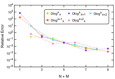
Figure 1: Relative error of the first predicted coefficient $\widehat{r}_{n}$ of $\Pi^{\prime\prime}(s)$ in the large-$\beta_{0}$ limit obtained from D-log Padé approximants applied to the Borel transform of $\Pi^{\prime\prime}(s)$. Results for ${\rm Dlog}^{M}_{N}$ shown as a function of $N+M$.

Fig. 1 shows the relative error of the first coefficient predicted by D-log Padé approximants belonging to different sequences and illustrates the convergence of the procedure. One can see that the relative errors decrease when the order of the D-log is raised. In the few cases where the error increases for higher-order approximants this can be understood in terms of the appearance of poles very far from the origin or defects (as discussed in Sec. 2) which effectively reduce the order of the approximant.

Since our goal is to apply the procedure to QCD, it is important to focus on the D-log Padés built from the first four coefficients of the series, such as the approximant of Eq. (23), which predict the coefficient of $\mathcal{O}\left(\alpha_{s}^{5}\right)$. In Fig. 1, we see that for $N+M=2$ the $\mathrm{Dlog}_{2}^{0}$ has a relative error approximately two orders of magnitude larger than $\mathrm{Dlog}_{0}^{2}$ and $\mathrm{Dlog}_{1}^{1}$. The reason for the anomalous behavior can be traced to the standard Padé $\bar{P}_{2}^{0}$ used to build the $\mathrm{Dlog}^{0}_{2}$ (see Eqs. 4 and 5). The approximant $\bar{P}_{2}^{0}$ has a pair of complex poles at $u=0.1230\pm 0.2517i$, not too far from the origin. As we discussed in Sec. 2, the complex poles can appear when the function to be approximated is meromorphic but not Stieltjes, however the Padé approximation to the function by definition breaks down close to these poles. Since we are interested in the behavior around the origin, the poles are not sufficiently far and, thus, the estimates of $\mathrm{Dlog}_{2}^{0}$ can be disconsidered since $\bar{P}_{2}^{0}$ is not a reliable approximation for the function $F(z)$ defined in Eq. 4 in the range up to the first renormalon poles.

Finally, estimates of the Borel sum obtained from the D-log Padés are very close to the true value and get better with larger $k$. Furthermore, we observe that when the order of the D-log Padé is increased, the sign-alternating behavior and the dominant pole $u=-1$ are well replicated, although for the latter often with a multiplicity that is not so close to the exact value. The quality of the results obtained from the D-log approximants in large-$\beta_{0}$ can be understood from the fact that the procedure reduces the double poles of the Borel transform to simple poles. This type of singularity softening also happens when the D-logs are applied to functions with branch cuts, which make their use appealing in full QCD.

4.2 Independent coefficients $d_{n,1}$ and partial conclusions

As we discussed in Sec. 3, the only independent coefficients of the scalar correlator are the $d_{n,1}$ of Eq. 9. It is, of course, possible to determine them from the coefficients of the second derivative of $\Pi(s)$. The relation between $d_{n,1}$ and $\widehat{r}_{n}$, the coefficients of $\Pi^{\prime\prime}(s)$ written in terms of the RGI quark mass, reads

$$d_{n,1}=\widehat{r}_{n}-\dfrac{2}{\beta_{1}}\,\gamma_{m}^{(n+1)}+\dfrac{(n-1)}{2}\,\beta_{1}d_{n-1,1}.$$ (24)

In Tab. 1 we show the coefficients $d_{n,1}$ obtained from the D-log Padé approximants that predict the coefficient of $\mathcal{O}(\alpha_{s}^{5})$. (The results from $\mathrm{Dlog}_{2}^{0}$ are not shown for the reasons already discussed.)

The predictions for the coefficients $d_{n,1}$ are in general very good. It should also be observed that the spread in their values, which is a measure of the associated error, is smaller than in the coefficients $\widehat{r}_{n}$. This occurs because the coefficients $d_{n,1}$, besides depending on the predicted $\widehat{r}_{n}$, also depend on the previous $d_{n-1,1}$ coefficients, on the $\gamma_{m}$-function coefficients, and $\beta_{1}$. The $\gamma_{m}$-function coefficients are exactly known to all orders in the large-$\beta_{0}$ limit while the coefficients $d_{n-1,1}$ are exactly known for all coefficients used as input in the construction of the approximants. Hence, the dispersion in the values of $d_{5,1}$, for example, arises solely from $\widehat{r}_{n}$, which represents just a fraction of $d_{n,1}$.

Table 1: Coefficients $d_{n,1}$ in the ${\overline{\rm MS}}$ scheme from D-log Padés built to the Borel transform of $\Pi^{\prime\prime}(s)$ together with their exact values in the large-$\beta_{0}$ limit highlighted in blue.

	$d_{5,1}$	$d_{6,1}$	$d_{7,1}$	$d_{8,1}$
Large-$\beta_{0}$ (exact)	6798	56 756	816 323	$8.86\times 10^{6}$
$\mathrm{Dlog}_{0}^{2}$	5722	49 141	573 274	$7.31\times 10^{6}$
$\mathrm{Dlog}_{1}^{1}$	6412	54 721	731 481	$8.48\times 10^{6}$

The explorations of this section exemplify the use of the D-log approximants in a realistic case. The construction of standard Padé approximants can, of course, also be explored in the large-$\beta_{0}$ limit, and they also display convergence, although somewhat slower than in the case of the D-log Padés to $\Pi^{\prime\prime}(s)$. An important point is that we were able to identify the reason behind the bad predictions of some pathological approximants, that must be discarded. This is standard procedure; PAs must always be applied judiciously and critically [22, 15]. Our explorations in large-$\beta_{0}$ favour approximants built to the Borel transform of the physical quantities that derive from the scalar correlator, namely $\operatorname{Im}\Pi(s)$ and $\Pi^{\prime\prime}(s)$, and in particular the use of the D-log Padé approximants to $\Pi^{\prime\prime}(s)$ which proved to be superior than other alternatives.

In general, however, we observe that the results for the scalar correlator are less good than the results obtained with the same procedure applied to the massless QCD Adler function [15]. Approximants that predict the coefficient of order four were not particularly good in the scalar case; it is essential to have four coefficients at least to make meaningful predictions. The reason for that is linked to more complicated structure of the Borel transforms in the case of the scalar correlator, which reflect the non-vanishing anomalous dimension.

Other methods to accelerate convergence, such as continuous scheme changes, departing from the ${\overline{\rm MS}}$ value $C=0$, can be exploited in the large-$\beta_{0}$ limit [25, 15, 30]. But since the application of these methods is not so straightforward in full QCD, they become somewhat academical. We will not pursue their investigation here and refer to Ref. [15] for analogous explorations in a similar context.

5 Results in QCD

In the previous section, we discussed an application of our method to results in the large-$\beta_{0}$ limit. The D-log Padé approximants to the Borel transform of the second derivative of $\Pi(s)$ proved to be most efficient with the number of coefficients we have in QCD, for the reasons already discussed. In QCD, the renormalons of the perturbative series are at the same position of the renormalons in the large-$\beta_{0}$ limit, but they become branch cuts instead of isolated poles [19, 20]. Even though there are no theorems that state the convergence of the Padé approximants to series with branch cuts in general, in many practical applications there are indications that this convergence happens and the mechanism for this apparent convergence is understood [28]. The use of D-log Padé approximants remains appealing, since these approximants are designed to deal with functions that have branch cuts.

In this section we will obtain the higher-order QCD corrections to the decay rate of the Higgs into bottom quarks. We analyze the Padé and the D-log Padé approximants to the Borel transform of the reduced imaginary part and of the second derivative of the scalar correlator in QCD.

5.1 Approximants to Im$\Pi(s)$ in QCD

We apply now the Padé-Borel method to the Borel transform of the perturbative series of the reduced imaginary part of $\Pi(s)$ as a function of the scale-dependent quark mass. The perturbative coefficients of this series in QCD are given in Eq. 12 and the Borel transform is obtained with Eq. (16). The branch-cut singularities of the Borel transform are expected to be at $u=-1,-2,\dots$ and $u=2,3,4,\dots$.

The application of standard PAs to this Borel transform leads to very discrepant results, with different signs and orders of magnitude for the coefficients of order 5 and 6. An exploration in the large-$\beta_{0}$ limit supports this finding, and the PAs are also not ideal in that limit. The difficulties of the PAs can be understood from the general structure of the Borel transform of Eq. (18). First, in QCD the prefactor $\sin(\pi u)$ is unknown, but in similar applications to the Adler function it has been shown that the same factor is present in QCD [31, 32] provided a change to the so-called $C$ scheme is used [30] — we expect the same to happen here. However, the poles turn into branch points which means that we should not expect exact cancellations from this prefactor. This means that applications of our procedure to $\operatorname{Im}\Pi(s)$ are not favoured, since the branch cuts remain branch cuts. The instabilities we find and the general structure of the Borel transform inferred from the large-$\beta_{0}$ results lead us to conclude that PAs are not ideal in this case and these results should be discarded.

We turn now to D-log Padé approximants, which are arguably superior in this case, since we are dealing with a function that has superimposed branch cuts. The approximants that forecast the last known coefficient, $c_{4}$, are $\mathrm{Dlog}_{1}^{0}$ and $\mathrm{Dlog}_{0}^{1}$. The prediction of the first one is not particularly good, the relative error is 88%, but the estimate of the second one is quite close to the original value, it has an error of mere 9%. The results for the D-log Padés that predict the first unknown coefficient of $\operatorname{Im}\Pi(s)$, $c_{5}$, are in the second and third rows of Tab. 2, except for $\mathrm{Dlog}_{2}^{0}$ because the Padé $\bar{P}_{2}^{0}$ used to build this approximant has a pair of complex poles close to the origin. We can notice that the coefficients predicted in Tab. 2 are similar and very stable. The results from these two D-log approximants are the most reliable in this case and will be part of our final results. Finally, we observe that the predicted coefficients in the second and third lines of Tab. 2 do not show a systematic sign alternation, which may indicate that in QCD the dominance of the leading UV singularity is postponed to higher orders (as observed in other contexts [15, 33]).

Table 2: Perturbative coefficients of $\operatorname{Im}\Pi(s)$, $c_{n}$, for $N_{f}=5$ predicted by PAs and D-log PAs in QCD. In “method” we indicate if the results were obtained from the Borel transforms or from the $\alpha_{s}$ expansion.

	method	$c_{5}$	$c_{6}$	$c_{7}$	$c_{8}$	$c_{9}$
$\mathrm{Dlog}_{1}^{1}$	$B[\operatorname{Im}\Pi(s)]$	$-5598$	36 053	611 562	$-1.84\times 10^{6}$	$-7.95\times 10^{7}$
$\mathrm{Dlog}_{0}^{2}$	$B[\operatorname{Im}\Pi(s)]$	$-5526$	37 812	616 726	$-2.21\times 10^{6}$	$-8.37\times 10^{7}$
$P_{1}^{2}$	$B[\Pi^{\prime\prime}(s)]$	$-8142$	$-26\,272$	171 244	$2.52\times 10^{6}$	$1.09\times 10^{7}$
$P_{2}^{1}$	$B[\Pi^{\prime\prime}(s)]$	$-8198$	$-27\,773$	153 734	$2.43\times 10^{6}$	$1.11\times 10^{7}$
$\mathrm{Dlog}_{2}^{0}$	$B[\Pi^{\prime\prime}(s)]$	$-8149$	$-26\,626$	164 374	$2.46\times 10^{6}$	$1.06\times 10^{7}$
$\mathrm{Dlog}_{0}^{2}$	$B[\Pi^{\prime\prime}(s)]$	$-8033$	$-24\,558$	163 186	$2.09\times 10^{6}$	$6.98\times 10^{6}$
$P_{1}^{3}$	$\Pi^{\prime\prime}(\alpha_{s})$	$-8341$	$-31\,410$	118 321	$2.41\times 10^{6}$	$1.45\times 10^{7}$
$P_{3}^{1}$	$\Pi^{\prime\prime}(\alpha_{s})$	$-8340$	$-31\,480$	116 501	$2.41\times 10^{6}$	$1.47\times 10^{7}$

5.2 Results for $\Pi^{\prime\prime}(s)$ in QCD

We turn now to the approximants built to the Borel transform of $\Pi^{\prime\prime}(s)$ which were the basis for the optimal strategy in large-$\beta_{0}$, described in Sec. 4. We expect the D-log Padés to be efficient here as well since they can deal with the branch cuts more easily. An advantage of working with the Borel transform of $\Pi^{\prime\prime}(s)$ is that the Padés do not have to reproduce the QCD counterpart of the $\sin(\pi u)$ which appears in the Borel transform of $\operatorname{Im}\Pi(s)$.

We built all PAs and D-log Padé approximants that post-dict the fourth- or predict the fifth-order coefficient. The PAs $P_{2}^{0}$ and $P_{3}^{0}$ have a pair of complex poles relatively close to the origin and are discarded as per the explanations of Secs. 2 and 4. Also, we do not consider the results of $\mathrm{Dlog}_{1}^{1}$ because the Padé $\bar{P}_{1}^{1}$ used to build this D-log has an almost defect: a pole at $u=-0.1998$ and a close-by zero at $u=-0.2170$, which, as we saw in Sec. 4, effectively reduces the order of the PA and produces untrustworthy estimates.

The post-diction of $P_{1}^{1}$ for the fourth-order coefficient of $\Pi^{\prime\prime}(s)$ is accurate: the error is about 20%. The estimates of $r_{4}$ from $\mathrm{Dlog}_{0}^{1}$ and $\mathrm{Dlog}_{1}^{0}$ are also close to the exact value with an error of only $\sim 30$%. The good quality of these results is certainly reassuring but we observe that for higher orders the predictions of these approximants can differ significantly — a fact that is in line with our conclusion that with less than four input coefficients the quality of the predictions from the approximants deteriorates quickly.

The results for the approximants that predict the fifth order (and higher) coefficients are shown from lines three to six of Tab. 2. The results from the PAs and D-log Padé approximants that pass all reliability tests are all stable and are mutually consistent. These results will also enter our final estimate for the higher order coefficients.

Regarding the renormalons, we observe that all predicted coefficients of $\Pi^{\prime\prime}(s)$ up to order 9 are positive, with no sign of the dominance of the UV renormalon. Furthermore, all the PAs that use all known coefficients have singularities on the positive real axis. $\mathrm{Dlog}_{2}^{0}$ predicts a cut on the positive real axis at $u=1.642$ with multiplicity $\gamma=1.2799$. All of this indicates that in QCD $\Pi^{\prime\prime}(s)$ is more dominated by the IR renormalons at intermediate orders.

5.2.1 Padés to the Series in $\alpha_{s}$ in QCD

A possible way to corroborate the results we found previously is to perform PAs directly to the series in powers of $a_{s}$. Even though these approximants are less interesting since we lose part of the connection with renormalons and experience shows that for divergent series it is advantageous to work with the Padé-Borel method, they provide an additional check of the robustness of the results. We have built PAs to the series expansion in powers of $a_{s}$ of $\operatorname{Im}\Pi(s)$ and $\Pi^{\prime\prime}(s)$. The PAs to $\operatorname{Im}\Pi(s)$ are problematic because they have Froissart doublets or complex poles dangerously close to the origin. In addition, one can notice from Eq. 14 that the perturbative series of the second derivative in QCD is very regular until fourth order, i.e., there is no change of sign and the known coefficients are stable (the divergent behavior is not evident up to fourth-order). Because of these two facts, we report the results of PAs built to the expansion of $\Pi^{\prime\prime}(s)$ in powers of $a_{s}$.

Regarding the post-diction of the last known coefficient, the results for $r_{4}$ from the Padés $P_{1}^{2}$ and $P_{2}^{1}$ are in good agreement with the exact value, with an error of approximately 20%. Results from the PAs that predict the first unknown coefficient are shown in the last two rows of Tab. 2, where we can see that they are stable. (The results for $P_{2}^{2}$ are not on the table because it has a defect.) Analyzing the predicted coefficients of $\Pi^{\prime\prime}(s)$ from these PAs, we can notice that all the coefficients are again positive, which corroborates the dominance of the IR renormalons at lower and intermediate orders. However, the central values of the coefficients up to seventh order given in the last two rows of Tab. 2 are lower than the ones obtained before. Even though there is reason to believe the results from the Padé-Borel approximants to be superior we will also use these latter results in our final values to remain fully conservative.

5.3 Final results and uncertainties in $H\to b\bar{b}$

In this section we will obtain our final values for the higher-order coefficients of the perturbative expansion of $\operatorname{Im}\Pi(s)$. The final results will be based on the approximants of Tab. 2. We will not use approximants that post-dict the $\mathcal{O}(\alpha_{s}^{3})$ coefficient since in the large-$\beta_{0}$ limit we found that with only three coefficients the rational approximants lack information to correctly predict the series beyond the fourth or fifth order. Approximants based on $\operatorname{Im}\Pi(s)$ give results that differ significantly from the other approximants, especially for orders $\alpha_{s}^{6}$ and higher. As discussed before, the general structure of the Borel transform of $\operatorname{{\rm Im}}\Pi(s)$ suggests that it is not optimal to work with this quantity. However, to remain maximally conservative, and bearing in mind that our primary interest is on the series for $\operatorname{{\rm Im}}\Pi(s)$, we keep these results in our final analysis, which lead to larger (but very conservative) errors.

We start by computing the independent coefficients of the perturbative expansion of $\Pi(s)$, $d_{n,1}$, as we did in Sec. 4.2. The relation between the coefficients of $\Pi(s)$, $\operatorname{Im}\Pi(s)$, and $\Pi^{\prime\prime}(s)$ can be easily found from the expressions of Sec. 3 (additional useful formulas can be found in Ref. [25]). In order to extract $d_{n,1}$ with $5\leq n\leq 8$ from our results given in Tab.  2 we need, in principle, the coefficients of the $\beta$ and $\gamma_{m}$ functions up to $\beta_{7}$ and $\gamma_{m}^{(8)}$, respectively. Since we know exactly only the coefficients up to five loops, we will consider the unknown higher-order terms of the $\beta$ and $\gamma_{m}$ functions equal to zero, i.e., $\beta_{6}=\beta_{7}=0$ and $\gamma_{m}^{(6)}=\gamma_{m}^{(7)}=\gamma_{m}^{(8)}=0$. This is a reasonable approximation since there is no sign of a possible divergence for these expansions [34, 35, 36], in agreement with the (unproven) conjecture that the ${\overline{\rm MS}}$ scheme is a regular scheme, i.e., a scheme where the $\beta$ and $\gamma_{m}$ functions are convergent series or at least do not diverge as fast as a factorial[19]. As a check of the reliability of this approximation, we also computed the coefficients $d_{5,1}$ zeroing the last known coefficients, $\beta_{5}$ and $\gamma_{m}^{(5)}$, and compared with the results found using the known values of $\gamma_{m}^{(5)}$ and $\beta_{5}$. The difference did not exceed 0.21%, which confirms that the truncation of the $\beta$ and $\gamma_{m}$ function at the fifth term is, very likely, a very good approximation for our purposes. This assumption will be used in the rest of this work.

Table 3: Final values for the perturbative coefficients of $\Pi(s)$, $d_{n,1}$, from the Padé and D-log Padé approximants to the perturbative expansions of $\operatorname{Im}\Pi(s)$ and $\Pi^{\prime\prime}(s)$ in QCD (${\overline{\rm MS}}$ scheme, $N_{f}=5$).

$d_{5,1}$	$d_{6,1}$	$d_{7,1}$	$d_{8,1}$
$(4.22\pm 0.14)\times 10^{4}$	$(5.79\pm 0.35)\times 10^{5}$	$(8.87\pm 0.61)\times 10^{6}$	$(1.51\pm 0.11)\times 10^{8}$

The coefficients $d_{n,1}$ were calculated from the estimated values of $c_{n}$ and $r_{n}$, the coefficients of the imaginary part and the second derivative of the scalar correlator respectively, given in Tab. 2; the final results for $d_{n,1}$ are in Tab. 3. The central values are calculated as the average between the largest and the smallest estimated coefficients. We assign an error to each coefficient that represents the maximum spread found between results from two approximants divided by two (a prescription that will be used through this work, and that is corroborated by explorations in large-$\beta_{0}$).

With the same prescription we can also calculate the higher-order coefficients $c_{n}$ of the imaginary part of $\Pi(s)$, directly related to $\Gamma(H\to b\bar{b})$. Our final result for the six-loop coefficient, $c_{5}$, the first unknown in QCD, is then

$$c_{5}=-6900\pm 1400,$$ (25)

where the uncertainty is obtained from the spread in values from the different approximants, as explained above. Results up to $c_{8}$ are shown in Tab. 4. An important, if obvious, remark is that our errors should not be interpreted in a statistical sense. Rather, they give an interval where we expect the true value of the coefficients to lie. Our final estimate for the intrinsic error in $c_{5}$, of about $20\%$, has a small impact in the sum of the perturbative series due to the suppression by $\alpha_{s}^{5}$— as we will show in detail below. For the coefficients of sixth-order or higher, the errors associated are greater than 100%, but they again do not lead to very large errors in the perturbative expansion. We remark that the estimated coefficients $c_{n}$ are not systematically sign-alternating, which suggests a competition between IR and UV renormalons at intermediate orders in QCD, in contrast with the typical situation in large-$\beta_{0}$, as observed in related computations [15, 33].

Let us compare our result for $c_{5}$ with other estimates in the literature. This comparison is not completely straightforward since other estimates do not have associated errors. The first method, applied by Bakulev, Mikhailov and Stefanis [37], models the coefficients of the series with two parameters, which are determined through the known coefficients. With their estimated value for $d_{5,1}$ we can calculate their central value for $c_{5}$, which is $-4052$; this result is not compatible with ours given the size and nature of our uncertainties in Eq. (25). In Ref. [37] the coefficient $d_{5,1}$ is also calculated using the strategy employed by Kataev and Starshenko [38], the Principle of Minimal Sensitivity (PMS), and the value obtained for $c_{5}$ is $-6886$ which is fully compatible with our prediction.

It is also interesting to extract a final estimate for the Borel integral of the reduced $\operatorname{Im}\Pi(s)$, the function $F(a_{s})$ of Eq. (12), which corresponds to an estimate of the all-order true value of the series. In order to obtain this value, we calculated the perturbative series of $\operatorname{Im}\Pi(s)$ predicted by each approximant of Tab. 2. The ambiguity of the Borel integral, associated with non-perturbative corrections and quantified by its imaginary part, is tiny in the application to Higgs decays, where the typical scale is $m_{H}$. We have checked that for all practical purposes it can be neglected. Therefore, in this case, since the integrand is suppressed exponentially, the representative value of the integral can be obtained by simply integrating the Taylor expansion of the Borel transformed $\operatorname{Im}\Pi(s)$. We have checked the reliability of this procedure in cases where an analytical integration of the PAs was possible, and found that it leads to stable and correct results. For $\alpha_{s}(m_{H})=0.1125\pm 0.0009$, the final value obtained for the reduced $\operatorname{Im}\Pi(s)$ is

$$F=0.2405\pm(0.0022)_{\alpha_{s}}\pm(0.0002)_{\mathrm{PA}},$$ (26)

where the first error is due to the uncertainty in the strong coupling, which largely dominates, and the second is due to the spread in the results from different approximants. Our result is in good agreement with the one determined through the Principle of Maximum Conformality (PMC) [39, 40], which yields $0.2405\pm 0.0001$, where the uncertainty is intrinsic to the method.

Table 4: Final values for the QCD perturbative coefficients $c_{n}$ of $\operatorname{Im}\Pi(s)$ (${\overline{\rm MS}}$ scheme, $N_{f}=5$).

$c_{5}$	$c_{6}$	$c_{7}$	$c_{8}$
$-6900\pm 1400$	$(0.3\pm 3.5)\times 10^{4}$	$(3.7\pm 2.5)\times 10^{5}$	$(0.2\pm 2.4)\times 10^{6}$

We apply now our final results to an analysis of the uncertainties in the SM calculation of $\Gamma(H\rightarrow b\bar{b})$. Let us start from a discussion of the residual renormalization scale dependence order by order. As customary in the literature [41], we study the ratio

$$\frac{\Gamma(H\to b\bar{b})(\mu)}{\Gamma(H\to b\bar{b})_{\rm LO}(m_{H})}=\frac{m_{b}^{2}(\mu)}{m_{b}^{2}(m_{H})}\sum_{n=0}a_{s}^{n}(\mu)\sum_{j=0}^{n}c_{n,j}\ln^{j}\left(m_{H}^{2}/\mu^{2}\right),$$ (27)

where the dependent coefficients $c_{n,j}$ can be obtained using the RGE and $c_{n,0}\equiv c_{n}$. We calculate this quantity as a function of the renormalization scale $\mu$, which was varied in the range $m_{H}/2\leq\mu\leq 2m_{H}$, and the final result up to N5LO, computed using our prediction for the $c_{5}$ value of Eq. (25), is in Fig. 2. At N4LO the renormalization-scale is already mild and it is further reduced at N5LO calculated from our value of $c_{5}$, as expected.

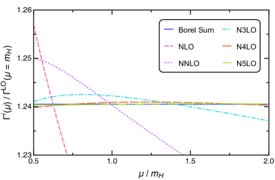
Figure 2: Renormalization scale dependence of the normalized decay width given in Eq. (27).

Numerically, the perturbative evaluation of $\Gamma(H\to b\bar{b})(\mu)$ with $\mu=m_{H}$ up to our predicted contribution at N5LO, order by order, gives

$$\frac{\Gamma(H\to b\bar{b})(m_{H})}{\Gamma(H\to b\bar{b})_{\rm LO}(m_{H})}=1+0.20295+0.03738+0.00192-0.00136-\boxed{0.00041(8)_{\rm PAs}},$$ (28)

where the boxed term is the predicted N5LO result with the uncertainty stemming from the approximants. We display this series, order by order in perturbation theory, for three different choices of the renormalization scale $\mu$, in Figs. 3 and 3. The error bars give the error from the series coefficients in Tab. 4. The horizontal bands show the predicted value for the all order result, Eq. (26), with the uncertainties from $\alpha_{s}$ and from the PAs. We see that at N4LO, due to the reduced renormalization scale dependence, the final uncertainty starts to be dominated by $\alpha_{s}$. At N5LO and beyond, the series behaves essentially as if it had already converged with a tiny $\mu$-dependence and an excellent agreement with our predicted all-order result. Our results for the 6-loop coefficient and for the estimated true value of the series confirm that the QCD perturbative series is under excellent control for this observable although the precision in $\alpha_{s}$ (and $m_{b}$) must be increased in order to make the most of the perturbative calculation.

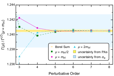
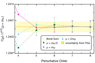
Figure 3: Perturbative expansion of the normalized decay rate Eq. (27) in QCD at three different renormalization scales using the coefficients of Tab. 4 for the coefficients $c_{n\geq 5}$ and the integral given in Eq. 26. The uncertainty of the Borel integral is due to (a) the strong coupling uncertainty (light-blue band) and (b) the different Padé predictions (light-yellow band). The uncertainty from $m_{b}$ essentially cancels in Eq. (27). The error bars of the points in (b) are due to the errors of the predicted coefficients. The $\alpha_{s}$ uncertainty is omitted in (b) since it would be too large for the scale of the figure.

At N5LO, we find for the decay width of the Higgs into bottom quarks

$$\Gamma(H\rightarrow b\bar{b})=2.3806 (^{+0.041}_{-0.027})_{m_{b}}\pm(0.0042)_{\alpha_{s}}$$

$$\pm(0.0032)_{m_{H}}\pm(0.0002)_{\mu}\pm(0.0003)_{\mathrm{PAs}}\,\,\mathrm{MeV},$$ (29)

where the uncertainty marked with $\mu$ refers to renormalization scale variation. In this result we have used $m_{b}(m_{b})=4.18^{+0.03}_{-0.02}$ GeV, $m_{H}=125.25\pm 0.17$ GeV, $\alpha_{s}(m_{Z})=0.1179\pm 0.0010$ [46], together with our result $c_{5}=-6900\pm 1400$. The use of the all-order estimate of Eq. (26) would lead to an almost identical result, since at N5LO the series is reaching its true value. The uncertainty from renormalization scale variation was calculated as half of the maximum dispersion of the decay rate found when the scale was varied in the interval $m_{H}/2\leq\mu\leq 2\,m_{H}$. The inclusion of our N5LO result reduces the error due to scale variation by a factor of $4.3$ (it would be $\pm 0.001$ at N4LO). The largest contributions to the error arise from the QCD parameters, $m_{b}$ and $\alpha_{s}$, as well as the Higgs mass. (The size of our uncertainties from these parameters agrees with those of [3] when the same input values are used.) This is an example of a process where perturbative QCD is under excellent control, as could be inferred from the perturbative uncertainties associated with the result at $\mathcal{O}(\alpha_{s}^{4})$, and the intrinsic uncertainty from the truncation of the series is tamed for the present purposes. With our estimated N5LO result, and conservatively adding in quadrature the errors from scale variation and from the PAs, the truncation uncertainty does not exceed $0.02\%$.

6 Conclusions

We have applied the Padé-Borel method to study missing higher orders (MHOs) in the massless scalar-current quark correlator. The method we use was first applied to the Adler function in Ref. [15]. We make use of the knowledge available in the large-$\beta_{0}$ limit to guide our study in QCD. This is important given that the available information about the series expansion in QCD is not abundant: only the first four non-trivial terms are known. In particular, the results in large-$\beta_{0}$ are used in order to select the variants of the approximants that lead to faster convergence with only four coefficients used as input. They are also instrumental for the QCD analysis, since the general structure of the Borel transforms in QCD can be inferred from the large-$\beta_{0}$ results.

Our main result is the prediction for the MHOs in $\operatorname{Im}\Pi(s)$, which is directly connected to $\Gamma(H\to b\bar{b})$. We forecast the six-loop result to be $c_{5}=-6900\pm 1400$. We have shown that with this result the series is essentially immune to renormalization scale variations and the perturbative uncertainty becomes tiny: its does not exceed $0.02\%$. Our predictions for the MHOs and for the true value of the series indicate that the perturbative expansion is very well behaved even at higher orders and approaches smoothly the true value as predicted by the rational approximants, as can be seen in Fig. 3. Although this could be inferred from the analysis of the series truncated at $\mathcal{O}(\alpha_{s}^{4})$, it is reassuring to see it confirmed after the inclusion of our estimates for higher orders. Additionally, the coefficients of Tab. 2 do not show a systematic sign alternation, which implies that the dominance of the UV renormalon is still not established.

As far as the SM uncertainty in $\Gamma(H\to b\bar{b})$ is concerned, higher-loop calculations for the contributions discussed here, namely those associated with the massless scalar correlator, are probably not warranted. For the purposes of matching the experimental uncertainty that should be achieved in the FCC-ee [2, 3], for example, the result at 5 loops together with our estimate of the MHOs should suffice. The SM precision will be driven by the progress that can be made in the determination of $m_{b}$ and, to a lesser extend, of $\alpha_{s}$.

Appendix A QCD $\beta$ and $\gamma_{m}$ functions and scale invariant quark mass

Our definitions for the $\beta$ and $\gamma_{m}$ functions are

$$\beta(a_{s})\equiv-\mu\,\dfrac{\mathrm{d}a_{s}}{\mathrm{d}\mu}=\beta_{1}a_{s}^{2}+\beta_{2}a_{s}^{3}+\beta_{3}a_{s}^{4}+\cdots,$$ (30)

$$\gamma_{m}(a_{s})\equiv-\frac{\mu}{m_{q}}\,\dfrac{\mathrm{d}m_{q}}{\mathrm{d}\mu}=\gamma_{m}^{(1)}a_{s}+\gamma_{m}^{(2)}a_{s}^{2}+\gamma_{m}^{(3)}a_{s}^{3}+\cdots,$$ (31)

with $a_{s}\equiv\alpha_{s}/\pi$. For definiteness, we give the one-loop coefficients of these functions:

$$\beta_{1}=\frac{11}{2}-\frac{N_{f}}{3},\qquad{\rm and}\qquad\gamma_{m}^{(1)}=2.$$ (32)

With these definitions, the RGI quark mass can be written as

$$m_{q}(\mu)\equiv\widehat{m}_{q}\,[\alpha_{s}(\mu)]^{\gamma_{m}^{(1)}/\beta_{1}}\,\mathrm{exp}\left\{\int\displaylimits_{0}^{a_{s}(\mu)}\mathrm{d}a\left[\dfrac{\gamma_{m}(a)}{\beta(a)}-\dfrac{\gamma_{m}^{(1)}}{\beta_{1}a}\right]\right\}.$$ (33)

References

- [1] FCC collaboration, FCC Physics Opportunities: Future Circular Collider Conceptual Design Report Volume 1, Eur. Phys. J. C 79 (2019) 474.
- [2] S. Heinemeyer, S. Jadach and J. Reuter, Theory requirements for SM Higgs and EW precision physics at the FCC-ee, Eur. Phys. J. Plus 136 (2021) 911 [2106.11802].
- [3] A. Freitas et al., Theoretical uncertainties for electroweak and Higgs-boson precision measurements at FCC-ee, 1906.05379.
- [4] ATLAS collaboration, Observation of decays and production with the ATLAS detector, Phys. Lett. B 786 (2018) 59 [1808.08238].
- [5] CMS collaboration, Observation of Higgs boson decay to bottom quarks, Phys. Rev. Lett. 121 (2018) 121801 [1808.08242].
- [6] E. Braaten and J. P. Leveille, Higgs Boson Decay and the Running Mass, Phys. Rev. D 22 (1980) 715.
- [7] N. Sakai, Perturbative QCD Corrections to the Hadronic Decay Width of the Higgs Boson, Phys. Rev. D 22 (1980) 2220.
- [8] K. G. Chetyrkin, R. Harlander and M. Steinhauser, Singlet polarization functions at O (alpha-s**2), Phys. Rev. D 58 (1998) 014012 [hep-ph/9801432].
- [9] P. A. Baikov, K. G. Chetyrkin and J. H. Kuhn, Scalar correlator at , Higgs decay into b-quarks and bounds on the light quark masses, Phys. Rev. Lett. 96 (2006) 012003 [hep-ph/0511063].
- [10] F. Herzog, B. Ruijl, T. Ueda, J. A. M. Vermaseren and A. Vogt, On Higgs decays to hadrons and the R-ratio at N4LO, JHEP 08 (2017) 113 [1707.01044].
- [11] J. Davies, M. Steinhauser and D. Wellmann, Completing the hadronic Higgs boson decay at order , Nucl. Phys. B 920 (2017) 20 [1703.02988].
- [12] M. Spira, Higgs Boson Production and Decay at Hadron Colliders, Prog. Part. Nucl. Phys. 95 (2017) 98 [1612.07651].
- [13] G. A. Baker, Essentials of Padé approximants. Academic Press, New York, 1, 1975.
- [14] G. A. Baker and P. Graves-Morris, Padé approximants: Encyclopedia of mathematics and it’s applications. Cambridge University Press, Cambridge, 2 ed., 1996, 10.1017/CBO9780511530074.
- [15] D. Boito, P. Masjuan and F. Oliani, Higher-order QCD corrections to hadronic decays from Padé approximants, JHEP 08 (2018) 075 [1807.01567].
- [16] P. A. Baikov, K. G. Chetyrkin and J. H. Kuhn, Order QCD Corrections to and Decays, Phys. Rev. Lett. 101 (2008) 012002 [0801.1821].
- [17] M. Beneke and V. M. Braun, Naive non-abelianization and resummation of fermion bubble chains, Phys. Lett. B348 (1995) 513 [hep-ph/9411229].
- [18] D. J. Broadhurst and A. G. Grozin, Matching QCD and HQET heavy - light currents at two loops and beyond, Phys. Rev. D 52 (1995) 4082 [hep-ph/9410240].
- [19] M. Beneke, Renormalons, Phys. Rept. 317 (1999) 1 [hep-ph/9807443].
- [20] M. Jamin, Higher-order behaviour of two-point current correlators, 2106.01614.
- [21] P. Masjuan Queralt, Rational Approximations in Quantum Chromodynamics, other thesis, 5, 2010.
- [22] P. Masjuan and S. Peris, A Rational approach to resonance saturation in large- QCD, JHEP 05 (2007) 040 [0704.1247].
- [23] P. Masjuan and S. Peris, A Rational approximation to VV-AA and its O() low-energy constant, Phys. Lett. B 663 (2008) 61 [0801.3558].
- [24] P. Masjuan and S. Peris, Pade Theory applied to the vacuum polarization of a heavy quark, Phys. Lett. B 686 (2010) 307 [0903.0294].
- [25] M. Jamin and R. Miravitllas, Scalar correlator, Higgs decay into quarks, and scheme variations of the QCD coupling, JHEP 10 (2016) 059 [1606.06166].
- [26] K. G. Chetyrkin, Correlator of the quark scalar currents and at in pQCD, Phys. Lett. B 390 (1997) 309 [hep-ph/9608318].
- [27] M. A. Samuel, J. R. Ellis and M. Karliner, Comparison of the Pade approximation method to perturbative QCD calculations, Phys. Rev. Lett. 74 (1995) 4380 [hep-ph/9503411].
- [28] O. Costin and G. V. Dunne, Conformal and Uniformizing Maps in Borel Analysis, 2108.01145.
- [29] D. J. Broadhurst, A. L. Kataev and C. J. Maxwell, Renormalons and multiloop estimates in scalar correlators: Higgs decay and quark mass sum rules, Nucl. Phys. B 592 (2001) 247 [hep-ph/0007152].
- [30] D. Boito, M. Jamin and R. Miravitllas, Scheme variations of the QCD coupling and tau decays, Nucl. Part. Phys. Proc. 287-288 (2017) 77 [1612.05558].
- [31] L. S. Brown, L. G. Yaffe and C.-X. Zhai, Large order perturbation theory for the electromagnetic current current correlation function, Phys. Rev. D46 (1992) 4712 [hep-ph/9205213].
- [32] D. Boito and F. Oliani, Renormalons in integrated spectral function moments and extractions, Phys. Rev. D 101 (2020) 074003 [2002.12419].
- [33] D. Boito, V. Mateu and M. V. Rodrigues, Small-momentum expansion of heavy-quark correlators in the large-0 limit and s extractions, JHEP 08 (2021) 027 [2106.05660].
- [34] P. A. Baikov, K. G. Chetyrkin and J. H. Kühn, Five-Loop Running of the QCD coupling constant, Phys. Rev. Lett. 118 (2017) 082002 [1606.08659].
- [35] P. A. Baikov, K. G. Chetyrkin and J. H. Kühn, Quark Mass and Field Anomalous Dimensions to , JHEP 10 (2014) 076 [1402.6611].
- [36] F. Herzog, B. Ruijl, T. Ueda, J. A. M. Vermaseren and A. Vogt, The five-loop beta function of Yang-Mills theory with fermions, JHEP 02 (2017) 090 [1701.01404].
- [37] A. P. Bakulev, S. V. Mikhailov and N. G. Stefanis, Higher-order QCD perturbation theory in different schemes: From FOPT to CIPT to FAPT, JHEP 06 (2010) 085 [1004.4125].
- [38] A. L. Kataev and V. V. Starshenko, Estimates of the higher order QCD corrections to R(s), R(tau) and deep inelastic scattering sum rules, Mod. Phys. Lett. A 10 (1995) 235 [hep-ph/9502348].
- [39] B.-L. Du, X.-G. Wu, J.-M. Shen and S. J. Brodsky, Extending the Predictive Power of Perturbative QCD, Eur. Phys. J. C 79 (2019) 182 [1807.11144].
- [40] X.-G. Wu, J.-M. Shen, B.-L. Du, X.-D. Huang, S.-Q. Wang and S. J. Brodsky, The QCD renormalization group equation and the elimination of fixed-order scheme-and-scale ambiguities using the principle of maximum conformality, Prog. Part. Nucl. Phys. 108 (2019) 103706 [1903.12177].
- [41] R. Mondini, M. Schiavi and C. Williams, N3LO predictions for the decay of the Higgs boson to bottom quarks, JHEP 06 (2019) 079 [1904.08960].
- [42] K. G. Chetyrkin, J. H. Kuhn and M. Steinhauser, RunDec: A Mathematica package for running and decoupling of the strong coupling and quark masses, Comput. Phys. Commun. 133 (2000) 43 [hep-ph/0004189].
- [43] F. Herren and M. Steinhauser, Version 3 of RunDec and CRunDec, Comput. Phys. Commun. 224 (2018) 333 [1703.03751].
- [44] N. G. Stefanis, Taming Landau singularities in QCD perturbation theory: The Analytic approach, Phys. Part. Nucl. 44 (2013) 494 [0902.4805].
- [45] S.-Q. Wang, X.-G. Wu, X.-C. Zheng, J.-M. Shen and Q.-L. Zhang, The Higgs boson inclusive decay channels and up to four-loop level, Eur. Phys. J. C 74 (2014) 2825 [1308.6364].
- [46] Particle Data Group collaboration, Review of Particle Physics, PTEP 2020 (2020) 083C01.
- [47] B. Dehnadi, A. H. Hoang and V. Mateu, Bottom and Charm Mass Determinations with a Convergence Test, JHEP 08 (2015) 155 [1504.07638].
- [48] D. Boito and V. Mateu, Precise determination of from relativistic quarkonium sum rules, JHEP 03 (2020) 094 [2001.11041].