Time Series Analysis via Network Science: Concepts and Algorithms

Abstract

There is nowadays a constant flux of data being generated and collected in all types of real world systems. These data sets are often indexed by time, space or both requiring appropriate approaches to analyze the data. In univariate settings, time series analysis is a mature and solid field. However, in multivariate contexts, time series analysis still presents many limitations. In order to address these issues, the last decade has brought approaches based on network science. These methods involve transforming an initial time series data set into one or more networks, which can be analyzed in depth to provide insight into the original time series. This review provides a comprehensive overview of existing mapping methods for transforming time series into networks for a wide audience of researchers and practitioners in machine learning, data mining and time series. Our main contribution is a structured review of existing methodologies, identifying their main characteristics and their differences. We describe the main conceptual approaches, provide authoritative references and give insight into their advantages and limitations in a unified notation and language. We first describe the case of univariate time series, which can be mapped to single layer networks, and we divide the current mappings based on the underlying concept: visibility, transition and proximity. We then proceed with multivariate time series discussing both single layer and multiple layer approaches. Although still very recent, this research area has much potential and with this survey we intend to pave the way for future research on the topic.

Keywords: univariate time series, multivariate time series, network science, mapping methods

1 Introduction

The recent developments in technology are leading to the generation and collection of huge volumes of data associated with various real world systems. These data sets typically exhibit an inherent temporal dimension that is crucial to their understanding. The analysis of a single collection of observations indexed in time in a univariate setting is a mature and solid field, usually referred to as time series analysis (Shumway and Stoffer,, 2017), which mostly involves statistical linear analysis. Given that many observed data sets exhibit non-Gaussian and non-linear characteristics, in the last decades several statistical non-Gaussian and non-linear models have been proposed in the literature (Douc et al.,, 2014). These models have often been developed tailored to model data from specific areas and under several assumptions that hinder their wide application (Wei,, 2019). In fact, in many settings both univariate (e.g. high frequency signals, non-stationarity) and high dimensional (e.g. multivariate, spatio-temporal, panels of time series) time series analysis still presents many limitations. An alternative approach to time series data analysis has been developed under the framework of dynamical systems theory. This approach, denominated nonlinear time-series analysis (Bradley and Kantz,, 2015) can be overly effective when the data model is based o deterministic dynamics in some state space.

Network science is nowadays a well established field of science that studies a wide range of systems in nature and society, by representing the existing interactions through complex network (or graph) structures (Barabási,, 2016). There exists a vast set of topological graph measurements available (Costa et al.,, 2007), a well-defined set of problems and a large track record of successful application of complex network methodologies to different fields (Vespignani,, 2018).

In the last decade, several approaches for time series analysis based on network science methodologies were proposed, leveraging the large body of research in network analysis and providing new insight and novel angles on which to understand the structure of time series (Zou et al.,, 2019). This new framework for time series analysis inevitably involves mapping the time series into networks. This survey aims precisely to provide a comprehensive overview of the existing mapping methods for this purpose. Our main contribution is to produce a general and structured review of existing mapping algorithms, highlighting their similarities and differences, the data characteristics they capture and the main references and results. We propose here a conceptual division of the methods at the level of the time series dimensionality and concomitant choice of the resulting network structure. From our point of view, this high-level conceptual division encompasses all existing methods in the literature, for both univariate and multivariate frameworks.

The proposed high-level conceptual division is depicted in the diagram of Figure 1, and corresponds to the organization of our paper. We first divide the mappings into two large groups, depending on the source data set being a univariate or a multivariate time series. The first group results in single layer networks, while multivariate series can be mapped both in single layer and in multiple layer networks (such as multiplex networks).

Figure 1: Overview of our survey. Taxonomy of algorithms for mapping time series into complex networks based on the dimensionality of time series, resulting network structure, mapping concept, and main mapping methods.

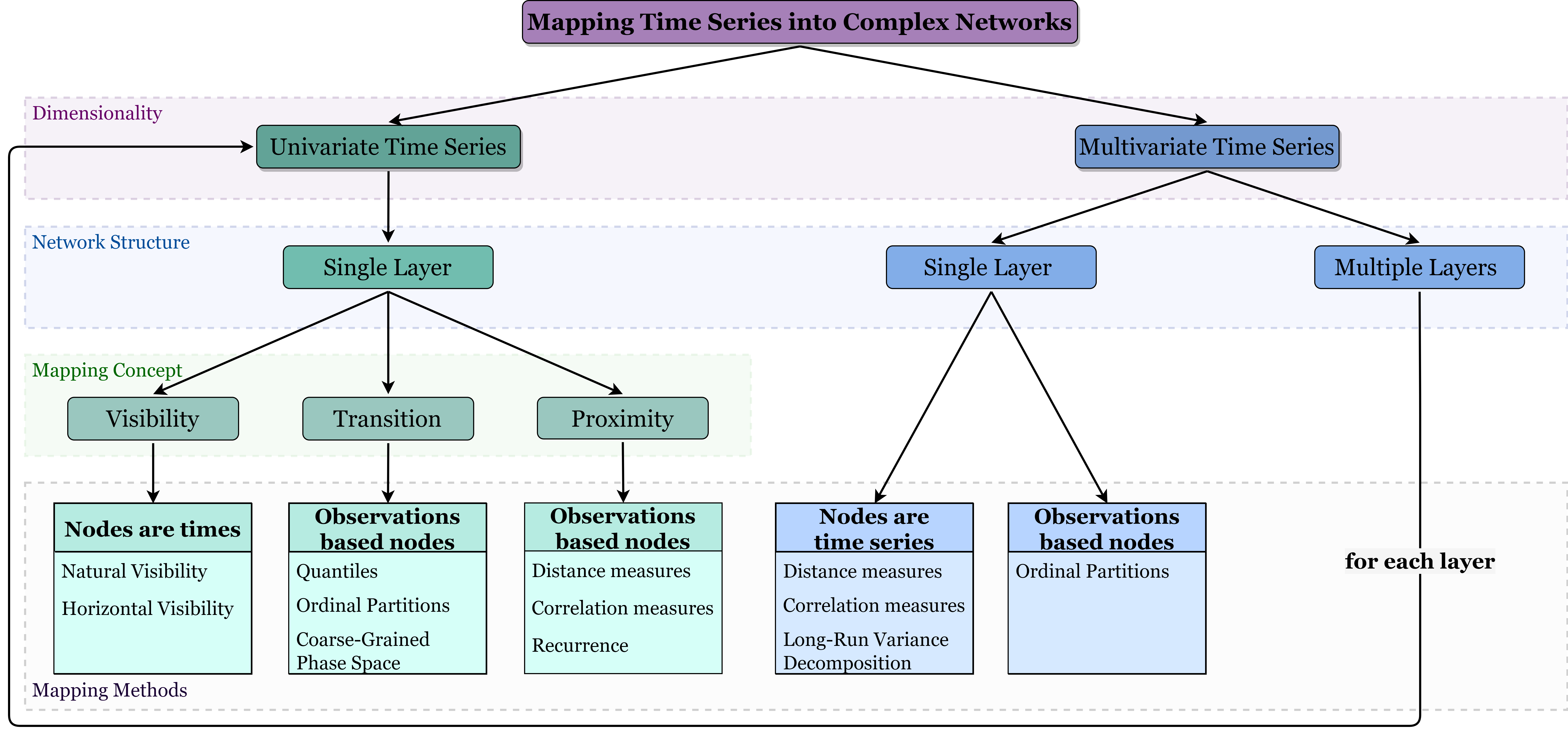
The set of univariate series mappings proposed in the literature may be divided into three main types depending on the underlying concept: visibility, transition and proximity. Visibility mapping concepts establish connections (edges) between the time stamps of the series (as nodes) using visibility lines (with or without restrictions) between observations. For transition mappings, the methods are based on the transition probabilities between states (or partitions) defined by dividing the time space in a set of temporal states (or dividing the series support/observations into partitions) that will be the nodes of the network. Finally, proximity mappings establish connections using measures of distance or similarity between time points (or states) become network nodes. Regarding multivariate time series, there are methods leading to a single layer network, where each series (or patterns based on observations from multivariate series) is represented by a node in the network and the connections are established based on relationships between the series (or patterns). We can also find mappings leading to multiple layer network structures, where each layer represents a time series and, in fact, each layer can be mapped based on one of the univariate time series mapping methods, separately. Research on multivariate mappings is however still in its infancy.

We aim at reaching a wide community of researchers and practitioners who may benefit from these methods in machine learning, data mining and time series analysis tasks. With this purpose in mind, the mappings are described from an algorithmic point of view geared towards software implementations. We provide quick reference tables summarizing the algorithms, properties of the mappings (univariate and multivariate) and of the resulting networks. Each mapping algorithm is depicted using a toy time series (the same for all methods for comparison purposes) to facilitate its understanding. In comparison to the survey by Zou et al., (2019), whose focus is on non-linear time series analysis by means of complex network methods, we add more recent aspects of the literature as well as approaches stemming from the statistical literature.

Given the multidisciplinary of time series, as well as complex networks, our approach in this review can impact several fields and provide new insights and structured information to practitioners of several areas.

2 Preliminaries

This section presents the background concepts and terminology on time series and network science and establishes the necessary notation for the remainder of the document.

2.1 Time Series

Formally, a time series $\boldsymbol{Y}=(Y_{1},\ldots,Y_{T})$ is a finite realization of a stochastic process which is a sequence of random variables $\{Y_{t}\}_{t}$ indexed by time $t$, or of a dynamic deterministic process that can be fully represented by an explicit mathematical relation. In this work we consider $t$ discrete and varying in the integers $t=0,\pm 1,\pm 2,\ldots.$ The main characteristic of a time series is the serial dependence between the observations which restricts the applicability of many conventional statistical methods developed under the assumption of independent and identically distributed (i.i.d.) observations. Time series analysis refers to the collection of procedures developed to systematically solve the statistical problems posed by the serial correlations. Thus, its main purpose is to develop mathematical models that provide plausible descriptions of data characteristics with a view to forecasting and simulation (Box et al.,, 2015).

A complete description of a time series $Y_{1},\ldots,Y_{T}$ is provided by the joint distribution function $F(c_{1},\ldots,c_{T})=P(Y_{1}\leq c_{1},\ldots,Y_{T}\leq c_{T})$. This joint distribution can be obtained easily only in the particular case of jointly Gaussian random variables and, even so, under the assumption of some regularity of the time series over time. Thus, time series analysis relies on a set of concepts and measures that capture the essential feature of the data, the serial correlation. The main statistical tools in time series analysis are the following. The mean function defined as $\mu_{t}=\mbox{\rm E}(Y_{t})$. The autocovariance function defined as the covariance between the variables at times $t$ and $s$:

$$\gamma(s,t)=\mbox{\rm cov}(Y_{s},Y_{t})=\mbox{\rm E}[(Y_{s}-\mu_{s})(Y_{t}-\mu_{t})],$$ (1)

for all $t$ and $s.$ We should note that $\gamma(s,t)=\gamma(t,s)$ for all-time points $s$ and $t$ and $\gamma(t,t)=\mbox{\rm E}[(Y_{t}-\mu_{t})^{2}]=\mbox{\rm var}(Y_{t}).$ The autocovariance measures the linear dependence between variables at different times. The autocorrelation function (ACF) which measures the linear predictability of the series at time $t$ using only the variable at time $s,$ $Y_{s},$ is defined as:

$$\rho(s,t)=\mbox{\rm corr}(Y_{t},Y_{s})=\frac{\gamma(s,t)}{\sqrt{\gamma(s,s)\gamma(t,t)}},$$ (2)

$-1\leq\rho(s,t)\leq 1$ with $\rho(s,t)=1$ indicating perfect positive correlation and $\rho(s,t)=-1$ indicating perfect negative correlation. Hence, the ACF provides a rough measure of the ability to forecast the series at time $t$ from the value at time $s$ (Shumway and Stoffer,, 2017).

The notion of regularity referred to above is defined using the concept of stationarity. Technically, we may distinguish strict (or strong) stationarity from weak (or wide, or second order) stationarity. A time series is said to be strictly stationary if the probabilistic behavior of every collection of variables $\{Y_{1},Y_{2},\ldots,Y_{t}\}$ is identical to that of the time shifted set $\{Y_{1+h},Y_{2+h},\ldots,Y_{t+h}\}$. However, this condition is too strong for most applications, and it is difficult to assess it for a single data set. Rather than imposing conditions on all possible distributions of a time series, weak stationarity imposes conditions only on the first two moments of the series. Thus, a time series is said to be weakly stationary if it is a finite variance process, with a constant mean function and does not depend on time $t$, $\mbox{\rm E}(Y_{t})=\mu$, and the autocovariance function depends only on the lag, $h=s-t$, $\gamma(s,t)=\gamma(s-t,0)=\gamma(h)$.

In summary, a time series is stationary when its statistical characteristics (mean and variance) are constant over time, that is, data fluctuate around a constant mean with the variance of the fluctuations remaining essentially the same over time. Moreover, stationarity implies that correlation between observations depends only on the time lag between the observations. Stationarity is essential in the analysis of time series since it enables the meaningful computation of statistics such as the mean, variance and ACF from the data.

The simplest time series process is the white noise (or purely random) process, henceforth denoted by $\epsilon_{t}.$ It is a sequence of i.i.d. random variables with mean $0$ and constant variance $\sigma_{\epsilon}^{2}.$ A particular case is the Gaussian white noise, where $\epsilon_{t}$ are independent normal random variables.

Univariate time series relate to measurements of a given variable over time, $Y_{t}$, such as temperature measurements. However, it is increasingly common to observe data from several variables, $Y_{i,t},$ $i=1,2,\ldots,m$, that may be correlated. For example, in air pollution studies atmospheric variables such as temperature and air humidity, as well as pollutants, such as particulate matter and NO₂ hourly concentrations are observed and need to be analyzed jointly and over time. We represent these multivariate time series by a vector, $\boldsymbol{Y}_{t}=[Y_{1,t},Y_{2,t},\ldots,Y_{m,t}]^{{}^{\prime}}$ where ^′ represents the transpose of a matrix/vector and $Y_{i,t}$ is the $i$-th component time series (a random variable for each $i$ and $t$).

Multivariate time series present not only serial dependence within each component series $Y_{i,t}$ but also interdependence between the different components $Y_{i,t}$ and $Y_{j,s}$ when $i\neq j$, regardless of whether the times $s$ and $t$ are the same or not. Although the theory of univariate time series extends in a natural way to the multivariate case new concepts arise. The $m$-dimensional time series process, $\boldsymbol{Y}_{t}$, is a stationary process if each of its component series is a univariate stationary process and the covariance matrix function depends only on the lag. Thus, $\mbox{\rm{E}}\left(\boldsymbol{Y}_{t}\right)=\boldsymbol{\mu},$ is now a $m$ vector of constants, and the autocovariance function, now a matrix function, is defined for lag $h$ as the $m\times m$ matrix $\Gamma_{\boldsymbol{Y}}(h)=\mbox{\rm{E}}\left[\left(\boldsymbol{Y}_{t}-\boldsymbol{\mu}\right)\left(\boldsymbol{Y}_{t+h}-\boldsymbol{\mu}\right)^{{}^{\prime}}\right]$, with elements $\gamma_{i,j}(h)=\mbox{\rm{cov}}(Y_{i,t},Y_{j,t+h})$. Note that $\Gamma_{\boldsymbol{Y}}(h)=\Gamma_{\boldsymbol{Y}}^{{}^{\prime}}(-h)$ and the element $(i,j)$ of matrix $\Gamma_{\boldsymbol{Y}}(0)$ is the contemporaneous correlation between $Y_{i,t}$ and $Y_{j,t}$ (see Wei,, 2019 for more details). Similarly, we can define the correlation matrix at lag $h$ with elements $\rho_{i,j}(h)=\mbox{\rm corr}(Y_{i,t},Y_{j,t+h}).$

The simplest example of an $m$-dimensional vector process is the vector white noise process, $\{\boldsymbol{a}_{t}\},$ with mean vector $0$ and covariance matrix function $\boldsymbol{\Sigma}$, where $\boldsymbol{\Sigma}$ is an $m\times m$ symmetric positive definite matrix. Although the components of the white noise process are serially uncorrelated $\mbox{\rm corr}(a_{i,t},a_{i,s})=0,$ for $t\neq s$, they may be contemporaneously correlated, $\mbox{\rm corr}(a_{i,t},a_{j,t})\neq 0$. The most common vector white noise process is the Gaussian white noise process for which $\boldsymbol{a}_{t}$ follows a multivariate normal distribution (Wei,, 2019).

The analysis of multivariate time series requires tools, methods and models for processing information contained in multiple measurements that have both temporal and cross-sectional dependence which must be necessarily different from standard statistical theory and methods based on a random sample that assume independence. Linear and non-linear models for multivariate time series have often been developed tailored to model data from specific areas and under several assumptions. In recent years, procedures to analyze high dimensional time series have been developed but many issues remain open (Wei,, 2019).

2.2 Network Science

Many real world systems can be seen as complex systems with a set of elements that interact with each other and which exhibit emergent collective properties (Costa et al.,, 2011). Graphs provide a powerful and general abstraction for this kind of scenarios, in which the elements are represented by nodes and the interactions by edges. Such graphs are often described as complex networks, since they typically exhibit non-trivial topological properties, due to the characteristics of the underlying complex system, which are neither random nor purely regular (Albert and Barabási,, 2002).

2.2.1 Graph Terminology and Concepts

A graph, $G$, is an ordered pair $(V(G),E(G))$, where $V(G)$ represents the set of nodes (or vertices) and $E(G)$ the set of edges (or links) between pairs of elements of $V(G)$. The number of nodes, also known as the size of the graph, is written as $|V(G)|$ and the number of edges as $|E(G)|.$ Two nodes $v_{i}$ and $v_{j}$ are neighbors (or adjacent) if they are linked, that is, if $(v_{i},v_{j})\in E(G).$ We can distinguish between directed edges, which connect a source node to a target node, and undirected edges, when there is no such concept of orientation. In the first case the graph is called directed or digraph. A graph is weighted, if there is a weight (or cost) $w_{i,j}$ associated the edge $(v_{i},v_{j}).$ It is classified as simple if it does not contain multiple edges (two or more edges connecting the same pair of nodes) and it does not contain self-loops (an edge connecting a node to itself). Figure 2 illustrates the concepts here defined and depicts a simple directed graph and a simple undirected weighted graph, respectively.

(a) Directed graph

(b) Undirected weighted graph

Figure 2: A representation of (a) a simple directed graph and (b) a simple undirected weighted graph.

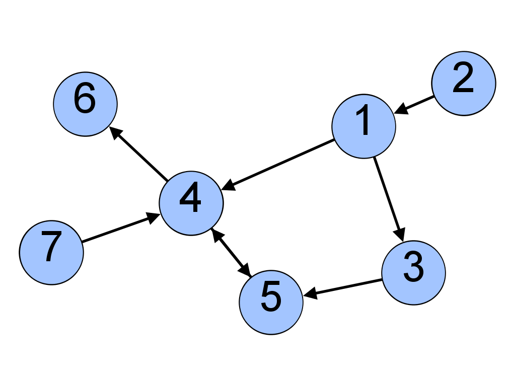
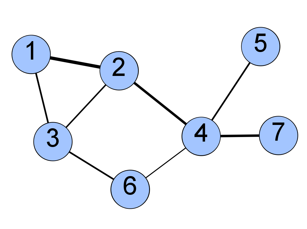
A graph $G$ is usually represented mathematically as an adjacency matrix denoted as $\boldsymbol{A}$, and $A_{i,j}$ is $1$ (or $w_{i,j}$) when $(v_{i},v_{j})\in E(G)$ and is $0$ otherwise. In the context of this paper, all nodes are labeled with consecutive integer numbers starting from $1$ to $|V(G)|$.

Most topological measures/metrics are related to the concepts of paths and graph connectivity. A path is a sequence of nodes in which each consecutive pair of nodes in the sequence is connected by an edge. It may also be useful to think of the path as the sequence of edges that connect those nodes. Two nodes are connected if there is a path between them and are disconnected if no such path exists. A set of nodes is called a connected component if all its node pairs are connected.

The analysis of complex networks has made enormous progress in the last decade, leading to the development of statistical properties of certain types of complex systems that are related and codified in their topology (Albert and Barabási,, 2002; Newman,, 2003). There exists therefore a vast set of topological metrics that are able to characterize a network, each reflecting some particular features of the system under analysis. A more detailed list of the most important topological metrics can be found in the literature (Albert and Barabási,, 2002; Costa et al.,, 2007; Barabási,, 2016).

2.2.2 Multilayer Networks

Most real world complex systems are not isolated and interact with other systems. Furthermore, a single entity may belong to several subsystems, establishing both internal (in the same system) and external (with other systems) connections. The latter type of connectivity can be interpreted as an interaction between levels (or layers), leading to the concept of multilayer networks.

A multilayer network is defined as a quadruplet $M=(V_{M},E_{M},V,\boldsymbol{L})$ where $\boldsymbol{L}=\{L_{a}\}^{s}_{a=1}$ are sets of elementary layers (that is, there is one set of elementary layers $L_{a}$ for each aspect $a$, $s$ is the number of aspects), $V$ is a set of nodes of $M,$ $V_{M}\subseteq V\times L_{1}\times\ldots\times L_{s}$ is a set of the node-layer combinations in which a node is present in the corresponding layer, and $E_{M}\subseteq V_{M}\times V_{M}$ is a set of edges that contains the pairs of possible combinations of nodes and elementary layers (Kivelä et al.,, 2014). A general simple representation of a multilayer network of two aspects can be seen in Figure 3a. Two particular cases of multilayer networks are the monoplex network, when $s=0$ and the multilayer reduces to a single-layer graph; and the multiplex network, when $M$ is a sequence of $l$ graphs, $\{G_{\alpha}\}_{\alpha=1}^{l}=\{(V_{\alpha},E_{\alpha})\}_{\alpha=1}^{l}$, where, usually, the node sets are the same across the different layers and the connections between nodes of different layers is only to its counterparts (Boccaletti et al.,, 2014); an example representation of a multiplex network can be seen in Figure 3b.

(a) Multilayer Network $(s=2)$

(b) Multiplex Network $(s=1)$

Figure 3: An example of a general (a) multilayer network with five nodes $V=\{0,1,2,3,4\}$ and two aspects, which have the corresponding elementary-layers sets $L_{1}=\{A,B\}$ and $L_{2}=\{X,Y\}$; (b) multiplex network with five nodes $V=\{0,1,2,3,4\}$ and one aspect. In both figures, solid lines represent intra-layer edges and dashed lines represent inter-layer edges.

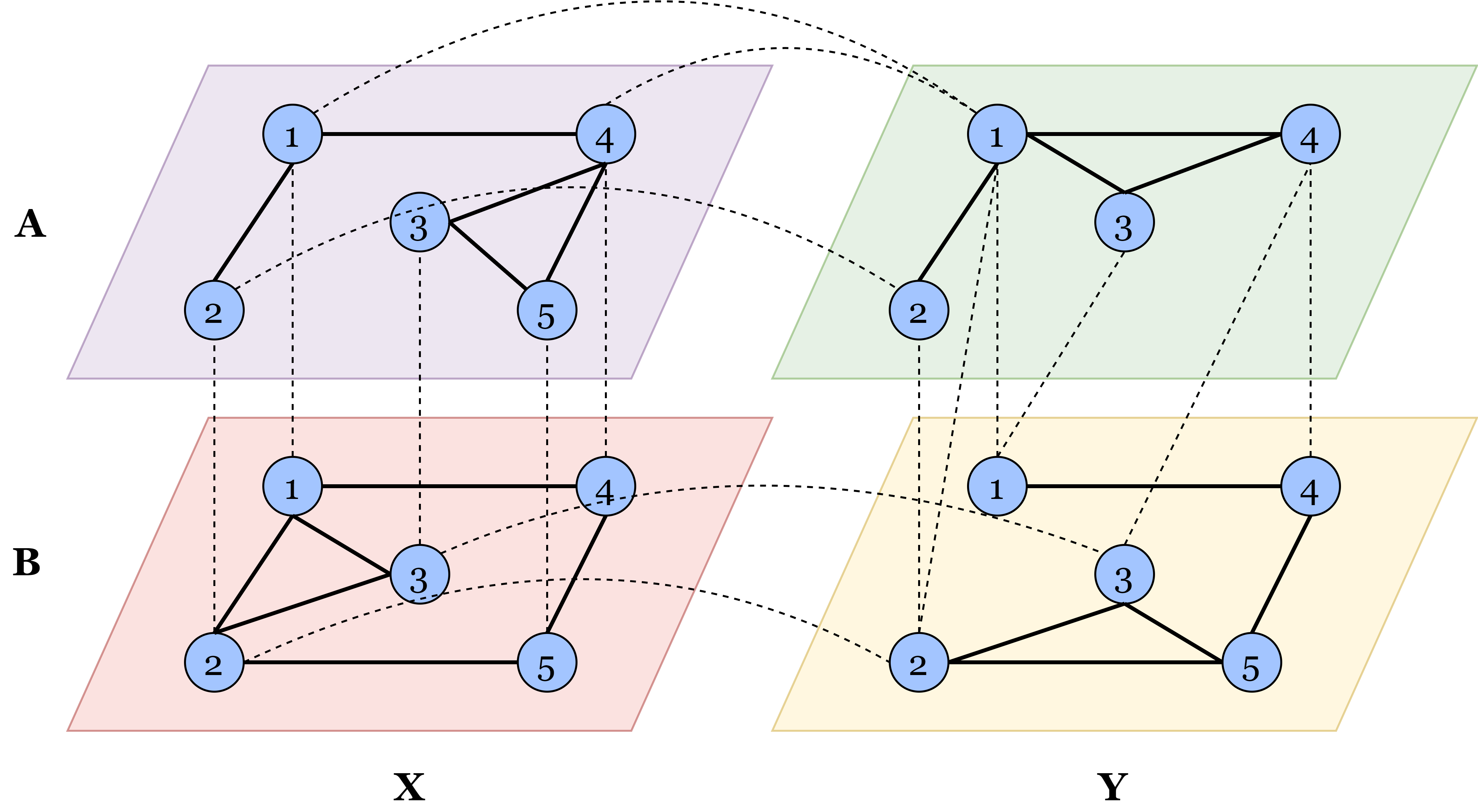
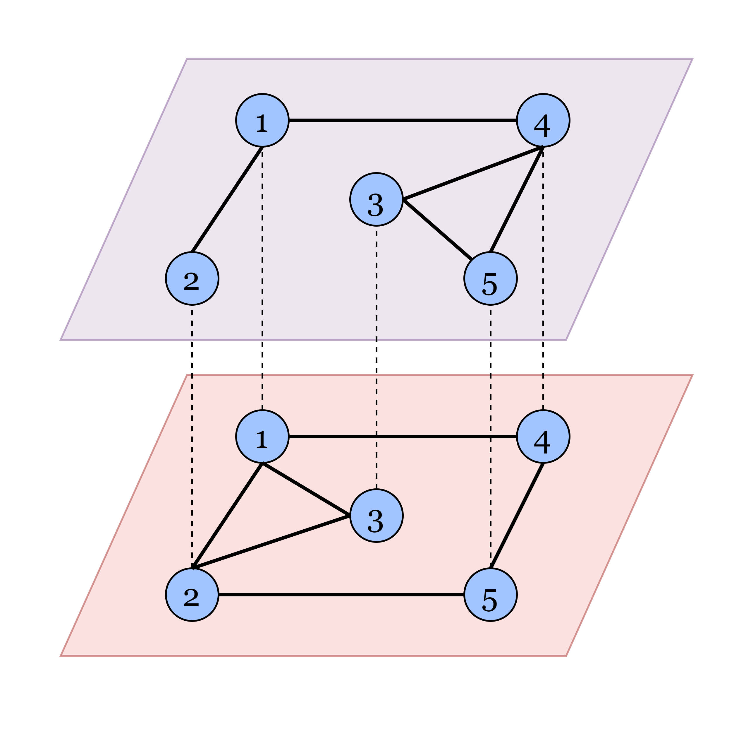
An unweighted multilayer network with $s$ aspects and the same number of nodes in each layer has an associated adjacency tensor $\mathcal{A}$ of order $2(s+1)$. Analogous to the adjacency matrix, each directed edge in $E_{M}$ is associated with a $1$ (or a weight $w$) entry of $\mathcal{A}$ (or two entries in undirected edges case) and the other entries are $0.$ If the network does not have the same number of nodes in each layer, we can consider empty nodes to complete (Porter,, 2018). Another representation is flattening $\mathcal{A}$ into a supra-adjacency matrix $\boldsymbol{A}$, where intra-layer edges are associated with entries on the diagonal blocks and inter-layer edges are associated with matrix entries on the off-diagonal blocks.

The analysis of multilayer networks is still a recent and not very mature topic, with most of the research being applied to networks with a single aspect (i.e., $s=1$), and in the context of multiplex networks (Kivelä et al.,, 2014; Porter,, 2018).

3 Mapping Univariate Time Series into Complex Networks

In this section, we review the state of the art of univariate time series mappings into the network domain. As previously represented in Figure 1, from a high-level perspective, and as in previous papers (Donner et al., 2011b, ; Zou et al.,, 2019), we divide the existing approaches into three different main classes, according to the underlying mapping concept. An overview of the main characteristics of the methods here described is given in Table 1. In the following sections we will give an in-depth description of how these approaches emerged, how they work, what variants exist, and what are the core results.

	Network Type (original reference)	Node	Edge	Directed	Weighted	Param-free	Pre proc
Visibility	Natural Visibility Network	$t$	NV	✗	✗	✓	✗
	(Lacasa et al.,, 2008)
	Horizontal Visibility Network	$t$	HV	✗	✗	✓	✗
	(Luque et al.,, 2009)
	Direct Horizontal Visibility Network	$t$	HV	✓	✗	✓	✗
	(Lacasa et al.,, 2012)
	Limited Penetrable Natural Visibility Network	$t$	NV	✗	✗	✗	✗
	(Zhou et al.,, 2012)
	Parametric Natural Visibility Network	$t$	NV	✓	✓	✗	✗
	(Bezsudnov and Snarskii,, 2014)
	Difference Visibility Network	$t$	V	✗	✗	✓	✗
	(Zhu et al.,, 2014)
	Weighted Visibility Network	$t$	NV	✓	✓	✓	✗
	(Supriya et al.,, 2016)
	Limited Penetrable Horizontal Visibility Network	$t$	HV	✗	✗	✗	✗
	(Gao et al., 2016a, )
Transition	Coarse-Grained Phase Space Network	$\vec{z}_{i}$	TP	✓	✓	✗	PS
	(Gao and Jin,, 2009)
	Quantile Network	$q_{i}$	TP	✓	✓	✗	DS
	(Campanharo et al.,, 2011)
	Ordinal Partitions Network	$\pi_{i}$	TP	✓	✓	✗	AR
	(Small,, 2013)
	Visibility Graphlets Network	$G_{i}$	TP	✓	✓	✓	PS;VG
	(Mutua et al.,, 2015)
Proximity	Cycle Network	$c_{i}$	CM	✗	✗	✗	DC
	(Zhang et al.,, 2006)
	Correlation Network	$\vec{z}_{i}$	CM	✗	✓	✗	PS
	(Yang and Yang,, 2008)
	$\kappa$-Nearest Neighbor Network	$\vec{z}_{i}$	DM	✓	✗	✗	PS
	(Small et al.,, 2009)
	Adaptive Nearest Neighbor Network	$\vec{z}_{i}$	DM	✗	✗	✗	PS
	(Xu et al.,, 2008; Small et al.,, 2009; Donner et al., 2011b, )
	$\epsilon$-Recurrence Network	$\vec{z}_{i}$	DM	✗	✗	✗	PS
	(Donner et al.,, 2010)

Table 1: Comparison of (univariate) time series mappings based on the properties of the corresponding algorithms and of the resulting networks. Notation: NV - natural visibility, HV - horizontal visibility, V - natural and horizontal visibility, TP - transition probability, CM - correlation measures, DM - distance measures, PS - phase space reconstruction, DS - division of the support, AR - amplitude rank, VG - directed visibility graph, DC - division into cycles.

3.1 Visibility Networks

Lacasa and co-authors (Lacasa et al.,, 2008) proposed visibility mappings from (univariate) time series to complex networks, based on traditional visibility algorithms from computational geometry (Ghosh,, 2007). The visibility networks have a geometric criterion associated with the natural ordering of the time series. Given its ease of interpretation and implementation, this mapping quickly attracted the research community and several results as well as variants of these methods began to emerge. Visibility-based algorithms incorporate, as we shall see, global and local topological characteristics of the time series in the graph characteristics, are easy to implement, computationally fast, and, except for the limited and parametric versions, are parameter-free.

Throughout this section we present the different types of visibility algorithms proposed in the literature, which are essentially based on the natural visibility (Lacasa et al.,, 2008) and horizontal visibility (Luque et al.,, 2009) algorithms.

3.1.1 Natural Visibility Graphs

Lacasa and co-authors (Lacasa et al.,, 2008) proposed the first method based on the concept of visibility, the natural visibility graph (NVG), or simply visibility graph (VG). This method is based on the idea that each observation of the time series is seen as a vertical bar with height equal to the numerical value of the observation and that these vertical bars are laid in a landscape, the top of a bar is visible from the tops of other bars. Each node in the graph corresponds to a time stamp $t$ of the time series, so the nodes are serially ordered. Two nodes are connected if there is a line of visibility between the corresponding data bars that is not intercepted. This idea is illustrated in Figure 4a.

(a) Toy time series

(b) NVG

Figure 4: On the left side, we present the plot of a toy time series and, on the right side, the network generated by the natural visibility algorithm. The purple lines in the time series plot represent the lines of visibility (and hence the edges of the graph) between data points.

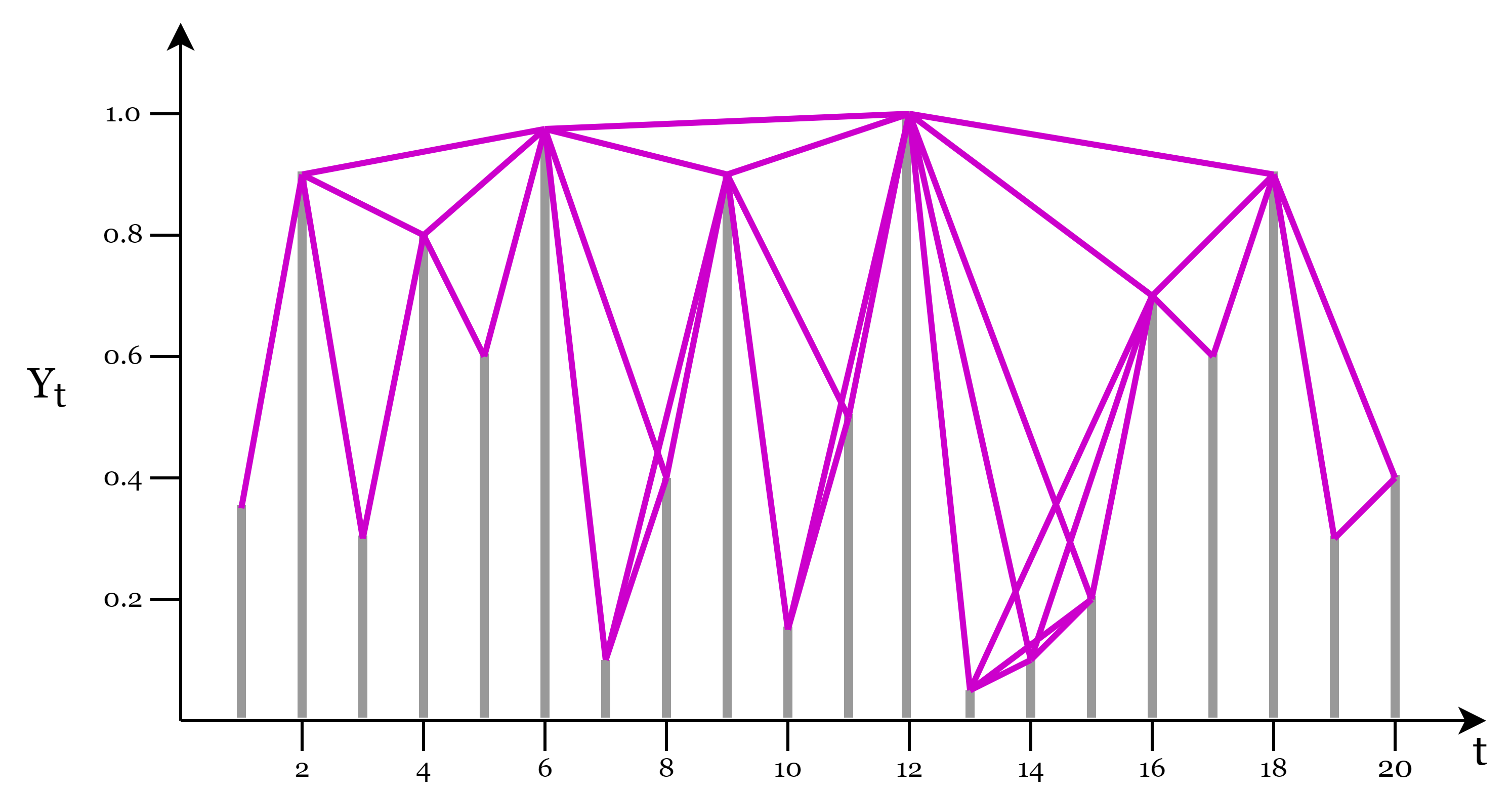
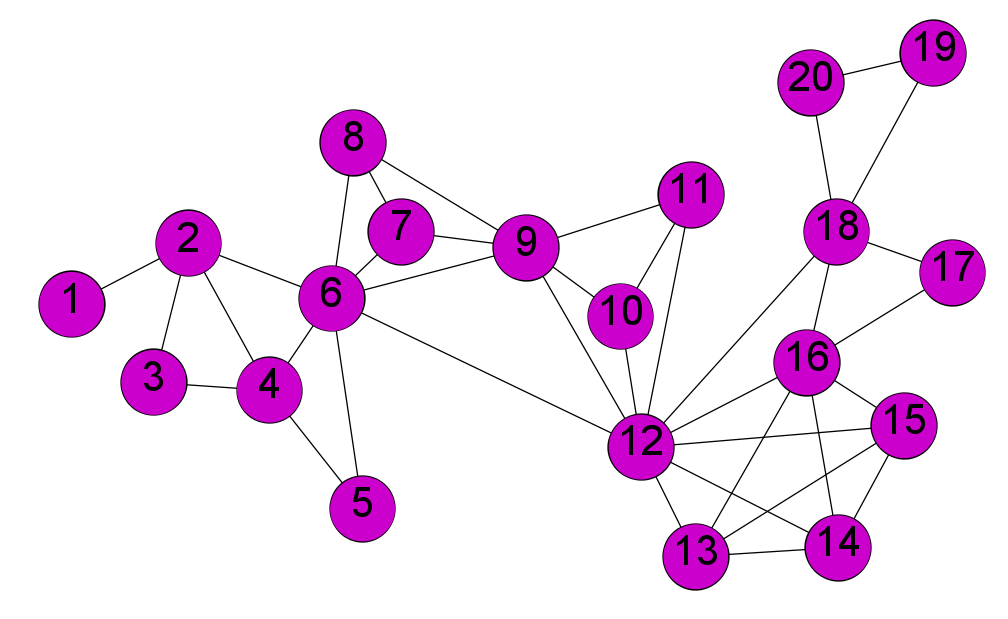
Formally, the set of nodes $\{v_{i}\}$ of a NVG are numbered sequentially in time and two nodes $v_{i}$ and $v_{j}$ are connected (have visibility) if any other observation $(t_{k},Y_{k})$ with $t_{i}<t_{k}<t_{j}$ satisfies:

$$Y_{k}<Y_{j}+(Y_{i}-Y_{j})\frac{(t_{j}-t_{k})}{(t_{j}-t_{i})}.$$ (3)

The NVG algorithm is easy to implement and, in terms of computational complexity, has quadratic complexity ($\mathcal{O}(T^{2})$) thus becomes very slow for very long time series. However, a more efficient algorithm based on the divide and conquer technique proposed in Lan et al., (2015) has a complexity of $\mathcal{O}(T\log T)$.

Visibility graphs are always connected because each node $v_{i}$ sees at least its neighbors, $v_{i-1}$ and $v_{i+1}$ and are always undirected. However, a direction can be defined considering the direction of the time axis. The network is also invariant under affine transformations of the data (Lacasa et al.,, 2008) because the visibility criterion is invariant under rescheduling of both the horizontal and vertical axis, as well as in vector translations, that is, each transformation $Y^{\prime}=aY+b,$ for $a\in\mathbb{R}$ and $b\in\mathbb{R},$ leads to the same NVG.

A NVG has, typically, a distinct topology characterized by hubs representing maxima of the time series, since these have visibility contact with more nodes when compared to other points (Donner and Donges,, 2012). However, this is not always necessarily true since a process with a concave behavior over a certain period of time, as for example the Conway series (Lacasa et al.,, 2008), can lead to highly connected nodes that do not coincide with local maxima (Donner and Donges,, 2012). The presence of hubs that correspond to (local) maxima of time series typically give rise to a topological structure represented by communities. These communities usually reflect the temporal order of the observations. The communities may also be formed by fragments of the time series, in which case do not reflect the temporal order of the observations (Yao and Lin,, 2017).

Lacasa and co-authors (Lacasa et al.,, 2008) have shown that NVGs inherit several structural properties of the time series. In fact, the method maps periodic series  on regular graphs, random series on random graphs  and fractal series on scale-free graphs . In particular, for periodic series, the graphs have a regular structure where the degree distribution presents a number of peaks related to the period of the series. For white noise processes the resulting graph is completely random, producing a degree distribution that is an exponential function. For fractal time series, the degree distribution is a power law related to the fractality of series.

In Lacasa et al., (2009), the authors used the NVGs to quantify long-range dependence and fractality in time series. These authors concluded that fractal processes result in scale-free visibility graphs with a degree distribution that is a power law $P(k)\sim k^{\gamma}$ with exponent $\gamma$ which is a linear function of the Hurst coefficient. These results were applied to study the fractality of energy dissipation rates in turbulent flows (Liu et al.,, 2010), to study turbulent heated jets behaviors (Charakopoulos et al.,, 2014) and to diagnose Alzheimer’s disease automatically based on the data electroencephalography (EEG) (Ahmadlou et al.,, 2010), among others.

Recently, a new definition of motif  in the context of NVG was presented in Iacovacci and Lacasa, 2016b : sequential NVG $n$-node motifs. According to this definition, motifs are the set of NVG subgraphs formed by the sequence of nodes $\{g,g+1,\ldots,g+n-1\}$, where $n<T$ and $g\in[1,T-n+1]$). This definition differs from traditional network motifs in that they require nodes to be labeled according to the temporal order of the nodes induced by the construction of NVG. One advantage of this definition is that the computation of these motifs is extremely efficient, linear time $\mathcal{O}(T)$, using the theory developed in Iacovacci and Lacasa, 2016a . Similarly to traditional motifs networks, we can compare the relative occurrence of each motif to distinguish different time series processes, see more details in Iacovacci and Lacasa, 2016b .

Donner and Donges (Donner and Donges,, 2012) address the problem of missing data in time series. They assessed the effect that missing data produces in the topological properties of NVGs associated with Gaussian white noise processes, using two strategies: missing data is simply ignored in the generation of the NVG; the NVG is fragmented into subgraphs corresponding to times before and after the missing observations. Donner and Donges, (2012) concluded that ignoring the missing data had a considerable effect mainly on closeness centrality but not on degree distribution and local clustering coefficient, as well. When the missing data is taken into account and the NVG becomes a set of subgraphs, path-based metrics are the most impacted. As expected the impacts become stronger as the missing data increases. Interestingly, those authors also found out that the effects of node-level metrics are slightly reduced for missing data occurring in runs rather than randomly.

Given the potential demonstrated, the method was applied in the study of energy dissipation rates in three-dimensional turbulence (Liu et al.,, 2010), financial time series (Yang et al.,, 2009; Qian et al.,, 2010; Long,, 2013; Zhuang et al.,, 2014), heart rate variability (Shao,, 2010; Hou et al.,, 2016), classification of sleep stages (Zhu et al.,, 2014), classification of time series (Li et al.,, 2018), hurricane occurrence in the United States (Elsner et al.,, 2009) and to perform forecasting (Zhang et al., 2017b, ; Zhang et al., 2018b, ).

Note that NVGs are not able to distinguish time series with certain traits. As an example, consider a time series with a deterministic increasing trend. Its NVG and the NVG of its symmetric time series which presents a deterministic decreasing trend are similar graphs with the same properties. This disadvantage may be overcome defining NVGs with directed edges.

3.1.2 Horizontal Visibility Graphs

In order to reduce the computational complexity associated with NVGs, Luque and co-authors (Luque et al.,, 2009) proposed a simplified NVG method called the horizontal visibility graph, HVG, which inherits all NVG graph characteristics mentioned above. The construction of HVGs differs from that of NVGs in that the visibility lines are only horizontal. Figure 5 gives a simple illustration of this algorithm, with a toy time series and the resulting network.

(a) Toy time series

(b) HVG

Figure 5: On the left side, we present the plot of a toy time series and, on the right side, the network generated by the horizontal visibility algorithm. The green lines represent the horizontal lines of visibility between the data points and the purple lines the natural visibility, to comparison.

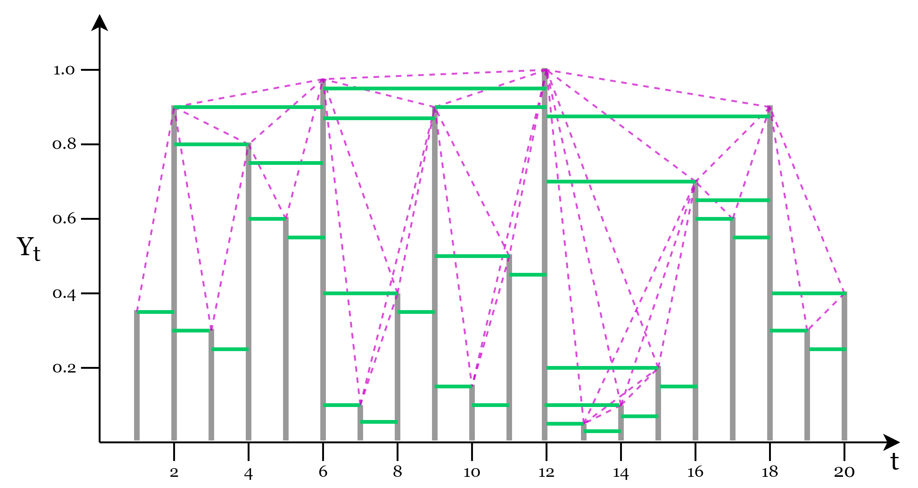
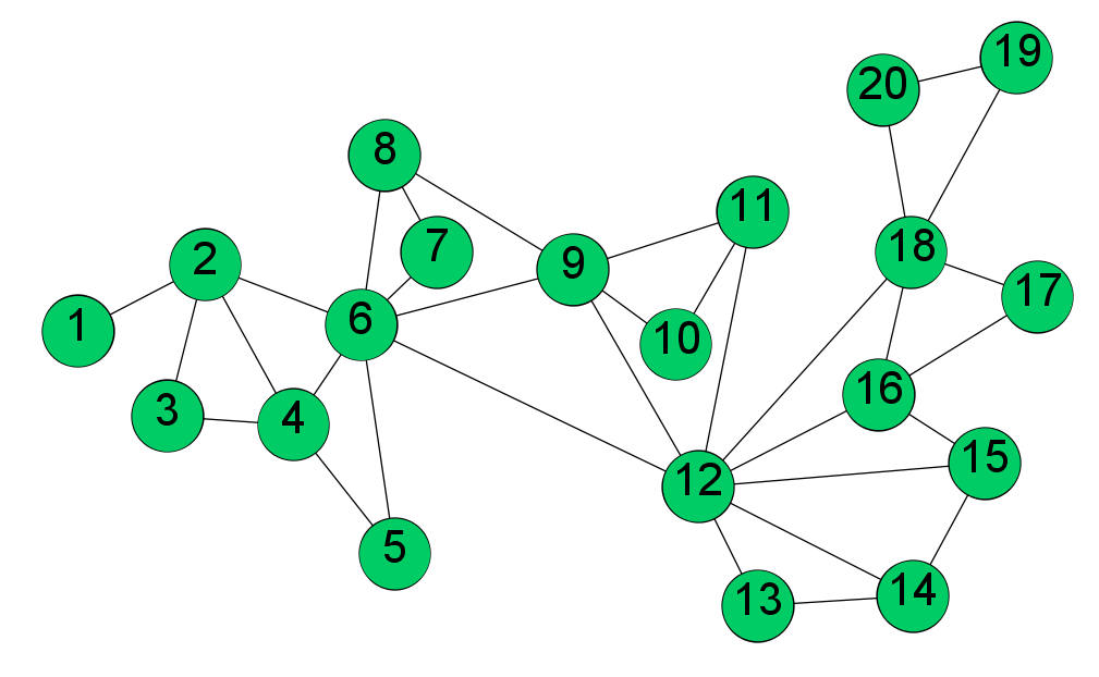
Formally, two nodes $v_{i}$ and $v_{j}$ are connected, if the following condition is met:

$$Y_{i},Y_{j}>Y_{k},$$ (4)

for all ($t_{k},Y_{k})$ such that $t_{i}<t_{k}<t_{j}$.

In terms of computational complexity, the generation of HVGs has time complexity of the construction $\mathcal{O}(T\log T)$ (Yela et al.,, 2020) and, in the case of noisy (stochastic or chaotic) processes the algorithm has an average-case time complexity $\mathcal{O}(T)$ (Luque et al.,, 2009).

The HVG is always a subgraph of the NVG for a particular time series. This is well illustrated in Figures 4 and 5 where we can easily verify that all the edges present in the HVG are present in NVG, but the converse is not true, e.g. edges $(6,8)$ and $(12,15).$ HVG nodes will always have a degree less than or equal to that of the corresponding NVG nodes. Therefore, there is some loss of quantitative information in HVGs in comparison with NVGs (Luque et al.,, 2009) which may be crucial in the analysis of certain time series. However, it has no impact on the qualitative characteristics of the graphs, since the graphs preserve some part of the data information, namely the local information (the closest time stamps). Another characteristic of HVGs is that it is always an outerplanar graph  and has a Hamilton path, that is, a path that passes through all the nodes of a graph only once. In fact, Gutin et al., (2011) have shown that this is a necessary and sufficient condition for a graph to be an HVG.

Luque and co-authors (Luque et al.,, 2009) have formally established several relationships between properties of HVGs and characteristics of the underlying time series.

The first such property states that uncorrelated random series is mapped into an HVG with an exponential degree distribution given by:

$$P(k)=\frac{1}{3}\left(\frac{2}{3}\right)^{k-2},\quad\textrm{for }k\geq 2.$$ (5)

This result holds for all probability distributions. It follows that, for uncorrelated random series, the associated average degree is (Nuñez et al., 2012a, ):

$$\bar{k}=\sum kP(k)=\sum_{k=2}^{\infty}\frac{k}{3}\left(\frac{2}{3}\right)^{k-2}=4.$$ (6)

Additionally, Lacasa and Toral, (2010) suggested that the degree distribution follows the exponential law, $P(k)\sim\exp^{(-\lambda k)}$, where the value of $\lambda$ depends on the type of process generating the time series: $\lambda<\ln(\frac{3}{2})$ for chaotic processes, $\lambda>\ln(\frac{3}{2})$ for stochastic processes and $\lambda=\ln(\frac{3}{2})$ for uncorrelated processes. However, note that Ravetti et al., (2014) found that for the R$\ddot{\text{o}}$ssler system  the rule is not valid, and Zhang et al., 2017c found results in which negatively correlated processes lead to lower $\lambda$ values than the critical value. These results show that there are exceptions to the rule and that using $\lambda$ to distinguish chaotic from stochastic processes requires further investigation.

A second property obtained by Luque et al., (2009) refers to the relationship between hubs of the graph and the extreme values of the data. This equivalence was obtained numerically. Furthermore, based on geometric arguments, Luque et al., (2009) obtained the following relation between the clustering coefficient, a measure to capture the degree to which the nodes of a graph tend to cluster, and the degree in an HVG:

$$C_{i}=\frac{k_{i}-1}{\binom{k_{i}}{2}}=\frac{2}{k_{i}},$$ (7)

where $\binom{k_{i}}{2}$ denotes the number of possible triangles and $k_{i}-1$ is the number of visible nodes that are also visible from $v_{i}$. This relation allows also to deduce the local clustering coefficient distribution (Nuñez et al., 2012b, ), substituting $k_{i}$ by $C_{i}$ in Equation (5).

The HVG associated to an infinite periodic series of period $P$ is a representation of a concatenation of a motif. Nuñez and co-authors (Nuñez et al., 2012a, ) proved that the average degree of the resulting HVG is given by:

$$\bar{k}=4\left(1-\frac{1}{2P}\right).$$ (8)

This result implies that time series are mapped on HVGs with $2\leq\bar{k}\leq 4$. The lower bound is reached for constant series (HVG is a chain graph and so each node is only connected to its two closest neighbors) and the upper bound for aperiodic series (random and chaotic process).

Nuñez and co-authors (Nuñez et al., 2012a, ) proposed a method for calculating the hidden periodicity in a periodic noisy signal, a very common problem in real world data analysis and difficult to solve with traditional periodicity detection algorithms, such as spectral analysis. The method involves the construction of a modified HVG, called the filtered HVG (f-HVG), where two nodes $v_{i}$ and $v_{j}$ are connected if the following condition is meet:

$$Y_{i},Y_{j}>Y_{k}+f,$$ (9)

for all $t_{i}<t_{k}<t_{j}$ and $f\in[\min(Y_{t}),\max(Y_{t})]$ is a real-valued scalar that acts as a filter. To filter the noise of a time series, its f-HVG is generated for increasing values of $f$, and at each step, the average degree is calculated. The result is a decrease of the average degree, with initial value $4$ (for $f=0$), an asymptotic value of $2$ (lower bound of $\bar{k}$) and the plateau obtained for the distribution allows to obtain the period through Equation (8). This method delivered very promising results including, specific cases where autocorrelation analysis yields misleading results.

The definition of sequential motif presented for NVGs in Iacovacci and Lacasa, 2016b also apply similarly to HVGs. The definition of sequential HVG $n$-node motifs is the same way as that for an NVG. The frequency of sequential HVG motifs is also useful for discriminating different dynamic process.

HVGs were used to analyze seismic signals (Telesca and Lovallo,, 2012), evaluate the complex dynamics of tourism systems (Baggio and Sainaghi,, 2016), construct the so-called Feigenbaum graphs in order to study unimodal maps and their spectral properties (Flanagan et al.,, 2019), study the volatility behavior of returns for financial time series (Zhang et al.,, 2015), analyze heartbeat rates of healthy subjects, congestive heart failure subjects, and atrial fibrillation subjects (Xie et al.,, 2019) and predicting catastrophes (Zhang et al., 2018a, ).

In a recent work, Li et al., (2018) show that the topological properties of the NVGs and HVGs are useful features for constructing accurate classification models using generic classifiers for the classification of real time series, since combining both graphs allows capturing global (in the case of NVGs) and local (in the case of HVGs because they are more sensitive to local variations) features. This approach allows to increase the classification accuracy of a vast set of time series of different domains and it turns out to be better when compared to the traditional approaches, such as time series features obtained from common statistical measures.

Several variants of NVGs and HVGs have been proposed in the literature. The most relevant are presented in the following sections.

3.1.3 Directed Visibility Graphs

Given that time has a natural direction, Lacasa et al., (2012) introduced directed horizontal visibility graphs, DHVG, by defining an HVG with edges $(v_{i},v_{j})$, $i<j.$ The adjacency matrix is no longer a symmetric matrix. An example of the representation of this algorithm is illustrated in Figure 6. This variant is extended straightforwardly to the NVGs.

(a) Toy time series

(b) DHVG

Figure 6: Illustrative example of directed horizontal visibility algorithm and corresponding out-degree ($k_{i}^{out}$), in-degree ($k_{i}^{in}$) and total-degree ($k_{i}$). On the left side, we present the plot of a toy time series and, on the right side, the network generated by the directed horizontal visibility algorithm. The green directed lines represent the directed horizontal lines of visibility between data points.

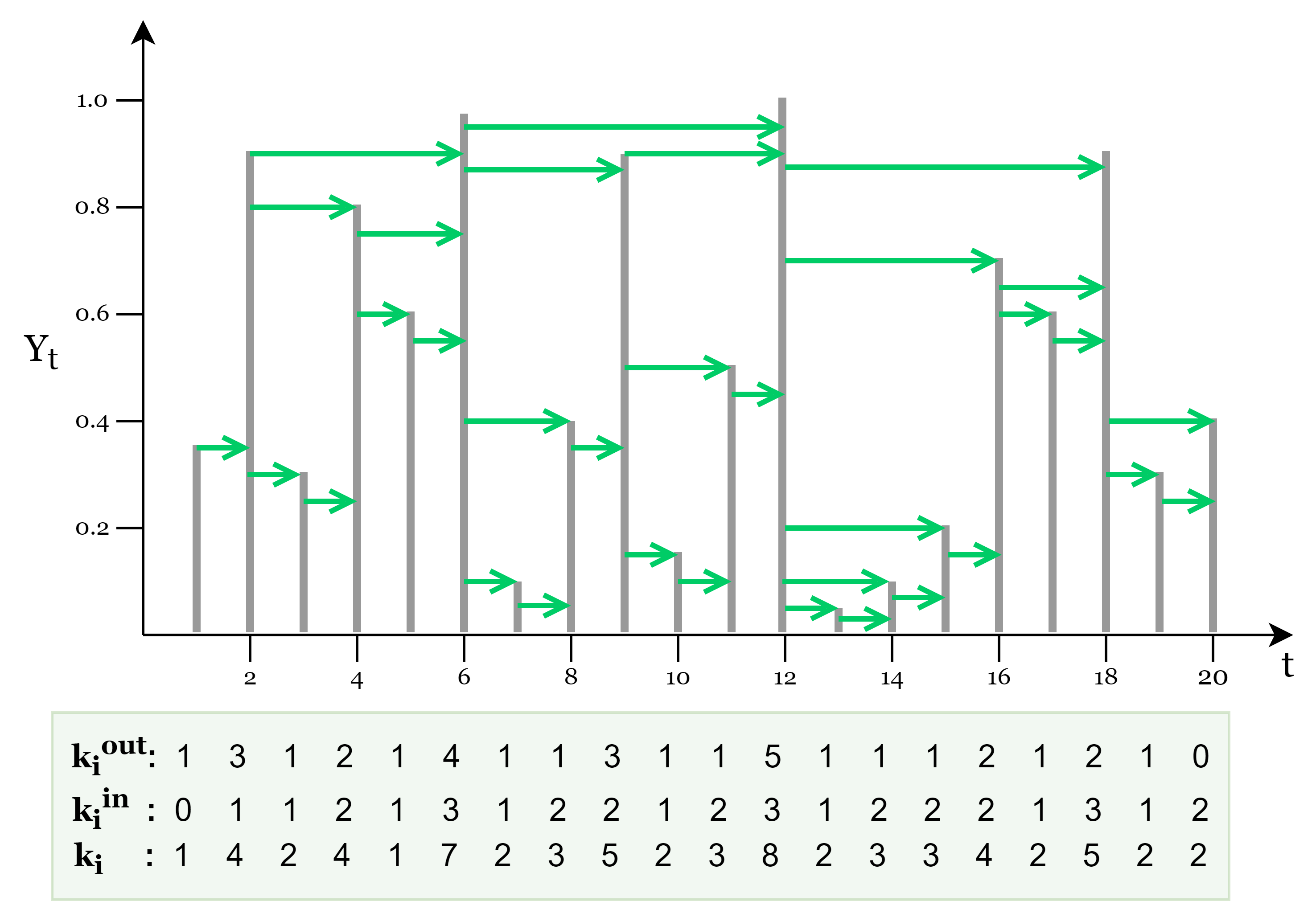
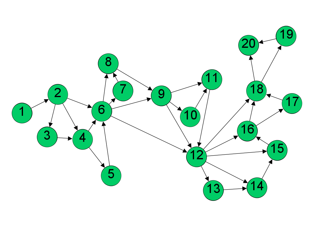
DHVG were proposed as a simple and well-defined tool for measuring time series irreversibility  notoriously difficult to assess with traditional algorithms, like algorithms that involve time series symbolization, which normally involve the choice of extra parameters and the results may depend on that choice. The degree of irreversibility of a time series is calculated as the Kullback-Leibler distance between the in- and out-degree distributions, $P(k^{in})$ and $P(k^{out})$ (Lacasa et al.,, 2012). These authors proved that for a bi-infinite sequence of i.i.d. random variables, both the in and out-degree distributions of the corresponding DHVGs are equal and given by:

$$P(k^{in})=P(k^{out})=\left(\frac{1}{2}\right)^{k},\quad k=1,2,3,\ldots.$$ (10)

In the same line of research Donges et al., (2013) followed a similar approach. Donges and co-authors proposed a set of rigorous statistical tests for time series irreversibility based on both visibility algorithms (NVG and HVG). The authors compare the degree and local clustering coefficient distributions taking into account the past ($P(k^{r})$ and $P(C^{r})$) and the future ($P(k^{a})$ and $P(C^{a})$) separately. It is conjectured that if a time series is reversible the distributions $P(k^{r})$ and $P(k^{a})$ (or $P(C^{r})$ and $P(C^{a})$) should be similar, while for irreversible time series we should find statistically significant deviations between the distributions.

3.1.4 Limited Penetrable Visibility Graphs

The limited penetrable visibility graph, LPVG, was first proposed by Zhou et al., (2012) to improve the NVG and HVG mappings. Similarly to the NVG method, the nodes are numbered sequentially in time but now have a limit $l$ of visibility and the nodes $v_{i}$ and $v_{j}$ are connected if:

$$Y_{i+l}<Y_{j}+(Y_{i}-Y_{j})\frac{t_{j}-(t_{i}+t_{l})}{(t_{j}-t_{i})},\quad l<j-i,$$ (11)

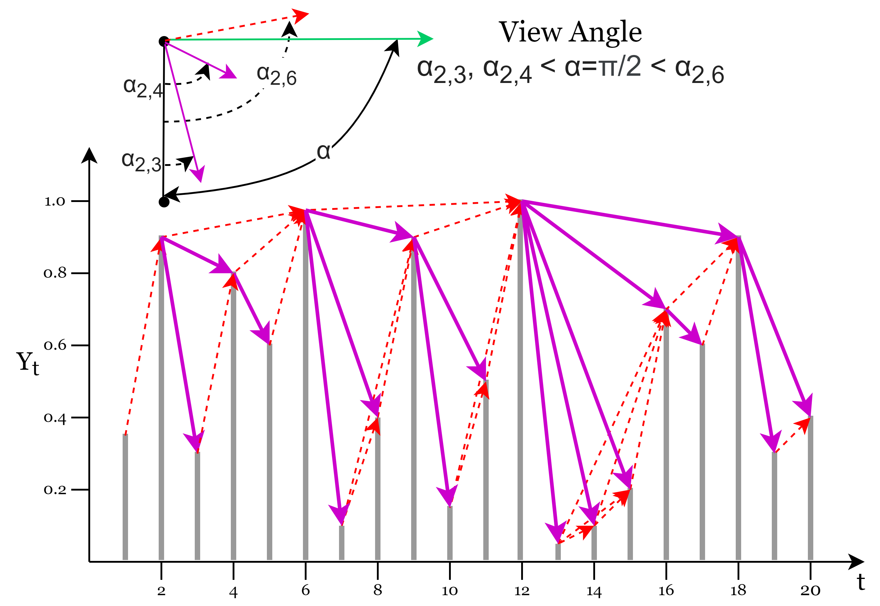
where $l$ is a limited penetrable distance established to reduce the effect of noise intrinsic to data. So, the nodes $v_{i}$ and $v_{j}$ have mutual visibility through $l$ intermediate bars (data) in the time series. The presence of noise in the data causes the connections on NVGs to break easily, while the nodes should, in principle, have more connections to other nodes, except for the maxima data (Pei et al.,, 2014). A small illustration of this method for $l=1$ is represented Figure 7a.

(a) LPVG algorithm

(b) PNVG vs. DNVG algorithm

Figure 7: (a) Illustrative example of limited penetrable visibility graph algorithm where the limit $l=1$. The purple lines show the edges between points that have direct visibility (as in NVG, $l=0$) and the blue dashed lines are the extra edges imposed by LPVG algorithm, where two points can be seen with only one higher intermediate point. (b) Illustrative example of parametric natural visibility graph algorithm with comparison with NVG algorithm.

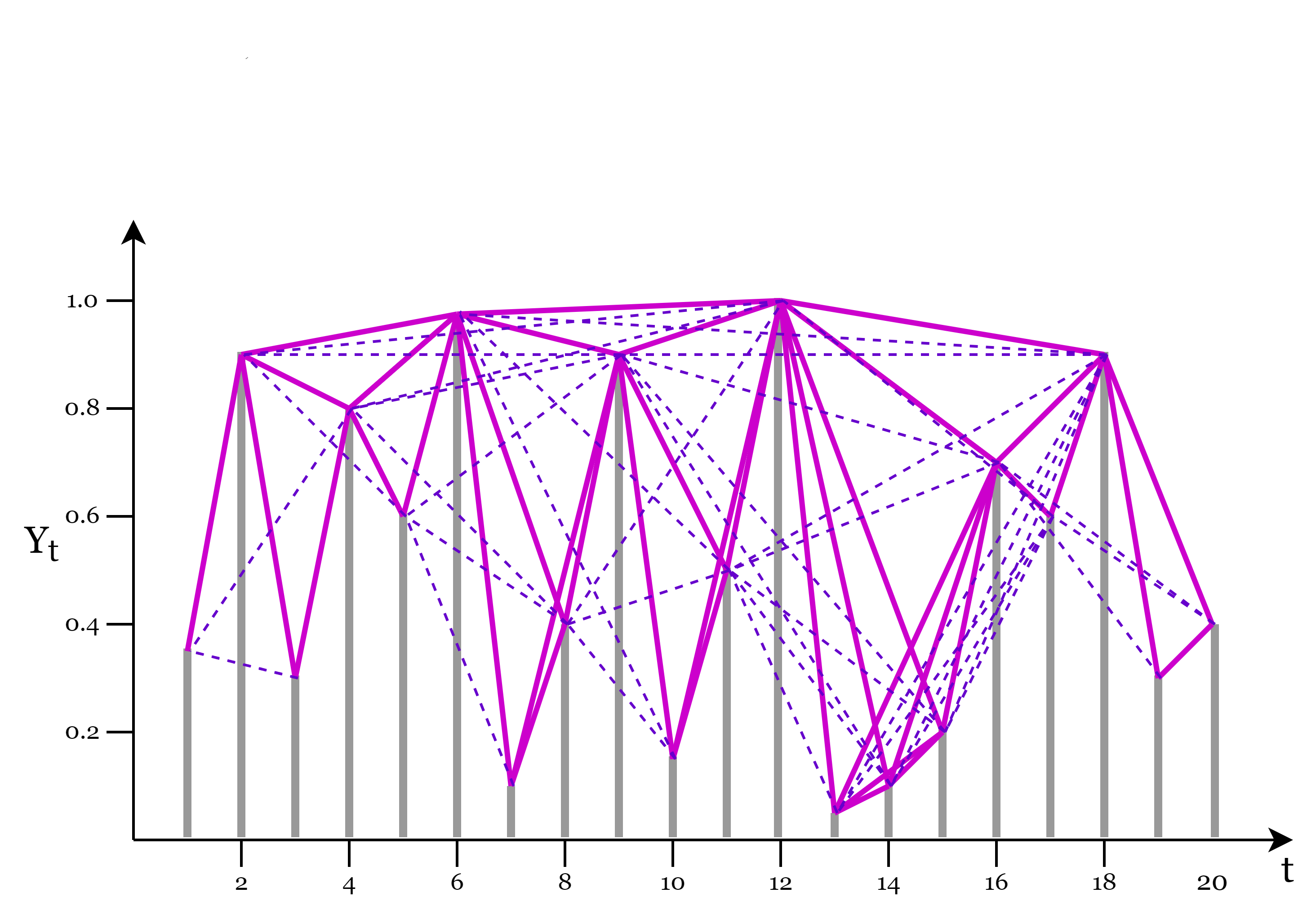
A limited penetrable version for HVG was developed by Gao et al., 2016a , and called limited penetrable horizontal visibility graph (LPHVG). The graphs are constructed using the above algorithm, except that the visibility condition is horizontal visibility. Note that when $l=0$, the LPVG (LPHVG) is reduced to NVG (HVG). Other versions of this method exist, namely, a directed version, the directed limited penetrable horizontal visibility graph (DLPHVG), and an image version, the image limited penetrable horizontal visibility graph (ILPHVG) (Wang et al., 2018b, ).

LPVGs are very promising: as the NVGs they inherit several properties of the time series and are able to detect differences between random and chaotic series, detect the location of inverse bifurcations in chaotic dynamical systems and, in addition, as an advantage over NVGs, they show good tolerance to noise interference (Wang et al., 2016a, ). However, it is necessary to pay attention to the choice of parameter $l$ so that not too much information is incorporated in the graphs.

The idea of limited natural visibility was applied to analyze abnormalities of EEG signals from Alzheimer’s disease (Wang et al., 2016a, ), EEG signals under manual acupuncture (Pei et al.,, 2014), and signals from an electromechanical system in the process industry (Wang et al., 2016b, ).

Ren and Jin (Ren and Jin,, 2020) applied the idea of sequential motifs (see Subsection 3.1.1) to LPVGs and introduced a measure of motif entropy to estimate the complexity of network structure, rather than looking at the motif occurrence frequency. They obtained a better robustness and the ability to distinguish different processes when compared to visibility-graph motif entropy.

Wang et al., 2018a presents some exact results (similar to those obtained for the HVGs presented in Subsection 3.1.2) on the topological properties of the LPHVG associated with bi-infinite time series of i.i.d. random variables with a probability density $f(x)$. The degree distribution of the associated LPHVG with the limited penetrable distance $l$ is given by:

$$P(k)=\frac{1}{2l+3}\left(\frac{2l+2}{2l+3}\right)^{k-2(l+1)},$$ (12)

where $l=0,1,2,\ldots,$ and $k$ is the degree of a node. From Equation (12) we obtain the average degree $\bar{k}$:

$$\bar{k}=\sum kP(k)=4(l+1).$$ (13)

And based on the Equation (12) we can deduce the minimum and maximum local clustering coefficient of the LPHVG associated to i.i.d. random series as (see Wang et al., 2018a for more details):

$$C_{min}(k) = \frac{2}{k}+\frac{2l(k-2)}{k(k-1)},\quad l=0,1,2,\ldots;\quad k\geq 2(l+1)$$ (14)

$$C_{max}(k) = \frac{2}{k}+\frac{4l(k-3)}{k(k-1)},\quad l=0,1,2,\ldots;\quad k\geq 2(2l+1).$$ (15)

For an infinite periodic series of period $P$ the average degree depends on the period $P$:

$$\bar{k}=4(l+1)\left(1-\frac{2l+1}{2P}\right),\quad l\ll P.$$ (16)

LPHVG was employed in the analysis of EEG signals and biphasic-flow signals where they characterize the behaviors underlying the systems (Gao et al., 2016a, ), in the analysis of chaotic series and energy and oil price series (Wang et al., 2018a, ), and to distinguish between random, periodic and chaotic signals using motifs (Wang et al., 2018b, ).

3.1.5 Weighted Visibility Graphs

The method proposed by Supriya and co-authors (Supriya et al.,, 2016) is a fairly simple modification to the traditional NVG algorithm, it considers the NVG edges as directed and weighted. For a given time series the corresponding weighted visibility graph (WVG) (or weighted directed visibility graph, WDVG) is constructed as follows: a directed NVG is constructed as described in Subsection 3.1.3, and a weight $w_{i,j}$ equal to the view angle between the observations $(t_{i},Y_{i})$ and $(t_{j},Y_{j})$ in time series is assigned to the edge that connect the corresponding nodes. The angle is given by:

$$\alpha_{i,j}=\tan^{-1}\left(\frac{Y_{j}-Y_{i}}{t_{j}-t_{i}}\right),\quad i<j.$$ (17)

We should note that Equation (17) allows the attribution of not only positive weights but also negative weights to the edges of the WVG. However, the analysis of networks with negative weights is more complex, standard methods and techniques do not apply straightforwardly (Kaur and Singh,, 2016), and therefore is less common. For this reason, Supriya et al., (2016) consider the absolute value of the view angle ($|\alpha_{i,j}|$) between the observations of the time series. We can see that the sign of the angle between the observations is an indicator of an increase (positive angle) or decrease (negative angle) of the values of the underlying process, thus providing information about changes in trends throughout the series.

We can consider a parametric version of WVGs, called parametric natural visibility graph, PNVG or PNVG$(\alpha)$, proposed by Bezsudnov and Snarskii (Bezsudnov and Snarskii,, 2014). This algorithm adds a restriction to the edge assignment in WVG determined by a threshold parameter $\alpha$ associated with the visibility angle. So, the PNVG($\alpha$) imposes that an weighted edge $(v_{i},v_{j},w_{i,j})$ is established from node $v_{i}$ to node $v_{j}$ only if the view angle between those nodes is less than threshold parameter, that is, $\{(v_{i},v_{j},w_{i,j})\in E(G_{PNVG})\text{ }|\text{ }\alpha_{i,j}<\alpha,w_{i,j}=|\alpha_{i,j}|\}$, as shown in the Figure 7b.

The PNVG($\alpha$) is a directed acyclic graph, it is always a subgraph of the underlying NVG (and WVG) and, consequently, invariant under affine transformations of the time series; and it can be a connected or disconnected graph.

PNVG and WVG were designed to try to overcome the loss of quantitative information of the NVG’s binary matrix. Other than arc tangent weights can be associated to the edges of the graphs. The arc tangent is a direct measure of the concept of visibility and a direction for future work may be to analyze its properties. However, the characteristics of the resulting network will always be dependent on this weight.

Specific topological measures were defined for this mapping, namely, relative average degree, relative average length of edge and relative number of clusters, which aim to compare the average degree, average length of edges and number of clusters with the corresponding measures in the underlying NVG (i.e., when $\alpha=\pi$). The authors in Bezsudnov and Snarskii, (2014) showed that these measures are useful for distinguish, identify and describe various time series. They performed tests in different synthetic time series and in real heart rate data to distinguish different series associated with people with different health conditions, where they obtained good results. However, PNVG is not a parameter-free method and it always involves choosing the parameter $\alpha$ that conditions the final results.

In Supriya et al., (2016) the authors applied this approach to EEG reference data associated with epileptic activity and showed that the metrics such as modularity (that measures how good a division of the graph is in specific communities) and weighted average degree of WVG constructed for this data help to distinguish convulsion signals from normal signals, detecting the sudden fluctuations in signals. The accuracy of the results surpassed many other methods.

Note that other strategies for assigning weights to the edges of (natural or horizontal) visibility graphs, that are different from those of the visibility angles, can be considered. Examples include Bianchi et al., (2017) and Xu et al., (2018) leading to undirected and weighted horizontal and natural visibility graphs.

3.1.6 Difference Visibility Graphs

A variant of the NVG and HVG consists of the creation of difference visibility graphs, DVG (Zhu et al.,, 2014). This algorithm subtracts the HVG edge set from the NVG edge set. Thus, the degree $k_{i}$ of a node $v_{i}$ of the DVG is: $k_{i}=k_{i,NVG}-k_{i,HVG},$ since the HVG is always a subgraph of the NVG. For the average degree we have $\bar{k}=\bar{k}_{NVG}-\bar{k}_{HVG}$. DVGs will very possibly be disconnected and may have isolated nodes (which have no connections). The DVGs were used together with HVGs in Zhu et al., (2014); An et al., (2019) to extract graph metrics, as average degree, degree distribution and degree sequence, to classify automatically real EEG data in order to detect different sleep stages. DVGs obtained intermediate precision values when compared to other strategies (An et al.,, 2019).

3.2 Transition Networks

Transition networks are a type of networks that are constructed from time series based on the concept of transition between symbols that are assigned to represent the series. In general, the construction of transition networks involves two fundamental steps: assigning a symbol encoding to the time series data; mapping the symbols and the transition function between the symbols into the nodes and the edges, respectively. The first step transforms the time series into a set of symbols or states by partitioning either the time range, reconstructing the time series in a new phase space , or the support of the time series. The first partition strategy leads to coarse-graining phase space graphs, to ordinal partition transition networks and to visibility graphlets networks, while the second leads to quantile graphs. In the second step of the transition network construction process, the edges are established by transition probabilities between the symbols obtained in the first step, computed as the relative frequency of symbol sequences $s_{i},s_{j},$ leading to directed and weighted edges. The resulting transition network is a directed and weighted graph whose adjacency matrix is a Markov matrix. An unweighted representation can be obtained by omitting the information on the probability/quantity of transitions between different states, or a less dense graph can be obtained considering a limit for the probability of transitions between states in order to exclude rare transitions (for example, due to noise in deterministic dynamical systems) (Zou et al.,, 2019).

3.2.1 Quantile Graphs

Quantile graphs (QG) were introduced by Campanharo and co-authors (Campanharo et al.,, 2011) based on the idea of assigning the time series observations to bins (Shirazi et al.,, 2009). In the construction of quantile graphs the bins are defined by $Q$ quantiles, $q_{1},q_{2},...,q_{Q}.$ Each quantile, $q_{i},$ is associated to a node $v_{i}$ of the graph so the graph has as many nodes as the number of quantiles. Two nodes $v_{i}$ and $v_{j}$ are connected by a weighted directed edge $(v_{i},v_{j},w_{i,j})$, where the weight $w_{i,j}$ represents the transition probability between quantile ranges. The adjacency matrix becomes a Markov transition matrix, where $\sum_{j=1}^{Q}w_{i,j}=1$, for each $i=1,\ldots,Q$. This mapping is illustrated in Figure 8.

(a) Toy time series

(b) QG

Figure 8: Illustrative example of the quantile graph algorithm for $Q=4$. On the left panel we present the plot of a toy time series and on the right panel the network generated by the quantile graph algorithm. The different colors in the time series plot represent the regions corresponding to the different quantiles. In the network, edges with larger weights represented by thicker lines correspond to the repeated transitions between quantiles.

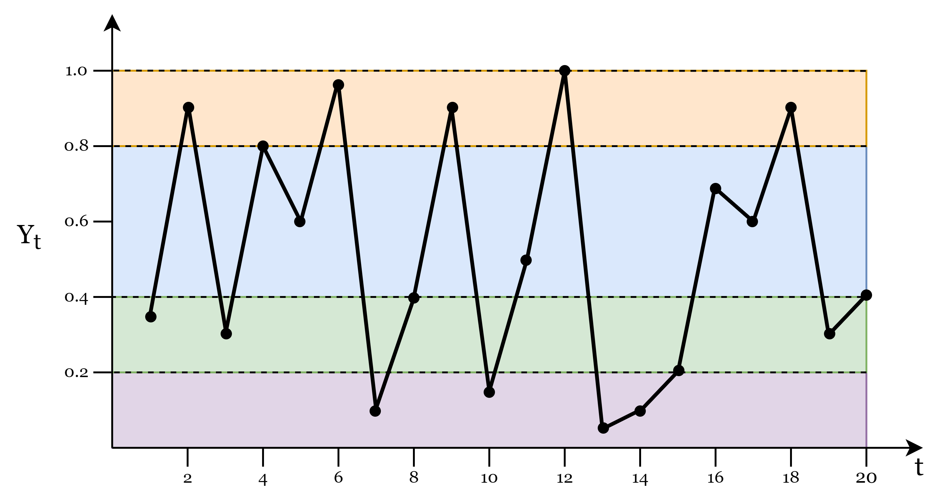
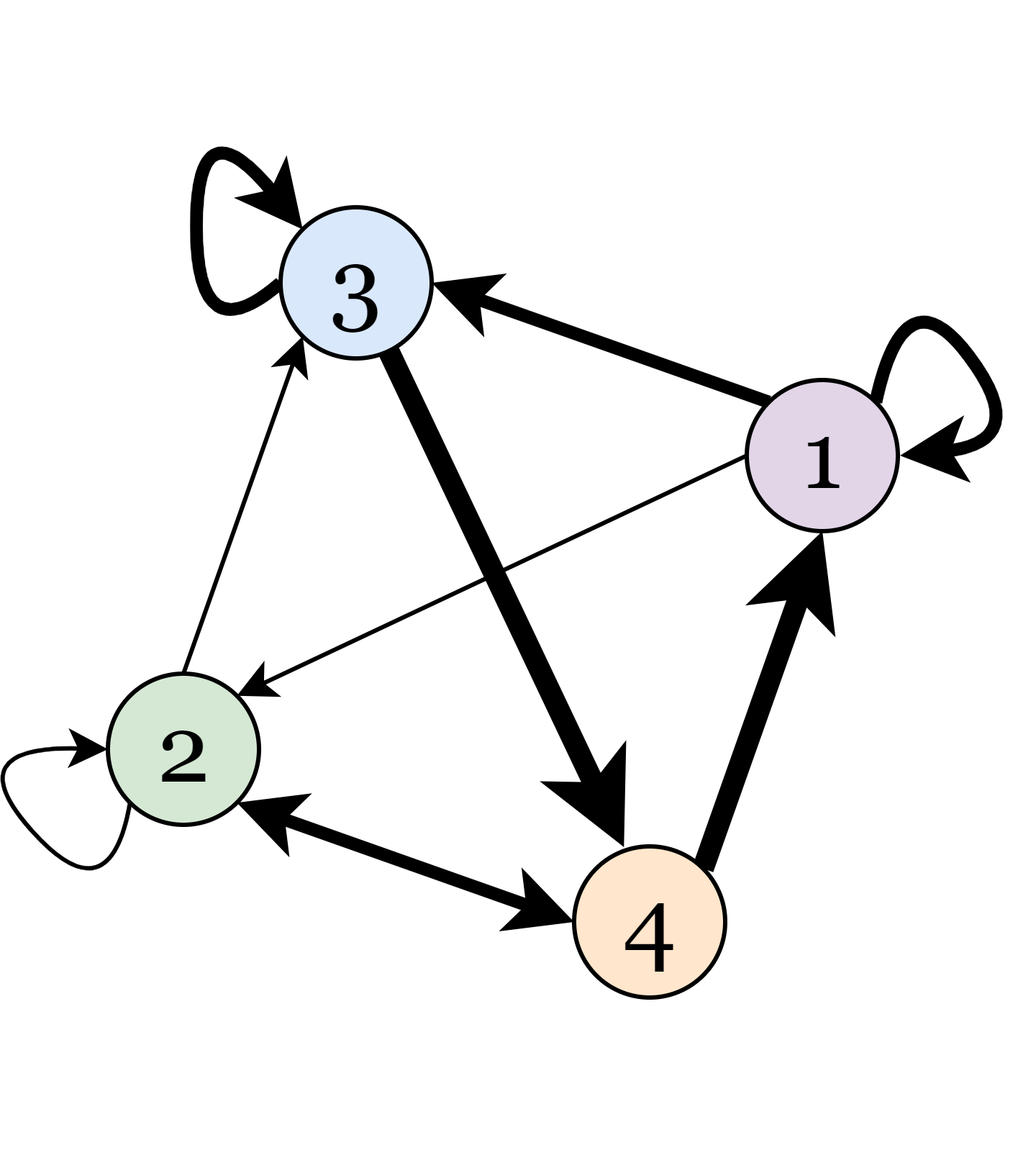
The number of quantiles is usually much less than the length of the time series ($Q\ll T$) and the resulting networks are weighted, directed and contain self-loops. If the number of quantiles is too large the resulting graph may not be connected. On the other hand, QGs present a significant loss of information, represented by large weights assigned to self-loops, when $Q$ is small. Shirazi et al., (2009) proposed a method based on the chi-squared statistic to obtain the optimal number of bins (quantiles). The connectivity of QGs represents the causal relationships contained in the dynamics of the process.

Campanharo and co-authors (Campanharo et al.,, 2011) reconstructed a time series from a QG using only the information contained in the adjacency matrix and without prior knowledge about the original series. These authors have shown that the resulting series presents statistical properties namely, autocorrelation, power spectrum and marginal distributions equivalent to those of the original series.

Recently, Campanharo and Ramos, (2016) developed a variation of the QGs method in order to estimate the Hurst exponent of fractional noise. This variation involves the introduction of a parameter $\phi$ such that two nodes $v_{i}$ and $v_{j}$ are connected by an edge with weight $w_{i,j}^{\phi}$ whenever two observations $Y_{t}$ and $Y_{t+\phi}$ belong to the quantiles $q_{i}$ and $q_{j},$ respectively, where $\phi=1,\ldots\phi_{max}<T$. If $\phi=1$, the method is reduced to QGs. The Hurst exponent, $H$, can be estimated as a function of the mean jump length: $\Delta(\phi)\sim\phi^{H}$, where

$$\Delta(\phi)=\frac{1}{L}\sum_{l=1}^{L}\delta_{l,\phi}(i,j),$$ (18)

$\delta_{l,\phi}(i,j)=|i-j|$, with $i,j=1,\ldots,Q$, is the jumps of length in a random walk on the graph and $L$ is the number of jumps.

Shirazi and co-authors (Shirazi et al.,, 2009) were able to quantify the effect of long range correlations and of the marginal distributions, using distance and clustering measures. They tested the method on synthetic white noise data and on real data from turbulence and stock market index series. Liu and Wang, (2018) also used this approach to identify behavior patterns of the processes underlying synthetic and real world time series data from the visual analysis as well as the analysis of the communities of the resulting networks. Campanharo and co-authors (Campanharo et al.,, 2011) were able to show that time series with different properties are mapped into networks with different topological properties. In particular, as randomness increases in time series, the corresponding QG networks become increasingly random as well, becoming similar to small-world models . Later, Campanharo, (2016) showed that the QGs are capable of capturing and quantifying time series derived from long-range correlated processes and chaotic processes. They also verified that as the time series changes from periodic to chaotic, the corresponding networks, initially regular, become more and more random with larger values of the average path length  and clustering coefficient. The work developed by Campanharo et al., (2018) and Pineda et al., (2020) takes advantage of the quantile graphs to classify EEG data.

3.2.2 Ordinal Partition Transition Networks

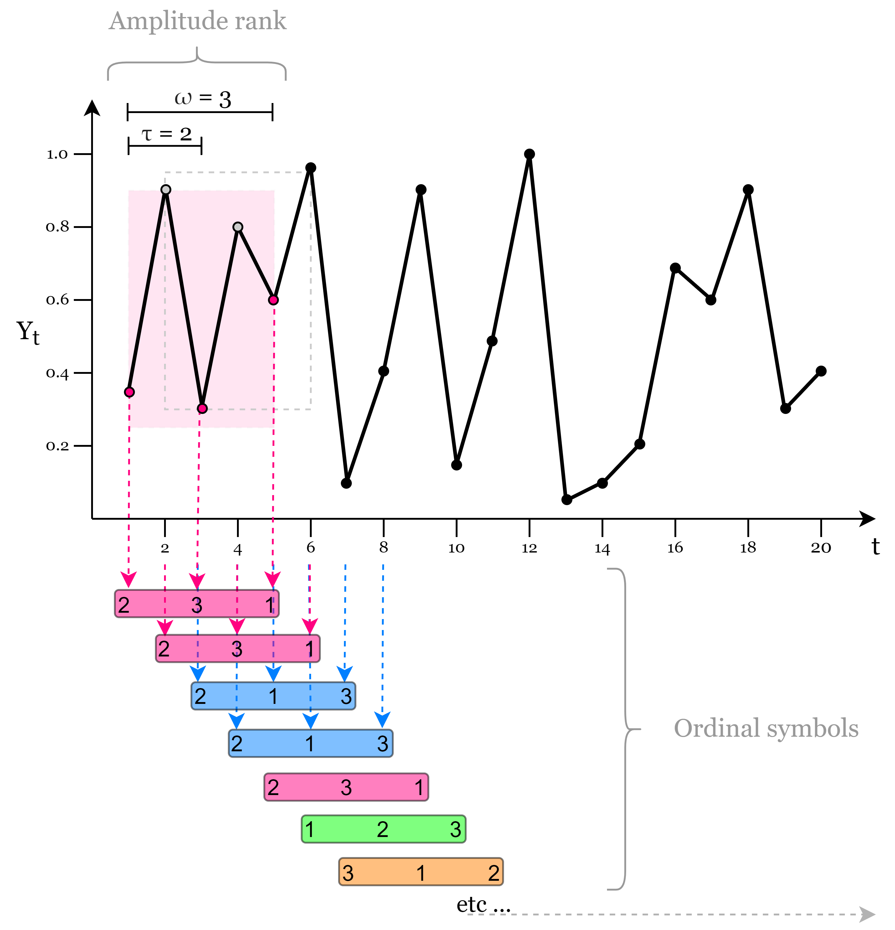
Ordinal patterns methods are based on the idea of a set of sequential patterns defined for a sequence of consecutive observations, where each node of the network represents one of the defined patterns and the edges are weighted according to the transition frequency between two consecutive patterns.

Formally, to construct a network of ordinal patterns (or ordinal partition transition network, OPTN) for a univariate time series the time series is embedded in a $w$-dimensional space using a time delay $\tau.$ For each of these vectors $\vec{z}_{i}$, define the corresponding ordinal pattern by assigning ranks to the data $Y_{t}$ in descending order, $\pi_{i}=(R_{1},R_{2},\ldots,R_{w})$, where $R_{j}\in\{1,2,\ldots,w\},$ $R_{j}\neq R_{k}$ if $j\neq k$. If the observations $Y_{j}$ and $Y_{k}$ for time $j$ and $k$ have equal amplitudes we consider the order of time, we take the first to occur as smallest (Small,, 2013; McCullough et al.,, 2015) (see Figure 9a). Finally, the set of patterns obtained is mapped to nodes in a network where the edges are allocated between nodes based on the transition sequence of the symbols $\pi_{i}$. The weight ($w_{i,j}$) associated with the edge $(v_{i},v_{j})$ is the probability of transition between consecutive symbols.

(a) Toy time series

(b) Ordinal Partition Transition Network

Figure 9: Illustrative example of ordinal partition transition network algorithm. On the left side we illustrate the method of embedding with window size $w=3$ and lag $\tau=2$ and the method of find its ordinal pattern, based in the amplitude rank of its elements. On the right side we show the resulting networks.

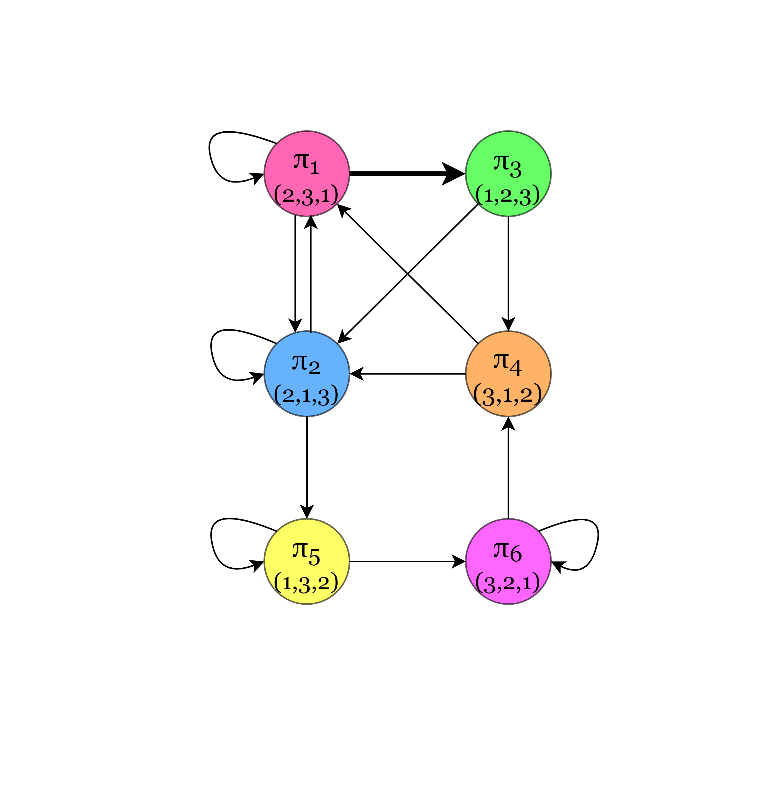
McCullough and co-authors (McCullough et al.,, 2015), applied the ordinal partitions method to the R$\ddot{\text{o}}$ssler system and to other chaotic series. They found that both the visual topological structure of the networks, time series with periodic behavior are mapped in networks with a ring structure and chaotic time series in networks with band or tube-like structures, and the simple topological metrics as average out-degree and variance of out-degrees, convey the dynamics underlying the processes. In particular, the average out-degree and the variance of out-degrees allow to detect changes in the dynamic behavior in a similar way to the Lyapunov exponent , distinguishing dynamics of different states and determining points of change. These networks also proved to be useful for the analysis of real world time series, such as: series from the externally driven diode resonator circuit (McCullough et al.,, 2015), and electrocardiograms (ECG) series for analysis of dynamical changes, as human cardiac dynamics (Cao et al.,, 2004; McCullough et al.,, 2017).

A number of studies have begun to emerge around the so-called forbidden patterns, which are patterns that do not occur in a time series. These studies have shown that measures around these patterns, namely the counting of forbidden patterns, are important to distinguish deterministic time series with very high levels of noise from random series (Amigó et al.,, 2007), to detect of determinism in noisy data (McCullough et al.,, 2016; Sakellariou et al.,, 2016), and to distinguish between healthy patients and unhealthy patients with varying heart conditions based in ECG data (Kulp et al.,, 2016).

Recently, Pessa and Ribeiro, (2019) showed that properties of ordinal networks (namely, the average weighted shortest path lengths) can be used for estimating the Hurst exponent of time series with high precision, outperforming the quantile graphs (Campanharo and Ramos,, 2016) and the detrended fluctuations analysis (Shao et al.,, 2012).

3.2.3 Coarse-Grained Phase Space Graphs

Networks based on coarse-graining of phase space consist of the idea of reconstructing (creating sets of symbol groups) the phase space of a dynamic process, where each of these symbol groups are mapped into a node of network and the edges are established between nodes representing successive partitions in time. A weight representing the amount or probability of transition between these partitions (nodes) is assigned to the edge.

The algorithm involves the following steps (Gao and Jin,, 2009; Wang and Tian,, 2016): start by embedding a time series in a $w$-dimensional space with a time delay $\tau$, similarly to ordinal partition transition networks (Subsection 3.2.2); then the vectors (points in the phase space) $\vec{z}_{t}=(Y_{t},Y_{t+\tau},\ldots,Y_{t+(w-1)\tau})$ are classified into $D=w$ different symbol groups ($\Psi_{j}=\{\psi_{i}\}_{i=1}^{D}$), according to intervals predefined by a set of values that delimit the phase space $\{\alpha_{1},\ldots,\alpha_{D-1}\}$ (Wang and Tian,, 2016; Zou et al.,, 2019):

$$\left\{\begin{array}[]{l}\psi_{1}\quad\textrm{if }Y_{t}<\alpha_{1},\\ \psi_{i}\quad\textrm{if }\alpha_{i-1}\leq Y_{t}<\alpha_{i},\ 1<i<D-1\\ \psi_{D}\quad\textrm{if }Y_{t}\geq\alpha_{D-1}.\\ \end{array}\right.$$ (19)

Note that this transformation process is similar to the transformation underlying the QG algorithm (Subsection 3.2.1), but applied separately to each component of the embedding vector. While in QGs, quantiles delimit the time series support, here the set of values $\{\alpha_{1},\ldots,\alpha_{D-1}\}$ delimit the phase space. Finally, each unique vector of symbols $\Psi_{j}$ is mapped into a node of network. Directed and weighted edges $(v_{i},v_{j},w_{i,j})$ are defined by the transition probabilities between symbol vectors $\Psi_{i}$ and $\Psi_{j}.$

Wang and Tian, (2016) have shown, based on the distribution of weighted degree of nodes, that increasing the dimension $w$ of the phase space leads to enhancing the heterogeneity of the networks and that the method allows distinguishing and characterizing different series, such as white noise, chaotic Lorenz systems, and gasoline price series.

Weng and co-authors (Weng et al.,, 2017) proposed an extension of this algorithm with the purpose of characterizing the memory (short or long) of the process. Taking into account that the temporal information is lost after the coarse-graining transformation and that the transition probability matrix is an estimate of the process dynamics, Weng and co-authors proposed to incorporate the temporal information into an additional topological dimension, such as an edge attribute. In this network, a node $v_{i}$ is connected to the node $v_{j}$ with an attribute $t,$ $(v_{i},v_{j};t)$, when a transition from $\Psi_{i}$ to $\Psi_{j}$ occurs at time stamp $t$. This makes it possible to construct a memory network whose memory effect appears to be able to accurately differentiate various types of time series, namely, white noise, 1/f noise, AR model, periodic and chaotic time series.

3.2.4 Visibility Graphlets Networks

Given the ability to incorporate the topological characteristics (global and local) of the time series in the visibility graphs, visibility graphlets networks were proposed by Mutua et al., (2015) in order to monitor and, consequently, understand the evolutionary behaviors of a time series. The method consists of five fundamental steps (Mutua et al.,, 2015, 2016). First, a time series is incorporated into a $w$-dimensional space without time delay ($\tau=1$), similarly to sliding a window of length $w$ across the time series; each resulting vector $\vec{z}_{k}=(Y_{k},Y_{k+1},\ldots,Y_{k+w-1}),$ with $k=1,2,\ldots,T-w+1,$ is mapped to a directed visibility graph (visibility graphlet) $G_{k},$ following the algorithms described in Subsections 3.1.1 and 3.1.3, representing the $k$-th sate of the time series; the successive visibility graphs are then connected by a directed edge resulting in the following state chain network: $G_{1}\to G_{2}\to\ldots\to G_{T-w+1}.$ In order to obtain a network of distinguishable states, each graph $G_{k}$ is, iteratively, compared to the others across the chain network and if any two graphs are identical, i.e., the adjacency matrices are the same, the latter graph is replaced by the former which is the reference state. For example, if $\boldsymbol{A}_{1}=\boldsymbol{A}_{5},$ the graph (state) $G_{5}$ is replaced by $G_{1}.$ Finally, the visibility graphlets network is defined so that the nodes represent the unique graphlets and the directed and weighted edges are established between pairs of nodes with weight equal to the number of edges between the successive corresponding graphlets in the chain network.

Visibility graphlets network is a directed and weighted transition network where the time series states are represented by visibility graphlets and the edges reflect the relative frequency of states sequences, i.e., the transfer behaviors of the unique states. This network can also be seen as a temporal network (Holme and Saramäki,, 2012) and a network of networks (Kivelä et al.,, 2014), where the corresponding network science methodologies can be used (Mutua et al.,, 2015). This mapping method is a ”mixture” of two underlying concepts, visibility and transition probability, which can benefit from the characteristics mapped by both, namely, structural features that fully describe the states of the time series and the dynamic transfers of the underlying processes. However, like all methods that involve incorporation in the phase space, the selection of the parameter $w$ is a problem. If $w$ is too small, the number of different graphlets is very limited. On the other hand, the number of different graphlets increases geometrically with the increase of $w$ implying that the time series is sufficiently large. See Mutua et al., (2015) for a more detailed discussion.

In Mutua et al., (2015), the authors studied some properties in a set of synthetic and real world time series, namely, degree of nodes and transmission probability related to edge weights for short-term prediction, and long-term persistence related to the occurring positions of some motifs on time series. Mutua et al., (2016) used the method in discrete and continuous chaotic time series and showed that the generated networks capture the dynamic properties of the systems, distinguishing chaotic zones that result in networks with a complex structure characterized by hubs and non-chaotic zones, such as periodic ones that result in regular networks.

3.3 Proximity Networks

Mappings based on the concept of proximity use measures of distance or similarity to calculate the distance between the points of the time series incorporated in the multidimensional phase space. These methods map states of the time series into nodes of the network and create edges between those nodes based on some measure of distance or similarity. The ability to connect different nodes based on proximity measures allows capturing significant information about the topology of the dynamical systems, enabling to identify, for example, different regimes or patterns along the series via the similarity of successive states (Donner et al., 2011b, ).

Proximity networks include cycle networks, correlation networks, and recurrence networks.

3.3.1 Cycle Networks

Cycle networks were proposed by Zhang and co-authors (Zhang et al.,, 2006; Zhang and Small,, 2006) to represent pseudo-periodic time series.

Formally, to construct a cycle network from a pseudo-periodic time series $\{Y_{t}\}_{t=1}^{T},$ first segment the series into $u$ consecutive cycles $\{c_{1},c_{2},\ldots,c_{u}\}$, not necessarily of the same length, according to the local minima (or maxima). For each pair of cycles $c_{i}=\{Y_{i},\ldots,Y_{l_{i}}\}$ and $c_{j}=\{Y_{j},\ldots,Y_{l_{j}}\}$ ($i,j=1,2,\ldots,u$ and $i\neq j$) compute the correlation index $r_{i,j}$ defined as the maximum of the cross-correlation between the two cycles (assuming that $l_{i}\leq l_{j}$ without loss of generality) (Zhang et al.,, 2006):

$$r_{i,j}=\underset{l=0,1,\ldots,l_{j}-l_{i}}{\max}\frac{\mbox{\rm cov}[(Y_{i},\ldots,Y_{l_{i}}),(Y_{1+l},\ldots,Y_{l_{j}+l})]}{\sqrt{\mbox{\rm var}(Y_{i},\ldots,Y_{l_{i}})}\sqrt{\mbox{\rm var}(Y_{1+l},\ldots,Y_{l_{j}+l})}},$$ (20)

where cov is the covariance and var is the variance. This means that, if the cycles are not of the same length, the shortest, $c_{i}$ is shifted relative to the longest, $c_{j}$ by $l_{j}-l_{i}$ steps and the correlation coefficient between $c_{i}$ and the corresponding part of $c_{j},$ in each step, is calculated. Finally, the highest value is chosen as the correlation coefficient between $c_{i}$ and $c_{j}$. The graph $G$ is constructed by assigning a node $v_{i}$ to each cycle $c_{i}$ and defining an undirected and unweighted edge between two nodes $v_{i}$ and $v_{j}$ if the correlation index is above a certain threshold $r_{i,j}>\alpha.$

The definition of the edges may be alternatively based on other distance measures, such as

$$d_{i,j}=\underset{l=0,1,\ldots,l_{j}-l_{i}}{\min}\frac{1}{l_{i}}\sum_{k=1}^{l_{i}}\|Z_{k}-X_{k+l}\|,$$ (21)

for which thresholds must also be set (Zhang and Small,, 2006).

Zhang and Small (Zhang and Small,, 2006) applied cycle networks to the study of the R$\ddot{\text{o}}$ssler system and of electrocardiogram (ECG) signals. The authors studied topological metrics of the resulting graphs, such as degree distribution, among others, and concluded that noisy periodic signals are mapped into random networks and chaotic time series into networks that exhibit small-world and scale-free features. In particular, they observed peaks in the degree distribution function of the graph that correspond to the unstable periodic orbits of the system, the nodes corresponding to these orbits form communities in the network. The metrics studied also allowed to distinguish between ECG of healthy volunteers, $P(k)$ varies smoothly, and those of unhealthy patients, $P(k)$ shows more prominent variations.

3.3.2 Correlation Networks

Correlation networks are essentially constructed based on a correlation measure, such as the correlation matrix of the time series $Y_{t}$ proposed by Yang and Yang, (2008) based on the ideas of functional networks (Eguiluz et al.,, 2005), correlation of stock markets (Bonanno et al.,, 2004) and the results obtained by cycle networks (Zhang and Small,, 2006). The process consists of first considering individual state vectors $\vec{z}_{i}$ of time series which are extracted by embedding the series into a sufficiently large $w$-dimensional space. Each state vector is mapped into a node $v_{i}$ of an undirected and weighted network where the set of edges $\{(v_{i},v_{j},w_{i,j})\}$ are established in terms of the Pearson correlation coefficient calculated between the corresponding state vectors $(\langle\vec{z}_{i},\vec{z}_{j}\rangle).$ Note that the Pearson correlation takes values between $-1$ and $1$, and so a negative weight may be assigned to the edges. However, as already mentioned, network analysis with negative weights is unusual and so the weights of correlation networks are usually established as the absolute value of the correlations, $w_{i,j}=|\rho_{i,j}|.$ The correlation matrix $[|\rho_{i,j}|]$ is the matrix of the correlation network, and note that other measures of correlation may be considered.

As with cycle networks, a threshold $r_{c}$ also can be considered and a binary adjacency matrix can be produced. This threshold must be chosen properly because it determines the characteristics of the resulting network. If it is extremely small, pairs with weak correlations are also connected (noise). But if it is too large important information may be lost too (Yang and Yang,, 2008).

Correlation networks were applied to stock price series (return and amplitude series) resulting in a degree distribution function that follows a perfect Gaussian distribution. Additionally, the return series point to a random behavior, indicating that the global correlation characteristic can be modeled by an Erdős-Rényi network (Yang and Yang,, 2008). The authors used the degree distribution to decide the best parameters for the algorithm. In contrast, Feng and He (Feng and He,, 2017), used the cross-correlation as a measure of similarity between two points in phase space, and used the clustering coefficient and efficiency to decide the best parameters for the model. They analyzed the Lorenz system, white Gaussian noise and sea clutter time series. The results show that, for an unknown complex system, dynamic states, i.e., the behavior changes of the system, can be discovered by studying the community structures of complex networks. In particular, Feng and He identified changes in behavior from the contractive state to the open state in the sea clutter time series and for the white Gaussian noise did not identify clear community structures, the behavior changes of white Gaussian noise are completely random and therefore the resulting networks do not present a topology in communities.

3.3.3 Recurrence Networks

Recurrence networks are quite popular in the research community. These networks are based on recurrence plots, a tool used in the study of dynamical (non-linear or chaotic) systems (Marwan,, 2008). For constructing a recurrence plot for a dynamical system from an observed time series, first embed the time series in a $w$-dimensional space (phase space reconstruction) thus defining a set of vectors $\vec{z}_{i}.$ Then define a matrix $\boldsymbol{A}$, also called the recurrence matrix, where the elements $(i,j)$ are defined based on the proximity relation in phase space of the vectors $\vec{z}_{i}$ and $\vec{z}_{j}$ (Eckmann et al.,, 1987). The proximity relation can be defined by different criteria, namely, fixed (probability) mass, where a fixed amount of nearest neighbor vectors is established, or fixed volume, where an $\varepsilon$-threshold of proximity is established. The matrix $\boldsymbol{A}$ is commonly defined with elements:

$$A_{i,j}=\left\{\begin{array}[]{l}1\quad\textrm{if }\|\vec{z}_{i}-\vec{z}_{j}\|\leq\varepsilon\\ 0\quad\textrm{otherwise}\\ \end{array}\right.,$$ (22)

where $\varepsilon$ is a distance threshold and $\|\cdot\|$ can be any norm in phase space (for example, Euclidean, Manhattan, or maximum norm) (Marwan et al.,, 2007). The matrix $\boldsymbol{A}$ is a symmetric ($A_{i,j}=A_{j,i}$) matrix with constant values on the diagonal ($A_{i,i}=1$), and it can be interpreted as the adjacency matrix of an undirected and unweighted network, the recurrence network, where the nodes represent $\{\vec{z}_{i}\}$ and the edges are defined by $A_{i,j}$, usually the self-loops are removed ($A_{i,i}=0$). A direct generalization is considering the associated distance matrix between pairs of states, resulting in a weighted network. This type of networks, both weighted and unweighted, are spatial networks, where the nodes (states) are located in an $m$-dimensional space equipped with a norm in the phase space and which is reflected in the topological characteristics/features of the networks (Donner et al.,, 2010). In the unweighted networks case, the probability of finding an edge between two states will decrease with the distance. For weighted networks, the direct use of the distance matrix is generally avoided because the more distant/dissimilar two states are, the stronger the connection between them. To avoid this other alternatives can be used, such as, the inverse of the distance $w_{i,j}=\frac{1}{\|\vec{z}_{i}-\vec{z}_{j}\|}$ (Strozzi et al.,, 2011). Recently, a general alternative, that can be applied to any kind of network, was presented to recurrence networks where weights are given by: $w_{i,j}=\frac{\sqrt{k_{i}k_{j}}}{k_{max}},$ $k_{max}$ is the maximum degree in the unweighted recurrence network (Jacob et al.,, 2019).

The construction of these networks implies that they do not incorporate any temporal information on the underlying process and therefore do not explicitly depend on the presence of equally spaced observations, which is a major issue in the analysis of time series observed in many phenomena (Donner et al., 2011b, ). Recurrence plots are also one of the few time series analysis techniques that work well with non-stationary time series data. However, in the case of more complex systems, the rich geometric structure of recurrence plots can become difficult to interpret, for example, for chaotic systems this happens due to their unstable periodic orbits (Bradley and Kantz,, 2015). The characteristics and topological properties of recurrence networks depend essentially on their construction, namely on the following parameters: dimension of states $w$, time delay $\tau$ and threshold $\varepsilon$, the measure of proximity between states. It is important to note $w=1$ meaning that the embedding in the phase space is not required in which case the distance is computed between the points of time series (Marwan et al.,, 2009; Zhao et al.,, 2020).

The literature essentially highlights three types of recurrence networks, the $\kappa$-nearest neighbor networks, the adaptive nearest neighbor network and the $\varepsilon$-recurrence networks, which we describe in more detail below.

$\kappa$-Nearest Neighbor Networks, $\kappa$-NNN

The $\kappa$-nearest neighbor version imposes a constraint on the quantity $\kappa$ of the nearest neighbor points (nodes $v_{j}$) of a given point in the phase space (node $v_{i}$). This implies a direction in the edge $(v_{i},v_{j})$ since it is not necessarily true that, if the node $v_{j}$ is one of the $\kappa$ the closest neighbors of the node $v_{i}$ then $v_{i}$ is also one of the $\kappa$ closest neighbors to $v_{j}$, and so the adjacency matrix becomes an asymmetric matrix. This method was proposed by Small and co-authors (Small et al.,, 2009), in order to overcome the issue of cycle networks mappings that requires time series with an oscillatory nature.

$\kappa$-NNN imply that all nodes have the same amount $\kappa$ of out-edges, $k_{i}^{out}=\kappa$, preserving a constant mass of the considered neighborhoods, i.e., the number of nodes is the same in all neighborhoods (Donner et al., 2011b, ). However, the distribution of in-edges $k_{i}^{in}$ is allowed to vary but the average degree is $\bar{k}^{in}=\kappa$. In particular, if $k_{i}^{in}\ll\kappa$, the node $v_{i}$ must be in a phase space region with decreased density compared to the remaining, and if $k_{i}^{in}\gg\kappa$, $v_{i}$ must be located in a densely populated region (Donner et al., 2011b, ), thus giving information about the local geometry of the phase space.

Xiang et al., (2012) studied the distribution of network motifs in $\kappa$-NNN and were able to classify different dynamic behaviors (such as maps and flows) using the frequency of motifs. These authors have also shown that degree variations accompany the changes in the dynamics throughout the bifurcation process of the R$\ddot{\text{o}}$ssler system.

Adaptive Nearest Neighbor Networks, ANNN

In order to overcome the imposition that all nodes have the same $k_{i}^{out}=\kappa$ in $\kappa$-nearest neighbor networks, a new version, called adaptive nearest neighbor networks, was proposed (Xu et al.,, 2008; Small et al.,, 2009). In ANNN if $v_{j}$ is one of the $\kappa$ closest neighbors of $v_{i},$ then $v_{i}$ is also considered a neighbor of $v_{j},$ even if it is not one of the $\kappa$ closest neighbors to $v_{j}.$ This leads to a symmetric adjacency matrix and the node degree to be variable, unlike $\kappa$-NNN, since there may be more than $\kappa$ neighbors to a given node. Xu et al., (2008) and Liu and Zhou, (2010) have shown that the motif distributions allow characterizing different processes, namely periodic, chaotic, noise and fractional, creating super-families. Unique fingerprints have also been found for specific dynamical systems within a family. Additionally, Liu and Zhou, (2010) analyzed three stock market indexes and concluded that the motif distributions are equivalent for the three series (since they have the same dynamic behavior characteristic of return stock series) and are also very similar to the distributions obtained for the fractional Brownian motion .

$\varepsilon$-Recurrence Networks

Equation (22) suggests that the ”neighborhood” of a single state vector $\vec{z}_{i}$ can be defined by a fixed distance in the phase space $\varepsilon$, considering fixed volumes (communities) in phase space (Donner et al., 2011b, ). Thus, an undirected and unweighted network can be built.

This version implies choosing the distance threshold $\varepsilon$ which allows to control the phase space resolution. If $\varepsilon$ is too small, the volume of the neighborhood will be small and therefore there will be almost no recurrence points and the information incorporated in the network will be insufficient. On the other hand, if $\varepsilon$ is too large we observe a general qualitative change in the network topology (Jacob et al.,, 2016), namely, each node will behave like a hub, leading to an excess of recurring points and misleading information.

Donner and co-authors (Donner et al.,, 2010; Donner et al., 2011b, ) studied properties of $\varepsilon$-recurrence networks at three different scales, namely local, intermediate and global on several paradigmatic systems: Hénon map, Bernoulli map, Lorenz system and R$\ddot{\text{o}}$ssler system. The authors studied graph properties as a function of the distance threshold $\varepsilon$ and proposed specific measures like the local clustering coefficient to detect dynamically invariant objects, saddle points or unstable periodic orbits. Moreover, those authors suggested varying the embedding dimension as a means to distinguish between chaotic and stochastic systems. Zou et al., (2012) have shown that the degree distribution of networks generated for one-dimensional maps with a local power-law in the invariant density is a scale-free distribution, resulting in scale-free networks. In a general case, the resulting exponent of the degree distribution does not need to coincide with the fractal dimension. In this direction, Donner et al., 2011a demonstrated that the local and global transitivity of the networks are closely related with a generalized notion of fractal dimensionality (local and global, respectively).

$\varepsilon$-recurrence networks were the most exploited and led to the well-established relationships between some topological metrics of networks and the properties and measurements of phase space. Donges and co-authors (Donges et al.,, 2012) propose an analytical framework for $\varepsilon$-recurrence network analysis describing graph-theoretical recurrence network quantifiers. This framework shows that several standard measures of network analysis can represent discrete estimators of continuous measures of certain complex phase space properties. A theoretical relation is established between measures of the recurrence networks and phase space properties. $\varepsilon$-recurrence networks were also widely used to determine changes in the dynamics of theoretical (Marwan et al.,, 2009; Iwayama et al.,, 2013) and real world (Donges et al., 2011a, ; Fukino et al.,, 2016) systems.

4 Mapping Multivariate Time Series into Complex Networks

So far we have focused on approaches to mapping univariate time series into network structures. However, technological developments are producing a wealth of inter-linked multidimensional data, such as multivariate spatio-temporal data. Tools for the analysis of these high dimensional data sets are yet scarce, hinting at the possibility of using network science approaches. The literature on mapping multivariate time series to the network domain, summarized in Table 2, is not as developed as for the univariate case. Even so, we can distinguish two classes of methods, introduced in Figure 1: those that map the multivariate time series into a single layer or monoplex network and those that map the multivariate time series into a multiplex network. The mappings in the first class construct networks with nodes representing the (component) time series and edges representing the relationship between the node time series, computed as, e.g., causal relation. Mappings on the second class lead to multiplex networks where each layer is a network resulting from a univariate time series mapping. The layers usually have the same nodes and are connected via the edges which connect the same node across adjacent layers. Details on each approach and corresponding core results are given in the following sections.

		Network Type (original reference)	Node	Edge	Directed	Weighted	Param-free	Pre pross
Single	Layer	Correlation Network	$Y_{\alpha,t}$	CM	✗	✓	✓	✗
		(Eguiluz et al.,, 2005)
		Long-Run Variance Decomposition Network	$Y_{\alpha,t}$	VD	✓	✓	✗	VAR
		(Diebold and Yılmaz,, 2014)
		Causal Effect Network	$t$	LCR	✓	✓	✗	CDA
		(Runge et al.,, 2015)
		Ordinal Partition Transition Network	$\pi_{i}$	TP	✓	✓	✗	PS
		(Zhang et al., 2017a, ; Ruan et al.,, 2019)
		Pattern Interdependent Network	$G_{i}$	TP	✓	✓	✓	PS;VG
		(Ren et al.,, 2020)
		Inter-system recurrence network	$\vec{z}_{i}^{[\alpha]}$	DM	✗	✗	✗	PS
		(Feldhoff et al.,, 2012)
		Joint Recurrence Network	$\vec{z}_{i}^{[\alpha]}$	DM	✗	✗	✗	PS
		(Feldhoff et al.,, 2013)
Multiple	Layer	Multiplex Visibility Network	$t$	V	✗	✗	✓	✗
		(Lacasa et al.,, 2015)
		Multiplex Recurrence Network	$t$	DM	✗	✗	✗	PS
		(Eroglu et al.,, 2018)

Table 2: Comparison of (multivariate) time series mappings based on the properties of the corresponding algorithms and of the resulting networks. Notation: CM - correlation measures, VD - variance decomposition, LCR - lagged causal regression, TP - transition probability, DM - distance measures, V - natural and/or horizontal visibility, VAR - vector autoregression model, CDA - causal discovery algorithm, PS - phase space, VG - directed visibility graph.

4.1 Correlation Networks

Formally, a correlation network (CN) is defined as an undirected and weighed graph $G=(V(G),E(G))$ where $V(G)=\{Y_{i,t}\}_{i=1}^{m}$ and $E(G)=\{(v_{i},v_{j},w_{i,j})|(v_{i},v_{j})\in V(G)\wedge w_{i,j}=\rho_{i,j}(0)\wedge i\neq j\}$ (see in 2.1). Thus, inter-dependencies between the $m$ time series are represented by the (contemporaneous) correlation.

Other approaches to represent the inter-dependencies and establish the edges of the network rely on suitable correlation measures such as cross-correlations (Nakamura et al.,, 2016) or partial correlations (Epskamp and Fried,, 2018), eventually subject to thresholding. The thresholding (edges are established only if the correlation exceeds a predefined value) helps to remove spurious edges. Alternatively, correlations can be replaced by any similarity measure, including distance measures. The resulting similarity/distance matrix is then used to construct a monoplex network (Mori et al.,, 2016).

Figure 10 presents an example of a correlation network representation of a toy multivariate time series. Nodes that represent similar time series are linked by thicker edges.

(a) Toy time series

(b) CN

Figure 10: Illustrative example of the correlation network algorithm. On the left side we present the plot of a toy multivariate time series and on the right side the network generated by the correlation algorithm (using contemporaneous cross-correlation). The different colors represent the time series. Higher correlation values result in edges in the network with larger weights represented by thicker lines.

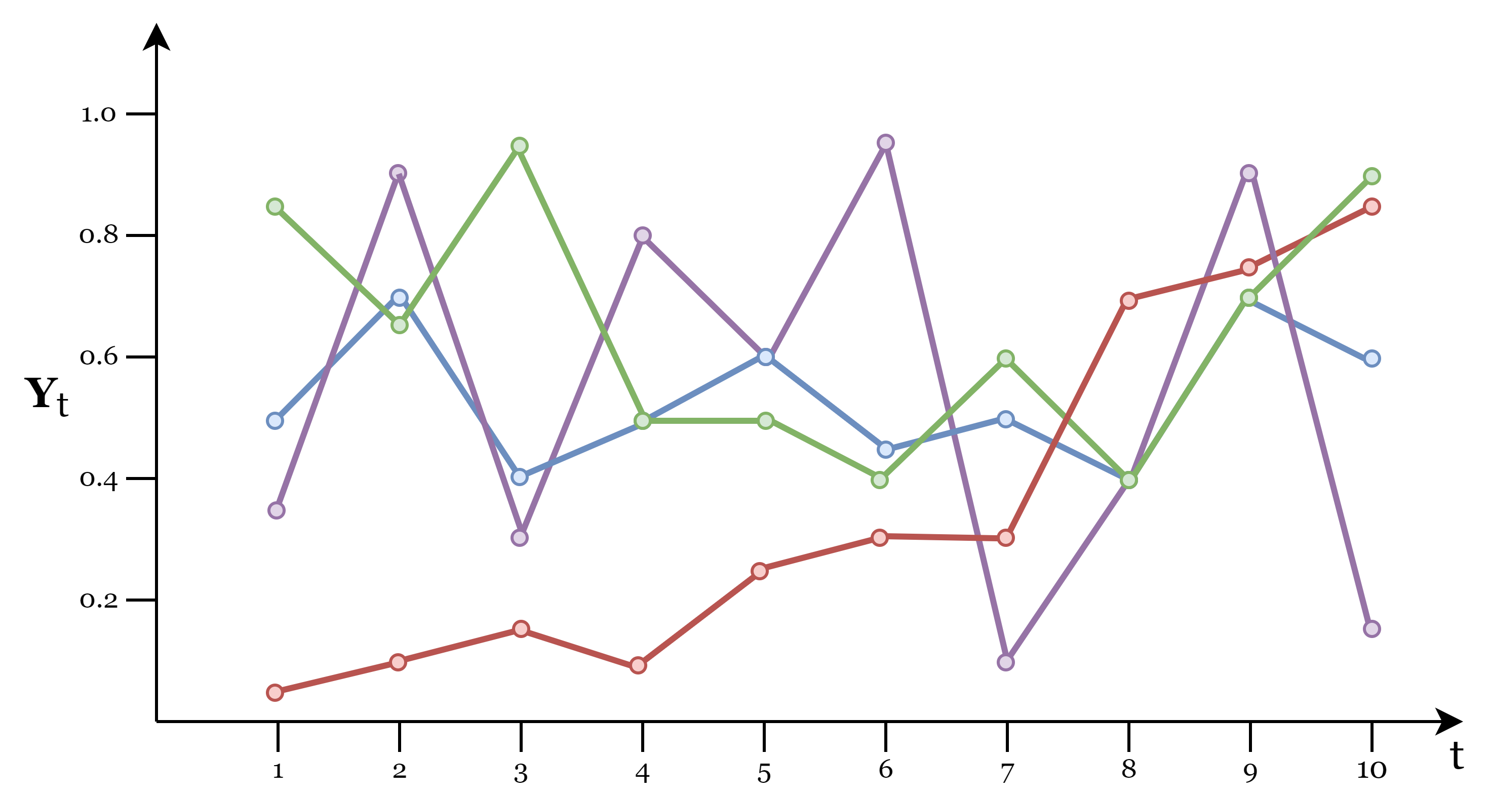
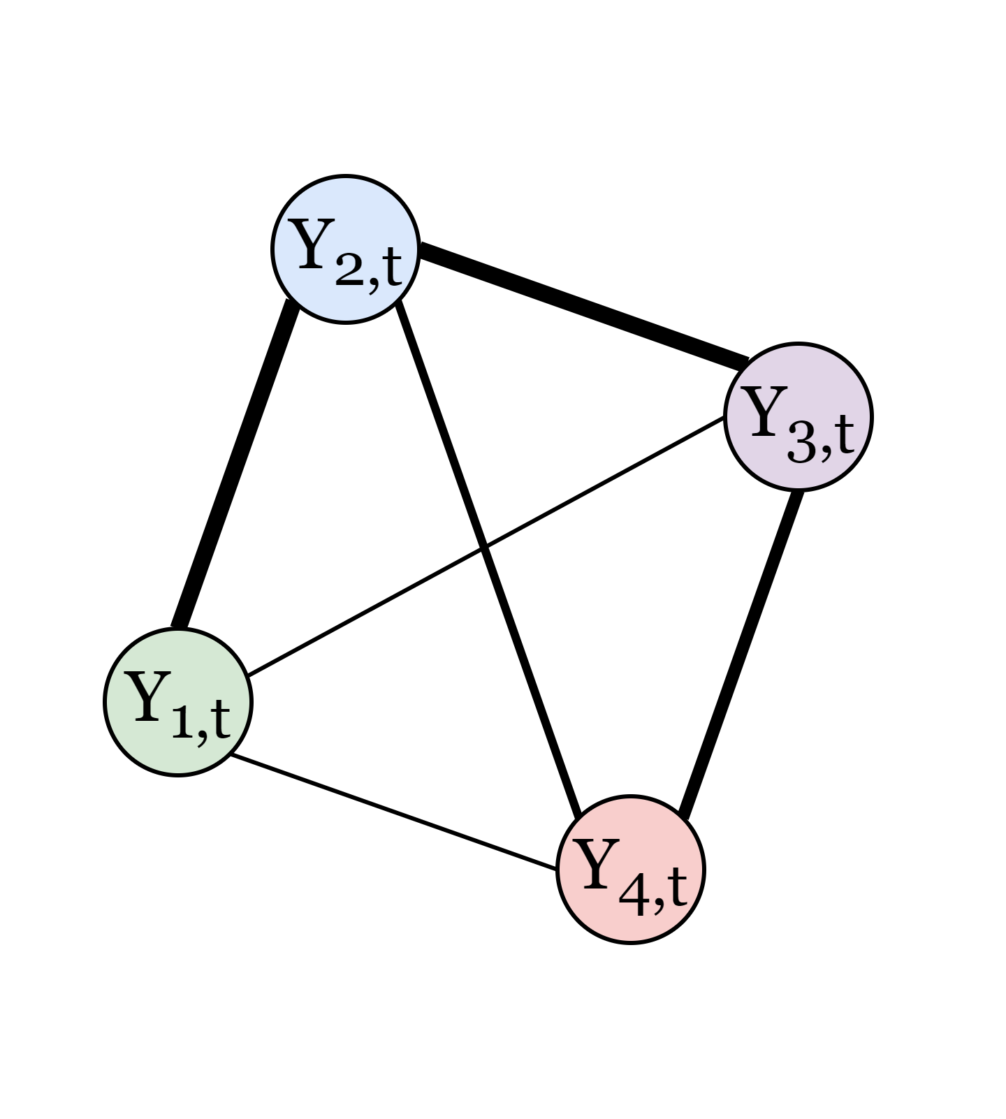
Correlation networks (also known as functional networks) have been widely used in neuroscience (Eguiluz et al.,, 2005; Bullmore and Sporns,, 2009), financial (Tumminello et al.,, 2010; Cai et al.,, 2010; Gao et al.,, 2015) and climate science (Tsonis and Swanson,, 2012; Dijkstra et al.,, 2019) areas. In particular, Eguiluz and co-authors (Eguiluz et al.,, 2005) applied this approach to functional fMRI data in order to connect brain zones based on their similarities and their relationships. They have shown that the degree distribution obeys a power law, indicating scale-free networks which implies that there are always a few zones of the brain (hubs) with relations to most other regions of the brain, that is, predominant zones.

Gao and co-authors (Gao et al.,, 2015) used correlation networks to analyze the interactions between companies of the different sectors using clustering metrics. The objective is also to study the influence that some companies and/or sectors have on others. The results show important information about fluctuations of the series and show that correlation networks can be very useful for financial risk analysis.

4.2 Long-Run Variance Decomposition Networks

The mapping of multivariate time series into correlation networks is based on the contemporary dependence of time series, but in multivariate time series, cross-sectional dependencies may arise in different leads/lags (Lanne and Nyberg,, 2016). We introduce now a class of networks that reflect, in the directed and weighted edges, the presence of contemporaneous as well as lagged partial correlations between time series $Y_{i,t}$ and $Y_{j,t}$. The edges of the network are established via Vector AutoRegression (VAR) models and their analysis, namely Forecast Error Variance Decomposition (FEVD). The process $\boldsymbol{Y}_{t}$ follows a VAR($p$) model, where $p$ is the order of the VAR, if it satisfies the following equation:

$$\boldsymbol{Y}_{t}=c_{0}+\sum_{i=1}^{p}\boldsymbol{\Phi}_{i}\boldsymbol{Y}_{t-i}+\boldsymbol{a}_{t},$$ (23)

where $c_{0}$ is an $m$-vector of constants, $\boldsymbol{\Phi}_{i}$ $(i=1,2,\ldots,p)$ is an $m\times m$-matrix of coefficients to be estimated and $\boldsymbol{a}_{t}$ is an $m$-vector of uncorrelated errors with zero mean and covariance matrix $\boldsymbol{\Sigma},$ with elements $\sigma_{i,j}$. Under stationarity conditions $\boldsymbol{Y}_{t}$ may be represented as an infinite moving-average representation (MA model)

$$\boldsymbol{Y}_{t}=\sum_{j=0}^{\infty}\boldsymbol{\Theta}_{j}\boldsymbol{a}_{t-j}.$$ (24)

The FEVD, carried out typically on the infinite moving-average representation of the VAR process, calculates the proportion of the prediction error variance of the $i$-th variable which is assignable to its own (lagged) shocks and to the (lagged) shocks of the other variables. A problem with the FEVD is that it is dependent of the ordering of the variables. To overcome this issue, Diebold and Yılmaz, (2014) and Lanne and Nyberg, (2016) propose to use the generalized forecast error variance decomposition (GFEVD) which is independent of the ordering of the variables. Thus, a long-run variance decomposition network (LVDN) is a network where the nodes $v_{i}$ and $v_{j}$ represent the time series $Y_{i,t}$ and $Y_{j,t},$ respectively, and the edges $(v_{i},v_{j},w_{i,j})$ are given by $w_{i,j}=\frac{d_{i,j}^{h}}{\sum_{j=1}^{T}d_{i,j}^{h}}$, where $d_{i,j}^{h},$ denotes the $(i,j)$-th $h$-step ahead variance decomposition component, that is, the fraction of variable $i$ $h$-step ahead forecast error variance due to shocks in variable $j$ (Diebold and Yılmaz,, 2014), calculated as:

$$d_{i,j}^{h}=\frac{\sigma_{j,j}^{-1}\sum_{k=0}^{h-1}(\boldsymbol{\epsilon}_{i}^{{}^{\prime}}\boldsymbol{\Theta}_{k}\boldsymbol{\Sigma}\boldsymbol{\epsilon}_{j})^{2}}{\sum_{k=0}^{h-1}(\boldsymbol{\epsilon}_{i}^{{}^{\prime}}\boldsymbol{\Theta}_{k}\boldsymbol{\Sigma}\boldsymbol{\Theta}_{k}^{{}^{\prime}}\boldsymbol{\epsilon}_{i})},$$ (25)

where $\boldsymbol{\epsilon}_{j}$ is a vector of orthogonalized shocks with the $j$-th element unity and zeros elsewhere. Note that the adjacency matrix $D^{h}=[d_{i,j}^{h}]$ is then normalized.

Diebold and Yilmaz (Diebold and Yılmaz,, 2014) applied the method to 13 years of major US financial institutions’ stock return volatilities, and they found qualitative relations between the measures of in and out-degree with traditional economic risk measures. Given the interpretability and qualities of the results obtained, Barigozzi and Hallin (Barigozzi and Hallin,, 2017) proposed an improvement of this approach to make it applicable in the analysis of large sets of time series. Note that the LVDN involves the estimation of VAR models, which becomes unbearable for large sets of time series. This approach involves the use of a generalized dynamic factor model (Barigozzi and Hallin,, 2016).

An R package ”Nets: Network Estimation for Time Series” (Barigozzi and Brownlees,, 2019) has been developed based on Diebold and Yılmaz, (2014) and Barigozzi and Hallin, (2017) and on the concept of long run partial correlation. It allows the estimation of sparse long run partial correlation networks, based on the estimated VAR parameters and the concentration matrix of the VAR residuals using LASSO (Meinshausen et al.,, 2006) regressions.

In finance, these methods have been widely applied to study interconnections between financial institutions to identify possible contagion channels. The main disadvantage of these methods is that they are heavily parameterized, as they are based on time series models that involve the estimation of several parameters and restrictive assumptions, and this is one of the major problems of the analysis of multivariate series.

4.3 Causal Effect Networks

Causal effect networks (Runge et al.,, 2015), like LVDNs, allow to encode the inter-relations between components of multivariate time series in different time lags and to distinguish the directionality of these relations. The corresponding graphs are directed and weighed, the nodes represent the individual observations $Y_{i,t}$ with $i=1,\ldots,m$ at each time $t$ and the edges are established based on a causal discovery algorithm (Runge et al., 2019a, ). More specifically, the causal discovery algorithm is only used as a variable selection for a subsequent lagged causal regression and the construction of the network consists of the following three main steps. First, we select causal parents, $\mathcal{P}(Y_{j,t}),$ for each component, $Y_{j,t},$ using the causal discovery algorithm (Runge et al.,, 2014) that iteratively tests the conditional correlation between $Y_{j,t}$ and the remaining components at a range of time lags $0<h\leq h_{max},$ $h_{max}$ is a maximum time lag. Then we estimate the lagged causal regression matrix $\boldsymbol{C}(h)$ of shape $(m,m,h_{max})$ using the selected parents:

$$C_{i\to j}(h)=b_{j,i\cdot\mathcal{P}(Y_{j,t})}(h)\quad\textrm{for }h=1,\ldots,h_{max}\textrm{ and }i,j=1,\ldots,m,$$ (26)

where $b$ is the standardized regression coefficient of $Y_{i,t-h}$ in the multiple regression model of $Y_{j,t}$ on $\{Y_{i,t-h},$ $\mathcal{P}(Y_{j,t})\}$ using ordinary least squares regression (Runge et al.,, 2015). Finally, we construct the causal effect graph where the edges are established from the threshold of the causal regression matrix $|C_{i\to j}(h)|\geq\theta$ chosen to obtain a given link density. Self-loops are not counted and multiple edges are only counted once. Note that the advantage of causal effect networks over LVDNs is that the later can exploit sophisticated versions of conditional mutual information and therefore do not need to resort to parametric time series models.

Causal effects networks also arise from the need to eliminate possible spurious edges added by pairwise association measures, such as cross-correlation. These edges result from transitivity effects (leading to indirect paths) or other processes making it difficult to analyze the causal interactions among multiple nodes (Runge et al.,, 2015). However, the construction of the causal effect networks implies several assumptions given the underlying statistical methods: causal sufficiency (common drivers of all variables are taken into account), causal Markov condition (all error terms of the nodes in the graph are independent) and stationarity. Note that different causal discovery methods can lead to different assumptions (Runge et al., 2019a, ).

This network mapping approach can be complemented by multiple information at the edges, such as weights indicating causal edge strengths and additional attributes with the associated time lags. This also allows an extension from a single-layer to a multilayer network, where each layer would correspond to a different time lag $h$.

Causal effect networks have been extensively explored for the analysis of climate data, especially in complex spatio-temporal systems (Runge et al.,, 2015; Kretschmer et al.,, 2016; Runge et al., 2019b, ; Runge et al., 2019a, ). In particular, Runge and co-authors (Runge et al.,, 2015), introduce novel network measures based on causal effect theory, which differ from the standard complex network tools by distinguishing direct from indirect paths, in order to identify components with high cumulative causal effect either as sources or as intermediate nodes on path of causal network.

4.4 Ordinal Partition Transition Networks

The success of OPTN presented in Subsection 3.2.2 led to the extension of these type of networks to the multivariate context. Zhang and co-authors (Zhang et al., 2017a, ), built the first ordinal partition transition networks for multivariate time series $\{Y_{i,t}\}_{i=1}^{m}$, with an algorithm that differs from the univariate case. Start by constructing the set of order patterns $\Pi=\{\pi_{j}\}$ with $j=1,\ldots,2^{m},$ where each $\pi_{j}$ represents a pattern set $(\pi_{Y_{1,t}}^{\theta},\ldots,\pi_{Y_{m,t}}^{\theta}),$ $\theta\in[0,1],$ with $\pi_{Y_{i,t}}^{1}$ capturing the increasing trend and $\pi_{Y_{i,t}}^{0}$ the decreasing trend of the time series $Y_{i,t}.$ In short, $2^{m}$ different combinations of order patterns are constructed depending on the signs of first-order differences of the $m$ time series, as exemplified in Table 3 for $m=3.$

$\Pi$	$\pi_{1}$	$\pi_{2}$	$\pi_{3}$	$\pi_{4}$	$\pi_{5}$	$\pi_{6}$	$\pi_{7}$	$\pi_{8}$
$\nabla Y_{1}$	$\pi_{Y_{1}}^{1},+$	$\pi_{Y_{1}}^{1},+$	$\pi_{Y_{1}}^{1},+$	$\pi_{Y_{1}}^{1},+$	$\pi_{Y_{1}}^{0},-$	$\pi_{Y_{1}}^{0},-$	$\pi_{Y_{1}}^{0},-$	$\pi_{Y_{1}}^{0},-$
$\nabla Y_{2}$	$\pi_{Y_{2}}^{1},+$	$\pi_{Y_{2}}^{1},+$	$\pi_{Y_{2}}^{0},-$	$\pi_{Y_{2}}^{0},-$	$\pi_{Y_{2}}^{1},+$	$\pi_{Y_{2}}^{1},+$	$\pi_{Y_{2}}^{0},-$	$\pi_{Y_{2}}^{0},-$
$\nabla Y_{3}$	$\pi_{Y_{3}}^{1},+$	$\pi_{Y_{3}}^{0},-$	$\pi_{Y_{3}}^{1},+$	$\pi_{Y_{3}}^{0},-$	$\pi_{Y_{3}}^{1},+$	$\pi_{Y_{3}}^{0},-$	$\pi_{Y_{3}}^{1},+$	$\pi_{Y_{3}}^{0},-$

Table 3: Order patterns in multivariate time series with three variables $(Y_{1,t},Y_{2,t},Y_{3,t})$. (Adapted from Zhang et al., 2017a, )

Then apply the first-order differences $\nabla Y_{i,t}=Y_{i,t}-Y_{i,t-1},$ to each of the $m$ time series. Note that this corresponds to considering the time series of changes and that many non-stationary time series become stationary with just this procedure. At each time $t$, associate the order pattern of the increasing trend with the positive sign of the difference $\nabla Y_{i,t}$ or the order pattern of the decreasing trend with the negative sign of the difference $\nabla Y_{i,t}$ thus constructing the order pattern $\pi_{j_{1}},\ldots,\pi_{j_{T-1}},$ $j_{1},\ldots,j_{T-1}\in\{1,\ldots,2^{m}\}$, see Figure 11 for an example.

(a) Toy multivariate time series

(b) Ordinal pattern association

Figure 11: (a) Illustrative example of a toy three-dimensional series ($Y_{1,t},Y_{2,t},Y_{3,t}$). (b) First-order differences and corresponding ordinal patterns.

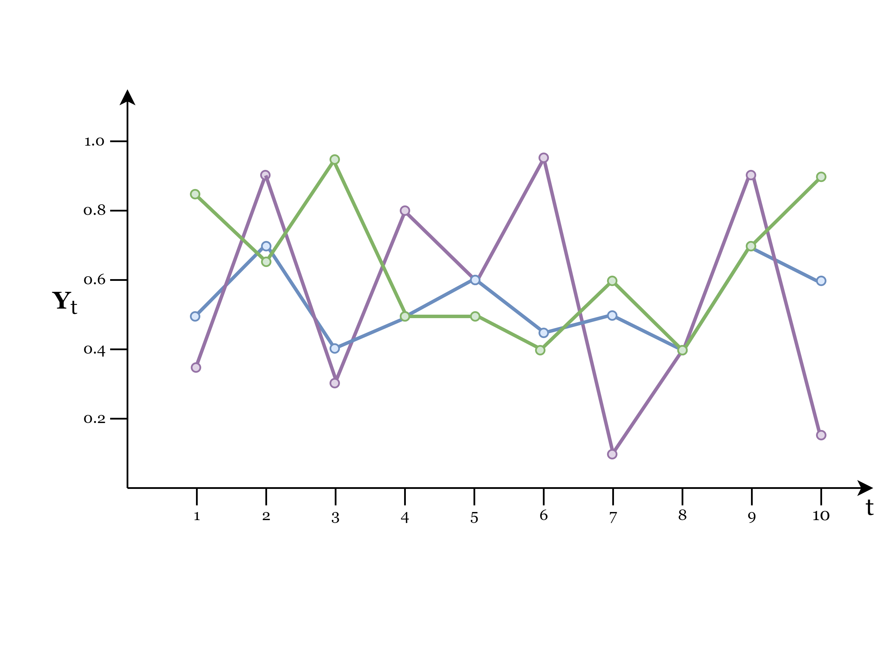
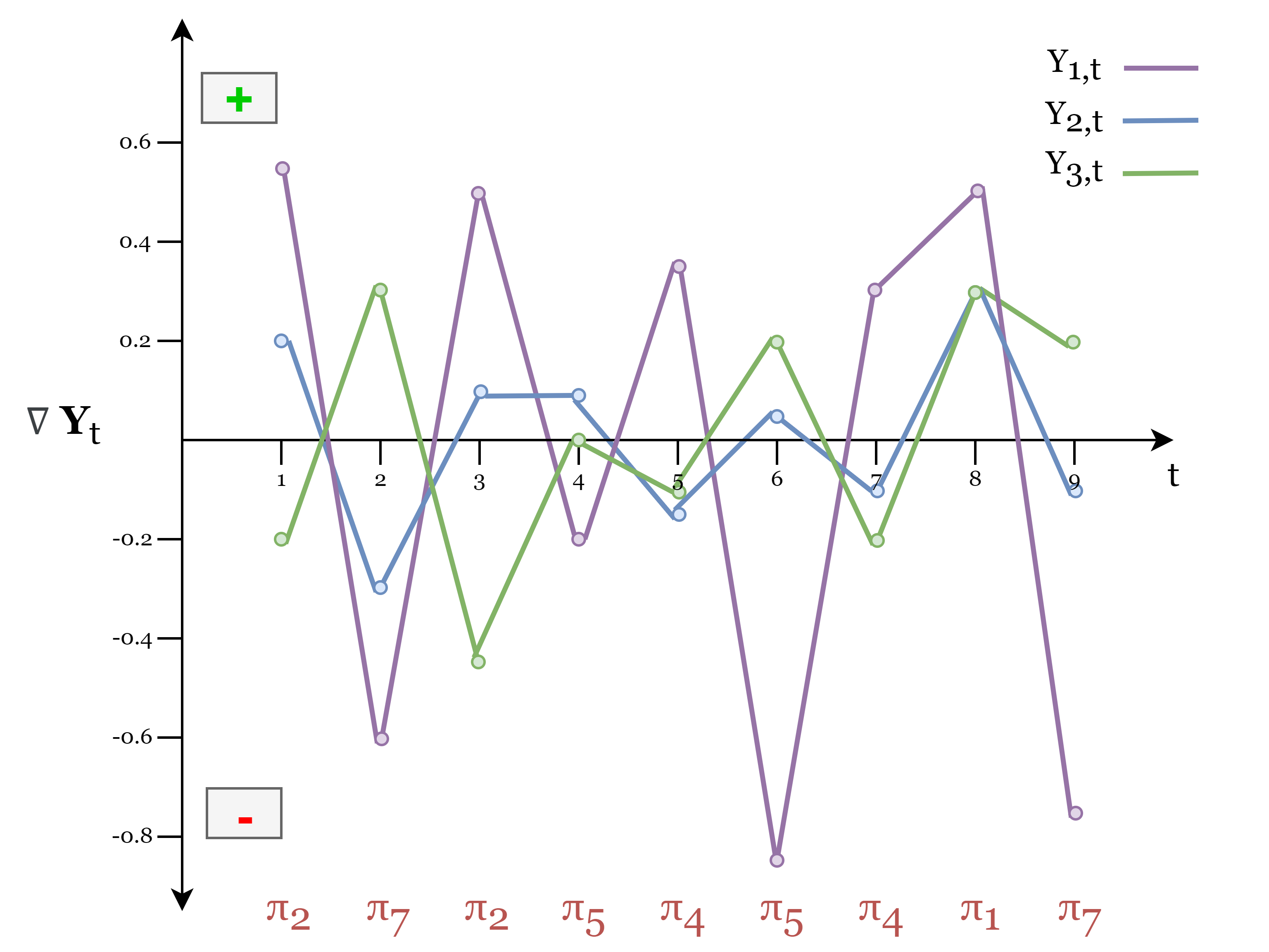
Finally, the ordinal partition transition network is the network with $2^{m}$ nodes representing the patterns $\pi_{j}$ and with directed weighted edges $(v_{i},v_{j},w_{i,j})$ established based on frequency of the transitions from pattern $\pi_{i}$ to pattern $\pi_{j}.$ In Zhang et al., 2017a , the authors also propose a measure of entropy to characterize ordinal partition transition dynamics, useful for capturing local geometric changes of trajectories. Those authors have shown that for periodic multivariate time series, with different combinations of periods, the resulting network presents clear evidence of possible forbidden patterns and so the network has several disconnected nodes. This shows determinism of the time series, while random uniform noise multivariate time series are mapped into a complete connected graph.

Guo and co-authors (Guo et al.,, 2018) propose the cross ordinal pattern transition network and the joint ordinal pattern transition networks in order to compare the relative rate of change between the two processes by the signs of $(\nabla Y_{i_{1},t}-\nabla Y_{i_{2},t})$ or $(\nabla Y_{i_{1},t}\cdot\nabla Y_{i_{2},t})$, respectively. Note that the last sign is related to the signs of changes in the component series while the former is related to amplitude of the changes.

Recently, Ruan and co-authors (Ruan et al.,, 2019) proposed a method of ordinal partition transition networks to analyze bivariate time series, $\{Y_{i,t}\}_{i=1}^{2},$ based on the initial method proposed for the analysis of univariate series (see Subsection 3.2.2). The method consists in generating the ordinal partition transition network (following the algorithm presented in Subsection 3.2.2) for each time series $Y_{1,t}$ and $Y_{2,t}$ and extracting the successive sequence of ordinal patterns of each series, removing self-transitions (self-loops in the network). Having the two sequences of ordinal patterns $\pi_{i}^{Y_{1,t}}$ and $\pi_{j}^{Y_{2,t}},$ as shown in Figure 12a, the next step is to calculate at each time $t$ the frequencies of co-occurrence of the ordinal patterns of $Y_{1,t}$ with the ordinal patterns of $Y_{2,t+h}$ i.e., $p(\pi_{j}^{Y_{2,t+h}}|\pi_{i}^{Y_{1,t}})$. In particular, when $h=0$ we analyze the simultaneous co-occurrence of ordinal patterns and when $h\neq 0$ we analyze the possible indications of causal relationships between the two systems. The resulting network have two different types of nodes corresponding to the ordinal patterns $\pi_{i}^{Y_{1,t}}$ of $Y_{1,t}$ and $\pi_{j}^{Y_{2,t}}$ of $Y_{2,t},$ respectively, and have directed and weighted edges $(\pi_{i}^{Y_{1,t}},\pi_{j}^{Y_{2,t}},w_{i,j})$ with $w_{i,j}=p(\pi_{j}^{Y_{2,t+h}}|\pi_{i}^{Y_{1,t}}).$ This results in a bipartite  OPTN (Figure 12b).

(a) Toy bivariate time series and sequence of ordinal patterns

(b) Bipartite OPTN

Figure 12: (a) Illustrative example of a toy bivariate time series ($Y_{1,t},Y_{2,t}$) and its ordinal pattern definitions and evolution. We show an embedding in a 3-dimensional space using a time delay $\tau=2$ and the schematic illustration of the OPTN analysis of the two series of ordinal patterns with a unidirectional coupling $Y_{1,t}\to Y_{2,t}$ with a coupling delay of $h=1$. The time-lagged conditional co-occurrences of the patterns $\pi_{i}^{Y_{1,t}}$ and $\pi_{j}^{Y_{2,t+h}}$ are indicated by dashed arrows. (b) The network generated by the ordinal partition transition algorithm proposed in Ruan et al., (2019).

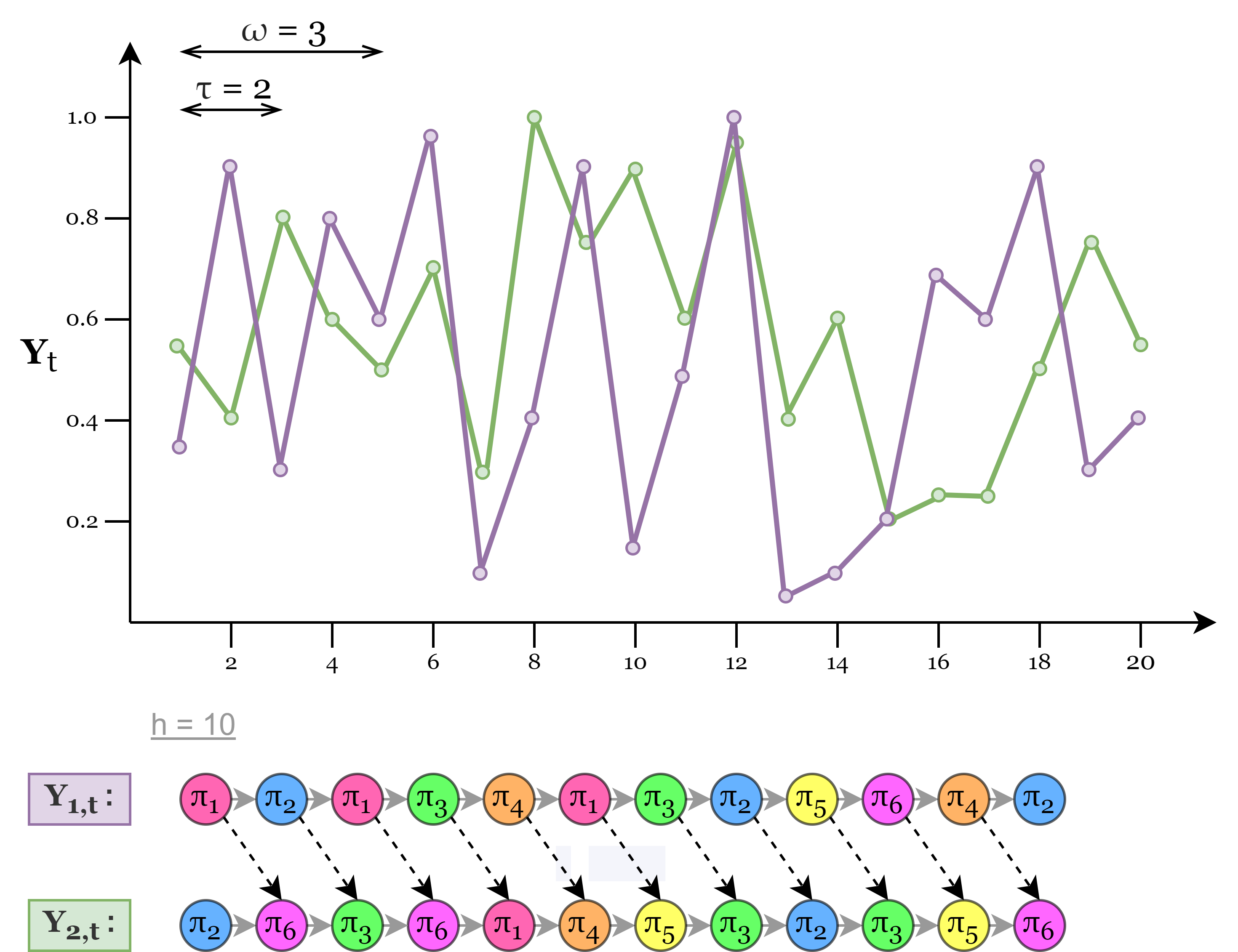
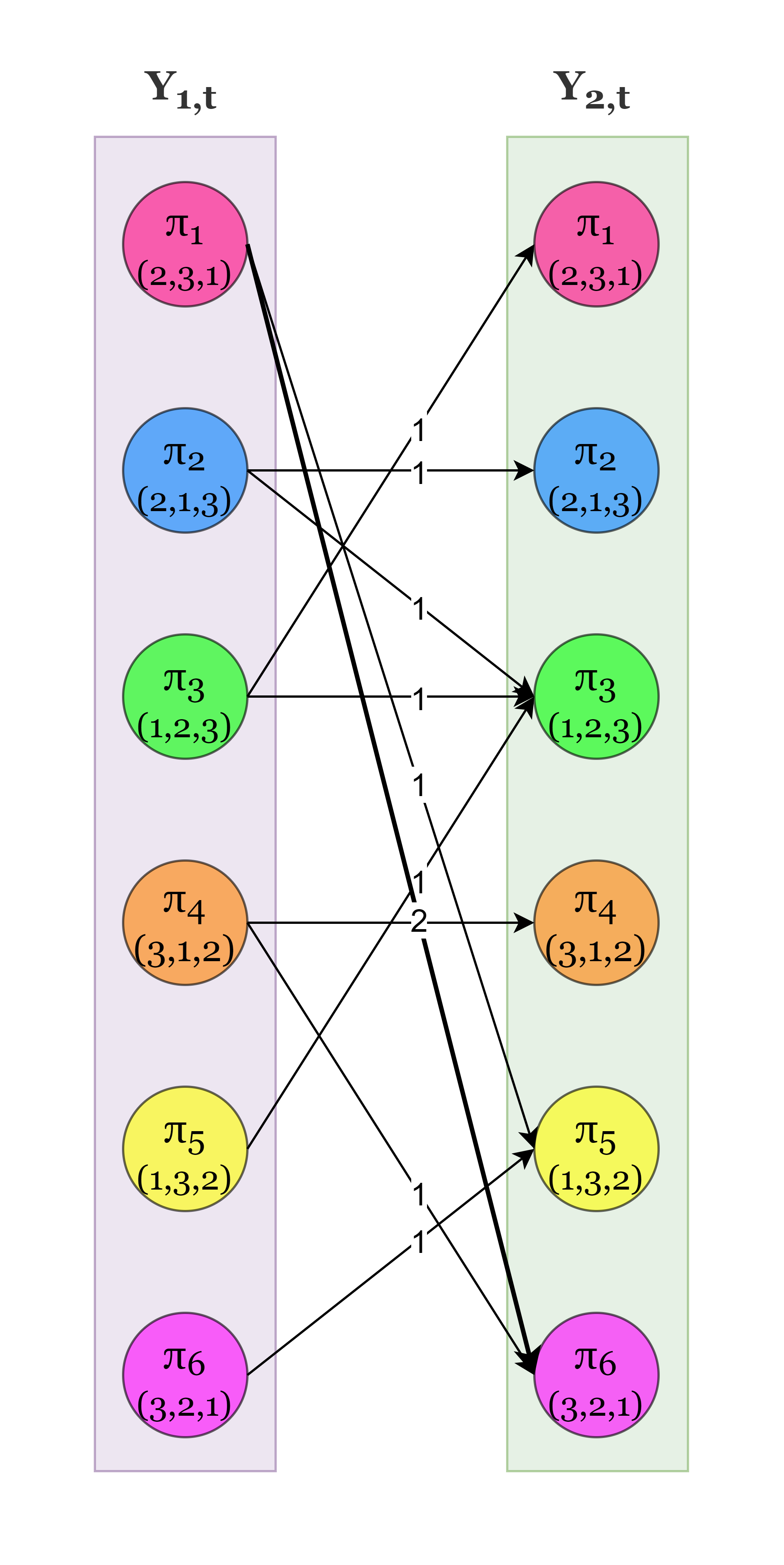
Compared to the univariate case, the bipartite OPTN measures co-occurrence probabilities between symbols in two series rather than succession probabilities of symbols in a single time series. Ruan and co-authors (Ruan et al.,, 2019) have also introduced a set of OPTN based complexity measures to infer the coupling direction and infer causality between two systems. Those authors used these measures in several coupled stochastic processes and in climate time series.

4.5 Pattern Interdependent Networks

Based on the visibility graphlets networks (Subsection 3.2.4) recently, Ren et al., (2020) proposed the pattern interdependent networks to represent the cross-correlation patterns in a stationary bivariate time series, $\{Y_{i,t}\}_{i=1}^{2}$. The method consists in generating the state chain network (following the algorithm presented in 3.2.4) for each time series component, resulting in a bi-graphlet series:

$$\left(\begin{smallmatrix}G_{1}^{[1]}\to G_{2}^{[1]}\to\ldots\to G_{T-w+1}^{[1]}\\ G_{1}^{[2]}\to G_{2}^{[2]}\to\ldots\to G_{T-w+1}^{[2]}\end{smallmatrix}\right).$$

Similar to visibility graphlets networks, all unique graphlets $G_{i}$ are identified. From all the co-occurrent pairs $G_{k}^{[1]}$ and $G_{k}^{[2]},$ with $k=1,2,\ldots,T-w+1,$ the graphlet co-occurrent frequency matrix, $\boldsymbol{A},$ is generated by calculating the co-occurrent frequencies of all the possible pairs of the unique graphlets, where the element $A_{i,j}$ represents the occurring frequency of $\left(\begin{smallmatrix}G_{i}\\ G_{j}\end{smallmatrix}\right)$ in $\left(\begin{smallmatrix}G_{k}^{[1]}\\ G_{k}^{[2]}\end{smallmatrix}\right).$ $\boldsymbol{A}$ represents a bipartite network where the rows correspond to the total of unique graphlets (nodes) across the time series $Y_{1,t}$ and the columns to the unique graphlets (nodes) across the $Y_{2,t},$ and the edges are only established between different node types (similar to the bipartite OPTN illustrated in Figure 12b). Since the sets of nodes, unique graphlets $G_{i}$ of each time series, are identical, they are merged and the bipartite network is converted into a directed and weighted network that represents the co-occurrent relationships between the unique visibility graphlets.

Ren and co-authors (Ren et al.,, 2020) applied this method to synthetic bivariate time series and showed that a set of unique graphlets and the topological structure of the resulting networks is determined and dependent on the cross-correlation, and that the differences in features, such as Hurst exponent, of the time series components determine the symmetry of the edges of the network.

4.6 Inter-System Recurrence Networks

Two extensions of recurrence networks (Subsection 3.3.3) have been proposed in the literature, one directed to bivariate time series and the other to multivariate time series (Feldhoff et al.,, 2012, 2013). As in recurrence-based methods for univariate time series, we embed each time series $Y_{\alpha,t}$ with $\alpha=1,\ldots,m$ in a $w$-dimensional, defining a set of vectors $\vec{z}_{i}^{[\alpha]}$ ($i=1,\ldots,N_{\alpha}$).

Cross-recurrence networks are based on cross-recurrence plots that aim to compare the dynamics of two time series $Y_{\alpha,t}$ and $Y_{\beta,t}$ in the same phase space (Zbilut et al.,, 1998; Marwan and Kurths,, 2002). So, both time series are simultaneously embedded in the same phase space and the cross-recurrence plot is defined by the matrix $\boldsymbol{CR}^{[\alpha\beta]}$ with elements (Marwan and Kurths,, 2002):

$$CR^{[\alpha\beta]}=\left\{\begin{array}[]{l}1\quad\textrm{if }\|\vec{z}_{i}^{[\alpha]}-\vec{z}_{j}^{[\beta]}\|\leq\varepsilon\\ 0\quad\textrm{otherwise}\\ \end{array}\right.,$$ (27)

where $i=1,\ldots,N_{\alpha},$ $j=1,\ldots,N_{\beta},$ and $\varepsilon$ is a distance threshold in the joint phase space of both processes. $\boldsymbol{CR}^{[\alpha\beta]}$ is asymmetric, since $\|\vec{z}_{i}^{[\alpha]}-\vec{z}_{j}^{[\beta]}\|=\|\vec{z}_{i}^{[\beta]}-\vec{z}_{j}^{[\alpha]}\|$ does not hold for all $i,j,\alpha,\beta,$ and it can be non-square if we consider time series of different lengths, $N_{\alpha}\neq N_{\beta}.$ This matrix can represent the adjacency matrix of a bipartite graph, corresponding to the cross-recurrence network, where the nodes belong to two distinct groups, namely, the state vectors $\{\vec{z}_{i}^{[\alpha]}\}$ and $\{\vec{z}_{j}^{[\beta]}\}$ and the edges are established only between nodes of different groups.

Inter-system recurrence networks $\boldsymbol{IR}$ arise from the combination of the recurrence matrices $\boldsymbol{R}^{[\alpha]}$ (for univariate time series $Y_{\alpha,t}$), with the cross-recurrence matrix $\boldsymbol{CR}^{[\alpha\beta]}$ (Feldhoff et al.,, 2012):

$$\boldsymbol{IR}=\left(\begin{array}[]{cccc}\boldsymbol{R}^{[1]}&\boldsymbol{CR}^{[12]}&\ldots&\boldsymbol{CR}^{[1m]}\\ \boldsymbol{CR}^{[21]}&\boldsymbol{R}^{[2]}&\ldots&\boldsymbol{CR}^{[2m]}\\ \vdots&\vdots&\ddots&\vdots\\ \boldsymbol{CR}^{[m1]}&\boldsymbol{CR}^{[m2]}&\ldots&\boldsymbol{R}^{[m]}\end{array}\right).$$ (28)

The adjacency matrix of an inter-system recurrence network is defined as

$$\boldsymbol{A}=\boldsymbol{IR}-\boldsymbol{I}_{N},$$ (29)

where $\boldsymbol{I}$ is an identity matrix of size $N=\sum_{\alpha=1}^{m}N_{\alpha}$. This results in undirected and unweighted simple graph, where the nodes and edges obey a natural partition: subgraphs $G_{\alpha}$ correspond to $\boldsymbol{R}^{[\alpha]}$ (intra-system connectivity) and subgraphs $G_{\alpha\beta}$ to $\boldsymbol{CR}^{[\alpha\beta]}$ that includes only edges between nodes from different systems (inter-system connectivity). Note that the definition of closeness can vary between different pairs of systems (Zou et al.,, 2019) if we consider different thresholds $\varepsilon_{\alpha\beta}$ for all $\alpha,\beta=1,\ldots,m.$

Inter-system recurrence networks can be analyzed as a network of networks where the nodes represent subgraphs $G_{\alpha}.$ As such and in line with previous work for the univariate case, Donges and co-authors (Donges et al., 2011b, ) used specific graph measures as discrete approximations of more general geometric properties to study the interconnections between systems. These measures proved to be useful to coupling detection from two paleoclimate records (Feldhoff et al.,, 2012), distinguish between the dynamics of focal and non-focal EEG signals (Subramaniyam and Hyttinen,, 2015) and characterize different oil–water flow patterns from multi-channel measurements (Gao et al.,, 2013; Gao et al., 2016b, ).

4.7 Joint Recurrence Networks

Joint recurrence network is another extension of the recurrence networks. The difference for the networks introduced in the previous subsection is that joint recurrence networks study the recurrence of different time series in their individual phase spaces, contrary the same phase space. The joint recurrence matrix $\boldsymbol{JR}$ is defined as follows (Romano et al.,, 2004):

$$JR=\left\{\begin{array}[]{l}1\quad\textrm{if }\|\vec{z}_{i}^{[\alpha]}-\vec{z}_{j}^{[\alpha]}\|\leq\varepsilon_{\alpha},\ \alpha=1,\ldots,m\\ 0\quad\textrm{otherwise}\\ \end{array}\right.,$$ (30)

where $\varepsilon_{\alpha}$ is the selected distance threshold for the individual time series $Y_{\alpha,t}.$ This matrix can be seen as the adjacency matrix $\boldsymbol{A}$ of a joint recurrence network:

$$\boldsymbol{A}=\boldsymbol{JR}-\boldsymbol{I}_{N},$$ (31)

where $\boldsymbol{I}$ is an identity matrix of size $N=\sum_{\alpha=1}^{m}N_{\alpha}.$ $\boldsymbol{A}$ represents the joint probability of $m$ simultaneous recurrences ($\|\vec{z}_{i}^{[\alpha]}-\vec{z}_{j}^{[\alpha]}\|,$ $\alpha=1,\ldots,m$) in the phase spaces (Marwan et al.,, 2007). Joint recurrence networks are undirected and unweighted simple graphs. They can be constructed for time series with different phase spaces and require simultaneous observations, i.e., time series of the same length. So, unlike the recurrence networks and inter-system recurrence networks, the time information is taken into account. This type of network can be analyzed from the same point of view of the recurrence networks for univariate time series, however, need to be reinterpreted in terms of the underlying joint recurrence structure (Feldhoff et al.,, 2013). Note that joint recurrence networks are similar in construction to multiplex recurrence networks, as we will see in Subsection 4.9, except that the former do not establish inter-layer edges (Zou et al.,, 2019).

This method has been successfully used to detect generalized synchronization in time series (Feldhoff et al.,, 2013). It is expected that joint recurrence will be increasingly unlikely with an increase in the number $m$ of processes. Therefore, Donner and co-authors (Donner et al.,, 2015) proposed a version called $f$-joint recurrence networks that reduces the requirement of occurrence of simultaneous recurrences in all subsystems.

4.8 Multiplex Visibility Networks

Based on the visibility methods of Section 3.1 and the definition of multilayer networks, Lacasa and co-authors (Lacasa et al.,, 2015) proposed an extension of the visibility mapping method for multivariate series analysis. The networks resulting from this approach have been called multiplex visibility graphs. A multiplex visibility graph $M$ of $m$ layers is constructed so that each layer $\alpha$ corresponds to the NVG (Section 3.1) associated with the series $Y_{\alpha,t},$ as illustrated in Figure 13.

Figure 13: Illustration of multiplex natural visibility graph algorithm for a toy multivariate time series.

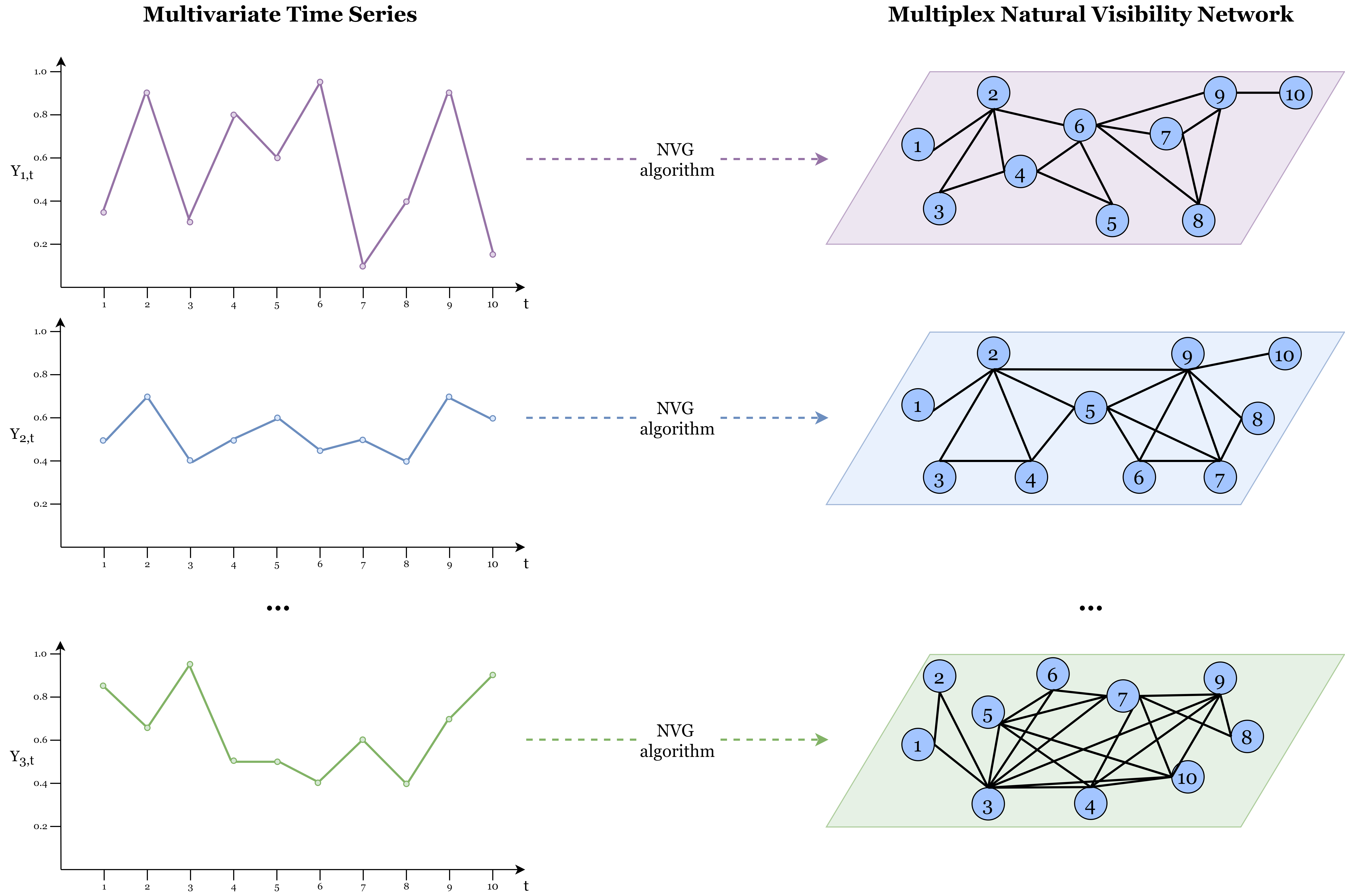
The resulting graph $M$ is now represented by the adjacency matrix vector, $\mathcal{A},$ whose elements are the adjacency matrices of the layers, $\mathcal{A}=\{\boldsymbol{A}^{[1]},\boldsymbol{A}^{[2]},\ldots,\boldsymbol{A}^{[m]}\}$ with $A^{[\alpha]}_{i,j}=1$ if and only if the node $v_{i}$ and node $v_{j}$ are connected by an edge in layer $\alpha.$

A graph of layers (or network of networks) can be built by projecting the original multiplex visibility network into a (single layer) weighted graph of $m$ nodes, where each node represents one layer. The edge weights denote a relation measure between layers, e.g., the magnitude of mutual information (Lacasa et al.,, 2015) calculated by interlayer mutual information . We should note that the construction of multiplex visibility networks can be based on any of the visibility algorithms for univarite time series mentioned in Section 3.1.

The multiplex structure was used for the study of cellular networks of diffusively coupled maps lattices (CML) (Lacasa et al.,, 2015), to model spatio-temporal complex dynamics. They show that multiplex visibility graphs allow to quantify the amount of information flow between different series through the interlayer mutual information metric, and also to distinguish between different signal behaviors, between chaotic, periodic and multiband patterns. The analysis of this metric allowed locating data points of change between different patterns of behavior of a system.

Bianchi and co-authors (Bianchi et al.,, 2017) used multiplex visibility networks method based on the weighted HVG algorithm (Subsection 3.1.5) where the edge weights are given by: $w_{i,j}=1/\sqrt{(j-i)^{2}+(Y_{i}-Y_{j})^{2}}$, incorporating temporal and amplitude information of the data. They studied topological measures of the networks to characterize neuron activations. For example, in certain types of neuronal activities the local clustering coefficient of the corresponding nodes at the moment of the activity have high values which are replicated by the same nodes in the remaining layers. This type of metrics allows to identify neuronal activities and the propagation of this activity by different neurons. Another set of real data studied using these networks were the fMRI series (Sannino et al.,, 2017) that are of extreme importance for the diagnosis of mental and neurological diseases. The results show differences in brain activities connected to psychiatric disorders.

In Gao et al., 2019a the authors studied multiplex limited penetrable horizontal visibility graphs to try to explain the difference in the accuracy of the results obtained in the task of classifying time series from individuals in normal and fatigue states. They found that some network metrics decrease in states of fatigue and that, consequently, there is less efficiency in the global information transfer. They concluded, therefore, that this transfer loss leads to a reduction in the accuracy of the classification between individuals in normal state and in fatigue.

4.9 Multiplex Recurrence Networks

Recently, Eroglu and co-authors (Eroglu et al.,, 2018), motivated by the idea that recurrences are a fingerprint of the characteristic properties of dynamic systems, the results from recurrence networks, the current and ever greater need for analysis and exploration of large amounts of data, and the previous method, multiplex visibility networks, proposed by Lacasa and co-authors (Lacasa et al.,, 2015), proposed recurrence networks for the domain of multivariate time series, the so-called multiplex recurrence networks. The algorithm follows exactly the same process as the multiplex visibility graphs presented in Section 4.8, but using recurrence networks presented in  3.3.3 instead of the visibility graphs. Remembering, the quantities of interlayer mutual information allows us to deduce a weighted single layer network from the multiplex recurrence network.

Eroglu and co-authors (Eroglu et al.,, 2018), used metrics as the interlayer mutual information and the average edge overlap  in the multiplex network and also weighted network metrics, clustering coefficient and average path length, in the weighted single layer network, in order to detect the transitions between different dynamical regimes in coupled map lattices and real world paleoclimate time series. They show that all the metrics capture similarities in the topological structures of the $m$ recurrence networks. In particular, high values of the first three metrics have been obtained for periodic behaviors, while lower values have been obtained to the chaotic behaviors. Additionally, average path length showed the opposite behavior.

In Gao et al., 2019b , the authors propose to combine the multiplex recurrence networks and deep learning techniques to detect driver fatigue in the EEG signals of subjects under alert and fatigue states. They construct a multiplex recurrence network from the EEG signal, used convolutional neural networks to extract and learn the features of the multiplex networks, and they perform a classification task. Those authors showed that this combination can achieve a high accuracy, and better results than traditional methods.

5 Conclusions

In this review we present several algorithms proposed in the literature to map univariate and multivariate time series into the complex network domain with the aim of producing new insights and overcome open issues in time series analysis, such as high-dimensionality, finding periodicities, classifying different dynamic processes, among others. For univariate time series there is a large body of literature and the mappings may be classified according to three main underlying concepts: visibility, transition and proximity.

Visibility concepts map times series into graphs with nodes representing time stamps and edges defined by a geometric relationship between data values. The graph reflects both local and global properties of the time series, especially via local maxima. Visibility-based mapping methods do not require preprocessing of the time series data. They are also completely parameter-free, except for the limited and parametric versions. These networks have become very popular in the literature due to the fact that the geometric criteria associated to visibility mappings are intuitive and easy to understand.

Intuitively, transition networks represent the transition pattern of a time series based on different types of symbolic encoding of the data. With exception to time series with clear trending behavior, these networks are not explicit about the underlying time order since time series with sharp trend behavior are mapped into quantile graphs that are chain graphs allowing us to perceive the time order of the data. The construction of these networks involves the definition of symbols representing quantiles, order patterns or different dynamic states, requiring the choice of parameters that must balance the loss of information induced by the partitioning.

The proximity networks represent the similarity of sliding windows of data over time, thus, reflecting how local properties of the time series evolve over time. The construction of proximity networks involves the definition of states of the time series as vectors, such as cycles or vectors in a phase space, requiring the selection of parameters. The resulting networks have nodes that represent these states of the time series and edges that are established using measures of similarity or distance between the states, with or without thresholding. The construction of transition and of proximity networks thus requires choosing several parameters that may influence the resulting graph and consequently the analysis of the time series. These networks are quite popular in the study of dynamical systems.

Several approaches to map multivariate time series into complex networks have been developed. Most focus on the idea of constructing a single layer network from multivariate time series, capable of capturing dependencies between the component processes, both contemporary and lagged, as well as the serial dependencies. However, with technological advances and the growing need to analyze complex and high-dimensional data, new techniques have emerged, namely, methods that give rise to high-level structures: multiple layers networks. Although preliminary, this type of multivariate time series mapping has an important characteristic: all the methods developed for the univariate context can be extended to the context of multilayer networks, allowing the reuse of knowledge already acquired in the univariate case.

A network science approach to time series analysis has been used in different application domains and allowed to characterize system dynamics, to distinguish different dynamics, to identify regime shifts and dynamical transitions, to test for reversibility and to forecast. This survey hints at the conclusion that this approach provides complementary information to traditional time series analysis. This approach can be leveraged to address existing fundamental open issues. Among them we highlight the following: missing values, unequally spaced data, visualization of high-dimensional data, time series classification and clustering. Data recorded using electronic devices such as sensors are prone to missing values and conventional imputation methods may cause bias in the data. The work of Donner and Donges, (2012) addresses this problem of missing values via a network perspective and, although the results are preliminary, they highlight a path to the solution of this issue. Unequally spaced data collected over time occurs frequently for several reasons, hindering the application of time series analysis methodology. The most common approach to this issue is data aggregation which leads to the loss of information. As far as we know, this problem has not yet been addressed from the point of view of networks. Visualization of high dimensional temporal data is a practical issue to whose solution may contribute strategies to reduce the dimensionality of the data by using suitable mapping methods (e.g. quantile graphs). Mining time large collections of time series data is increasingly accomplished via time series features, e.g. trend, length of time series, strength of trend, autocorrelations (Kang et al.,, 2017). The features extracted from the time series networks may be added to the classical set of time series features to enhance the data characterization. In particular, Silva, (2018) has shown that network metrics can be used to accurately cluster time series from different models, a relevant important contribution to time series mining.

There is still much potential to be explored and this survey aims precisely to equip the reader with the knowledge capable of unveiling this potential.

References

- Ahmadlou et al., (2010) Ahmadlou, M., Adeli, H., and Adeli, A. (2010). New diagnostic EEG markers of the alzheimer’s disease using visibility graph. Journal of Neural Transmission, 117(9):1099–1109.
- Albert and Barabási, (2002) Albert, R. and Barabási, A.-L. (2002). Statistical mechanics of complex networks. Reviews of Modern Physics, 74(1):47.
- Amigó et al., (2007) Amigó, J. M., Zambrano, S., and Sanjuán, M. A. (2007). True and false forbidden patterns in deterministic and random dynamics. EPL (Europhysics Letters), 79(5):50001.
- An et al., (2019) An, P., Si, W., Ding, S., Xue, G., and Yuan, Z. (2019). A novel EEG sleep staging method for wearable devices based on amplitude-time mapping. In 2019 IEEE 4th International Conference on Advanced Robotics and Mechatronics (ICARM), pages 124–129. IEEE.
- Baggio and Sainaghi, (2016) Baggio, R. and Sainaghi, R. (2016). Mapping time series into networks as a tool to assess the complex dynamics of tourism systems. Tourism Management, 54:23–33.
- Barabási and Albert, (1999) Barabási, A.-L. and Albert, R. (1999). Emergence of scaling in random networks. Science, 286(5439):509–512.
- Barabási, (2016) Barabási, A.-L. (2016). Network Science. Cambridge University Press.
- Barigozzi and Brownlees, (2019) Barigozzi, M. and Brownlees, C. (2019). Nets: Network estimation for time series. Journal of Applied Econometrics, 34(3):347–364.
- Barigozzi and Hallin, (2016) Barigozzi, M. and Hallin, M. (2016). Generalized dynamic factor models and volatilities: recovering the market volatility shocks.
- Barigozzi and Hallin, (2017) Barigozzi, M. and Hallin, M. (2017). A network analysis of the volatility of high dimensional financial series. Journal of the Royal Statistical Society: Series C (Applied Statistics), 66(3):581–605.
- Bezsudnov and Snarskii, (2014) Bezsudnov, I. and Snarskii, A. (2014). From the time series to the complex networks: The parametric natural visibility graph. Physica A: Statistical Mechanics and its Applications, 414:53–60.
- Bianchi et al., (2017) Bianchi, F. M., Livi, L., Alippi, C., and Jenssen, R. (2017). Multiplex visibility graphs to investigate recurrent neural network dynamics. Scientific Reports, 7:44037.
- Boccaletti et al., (2014) Boccaletti, S., Bianconi, G., Criado, R., Del Genio, C. I., Gómez-Gardenes, J., Romance, M., Sendina-Nadal, I., Wang, Z., and Zanin, M. (2014). The structure and dynamics of multilayer networks. Physics Reports, 544(1):1–122.
- Bonanno et al., (2004) Bonanno, G., Caldarelli, G., Lillo, F., Micciche, S., Vandewalle, N., and Mantegna, R. N. (2004). Networks of equities in financial markets. The European Physical Journal B, 38(2):363–371.
- Box et al., (2015) Box, G. E., Jenkins, G. M., Reinsel, G. C., and Ljung, G. M. (2015). Time Series Analysis: Forecasting and Control. John Wiley & Sons.
- Bradley and Kantz, (2015) Bradley, E. and Kantz, H. (2015). Nonlinear time-series analysis revisited. Chaos: An Interdisciplinary Journal of Nonlinear Science, 25(9):097610.
- Bullmore and Sporns, (2009) Bullmore, E. and Sporns, O. (2009). Complex brain networks: graph theoretical analysis of structural and functional systems. Nature Reviews Neuroscience, 10(3):186.
- Cai et al., (2010) Cai, S.-M., Zhou, Y.-B., Zhou, T., and Zhou, P.-L. (2010). Hierarchical organization and disassortative mixing of correlation-based weighted financial networks. International Journal of Modern Physics C, 21(03):433–441.
- Campanharo et al., (2018) Campanharo, A. S., Doescher, E., and Ramos, F. M. (2018). Application of quantile graphs to the automated analysis of EEG signals. Neural Processing Letters, 52:5–20.
- Campanharo and Ramos, (2016) Campanharo, A. S. and Ramos, F. M. (2016). Hurst exponent estimation of self-affine time series using quantile graphs. Physica A: Statistical Mechanics and its Applications, 444:43–48.
- Campanharo et al., (2011) Campanharo, A. S., Sirer, M. I., Malmgren, R. D., Ramos, F. M., and Amaral, L. A. N. (2011). Duality between time series and networks. PLOS ONE, 6(8):e23378.
- Campanharo, (2016) Campanharo, Andriana SLO, F. M. (2016). Quantile graphs for the characterization of chaotic dynamics in time series. In WCCS 2015 – IEEE Third World Conference on Complex Systems. IEEE.
- Cao et al., (2004) Cao, Y., Tung, W.-w., Gao, J., Protopopescu, V. A., and Hively, L. M. (2004). Detecting dynamical changes in time series using the permutation entropy. Physical Review E, 70(4):046217.
- Charakopoulos et al., (2014) Charakopoulos, A., Karakasidis, T., Papanicolaou, P., and Liakopoulos, A. (2014). The application of complex network time series analysis in turbulent heated jets. Chaos: An Interdisciplinary Journal of Nonlinear Science, 24(2):024408.
- Costa et al., (2011) Costa, L. d. F., Oliveira Jr, O. N., Travieso, G., Rodrigues, F. A., Villas Boas, P. R., Antiqueira, L., Viana, M. P., and Correa Rocha, L. E. (2011). Analyzing and modeling real-world phenomena with complex networks: A survey of applications. Advances in Physics, 60(3):329–412.
- Costa et al., (2007) Costa, L. d. F., Rodrigues, F. A., Travieso, G., and Villas Boas, P. R. (2007). Characterization of complex networks: A survey of measurements. Advances in Physics, 56(1):167–242.
- Diebold and Yılmaz, (2014) Diebold, F. X. and Yılmaz, K. (2014). On the network topology of variance decompositions: Measuring the connectedness of financial firms. Journal of Econometrics, 182(1):119–134.
- Dijkstra et al., (2019) Dijkstra, H. A., Hernández-García, E., Masoller, C., and Barreiro, M. (2019). Networks in Climate. Cambridge University Press.
- Donges et al., (2013) Donges, J. F., Donner, R. V., and Kurths, J. (2013). Testing time series irreversibility using complex network methods. EPL (Europhysics Letters), 102(1):10004.
- (30) Donges, J. F., Donner, R. V., Rehfeld, K., Marwan, N., Trauth, M. H., and Kurths, J. (2011a). Identification of dynamical transitions in marine palaeoclimate records by recurrence network analysis. Nonlinear Processes in Geophysics, 18(5):545–562.
- Donges et al., (2012) Donges, J. F., Heitzig, J., Donner, R. V., and Kurths, J. (2012). Analytical framework for recurrence network analysis of time series. Physical Review E, 85(4):046105.
- (32) Donges, J. F., Schultz, H. C., Marwan, N., Zou, Y., and Kurths, J. (2011b). Investigating the topology of interacting networks. The European Physical Journal B, 84(4):635–651.
- Donner and Donges, (2012) Donner, R. V. and Donges, J. F. (2012). Visibility graph analysis of geophysical time series: Potentials and possible pitfalls. Acta Geophysica, 60(3):589–623.
- Donner et al., (2015) Donner, R. V., Donges, J. F., Zou, Y., and Feldhoff, J. H. (2015). Complex network analysis of recurrences. In Recurrence Quantification Analysis, pages 101–163. Springer.
- (35) Donner, R. V., Heitzig, J., Donges, J. F., Zou, Y., Marwan, N., and Kurths, J. (2011a). The geometry of chaotic dynamics—a complex network perspective. The European Physical Journal B, 84(4):653–672.
- (36) Donner, R. V., Small, M., Donges, J. F., Marwan, N., Zou, Y., Xiang, R., and Kurths, J. (2011b). Recurrence-based time series analysis by means of complex network methods. International Journal of Bifurcation and Chaos, 21(04):1019–1046.
- Donner et al., (2010) Donner, R. V., Zou, Y., Donges, J. F., Marwan, N., and Kurths, J. (2010). Recurrence networks — a novel paradigm for nonlinear time series analysis. New Journal of Physics, 12(3):033025.
- Douc et al., (2014) Douc, R., Moulines, E., and Stoffer, D. (2014). Nonlinear Time Series: Theory, Methods and Applications with R Examples. Chapman and Hall/CRC, 1 edition.
- Eckmann et al., (1987) Eckmann, J., Kamphorst, S. O., and Ruelle, D. (1987). Recurrence plots of dynamical systems. Europhysics Letters (EPL), 4(9):973––977.
- Eguiluz et al., (2005) Eguiluz, V. M., Chialvo, D. R., Cecchi, G. A., Baliki, M., and Apkarian, A. V. (2005). Scale-free brain functional networks. Physical Review Letters, 94(1):018102.
- Elsner et al., (2009) Elsner, J., Jagger, T., and Fogarty, E. (2009). Visibility network of united states hurricanes. Geophysical Research Letters, 36(16):L16702.
- Epskamp and Fried, (2018) Epskamp, S. and Fried, E. I. (2018). A tutorial on regularized partial correlation networks. Psychological Methods, 23(4):617.
- Erdős and Rényi, (1960) Erdős, P. and Rényi, A. (1960). On the evolution of random graphs. Publ. Math. Inst. Hung. Acad. Sci, 5(1):17–60.
- Eroglu et al., (2018) Eroglu, D., Marwan, N., Stebich, M., and Kurths, J. (2018). Multiplex recurrence networks. Physical Review E, 97(1):012312.
- Feldhoff et al., (2013) Feldhoff, J., Donner, R. V., Donges, J. F., Marwan, N., and Kurths, J. (2013). Geometric signature of complex synchronisation scenarios. EPL (Europhysics Letters), 102(3):30007.
- Feldhoff et al., (2012) Feldhoff, J. H., Donner, R. V., Donges, J. F., Marwan, N., and Kurths, J. (2012). Geometric detection of coupling directions by means of inter-system recurrence networks. Physics Letters A, 376(46):3504–3513.
- Feng and He, (2017) Feng, C. and He, B. (2017). Construction of complex networks from time series based on the cross correlation interval. Open Physics, 15(1):253–260.
- Flanagan et al., (2019) Flanagan, R., Lacasa, L., and Nicosia, V. (2019). On the spectral properties of Feigenbaum graphs. Journal of Physics A: Mathematical and Theoretical, 53(2):025702.
- Fukino et al., (2016) Fukino, M., Hirata, Y., and Aihara, K. (2016). Coarse-graining time series data: Recurrence plot of recurrence plots and its application for music. Chaos: An Interdisciplinary Journal of Nonlinear Science, 26(2):023116.
- Gao et al., (2015) Gao, Y.-C., Zeng, Y., and Cai, S.-M. (2015). Influence network in the chinese stock market. Journal of Statistical Mechanics: Theory and Experiment, 2015(3):P03017.
- Gao and Jin, (2009) Gao, Z. and Jin, N. (2009). Complex network from time series based on phase space reconstruction. Chaos: An Interdisciplinary Journal of Nonlinear Science, 19(3):033137.
- (52) Gao, Z.-K., Cai, Q., Yang, Y.-X., Dang, W.-D., and Zhang, S.-S. (2016a). Multiscale limited penetrable horizontal visibility graph for analyzing nonlinear time series. Scientific Reports, 6(1):35622.
- (53) Gao, Z.-K., Guo, W., Cai, Q., Ma, C., Zhang, Y.-B., and Kurths, J. (2019a). Characterization of ssmvep-based EEG signals using multiplex limited penetrable horizontal visibility graph. Chaos: An Interdisciplinary Journal of Nonlinear Science, 29(7):073119.
- (54) Gao, Z.-K., Li, Y.-L., Yang, Y.-X., and Ma, C. (2019b). A recurrence network-based convolutional neural network for fatigue driving detection from EEG. Chaos: An Interdisciplinary Journal of Nonlinear Science, 29(11):113126.
- (55) Gao, Z.-K., Yang, Y.-X., Cai, Q., Zhang, S.-S., and Jin, N.-D. (2016b). Multivariate weighted recurrence network inference for uncovering oil-water transitional flow behavior in a vertical pipe. Chaos: An Interdisciplinary Journal of Nonlinear Science, 26(6):063117.
- Gao et al., (2013) Gao, Z.-K., Zhang, X.-W., Jin, N.-D., Marwan, N., and Kurths, J. (2013). Multivariate recurrence network analysis for characterizing horizontal oil-water two-phase flow. Physical Review E, 88(3):032910.
- Ghosh, (2007) Ghosh, S. K. (2007). Visibility Algorithms in the Plane. Cambridge university press.
- Guo et al., (2018) Guo, H., Zhang, J.-Y., Zou, Y., and Guan, S.-G. (2018). Cross and joint ordinal partition transition networks for multivariate time series analysis. Frontiers of Physics, 13(5):130508.
- Gutin et al., (2011) Gutin, G., Mansour, T., and Severini, S. (2011). A characterization of horizontal visibility graphs and combinatorics on words. Physica A: Statistical Mechanics and its Applications, 390(12):2421–2428.
- Holme and Saramäki, (2012) Holme, P. and Saramäki, J. (2012). Temporal networks. Physics Reports, 519(3):97–125.
- Hou et al., (2016) Hou, F., Li, F., Wang, J., and Yan, F. (2016). Visibility graph analysis of very short-term heart rate variability during sleep. Physica A: Statistical Mechanics and its Applications, 458:140–145.
- (62) Iacovacci, J. and Lacasa, L. (2016a). Sequential motif profile of natural visibility graphs. Physical Review E, 94(5):052309.
- (63) Iacovacci, J. and Lacasa, L. (2016b). Sequential visibility-graph motifs. Physical Review E, 93(4):042309.
- Iwayama et al., (2013) Iwayama, K., Hirata, Y., Suzuki, H., and Aihara, K. (2013). Change-point detection with recurrence networks. Nonlinear Theory and Its Applications, IEICE, 4(2):160–171.
- Jacob et al., (2016) Jacob, R., Harikrishnan, K., Misra, R., and Ambika, G. (2016). Can recurrence networks show small-world property? Physics Letters A, 380(35):2718–2723.
- Jacob et al., (2019) Jacob, R., Harikrishnan, K., Misra, R., and Ambika, G. (2019). Weighted recurrence networks for the analysis of time-series data. Proceedings of the Royal Society A, 475(2221):20180256.
- Kang et al., (2017) Kang, Y., Hyndman, R. J., and Smith-Miles, K. (2017). Visualising forecasting algorithm performance using time series instance spaces. International Journal of Forecasting, 33(2):345–358.
- Kaur and Singh, (2016) Kaur, M. and Singh, S. (2016). Analyzing negative ties in social networks: A survey. Egyptian Informatics Journal, 17(1):21–43.
- Kiel and Elliott, (1996) Kiel, L. D. and Elliott, E. W. (1996). Chaos Theory in the Social Sciences: Foundations and Applications. University of Michigan Press.
- Kivelä et al., (2014) Kivelä, M., Arenas, A., Barthelemy, M., Gleeson, J. P., Moreno, Y., and Porter, M. A. (2014). Multilayer networks. Journal of Complex Networks, 2(3):203–271.
- Kretschmer et al., (2016) Kretschmer, M., Coumou, D., Donges, J. F., and Runge, J. (2016). Using causal effect networks to analyze different arctic drivers of midlatitude winter circulation. Journal of Climate, 29(11):4069–4081.
- Kulp et al., (2016) Kulp, C. W., Chobot, J. M., Freitas, H. R., and Sprechini, G. D. (2016). Using ordinal partition transition networks to analyze ECG data. Chaos: An Interdisciplinary Journal of Nonlinear Science, 26(7):073114.
- Lacasa et al., (2008) Lacasa, L., Luque, B., Ballesteros, F., Luque, J., and Nuno, J. C. (2008). From time series to complex networks: The visibility graph. Proceedings of the National Academy of Sciences, 105(13):4972–4975.
- Lacasa et al., (2009) Lacasa, L., Luque, B., Luque, J., and Nuno, J. C. (2009). The visibility graph: A new method for estimating the hurst exponent of fractional brownian motion. EPL (Europhysics Letters), 86(3):30001.
- Lacasa et al., (2015) Lacasa, L., Nicosia, V., and Latora, V. (2015). Network structure of multivariate time series. Scientific Reports, 5(1):15508.
- Lacasa et al., (2012) Lacasa, L., Nunez, A., Roldán, É., Parrondo, J. M., and Luque, B. (2012). Time series irreversibility: a visibility graph approach. The European Physical Journal B, 85(6):217.
- Lacasa and Toral, (2010) Lacasa, L. and Toral, R. (2010). Description of stochastic and chaotic series using visibility graphs. Physical Review E, 82(3):036120.
- Lan et al., (2015) Lan, X., Mo, H., Chen, S., Liu, Q., and Deng, Y. (2015). Fast transformation from time series to visibility graphs. Chaos: An Interdisciplinary Journal of Nonlinear Science, 25(8):083105.
- Lanne and Nyberg, (2016) Lanne, M. and Nyberg, H. (2016). Generalized forecast error variance decomposition for linear and nonlinear multivariate models. Oxford Bulletin of Economics and Statistics, 78(4):595–603.
- Li et al., (2018) Li, D., Lin, J., Bissyande, T. F. D. A., Klein, J., and Le Traon, Y. (2018). Extracting statistical graph features for accurate and efficient time series classification. In 21st International Conference on Extending Database Technology, pages 1–12.
- Liu and Zhou, (2010) Liu, C. and Zhou, W.-X. (2010). Superfamily classification of nonstationary time series based on dfa scaling exponents. Journal of Physics A: Mathematical and Theoretical, 43(49):495005.
- Liu et al., (2010) Liu, C., Zhou, W.-X., and Yuan, W.-K. (2010). Statistical properties of visibility graph of energy dissipation rates in three-dimensional fully developed turbulence. Physica A: Statistical Mechanics and its Applications, 389(13):2675–2681.
- Liu and Wang, (2018) Liu, L. and Wang, Z. (2018). Encoding temporal markov dynamics in graph for visualizing and mining time series. In Workshops at the Thirty-Second AAAI Conference on Artificial Intelligence.
- Long, (2013) Long, Y. (2013). Visibility graph network analysis of gold price time series. Physica A: Statistical Mechanics and its Applications, 392(16):3374–3384.
- Lorenz, (1963) Lorenz, E. N. (1963). Deterministic nonperiodic flow. Journal of the Atmospheric Sciences, 20(2):130–141.
- Luque et al., (2009) Luque, B., Lacasa, L., Ballesteros, F., and Luque, J. (2009). Horizontal visibility graphs: Exact results for random time series. Physical Review E, 80(4):046103.
- Lyapunov, (1892) Lyapunov, A. M. (1892). The general problem of motion stability. Annals of Mathematics Studies, 17.
- Marwan, (2008) Marwan, N. (2008). A historical review of recurrence plots. The European Physical Journal Special Topics, 164(1):3–12.
- Marwan et al., (2009) Marwan, N., Donges, J. F., Zou, Y., Donner, R. V., and Kurths, J. (2009). Complex network approach for recurrence analysis of time series. Physics Letters A, 373(46):4246–4254.
- Marwan and Kurths, (2002) Marwan, N. and Kurths, J. (2002). Nonlinear analysis of bivariate data with cross recurrence plots. Physics Letters A, 302(5-6):299–307.
- Marwan et al., (2007) Marwan, N., Romano, M. C., Thiel, M., and Kurths, J. (2007). Recurrence plots for the analysis of complex systems. Physics Reports, 438(5-6):237–329.
- McCullough et al., (2016) McCullough, M., Sakellariou, K., Stemler, T., and Small, M. (2016). Counting forbidden patterns in irregularly sampled time series. i. the effects of under-sampling, random depletion, and timing jitter. Chaos: An Interdisciplinary Journal of Nonlinear Science, 26(12):123103.
- McCullough et al., (2017) McCullough, M., Small, M., Iu, H. H.-C., and Stemler, T. (2017). Multiscale ordinal network analysis of human cardiac dynamics. Philosophical Transactions of the Royal Society A: Mathematical, Physical and Engineering Sciences, 375(2096):20160292.
- McCullough et al., (2015) McCullough, M., Small, M., Stemler, T., and Iu, H. H.-C. (2015). Time lagged ordinal partition networks for capturing dynamics of continuous dynamical systems. Chaos: An Interdisciplinary Journal of Nonlinear Science, 25(5):053101.
- Meinshausen et al., (2006) Meinshausen, N., Bühlmann, P., et al. (2006). High-dimensional graphs and variable selection with the lasso. The Annals of Statistics, 34(3):1436–1462.
- Milo et al., (2004) Milo, R., Itzkovitz, S., Kashtan, N., Levitt, R., Shen-Orr, S., Ayzenshtat, I., Sheffer, M., and Alon, U. (2004). Superfamilies of evolved and designed networks. Science, 303(5663):1538–1542.
- Milo et al., (2002) Milo, R., Shen-Orr, S., Itzkovitz, S., Kashtan, N., Chklovskii, D., and Alon, U. (2002). Network motifs: simple building blocks of complex networks. Science, 298(5594):824–827.
- Mori et al., (2016) Mori, U., Mendiburu, A., and Lozano, J. A. (2016). Distance measures for time series in R: The tsdist package. R J., 8(2):451.
- Mutua et al., (2015) Mutua, S., Gu, C., and Yang, H. (2015). Visibility graph based time series analysis. PloS one, 10(11):e0143015.
- Mutua et al., (2016) Mutua, S., Gu, C., and Yang, H. (2016). Visibility graphlet approach to chaotic time series. Chaos: An Interdisciplinary Journal of Nonlinear Science, 26(5):053107.
- Nakamura et al., (2016) Nakamura, T., Tanizawa, T., and Small, M. (2016). Constructing networks from a dynamical system perspective for multivariate nonlinear time series. Physical Review E, 93(3):032323.
- Newman, (2010) Newman, M. (2010). Networks: An Introduction. Oxford University Press.
- Newman, (2003) Newman, M. E. (2003). The structure and function of complex networks. SIAM Review, 45(2):167–256.
- (104) Nuñez, A., Lacasa, L., Valero, E., Gómez, J. P., and Luque, B. (2012a). Detecting series periodicity with horizontal visibility graphs. International Journal of Bifurcation and Chaos, 22(07):1250160.
- (105) Nuñez, A. M., Lacasa, L., Gomez, J. P., and Luque, B. (2012b). Visibility algorithms: A short review. New Frontiers in Graph Theory, pages 119–152 (Chapter 6).
- Pei et al., (2014) Pei, X., Wang, J., Deng, B., Wei, X., and Yu, H. (2014). WLPVG approach to the analysis of EEG-based functional brain network under manual acupuncture. Cognitive Neurodynamics, 8(5):417–428.
- Pesaran and Shin, (1998) Pesaran, H. H. and Shin, Y. (1998). Generalized impulse response analysis in linear multivariate models. Economics Letters, 58(1):17–29.
- Pessa and Ribeiro, (2019) Pessa, A. A. and Ribeiro, H. V. (2019). Characterizing stochastic time series with ordinal networks. Physical Review E, 100(4):042304.
- Pineda et al., (2020) Pineda, A. M., Ramos, F. M., Betting, L. E., and Campanharo, A. S. (2020). Quantile graphs for EEG-based diagnosis of alzheimer’s disease. Plos one, 15(6):e0231169.
- Porter, (2018) Porter, M. A. (2018). What is… a multilayer network. Notices of the AMS, 65(11).
- Qian et al., (2010) Qian, M.-C., Jiang, Z.-Q., and Zhou, W.-X. (2010). Universal and nonuniversal allometric scaling behaviors in the visibility graphs of world stock market indices. Journal of Physics A: Mathematical and Theoretical, 43(33):335002.
- Ravetti et al., (2014) Ravetti, M. G., Carpi, L. C., Gonçalves, B. A., Frery, A. C., and Rosso, O. A. (2014). Distinguishing noise from chaos: objective versus subjective criteria using horizontal visibility graph. PLOS ONE, 9(9):e108004.
- Ren et al., (2020) Ren, H., Yuan, Q., Semba, S., Weng, T., Gu, C., and Yang, H. (2020). Pattern interdependent network of cross-correlation in multivariate time series. Physics Letters A, 384(30):126781.
- Ren and Jin, (2020) Ren, W. and Jin, N. (2020). Sequential limited penetrable visibility-graph motifs. Nonlinear Dynamics, 99:2399––2408.
- Romano et al., (2004) Romano, M. C., Thiel, M., Kurths, J., and von Bloh, W. (2004). Multivariate recurrence plots. Physics Letters A, 330(3-4):214–223.
- Rössler, (1976) Rössler, O. E. (1976). An equation for continuous chaos. Physics Letters A, 57(5):397–398.
- Ruan et al., (2019) Ruan, Y., Donner, R. V., Guan, S., and Zou, Y. (2019). Ordinal partition transition network based complexity measures for inferring coupling direction and delay from time series. Chaos: An Interdisciplinary Journal of Nonlinear Science, 29(4):043111.
- (118) Runge, J., Bathiany, S., Bollt, E., Camps-Valls, G., Coumou, D., Deyle, E., Glymour, C., Kretschmer, M., Mahecha, M. D., Muñoz-Marí, J., et al. (2019a). Inferring causation from time series in earth system sciences. Nature Communications, 10(1):1–13.
- (119) Runge, J., Nowack, P., Kretschmer, M., Flaxman, S., and Sejdinovic, D. (2019b). Detecting and quantifying causal associations in large nonlinear time series datasets. Science Advances, 5(11):eaau4996.
- Runge et al., (2015) Runge, J., Petoukhov, V., Donges, J. F., Hlinka, J., Jajcay, N., Vejmelka, M., Hartman, D., Marwan, N., Paluš, M., and Kurths, J. (2015). Identifying causal gateways and mediators in complex spatio-temporal systems. Nature Communications, 6(1):1–10.
- Runge et al., (2014) Runge, J., Petoukhov, V., and Kurths, J. (2014). Quantifying the strength and delay of climatic interactions: The ambiguities of cross correlation and a novel measure based on graphical models. Journal of Climate, 27(2):720–739.
- Sakellariou et al., (2016) Sakellariou, K., McCullough, M., Stemler, T., and Small, M. (2016). Counting forbidden patterns in irregularly sampled time series. ii. reliability in the presence of highly irregular sampling. Chaos: An Interdisciplinary Journal of Nonlinear Science, 26(12):123104.
- Sannino et al., (2017) Sannino, S., Stramaglia, S., Lacasa, L., and Marinazzo, D. (2017). Visibility graphs for fMRI data: Multiplex temporal graphs and their modulations across resting-state networks. Network Neuroscience, 1(3):208–221.
- Shao et al., (2012) Shao, Y.-H., Gu, G.-F., Jiang, Z.-Q., Zhou, W.-X., and Sornette, D. (2012). Comparing the performance of fa, dfa and dma using different synthetic long-range correlated time series. Scientific Reports, 2:835.
- Shao, (2010) Shao, Z.-G. (2010). Network analysis of human heartbeat dynamics. Applied Physics Letters, 96(7):073703.
- Shirazi et al., (2009) Shirazi, A., Jafari, G. R., Davoudi, J., Peinke, J., Tabar, M. R. R., and Sahimi, M. (2009). Mapping stochastic processes onto complex networks. Journal of Statistical Mechanics: Theory and Experiment, 2009(07):1–11.
- Shumway and Stoffer, (2017) Shumway, R. H. and Stoffer, D. S. (2017). Time Series Analysis and its Applications. 1431-875X. Springer, 4 edition.
- Silva, (2018) Silva, V. F. (2018). Time series analysis based on complex networks. Msc thesis, University of Porto.
- Small, (2013) Small, M. (2013). Complex networks from time series: Capturing dynamics. In 2013 IEEE International Symposium on Circuits and Systems, pages 2509–2512. IEEE.
- Small et al., (2009) Small, M., Zhang, J., and Xu, X. (2009). Transforming time series into complex networks. In International Conference on Complex Sciences, volume 5, pages 2078–2089. Springer.
- Strozzi et al., (2011) Strozzi, F., Poljansek, K., Bono, F., Gutierrez, E., and Zaldivar, J. (2011). Recurrence networks: evolution and robustness. International Journal of Bifurcation and Chaos, 21(04):1047–1063.
- Subramaniyam and Hyttinen, (2015) Subramaniyam, N. P. and Hyttinen, J. (2015). Dynamics of intracranial electroencephalographic recordings from epilepsy patients using univariate and bivariate recurrence networks. Physical Review E, 91(2):022927.
- Supriya et al., (2016) Supriya, S., Siuly, S., Wang, H., Cao, J., and Zhang, Y. (2016). Weighted visibility graph with complex network features in the detection of epilepsy. IEEE Access, 4:6554–6566.
- Takens, (1981) Takens, F. (1981). Detecting strange attractors in turbulence. In Dynamical systems and turbulence, Warwick 1980, pages 366–381. Springer.
- Telesca and Lovallo, (2012) Telesca, L. and Lovallo, M. (2012). Analysis of seismic sequences by using the method of visibility graph. EPL (Europhysics Letters), 97(5):1–4.
- Tsonis and Swanson, (2012) Tsonis, A. and Swanson, K. (2012). Review article ”on the origins of decadal climate variability: a network perspective”. Nonlinear Processes in Geophysics, 19(5):559–568.
- Tumminello et al., (2010) Tumminello, M., Lillo, F., and Mantegna, R. N. (2010). Correlation, hierarchies, and networks in financial markets. Journal of Economic Behavior & Organization, 75(1):40–58.
- Vespignani, (2018) Vespignani, A. (2018). Twenty years of network science. Nature, 558:528–529.
- (139) Wang, J., Yang, C., Wang, R., Yu, H., Cao, Y., and Liu, J. (2016a). Functional brain networks in alzheimer’s disease: EEG analysis based on limited penetrable visibility graph and phase space method. Physica A: Statistical Mechanics and its Applications, 460:174–187.
- Wang and Tian, (2016) Wang, M. and Tian, L. (2016). From time series to complex networks: The phase space coarse graining. Physica A: Statistical Mechanics and its Applications, 461:456–468.
- (141) Wang, M., Vilela, A. L., Du, R., Zhao, L., Dong, G., Tian, L., and Stanley, H. E. (2018a). Exact results of the limited penetrable horizontal visibility graph associated to random time series and its application. Scientific Reports, 8(1):5130.
- (142) Wang, M., Xu, H., Tian, L., and Stanley, H. E. (2018b). Degree distributions and motif profiles of limited penetrable horizontal visibility graphs. Physica A: Statistical Mechanics and its Applications, 509:620–634.
- (143) Wang, R., Gao, J., Gao, Z., Gao, X., and Jiang, H. (2016b). Complex network theory-based condition recognition of electromechanical system in process industry. Science China Technological Sciences, 59(4):604–617.
- Watts and Strogatz, (1998) Watts, D. J. and Strogatz, S. H. (1998). Collective dynamics of ‘small-world’networks. Nature, 393(6684):440–442.
- Wei, (2019) Wei, W. W. (2019). Multivariate Time Series Analysis and Applications. John Wiley & Sons.
- Weng et al., (2017) Weng, T., Zhang, J., Small, M., Zheng, R., and Hui, P. (2017). Memory and betweenness preference in temporal networks induced from time series. Scientific Reports, 7(February):41951.
- Xiang et al., (2012) Xiang, R., Zhang, J., Xu, X.-K., and Small, M. (2012). Multiscale characterization of recurrence-based phase space networks constructed from time series. Chaos: An Interdisciplinary Journal of Nonlinear Science, 22(1):013107.
- Xie et al., (2019) Xie, W.-J., Han, R.-Q., and Zhou, W.-X. (2019). Tetradic motif profiles of horizontal visibility graphs. Communications in Nonlinear Science and Numerical Simulation, 72:544–551.
- Xu et al., (2018) Xu, P., Zhang, R., and Deng, Y. (2018). A novel visibility graph transformation of time series into weighted networks. Chaos, Solitons & Fractals, 117:201–208.
- Xu et al., (2008) Xu, X., Zhang, J., and Small, M. (2008). Superfamily phenomena and motifs of networks induced from time series. Proceedings of the National Academy of Sciences, 105(50):19601–19605.
- Yang et al., (2009) Yang, Y., Wang, J., Yang, H., and Mang, J. (2009). Visibility graph approach to exchange rate series. Physica A: Statistical Mechanics and its Applications, 388(20):4431–4437.
- Yang and Yang, (2008) Yang, Y. and Yang, H. (2008). Complex network-based time series analysis. Physica A: Statistical Mechanics and its Applications, 387(5-6):1381–1386.
- Yao and Lin, (2017) Yao, C.-Z. and Lin, J.-N. (2017). A visibility graph approach to cny exchange rate networks and characteristic analysis. Discrete Dynamics in Nature and Society, 2017.
- Yela et al., (2020) Yela, D. F., Thalmann, F., Nicosia, V., Stowell, D., and Sandler, M. (2020). Online visibility graphs: Encoding visibility in a binary search tree. Physical Review Research, 2(2):023069.
- Zbilut et al., (1998) Zbilut, J. P., Giuliani, A., and Webber Jr, C. L. (1998). Detecting deterministic signals in exceptionally noisy environments using cross-recurrence quantification. Physics Letters A, 246(1-2):122–128.
- Zhang et al., (2015) Zhang, B., Wang, J., and Fang, W. (2015). Volatility behavior of visibility graph emd financial time series from ising interacting system. Physica A: Statistical Mechanics and its Applications, 432:301–314.
- (157) Zhang, H., Xu, D., and Wu, Y. (2018a). Predicting catastrophes of non-autonomous networks with visibility graphs and horizontal visibility. Mechanical Systems and Signal Processing, 104:494–502.
- Zhang et al., (2006) Zhang, J., Luo, X., and Small, M. (2006). Detecting chaos in pseudoperiodic time series without embedding. Physical Review E, 73(1):016216.
- Zhang and Small, (2006) Zhang, J. and Small, M. (2006). Complex network from pseudoperiodic time series: Topology versus dynamics. Physical Review Letters, 96(23):238701.
- (160) Zhang, J., Zhou, J., Tang, M., Guo, H., Small, M., and Zou, Y. (2017a). Constructing ordinal partition transition networks from multivariate time series. Scientific Reports, 7(1):7795.
- (161) Zhang, R., Ashuri, B., and Deng, Y. (2017b). A novel method for forecasting time series based on fuzzy logic and visibility graph. Advances in Data Analysis and Classification, 11(4):759–783.
- (162) Zhang, R., Ashuri, B., Shyr, Y., and Deng, Y. (2018b). Forecasting construction cost index based on visibility graph: A network approach. Physica A: Statistical Mechanics and its Applications, 493:239–252.
- (163) Zhang, R., Zou, Y., Zhou, J., Gao, Z.-K., and Guan, S. (2017c). Visibility graph analysis for re-sampled time series from auto-regressive stochastic processes. Communications in Nonlinear Science and Numerical Simulation, 42:396–403.
- Zhao et al., (2020) Zhao, Y., Peng, X., and Small, M. (2020). Reciprocal characterization from multivariate time series to multilayer complex networks. Chaos: An Interdisciplinary Journal of Nonlinear Science, 30(1):013137.
- Zhou et al., (2012) Zhou, T.-T., Jin, N.-D., Gao, Z.-K., and Luo, Y.-B. (2012). Limited penetrable visibility graph for establishing complex network from time series. Acta Physica Sinica, 61(3):030506.
- Zhu et al., (2014) Zhu, G., Li, Y., and Wen, P. P. (2014). Analysis and classification of sleep stages based on difference visibility graphs from a single-channel EEG signal. IEEE Journal of Biomedical and Health Informatics, 18(6):1813–1821.
- Zhuang et al., (2014) Zhuang, E., Small, M., and Feng, G. (2014). Time series analysis of the developed financial markets’ integration using visibility graphs. Physica A: Statistical Mechanics and its Applications, 410:483–495.
- Zou et al., (2019) Zou, Y., Donner, R. V., Marwan, N., Donges, J. F., and Kurths, J. (2019). Complex network approaches to nonlinear time series analysis. Physics Reports, 787:1–97.
- Zou et al., (2012) Zou, Y., Heitzig, J., Donner, R. V., Donges, J. F., Farmer, J. D., Meucci, R., Euzzor, S., Marwan, N., and Kurths, J. (2012). Power-laws in recurrence networks from dynamical systems. EPL (Europhysics Letters), 98(4):48001.
- Zunino et al., (2007) Zunino, L., Pérez, D., Martín, M., Plastino, A., Garavaglia, M., and Rosso, O. (2007). Characterization of gaussian self-similar stochastic processes using wavelet-based informational tools. Physical Review E, 75(2):021115.